The Pennsylvania State University The Graduate School Department of Materials Science and Engineering THEORETICAL STUDIES OF ALUMINUM AND ALUMINIDE ALLOYS USING CALPHAD AND FIRST-PRINCIPLES APPROACH A Thesis in Materials Science and Engineering by Chao Jiang © 2004 Chao Jiang Submitted in Partial Fulfillment of the Requirements for the Degree of Doctor of Philosophy August 2004

Welcome message from author
This document is posted to help you gain knowledge. Please leave a comment to let me know what you think about it! Share it to your friends and learn new things together.
Transcript

The Pennsylvania State University
The Graduate School
Department of Materials Science and Engineering
THEORETICAL STUDIES OF ALUMINUM AND ALUMINIDE
ALLOYS USING CALPHAD AND FIRST-PRINCIPLES APPROACH
A Thesis in
Materials Science and Engineering
by
Chao Jiang
© 2004 Chao Jiang
Submitted in Partial Fulfillment
of the Requirements for the Degree of
Doctor of Philosophy
August 2004

The thesis of Chao Jiang has been reviewed and approved* by the following:
Zi-Kui Liu Associate Professor of Materials Science and Engineering Thesis Advisor Chair of Committee Long-Qing Chen Professor of Materials Science and Engineering Jorge O. Sofo Associate Professor of Physics Robert C. Voigt Professor of Industrial & Manufacturing Engineering Gary Messing Distinguished Professor of Ceramic Science and Engineering Head of the Department of Materials Science and Engineering *Signatures are on file in the Graduate School.

ABSTRACT
Heat-treatable aluminum alloys have been widely used in the automobile and aerospace
industries as structural materials due to their light weight and high strength. To study the
age-hardening process in heat-treatable aluminum alloys, the Gibbs energies of the
strengthening metastable phases, e.g. θ′ and θ″, are critical. However, those data are not
included in the existing thermodynamic databases for aluminum alloys due to the semi-
empirical nature of the CALPHAD approach. In the present study, the thermodynamics
of the Al-Cu system, the pivotal age-hardening system, is remodeled using a combined
CALPHAD and first-principles approach. The formation enthalpies and vibrational
formation entropies of the stable and metastable phases in the Al-Cu system are provided
by first-principles calculations. Special Quasirandom Structures (SQS’s) are applied to
model the substitutionally random fcc and bcc alloys. SQS’s for binary bcc alloys are
developed and tested in the present study. Finally, a self-consistent thermodynamic
description of the Al-Cu system including the two metastable θ″ and θ′ phases is
obtained.
During welding of heat-treatable aluminum alloys, a detrimental phenomenon called
constitutional liquation, i.e. the local eutectic melting of second-phase particles in a
matrix at temperatures above the eutectic temperature but below the solidus of the alloy,
may occur in the heat-affected zone (HAZ). In the present study, diffusion code DICTRA
coupled with realistic thermodynamic and kinetic databases is used to simulate the
constitutional liquation in the model Al-Cu system. The simulated results are in

quantitative agreement with experiments. The critical heating rate to avoid constitutional
liquation is also determined through computer simulations.
Besides the heat-treatable aluminum alloys, intermetallic compounds based on transition
metal aluminides, e.g. NiAl and FeAl, are also promising candidates for the next-
generation of high-temperature structural materials for aerospace applications due to their
high melting temperature and good oxidation resistance. Many important properties of B2
aluminides are governed by the existences of point defects. In the present study, Special
Quasirandom Structures (SQS’s) are developed to model non-stoichiometric B2
compounds containing large concentrations of constitutional point defects. The SQS’s are
then applied to study B2 NiAl. The first-principles SQS results provide formation
enthalpies, equilibrium lattice parameters and elastic constants of B2 NiAl which agree
satisfactorily with the existing experimental data in the literature. It is unambiguously
shown that, at T=0K and zero pressure, Ni vacancies and antisite Ni atoms are the
energetically favorable point defects in Al-rich and Ni-rich B2 NiAl, respectively.
Remarkably, it is predicted that high defect concentrations can lead to structural
instability of B2 NiAl, which explains well the martensitic transformation observed in
this compound at high Ni concentrations.
TABLE OF CONTENTS LIST OF FIGURES ........................................................................................................... ix
LIST OF TABLES........................................................................................................... xvi
ACKNOWLEDGEMENTS........................................................................................... xviii
Chapter 1. INTRODUCTION............................................................................................. 1
1.1. Background.............................................................................................................. 1
1.1.1. Heat-Treatable Aluminum Alloys..................................................................... 1
1.1.2. B2 Aluminides .................................................................................................. 3
1.1.3. Computational Materials Science ..................................................................... 5
1.2. Research Objectives and Thesis Outline ................................................................. 7
Chapter 2. METHODOLOGY.......................................................................................... 12
2.1. The CALPHAD Approach..................................................................................... 12
2.2. First Principles Calculations .................................................................................. 17
2.2.1. Fundamentals .................................................................................................. 17
2.2.1.1. Born-Oppenheimer Approximation ......................................................... 17
2.2.1.2. Density Functional Theory ...................................................................... 18
2.2.2. Treating Disordered Alloys............................................................................. 20
2.2.2.1. Cluster Expansions................................................................................... 21
2.2.2.2. Mead-Field Approach .............................................................................. 23
2.2.2.3. Special Quasirandom Structures (SQS’s) ................................................ 23
Chapter 3. SPECIAL QUASIRANDOM STRUCTURES FOR BINARY BCC ALLOYS
........................................................................................................................................... 29
3.1. Theoretical Basis of SQS’s .................................................................................... 29
3.2. Generation of the SQS’s ........................................................................................ 30
3.3. Testing the SQS’s .................................................................................................. 32
3.3.1. First-Principles Method .................................................................................. 32
3.3.2. Pure Elements ................................................................................................. 34
3.3.3. Mo-Nb Bcc Alloys .......................................................................................... 35
3.3.4. Ta-W Bcc Alloys ............................................................................................ 37
3.3.5. Cr-Fe Bcc Alloys ............................................................................................ 39
3.3.6. Convergence of SQS’s .................................................................................... 41
3.3.7. Bond Lengths in Random Bcc Alloys ............................................................ 42
3.4. Summary................................................................................................................ 43
Chapter 4. FIRST-PRINCIPLES STUDY OF THE AL-CU SYSTEM........................... 59
4.1. First-Principles Method ......................................................................................... 59
4.2. Results.................................................................................................................... 60
4.2.1. Formation Enthalpies of Compounds ............................................................. 60
4.2.2. SQS Results .................................................................................................... 61
4.2.3. Cluster Expansions.......................................................................................... 61
4.3. Summary................................................................................................................ 63
Chapter 5. THERMODYNAMIC REMODELING OF THE AL-CU SYSTEM
INCOPORATING FIRST-PRINCIPLES ENERGETICS ............................................... 71
5.1. Literature Review .................................................................................................. 71
5.1.1. Phase Equilibrium Data .................................................................................. 71
5.1.2. Thermochemical Data ..................................................................................... 71
5.2. First-Principles Data .............................................................................................. 72

5.3. Thermodynamic Modeling .................................................................................... 72
5.3.1. Pure Elements ................................................................................................. 72
5.3.2. Solution Phases ............................................................................................... 72
5.3.3. θ phase............................................................................................................. 72
5.3.4. The η and ε phase ........................................................................................... 73
5.3.5. The γ0 and γ1 Phase ......................................................................................... 73
5.3.6. Stoichiometric Compounds............................................................................. 74
5.4. Optimization Procedures........................................................................................ 74
5.5. Results and Discussions......................................................................................... 75
Chapter 6. KINETIC MODELING OF CONSTITUTIONAL LIQUATION IN AL-CU
ALLOYS........................................................................................................................... 89
6.1. Background............................................................................................................ 89
6.2. Literature Review .................................................................................................. 90
6.3. Computer Modeling............................................................................................... 93
6.3.1. Thermodynamic Data...................................................................................... 93
6.3.2. DICTRA Simulations...................................................................................... 94
6.4. Results.................................................................................................................... 97
6.4.1. Simulation of Isothermal Holding .................................................................. 97
6.4.2. Simulation of Continuous Heating................................................................ 101
6.5. Summary.............................................................................................................. 103
Chapter 7. FIRST-PRINCIPLES STUDY OF POINT DEFECTS IN B2 NIAL ........... 130
7.1. The SQS Approach .............................................................................................. 130
7.2. Generation of the SQS’s ...................................................................................... 131

7.3. First-Principles Method ....................................................................................... 133
7.4. Results.................................................................................................................. 136
7.4.1. Equilibrium Lattice Parameters .................................................................... 136
7.4.2. Formation Enthalpies .................................................................................... 137
7.4.3. Convergence Tests ........................................................................................ 140
7.4.4. Elastic Constants Calculations ...................................................................... 140
7.5. Summary.............................................................................................................. 141
Chapter 8. CONCLUSIONS AND FUTURE WORKS ................................................. 152
8.1. Conclusions.......................................................................................................... 152
8.2. Future Works ....................................................................................................... 153
APPENDIX A. 16-ATOM SQS’S FOR RANDOM FCC ALLOYS [43] ..................... 154
APPENDIX B. THERMO-CALC INPUT FILE FOR AL-CU SYSTEM ..................... 155
APPENDIX C. THERMO-CALC DATABASE FILE FOR AL-CU SYSTEM............ 170
REFERENCES ............................................................................................................... 173

ix
LIST OF FIGURES
Figure 1.1. The age-hardening process in Al-Cu alloys [25]............................................ 10
Figure 1.2. The metastable fcc miscibility gap calculated using the COST 507 database.
The experimental solvus data from Beton and Rollason [26] and Satyanarayana et al.
[27] are also shown. .................................................................................................. 11
Figure 2.1. Thermodynamic database development using CALPHAD............................ 26
Figure 2.2. Mapping substitutional A1-xBx alloy into a Ising-like lattice model............... 27
Figure 2.3. The flowchart of Alloy-Theoretic Automated Toolkit (ATAT) [20, 44]. ...... 28
Figure 3.1. Crystal structure of the SQS-16 structures in their ideal, unrelaxed forms.
Dark and light spheres represent A and B atoms, respectively................................. 47
Figure 3.2. Equilibrium lattice parameters of Mo-Nb bcc alloys as a function of
composition in comparison with the experimental data from Goldschmidt and Brand
[57] and Catterall and Barker [58]. ........................................................................... 48
Figure 3.3 Formation enthalpies of Mo-Nb bcc alloys as a function of composition in
comparison with the experimental data from Singhal and Worrell [56] and CPA
calculations from Sigli et al. [59]. ............................................................................ 49
Figure 3.4. Equilibrium lattice parameters of Ta-W bcc alloys as a function of
composition in comparison with the experimental data from Krishnan et al. [61] and
CPA calculations from Turchi et al. [62].................................................................. 50
Figure 3.5. Formation enthalpies of Ta-W bcc alloys as a function of composition in
comparison with the experimental data from Singhal and Worrell [60] and CPA
calculations from Turchi et al. [62]. ......................................................................... 51

x
Figure 3.6. Equilibrium lattice parameters of Cr-Fe bcc alloys as a function of
composition in comparison with the experimental data from Preston [65]. ............. 52
Figure 3.7. Magnetic moment of Cr-Fe bcc alloys as a function of composition in
comparison with the experimental data from Aldred [66] and Dorofeyev et al. [67]
and CPA calculations from Kulikov and Demangeat [68]. ...................................... 53
Figure 3.8. CPA calculated formation enthalpy difference between the paramagnetic and
ferromagnetic states of Cr-Fe bcc alloys. Data are from Akai and Dederichs [70] and
Olsson et al. [71]....................................................................................................... 54
Figure 3.9. Theoretical and experimental formation enthalpies of Cr-Fe bcc alloys as a
function of composition. The SQS paramagnetic results are obtained by adding the
PMFMH →∆ from Akai and Dederichs [70] and Olsson et al. [71] to our SQS
calculated formation enthalpies of ferromagnetic Cr-Fe bcc alloys. Experimental
data are from Dench [69]. ......................................................................................... 55
Figure 3.10. SQS calculated formation enthalpies of Nb-Mo, Ta-W and Cr-Fe bcc alloys
at x=0.5 as a function of N, the number of atoms per unit cell................................. 56
Figure 3.11. SQS calculated average nearest-neighbor bond lengths as a function of
composition in random (a) Mo-Nb, (b) Ta-W and (c) Cr-Fe bcc alloys. The dashed
lines represent the average lattice. ............................................................................ 57
Figure 3.12. SQS calculated nearest neighbor bond length distributions in random Cr1-
xFex bcc alloys at composition (a) x=0.25, (b) x=0.5 and (c) x=0.75. The horizontal
lines correspond to the average bcc lattice................................................................ 58
Figure 4.1. Total energy vs. c/a ratio along the tetragonal Bain path. c/a=1 corresponds to
bcc and c/a=1.414 corresponds to fcc. ...................................................................... 65

xi
Figure 4.2. Formation enthalpies of random Al-Cu fcc alloys obtained from the present
SQS calculations in comparison with the cluster expansions results from Muller et
al. [75]....................................................................................................................... 66
Figure 4.3. The obtained (a) pair and (b) triple ECI’s of Al-Cu bcc alloys...................... 67
Figure 4.4. The calculated and fitted formation enthalpies of bcc-based structures as a
function of composition. The calculated ground state convex hull is also shown.... 68
Figure 4.5. Comparisons between calculated and fitted formation enthalpies. ................ 69
Figure 4.6. Formation enthalpies of random Al-Cu bcc alloys obtained from the present
SQS calculations in comparison with the Monte-Carlo simulated results using the
present cluster expansions......................................................................................... 70
Figure 5.1. The calculated enthalpy of formation of liquid in comparison with the
experimental data from Stolz et al. [80], Witusiewicz [81], Kanibolotsky et al. [82]
and Hultgren et al. [85]. Reference states: liquid Al and liquid Cu.......................... 80
Figure 5.2. The calculated activities of Al in liquid at T=1073K in comparison with the
experimental data from Grube and Hantelmann [86]. Reference states: liquid Al... 81
Figure 5.3. The calculated activities of Al and Cu in liquid at T=1373K in comparison
with the experimental data from Hultgren et al. [87], Batalin et al. [88], Wilder [89]
and Matani and Nagai [90]. Reference states: liquid Al and liquid Cu. ................... 82
Figure 5.4. The calculated formation enthalpies of Al-Cu solid phases at T=298.15K in
comparison with the experimental data from Hair and Downie [76] and Oelsen and
Middel [77]. The present VASP-GGA results are also shown. Reference states: fcc
Al and fcc Cu. ........................................................................................................... 83
xii
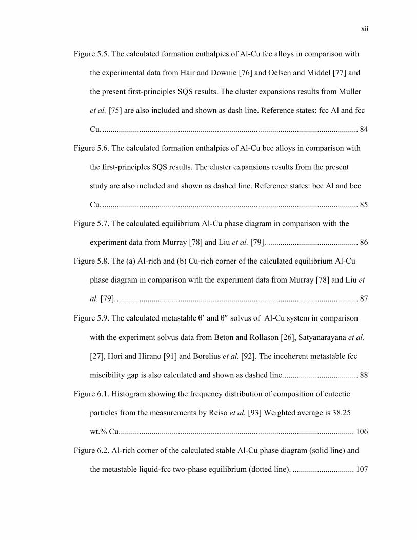
Figure 5.5. The calculated formation enthalpies of Al-Cu fcc alloys in comparison with
the experimental data from Hair and Downie [76] and Oelsen and Middel [77] and
the present first-principles SQS results. The cluster expansions results from Muller
et al. [75] are also included and shown as dash line. Reference states: fcc Al and fcc
Cu. ............................................................................................................................. 84
Figure 5.6. The calculated formation enthalpies of Al-Cu bcc alloys in comparison with
the first-principles SQS results. The cluster expansions results from the present
study are also included and shown as dashed line. Reference states: bcc Al and bcc
Cu. ............................................................................................................................. 85
Figure 5.7. The calculated equilibrium Al-Cu phase diagram in comparison with the
experiment data from Murray [78] and Liu et al. [79]. ............................................ 86
Figure 5.8. The (a) Al-rich and (b) Cu-rich corner of the calculated equilibrium Al-Cu
phase diagram in comparison with the experiment data from Murray [78] and Liu et
al. [79]....................................................................................................................... 87
Figure 5.9. The calculated metastable θ′ and θ″ solvus of Al-Cu system in comparison
with the experiment solvus data from Beton and Rollason [26], Satyanarayana et al.
[27], Hori and Hirano [91] and Borelius et al. [92]. The incoherent metastable fcc
miscibility gap is also calculated and shown as dashed line..................................... 88
Figure 6.1. Histogram showing the frequency distribution of composition of eutectic
particles from the measurements by Reiso et al. [93] Weighted average is 38.25
wt.% Cu................................................................................................................... 106
Figure 6.2. Al-rich corner of the calculated stable Al-Cu phase diagram (solid line) and
the metastable liquid-fcc two-phase equilibrium (dotted line). .............................. 107
xiii
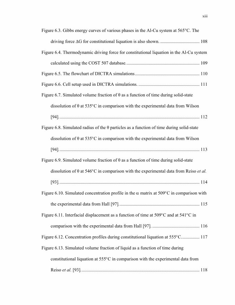
Figure 6.3. Gibbs energy curves of various phases in the Al-Cu system at 565°C. The
driving force ∆G for constitutional liquation is also shown. .................................. 108
Figure 6.4. Thermodynamic driving force for constitutional liquation in the Al-Cu system
calculated using the COST 507 database................................................................ 109
Figure 6.5. The flowchart of DICTRA simulations........................................................ 110
Figure 6.6. Cell setup used in DICTRA simulations. ..................................................... 111
Figure 6.7. Simulated volume fraction of θ as a function of time during solid-state
dissolution of θ at 535°C in comparison with the experimental data from Wilson
[94]. ......................................................................................................................... 112
Figure 6.8. Simulated radius of the θ particles as a function of time during solid-state
dissolution of θ at 535°C in comparison with the experimental data from Wilson
[94]. ......................................................................................................................... 113
Figure 6.9. Simulated volume fraction of θ as a function of time during solid-state
dissolution of θ at 546°C in comparison with the experimental data from Reiso et al.
[93]. ......................................................................................................................... 114
Figure 6.10. Simulated concentration profile in the α matrix at 509°C in comparison with
the experimental data from Hall [97]...................................................................... 115
Figure 6.11. Interfacial displacement as a function of time at 509°C and at 541°C in
comparison with the experimental data from Hall [97]. ......................................... 116
Figure 6.12. Concentration profiles during constitutional liquation at 555°C................ 117
Figure 6.13. Simulated volume fraction of liquid as a function of time during
constitutional liquation at 555°C in comparison with the experimental data from
Reiso et al. [93]....................................................................................................... 118
xiv
Figure 6.14. Simulated volume fraction of liquid as a function of time during
constitutional liquation at 565°C in comparison with the experimental data from
Wilson [94]. ............................................................................................................ 119
Figure 6.15. Simulated volume fraction of liquid as a function of time during
constitutional liquation at 585°C in comparison with the experimental data from
Wilson [94]. ............................................................................................................ 120
Figure 6.16. Solidification microstructure of liquid droplets. ........................................ 121
Figure 6.17. Scheil and DICTRA simulation of solidification of liquid from 555°C
without formation of the θ phase. ........................................................................... 122
Figure 6.18. DICTRA simulation of solidification of liquid from 555°C without
formation of the θ phase. Cooling Rate equals to 1°C/sec...................................... 123
Figure 6.19. Simulated volume fraction of liquid as a function of time during
constitutional liquation at 555°C with corrected experimental data in comparison
with the experimental data from Reiso et al. [93]. ................................................. 124
Figure 6.20. Scheil simulations of solidification of liquid from 565°C and 585°C,
respectively, without formation of the θ phase. ...................................................... 125
Figure 6.21. Calculated fraction of liquid transformed into θ with respect to undercooling.
................................................................................................................................. 126
Figure 6.22. Simulated volume fraction of liquid as a function of time during
constitutional liquation at 565°C with corrected experimental data in comparison
with the experimental data from Wilson [94]. ........................................................ 127
xv
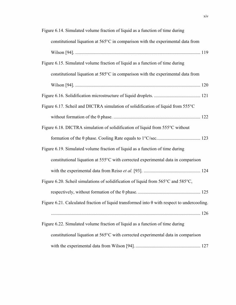
Figure 6.23. Simulated volume fraction of liquid as a function of time during
constitutional liquation at 585°C with corrected experimental data in comparison
with the experimental data from Wilson [94]. ........................................................ 128
Figure 6.24. Simulated results showing the susceptibility of a series of Al-Cu alloys to
constitutional liquation as a function of heating rate and particle size. .................. 129
Figure 7.1. Crystal structure of SQS’s in their ideal, unrelaxed forms. Gray, white and
dark spheres represent A, B and C atoms, respectively. ......................................... 146
Figure 7.2. Comparison between first-principles calculated and experimentally observed
equilibrium lattice parameters of B2 NiAl. Experimental data come from Bradley
and Taylor [8]. ........................................................................................................ 147
Figure 7.3. Comparison between first-principles calculated and experimentally observed
equilibrium volume per atom of B2 NiAl. Experimental data come from Bradley and
Taylor [8]. ............................................................................................................... 148
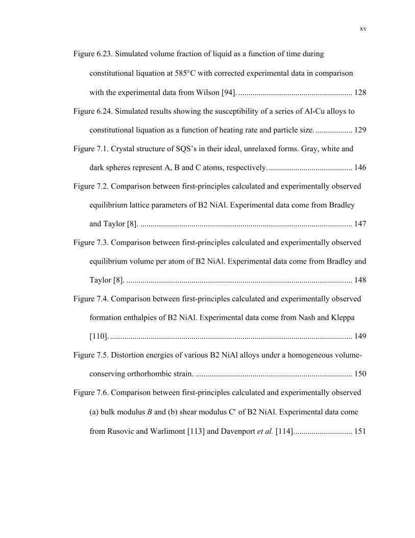
Figure 7.4. Comparison between first-principles calculated and experimentally observed
formation enthalpies of B2 NiAl. Experimental data come from Nash and Kleppa
[110]. ....................................................................................................................... 149
Figure 7.5. Distortion energies of various B2 NiAl alloys under a homogeneous volume-
conserving orthorhombic strain. ............................................................................. 150
Figure 7.6. Comparison between first-principles calculated and experimentally observed
(a) bulk modulus B and (b) shear modulus C′ of B2 NiAl. Experimental data come
from Rusovic and Warlimont [113] and Davenport et al. [114]............................. 151

xvi
LIST OF TABLES
Table 3.1. Structural descriptions of the SQS-N structures. Lattice vectors and atomic
positions are given in Cartesian coordinates, in units of a, the bcc lattice parameter.
Atomic positions are given for the ideal, unrelaxed bcc sites................................... 45
Table 3.2. Vertices of the multisite figures, given in units of a, the bcc lattice parameter.
................................................................................................................................... 46
Table 3.3. Pair and multisite correlation functions of SQS-N structures. The number in
the square brackets next to mk ,Π gives the degeneracy factor of the corresponding
figure. ........................................................................................................................ 46
Table 3.4. First principles (VASP-GGA) calculated equilibrium lattice parameter for pure
elements in the bcc structure. Spin-polarized calculations were performed for Cr and
Fe in their ferromagnetic (FM) state. ........................................................................ 46
Table 4.1. First-Principles calculated formation enthalpies (in kJ/mol) of phases in Al-Cu
system. The reference states are: fcc Al and fcc Cu. ................................................ 64
Table 5.1. Assessed thermodynamic parameters of the Al-Cu system (in SI units)......... 78
Table 5.2. Comparisons between optimized parameters with first-principles calculated
results. For the formation enthalpies, only GGA results are shown. ........................ 79
Table 6.1. Experimental conditions. ............................................................................... 104
Table 6.2. Experimental measurements of liquid undercooling. .................................... 104
Table 6.3 Kinetic parameters of the Al-Cu system. Activation energies are in J/mol and
frequency factors are in m2/s, T is in K................................................................... 104
Table 6.4. Initial conditions for DICTRA simulations. .................................................. 105

xvii
Table 6.5. Values used to calculate the volume fraction of liquid transformed into θ. .. 105
Table 7.1. Structural descriptions of the SQS-N structures. Lattice vectors and atomic
positions are given in Cartesian coordinates, in units of a, the B2 lattice parameter.
Atomic positions are given for the ideal, unrelaxed B2 sites. ................................ 143
Table 7.2. Vertices of the multisite figures, given in units of a, the B2 lattice parameter.
................................................................................................................................. 144
Table 7.3. Pair and multisite correlation functions of SQS-N structures. The number in
the square brackets next to mk ,Π gives the degeneracy factor of the corresponding
figure. ...................................................................................................................... 144
Table 7.4. Formation enthalpies (eV/defect) of isolated point defects and complex
composition-conserving defects in stoichiometric B2 NiAl. Reference states: fcc Al
and fcc Ni. ............................................................................................................... 145
Table 7.5. Effects of SQS supercell size on formation enthalpies (kJ/mol). .................. 145

xviii
ACKNOWLEDGEMENTS
First of all, I wish to express my sincere gratitude to my advisor, Dr. Zi-Kui Liu, for his
close guidance during my five-year Ph.D. study at Penn State. I also wish to thank Dr.
Long-Qing Chen, Dr. Jorge O. Sofo and Dr. Robert C. Voigt for their help and
encouragement, and serving in my thesis committee.
Special thanks need to be given to Dr. Chris Wolverton of Ford Research Laboratory for
his many help to me during my Ph.D. research.
I would also take the opportunity to thank all members of the Phases Research Lab, as
well as the faculty and staff of the Materials Science and Engineering department, for
their help to me during the my stay at Penn State.
Finally, I would like to thank my family, my wife and my parents, for their constant
encouragement and invaluable support without which this thesis could not have come
true.
1
Chapter 1. INTRODUCTION
1.1. Background
1.1.1. Heat-Treatable Aluminum Alloys
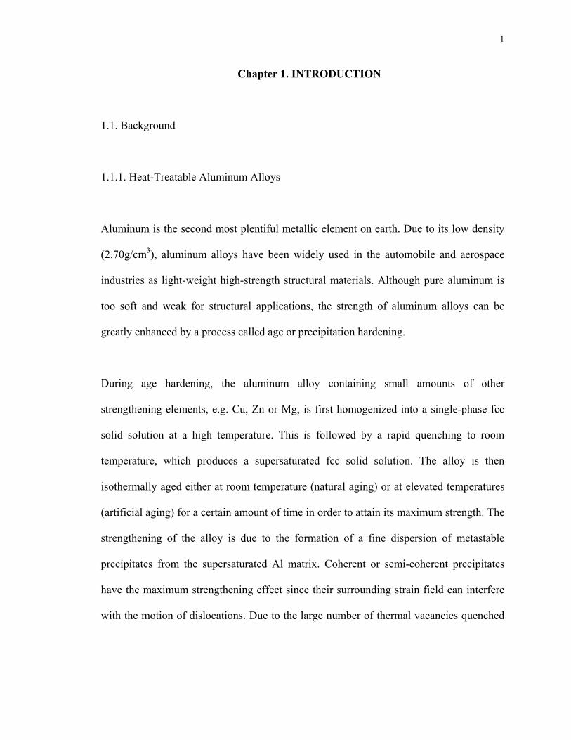
Aluminum is the second most plentiful metallic element on earth. Due to its low density
(2.70g/cm3), aluminum alloys have been widely used in the automobile and aerospace
industries as light-weight high-strength structural materials. Although pure aluminum is
too soft and weak for structural applications, the strength of aluminum alloys can be
greatly enhanced by a process called age or precipitation hardening.
During age hardening, the aluminum alloy containing small amounts of other
strengthening elements, e.g. Cu, Zn or Mg, is first homogenized into a single-phase fcc
solid solution at a high temperature. This is followed by a rapid quenching to room
temperature, which produces a supersaturated fcc solid solution. The alloy is then
isothermally aged either at room temperature (natural aging) or at elevated temperatures
(artificial aging) for a certain amount of time in order to attain its maximum strength. The
strengthening of the alloy is due to the formation of a fine dispersion of metastable
precipitates from the supersaturated Al matrix. Coherent or semi-coherent precipitates
have the maximum strengthening effect since their surrounding strain field can interfere
with the motion of dislocations. Due to the large number of thermal vacancies quenched

2
from high temperatures, the age hardening process is greatly accelerated and can occur at
low temperatures.
Al-Cu has a pivotal role as the prototype age hardening system in the development of
heat-treatable aluminum alloys. Historically, age hardening was first accidentally
discovered in the Al-Cu system. However, the reason was not elucidated until in 1938
Guinier [1] and Preston [2] independently discovered the existence of Guinier-Preston
(GP) zones. There are actually two types of GP zones, namely GP-I and GP-II. As
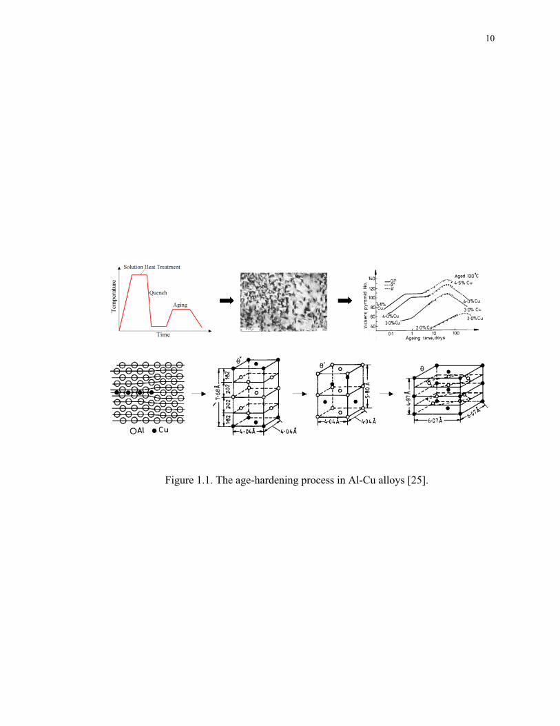
illustrated in Figure 1.1, during the age hardening of Al-Cu alloys, the precipitation
process usually starts with the formation of GP-I zones, a monolayer of pure Cu atoms on
the }100{ plane of the Al matrix. The GP-I zones are fully coherent with the Al matrix
and therefore have the lowest nucleation barrier. With longer aging time, the GP-I zones
will gradually transform into its more thermodynamically stable form, namely GP-II
zones, or θ″ (Al3Cu). θ″ is actually two layers of Cu atoms separated by three layers of Al
atoms (Cu/Al/Al/Al/Cu) and is also fully coherent with the Al matrix. Wolverton [3]
recently found that GP-I and GP-II zones are not thermodynamically distinct phases, but
rather the GP-I to GP-II transition is merely due to a size-effect: the critical size for GP-I
zones is about 150Å, beyond which they will change into GP-II zones. With even longer
aging time, θ″ will then evolve into semi-coherent θ′ (Al2Cu) and eventually the
equilibrium non-coherent θ (Al2Cu).
During the welding of many commercial heat-treatable aluminum alloys, the
strengthening precipitates such as θ′ may however lead to severe heat-affected zone

3
(HAZ) damage, which makes HAZ the weakest link in the weldment. One possible
reason for such loss of strength is due to the dissolution or coarsening of the
strengthening precipitates in the HAZ. However, much more severely, due to the rapid
heating and cooling rate experienced during normal welding operations, liquid may form
in the HAZ due to the local melting of those precipitates. This process is called
constitutional liquation as proposed by Pepe and Savage [4]. The liquid formed by
constitutional liquation may spread along the grain boundaries through the intersection of
grain boundaries with the liquated regions in the matrix. This may lead to intergranular
HAZ hot cracking during welding due to the inability of the intergranular liquid films to
sustain thermal stresses within the weldment. The solidified liquid may also embrittle the
grain boundaries and lead to intergranular fracture and cold cracking during service.
Interestingly, the absence of strengthening precipitates in the non-heat-treatable
aluminum alloys, which prevents them from achieving the same high strength as the heat-
treatable aluminum alloys, turns out to be an advantageous factor when considering
weldability. The HAZ damage incurred during welding of non-heat-treatable aluminum
alloys is much less severe and reasonable joint strengths can be obtained in the as-welded
condition without the need for post-weld heat treatment.
1.1.2. B2 Aluminides
Besides the heat-treatable aluminum alloys, intermetallic compounds based on transition
metal aluminides, e.g. NiAl and FeAl, have also recently attracted much attention. Those
intermetallic compounds possess excellent properties such as low density, high melting

4
temperature and good oxidation resistance, making them promising candidates for the
next-generation of high-temperature structural materials for aerospace applications [5-7].
Compared with the currently used Ni-based superalloys, NiAl has a lower density, higher
thermal conductivity and an over 200°C higher melting temperature. NiAl has an ordered
CsCl-type B2 structure consisting of two interpenetrating simple cubic sublattices. In the
perfectly ordered state at the 50/50 stoichiometric composition, the two sublattices are
entirely occupied by Al atoms and Ni atoms, respectively. Deviations from the ideal
stoichiometry are accommodated by the existences of constitutional point defects. The
point defect structure of NiAl is known to be of triple-defect type, i.e. Al-rich NiAl is
accommodated by the formation of Ni vacancies while Ni-rich NiAl is accommodated by
the formation of antisite Ni atoms [8].
The existences of point defects in B2 compounds are of great technological importance. It
is now well established that many important properties of B2 compounds, e.g.
mechanical properties and diffusion mechanisms, are largely dependent on the types and
concentrations of those point defects [9-11]. A full knowledge of those point defects is
therefore essential for the development of B2 aluminides. Unfortunately, direct
experimental determination of the concentrations of those point defects, e.g. using
positron annihilation method [6], is still difficult and the results are often quite
controversial [12]. This is partly due to the difficulty in creating an “ideal” homogeneous
sample. In view of this, it is highly desirable to investigate them using first-principles
approach.
5
1.1.3. Computational Materials Science
In the development of alloys with better properties to meet today’s increasingly
demanding applications, the traditional experimental trial-and-error approach becomes
more and more insufficient. This is due to the fact that most commercial alloys are multi-
component in nature and may contain as many as 10 alloying elements. It is impractical
to explore such a high dimensional composition space by experimental means.
Fortunately, with the rapidly increasing computing power we have, it is now possible to
use computers to predict the properties of alloys without the need to do experiments.
Based on computational thermodynamics, the CALPHAD (CALculation of Phase
Diagrams) [13] approach has been very successful in modeling phase equilibria and
phase transformations in complex multi-component alloys. Commercial computer
programs like Thermo-Calc [14] and DICTRA [15] have been widely used for such
purposes and sophisticated thermodynamic and kinetic databases have also been
developed using the CALPHAD approach.
Recent advances in ab-initio or first-principles calculations based on the density
functional theory (DFT) [16] have made it possible to predict from scratch the various
thermodynamic and structural properties of alloys. Combined with the cluster expansion
technique [17, 18], alloy phase diagrams can also be calculated by performing Monte-
Carlo simulations [19, 20]. These methods are truly predictive since only the atomic
numbers and crystal structure information are needed as the inputs. Actually the word
6
“ab-initio” means “from beginning”. Nevertheless, at the present stage, there still exist
several limitations that hinder the straightforward applications of the first-principles
approach to the design of alloys:
1) Despite its importance in determining finite-temperature phase stabilities [21],
first-principles calculations of vibrational entropies, e.g. using the linear-response
theory [22], are still very computationally demanding. Even so, other
contributions to entropy may also exist, such as configurational and electronic
excitation. Calculating all of these contributions and considering the coupling
between them is an even more challenging task.
2) When treating fully ordered compounds, the capability of first-principles
calculations is only limited by the total number of atoms in one unit cell and not
by the number of constituents in the compound. However, when treating multi-
component disordered phases, e.g. solution phases and compounds showing
homogeneity ranges, due to the “combinatorial explosion”, it is not
computationally tractable in the foreseeable future to directly use first-principles
calculations to treat those phases.
3) Although the cluster expansion technique has been developed to treat the
disordered phases, it is typically only applied to binary systems with very simple
underlying lattices, e.g. fcc and bcc. It is currently not directly applicable to
describe more complicated multi-component phases.

7
4) Even though a recent comparison between first-principles calculated formation
enthalpies and those in existing COST 507 [23] thermodynamic database
demonstrates that the accuracy of first-principles calculations is within a few
kJ/mol, first-principles calculations still do not have the accuracy required to
predict phase diagrams to within a few degrees to meet the industrial’s needs.
This is due to the fact that, the energy difference between two competing phases
is actually only a tiny fraction of their total energies.
1.2. Research Objectives and Thesis Outline
In heat-treatable aluminum alloys, the thermodynamically stable phases, e.g. θ, are of no
interest for industrial applications. It is the metastable phases, e.g. θ″ and θ′, which
actually contribute to the improvement of the mechanical properties of the aluminum
alloys. However, due to its semi-empirical nature, the CALPHAD method alone can not
treat metastable phases simply due to insufficient experimental data. As the consequence,
the Gibbs energies of those metastable phases are not included in the existing
thermodynamic databases for aluminum alloys, e.g. COST 507 [23]. To study the age-
hardening process in aluminum alloys, those data are however critical. Although θ′ has
been incorporated into the existing COST 507 database in a straightforward way by
Wolverton et al. [24], doing so for θ″ is not possible as COST 507 database predicts a
metastable fcc miscibility gap thermodynamically more stable than θ″, as shown in
Figure 1.2. In the present study, a thermodynamic modeling of the Al-Cu system will be
performed using a combined CALPHAD and first-principles approach. In Chapter 4,

8
first-principles calculations are performed to provide the formation enthalpies of the
stable and metastable phases in Al-Cu system. Special Quasirandom Structures (SQS’s)
are applied to model the substitutionally random fcc and bcc alloys (SQS’s for binary bcc
alloys are developed and tested in Chapter 3). Those SQS’s are rather general and can be
applied to study other systems as well. A self-consistent thermodynamic description of
the Al-Cu system including the two metastable θ″ and θ′ phases is obtained in Chapter 5.
Due to its detrimental effect during welding of heat-treatable aluminum alloys,
constitutional liquation in the model Al-Cu system will also be studied. In Chapter 6,
using the DICTRA program coupled with realistic thermodynamic and kinetic databases,
all stages of the constitutional liquation are quantitatively simulated. The critical heating
rate to avoid constitutional liquation is obtained through computer simulations. The
computational procedures developed in the present study is rather general and can be
readily extended to predict the susceptibility of commercial multi-component aluminum
alloys to constitutional liquation during welding.
Finally, due to their technological importance, SQS’s will also be developed in the
present study to model non-stoichiometric B2 compounds containing large concentrations
of constitutional point defects. In Chapter 7, such SQS’s are developed and employed to
investigate the point defects in B2 NiAl. It is unambiguously shown that, at T=0K and
zero pressure, Ni vacancies and antisite Ni atoms are the energetically favorable point
defects in Al-rich and Ni-rich B2 NiAl, respectively. The predicted formation enthalpies,
equilibrium lattice parameters and elastic constants of non-stoichiometric B2 NiAl are in

9
good agreement with experiments. Remarkably, it is found that high defect
concentrations can lead to structural instability of B2 NiAl, which explains well the
martensitic transformation observed in this compound at high Ni concentrations. Since
the SQS’s are rather general, they can be applied to study other B2 alloys as well.
10
Figure 1.1. The age-hardening process in Al-Cu alloys [25].

11
Figure 1.2. The metastable fcc miscibility gap calculated using the COST 507 database.
The experimental solvus data from Beton and Rollason [26] and Satyanarayana et al. [27]
are also shown.

12
Chapter 2. METHODOLOGY
2.1. The CALPHAD Approach
Phase diagrams are visual representations of the equilibrium state of a system as a
function of composition, temperature and pressure. They are the “roadmap” for alloys
design. Nevertheless, experimental determinations of phase diagrams are both expensive
and time-consuming. The CALPHAD approach was introduced by Kaufman [13] to
model the complex phase equilibria in multi-component alloys. Its theoretical basis is
computational thermodynamics: given the Gibbs energies of all the competing phases in a
system, the final equilibrium state at a given composition, temperature and pressure can
be calculated by minimizing the total Gibbs energy of the system:
min== ∑ pp
pGnG (2.1)
where np is the number of moles of phase p and Gp is its Gibbs energy. By keeping the
stable phases from appearing, metastable phase equilibrium can also be calculated.
In the CALPHAD approach, different thermodynamic models are used to describe
different types of phases. The Gibbs energies of pure elements in their stable, metastable
or even unstable states, the so-called “lattice-stabilities”, are taken from the SGTE pure
element database [28]. The reference state is chosen to be the enthalpies of the pure
elements in their stable states at 298.15K, commonly referred to as Standard Element
13
Reference (SER). For stoichiometric compounds with negligible homogeneity ranges,
when experimental heat capacity data are available, it is preferable to express their Gibbs
energies directly referred to the SER as follows:
( ) ( ) Lo ++++=−−−− 2ln11 TdTTcTbaxHHxG SERB
SERA
BAm
xx (2.2)
where the coefficients c and d are related to heat capacity as L+−−= TdcCp 2 . For
compounds with no heat capacity data, assuming the Neumann-Kopp rule holds, i.e.
0=∆ pC , their Gibbs energies can be expressed as:
bTaGxGxG BAxxBA
BAm +++−= ΦΦ− ooo )1(1 (2.3)
where ΦiGo is the molar Gibbs energy of pure element i in structure Φ , a and b are the
enthalpy and entropy of formation of the compound with respect to A and B in structure
ΦA and ΦB, respectively.
For solution phases such as liquid, fcc and bcc, the substitutional solution model is
usually used. Taking a binary A-B solution phase Φ for example, its Gibbs energy is
written as:
excessidealrefm GGGG ++=Φ (2.4)

14
where ΦΦ += BBAAref GxGxG oo is the Gibbs energy of mechnical mixture of pure
elements A and B, both in structure Φ . idealG denotes the contribution from
configurational entropy of mixing. Assuming random mixing of A and B atoms on a
lattice and neglecting short-range ordering (SRO), idealG can be treated by the Bragg-
Williams approximation as:
( )BBAAidealideal xxxxRTTSG lnln +=−= (2.5)
The excess term excessG is used to characterize the deviation of real alloys from the ideal
solution behaviour, which is usually expressed as a Redlich-Kister [29] polynomial:
( )∑=
Φ −=n
k
kBABA
kBA
excess xxLxxG0
, (2.6)
where ΦBA
k L , is the kth interaction parameter between the A and B atoms and can be
temperature-dependent in the form TTcTbaL kkkBAk ln, ++=Φ . ka , kb and kc are model
parameters to be evaluated from experimental data.
To model complex phases containing multiple sublattices, the compound energy
formalism (CEF) [30] is usually used. As an example, to model the A2→B2 order-
disorder transformation in a binary A-B system, a (A,B)0.5(A,B)0.5 two-sublattice model
will be used. Its Gibbs energy per mole of formula units can be written in the same form
as Eq. (2.4):
15
excessidealrefBm GGGG ++=2 (2.7)
Now the first term refG represents the contributions from all its four end-members:
BBIIB
IBAB
IIA
IBBA
IIB
IAAA
IIA
IA
ref GyyGyyGyyGyyG ::::oooo +++= (2.8)
where Iiy and II
iy are the site fractions of element i on the first and second sublattices,
respectively. jiG :o is the Gibbs energy of the compound with the first sublattice entirely
occupied by element i and the second entirely by j, be it real or hypothetical. The second
term represents contribution from configurational entropy, treated by the the Bragg-
Williams approximation assuming random mixing inside each sublattice:
)lnln(5.0)lnln(5.0 IIB
IIB
IIA
IIA
IB
IB
IA
IA
ideal yyyyRTyyyyRTG +++= (2.9)
Finally, the third term represents the contribution due to interactions within the same
sublattice:
)()( ,:,::,:,2
BABIBBAA
IA
IIB
IIABBA
IIBABA
IIA
IB
IA
Bm LyLyyyLyLyyyG +++= (2.10)
L’s are the interaction parameters and can be both composition and temperature
dependent in the Redlich-Kister [29] form (see Eq. (2.6)).
16
As illustrated in Figure 2.1, the development of thermodynamic databases using the
CALPHAD approach is usually carried out in the following four steps:
1) Do an exhaustive search for all available experimental data, e.g. thermochemical
and phase equilibrium ones, of the system to be studied. When experimental data
are insufficient, first-principles results can be used as if they are experiments.
2) Critically assess the validity of each piece of data and assign it a certain weight
according to its experimental uncertainty and relative importance.
3) Based on the crystal structure information, choose a suitable thermodynamic
model to represent each of the phases in the system. Those models generally
include some unknown phenomenological model parameters that need to be
determined.
4) Adjust all the unknown model parameters to obtain the best possible fit between
model calculations and experimental data.
The final obtained model parameters are stored in computerized databases. Once the
Gibbs energies of all the constituent subsystems have been assessed, those data can be
extrapolated to predict phase equilibria in higher-order systems.
17
2.2. First Principles Calculations
2.2.1. Fundamentals
A solid can be thought of as a collection of interacting positively charged nuclei and
negatively charged electrons. Theoretically, an exact treatment of solids can be obtained
by solving the following many-body Schrödinger’s equation involving both the nuclei
and the electrons:
),...,,,...,(),...,,,...,(ˆ21212121 nNnN rrrRRRErrrRRRH rrrrrrrrrrrr
Ψ=Ψ (2.11)
where IR ’s are the nuclei coordinates, ir ’s are the electron coordinates, H is the
Hamiltonian operator, E is the total energy of the system, N is the total number of nuclei
and n is the total number of electrons in the system. However, although theoretically
exact, it is extremely difficult to solve Eq. (2.11) due to its many-body nature. In fact, the
only system that can be solved analytically is the single-electron hydrogen atom. In
general, the Schrödinger’s equation has to be solved numerically. In the following,
several levels of approximations will be introduced.
2.2.1.1. Born-Oppenheimer Approximation
Since the nuclei are much heavier than the electrons, it can be assumed that the electrons
are always in instantaneous ground state with the nuclei. In other words, we can fix the
18
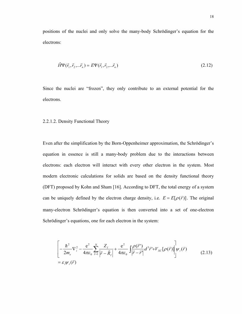
positions of the nuclei and only solve the many-body Schrödinger’s equation for the
electrons:
),...,(),...,(ˆ2121 nn rrrErrrH rrrrrr
Ψ=Ψ (2.12)
Since the nuclei are “frozen”, they only contribute to an external potential for the
electrons.
2.2.1.2. Density Functional Theory
Even after the simplification by the Born-Oppenheimer approximation, the Schrödinger’s
equation in essence is still a many-body problem due to the interactions between
electrons: each electron will interact with every other electron in the system. Most
modern electronic calculations for solids are based on the density functional theory
(DFT) proposed by Kohn and Sham [16]. According to DFT, the total energy of a system
can be uniquely defined by the electron charge density, i.e. )]([ rEE rρ= . The original
many-electron Schrödinger’s equation is then converted into a set of one-electron
Schrödinger’s equations, one for each electron in the system:
)(
)()](['')'(
4e
4e
23
0
2
10
22
2
r
rrVrdrr
rRr
Zm
ii
iXC
N
I I
Ii
e
r
rrrrr
r
rrh
ψε
ψρρπεπε
=
+
−+
−−∇− ∫∑
= (2.13)

19
The exchange correlation potential )]([ rVXCrρ is given by the functional derivative:
)]([)(
)]([ rEr
rV XCXCr
rr ρ
δρδρ = (2.14)
Nevertheless, the exact form of the exchange correlation energy )]([ rEXCrρ is unknown.
The most widely used approximation is the so-called Local Density Approximation
(LDA), which assumes that the exchange correlation energy )]([ rEXCrρ is only a function
of the local charge density in the form:
rdrrrE XCXCrrrr 3)]([)()]([ ρερρ ∫= (2.15)
where )]([ rXCrρε is the exchange-correlation energy of homogeneous electron gas of the
same charge density. LDA is expected to work well for systems with a slowly varying
charge density, but surprisingly, LDA works quite well for realistic systems as well.
One significant limitation of LDA is its overbinding of solids: lattice parameters are
usually underpredicted while cohesive energies are usually overpredicted. In an effort to
rectify the inaccuracies of LDA, the Generalized Gradient Approximation (GGA) was
introduced. GGA is a natural improvement on LDA by considering not only the local
charge density, but also its gradient. The lattice parameters calculated by GGA generally
agree noticeably better with experiments than LDA. It is worth noting here that, there is
only one LDA exchange correlation functional, i.e. the one by Ceperley and Alder [31,

20
32]. Nevertheless, there exist many versions of GGA due to the freedom in how to
incorporate the gradient term in the exchange correlation energy.
The actual first-principles total energy calculations are performed in a self-consistent
cycle. We first “guess” the initial charge density function. By solving Eq. (2.13), a new
charge density is obtained. This loop is repeated until the new charge density (or the new
total energy) does not differ much from the old one, i.e. the iteration has converged. In
practice, the nuclei also need to be relaxed into their equilibrium positions such that the
quantum-mechanical forces acting on each of them vanish. Such structural relaxations are
usually performed using a conjugate-gradient or a quasi-newton scheme. The final
obtained total energies can be used to extract the formation enthalpies of stable,
metastable or even unstable structures at T=0K using the following equation:
)()()1()()( 11 BxEAExBAEBAH xxxx −−−=∆ −− (2.16)
where E’s are the first-principles calculated total energies of structure A1-xBx and pure
elements A and B, each fully relaxed to their equilibrium (zero-pressure) geometries,
respectively.
2.2.2. Treating Disordered Alloys
Since first-principles DFT calculations rely on the construction of cells with periodic
boundary conditions, the calculations are fairly straightforward for perfectly-ordered
21
stoichiometric compounds. However, the situation is more complicated when treating
disordered alloys.
2.2.2.1. Cluster Expansions
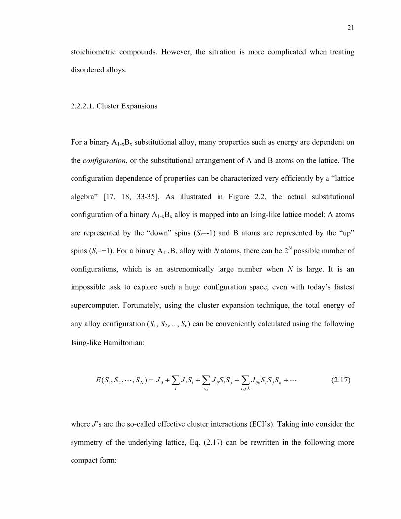
For a binary A1-xBx substitutional alloy, many properties such as energy are dependent on
the configuration, or the substitutional arrangement of A and B atoms on the lattice. The
configuration dependence of properties can be characterized very efficiently by a “lattice
algebra” [17, 18, 33-35]. As illustrated in Figure 2.2, the actual substitutional
configuration of a binary A1-xBx alloy is mapped into an Ising-like lattice model: A atoms
are represented by the “down” spins (Si=-1) and B atoms are represented by the “up”
spins (Si=+1). For a binary A1-xBx alloy with N atoms, there can be 2N possible number of
configurations, which is an astronomically large number when N is large. It is an
impossible task to explore such a huge configuration space, even with today’s fastest
supercomputer. Fortunately, using the cluster expansion technique, the total energy of
any alloy configuration (S1, S2,…, Sn) can be conveniently calculated using the following
Ising-like Hamiltonian:
LL ++++= ∑∑∑ kkji
jiijkji
jiiji
iiN SSSJSSJSJJSSSE,,,
021 ),,,( (2.17)
where J’s are the so-called effective cluster interactions (ECI’s). Taking into consider the
symmetry of the underlying lattice, Eq. (2.17) can be rewritten in the following more
compact form:

22
∑∑ ∏ Π==∈ f
ffff fi
iffN JDSJDSSSE ),,,( 21 L (2.18)
where figures f are symmetry-related groupings of lattice sites, e.g., single site, nearest-
neighbor pair, three-body figures, etc. These figures, f=(k, m) can have k vertices and
span a maximum distance of m (m=1, 2, 3… are the first, second and third-nearest
neighbors, etc.). Df denotes the degeneracy factor of figure f. fΠ is the so-called
correlation function defined as the product of the spin variable over all sites of a figure,
averaging over all symmetry-equivalent figures of the lattice. The expansion in Eq. (2.18)
is exact as long as all the figures are included. However, since the interactions between
widely separated atoms are expected to be weaker than the interactions between nearer
atoms, the expansion in Eq. (2.18) is usually truncated at certain distance to include only
a few short-ranged pair and multisite clusters.
In practice, as illustrated in Figure 2.3, the total energies of a few (30~50) pre-selected
ordered structures based on a common underlying parent lattice are first calculated by
some first-principles code like VASP. Those total energies are then used to fit all the
unknown pair and multi-body ECI’s. Subjecting the cluster expansions to Monte-Carlo
simulations, thermodynamic properties, e.g. formation enthalpies, of the alloys over the
whole composition range can be efficiently obtained.

23
2.2.2.2. Mead-Field Approach
The coherent potential approximation [36] (CPA) treats random A1-xBx alloys by
considering the average occupations of lattice sites by A and B atoms. Since it is a mean-
field approach, dependence of properties on the local environments surrounding atoms is
not treated explicitly in CPA. However, in a real (non-mean-field) random alloy, there
exists a distribution of local environments (e.g., A or B surrounded by the various AmB8-m
coordination shells with m between 0 and 8 in bcc alloys), resulting in local
environmentally-dependent quantities such as charge transfer and local displacements of
atoms from their ideal lattice positions [34, 35, 37-39]. Experimental observations [40]
also show that, even in random A1-xBx solid solutions, the average A-A, A-B and B-B
bond lengths are generally different. In size-mismatched semiconductor alloys, such local
atomic relaxations have been shown to significantly affect their thermodynamic and
electronic properties [34, 35, 37, 38].
2.2.2.3. Special Quasirandom Structures (SQS’s)
The third way to treat random A1-xBx solid solutions would be to directly construct a
large supercell and randomly decorate the host lattice with A and B atoms. Such an
approach would necessarily require very large supercells to adequately mimic the
statistics of the random alloys. Since density functional methods are computationally
constrained by the number of atoms that one can treat, this brute-force approach could be
computationally prohibitive. The concept of special quasirandom structures (SQS’s) was

24
proposed by Zunger et al. [34, 35, 41] to overcome the limitations of mean-field theories,
but without the prohibitive computational cost associated with directly constructing large
supercells with random occupancy of atoms. SQS’s are specially designed small-unit-cell
periodic structures with only a few (2~32) atoms per unit cell, which closely mimic the
most relevant, near-neighbor pair and multisite correlation functions of the random
substitutional alloys. Since the SQS approach is not a mean-field one, a distribution of
distinct local environments is maintained, the average of which corresponds to the
random alloy. Thus, a single DFT calculation of an SQS can give many important alloy
properties [34, 35, 41] (e.g. equilibrium bond lengths, charge transfer, formation
enthalpies, etc.) which depend on the existence of those distinct local environments.
Furthermore, since the SQS approach is geared towards relatively small-unit-cells,
essentially any DFT method can be applied to this approach, including full-potential
methods capable of accurately capturing the effects of atomic relaxation.
The advantage of the SQS approach is that, in order to obtain a fully converged cluster
expansion for a given alloy, the energies of about 30~50 ordered structures have to be
obtained in their fully relaxed geometries, which is still a quite laborious task. In contrast,
using SQS’s, only one single calculation is required to obtain the various properties of a
random alloy. The SQS approach has been used extensively to study the formation
enthalpies, bond length distributions, density of states, band gaps and optical properties in
semiconductor alloys [34, 35, 41]. They have also been applied to investigate the local
lattice relaxations in size-mismatched transition metal alloys [37-39, 42] and to predict
the formation enthalpies of Al-based fcc alloys [43]. However, to date, all the
25
applications of the SQS methodology are for systems in which the substitutional alloy
problem is fcc-based (e.g., fcc-based metals, zinc-blende-based semiconductors, or rock-
salt-based oxides). No SQS’s for the bcc structure exist in the literature. Therefore, in
Chapter 3, SQS’s will be developed for binary bcc alloys at compositions x=0.25, 0.50
and 0.75, respectively. Since these SQS’s are quite general, they can be applied to any
binary bcc alloy.

26
Figure 2.1. Thermodynamic database development using CALPHAD.

27
(a) Alloy configuration
(b) Lattice model
Figure 2.2. Mapping substitutional A1-xBx alloy into a Ising-like lattice model.

28
Figure 2.3. The flowchart of Alloy-Theoretic Automated Toolkit (ATAT) [20, 44].

29
Chapter 3. SPECIAL QUASIRANDOM STRUCTURES FOR BINARY BCC
ALLOYS
3.1. Theoretical Basis of SQS’s
For the perfectly random A1-xBx bcc alloys, there is no correlation in the occupation
between various sites, and therefore correlation function mk ,Π simply becomes the
product of the lattice-averaged site variable, which is related to the composition by < Si >
= 2x−1. Thus, for the perfectly random alloy, the pair and multisite correlation functions
mk ,Π are given quite simply as:
( )kRmk x 12, −=Π (3.1)
The SQS approach amounts to finding small-unit-cell ordered structures that possess
( )RmkSQSmk ,, Π≅Π for as many figures as possible. Admittedly, describing random
alloys by small unit-cell periodically-repeated structures will surely introduce erroneous
correlations beyond a certain distance. However, as already mentioned, since interactions
between nearest neighbors are generally more important than interactions between more
distant neighbors, the SQS’s can be constructed in such as way that they exactly
reproduce the correlation functions of a random alloy between the first few nearest
neighbors, deferring errors due to periodicity to more distant neighbors.

30
3.2. Generation of the SQS’s
In the present study, various SQS-N structures (with N=2, 4, 8 and 16 atoms per unit cell)
are generated for the random bcc alloys at composition x=0.50 and 0.75 using the gensqs
code in ATAT [20, 44]. For each composition x, the procedure can be described as
follows:
1) Using gensqs, exhaustively generate all structures based on the bcc lattice with N
atoms per unit cell and composition x.
2) Construct the pair and multisite correlation functions mk ,Π for each structure.
3) Finally, search for the structure(s) that best match the correlation functions of
random alloys over a specified set of pair and multisite figures.
The SQS-16 structure for x=0.5 is obtained by requiring that its pair correlation functions
be identical to those of the random alloy up to the fifth-nearest neighbor. Nevertheless,
for x=0.75, no SQS-16 structures satisfy this criterion. Therefore, we instead choose a
structure whose pair correlation functions are identical to the random alloy up to the
fourth-nearest neighbor. The other SQS-N structures with N=2, 4 and 8 atoms per unit
cell are generated using an analogous approach. Of course, in general, the smaller the unit
cell, the fewer pair correlations that match those of the random alloy.
31
The lattice vectors and atomic positions of the obtained SQS-N structures in their ideal,
unrelaxed forms are given in Table 3.1, all in Cartesian coordinates. The definitions of
the multisite figures considered here are given in Table 3.2. In Table 3.3, the pair and
multisite correlation functions of the SQS-N structures presented in Table 3.1 are
compared with those of the corresponding random alloys. We also give an estimate of the
errors due to periodicity, estimated as ∑=
−−Π4
1
22,2 ))12((
mm x , over the first four neighbor
pairs. These errors are also shown in Table 3.3, and they rapidly decrease with increasing
N. We note that the SQS-N structures for x=0.25 are obtained simply by switching the A
and B atoms in SQS-N for x=0.75. Since this amounts to replacing all of the spin
variables by Si → -Si, all even-body correlations are equivalent for x=0.25 and x=0.75,
while all odd-body correlations simply change sign. Thus, the three-body figures are
largely responsible for asymmetries in the formation energies between x=0.25 and
x=0.75.
In all calculations in the present study, unless specifically noted, we use the 16-atom
SQS’s to represent the random bcc alloys. The extent to which they match the random
alloy correlations is comparable to those of the existing 16-atom SQS’s for the fcc
structure (see Appendix A), which reproduce the pair correlation functions of perfectly
random fcc alloys accurately up to the seventh-nearest neighbor at x=0.5 and third-
nearest neighbor at x=0.75 [43]. SQS-16 for x=0.5 is a triclinic-type structure with space
group 1P (space group No. 2 in the International Tables of Crystallography), and SQS-
16 for x=0.75 is a monoclinic-type structure with space group Cm (space group No. 8 in
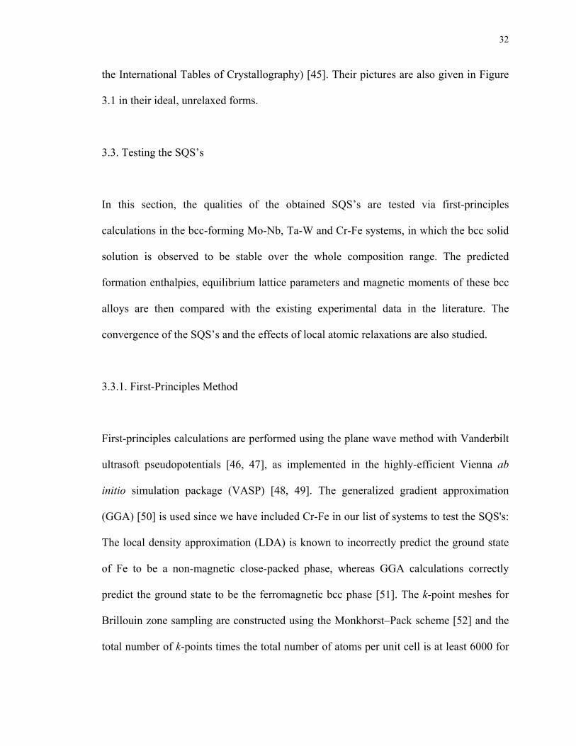
32
the International Tables of Crystallography) [45]. Their pictures are also given in Figure
3.1 in their ideal, unrelaxed forms.
3.3. Testing the SQS’s
In this section, the qualities of the obtained SQS’s are tested via first-principles
calculations in the bcc-forming Mo-Nb, Ta-W and Cr-Fe systems, in which the bcc solid
solution is observed to be stable over the whole composition range. The predicted
formation enthalpies, equilibrium lattice parameters and magnetic moments of these bcc
alloys are then compared with the existing experimental data in the literature. The
convergence of the SQS’s and the effects of local atomic relaxations are also studied.
3.3.1. First-Principles Method
First-principles calculations are performed using the plane wave method with Vanderbilt
ultrasoft pseudopotentials [46, 47], as implemented in the highly-efficient Vienna ab
initio simulation package (VASP) [48, 49]. The generalized gradient approximation
(GGA) [50] is used since we have included Cr-Fe in our list of systems to test the SQS's:
The local density approximation (LDA) is known to incorrectly predict the ground state
of Fe to be a non-magnetic close-packed phase, whereas GGA calculations correctly
predict the ground state to be the ferromagnetic bcc phase [51]. The k-point meshes for
Brillouin zone sampling are constructed using the Monkhorst–Pack scheme [52] and the
total number of k-points times the total number of atoms per unit cell is at least 6000 for

33
all systems. A plane wave cutoff energy Ecut of 233.1, 235.2 and 296.9 eV are used for
Mo-Nb, Ta-W and Cr-Fe system, respectively. All calculations include scalar relativistic
corrections (i.e., no spin-orbit interaction).
Spin-polarized calculations are performed for the Cr-Fe alloys, whereas all other
calculations are nonmagnetic. Pure bcc Fe is ferromagnetic while pure bcc Cr is
antiferromagnetic with incommensurate spin density waves [53]. This leads to a quite
complicated magnetic structure in the Cr1-xFex bcc alloys at low temperatures [54], which
will not be investigated in the present study. Instead, since our SQS calculations are
performed at compositions x=0.25, 0.5 and 0.75, all larger than the critical composition
x=0.2 beyond which the Cr1-xFex bcc alloy becomes ferromagnetic [55], we assume a
ferromagnetic structure for the Cr-Fe bcc alloys in our spin-polarized calculations.
By computing the quantum-mechanical forces and stress tensor, structural and atomic
relaxations are performed and all atoms are relaxed into their equilibrium positions using
a conjugate-gradient scheme. For the bcc alloys considered in the present study, the
SQS’s are fully relaxed with respect to both the volume and shape of the unit cell as well
as all the atomic positions. In all our calculations, the magnitudes of cell vector
distortions of the fully relaxed SQS’s with respect to their ideal, unrelaxed unit cells are
very small, indicating structural stability of the bcc lattice for these systems.
The formation enthalpies of the random bcc alloys are obtained as:
34
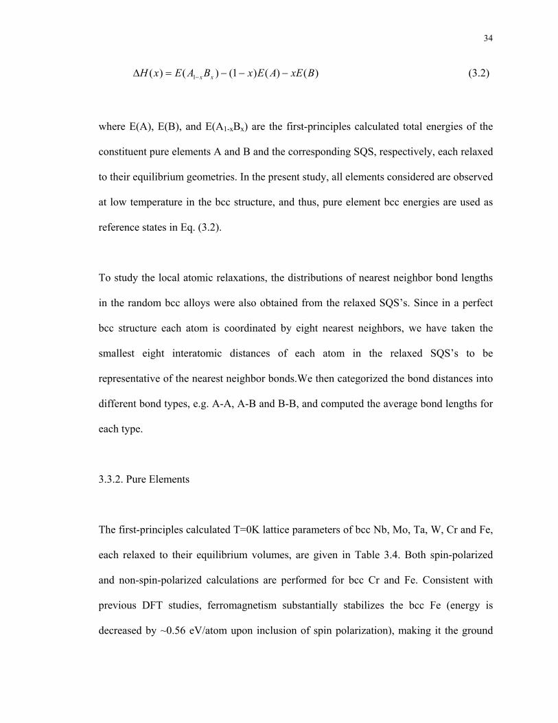
)()()1()()( 1 BxEAExBAExH xx −−−=∆ − (3.2)
where E(A), E(B), and E(A1-xBx) are the first-principles calculated total energies of the
constituent pure elements A and B and the corresponding SQS, respectively, each relaxed
to their equilibrium geometries. In the present study, all elements considered are observed
at low temperature in the bcc structure, and thus, pure element bcc energies are used as
reference states in Eq. (3.2).
To study the local atomic relaxations, the distributions of nearest neighbor bond lengths
in the random bcc alloys were also obtained from the relaxed SQS’s. Since in a perfect
bcc structure each atom is coordinated by eight nearest neighbors, we have taken the
smallest eight interatomic distances of each atom in the relaxed SQS’s to be
representative of the nearest neighbor bonds.We then categorized the bond distances into
different bond types, e.g. A-A, A-B and B-B, and computed the average bond lengths for
each type.
3.3.2. Pure Elements
The first-principles calculated T=0K lattice parameters of bcc Nb, Mo, Ta, W, Cr and Fe,
each relaxed to their equilibrium volumes, are given in Table 3.4. Both spin-polarized
and non-spin-polarized calculations are performed for bcc Cr and Fe. Consistent with
previous DFT studies, ferromagnetism substantially stabilizes the bcc Fe (energy is
decreased by ~0.56 eV/atom upon inclusion of spin polarization), making it the ground

35
state of Fe. Spin-polarized, ferromagnetic calculations for Cr resulted in a non-magnetic
solution. According to Table 3.4, the lattice mismatch (defined as aa∆ ) in the Mo-Nb,
Ta-W, and Cr-Fe alloy systems are found to be 4.3%, 3.7% and 0%, respectively.
3.3.3. Mo-Nb Bcc Alloys
Mo and Nb form a continuous bcc solid solution. No intermediate phases have been
reported in this system [56]. The equilibrium lattice parameters of Mo-Nb bcc alloys
obtained from the relaxed SQS’s are plotted in Figure 3.2 together with those of the pure
bcc Mo and Nb given in Table 3.4. The experimental measurements by Goldschmidt and
Brand [57] and Catterall and Barker [58] are also included for comparison. Our
calculations are in good agreement with experiments. Both show a small negative
deviation from the Vegard’s law, i.e.
)()()1()( 1 BxaAaxBAa xx +−=− (3.3)
where )( 1 xx BAa − , )(Aa and )(Ba are the equilibrium lattice parameter of alloy A1-xBx
and constituent pure elements A and B, respectively. In Figure 3.3, the predicted
formation enthalpies of random Mo-Nb bcc alloys are compared with the experimental
measurements by Singhal and Worrell [56] at 1200K using a solid state galvanic cell.
Fairly satisfactorily agreement has been reached with the largest discrepancy less than
2kJ/mol. Sigli et al. [59] also calculated the formation enthalpies of Mo-Nb bcc alloys
using the TB-CPA-GPM approach. For the purpose of comparison, their results are also

36
show in Figure 3.3, which agree quite well with our SQS’s results. In all three cases, the
asymmetry of the formation enthalpy with respect to x=0.50 is quite small.
The negative formation enthalpies indicate that Mo-Nb is an ordering-type system. Sigli
et al. [59] predicted that an ordered B2 structure is stable in Mo-Nb below 830K.
Neglecting the effects of vibrational entropy and assuming ideal configurational entropy
of mixing for the Mo1-xNbx bcc solid solution, i.e.:
( ))1ln()1()ln( xxxxRSideal −−+−=∆ (3.4)
We obtain a crude estimate the A2-B2 order-disorder transition temperature at
composition x=0.5 in Mo-Nb using the following equation:
2ln)5.0( 2
RHxHT B
SQSbcc
c∆−=∆
≈ (3.5)
Our first-principles calculation of the formation enthalpy of the fully ordered MoNb B2
structure gives –13.1 kJ/mol. Using Eq. (3.5), we thus obtain Tc≈731K, in good
agreement with the temperature of 830K predicted by Sigli et al. [59] Since this
temperature is relatively low compared with the melting temperature of Mo (2896K) and
Nb (2750K), sluggish kinetics might explain why the B2 structure or other ordered
phases have not been observed experimentally. However, our results do predict the
existence of ordered structures in Mo-Nb which to date, have not yet been observed.
37
Therefore, we assert that experimental re-examination of the low-temperature phase
stability of Mo-Nb would be of interest.
3.3.4. Ta-W Bcc Alloys
Ta and W also form a continuous bcc solid solution with no intermediate phases [60].
The predicted equilibrium lattice parameters of Ta-W bcc alloys are shown in Figure 3.4,
in good agreement with the existing experimental measurements [61]. Both show a
negative deviation from the Vegard’s law. In Figure 3.5, the predicted formation
enthalpies of random Ta-W bcc alloys are compared with the experimental solid state
galvanic cell measurements of Singhal and Worrell [60]. In Figure 3.4 and Figure 3.5 we
also show the formation enthalpies of random Ta-W bcc alloys calculated by Turchi et al.
[62] using the TB-LMTO-ASA-CPA approach. Interestingly, although experimental
formation enthalpies exhibit a strong asymmetry towards the Ta-rich side, both SQS and
CPA calculated formation enthalpies exhibit a strong asymmetry towards the W-rich side.
Such large discrepancies between our calculations and experimental measurements on the
W-rich side may be due to the slow kinetics at the experimental temperature of 1200K,
which makes thermodynamic equilibrium difficult to reach, as was also pointed out by
Turchi et al. [62] To ascertain this, we examined the tracer diffusivity of Ta in bcc W at
1200K using the Arrhenius relation obtained by Arkhipova et al. [63]:
)601241(102.6 4 RTExpDWTa −×= − (3.6)

38
and we obtained an extremely low value of 4.186×10⁻³⁰ m2/s. The fact that WTaD
dominates the interdiffusion coefficients in the W-rich Ta-W bcc alloys could explain
why the discrepancies between SQS calculations and experiments are largest on the W-
rich side. However, we should also note other possibilities to explain this discrepancy:
1) Our SQS are constructed to mimic the perfectly random state, and thus short-
range order in these alloys could also contribute to the discrepancy.
2) Although the SQS possess many pair and multi-body correlations that match the
random alloy statistics, there are deviations from the random alloy correlations for
longer-ranged pair and other multi-body interactions. If some of these interactions
are significant, they could contribute to the discrepancy.
3) Finally, we should note that experimental measurements of formation enthalpies
down to an accuracy of 1 kJ/mol are quite difficult, and it is possible that the
experimental data is partly responsible for the discrepancy.
It is interesting that the results of Turchi et al. [62] overestimate the formation enthalpies
relative to our SQS results even though their CPA calculations ignore such important
physical effects as atomic relaxations, which will lower the formation enthalpy. We
attribute such apparent discrepancies to the atomic sphere approximation (ASA)
employed in their CPA calculations.
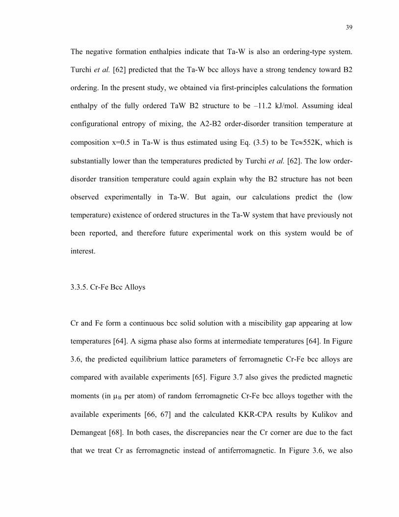
39
The negative formation enthalpies indicate that Ta-W is also an ordering-type system.
Turchi et al. [62] predicted that the Ta-W bcc alloys have a strong tendency toward B2
ordering. In the present study, we obtained via first-principles calculations the formation
enthalpy of the fully ordered TaW B2 structure to be –11.2 kJ/mol. Assuming ideal
configurational entropy of mixing, the A2-B2 order-disorder transition temperature at
composition x=0.5 in Ta-W is thus estimated using Eq. (3.5) to be Tc≈552K, which is
substantially lower than the temperatures predicted by Turchi et al. [62]. The low order-
disorder transition temperature could again explain why the B2 structure has not been
observed experimentally in Ta-W. But again, our calculations predict the (low
temperature) existence of ordered structures in the Ta-W system that have previously not
been reported, and therefore future experimental work on this system would be of
interest.
3.3.5. Cr-Fe Bcc Alloys
Cr and Fe form a continuous bcc solid solution with a miscibility gap appearing at low
temperatures [64]. A sigma phase also forms at intermediate temperatures [64]. In Figure
3.6, the predicted equilibrium lattice parameters of ferromagnetic Cr-Fe bcc alloys are
compared with available experiments [65]. Figure 3.7 also gives the predicted magnetic
moments (in µB per atom) of random ferromagnetic Cr-Fe bcc alloys together with the
available experiments [66, 67] and the calculated KKR-CPA results by Kulikov and
Demangeat [68]. In both cases, the discrepancies near the Cr corner are due to the fact
that we treat Cr as ferromagnetic instead of antiferromagnetic. In Figure 3.6, we also

40
include our calculated equilibrium lattice parameter of antiferromagnetic bcc Cr with a
commensurate wave vector using a B2 unit cell, which is in good agreement with the
measured value. We found that antiferromagnetism lowers the energy of bcc Cr by
~0.046 eV/atom.
Dench [69] experimentally measured the formation enthalpies of bcc Cr-Fe alloys at
1400K. This temperature is well above the Curie (or Néel) temperature of Cr-Fe bcc
alloys [64], therefore, the measured alloys are all in the paramagnetic state. However, the
present spin-polarized calculations correspond to the ferromagnetic state of the alloys.
Akai and Dederichs [70] and Olsson et al. [71] calculated using the KKR-CPA and FCD-
EMTO-CPA approach, respectively, the structural energy differences between the
paramagnetic and ferromagnetic states of random Cr-Fe bcc alloys, PMFME →∆ , which are
found to be substantial in the Cr-Fe system. In both studies, the disordered local moment
(DLM) model was used, which treats the paramagnetic Cr1-xFex alloy as a random
quaternary (Cr↑,Cr↓)1-x(Fe↑,Fe↓)x system with equal number of up-spin and down-spin
atoms. Since the Cr-Fe system is a perfectly lattice-matched system with aa∆ <1%, one
might expect that the atomic relaxations are small, and that the neglect of them in the
CPA should represent only a minor approximation. We will investigate more the
relaxation behavior of this alloy below.
Figure 3.8 shows the CPA calculated formation enthalpy difference between the
paramagnetic and ferromagnetic states of Cr-Fe bcc alloys [70, 71] defined as:
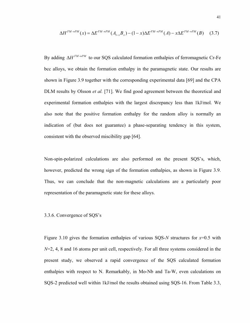
41
)()()1()()( 1 BExAExBAExH PMFMPMFMxx
PMFMPMFM →→−
→→ ∆−∆−−∆=∆ (3.7)
By adding PMFMH →∆ to our SQS calculated formation enthalpies of ferromagnetic Cr-Fe
bcc alloys, we obtain the formation enthalpy in the paramagnetic state. Our results are
shown in Figure 3.9 together with the corresponding experimental data [69] and the CPA
DLM results by Olsson et al. [71]. We find good agreement between the theoretical and
experimental formation enthalpies with the largest discrepancy less than 1kJ/mol. We
also note that the positive formation enthalpy for the random alloy is normally an
indication of (but does not guarantee) a phase-separating tendency in this system,
consistent with the observed miscibility gap [64].
Non-spin-polarized calculations are also performed on the present SQS’s, which,
however, predicted the wrong sign of the formation enthalpies, as shown in Figure 3.9.
Thus, we can conclude that the non-magnetic calculations are a particularly poor
representation of the paramagnetic state for these alloys.
3.3.6. Convergence of SQS’s
Figure 3.10 gives the formation enthalpies of various SQS-N structures for x=0.5 with
N=2, 4, 8 and 16 atoms per unit cell, respectively. For all three systems considered in the
present study, we observed a rapid convergence of the SQS calculated formation
enthalpies with respect to N. Remarkably, in Mo-Nb and Ta-W, even calculations on
SQS-2 predicted well within 1kJ/mol the results obtained using SQS-16. From Table 3.3,
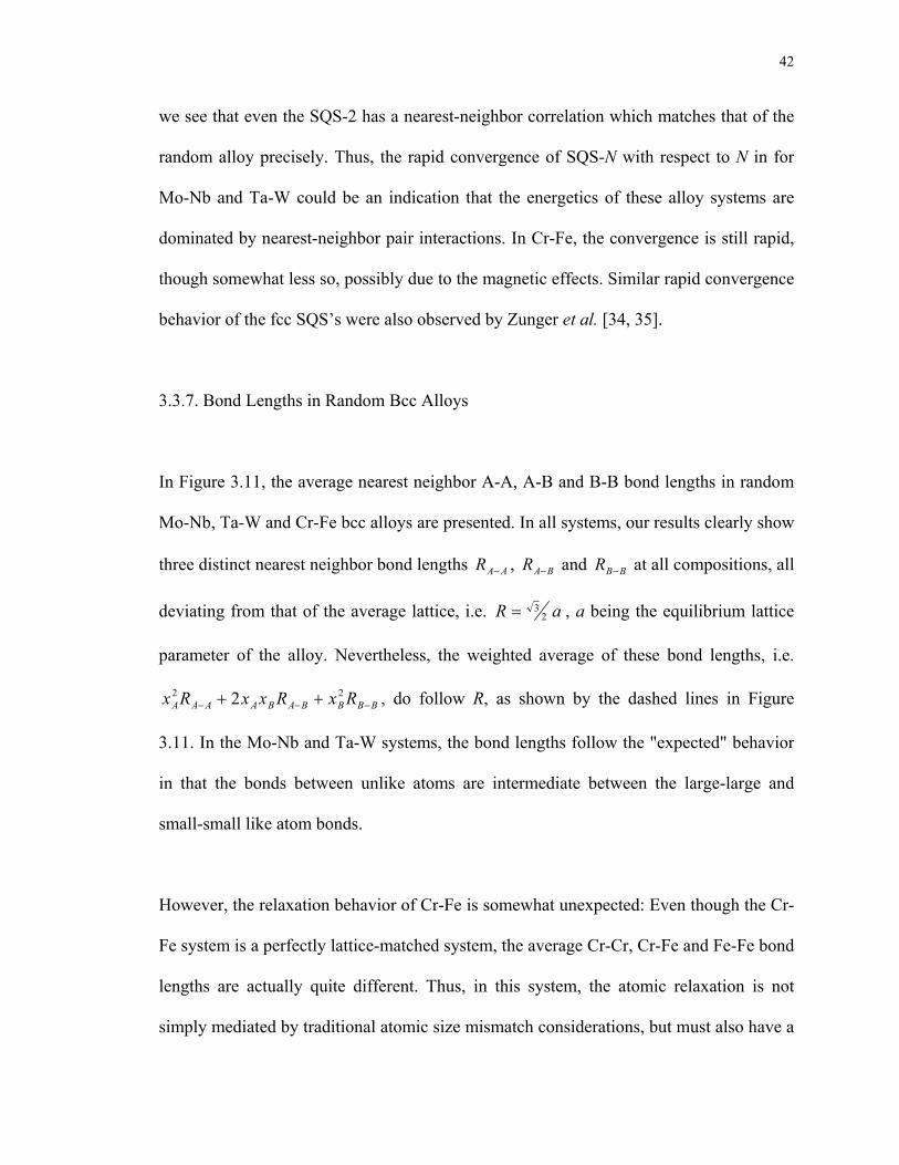
42
we see that even the SQS-2 has a nearest-neighbor correlation which matches that of the
random alloy precisely. Thus, the rapid convergence of SQS-N with respect to N in for
Mo-Nb and Ta-W could be an indication that the energetics of these alloy systems are
dominated by nearest-neighbor pair interactions. In Cr-Fe, the convergence is still rapid,
though somewhat less so, possibly due to the magnetic effects. Similar rapid convergence
behavior of the fcc SQS’s were also observed by Zunger et al. [34, 35].
3.3.7. Bond Lengths in Random Bcc Alloys
In Figure 3.11, the average nearest neighbor A-A, A-B and B-B bond lengths in random
Mo-Nb, Ta-W and Cr-Fe bcc alloys are presented. In all systems, our results clearly show
three distinct nearest neighbor bond lengths AAR − , BAR − and BBR − at all compositions, all
deviating from that of the average lattice, i.e. aR 23= , a being the equilibrium lattice
parameter of the alloy. Nevertheless, the weighted average of these bond lengths, i.e.
BBBBABAAAA RxRxxRx −−− ++ 22 2 , do follow R, as shown by the dashed lines in Figure
3.11. In the Mo-Nb and Ta-W systems, the bond lengths follow the "expected" behavior
in that the bonds between unlike atoms are intermediate between the large-large and
small-small like atom bonds.
However, the relaxation behavior of Cr-Fe is somewhat unexpected: Even though the Cr-
Fe system is a perfectly lattice-matched system, the average Cr-Cr, Cr-Fe and Fe-Fe bond
lengths are actually quite different. Thus, in this system, the atomic relaxation is not
simply mediated by traditional atomic size mismatch considerations, but must also have a
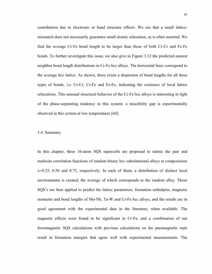
43
contribution due to electronic or band structure effects. We see that a small lattice-
mismatch does not necessarily guarantee small atomic relaxation, as is often asserted. We
find the average Cr-Fe bond length to be larger than those of both Cr-Cr and Fe-Fe
bonds. To further investigate this issue, we also give in Figure 3.12 the predicted nearest
neighbor bond length distributions in Cr-Fe bcc alloys. The horizontal lines correspond to
the average bcc lattice. As shown, there exists a dispersion of bond lengths for all three
types of bonds, i.e. Cr-Cr, Cr-Fe and Fe-Fe, indicating the existence of local lattice
relaxations. This unusual structural behavior of the Cr-Fe bcc alloys is interesting in light
of the phase-separating tendency in this system: a miscibility gap is experimentally
observed in this system at low temperatures [64].
3.4. Summary
In this chapter, three 16-atom SQS supercells are proposed to mimic the pair and
multisite correlation functions of random binary bcc substitutional alloys at compositions
x=0.25, 0.50 and 0.75, respectively. In each of them, a distribution of distinct local
environments is created, the average of which corresponds to the random alloy. Those
SQS’s are then applied to predict the lattice parameters, formation enthalpies, magnetic
moments and bond lengths of Mo-Nb, Ta-W and Cr-Fe bcc alloys, and the results are in
good agreement with the experimental data in the literature, when available. The
magnetic effects were found to be significant in Cr-Fe, and a combination of our
ferromagnetic SQS calculations with previous calculations on the paramagnetic state
result in formation energies that agree well with experimental measurements. The
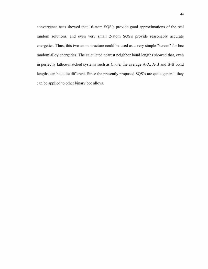
44
convergence tests showed that 16-atom SQS’s provide good approximations of the real
random solutions, and even very small 2-atom SQS's provide reasonably accurate
energetics. Thus, this two-atom structure could be used as a very simple "screen" for bcc
random alloy energetics. The calculated nearest neighbor bond lengths showed that, even
in perfectly lattice-matched systems such as Cr-Fe, the average A-A, A-B and B-B bond
lengths can be quite different. Since the presently proposed SQS’s are quite general, they
can be applied to other binary bcc alloys.
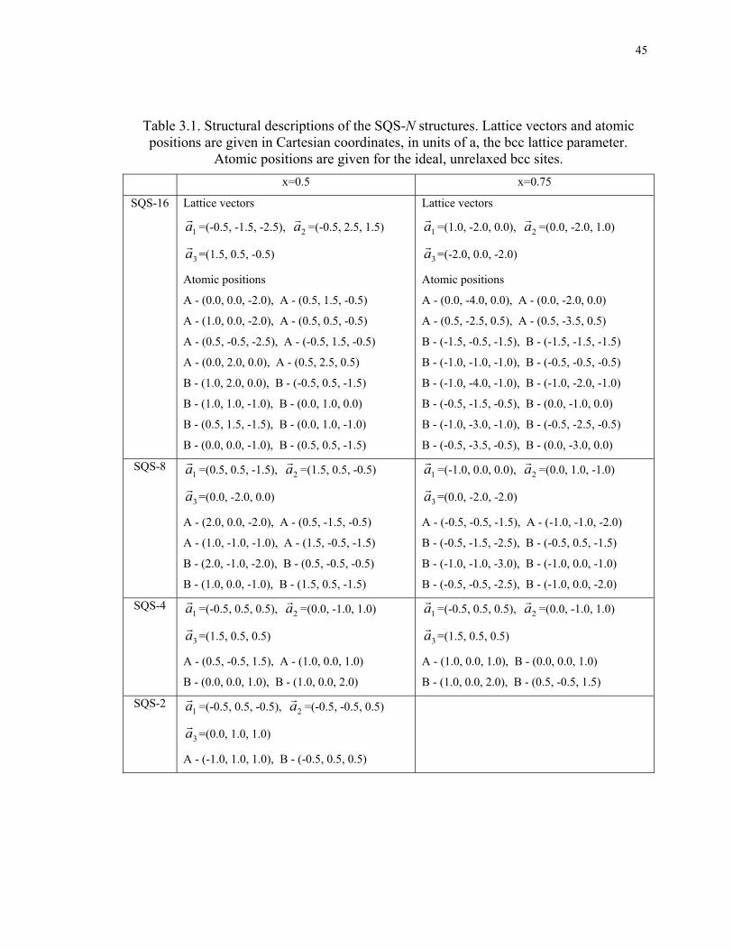
45
Table 3.1. Structural descriptions of the SQS-N structures. Lattice vectors and atomic positions are given in Cartesian coordinates, in units of a, the bcc lattice parameter.
Atomic positions are given for the ideal, unrelaxed bcc sites. x=0.5 x=0.75
SQS-16 Lattice vectors
1ar =(-0.5, -1.5, -2.5), 2ar =(-0.5, 2.5, 1.5)
3ar =(1.5, 0.5, -0.5)
Atomic positions
A - (0.0, 0.0, -2.0), A - (0.5, 1.5, -0.5)
A - (1.0, 0.0, -2.0), A - (0.5, 0.5, -0.5)
A - (0.5, -0.5, -2.5), A - (-0.5, 1.5, -0.5)
A - (0.0, 2.0, 0.0), A - (0.5, 2.5, 0.5)
B - (1.0, 2.0, 0.0), B - (-0.5, 0.5, -1.5)
B - (1.0, 1.0, -1.0), B - (0.0, 1.0, 0.0)
B - (0.5, 1.5, -1.5), B - (0.0, 1.0, -1.0)
B - (0.0, 0.0, -1.0), B - (0.5, 0.5, -1.5)
Lattice vectors
1ar =(1.0, -2.0, 0.0), 2ar =(0.0, -2.0, 1.0)
3ar =(-2.0, 0.0, -2.0)
Atomic positions
A - (0.0, -4.0, 0.0), A - (0.0, -2.0, 0.0)
A - (0.5, -2.5, 0.5), A - (0.5, -3.5, 0.5)
B - (-1.5, -0.5, -1.5), B - (-1.5, -1.5, -1.5)
B - (-1.0, -1.0, -1.0), B - (-0.5, -0.5, -0.5)
B - (-1.0, -4.0, -1.0), B - (-1.0, -2.0, -1.0)
B - (-0.5, -1.5, -0.5), B - (0.0, -1.0, 0.0)
B - (-1.0, -3.0, -1.0), B - (-0.5, -2.5, -0.5)
B - (-0.5, -3.5, -0.5), B - (0.0, -3.0, 0.0) SQS-8
1ar =(0.5, 0.5, -1.5), 2ar =(1.5, 0.5, -0.5)
3ar =(0.0, -2.0, 0.0)
A - (2.0, 0.0, -2.0), A - (0.5, -1.5, -0.5)
A - (1.0, -1.0, -1.0), A - (1.5, -0.5, -1.5)
B - (2.0, -1.0, -2.0), B - (0.5, -0.5, -0.5)
B - (1.0, 0.0, -1.0), B - (1.5, 0.5, -1.5)
1ar =(-1.0, 0.0, 0.0), 2ar =(0.0, 1.0, -1.0)
3ar =(0.0, -2.0, -2.0)
A - (-0.5, -0.5, -1.5), A - (-1.0, -1.0, -2.0)
B - (-0.5, -1.5, -2.5), B - (-0.5, 0.5, -1.5)
B - (-1.0, -1.0, -3.0), B - (-1.0, 0.0, -1.0)
B - (-0.5, -0.5, -2.5), B - (-1.0, 0.0, -2.0) SQS-4
1ar =(-0.5, 0.5, 0.5), 2ar =(0.0, -1.0, 1.0)
3ar =(1.5, 0.5, 0.5)
A - (0.5, -0.5, 1.5), A - (1.0, 0.0, 1.0)
B - (0.0, 0.0, 1.0), B - (1.0, 0.0, 2.0)
1ar =(-0.5, 0.5, 0.5), 2ar =(0.0, -1.0, 1.0)
3ar =(1.5, 0.5, 0.5)
A - (1.0, 0.0, 1.0), B - (0.0, 0.0, 1.0)
B - (1.0, 0.0, 2.0), B - (0.5, -0.5, 1.5) SQS-2
1ar =(-0.5, 0.5, -0.5), 2ar =(-0.5, -0.5, 0.5)
3ar =(0.0, 1.0, 1.0)
A - (-1.0, 1.0, 1.0), B - (-0.5, 0.5, 0.5)
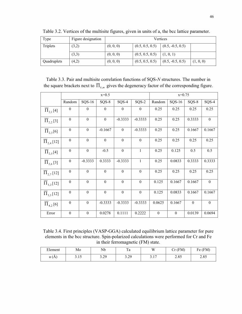
46
Table 3.2. Vertices of the multisite figures, given in units of a, the bcc lattice parameter. Type Figure designation Vertices
(3,2) (0, 0, 0) (0.5, 0.5, 0.5) (0.5, -0.5, 0.5) Triplets
(3,3) (0, 0, 0) (0.5, 0.5, 0.5) (1, 0, 1)
Quadruplets (4,2) (0, 0, 0) (0.5, 0.5, 0.5) (0.5, -0.5, 0.5) (1, 0, 0)
Table 3.3. Pair and multisite correlation functions of SQS-N structures. The number in the square brackets next to mk ,Π gives the degeneracy factor of the corresponding figure.
x=0.5 x=0.75
Random SQS-16 SQS-8 SQS-4 SQS-2 Random SQS-16 SQS-8 SQS-4
1,2Π [4] 0 0 0 0 0 0.25 0.25 0.25 0.25
2,2Π [3] 0 0 0 -0.3333 -0.3333 0.25 0.25 0.3333 0
3,2Π [6] 0 0 -0.1667 0 -0.3333 0.25 0.25 0.1667 0.1667
4,2Π [12] 0 0 0 0 0 0.25 0.25 0.25 0.25
5,2Π [4] 0 0 -0.5 0 1 0.25 0.125 0.5 0.5
6,2Π [3] 0 -0.3333 0.3333 -0.3333 1 0.25 0.0833 0.3333 0.3333
7,2Π [12] 0 0 0 0 0 0.25 0.25 0.25 0.25
2,3Π [12] 0 0 0 0 0 0.125 0.1667 0.1667 0
3,3Π [12] 0 0 0 0 0 0.125 0.0833 0.1667 0.1667
2,4Π [6] 0 0 -0.3333 -0.3333 -0.3333 0.0625 0.1667 0 0
Error 0 0 0.0278 0.1111 0.2222 0 0 0.0139 0.0694
Table 3.4. First principles (VASP-GGA) calculated equilibrium lattice parameter for pure elements in the bcc structure. Spin-polarized calculations were performed for Cr and Fe
in their ferromagnetic (FM) state. Element Mo Nb Ta W Cr (FM) Fe (FM)
a (Å) 3.15 3.29 3.29 3.17 2.85 2.85
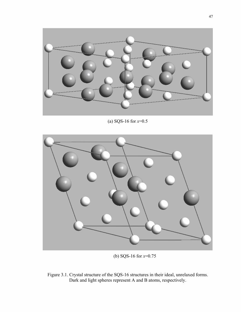
47
(a) SQS-16 for x=0.5
(b) SQS-16 for x=0.75
Figure 3.1. Crystal structure of the SQS-16 structures in their ideal, unrelaxed forms. Dark and light spheres represent A and B atoms, respectively.

48
Figure 3.2. Equilibrium lattice parameters of Mo-Nb bcc alloys as a function of
composition in comparison with the experimental data from Goldschmidt and Brand [57]
and Catterall and Barker [58].

49
Figure 3.3 Formation enthalpies of Mo-Nb bcc alloys as a function of composition in
comparison with the experimental data from Singhal and Worrell [56] and CPA
calculations from Sigli et al. [59].

50
Figure 3.4. Equilibrium lattice parameters of Ta-W bcc alloys as a function of
composition in comparison with the experimental data from Krishnan et al. [61] and CPA
calculations from Turchi et al. [62].
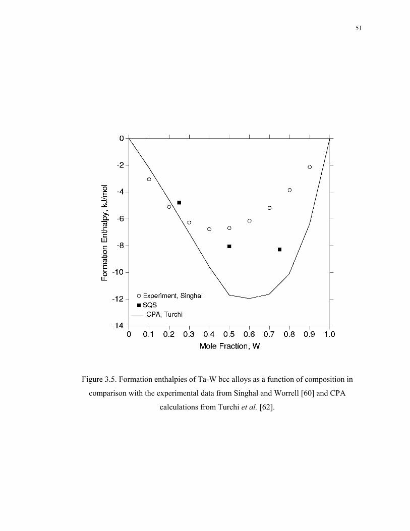
51
Figure 3.5. Formation enthalpies of Ta-W bcc alloys as a function of composition in
comparison with the experimental data from Singhal and Worrell [60] and CPA
calculations from Turchi et al. [62].
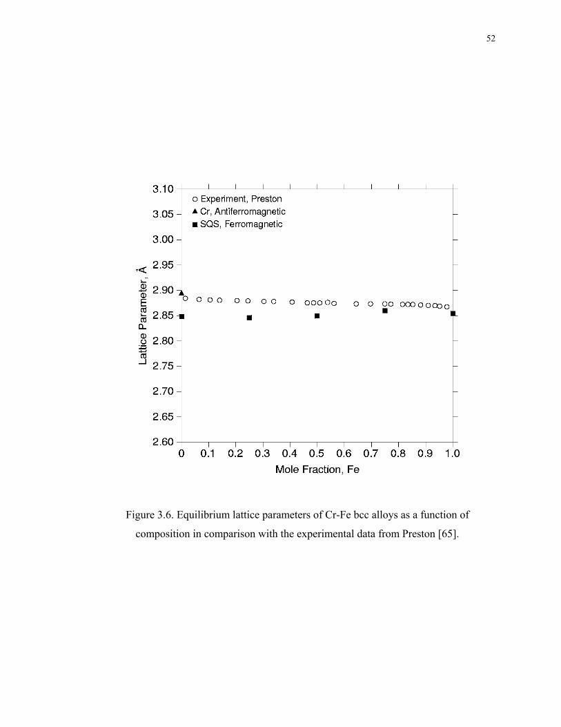
52
Figure 3.6. Equilibrium lattice parameters of Cr-Fe bcc alloys as a function of
composition in comparison with the experimental data from Preston [65].

53
Figure 3.7. Magnetic moment of Cr-Fe bcc alloys as a function of composition in
comparison with the experimental data from Aldred [66] and Dorofeyev et al. [67] and
CPA calculations from Kulikov and Demangeat [68].
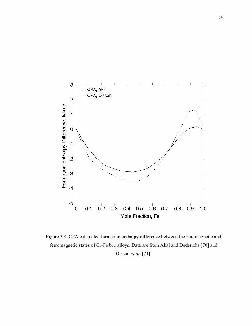
54
Figure 3.8. CPA calculated formation enthalpy difference between the paramagnetic and
ferromagnetic states of Cr-Fe bcc alloys. Data are from Akai and Dederichs [70] and
Olsson et al. [71].

55
Figure 3.9. Theoretical and experimental formation enthalpies of Cr-Fe bcc alloys as a
function of composition. The SQS paramagnetic results are obtained by adding the PMFMH →∆ from Akai and Dederichs [70] and Olsson et al. [71] to our SQS calculated
formation enthalpies of ferromagnetic Cr-Fe bcc alloys. Experimental data are from
Dench [69].

56
Figure 3.10. SQS calculated formation enthalpies of Nb-Mo, Ta-W and Cr-Fe bcc alloys
at x=0.5 as a function of N, the number of atoms per unit cell.

57
(a) Mo-Nb (b) Ta-W
(c) Cr-Fe
Figure 3.11. SQS calculated average nearest-neighbor bond lengths as a function of
composition in random (a) Mo-Nb, (b) Ta-W and (c) Cr-Fe bcc alloys. The dashed lines
represent the average lattice.
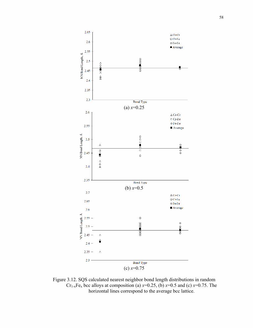
58
(a) x=0.25
(b) x=0.5
(c) x=0.75
Figure 3.12. SQS calculated nearest neighbor bond length distributions in random
Cr1-xFex bcc alloys at composition (a) x=0.25, (b) x=0.5 and (c) x=0.75. The horizontal lines correspond to the average bcc lattice.

59
Chapter 4. FIRST-PRINCIPLES STUDY OF THE AL-CU SYSTEM
4.1. First-Principles Method
First-principles calculations are performed using the plane wave method with Vanderbilt
ultrasoft pseudopotentials [46, 47], as implemented in the highly-efficient Vienna ab
initio simulation package (VASP) [48, 49]. Calculations using both the local density
approximation (LDA) and the generalized gradient approximation (GGA) are performed.
The k-point meshes for Brillouin zone sampling are constructed using the Monkhorst–
Pack scheme [52] and the total number of k-points times the total number of atoms per
unit cell is at least 6000 for all structures. A plane wave cutoff energy Ecut of 292.2 eV is
used for Al-Cu. According to our k-point and Ecut convergence tests, those parameters are
more than enough to guarantee that the total energies are converged to well within 1
kJ/mol.
All structures are fully relaxed with respect to the volume and shape of the unit cell as
well as all the internal atomic positions. By computing the quantum-mechanical forces
and stress tensor, structural and atomic relaxations are performed and all atoms are
relaxed into their equilibrium positions using a conjugate-gradient scheme. However,
when treating the Al-Cu bcc phase, there exist special difficulties associated with the
presence of structural instabilities: Al and Cu are stable in their fcc structure, but they are
both mechanically unstable in their bcc structure when tetragonally deformed along the
Bain path [72-74]. The total energy vs. c/a ratio curve exhibits a maximum at the bcc

60
structure (c/a=1), as shown in Figure 4.1. The bcc-based Al-Cu B2 structure is also found
to be unstable with respect to Bain distortions. Interestingly, the Al-Cu B2 structure
relaxes into fcc-based L10 with c/a=1.18, but not 1.414. This is because, for compounds,
some symmetry-dictated extrema in pure elements will be lost as the symmetry is now
determined by both structural parameters and atomic ordering [72, 73]. At higher
temperatures, the bcc phase in the Al-Cu system is stabilized due to the vibrational
entropy effect. Since all the present first-principles calculations are performed at T=0K
where the bcc lattice is unstable, we artificially “force” those bcc-based structures to stay
bcc by only relaxing their unit cell volumes but not the shape of the unit cell or the cell-
internal atomic positions.
4.2. Results
4.2.1. Formation Enthalpies of Compounds
The formation enthalpies of the stable and metastable phases in the Al-Cu system are
calculated by VASP in the present study using both LDA and GGA and the results are
summarized in Table 4.1. The experimental data and previous first-principles calculated
results in the literature are also included for comparison, when available. As shown, the
GGA results are in consistently better agreement with experiments. As the result, GGA
will be used in studying the Al-Cu system.

61
Very interestingly, contrary to the common belief that the energetic ground state of Al2Cu
is the θ phase, both the present LDA and GGA calculations show that θ′ is actually
energetically more stable than θ. This is in accordance with the conclusions arrived by
Wolverton and Ozolins [21]. Their calculations also show that the θ phase is stabilized at
higher temperatures due to its high vibrational entropy.
4.2.2. SQS Results
SQS calculations are also performed for the fcc and bcc phases (the 16-atom fcc SQS’s
are given in Appendix A). Due to issue of structural instabilities, we only relaxed the
volume of the bcc SQS’s. The results are also given in Table 4.1.
4.2.3. Cluster Expansions
The cluster expansions of Al-Cu fcc alloys have been constructed by Muller et al. [75]
using the full-potential linearized augmented plane-wave method (LAPW) and LDA.
Using their cluster expansions, Muller et al. [75] obtained the formation enthalpies of
random Al-Cu fcc alloys from Monte-Carlo simulations. In Figure 4.2, their results are
compared with the present SQS calculations with good agreements.
In this chapter, to validate our SQS results, we further construct the cluster expansions of
Al-Cu bcc alloys. The total energies of 45 bcc-based structures are calculated by VASP
using GGA. Due to the structural instabilities, only the unit cell volumes are relaxed.

62
Those total energies are then used by the MAPS code in ATAT [20, 44] to automatically
construct the cluster expansions of the Al-Cu bcc alloys. The final obtained pair and
multi-body ECI’s are shown in Figure 4.3. 9 pair interactions and 13 triple interactions
are used in constructing the cluster expansions. The large number of triple interactions is
necessary in order to account for the largely unsymmetrical formation enthalpies of the
Al-Cu bcc alloys. For example, ∆H(Al3Cu, D03)=0.25 kJ/mol while ∆H(AlCu3, D03)=-
21.1 kJ/mol. For sake of simplicity, the formation enthalpies of bcc-based structure in this
section are all referred to bcc Al and bcc Cu.
In Figure 4.5, the formation enthalpies of the bcc-based structures predicted from the
present cluster expansions are compared with the direct first-principles calculated results.
The root mean square error of our fit, defined as:
∑=
−=N
i
Calci
Fiti EE
NRMS
1
2)(1 (4.1)
is found to be 4.3 meV/atom, or 0.4 kJ/mol. The cross-validation score, which measures
the predictive power of the cluster expansions, is found to be 13.4 meV/atom, or 1.3
kJ/mol. It is defined as:
∑=
−=N
iii EE
NCV
1
2)(1 ) (4.2)

63
where iE is the calculated energy of structure i, while iE)
is the energy of structure i
predicted from a cluster expansion constructed using the energies of the other N-1
structures.
Finally, Monte-Carlo simulations are performed in a canonical ensemble using a
12x12x12 simulation cell. An extremely high temperature of 50000K is used to simulate
the truly random state of the alloy since at such high temperature, almost all the atom
exchanges in the Metropolis algorithm will be accepted. The final results are given in
Figure 4.6 in excellent agreement with the present SQS calculations.
4.3. Summary
In this chapter, the formation enthalpies of the stable and metastable phases in the Al-Cu
system are calculated by VASP using both LDA and GGA. SQS calculations are
performed for the Al-Cu fcc and bcc phases. The cluster expansions for the Al-Cu bcc
alloys are also constructed. For both Al-Cu fcc and bcc alloys, the SQS predicted
formation enthalpies of the random alloys agree rather well with the results obtained from
cluster expansions.

64
Table 4.1. First-Principles calculated formation enthalpies (in kJ/mol) of phases in Al-Cu system. The reference states are: fcc Al and fcc Cu.
Phases Space Group
VASP (LDA)
VASP (GGA)
FLAPW (LDA) Experiments
Al Bcc m3Im (229) 9.4 9.0 -
Cu Bcc m3Im (229) 3.9 3.4 -
θ″ (Al3Cu) P4/mmm (123) -10.3 -9.6 -9.3 [75] -
θ′ (Al2Cu) m3Fm (225) -20.8 -20.5 -19.2 [21] -
θ (Al2Cu) I4/mcm (140) -18.3 -16.2 -17.8 [21] -13.1 [76] -13.4 [77]
η2 (AlCu) C/2m (12) -24.0 -21.9 - -19.9 [76] -20.0 [77]
γ (Al4Cu9) 3m4P (215) -22.9 -20.7 - -20.3 [76]
Al0.75Cu0.25 - -5.1 [43] -5.9 -5.1 [75] -
Al0.5Cu0.5 - -9.6 [43] -9.5 - - Fcc SQS
Al0.25Cu0.75 - - -11.3 -11.5 [75] -
Al0.75Cu0.25 - - 7.3 - -
Al0.5Cu0.5 - - -0.3 - - Bcc SQS
Al0.25Cu0.75 - - -7.5 - -

65
-0.10
-0.05
0.00
0.05
0.10
0.15
0.20
0.6 0.8 1.0 1.2 1.4 1.6 1.8
c/a ratio
Tota
l ene
rgy
(eV
/ato
m)
AlCuAlCu
Figure 4.1. Total energy vs. c/a ratio along the tetragonal Bain path. c/a=1 corresponds to
bcc and c/a=1.414 corresponds to fcc.

66
-15000
-13000
-11000
-9000
-7000
-5000
-3000
-1000
1000
0.0 0.2 0.4 0.6 0.8 1.0
Mole Fraction, Cu
Form
atio
n En
thal
py, J
/mol
Cluster Expansions: Random
SQS
Figure 4.2. Formation enthalpies of random Al-Cu fcc alloys obtained from the present
SQS calculations in comparison with the cluster expansions results from Muller et al.
[75].
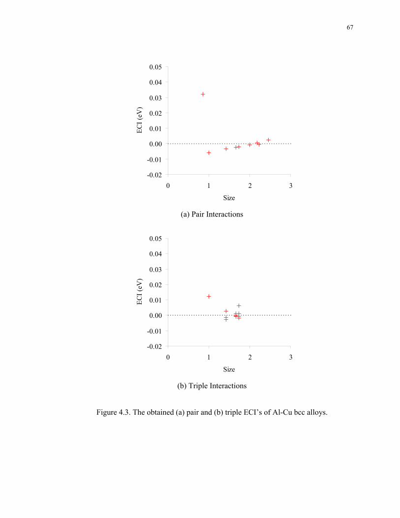
67
-0.02
-0.01
0.00
0.01
0.02
0.03
0.04
0.05
0 1 2 3
Size
ECI (
eV)
(a) Pair Interactions
-0.02
-0.01
0.00
0.01
0.02
0.03
0.04
0.05
0 1 2 3
Size
ECI (
eV)
(b) Triple Interactions
Figure 4.3. The obtained (a) pair and (b) triple ECI’s of Al-Cu bcc alloys.

68
-0.30
-0.25
-0.20
-0.15
-0.10
-0.05
0.00
0.05
0.0 0.2 0.4 0.6 0.8 1.0
Mole Fraction, Cu
Form
atio
n En
thal
py (e
V/a
tom
)
CalculatedFittedGround State
Figure 4.4. The calculated and fitted formation enthalpies of bcc-based structures as a
function of composition. The calculated ground state convex hull is also shown.

69
-0.30
-0.25
-0.20
-0.15
-0.10
-0.05
0.00
0.05
-0.30 -0.25 -0.20 -0.15 -0.10 -0.05 0.00 0.05
Calculated Formation Enthalpy (eV/atom)
Fitte
d Fo
rmat
ion
Enth
alpy
(eV
/ato
m)
Figure 4.5. Comparisons between calculated and fitted formation enthalpies.
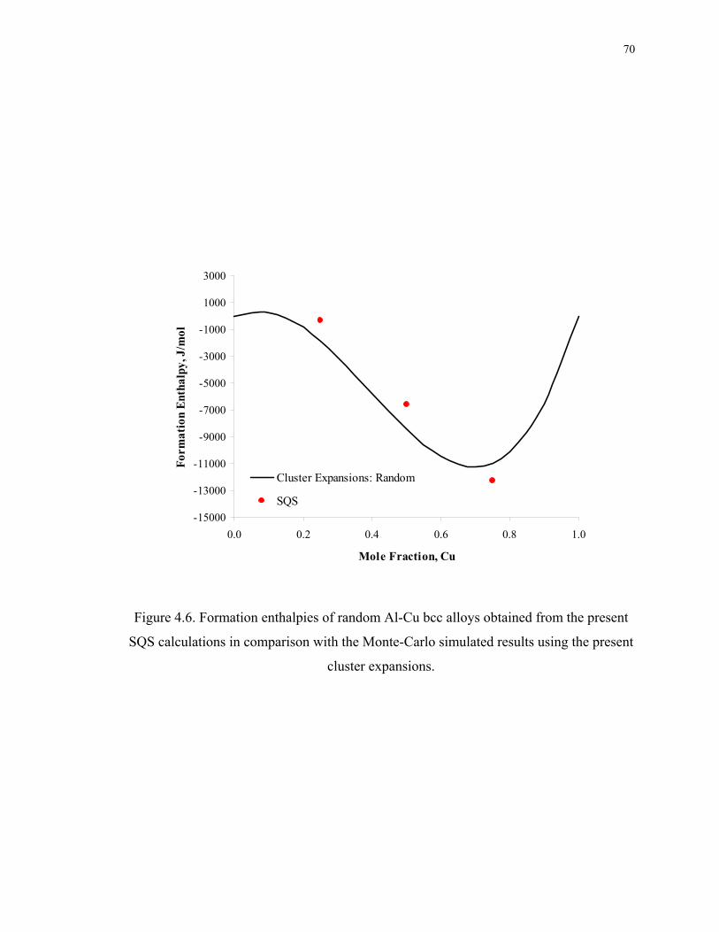
70
-15000
-13000
-11000
-9000
-7000
-5000
-3000
-1000
1000
3000
0.0 0.2 0.4 0.6 0.8 1.0
Mole Fraction, Cu
Form
atio
n En
thal
py, J
/mol
Cluster Expansions: Random
SQS
Figure 4.6. Formation enthalpies of random Al-Cu bcc alloys obtained from the present
SQS calculations in comparison with the Monte-Carlo simulated results using the present
cluster expansions.

71
Chapter 5. THERMODYNAMIC REMODELING OF THE AL-CU SYSTEM
INCOPORATING FIRST-PRINCIPLES ENERGETICS
5.1. Literature Review
A comprehensive review of the phase equilibria and thermochemical data of the Al-Cu
binary system has been given by Murray [78] and will not be repeated here. Following
are the new experimental data not included by Murray [78].
5.1.1. Phase Equilibrium Data
Recently, Liu et al. [79] reinvestigated the phase equilibria in the Al–Cu system over the
temperature range 500~1000°C and composition range 40~85at.% Cu using diffusion
couple, differential scanning calorimetry (DSC) and high temperature X-ray diffraction
(XRD) methods. Liu et al. [79]’s data are used in the present optimization process.
5.1.2. Thermochemical Data
Recently, Stolz et al. [80], Witusiewicz [81] and Kanibolotsky et al. [82] redetermined
the enthalpy of mixing of the liquid Al-Cu alloys using a high-temperature calorimeter.
Surprisingly, their data are much more negative than adopted by Murray [78]. The new
data by Stolz et al. [80] and Witusiewicz [81] are used in the present optimization
process.
72
5.2. First-Principles Data
The first-principles data in Chapter 4 are used in the present CALPHAD optimization
process together with the existing experimental thermochemical and phase equilibria
data. In addition, the vibrational formation entropies of θ and θ′ calculated by Wolverton
and Ozolin [21] using the linear-response theory [22] are also used.
5.3. Thermodynamic Modeling
5.3.1. Pure Elements
Solid Al and Cu both have the face-centered cubic (fcc) structure. The Gibbs energies of
pure Al and Cu in their stable, metastable and unstable states are directly taken from the
SGTE pure element database.
5.3.2. Solution Phases
The liquid, fcc and bcc phases are treated using substitutional solution model (Eq. (2.4)).
5.3.3. θ phase
The θ phase is described by an (Al)0.667(Al,Cu)0.333 two-sublattice model. Its Gibbs
energy per mole of formula units is written as:

73
CuAlAlIICu
IIAl
IICu
IICu
IIAl
IIAlCuAl
IICuAlAl
IIAlm
Lyy
yyyyRTGyGyG
,:
:: )lnln(333.0
+
+++= oo
(5.1)
where CuAlAlL ,: is the interaction parameter in the second sublattice.
5.3.4. The η and ε phase
The η and ε phase are described by an (Cu)0.5(Al,Cu)0.5 two-sublattice model. Its Gibbs
energy per mole of formula units is written as:
CuAlCuIICu
IIAl
IICu
IICu
IIAl
IIAlCuCu
IICuAlCu
IIAlm
Lyy
yyyyRTGyGyG
,:
:: )lnln(5.0
+
+++= oo
(5.2)
where CuAlCuL ,: is the interaction parameter in the second sublattice.
5.3.5. The γ0 and γ1 Phase
The γ0 and γ1 phase are described by an (Al)0.3077(Al,Cu)0.0769(Cu)0.6154 three-sublattice
model. Their Gibbs energies per mole of formula units are written as:
CuAlCuIICu
IIAl
IICu
IICu
IIAl
IIAlCuCuAl
IICuCuAlAl
IIAlm
Lyy
yyyyRTGyGyG
,:
:::: )lnln(0.0769
+
+++= oo
(5.3)

74
where CuCuAlAlL :,: is the interaction parameter in the second sublattice. kjiG ::o is the Gibbs
energy of the compound with the first sublattice entirely occupied by element i, the
second entirely by j, and the third entirely by k, be it real or hypothetical.
5.3.6. Stoichiometric Compounds
Compounds ξ-Al9Cu11, δ-Al2Cu3, θ′ and θ″ with negligible homogeneity ranges are
modeled as stoichiometric compounds in the present assessment. Their Gibbs energies
are expressed as:
BTAGxGxG fccCu
fccAl
CuAlm
xx +++−=− ooo )1(1 (5.4)
where A and B are the enthalpy and entropy of formation of the compound, respectively.
5.4. Optimization Procedures
Evaluation of the model parameters is performed using the PARROT program [83] in
Thermo-Calc [14], which works by minimizing the weighted sum of differences between
calculated and experimentally measured values using nonlinear least-square regression.
Different types of experimental data can be optimized simultaneously (the original input
file for Thermo-Calc used in the present assessment is listed in Appendix B). The weight
for each piece of experimental data is chosen according to its experimental uncertainty

75
and relative importance, and will be changed repeatedly during the assessment until most
of the experimental data are reasonably reproduced.
Since thermodynamic properties are generally explicitly related to model parameters, e.g.
the enthalpies of formation of liquid and solid phases, they are optimized first in the
present optimization. Phase equilibrium data, such as liquidus and invariant reaction
measurements, are then gradually incorporated into the optimization with more and more
model parameters introduced.
At the final stage of assessment, global optimization is performed. All parameters are
optimized simultaneously with all experimental data included, which ensures the best
possible agreement between model calculations and experimental data. The adjustments
of model parameters are rather small after the global optimization. The final obtained
model parameters are given in Table 5.1. The parameters from the COST 507 database
are also shown. In Table 5.2, the present optimized parameters are compared with the
first-principles results with good agreements. The final Thermo-Calc database file for Al-
Cu system is given in Appendix C.
5.5. Results and Discussions
Figure 5.1 shows the calculated formation enthalpy of the liquid phase using the present
model parameters in good agreement with experimental measurements. The calculated
activities of Al and Cu in liquid are also in good agreement with experiments, as shown
76
in Figure 5.2 and Figure 5.3. Figure 5.4 gives the calculated formation enthalpies of solid
phases at 298K. Figure 5.5 and Figure 5.6 also give the calculated formation enthalpies of
Al-Cu fcc and bcc solution phases in comparison with the experimental and first-
principles data. The agreements between model calculations, experimental measurements
and first-principles calculations are quite good, except for the bcc solution phase, where
large discrepancies exist between model calculations and first-principles results. We
attribute such large discrepancies to the mechanical instability of the bcc structure in Al-
Cu system rather than the failure of SQS. In fact, the large discrepancies between
CALPHAD and first-principles when treating unstable structures have been a long-
standing issue, as is discussed in a recent paper by Wang et al. [84].
Figure 5.7 shows the calculated Al-Cu phase diagram in comparison with experimental
measurements. All of the phase equilibria data are well reproduced. Figure 5.8 also gives
the blowup of the Al-rich and Cu-rich part of the calculated phase diagram. The θ′→θ
transition temperature is predicted in the present study to be 279K, somewhat lower than
the 423~473K temperature range predicted by Wolverton and Ozolins [21]. At such low
temperatures, although thermodynamically favorable, the θ′→θ transition is actually not
possible due to the extremely slow kinetics.
In Figure 5.9, the metastable solvus of θ′ and θ″ in Al-Cu system are calculated and
compared with experimental measurements. The calculated incoherent metastable fcc
miscibility gap is also shown. Very interestingly, even without considering the elastic
energy, the incoherent metastable fcc miscibility gap predicted in the present work is

77
already much lower than the experimentally measured GP-I Zone solvus, as shown in
Figure 5.9. This well suggests that GP-I zone formation in Al-Cu may not be due to the
metastable miscibility gap, the “traditional” explanation of GP-I zones, but rather due to
the metastable coherent ordering, as proposed by Wolverton [3].
It may be asked why the present model parameters and the COST 507 database give
similar equilibrium phase diagram but quite different metastable one, e.g. metastable fcc
miscibility gap. This is actually due to semi-empirical “fitting” nature of CALPHAD. In
the present study, with the integration of first-principles energetics into the CALPHAD
framework, the previously semi-empirical CALPHAD approach is now on solid physical
ground and its predictive power is greatly enhanced.

78
Table 5.1. Assessed thermodynamic parameters of the Al-Cu system (in SI units).
Phase Model Parameter Present COST 507 0LAl,Cu -66054+8.363T -66622+8.1T 1LAl,Cu 32489-8.524T 46800-90.8T+10TlnT Liquid (Al,Cu) 2LAl,Cu 7420-10.702T -2812 0LAl,Cu -43205-4.630T -53520+2T 1LAl,Cu 45224-6.789T 38590-2T Fcc (Al,Cu) 2LAl,Cu -16747+11.614T 1170 0LAl,Cu -73083+4.810T -73554+4T
Bcc (Al,Cu) 1LAl,Cu 48345-7.216T 51500-11.84T
AlAlG :o bcc
AlGo bccAlGo
∆GAl,Cu -16025+2.719T -15802+2.25T θ (Al)0.667(Al,Cu)0.333 0LAl:Al,Cu 0 737
θ′ (Al)0.667(Cu)0.333 ∆GAl,Cu -16783+5.434T -
θ″ (Al)0.75(Cu)0.25 ∆GAl,Cu -8389+0.385T -
ξ (Al)0.45(Cu)0.55 ∆GAl,Cu -21384+1.960T -21000+0.9T
δ (Al)0.4(Cu)0.6 ∆GAl,Cu -22278+1.702T -21340+0.6T
CuCuG :o bcc
CuGo bccCuGo
∆GCu:Al -20315+2.079T -20280+1.57T η (Cu)0.5(Al,Cu)0.5 0LCu:Al,Cu -17953 -12870-10T
CuCuG :o 22019+ fcc
CuGo bccCuGo
∆GCu:Al -20313+3.000T -18488+0.6T 0LCu:Al,Cu -29635-27.517T 3800-12T
ε (Cu)0.5(Al,Cu)0.5
1LCu:Al,Cu 0 -36000
∆GAl:Al:Cu -24185+31T-4TlnT -23132+30T-4TlnT γ1 (Al)0.3077(Al,Cu)0.0769(Cu)0.6154
∆GAl:Cu:Cu -20622+28.5T-4TlnT -21577+29.2T-4TlnT
∆GAl:Al:Cu -16339-4T -16866-3.5T γ0 (Al)0.3077(Al,Cu)0.0769(Cu)0.6154
∆GAl:Cu:Cu -15185-4.5T -15420-4.5T

79
Table 5.2. Comparisons between optimized parameters with first-principles calculated results. For the formation enthalpies, only GGA results are shown.
Phases Source ∆H (kJ/mol) ∆S (J/mol/K)
Present Assessment -16.0 -2.719 Al2Cu (θ)
First-Principles -16.2 (Present) -2.079 [21]
Present Assessment -16.8 -5.434 Al2Cu (θ′)
First-Principles -20.5 (Present) -5.155 [21]
Present Assessment -8.4 -0.385 Al3Cu (θ″)
First-Principles -9.6 (Present) -

80
Figure 5.1. The calculated enthalpy of formation of liquid in comparison with the
experimental data from Stolz et al. [80], Witusiewicz [81], Kanibolotsky et al. [82] and
Hultgren et al. [85]. Reference states: liquid Al and liquid Cu.

81
Figure 5.2. The calculated activities of Al in liquid at T=1073K in comparison with the
experimental data from Grube and Hantelmann [86]. Reference states: liquid Al.

82
Figure 5.3. The calculated activities of Al and Cu in liquid at T=1373K in comparison
with the experimental data from Hultgren et al. [87], Batalin et al. [88], Wilder [89] and
Matani and Nagai [90]. Reference states: liquid Al and liquid Cu.

83
Figure 5.4. The calculated formation enthalpies of Al-Cu solid phases at T=298.15K in
comparison with the experimental data from Hair and Downie [76] and Oelsen and
Middel [77]. The present VASP-GGA results are also shown. Reference states: fcc Al
and fcc Cu.

84
Figure 5.5. The calculated formation enthalpies of Al-Cu fcc alloys in comparison with
the experimental data from Hair and Downie [76] and Oelsen and Middel [77] and the
present first-principles SQS results. The cluster expansions results from Muller et al. [75]
are also included and shown as dash line. Reference states: fcc Al and fcc Cu.

85
Figure 5.6. The calculated formation enthalpies of Al-Cu bcc alloys in comparison with
the first-principles SQS results. The cluster expansions results from the present study are
also included and shown as dashed line. Reference states: bcc Al and bcc Cu.
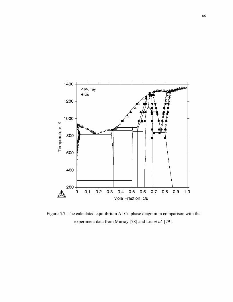
86
Figure 5.7. The calculated equilibrium Al-Cu phase diagram in comparison with the
experiment data from Murray [78] and Liu et al. [79].

87
(a) Al-rich corner
(b) Cu-rich corner
Figure 5.8. The (a) Al-rich and (b) Cu-rich corner of the calculated equilibrium Al-Cu
phase diagram in comparison with the experiment data from Murray [78] and Liu et al.
[79].

88
Figure 5.9. The calculated metastable θ′ and θ″ solvus of Al-Cu system in comparison
with the experiment solvus data from Beton and Rollason [26], Satyanarayana et al. [27],
Hori and Hirano [91] and Borelius et al. [92]. The incoherent metastable fcc miscibility
gap is also calculated and shown as dashed line.

89
Chapter 6. KINETIC MODELING OF CONSTITUTIONAL LIQUATION IN
AL-CU ALLOYS
6.1. Background
The mechanism of constitutional liquation was first proposed by Pepe and Savage [4] to
interpret the heat-affected zone (HAZ) hot cracking in weldments, a phenomenon
existing in many commercial alloy systems. It is defined as the sub-solidus, non-
equilibrium local eutectic melting of chemically heterogeneous regions of the matrix, e.g.
second-phase particles or inclusions. It is a non-equilibrium phenomenon in that at the
temperature where constitutional liquation occurs, the second phase and the liquid phase
are not stable in the alloy. However, due to the rapid heating rate experienced during
welding operations, the second-phase particles may not be dissolved completely at the
time the eutectic temperature is reached in the HAZ. Metastable liquid may thus nucleate
heterogeneously at the interfaces between the remaining second-phase particles and the
matrix, followed by rapid melting of the second-phase particles and part of the
surrounding matrix. After prolonged annealing, the metastable liquid droplets will slowly
dissolve back into the surrounding matrix, the rate of which is controlled by the volume
diffusion in the matrix.
In this chapter, the diffusion processes of both the solid-state dissolution and the
constitutional liquation in the model Al-Cu alloy system are computationally investigated
using the DICTRA program [15] coupled with critically assessed thermodynamic and

90
kinetic databases. In order to avoid constitutional liquation, all the second-phase particles
in the HAZ have to be completely dissolved before reaching the eutectic temperature
during the heating cycle. Based on this criterion, computer simulations were conducted
under the condition of constant heating rate to obtain the critical heating rates, beyond
which constitutional liquation will occur, for a series of Al-Cu alloys with different
compositions and θ (Al2Cu) precipitate sizes. The relationship between the microstructure
of an alloy and its critical heating rate is thus quantitatively established.
6.2. Literature Review
The solid-state dissolution and constitutional liquation of the θ phase in binary Al-Cu
alloys were experimentally studied by Reiso et al. [93] and Wilson [94]. In both studies,
samples consisting of intragranular θ precipitates dispersed in the Al-rich fcc (α) matrix
were rapidly heated to temperatures both below and above the eutectic temperature of
547°C, followed by isothermal holding at that temperature for various periods of time.
Their experimental conditions are listed in Figure 6.1. The samples were then air-cooled
by Reiso et al. [93] and water-quenched by Wilson [94]. Both used optical and SEM
microscopy coupled with quantitative image analysis tools to examine the area fraction
and surface number density of the θ particles and the eutectic regions in the quenched
samples. In both studies, particles on the grain boundaries were excluded from the
measurements. The chemical compositions of various phases were measured by Reiso et
al. [93] and Wilson [94] using wavelength dispersive spectrometer (WDS) and electron
probe microanalysis (EPMA), respectively.

91
In both studies, it was experimentally observed that at temperatures below the eutectic
temperature, i.e. 535°C and 546°C, only solid-state dissolution of the intragranular θ
precipitates in the α matrix occurred. While at temperatures above the eutectic
temperature but still below the solidus, i.e. 555°C, 565°C and 585°C, the θ precipitates
melted rapidly (~1 second) together with part of the surrounding α matrix, producing
spherical liquid droplets in the matrix. After sufficiently long annealing, the liquid
droplets were redissolved by the surrounding matrix and the final microstructure
consisted of single-phase α grains only.
However, in Reiso et al. [93]’s air-cooled samples annealed at 555°C, most liquid
droplets solidified into lamellar eutectic structures, only few particles were featureless,
i.e. without any internal structure. While in Wilson [94]’s water-quenched samples, vast
majority of the solidified droplets appeared uniform in contrast and had no internal
structure. Only few exhibited lamellar eutectic structure. Reiso et al. [93] found the
compositions of the particles without internal structure always to be 54 wt.% Cu,
indicating that they are pure θ particles. This was confirmed by Chattopadhyay et al.
[95]’s microhardness measurements in their study of the solidification behavior of the Al-
Cu liquid droplets embedded in an α matrix. However, Wilson [94] measured the
composition of the solidified droplets with no internal structure to be 45.5±2.2 wt.% Cu,
much lower than the expected 54 wt.% Cu. This may be due to the inadvertent
contributions from the surrounding α matrix when doing EPMA measurements since the
θ particles in Wilson [94]’s study are rather small.

92
As shown in Figure 6.1, the measured eutectic compositions in Reiso et al. [93]’s
samples fall in a range from 35 to 43 wt.% Cu with a weighted average of 38.25 wt.%
Cu, considerably higher than the anticipated equilibrium eutectic composition of 33 wt.%
Cu. From the calculated metastable α liquidus shown in Figure 6.2, this average
composition of 38.25 wt.% Cu corresponds to a large undercooling of 27°C of the liquid
phase. Chattopadhyay et al. [95] and Kim and Cantor [96] both experimentally measured
the undercooling of liquid droplets embedded in an α matrix. Their experimental results
are given in Table 6.2. As can be seen, present prediction of the undercooling agrees well
with the experimental observations.
The large undercooling of liquid below the eutectic temperature indicates a difficulty of
heterogeneous nucleation of the θ precipitates at the α/liquid interface during
solidification. As the liquid droplets undercool below the eutectic temperature without
nucleation of the θ phase, the α phase continues to grow epitaxially from the pre-existing
matrix, i.e. with the same crystal orientation as the matrix, and consumes part of the
liquid phase. The compositions of the liquid droplets and the newly formed α phase will
follow the metastable α liquidus and solidus (see Figure 6.2), respectively, in order to
maintain local equilibrium at the α/liquid interface. As the liquid droplets decrease in
size, they get more and more enriched in Cu. At some critical undercooling, the θ phase
forms, and the remaining liquid droplets solidify either into a lamellar eutectic structure
or into a divorced eutectic structure in which the newly formed α phase grows on the α
matrix. As newly formed α phase has a higher Cu concentration, as shown in Figure 6.2,
there must exist a Cu concentration gradient in the matrix surrounding the solidified

93
particles. This has been experimentally observed by Reiso et al. [93] and Chattopadhyay
et al. [95] using aging technique and by Wilson [94] using secondary electron and Cu-Kα
x-ray mapping. Wilson [94] also determined the composition of the Cu-rich region
surrounding the solidified θ particles in the matrix to be 5.2 wt.% Cu.
However, in Reiso et al. [93]’s experiment in which a sample was quenched in air
slightly before the temperature 555°C was reached, the compositions of the eutectic
particles are always in the range of 32-34 wt.% Cu, i.e. around the equilibrium eutectic
composition of 33 wt.% Cu. This is because in this sample, the θ particles were only
partially melted and therefore eliminated the need for new nucleation of the θ phase
during solidification. The liquid thus solidified into a coarse eutectic structure without
any undercooling. It was observed that nucleation of liquid tends to start heterogeneously
at the end of the lenticular θ particles. This can be well understood from the classical
nucleation theory since the α/θ interfacial energy is higher at those parts, and therefore
lower energy barrier for liquid nucleation.
6.3. Computer Modeling
6.3.1. Thermodynamic Data
For studying constitutional liquation in Al-Cu system, the existing COST 507 [23]
database suffices since only the Gibbs energies of fcc, liquid and θ phases are needed.
Their Gibbs energies can be found in Table 5.1.

94
Figure 6.2 shows the Al-rich corner of the Al-Cu phase diagram calculated by Thermo-
Calc. The Gibbs energy curves of liquid, fcc and θ phases at 565°C are plotted in Figure
6.3. The thermodynamic driving force ∆G for constitutional liquation reaction θ + α =
Liquid is graphically shown in Figure 6.3 and calculated as a function of temperature in
Figure 6.4, which is approximately a linear function of temperature and is zero at the
eutectic point.
6.3.2. DICTRA Simulations
Sharp-Interface model, combined with local equilibrium assumption, proves to be a very
powerful tool for the simulation of diffusion-controlled phase trans-formations. The
finite-difference code DICTRA [15], a program for simulating one-dimensional
diffusion-controlled phase transformations in multi-component alloy systems, was used
in the present work. Only simple geometries, i.e. planar, cylindrical or spherical, can be
treated. DICTRA is interfaced with Thermo-Calc [14], which handles all the
thermodynamic calculations needed by DICTRA, e.g. thermodynamic factors for
calculating interdiffusion coefficients and local equilibrium conditions at the phase
interfaces. As illustrated in Figure 6.5, typical DICTRA simulations are performed in the
following four steps:
1) Calculate the local thermodynamic equilibrium at the phase interface.
2) Solve the multi-component diffusion equations using the finite-difference method.
3) Solve the flux balance equations and obtain the interfacial velocity.
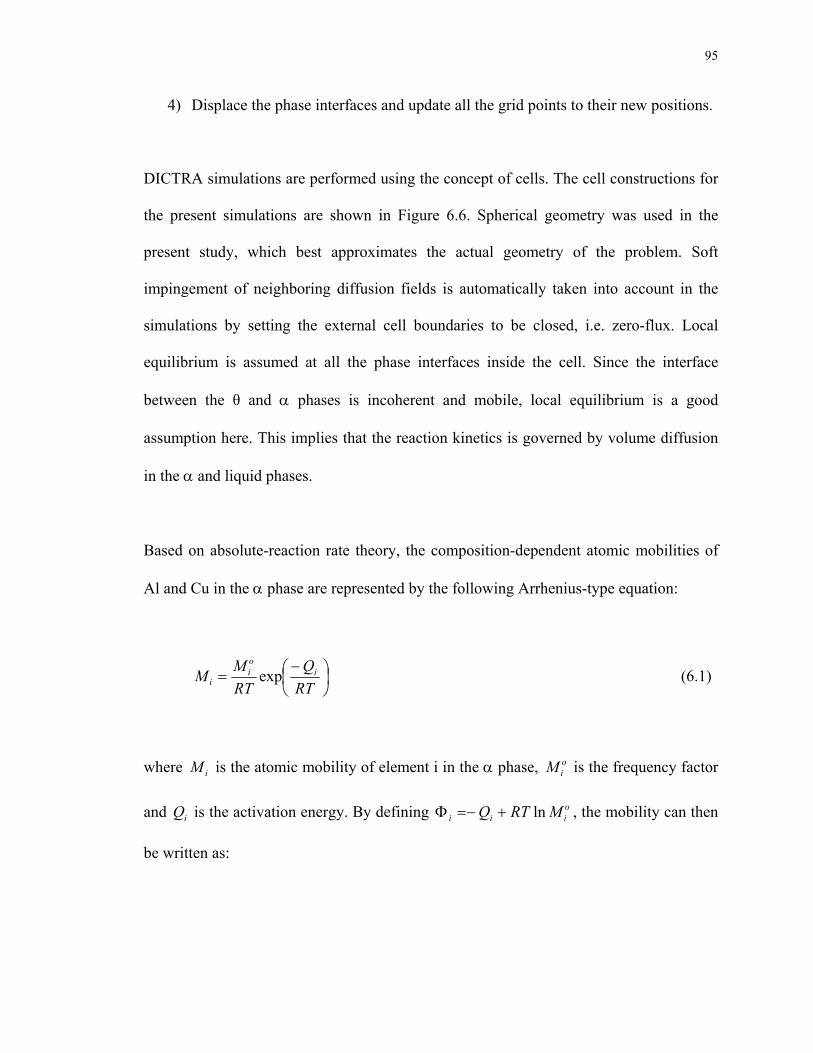
95
4) Displace the phase interfaces and update all the grid points to their new positions.
DICTRA simulations are performed using the concept of cells. The cell constructions for
the present simulations are shown in Figure 6.6. Spherical geometry was used in the
present study, which best approximates the actual geometry of the problem. Soft
impingement of neighboring diffusion fields is automatically taken into account in the
simulations by setting the external cell boundaries to be closed, i.e. zero-flux. Local
equilibrium is assumed at all the phase interfaces inside the cell. Since the interface
between the θ and α phases is incoherent and mobile, local equilibrium is a good
assumption here. This implies that the reaction kinetics is governed by volume diffusion
in the α and liquid phases.
Based on absolute-reaction rate theory, the composition-dependent atomic mobilities of
Al and Cu in the α phase are represented by the following Arrhenius-type equation:
−=
RTQ
RTMM i
oi
i exp (6.1)
where iM is the atomic mobility of element i in the α phase, oiM is the frequency factor
and iQ is the activation energy. By defining oiii MRTQ ln+−=Φ , the mobility can then
be written as:

96
Φ=
RTRTM i
i exp1 (6.2)
In the spirit of the CALPHAD approach, the composition-dependence of iΦ is expressed
in a form similar to Eq. (2.4):
( )∑=
−Φ+Φ+Φ=Φn
k
kCuAl
CuAli
kCuAl
CuiCu
AliAli xxxxxx
0
, (6.3)
where jiΦ is the mobility parameter of element i in pure j, taken from the DICTRA
MOB2 database and shown in Table 6.3. CuAli
k ,Φ are the interaction parameters for
element i and are zero for both Al and Cu.
The composition-dependent interdiffusion coefficient in the α phase can then be
calculated using Darken’s equation:
2
2
)(~Cu
mCuAlAlCuCuAl dx
GdxxMxMxDα
+= (6.4)
In lack of experimental information, the interdiffusion coefficient in the liquid phase was
assumed to have a constant value of 10-9 m2/s. Diffusion in the θ phase was neglected in
all present simulations.

97
6.4. Results
6.4.1. Simulation of Isothermal Holding
Table 6.4 gives the initial conditions for DICTRA simulations used in the present study
to reproduce Wilson [94] and Reiso et al. [93]’s experimental conditions. The initial
compositions in the θ and α phase were set to be uniform. The average θ particle radius
θr was reported by Wilson to be 1.65µm. θr in the study by Reiso et al. was estimated as
follows:
ANfr
πθ
θ 23
= (6.5)
where θf and AN are the measured volume fraction and surface number density of θ
listed in Table 6.1, respectively. The thickness of the surrounding α matrix was
calculated by mass balance such that the overall composition corresponds to that of the
alloy.
Using the initial conditions given in Table 6.4, the isothermal solid-state dissolution of
the θ phase at 535°C and 546°C without liquation were simulated. The simulated results
agree very well with experimental data, as shown in Figure 6.7 to Figure 6.9. As a further
check of the validity of the present simulations, the compositional profile in the α matrix
on both sides of a dissolving θ plate was simulated by DICTRA and compared with Hall

98
[97]’s experimental observations. As shown in Figure 6.10 and Figure 6.11, the
agreement with experiments is quite good.
Constitutional liquation at 555°C, 565°C and 585°C, all below the solidus but above the
eutectic temperature, were then simulated. The concentration profiles during
constitutional liquation at 565°C are shown in Figure 6.12 with arrows indicating the
direction of interface movement at different times. As can be seen from the simulation,
within 1 second, the θ particle transformed into the liquid phase together with part of the
surrounding α matrix and the liquid composition quickly homogenized to the equilibrium
liquidus composition. As soon as the composition of the liquid phase reached the liquidus
composition, the liquid phase began to shrink, the rate of which is controlled by the
diffusion rate of Cu in the α matrix. The same is true for the other two temperatures. The
variations of liquid volume fractions with time are also plotted in Figure 6.13 to Figure
6.15 for the three different temperatures with the experimental data superimposed. It
seems that DICTRA simulations give higher liquid volume fractions than those observed
by experiments. This large discrepancy is due to the fact that all experimental
measurements of the high temperature liquid volume fractions were made on solidified
microstructures. However, the actual size and morphology of the liquid as it existed at the
annealing temperature may be changed dramatically during cooling. The final solidified
microstructure depends both on the cooling rate and the nucleation of the θ phase. As
schematically shown in Figure 6.16, first the proeutectic α' will grow epitaxially from the
pre-existing matrix, decreasing the size of the liquid phase and make it more and more
enriched in Cu. At some critical undercooling, the remaining liquid droplets L' may either

99
solidify into a lamellar eutectic structure αE + θE, as in Reiso et al. [93]’s case, or into a
divorced eutectic structure α" + θ, as in Wilson [94]’s case. In quantifying the solidified
liquid droplet volume fraction, only those regions in the matrix delineated by the θ
particles, i.e. lamellar eutectic structures and pure θ precipitates, are actually measured
since both α" and the proeutectic α' are physically and optically indistinguishable from
the pre-existing α matrix.
In order to compare the DICTRA simulated results with the experimental measurements
by Reiso et al. [93], the solidification of liquid from the annealing temperature of 555°C
after isothermal holding at that temperature for 1, 10 and 100 seconds was simulated
suppressing formation of the θ phase. A cooling rates of 1°C/sec was used to mimic the
air-cooling conditions by Reiso et al. [93]. The simulated results are given in Figure 6.17
together with results from Scheil simulation by Thermo-Calc [14], which assumes infinite
fast diffusion in the liquid and no diffusion in the solid. A high cooling rate of 100°C/sec
was also simulated to reproduce Wilson [94]’s water-quenching condition. However, this
gives results identical to those from Scheil simulation, as expected. In Figure 6.18, the Cu
concentration profiles during the solidification of the liquid phase are also shown at 0, 20
and 40 seconds after 10 seconds of isothermal holding at 555°C. As can be seen, the
liquid phase decreases in size with time and at the same time get more and more enriched
in Cu. Using the average eutectic composition of 38.25 wt.% Cu from Reiso et al. [93], it
can be obtained from Figure 6.17 that about 71 percent of original liquid at annealing
temperature of 555°C transformed into eutectic structure, the rest goes to proeutectic α'.
Therefore, Reiso et al. [93]’s experimental data at 555°C were divided by a factor of 0.71

100
and compared with DICTRA simulations in Figure 6.19. A good agreement was observed
after the correction.
As for Wilson [94]’s case, most liquid droplets in the water-quenched samples solidified
into a structure consisting of proeutectic α' and divorced eutectic α" + θ, as shown in
Figure 6.16(b). Since DICTRA and Scheil simulations give the same results for the case
of high cooling rate, for simplicity, Scheil simulations were performed using Thermo-
Calc to simulate the solidification of liquid from annealing temperature 565°C and 585°C
without formation of the θ phase, respectively. The starting composition of the liquid
phase was set to be the equilibrium liquidus composition at the respective annealing
temperature. Figure 6.20 shows the simulated volume fraction of liquid transformed into
proeutectic α', 'αf , with respect to the liquid undercooling at both temperatures. At some
critical undercooling, the remaining liquid L' then transformed into divorced eutectic α"
+ θ. Using the level rule, the volume fraction of liquid actually transformed into the θ
phase, Lfθ , can thus be calculated as follows:
"
"'' )1(
αθ
ααθ xx
xxff LL
−−
−= (6.6)
where 'Lx and "αx are the mole fraction of Cu in L' and α", and can be read from the
metastable liquidus and solidus in Figure 6.2 for a given undercooling, respectively. θx is
the mole fraction of Cu in the θ phase and has a value of 0.333. In Figure 6.21, Lfθ is
plotted as a function of liquid undercooling for both temperatures. It can be seen that the

101
value of Lfθ is almost constant over a large range of undercooling. In our calculations, we
assume the same undercooling as in Reiso et al. [93]’s case, i.e. 27°C. The final results
are given in Table 6.5. Wilson [94]’s experimental data at 565°C and 585°C were then
divided by the corresponding Lfθ value in Table 6.5 and compared with DICTRA
simulations in Figure 6.22 and Figure 6.23, respectively. Both DICTRA simulations
agree very well with experimental measurements after the correction.
6.4.2. Simulation of Continuous Heating
The critical heating rate to avoid constitutional liquation was further studied through
DICTRA simulations. The initial compositions and volume fractions of the α and θ
phases were calculated by Thermo-Calc at the room temperature for a series of alloys
with composition 1, 2, 3, 4 and 5 wt.% Cu, which serve as inputs to DICTRA
simulations. A linear heating profile, i.e. T=25°C+κt, was used in the present study
though other types of nonlinear heating profiles can also be used. Here t is time in
seconds and κ is the constant heating rate (°C/sec). The critical heating rate can thus be
defined as the maximum κ at which the θ particle is completely dissolved into the matrix
before the eutectic temperature is reached. Simulations are then performed for each alloy
by choosing different initial precipitate sizes for the θ particle and different constant
heating rates. The obtained critical heating rate for each alloy is plotted as a function of
the precipitate size in Figure 6.24. A linear relationship is observed when we use the
logarithmic scale for both axes. Using linear regression, it is found that the critical
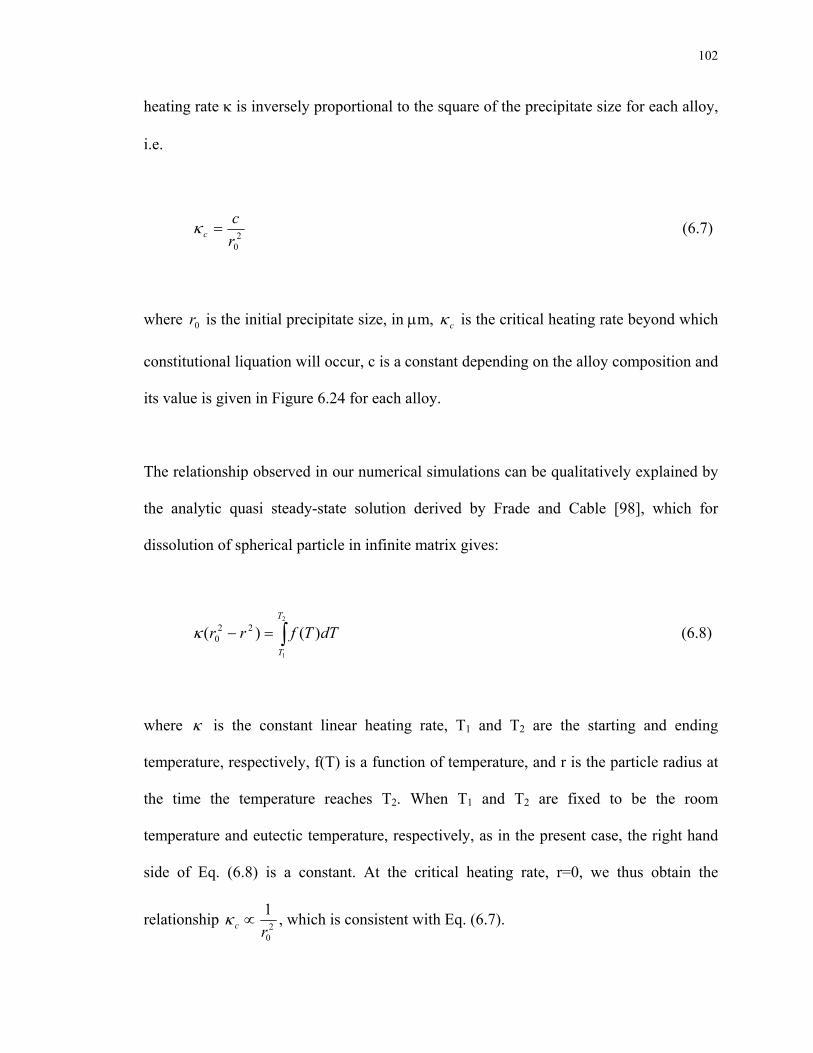
102
heating rate κ is inversely proportional to the square of the precipitate size for each alloy,
i.e.
20rc
c =κ (6.7)
where 0r is the initial precipitate size, in µm, cκ is the critical heating rate beyond which
constitutional liquation will occur, c is a constant depending on the alloy composition and
its value is given in Figure 6.24 for each alloy.
The relationship observed in our numerical simulations can be qualitatively explained by
the analytic quasi steady-state solution derived by Frade and Cable [98], which for
dissolution of spherical particle in infinite matrix gives:
∫=−2
1
)()( 220
T
T
dTTfrrκ (6.8)
where κ is the constant linear heating rate, T1 and T2 are the starting and ending
temperature, respectively, f(T) is a function of temperature, and r is the particle radius at
the time the temperature reaches T2. When T1 and T2 are fixed to be the room
temperature and eutectic temperature, respectively, as in the present case, the right hand
side of Eq. (6.8) is a constant. At the critical heating rate, r=0, we thus obtain the
relationship 20
1rc ∝κ , which is consistent with Eq. (6.7).

103
6.5. Summary
In this chapter, all stages of constitutional liquation were simulated by DICTRA using
realistic thermodynamic and kinetic databases. Quantitative agreement had been observed
between computer simulations and experimental observations. The relationship between
the high temperature liquid droplets and the room temperature solidified microstructure
was quantitatively clarified in this study through the consideration that the liquid droplets
can either transform into the lamella structure or into the divorced eutectic structure
during solidification. The computational procedures for obtaining the critical heating rate
to avoid constitutional liquation are demonstrated. We conclude that, constitutional
liquation depends both on the heating rate and the average precipitate size in the HAZ.
Rapid heating rate and large precipitate size will both promote constitutional liquation.
The critical heating rate for avoiding liquation was simulated and found to be inversely
proportional to the square of the precipitate size. The present computational procedures
can be readily extended to predict the susceptibility of multicomponent commercial
alloys to constitutional liquation during welding with available thermodynamic and
kinetic databases.

104
Table 6.1. Experimental conditions. Composition (wt.% Cu)
Source Total θ α
θ Volume
Fraction
θ Surface Density
(1/µm2)
Temperature
(°C)
Reiso [93] 4.2 54 3.1 0.015 0.00020 546, 555
Wilson [94] 3.2 52.6 1.7 0.0217 0.00272 535, 565, 585
Table 6.2. Experimental measurements of liquid undercooling.
Source Alloy Composition
(wt.% Cu)
Cooling Rate
(°C/min)
Undercooling (°C)
∆T=Teut-T
Chattopadhyay [95] 3.8 4-7 19-28
Kim and Cantor [96] 7 0.5-20 16-25
Table 6.3 Kinetic parameters of the Al-Cu system. Activation energies are in J/mol and frequency factors are in m2/s, T is in K.
Fcc: (Al,Cu)
Mobility of Al
)1071.1ln(142000 4−×+−=Φ RTAlAl
)108ln(181300 6−×+−=Φ RTCuAl
Mobility of Cu
)1047.6ln(135100 5−×+−=Φ RTAlCu
)1059.2ln(201000 5−×+−=Φ RTCuCu

105
Table 6.4. Initial conditions for DICTRA simulations. Composition (wt.% Cu) Size (µm)
Study θ α θr αw
Temperature
(°C)
Reiso [93] 54 3.1 5.98 18.13 546, 555
Wilson [94] 54 1.48a 1.65 4.15 535, 565, 585 aCalculated by Thermo-Calc
Table 6.5. Values used to calculate the volume fraction of liquid transformed into θ.
Mole Fraction of Cu Volume Fraction Temperature
(°C) Lx 'Lx "αx θx 'αf
Lfθ 565 0.1518 0.2076 0.0429 0.333 0.31 0.392
585 0.1231 0.2076 0.0429 0.333 0.456 0.309

106
35 36 37 38 39 40 41 42 430
0.05
0.1
0.15
0.2
0.25
Weight Percent of Cu in Eutectic
Freq
uenc
y
Figure 6.1. Histogram showing the frequency distribution of composition of eutectic
particles from the measurements by Reiso et al. [93] Weighted average is 38.25 wt.% Cu.
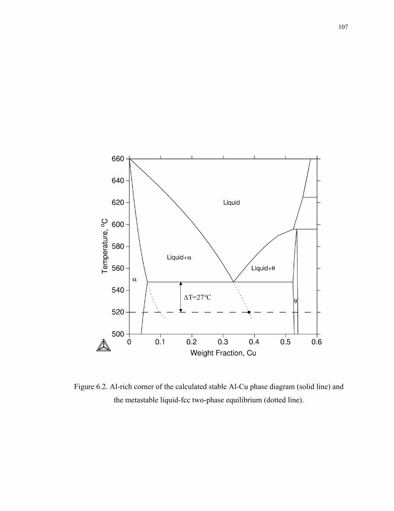
107
∆T=27°C∆T=27°C
Figure 6.2. Al-rich corner of the calculated stable Al-Cu phase diagram (solid line) and
the metastable liquid-fcc two-phase equilibrium (dotted line).

108
∆G∆G
Figure 6.3. Gibbs energy curves of various phases in the Al-Cu system at 565°C. The
driving force ∆G for constitutional liquation is also shown.

109
Figure 6.4. Thermodynamic driving force for constitutional liquation in the Al-Cu system
calculated using the COST 507 database.
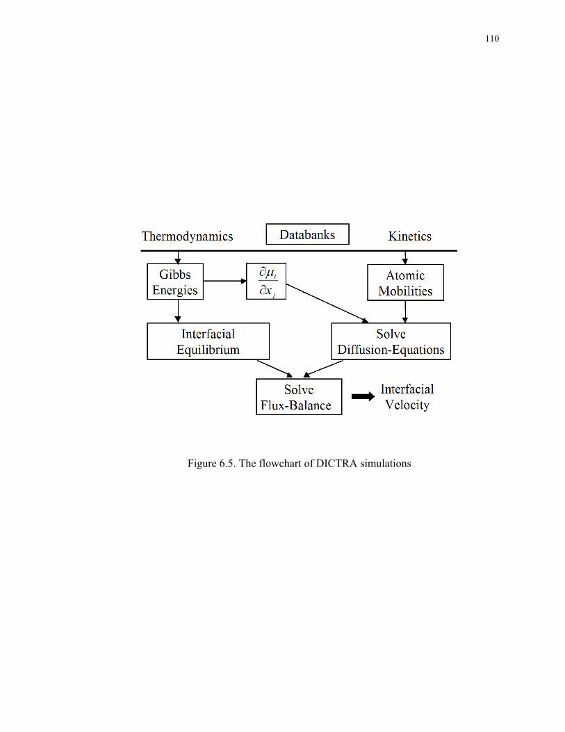
110
Figure 6.5. The flowchart of DICTRA simulations

111
θ
α
rθ wαθ
α
rθ wα
(a) Solid-state dissolution
θ
α
Liquid
θ
α
Liquid
(b) Constitutional liquation
Figure 6.6. Cell setup used in DICTRA simulations.

112
Figure 6.7. Simulated volume fraction of θ as a function of time during solid-state
dissolution of θ at 535°C in comparison with the experimental data from Wilson [94].

113
Figure 6.8. Simulated radius of the θ particles as a function of time during solid-state
dissolution of θ at 535°C in comparison with the experimental data from Wilson [94].
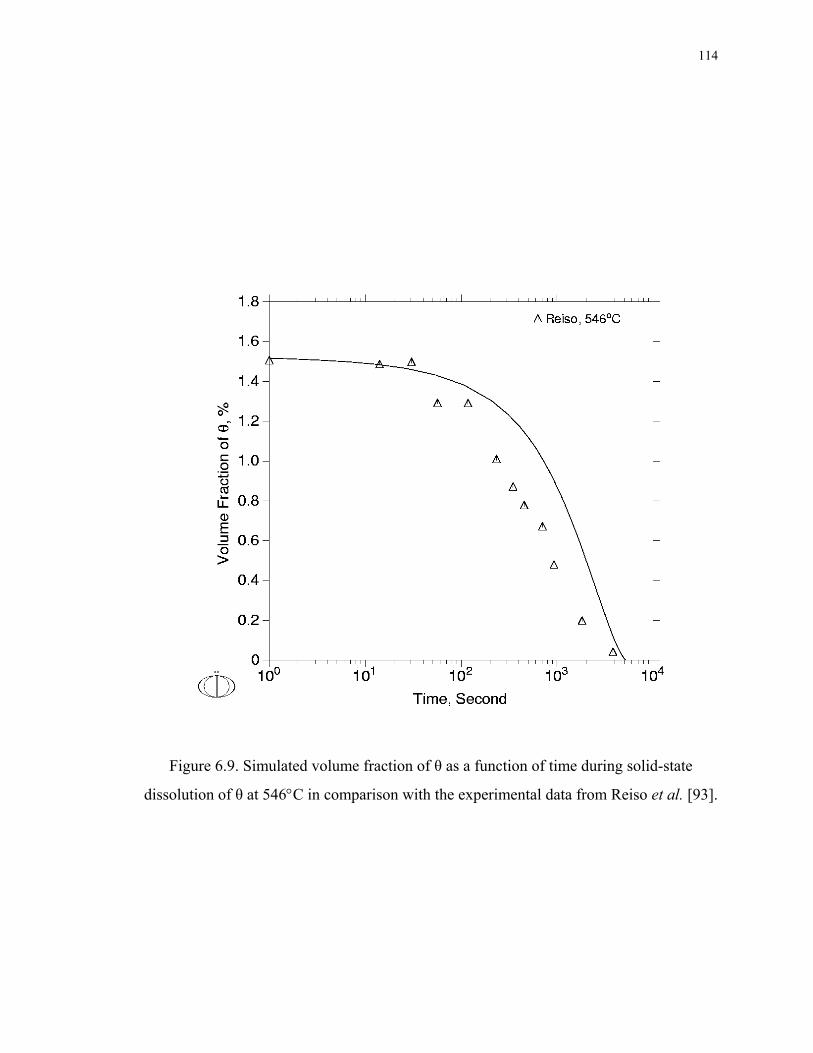
114
Figure 6.9. Simulated volume fraction of θ as a function of time during solid-state
dissolution of θ at 546°C in comparison with the experimental data from Reiso et al. [93].
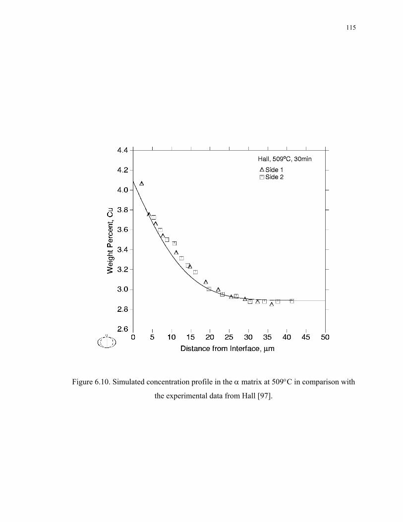
115
Figure 6.10. Simulated concentration profile in the α matrix at 509°C in comparison with
the experimental data from Hall [97].

116
Figure 6.11. Interfacial displacement as a function of time at 509°C and at 541°C in
comparison with the experimental data from Hall [97].

117
θ/liquid interface
Equilibrium
Liquid/α interface
2000s 1s
0.01s Initial
Figure 6.12. Concentration profiles during constitutional liquation at 555°C.

118
Figure 6.13. Simulated volume fraction of liquid as a function of time during
constitutional liquation at 555°C in comparison with the experimental data from Reiso et
al. [93].

119
Figure 6.14. Simulated volume fraction of liquid as a function of time during
constitutional liquation at 565°C in comparison with the experimental data from Wilson
[94].
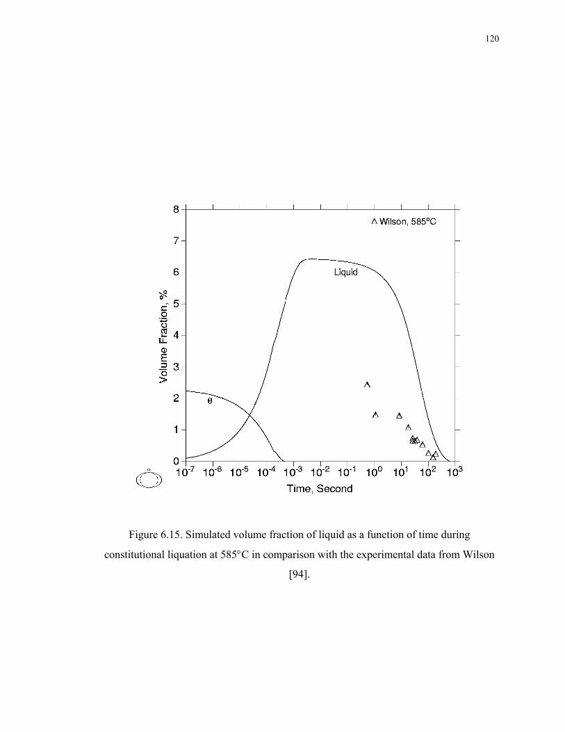
120
Figure 6.15. Simulated volume fraction of liquid as a function of time during
constitutional liquation at 585°C in comparison with the experimental data from Wilson
[94].

121
α
L
α
L'
α'
α
α'
θ
α"α'
α
αE
θE
α
L
α
LL
α
L'
α'
α
L'
α'
α
α'
θ
α"
α
α'
θ
α"α'
α
αE
θE
α'
α
αE
θE
(a) Lamellar eutectic (b) Divorced eutectic
Figure 6.16. Solidification microstructure of liquid droplets.

122
Figure 6.17. Scheil and DICTRA simulation of solidification of liquid from 555°C
without formation of the θ phase.

123
Figure 6.18. DICTRA simulation of solidification of liquid from 555°C without
formation of the θ phase. Cooling Rate equals to 1°C/sec.
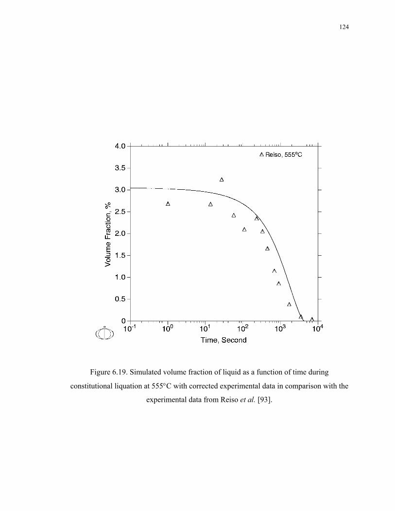
124
Figure 6.19. Simulated volume fraction of liquid as a function of time during
constitutional liquation at 555°C with corrected experimental data in comparison with the
experimental data from Reiso et al. [93].
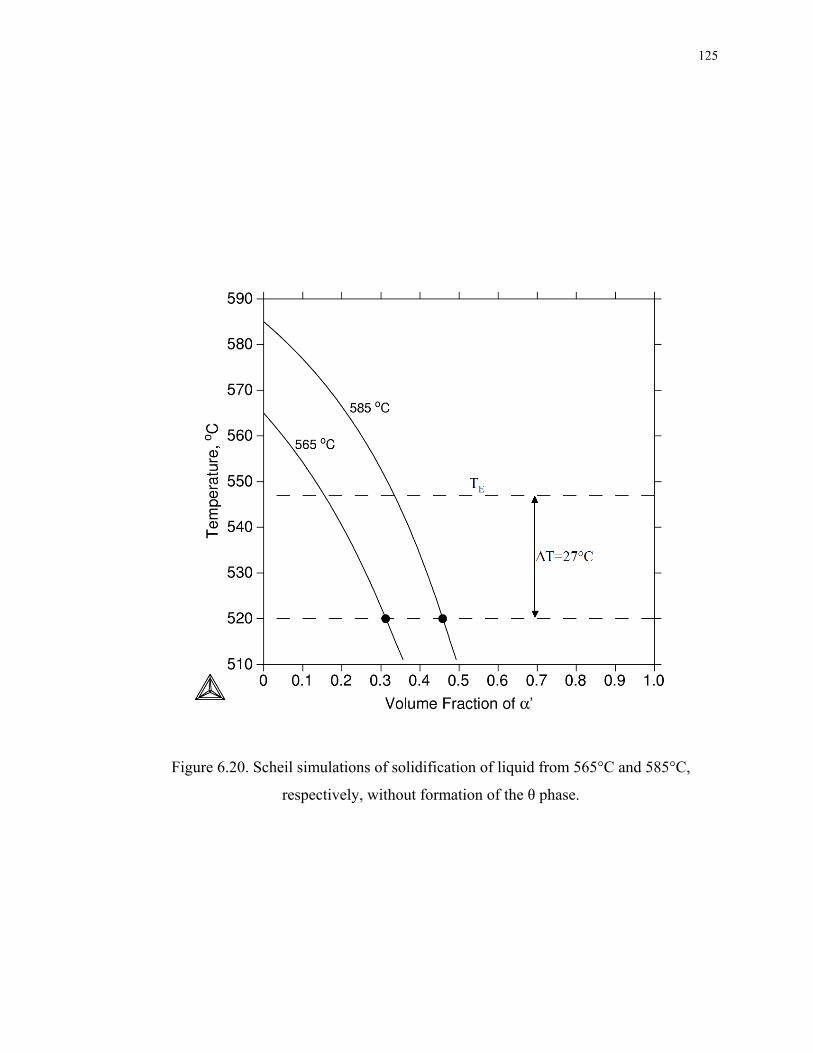
125
Figure 6.20. Scheil simulations of solidification of liquid from 565°C and 585°C,
respectively, without formation of the θ phase.

126
Figure 6.21. Calculated fraction of liquid transformed into θ with respect to undercooling.

127
Figure 6.22. Simulated volume fraction of liquid as a function of time during
constitutional liquation at 565°C with corrected experimental data in comparison with the
experimental data from Wilson [94].

128
Figure 6.23. Simulated volume fraction of liquid as a function of time during
constitutional liquation at 585°C with corrected experimental data in comparison with the
experimental data from Wilson [94].

129
Figure 6.24. Simulated results showing the susceptibility of a series of Al-Cu alloys
to constitutional liquation as a function of heating rate and particle size.

130
Chapter 7. FIRST-PRINCIPLES STUDY OF POINT DEFECTS IN B2 NIAL
7.1. The SQS Approach
The brute-force way to treat non-stoichiometric compounds with concentrated point
defects would be to construct a large supercell and randomly distribute the point defects
on the host lattice. This would necessarily require very large supercells to adequately
mimic the compositional disorder caused by the significant number of point defects.
Since density functional methods are computationally constrained by the number of
atoms that one can treat, such an approach could be computationally prohibitive.
Therefore, in the present study, we adopt the Special Quasirandom Structure (SQS)
approach [34, 35] to model the B2 alloys. In Chapter 3, SQS’s for the simple binary bcc
alloys have already been developed. In this chapter, we further develop various SQS
structures for random pseudobinary A1-xBxC B2 alloys. Here A and B are randomly
distributed on one sublattice with the second sublattice completely occupied by C, and
thus the substitutional alloy problem is simple-cubic-based [99]. Assuming that only one
type of constitutional point defects is present in the maximally ordered state [100] of the
non-stoichiometric alloy, as is the case for B2 NiAl, we treat the Al-rich and Ni-rich B2
NiAl as Ni1-xVaxAl and Al1-xNixNi pseudobinary alloys [8], respectively, with Va
denoting constitutional vacancies. For completeness, we also considered the other two
possibilities: we treat Al-rich NiAl containing antisite Al atoms as Ni1-xAlxAl and Ni-rich
NiAl containing Al vacancy as Al1-xVaxNi. However, as will be shown later, according to
our calculations, those defects are indeed energetically unfavorable with respect to the

131
stable ones. Admittedly, the present SQS calculations only considered the temperature-
independent constitutional defects. At higher temperatures, thermal defects will also be
activated in addition to the constitutional ones. Nevertheless, since B2 NiAl is strongly
ordered, the concentrations of thermal defects are orders of magnitude smaller than those
of the constitutional defects even at high temperatures [101], and can therefore be safely
neglected.
We note that the existing first-principles studies of point defects in B2 NiAl [100, 102-
104] employed large supercells containing N sites and only one isolated defect. Since
those studies considered the behavior of individual point defects, the Wagner-Schottky
model [105] (a gas of non-interacting point defects) were often applied, which, in
principle, is only applicable when the defect concentrations are small. In contrast, the
present SQS approach allows first-principles calculations of binary B2 alloys containing
a large concentration of point defects (or ternary substitutional alloying elements) with
interactions between the defects of the same kind directly considered in the calculations.
Finally, we compare our predicted formation enthalpies, equilibrium lattice parameters
and elastic constants of the B2 NiAl with existing experimental data in the literature.
7.2. Generation of the SQS’s
In the present study, we have generated various SQS-N structures for the random
pseudobinary A1-xBxC B2 alloys (with N=4 and 16 simple cubic sites per unit cell, or a
total of 2N atoms per unit cell including the common C sublattice) at composition x=0.50

132
and 0.25, respectively. For each composition x, the procedure is the same as described in
Chapter 3:
1) Using the gensqs code, exhaustively generate all structures based on the simple
cubic lattice with N simple cubic sites per unit cell and composition x.
2) Construct the pair and multisite correlation functions mk ,Π for each structure.
3) Finally, search for the structure(s) that best match the correlation functions of
random alloys over a specified set of pair and multisite figures.
Our search criterion requires that the pair correlation functions of the structure be
identical to those of the random alloy up to the third-nearest neighbor (in the present
notation, the simple cubic first-, second- and third-nearest neighbors are equivalent to
second-, third- and fifth-nearest neighbors in the B2 structure, respectively). For x=0.5,
we find that such SQS’s already exist for N=4. For the purpose of convergence test, we
also generate one SQS-16 structure whose pair correlation functions are identical to those
of the random alloy up to the 14th-nearest neighbor. For x=0.25, however, we found that
we need at least a SQS-16 structure to satisfy our criterion.
The lattice vectors and atomic positions of the obtained SQS-N structures in their ideal,
unrelaxed forms are given in Table 7.1, all in Cartesian coordinates. The positions of all
the atoms on the common C sublattice are also included. The definitions of the multisite

133
figures considered here are given in Table 7.2. In Table 7.3, the pair and multisite
correlation functions of the SQS-N structures presented in Table 7.1 are compared with
those of the corresponding random simple cubic alloys. We note that the SQS-N
structures for x=0.75 can be obtained simply by switching the A and B atoms in SQS-N
for x=0.25.
In all present calculations, unless specifically noted, we use SQS-4 and SQS-16 to
represent the random A1-xBxC B2 alloy at composition x=0.5 and 0.25, respectively.
SQS-4 for x=0.5 is a trigonal-type 8-atom supercell with space group mR3 (space group
No. 166 in the International Tables of Crystallography), and SQS-16 for x=0.25 is a
trigonal-type 32-atom supercell with space group mR3 (space group No. 160 in the
International Tables of Crystallography) [45]. Their pictures are also given in Figure 7.1
in their ideal, unrelaxed forms.
7.3. First-Principles Method
First-principles calculations were performed using the Blöchl’s projector augmented
wave (PAW) approach [106, 107] within the generalized gradient approximation (GGA)
[50], as implemented in the highly-efficient Vienna ab initio simulation package (VASP)
[48, 49]. The k-point meshes for Brillouin zone sampling were constructed using the
Monkhorst–Pack scheme [52] and the total number of k-points times the total number of
atoms per unit cell was at least 10000 to ensure highly accurate calculations. A plane
wave cutoff energy of 459.9 eV was used. Spin-polarized calculations were performed to

134
account for the ferromagnetic nature of Ni though our calculations showed B2 NiAl as
non-magnetic. All calculations include scalar relativistic corrections (i.e., no spin-orbit
interaction).
We obtain elastic constants using the approach proposed by Mehl et al. [108]. To obtain
the equilibrium volume and bulk modulus B=(C11+2C12)/3 of B2 NiAl, we fitted the first-
principles calculated total energies as a function of volume to a Birch-Murnaghan [109]
equation of state:
∑=
−=2
0
3/2)(n
nnVaVE (7.1)
where V is the volume of the unit cell. The equilibrium volume V0 is obtained by letting
0=∂∂VE , and the bulk modulus is calculated as:
2
2
)(V
EVVB∂∂
= (7.2)
We calculate B at the theoretical equilibrium volume V0. To obtain shear modulus
C′=(C11-C12)/2, we apply a homogeneous volume-conserving orthorhombic strain to the
underlying B2 lattice (the distorted lattice vectors of the SQS unit cells are obtained via a
matrix multiplication [108]):

135
−−=
)1(000000
)(22 δδ
δδ
δε (7.3)
with the distortion energy )('2)( 42 δδδ OVCE +=∆ , defined as )0()()( EEE −=∆ δδ ,
i.e. the total energy difference between the distorted and undistorted structures. It may be
argued that, since our SQS’s have lower-than-cubic symmetry, in principle they should
not be used to calculate the cubic elastic constants. However, we found that both our
SQS-4 structure for x=0.5 and SQS-16 structure for x=0.25 do strictly satisfy the
condition )()( δδ −= EE and also the calculated results are independent of the choice of
axis. Therefore, despite their seemingly low symmetries, they are still capable of giving
unique elastic shear modulus C′ (but not C44). We fit the first-principles calculated
distortion energies at δ =0.005, 0.01, 0.15 and 0.02 to the function:
m
mmbE 2
2
1
)( δδ ∑=
=∆ (7.4)
and we obtain VbC 2' 1= .
To further study the effects of local atomic relaxations around point defects on formation
enthalpies, we also fully relaxed all atoms into their equilibrium positions according to
the quantum-mechanical Hellmann-Feynman forces using a Quasi-Newton algorithm,
maintaining the overall volume and shape of the unit cell. Due to the limited computing

136
resources, we did not consider such effects in our elastic constant calculations, i.e. we
assume that all the atoms occupy their ideal lattice positions.
Finally, we obtained the formation enthalpies of B2 NiAl as follows:
)()()1()()( 1 NiExAlExAlNiExH NiNixxNi NiNi−−−=∆ − (7.5)
where )(AlE , )(NiE and )( 1 NiNi xx AlNiE − are the first-principles calculated total energies
(per atom) of the constituent pure elements Al and Ni and the corresponding SQS,
respectively, each relaxed to their equilibrium geometries. Here xNi is the molar
composition of Ni in the alloy. In the present study, fcc Al and ferromagnetic fcc Ni were
used as reference states in Eq. (7.5).
7.4. Results
7.4.1. Equilibrium Lattice Parameters
The equilibrium lattice parameters of B2 NiAl obtained from the SQS calculations are
plotted in Figure 7.2 together with the experimental X-ray measurements by Bradley and
Taylor [8]. The equilibrium lattice parameter of the stoichiometric B2 NiAl was obtained
in the present study to be 2.89 Å. In Figure 7.2, there are four branches, each
corresponding to one of the four possible types of constitutional point defects. The
experimental data can be well explained by our SQS calculations if we assume that Ni
137
vacancies and antisite Ni atoms are the stable point defects in Al-rich and Ni-rich B2
NiAl, respectively, in accordance with Bradley and Taylor [8].
In order to consider the effects of pressure, we plot in Figure 7.3 the volume per atom of
B2 NiAl as a function of composition. Here we consider a canonical ensemble containing
a total one mole of Al and Ni atoms and the total number of lattice sites may thus vary
when vacancies are present. We observe that constitutional vacancies do always increase
the system volume and as a consequence, increasing pressure will always suppress the
formation of constitutional vacancies. On the Ni-rich side, increasing pressure will only
further increase the stability of antisite Ni atoms. Whereas on the Al-rich side,
theoretically, at certain crossover pressure, constitutional vacancies will become unstable
with respect to antisite Al atoms, i.e. a reversal of the stable point defects will occur [100,
104].
7.4.2. Formation Enthalpies
In Figure 7.4, the predicted formation enthalpies of B2 NiAl are compared with the
experimental measurements by Nash and Kleppa [110] at 298K. The formation enthalpy
of the stoichiometric B2 NiAl was obtained in the present study to be -64.2 kJ/mol. We
consider a canonical ensemble containing a total one mole of Al and Ni atoms. Again,
there are four branches in Figure 7.4, each corresponding to one of the four types of
constitutional point defects. The solid and dashed lines correspond to unrelaxed (volume
relaxation only) and relaxed (volume + local atomic relaxations) formation enthalpies,
138
respectively. Our SQS calculations unambiguously show that, at T=0K and zero pressure,
Ni vacancies and antisite Ni atoms are indeed the energetically favorable point defects in
Al-rich and Ni-rich B2 NiAl, respectively. We also observe that, for the two stable
branches, i.e. Ni vacancies and antisite Ni atoms, the effects of local atomic relaxations
on formation enthalpies are rather small. We thus believe that their effects on the elastic
properties, which are determined by the two stable branches, will also be small.
For each branch, we fitted our SQS calculated formation enthalpies to a quadratic
function of alloy composition in the form:
221)( χχχ ccHH NiAl ++∆=∆ (7.6)
where 5.0−= Nixχ is the absolute deviation from stoichiometry and NiAlH∆ is the
formation enthalpy of the stoichiometric B2 NiAl. The coefficients c1 represents the
linear part of the composition dependence of the alloy formation enthalpy, and is directly
related to the defect formation enthalpies dH in stoichiometric B2 NiAl used in the
Wagner-Schottky model [105]:
dd
dNiAl xHHH ∑+∆=∆ (7.7)
where defect type d=VaNi, AlNi, VaAl and NiAl , with the subscript denoting sublattice. xd
is the atomic concentration defined as the total number of defects of type d divided by the
139
total number of atoms. Since xd = χ for antisite atoms and xd = 2χ and for constitutional
vacancies, we get 1cHd = for antisite atoms and 21cH d = for constitutional vacancies.
In principle, Eq. (7.7) is only applicable when the defect concentrations are small. At
high defects concentrations, departure from the Wagner-Schottky model may occur due
to the interaction between the defects, as indicated by the nonlinear term c2 in Eq. (7.6).
We note that, our SQS calculations directly considered the interactions between defects
of the same type. It also needs to be mentioned that, since the defect formation enthalpy
Hd is dependent on the choice the reference state of pure elements, it is not meaningful to
consider their absolute values. Rather, the formation enthalpies of the thermal defects are
independent of the choice of reference states and are thus free of such ambiguities. Since
single point defects in ordered alloys alone are not composition-conserving, those thermal
defects appear in balanced combinations, e.g. two Ni vacancies and one antisite Ni atom
(triple defect), in order to maintain the composition of the alloy. As noted by Mishin et al
[11], the point defects are grouped into composition-conserving defect complexes only
conceptually, not physically. Assuming that those thermal defects are completely
dissociated, their formation enthalpies can be calculate using only the formation
enthalpies of the individual constituent point defects. In Table 7.4, we compare our
results with those from the existing first-principles supercell studies in the literature [100,
102, 103]. Our predicted triple defect formation energy is in good agreement with
experiments [111, 112], especially when local atomic relaxations are considered.

140
7.4.3. Convergence Tests
In Table 7.5, we further investigate the effects of SQS supercell size on our calculated
formation enthalpies. Remarkably, our 8-atom SQS-4 structures predicted well within
1.4kJ/mol all the results obtained using 32-atom SQS-16 structures, even when local
atomic relaxations are taken into account. Similar rapid convergence behavior of the
SQS’s were also observed by Zunger et al. [34, 35] and our study in Chapter 3 of this
thesis.
7.4.4. Elastic Constants Calculations
Figure 7.5 shows our calculated distortion energies as a function of δ2 for various B2
NiAl alloys. The slopes of the curves at δ2=0 correspond to the C′ elastic constants (for a
truly harmonic crystal, the distortion energies should all fall on a straight line). Figure 7.6
shows our predicted bulk modulus B and shear modulus C′ of B2 NiAl in excellent
agreements with the room temperature experimental measurements by Rusovic and
Warlimont [113] and Davenport et al. [114]. Remarkably, we predict that, even though
antisite Ni atoms increase the bulk modulus, they rapidly soften shear modulus C′. In
other words, excess Ni atoms entering into NiAl rapidly decrease its structural stability.
Beyond a critical concentration of *Nix ~ 0.68, C′ becomes negative, i.e. B2 NiAl is
mechanically unstable (for a cubic structure to be mechanically stable, all three cubic
elastic constants, i.e. B, C′ and C44, must be positive). At high temperatures, the single-
phase region of B2 NiAl actually extends around 2% beyond this mechanical stability
141
limit [115], presumably due to the entropy stabilization effect. The rapidly decreasing C′
with the Ni concentration explains well the experimentally observed [116] rapid increase
of martensitic transformation temperature of B2 NiAl with Ni concentration (124K per at.
% Ni): lower value of C′ indicates weaker resistance of the lattice to >< 011}110{ shear
and thus higher transformation temperature. It is also worth noting that, at the
stoichiometric composition, C′ is very positive. As the result, martensitic transformation
only occurs in B2 NiAl with high Ni concentrations.
7.5. Summary
In this chapter, we further extend the first-principles SQS methodology to more complex
phases with multiple sublattices. We present three Special Quasirandom Structures
(SQS’s) for substitutionally random pseudobinary A1-xBxC B2 alloys at compositions
x=0.25, 0.5 and 0.75, respectively. The structures possess local pair and multisite
correlation functions that mimic those of the corresponding random alloys. The
development of these SQS's allows, for the first time, first-principles calculations of
binary B2 alloys containing large concentration of constitutional point defects (or ternary
substitutional alloying elements). We demonstrate the usefulness of our SQS's by
applying them to studying the constitutional point defects in non-stoichiometric B2 NiAl.
Our first-principles SQS results provide formation enthalpies, equilibrium lattice
parameters and elastic constants of B2 NiAl which agree satisfactorily with the existing
experimental data in the literature. Our results unambiguously show that, at T=0K and
zero pressure, Ni vacancies and antisite Ni atoms are the energetically favorable point

142
defects in Al-rich and Ni-rich B2 NiAl, respectively. We also predicted a structural
instability of B2 NiAl caused by antisite Ni atoms which explains well the martensitic
transformation observed in this compound at high Ni concentrations. Since the present
approach is rather general, it can be straightforwardly extended to study other B2
aluminides.

143
Table 7.1. Structural descriptions of the SQS-N structures. Lattice vectors and atomic positions are given in Cartesian coordinates, in units of a, the B2 lattice parameter.
Atomic positions are given for the ideal, unrelaxed B2 sites. A0.5B0.5C A0.75B0.25C
SQS-16 Lattice vectors
1ar =(1.0, 2.0, 1.0), 2ar =(1.0, 0.0, -1.0)
3ar =(-3.0, 2.0, -3.0)
Atomic positions
A - (-1.5, 2.5, -2.5), A - (-1.5, 1.5, -2.5)
A - (0.5, 1.5, -1.5), A - (-0.5, 1.5, -2.5)
A - (-1.5, 2.5, -3.5), A - (-1.5, 3.5, -2.5)
A - (0.5, 0.5, -1.5), A - (0.5, 0.5, -0.5)
B - (-0.5, 1.5, -1.5), B - (-0.5, 2.5, -2.5)
B - (-0.5, 2.5, -1.5), B - (-0.5, 3.5, -2.5)
B - (0.5, 1.5, -0.5), B - (0.5, 2.5, -1.5)
B - (0.5, 2.5, -0.5), B - (1.5, 1.5, -0.5)
C - (-2.0, 2.0, -3.0), C - (0.0, 3.0, -1.0)
C - (-1.0, 2.0, -3.0), C - (-1.0, 2.0, -2.0)
C - (-1.0, 3.0, -3.0), C - (-1.0, 3.0, -2.0)
C - (0.0, 1.0, -2.0), C - (0.0, 1.0, -1.0)
C - (0.0, 2.0, -2.0), C - (0.0, 2.0, -1.0)
C - (0.0, 3.0, -2.0), C - (-1.0, 4.0, -3.0)
C - (1.0, 1.0, -1.0), C - (1.0, 2.0, -1.0)
C - (1.0, 2.0, 0.0), C - (-2.0, 3.0, -3.0)
Lattice vectors
1ar =(3.0, 1.0, 1.0), 2ar =(-1.0, -3.0, 1.0)
3ar =(-1.0, 1.0, -3.0)
Atomic positions
A - (1.5, -1.5, 0.5), A - (2.5, 0.5, 0.5)
A - (0.5, -0.5, -0.5), A - (1.5, 0.5, -0.5)
A - (-0.5, 0.5, -2.5), A - (1.5, -0.5, 0.5)
A - (1.5, -0.5, -0.5), A - (-0.5, -1.5, -1.5)
A - (0.5, -0.5, -1.5), A - (-0.5, -0.5, -1.5)
A - (0.5, 0.5, -1.5), A - (0.5, -1.5, -0.5)
B - (-0.5, -1.5, -0.5), B - (-0.5, -2.5, 0.5)
B - (0.5, -1.5, 0.5), B - (1.5, 0.5, -1.5)
C - (2.0, 1.0, -1.0), C - (-1.0, -2.0, -1.0)
C - (2.0, 0.0, 0.0), C - (0.0, -1.0, -1.0)
C - (0.0, 0.0, -1.0), C - (1.0, 0.0, -1.0)
C - (0.0, -2.0, 0.0), C - (2.0, -1.0, 1.0)
C - (0.0, -1.0, 0.0), C - (1.0, -1.0, 0.0)
C - (1.0, -1.0, -1.0), C - (1.0, 0.0, 0.0)
C - (1.0, -2.0, 1.0), C - (-1.0, -1.0, -2.0)
C - (0.0, 0.0, -2.0), C - (1.0, 1.0, -2.0) SQS-4 Lattice vectors
1ar =(2.0, 1.0, 1.0), 2ar =(1.0, 1.0, 2.0)
3ar =(1.0, 2.0, 1.0)
Atomic positions
A - (0.5, 0.5, 0.5), A - (3.5, 3.5, 3.5)
B - (1.5, 1.5, 1.5), B - (2.5, 2.5, 2.5)
C - (0.0, 0.0, 0.0), C - (1.0, 1.0, 1.0)
C - (2.0, 2.0, 2.0), C - (3.0, 3.0, 3.0)

144
Table 7.2. Vertices of the multisite figures, given in units of a, the B2 lattice parameter. Type Figure designation Vertices
Triplets (3,2) (0, 0, 0) (0, 0, 1) (0, 1, 1)
Quadruplets (4,2) (0, 0, 0) (1, 1, 0) (1, 0, 1) (0, 1, 1)
Table 7.3. Pair and multisite correlation functions of SQS-N structures. The number in the square brackets next to mk ,Π gives the degeneracy factor of the corresponding figure.
x=0.5 x=0.25 Figure
Random SQS-16 SQS-4 Random SQS-16
1,2Π [3] 0 0 0 0.25 0.25
2,2Π [6] 0 0 0 0.25 0.25
3,2Π [4] 0 0 0 0.25 0.25
4,2Π [3] 0 0 -1 0.25 0
5,2Π [12] 0 0 0 0.25 0.25
6,2Π [12] 0 0 0 0.25 0.25
7,2Π [6] 0 0 1 0.25 0
2,3Π [12] 0 0 0 -0.125 -0.125
2,4Π [2] 0 0 -1 0.0625 0

145
Table 7.4. Formation enthalpies (eV/defect) of isolated point defects and complex composition-conserving defects in stoichiometric B2 NiAl. Reference states: fcc Al and
fcc Ni. Present study
Defect type Designation unrelaxed relaxed
Experiment [100]
(GGA)
[102]
(LDA)
[103]
(LDA)
Ni vacancy VaNi 0.44 0.29 0.62
Antisite Al AlNi 2.56 1.90 2.51
Al vacancy VaAl 1.88 1.83 1.91
Antisite Ni NiAl 1.09 0.99 1.13
Triple Ni 0→2VaNi + NiAl 1.97 1.57 1.64-1.83 [111]1.28 [112]
2.36 2.83 2.22
Divacancy 0→VaNi + VaAl 2.32 2.12 2.53 3.07 2.71
Exchange 0→AlNi + NiAl 3.65 2.89 3.63 3.15 3.10
Triple Al 0→2VaAl + AlNi 6.32 5.56 6.32 6.46 6.30
Table 7.5. Effects of SQS supercell size on formation enthalpies (kJ/mol). SQS-4 SQS-16 Difference
Alloy Unrelaxed Relaxed Unrelaxed Relaxed Unrelaxed Relaxed
Ni0.5Va0.5Al -42.0 -43.1 -40.6 -42.2 1.4 0.9
Al0.5Ni0.5Ni -32.9 -33.9 -32.5 -33.1 0.4 0.8
Al0.5Va0.5Ni -3.7 -8.0 -2.6 -9.2 1.1 1.2
Ni0.5Al0.5Al -10.9 -18.5 -11.2 -19.8 0.3 1.3

146
(a) SQS-4 for A0.5B0.5C
(b) SQS-16 for A0.75B0.25C
Figure 7.1. Crystal structure of SQS’s in their ideal, unrelaxed forms. Gray, white and
dark spheres represent A, B and C atoms, respectively.

147
Figure 7.2. Comparison between first-principles calculated and experimentally observed
equilibrium lattice parameters of B2 NiAl. Experimental data come from Bradley and
Taylor [8].

148
Figure 7.3. Comparison between first-principles calculated and experimentally observed
equilibrium volume per atom of B2 NiAl. Experimental data come from Bradley and
Taylor [8].

149
Figure 7.4. Comparison between first-principles calculated and experimentally observed
formation enthalpies of B2 NiAl. Experimental data come from Nash and Kleppa [110].

150
Figure 7.5. Distortion energies of various B2 NiAl alloys under a homogeneous volume-
conserving orthorhombic strain.

151
(a) bulk modulus B
(b) shear modulus C′
Figure 7.6. Comparison between first-principles calculated and experimentally observed (a) bulk modulus B and (b) shear modulus C′ of B2 NiAl. Experimental data come from
Rusovic and Warlimont [113] and Davenport et al. [114].
152
Chapter 8. CONCLUSIONS AND FUTURE WORKS
8.1. Conclusions
The major accomplishments achieved in the present Ph.D. study can be summarized as
follows:
1) Special Quasirandom Structures (SQS’s) for random binary bcc alloys have been
developed. Those structures allow for the possibility of first-principles
calculations of bcc alloys, even those with significant size-mismatch.
2) SQS’s for pseudobinary B2 alloys are developed. Those structures allow for the
first time direct first-principles calculations of binary B2 alloys containing large
concentration of constitutional point defects (or ternary substitutional alloying
elements). Remarkably, using the SQS’s, it is predicted that high defect
concentrations can lead to structural instability of B2 NiAl, which explains well
the martensitic transformation observed in this compound at high Ni
concentrations.
3) Using the combined CALPHAD and first-principles approach, a self-consistent
thermodynamic description of the Al-Cu system including the metastable θ′ and
θ″ phases is obtained.

153
4) The CALPHAD approach has been successfully applied to study the
constitutional liquation in the model Al-Cu system. The critical heating rate for
avoiding liquation has been obtained through computer simulations. The
computational procedures developed in the present study is rather general and can
be readily extended to predict the susceptibility of commercial multi-component
aluminum alloys to constitutional liquation during welding.
8.2. Future Works
1) Simulating the complete θ″→θ′→θ aging process using the Gibbs energies of the
metastable phases obtained in the present study will be very useful as such
simulations will allow us to predict the final microstructure of the Al-Cu alloy as
a function of aging time and temperature.
2) The usefulness of the SQS’s approach is highlighted in the present research. It is
thus very interesting to further develop SQS’s for other structures.
3) It will be straightforward to apply the present B2 SQS’s to study other B2
aluminides, e.g. FeAl. Also, it will be interesting to put the SQS energetics in a
mean-field sublattice model, which allows us to calculate the point defect
concentrations at high temperatures, and thus to study the thermal defects.

154
APPENDIX A. 16-ATOM SQS’S FOR RANDOM FCC ALLOYS [43]
A0.5B0.5 A0.75B0.25
Lattice vectors
1ar =(1.0, 0.5, 0.5)
2ar =(0.0, 1.0, -1.0)
3ar =(-1.0, 1.5, 1.5)
Atomic positions
A – (0.5, 0.5, 0.0)
A - (0.0, 0.5, 0.5)
A - (0.0, 1.0, 1.0)
A - (0.0, 1.5, 0.5)
A - (-0.5, 1.5, 0.0)
A - (-0.5, 1.5, 1.0)
A – (0.0, 2.0, 1.0)
A - (-0.5, 2.0, 0.5)
B - (0.0, 0.0, 0.0)
B - (0.0, 0.5,-0.5)
B - (0.5, 1.0,-0.5)
B - (0.5, 1.0, 0.5)
B - (0.0, 1.0, 0.0)
B - (0.5, 1.5, 0.0)
B - (-0.5, 1.0, 0.5)
B - (0.0, 1.5, 1.5)
Lattice vectors
1ar =(1.0, 0.5, 0.5)
2ar =(-0.5, 1.5, 0.0)
3ar =(-0.5, -0.5, 2.0)
Atomic positions
A - (0.0, 0.0, 2.0)
A - (-0.5, 0.0, 1.5)
A – (0.0, 0.5, 1.5)
A - (-0.5, 0.5, 1.0)
A - (0.0, 1.5, 0.5)
A - (0.5, 1.0, 0.5)
A - (-0.5, 0.5, 2.0)
A - (0.0, 1.0, 2.0)
A - (-0.5, 1.0, 1.5)
A - (0.0, 1.5, 1.5)
A - (0.0, 0.0, 1.0)
A - (0.5, 0.5, 1.0)
B - (0.0, 0.0, 0.0)
B - (0.0, 1.0, 1.0)
B – (-0.5, 1.0, 0.5)
B - (0.0, 0.5, 0.5)
All lattice vectors and atomic positions are given in Cartesian coordinates, in units of a,
the fcc lattice constant. Atomic positions are given for the ideal, unrelaxed fcc sites. SQS-
16 for A0.5B0.5 reproduces the pair correlation functions of perfectly random fcc alloys
accurately up to the seventh-nearest neighbor while SQS-16 for A0.75B0.25 reproduces the
pair correlation functions of perfectly random fcc alloys accurately up to the third-nearest
neighbor. SQS for A0.25B0.75 can be simply obtained by switching the A and B atoms in
SQS for A0.75B0.25.

155
APPENDIX B. THERMO-CALC INPUT FILE FOR AL-CU SYSTEM
DEF-COMPONENT AL CU ENTER_SYMBOL CONSTANT DX=0.01,DT=10,P0=101325,R=8.314,DH=1000 $ ENTHALPY OF MIXING OF LIQUID [Stolz 1993] $ REFERENCE STATE: LIQUID AL AND SUPERCOOLED LIQUID CU TABLE_HEAD 100 CREATE_NEW_EQUILIBRIUM @@,1 CHANGE_STATUS PHASE LIQUID=FIX 1 SET-CONDITION P=P0,T=1467,X(LIQUID,CU)=@1 SET_REFERENCE_STATE AL LIQUID * 1E5 SET_REFERENCE_STATE CU LIQUID * 1E5 EXPERIMENT HMR(LIQUID)=@2:DH LABEL AHL SET-ALL-START Y TABLE_VALUES $ X(CU) HMIX[J/MOL] $ T=1467K 0.052 -1.7E3 0.10 -3.32E3 0.15 -5.04E3 0.198 -6.84E3 0.248 -8.55E3 0.299 -10.3E3 0.348 -11.8E3 0.400 -13.5E3 0.451 -14.9E3 0.50 -16.1E3 0.549 -17.1E3 0.598 -17.7E3 0.63 -17.9E3 0.66 -17.6E3 0.69 -17.1E3 0.711 -16.5E3 0.731 -15.7E3 0.751 -14.7E3 0.769 -13.9E3 0.785 -12.8E3 0.801 -11.8E3 TABLE_END $ ENTHALPY OF MIXING OF LIQUID [Witusiewicz 1998] $ REFERENCE STATE: LIQUID AL AND SUPERCOOLED LIQUID CU TABLE_HEAD 200 CREATE_NEW_EQUILIBRIUM @@,1 CHANGE_STATUS PHASE LIQUID=FIX 1 SET-CONDITION P=P0,T=1450,X(LIQUID,AL)=@1 SET_REFERENCE_STATE AL LIQUID * 1E5 SET_REFERENCE_STATE CU LIQUID * 1E5 EXPERIMENT HMR(LIQUID)=@2:DH LABEL AHL SET-ALL-START Y TABLE_VALUES
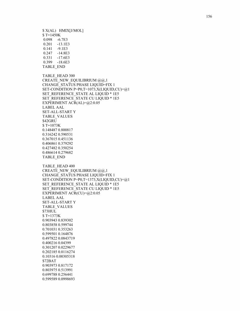
156
$ X(AL) HMIX[J/MOL] $ T=1450K 0.098 -6.7E3 0.201 -13.1E3 0.141 -9.1E3 0.247 -14.8E3 0.331 -17.6E3 0.399 -18.6E3 TABLE_END TABLE_HEAD 300 CREATE_NEW_EQUILIBRIUM @@,1 CHANGE_STATUS PHASE LIQUID=FIX 1 SET-CONDITION P=P0,T=1073,X(LIQUID,CU)=@1 SET_REFERENCE_STATE AL LIQUID * 1E5 SET_REFERENCE_STATE CU LIQUID * 1E5 EXPERIMENT ACR(AL)=@2:0.05 LABEL AAL SET-ALL-START Y TABLE_VALUES $42GRU $ T=1073K 0.148487 0.800817 0.316242 0.590531 0.367015 0.451136 0.406861 0.379292 0.427482 0.350254 0.486614 0.279682 TABLE_END TABLE_HEAD 400 CREATE_NEW_EQUILIBRIUM @@,1 CHANGE_STATUS PHASE LIQUID=FIX 1 SET-CONDITION P=P0,T=1373,X(LIQUID,CU)=@1 SET_REFERENCE_STATE AL LIQUID * 1E5 SET_REFERENCE_STATE CU LIQUID * 1E5 EXPERIMENT ACR(CU)=@2:0.05 LABEL AAL SET-ALL-START Y TABLE_VALUES $73HUL $ T=1373K 0.903943 0.839302 0.803858 0.599744 0.701031 0.353263 0.599501 0.164876 0.497822 0.0843719 0.400216 0.04399 0.301207 0.0229677 0.202185 0.0116274 0.10316 0.00305318 $72BAT 0.903973 0.817172 0.803975 0.513991 0.699788 0.256441 0.599589 0.0998693

157
0.49923 0.0608628 0.400233 0.0315419 0.301215 0.0174353 0.202191 0.00747801 0.103162 0.00167007 TABLE_END TABLE_HEAD 500 CREATE_NEW_EQUILIBRIUM @@,1 CHANGE_STATUS PHASE LIQUID=FIX 1 SET-CONDITION P=P0,T=1373,X(LIQUID,CU)=@1 SET_REFERENCE_STATE AL LIQUID * 1E5 SET_REFERENCE_STATE CU LIQUID * 1E5 EXPERIMENT ACR(AL)=@2:0.05 LABEL AAL SET-ALL-START Y TABLE_VALUES $85WIL $ T=1373K 0.179114 0.788877 0.25216 0.683963 0.327961 0.57629 0.372098 0.487893 0.425874 0.392608 0.468626 0.311123 0.508605 0.246227 0.543069 0.190998 0.620241 0.0860956 0.658808 0.0474755 0.751021 0.0090046 0.85282 0.000989033 0.951857 0.00126451 0.57339 0.146823 0.399697 0.422964 $69MIT 0.0923051 0.899285 0.173661 0.752901 0.292135 0.621834 0.396855 0.489345 0.486555 0.276594 0.573388 0.148206 $73HUL 0.104702 0.886872 0.203867 0.793095 0.30178 0.609412 0.40105 0.439565 0.49895 0.265564 0.599571 0.1137 0.700102 0.0268435 0.80192 0.00499681 0.902339 0.00112677 TABLE_END $ 73Hair 773K TABLE_HEAD 600 CREATE_NEW_EQUILIBRIUM @@,1

158
CHANGE_STATUS PHASE @1=FIX 1 SET-CONDITION P=P0,T=773,X(@1,CU)=@2 SET_REFERENCE_STATE AL FCC * 1E5 SET_REFERENCE_STATE CU FCC * 1E5 EXPERIMENT HMR(@1)=@3:1000 LABEL AHS SET-ALL-START Y TABLE_VALUES FCC 0.93 -6190 FCC 0.86 -9150 GAMMA_D83 0.69 -20290 GAMMA_D83 0.66 -21290 GAMMA_D83 0.637 -21190 ALCU_DELTA 0.60 -20670 ALCU_ZETA 0.55 -20400 ALCU_ETA 0.5001 -19920 ALCU_THETA 0.33 -13050 TABLE_END TABLE_HEAD 700 CREATE_NEW_EQUILIBRIUM @@,1 CHANGE_STATUS PHASE @1=FIX 1 SET-CONDITION P=P0,T=298,X(@1,CU)=@2 SET_REFERENCE_STATE AL FCC * 1E5 SET_REFERENCE_STATE CU FCC * 1E5 EXPERIMENT HMR(@1)=@3:3000 LABEL AHS SET-ALL-START Y TABLE_VALUES $ First-Principles VASP-GGA ALCU_GP 0.25 -9609 ALCU_PRIME 0.3333 -20467 TABLE_END CREATE_NEW_EQUILIBRIUM 800,1 CHANGE_STATUS PHASE ALCU_THETA=FIX 1 SET-CONDITION P=P0,T=298.15,X(ALCU_THETA,CU)=0.333 SET_REFERENCE_STATE AL FCC * 1E5 SET_REFERENCE_STATE CU FCC * 1E5 $Wolverton EXPERIMENT SMR(ALCU_THETA)=-2.079:1 LABEL AHS SET-ALL-START Y CREATE_NEW_EQUILIBRIUM 801,1 CHANGE_STATUS PHASE ALCU_PRIME=FIX 1 SET-CONDITION P=P0,T=298.15,X(ALCU_PRIME,CU)=0.3333 SET_REFERENCE_STATE AL FCC * 1E5 SET_REFERENCE_STATE CU FCC * 1E5 $Wolverton EXPERIMENT SMR(ALCU_PRIME)=-5.155:1 LABEL AHS SET-ALL-START Y TABLE_HEAD 900 CREATE_NEW_EQUILIBRIUM @@,1
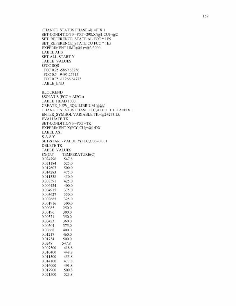
159
CHANGE_STATUS PHASE @1=FIX 1 SET-CONDITION P=P0,T=298,X(@1,CU)=@2 SET_REFERENCE_STATE AL FCC * 1E5 SET_REFERENCE_STATE CU FCC * 1E5 EXPERIMENT HMR(@1)=@3:3000 LABEL AHS SET-ALL-START Y TABLE_VALUES $FCC SQS FCC 0.25 -5869.63256 FCC 0.5 -9495.25715 FCC 0.75 -11266.64772 TABLE_END BLOCKEND $SOLVUS (FCC + Al2Cu) TABLE_HEAD 1000 CREATE_NEW_EQUILIBRIUM @@,1 CHANGE_STATUS PHASE FCC,ALCU_THETA=FIX 1 ENTER_SYMBOL VARIABLE TK=@2+273.15; EVALUATE TK SET-CONDITION P=P0,T=TK EXPERIMENT X(FCC,CU)=@1:DX LABEL AS1 S-A-S Y SET-START-VALUE Y(FCC,CU)=0.001 DELETE TK TABLE_VALUES $X(CU) TEMPERATURE(C) 0.024796 547.8 0.021184 525.0 0.017607 500.0 0.014283 475.0 0.011338 450.0 0.008591 425.0 0.006424 400.0 0.004915 375.0 0.003627 350.0 0.002685 325.0 0.001916 300.0 0.00085 250.0 0.00196 300.0 0.00371 350.0 0.00423 360.0 0.00504 375.0 0.00668 400.0 0.01217 460.0 0.01734 500.0 0.0248 547.8 0.007500 418.8 0.010400 448.8 0.011500 455.8 0.014100 477.8 0.016000 491.8 0.017900 500.8 0.021500 523.8
160
0.022000 524.8 0.016800 499.8 0.013900 474.8 0.006700 399.8 0.002000 299.8 0.004200 353.8 0.006200 398.8 0.011500 449.8 0.017900 499.8 0.019400 513.8 0.022700 530.8 0.023800 539.8 0.012800 460.8 0.017100 489.8 0.020500 515.8 0.023300 531.8 TABLE_END $LIQUIDUS (FCC + LIQUID) TABLE_HEAD 1100 CREATE_NEW_EQUILIBRIUM @@,1 CHANGE_STATUS PHASE FCC,LIQUID=FIX 1 ENTER_SYMBOL VARIABLE TK=@3+273.15; EVALUATE TK SET-CONDITION P=P0,T=TK EXPERIMENT X(LIQUID,CU)=@1:DX,X(FCC,CU)=@2:DX LABEL ALF S-A-S Y SET-START-VALUE Y(LIQUID,CU)=@1 Y(FCC,CU)=@2 DELETE TK TABLE_VALUES $X(LIQUID,CU) X(FCC,CU) TEMPERATURE(C) 0.976800 0.990000 1081.4 0.954000 0.969800 1077.9 0.931900 0.950000 1074.9 0.910800 0.929700 1069.4 0.890000 0.909900 1062.4 0.869000 0.890000 1054.9 0.858900 0.890000 1051.9 0.848800 0.869900 1046.9 0.840000 0.859800 1040.9 0.830000 0.844000 1031.9 0.929700 0.954000 1076.9 0.909900 0.931900 1071.9 0.890000 0.910800 1062.9 0.869900 0.890000 1055.9 0.840000 0.869000 1048.9 0.835000 0.858900 1042.9 0.830000 0.844000 1031.9 $Al-rich side 0.008900 0.001000 655.2 0.050000 0.006400 630.8 0.056000 0.008200 626.8 0.100000 0.012800 599.8 0.139000 0.018600 573.8 0.102000 0.012800 598.8
161
0.131000 0.017100 579.8 0.152000 0.020500 564.8 0.166000 0.023300 554.8 0.026000 0.003300 643.7 0.016800 0.002500 647.8 0.004000 0.000700 656.8 0.166600 0.024000 551.8 0.164400 0.023900 553.3 0.160000 0.023000 557.3 0.008600 0.001550 652.0 0.026000 0.003830 640.0 0.045000 0.005790 630.0 0.096000 0.012200 600.0 0.154000 0.022200 561.0 TABLE_END $LIQUIDUS (THETA + LIQUID) TABLE_HEAD 1200 CREATE_NEW_EQUILIBRIUM @@,1 CHANGE_STATUS PHASE ALCU_THETA,LIQUID=FIX 1 ENTER_SYMBOL VARIABLE TK=@2+273.15; EVALUATE TK SET-CONDITION P=P0,T=TK EXPERIMENT X(LIQUID,CU)=@1:DX LABEL ALT S-A-S Y SET-START-VALUE Y(LIQUID,CU)=0.001 DELETE TK TABLE_VALUES $X(LIQUID,CU) TEMPERATURE(C) 0.220617 566 0.258603 579 0.298048 587 0.31506 589 0.282000 585.8 0.289900 587.8 TABLE_END $LIQUIDUS (ETA + LIQUID) TABLE_HEAD 1250 CREATE_NEW_EQUILIBRIUM @@,1 CHANGE_STATUS PHASE ALCU_ETA,LIQUID=FIX 1 ENTER_SYMBOL VARIABLE TK=@3+273.15; EVALUATE TK SET-CONDITION P=P0,T=TK EXPERIMENT X(LIQUID,CU)=@1:DX LABEL ALET S-A-S Y SET-START-VALUE Y(LIQUID,CU)=0.001,Y(ALCU_ETA,CU)=0.01 DELETE TK TABLE_VALUES $X(LIQUID,CU) X(ALCU_ETA,CU) TEMPERATURE(C) $33Sto 0.359900 0.5 620.8 0.350900 0.5 607.8 0.342000 0.5 597.8

162
$00Unk 0.322000 0.5 590.8 0.331000 0.5 591.8 0.335000 0.5 595.8 0.339800 0.5 600.8 0.348900 0.5 608.8 0.357900 0.5 619.8 0.363000 0.5 623.8 TABLE_END $ Eutectic: LIQUID = FCC(AL) + AL2CU T=548.2C CREATE_NEW_EQUILIBRIUM 1301,1 CHANGE_STATUS PHASE LIQUID,FCC,ALCU_THETA=FIX 1 SET-CONDITION P=P0 EXPERIMENT T=821.35:DT EXPERIMENT X(FCC,CU)=0.0248:DX,X(LIQUID,CU)=0.171:DX EXPERIMENT X(ALCU_THETA,CU)=0.319:DX LABEL APE SET-ALL-START 821.35 Y SET-START-VALUE T=821.35 Y(LIQUID,CU)=0.171 Y(FCC,CU)=0.0248 $ Peritectic: LIQUID + Eta = AL2CU T=591C CREATE_NEW_EQUILIBRIUM 1302,1 CHANGE_STATUS PHASE LIQUID,ALCU_ETA,ALCU_THETA=FIX 1 SET-CONDITION P=P0 EXPERIMENT T=864.15:DT EXPERIMENT X(LIQUID,CU)=0.322:DX,X(ALCU_THETA,CU)=0.328:DX EXPERIMENT X(ALCU_ETA,CU)=0.498:DX LABEL APE SET-ALL-START 864.15 Y SET-START-VALUE T=864.15 Y(LIQUID,CU)=0.322 Y(ALCU_ETA,CU)=0.01 $ Peritectic: LIQUID + Epsilon = Eta T=624C CREATE_NEW_EQUILIBRIUM 1303,1 CHANGE_STATUS PHASE LIQUID,ALCU_ETA,ALCU_EPSILON=FIX 1 SET-CONDITION P=P0 EXPERIMENT T=897.15:DT EXPERIMENT X(LIQUID,CU)=0.363:DX,X(ALCU_EPSILON,CU)=0.55:DX EXPERIMENT X(ALCU_ETA,CU)=0.518:DX LABEL APE SET-ALL-START 897.15 Y SET-START-VALUE T=897.15 Y(LIQUID,CU)=0.363 Y(ALCU_EPSILON,CU)=0.1 SET-START-VALUE Y(ALCU_ETA,CU)=0.01 $ eutectoid: epsilon=Eta +delta T<580C CREATE_NEW_EQUILIBRIUM 1304,1 CHANGE_STATUS PHASE ALCU_EPSILON,ALCU_ETA,ALCU_DELTA=FIX 1 SET-CONDITION P=P0 EXPERIMENT T<853:1 LABEL APE SET-ALL-START 853 Y SET-START-VALUE T=853 Y(ALCU_EPSILON,CU)=0.1 Y(ALCU_ETA,CU)=0.01 $ Congruent ZETA = EPSILON 590C CREATE_NEW_EQUILIBRIUM 1305,1 CHANGE_STATUS PHASE ALCU_ZETA,ALCU_EPSILON=FIX 1
163
SET-CONDITION P=P0,X(ALCU_ZETA,CU)-X(ALCU_EPSILON,CU)=0 EXPERIMENT T=863:DT $EXPERIMENT X(ALCU_ZETA,CU)=0.55:DX LABEL APE SET-ALL-START 863.15 Y SET-START-VALUE T=863.15 Y(ALCU_EPSILON,CU)=0.1 $ Peritectic: LIQUID + GAMMA_H = EPSILON T=958C CREATE_NEW_EQUILIBRIUM 1306,1 CHANGE_STATUS PHASE LIQUID,ALCU_EPSILON,GAMMA_H=FIX 1 SET-CONDITION P=P0 EXPERIMENT T=1231.15:DT EXPERIMENT X(LIQUID,CU)=0.598:DX,X(ALCU_EPSILON,CU)=0.621:DX $EXPERIMENT X(GAMMA_H,CU)=0.629:DX LABEL APE SET-ALL-START 1231.15 Y SET-START-VALUE T=1231.15 Y(LIQUID,CU)=0.598 Y(ALCU_EPSILON,CU)=0.24 SET-START-VALUE Y(GAMMA_H,CU)=0.1 $ Peritectoid: Epsilon + GAMMA_D83 = Delta T=686C CREATE_NEW_EQUILIBRIUM 1307,1 CHANGE_STATUS PHASE ALCU_DELTA,ALCU_EPSILON,GAMMA_D83=FIX 1 SET-CONDITION P=P0 EXPERIMENT T=959.15:DT EXPERIMENT X(ALCU_EPSILON,CU)=0.592:DX EXPERIMENT X(GAMMA_D83,CU)=0.628:DX $EXPERIMENT X(ALCU_DELTA,CU)=0.619:DX LABEL APE SET-ALL-START 959.15 Y SET-START-VALUE T=959.15 Y(GAMMA_D83,CU)=0.1 SET-START-VALUE Y(ALCU_EPSILON,CU)=0.2 $ Congruent Melting: BCC_A2 = LIQUID T=1049C CREATE_NEW_EQUILIBRIUM 1308,1 CHANGE_STATUS PHASE LIQUID,BCC_A2=FIX 1 SET-CONDITION P=P0,X(LIQUID,CU)-X(BCC_A2,CU)=0 EXPERIMENT T=1322.15:DT EXPERIMENT X(BCC_A2,CU)=0.75:DX LABEL APE SET-ALL-START 1322.15 Y SET-START-VALUE T=1322.15 Y(LIQUID,CU)=0.9 Y(BCC_A2,CU)=0.9 $ Eutectoid: BCC_A2 = FCC(CU) + GAMMA_D83 T=567C CREATE_NEW_EQUILIBRIUM 1309,1 CHANGE_STATUS PHASE BCC_A2,FCC,GAMMA_D83=FIX 1 SET-CONDITION P=P0 EXPERIMENT T=840.15:DT EXPERIMENT X(FCC,CU)=0.803:DX,X(GAMMA_D83,CU)=0.69:DX EXPERIMENT X(BCC_A2,CU)=0.761:DX LABEL APE SET-ALL-START 840.15 Y SET-START-VALUE T=840.15 Y(BCC_A2,CU)=0.761 Y(FCC,CU)=0.803 $ Eutectic: LIQUID = FCC(CU) + BCC_A2 T=1032C CREATE_NEW_EQUILIBRIUM 1310,1 CHANGE_STATUS PHASE LIQUID,BCC_A2,FCC=FIX 1

164
SET-CONDITION P=P0 EXPERIMENT T=1305.15:DT EXPERIMENT X(FCC,CU)=0.842:DX,X(LIQUID,CU)=0.83:DX EXPERIMENT X(BCC_A2,CU)=0.82:DX LABEL APE SET-ALL-START 1305.15 Y SET-START-VALUE Y(FCC,CU)=0.842 Y(LIQUID,CU)=0.83 Y(BCC_A2,CU)=0.82 $SOLVUS (FCC + THETA PRIME) TABLE_HEAD 1400 CREATE_NEW_EQUILIBRIUM @@,1 CHANGE_STATUS PHASE FCC,ALCU_PRIME=FIX 1 E-SYM VARIA TK=@2+273.15; EVALUATE TK SET-CONDITION P=P0,T=TK EXPERIMENT X(FCC,CU)=@1:DX LABEL AS2 S-A-S Y SET-START-VALUE Y(FCC,CU)=@1 DELETE TK TABLE_VALUES $73Hor 0.00436468 249.146 0.00650315 314.84 0.00876826 344.716 0.013285 383.415 0.0176503 402.749 TABLE_END $SOLVUS (FCC + Al3Cu) TABLE_HEAD 1500 CREATE_NEW_EQUILIBRIUM @@,1 CHANGE_STATUS PHASE FCC,ALCU_GP=FIX 1 E-SYM VARIA TK=@2+273.15; EVALUATE TK SET-CONDITION P=P0,T=TK EXPERIMENT X(FCC,CU)=@1:DX LABEL AS3 S-A-S Y SET-START-VALUE Y(FCC,CU)=@1 DELETE TK TABLE_VALUES $57Beton high 0.0126178 221.333 0.0198549 245.333 0.0229135 249.333 $73Sat high 0.00690479 178.667 0.00690275 170.667 0.0149331 226.667 0.0149727 220 TABLE_END TABLE_HEAD 1600 CREATE_NEW_EQUILIBRIUM @@,1 CHANGE_STATUS PHASE LIQUID,GAMMA_H=FIX 1

165
E-SYM VARIA TK=@2+273.15; EVALUATE TK SET-CONDITION P=P0,X(LIQUID,AL)=@1 EXPERIMENT T=TK:DT LABEL AGA SET-ALL-START @2 Y SET-START-VALUE Y(LIQUID,AL)=@1,Y(GAMMA_H,AL)=0.5 DELETE TK TABLE_VALUES $ 98Liu 0.34 1025 0.37 980 TABLE_END TABLE_HEAD 1700 CREATE_NEW_EQUILIBRIUM @@,1 CHANGE_STATUS PHASE LIQUID,GAMMA_H=FIX 1 E-SYM VARIA TK=@2+273.15; EVALUATE TK SET-CONDITION P=P0,X(GAMMA_H,AL)=@1 EXPERIMENT T=TK:DT LABEL AGA SET-ALL-START @2 Y SET-START-VALUE Y(LIQUID,AL)=0.4,Y(GAMMA_H,AL)=@1 DELETE TK TABLE_VALUES $98Liu 0.34 991 0.37 962.4 TABLE_END $ SOLIDUS (FCC + BCC) TABLE_HEAD 1800 CREATE_NEW_EQUILIBRIUM @@,1 CHANGE_STATUS PHASE FCC,BCC_A2=FIX 1 E-SYM VARIA TK=@3+273.15; EVALUATE TK SET-CONDITION P=P0,T=TK EXPERIMENT X(FCC,CU)=@1:DX,X(BCC_A2,CU)=@2:DX LABEL AFB S-A-S Y SET-START-VALUE Y(FCC,CU)=@1 Y(BCC_A2,CU)=@2 DELETE TK TABLE_VALUES $X(FCC,CU) X(BCC,CU) TEMPERATURE(C) $72Lin 0.8075 0.7712 650.0 0.8120 0.7761 700.0 0.8146 0.7810 747.0 0.8237 0.7859 800.0 0.8281 0.7931 850.0 0.8329 0.8003 900.0 0.8337 0.8051 925.0 0.8364 0.8070 950.0 0.8402 0.8109 975.0 0.8402 0.8150 1000.0
166
0.8439 0.8195 1023.0 0.8030 0.7608 572.0 0.8040 0.7651 598.0 TABLE_END TABLE_HEAD 1900 CREATE_NEW_EQUILIBRIUM @@,1 CHANGE_STATUS PHASE LIQUID,BCC_A2=FIX 1 E-SYM VARIA TK=@3+273.15; EVALUATE TK SET-CONDITION P=P0,X(BCC_A2,CU)=@2 EXPERIMENT X(LIQUID,CU)=@1:DX,T=TK:DT LABEL ALB $SET-ALL-START TK Y SET-ALL-START @3 Y SET-START-VALUE Y(LIQUID,CU)=@1 Y(BCC_A2,CU)=@2 DELETE TK TABLE_VALUES $33Sto Phase boundary of liquid + bcc 0.830000 0.814000 1036.0 0.820000 0.807000 1040.0 0.808000 0.798000 1044.0 0.792000 0.785000 1048.0 0.765000 0.765000 1050.0 0.737000 0.744000 1048.0 0.720000 0.732000 1048.0 0.708000 0.723000 1040.0 TABLE_END $ SOLIDUS (FCC + BCC) TABLE_HEAD 2000 CREATE_NEW_EQUILIBRIUM @@,1 CHANGE_STATUS PHASE FCC,BCC_A2=FIX 1 E-SYM VARIA TK=@3+273.15; EVALUATE TK SET-CONDITION P=P0,T=TK EXPERIMENT X(FCC,AL)=@1:DX,X(BCC_A2,AL)=@2:DX LABEL AFB S-A-S Y SET-START-VALUE Y(FCC,AL)=@1 Y(BCC_A2,AL)=@2 DELETE TK TABLE_VALUES $X(FCC,AL) X(BCC,AL) TEMPERATURE(C) $98Liu 0.171 0.195 900 0.174 0.208 850 0.175 0.210 800 0.180 0.215 780 0.189 0.225 700 0.198 0.232 600 TABLE_END TABLE_HEAD 2100 CREATE_NEW_EQUILIBRIUM @@,1 CHANGE_STATUS PHASE LIQUID,BCC_A2=FIX 1 E-SYM VARIA TK=@2+273.15;

167
EVALUATE TK SET-CONDITION P=P0,X(LIQUID,AL)=@1 EXPERIMENT T=TK:DT LABEL ALB SET-ALL-START @2 Y SET-START-VALUE Y(LIQUID,AL)=@1,Y(BCC_A2,AL)=@1 DELETE TK TABLE_VALUES $98Liu 0.25 1049 0.30 1041 TABLE_END $ FCC+GAMMA_D83 TABLE_HEAD 2200 CREATE_NEW_EQUILIBRIUM @@,1 CHANGE_STATUS PHASE FCC,GAMMA_D83=FIX 1 E-SYM VARIA TK=@3+273.15; EVALUATE TK SET-CONDITION P=P0,T=TK EXPERIMENT X(FCC,AL)=@1:DX,X(GAMMA_D83,AL)=@2:DX LABEL AGA S-A-S Y SET-START-VALUE Y(FCC,AL)=0.2 Y(GAMMA_D83,AL)=0.01 DELETE TK TABLE_VALUES $X(FCC,AL) X(GAMMA_D83,AL) TEMPERATURE(C) $98Liu 0.202 0.32 500 TABLE_END $ LIQUIDUS (LIQUID + EPSILON) TABLE_HEAD 2300 CREATE_NEW_EQUILIBRIUM @@,1 CHANGE_STATUS PHASE LIQUID,ALCU_EPSILON=FIX 1 E-SYM VARIA TK=@2+273.15; EVALUATE TK SET-CONDITION P=P0,T=TK EXPERIMENT X(LIQUID,CU)=@1:DX LABEL ALE S-A-S Y SET-START-VALUE Y(LIQUID,CU)=0.01 Y(ALCU_EPSILON,CU)=0.2 DELETE TK TABLE_VALUES $X(LIQUID,CU) TEMPERATURE(C) $85Mur 0.39 650.0 0.42 700.0 0.46 750.0 0.49 800.0 0.53 850.0 0.56 900.0 TABLE_END $ LIQUIDUS (LIQUID + EPSILON) TABLE_HEAD 2400
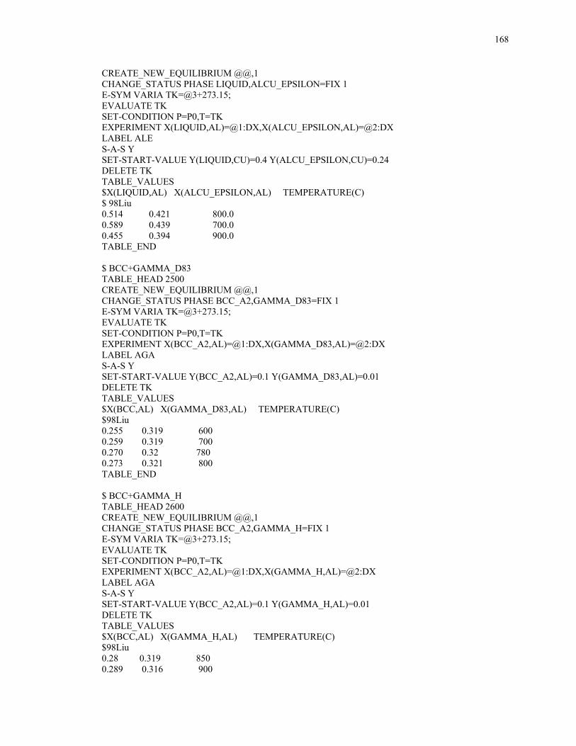
168
CREATE_NEW_EQUILIBRIUM @@,1 CHANGE_STATUS PHASE LIQUID,ALCU_EPSILON=FIX 1 E-SYM VARIA TK=@3+273.15; EVALUATE TK SET-CONDITION P=P0,T=TK EXPERIMENT X(LIQUID,AL)=@1:DX,X(ALCU_EPSILON,AL)=@2:DX LABEL ALE S-A-S Y SET-START-VALUE Y(LIQUID,CU)=0.4 Y(ALCU_EPSILON,CU)=0.24 DELETE TK TABLE_VALUES $X(LIQUID,AL) X(ALCU_EPSILON,AL) TEMPERATURE(C) $ 98Liu 0.514 0.421 800.0 0.589 0.439 700.0 0.455 0.394 900.0 TABLE_END $ BCC+GAMMA_D83 TABLE_HEAD 2500 CREATE_NEW_EQUILIBRIUM @@,1 CHANGE_STATUS PHASE BCC_A2,GAMMA_D83=FIX 1 E-SYM VARIA TK=@3+273.15; EVALUATE TK SET-CONDITION P=P0,T=TK EXPERIMENT X(BCC_A2,AL)=@1:DX,X(GAMMA_D83,AL)=@2:DX LABEL AGA S-A-S Y SET-START-VALUE Y(BCC_A2,AL)=0.1 Y(GAMMA_D83,AL)=0.01 DELETE TK TABLE_VALUES $X(BCC,AL) X(GAMMA_D83,AL) TEMPERATURE(C) $98Liu 0.255 0.319 600 0.259 0.319 700 0.270 0.32 780 0.273 0.321 800 TABLE_END $ BCC+GAMMA_H TABLE_HEAD 2600 CREATE_NEW_EQUILIBRIUM @@,1 CHANGE_STATUS PHASE BCC_A2,GAMMA_H=FIX 1 E-SYM VARIA TK=@3+273.15; EVALUATE TK SET-CONDITION P=P0,T=TK EXPERIMENT X(BCC_A2,AL)=@1:DX,X(GAMMA_H,AL)=@2:DX LABEL AGA S-A-S Y SET-START-VALUE Y(BCC_A2,AL)=0.1 Y(GAMMA_H,AL)=0.01 DELETE TK TABLE_VALUES $X(BCC,AL) X(GAMMA_H,AL) TEMPERATURE(C) $98Liu 0.28 0.319 850 0.289 0.316 900

169
0.303 0.314 1000 TABLE_END $ GAMMA_D83+EPSILON TABLE_HEAD 2700 CREATE_NEW_EQUILIBRIUM @@,1 CHANGE_STATUS PHASE ALCU_EPSILON,GAMMA_D83=FIX 1 E-SYM VARIA TK=@3+273.15; EVALUATE TK SET-CONDITION P=P0,T=TK EXPERIMENT X(ALCU_EPSILON,AL)=@1:DX EXPERIMENT X(GAMMA_D83,AL)=@2:DX LABEL AGA S-A-S Y SET-START-VALUE Y(ALCU_EPSILON,al)=0.75 Y(GAMMA_D83,AL)=0.9 DELETE TK TABLE_VALUES $X(EPSILON,AL) X(GAMMA_D83,AL) TEMPERATURE(C) $98Liu 0.395 0.377 800 0.408 0.384 700 TABLE_END $ GAMMA_H+EPSILON TABLE_HEAD 2800 CREATE_NEW_EQUILIBRIUM @@,1 CHANGE_STATUS PHASE ALCU_EPSILON,GAMMA_H=FIX 1 E-SYM VARIA TK=@3+273.15; EVALUATE TK SET-CONDITION P=P0,T=TK EXPERIMENT X(ALCU_EPSILON,AL)=@1:DX $EXPERIMENT X(GAMMA_H,AL)=@2:DX LABEL AGA S-A-S Y SET-START-VALUE Y(ALCU_EPSILON,CU)=0.24 Y(GAMMA_H,AL)=0.9 DELETE TK TABLE_VALUES $X(EPSILON,AL) X(GAMMA_H,AL) TEMPERATURE(C) $98Liu 0.386 0.374 900 TABLE_END SAVE_WORKSPACES

170
APPENDIX C. THERMO-CALC DATABASE FILE FOR AL-CU SYSTEM
ELEMENT VA VACUUM 0.0000E+00 0.0000E+00 0.0000E+00! ELEMENT AL FCC_A1 2.6982E+01 4.5773E+03 2.8322E+01! ELEMENT CU FCC_A1 6.3546E+01 5.0041E+03 3.3150E+01! FUNCTION GHSERAL 298.15 -7976.15+137.071542*T-24.3671976*T*LN(T) -.001884662*T**2-8.77664E-07*T**3+74092*T**(-1); 7.00000E+02 Y -11276.24+223.02695*T-38.5844296*T*LN(T)+.018531982*T**2 -5.764227E-06*T**3+74092*T**(-1); 9.33600E+02 Y -11277.683+188.661987*T-31.748192*T*LN(T)-1.234264E+28*T**(-9); 2.90000E+03 N ! FUNCTION GHSERCU 298.15 -7770.458+130.485403*T-24.112392*T*LN(T) -.00265684*T**2+1.29223E-07*T**3+52478*T**(-1); 1.35802E+03 Y -13542.33+183.804197*T-31.38*T*LN(T)+3.64643E+29*T**(-9); 3.20000E+03 N ! FUNCTION GCUBCC 298.15 +4017-1.255*T+GHSERCU#; 6000 N ! FUNCTION GALBCC 298.15 +10083-4.813*T+GHSERAL#; 6000 N ! TYPE_DEFINITION % SEQ *! DEFINE_SYSTEM_DEFAULT SPECIE 2 ! DEFAULT_COMMAND DEF_SYS_ELEMENT VA ! PHASE LIQUID:L % 1 1.0 ! CONSTITUENT LIQUID:L :AL,CU : ! PARAMETER G(LIQUID,AL;0) 298.15 +11005.553-11.840873*T +7.9401E-20*T**7+GHSERAL#; 9.33600E+02 Y +10481.974-11.252014*T+1.234264E+28*T**(-9)+GHSERAL#; 2.90000E+03 N ! PARAMETER G(LIQUID,CU;0) 298.15 +12964.84-9.510243*T -5.83932E-21*T**7+GHSERCU#; 1.35802E+03 Y +13495.4-9.920463*T-3.64643E+29*T**(-9)+GHSERCU#; 3.20000E+03 N ! PARAMETER G(LIQUID,AL,CU;0) 298.15 -66054+8.363*T; 6000 N ! PARAMETER G(LIQUID,AL,CU;1) 298.15 32489-8.524*T; 6000 N ! PARAMETER G(LIQUID,AL,CU;2) 298.15 7420-10.702*T; 6000 N ! TYPE_DEFINITION ( GES A_P_D FCC_A1 MAGNETIC -3.0 2.80000E-01 ! PHASE FCC_A1 %( 2 1 1 ! CONSTITUENT FCC_A1 :AL%,CU% : VA% : ! PARAMETER G(FCC_A1,AL:VA;0) 298.15 +GHSERAL#; 6000 N ! PARAMETER G(FCC_A1,CU:VA;0) 298.15 +GHSERCU#; 6000 N ! PARAMETER G(FCC_A1,AL,CU:VA;0) 298.15 -43205-4.630*T; 6000 N ! PARAMETER G(FCC_A1,AL,CU:VA;1) 298.15 45224-6.789*T; 6000 N ! PARAMETER G(FCC_A1,AL,CU:VA;2) 298.15 -16747+11.614*T; 6000 N ! PHASE ALCU_THETA % 2 0.6667 0.3333 ! CONSTITUENT ALCU_THETA :AL : AL,CU : ! PARAMETER G(ALCU_THETA,AL:AL;0) 298.15 +GALBCC#; 6000 N ! PARAMETER G(ALCU_THETA,AL:CU;0) 298.15 -16025+2.719*T +0.6667*GHSERAL#+0.3333*GHSERCU#; 6000 N ! PHASE ALCU_PRIME % 2 0.6667 0.3333 !

171
CONSTITUENT ALCU_PRIME :AL : CU : ! PARAMETER G(ALCU_PRIME,AL:CU;0) 298.15 -16783+5.434*T +0.6667*GHSERAL#+0.3333*GHSERCU#; 6000 N ! PHASE ALCU_GP % 2 .75 .25 ! CONSTITUENT ALCU_GP :AL: CU : ! PARAMETER G(ALCU_GP,AL:CU;0) 298.15 -8389+0.385*T +.75*GHSERAL#+.25*GHSERCU#; 6000 N ! TYPE_DEFINITION & GES A_P_D BCC_A2 MAGNETIC -1.0 4.00000E-01 ! PHASE BCC_A2 %& 2 1 3 ! CONSTITUENT BCC_A2 :AL,CU : VA% : ! PARAMETER G(BCC_A2,AL:VA;0) 298.15 +GALBCC#; 2.90000E+03 N ! PARAMETER G(BCC_A2,CU:VA;0) 298.15 +GCUBCC#; 3.20000E+03 N ! PARAMETER G(BCC_A2,AL,CU:VA;0) 298.15 -73083+4.810*T; 6000 N ! PARAMETER G(BCC_A2,AL,CU:VA;1) 298.15 48345-7.216*T; 6000 N ! PHASE ALCU_EPSILON % 2 .5 .5 ! CONSTITUENT ALCU_EPSILON :AL,CU : CU : ! PARAMETER G(ALCU_EPSILON,AL:CU;0) 298.15 -20313+3.000*T +.5*GHSERAL#+.5*GHSERCU#; 6000 N ! PARAMETER G(ALCU_EPSILON,CU:CU;0) 298.15 22019+GHSERCU#; 6000 N ! PARAMETER G(ALCU_EPSILON,AL,CU:CU;0) 298.15 -29635-27.517*T; 6000 N ! PHASE ALCU_ETA % 2 .5 .5 ! CONSTITUENT ALCU_ETA :AL,CU : CU : ! PARAMETER G(ALCU_ETA,AL:CU;0) 298.15 -20315+2.079*T +.5*GHSERAL#+.5*GHSERCU#; 6000 N ! PARAMETER G(ALCU_ETA,CU:CU;0) 298.15 +GCUBCC#; 6000 N ! PARAMETER G(ALCU_ETA,AL,CU:CU;0) 298.15 -17953; 6000 N ! PHASE ALCU_DELTA % 2 .4 .6 ! CONSTITUENT ALCU_DELTA :AL : CU : ! PARAMETER G(ALCU_DELTA,AL:CU;0) 298.15 -22278+1.702*T +.4*GHSERAL#+.6*GHSERCU#; 6000 N ! PHASE ALCU_ZETA % 2 .45 .55 ! CONSTITUENT ALCU_ZETA :AL : CU : ! PARAMETER G(ALCU_ZETA,AL:CU;0) 298.15 -21384+1.960*T +.45*GHSERAL#+.55*GHSERCU#; 6000 N ! PHASE GAMMA_D83 % 3 .3077 .0769 .6154 ! CONSTITUENT GAMMA_D83 :AL : AL,CU : CU : ! PARAMETER G(GAMMA_D83,AL:AL:CU;0) 298.15 -24185+31*T-4*T*LN(T) +.3846*GHSERAL#+.6154*GHSERCU#; 6000 N ! PARAMETER G(GAMMA_D83,AL:CU:CU;0) 298.15 -20622+28.5*T-4*T*LN(T) +.3077*GHSERAL#+.6923*GHSERCU#; 6000 N !

172
PHASE GAMMA_H % 3 .3077 .0769 .6154 ! CONSTITUENT GAMMA_H :AL : AL,CU : CU : ! PARAMETER G(GAMMA_H,AL:AL:CU;0) 298.15 -16339-4*T+.3846*GHSERAL# +.6154*GHSERCU#; 6000 N ! PARAMETER G(GAMMA_H,AL:CU:CU;0) 298.15 -15185-4.5*T+.3077*GHSERAL# +.6923*GHSERCU#; 6000 N !
173
REFERENCES
1. A. Guinier, Nature, 142 (1938) 569.
2. G. D. Preston, Proc. Roy. Soc. A, 167 (1938) 526-538.
3. C. Wolverton, Philos. Mag. Lett., 79 (1999) 683-690.
4. J. J. Pepe and W. F. Savage, Welding Journal, 46 (1967) 411-422.
5. D. B. Miracle, Acta Mater, 41 (1993) 649-684.
6. M. Kogachia, T. Haraguchia and S. M. Kim, Intermetallics, 6 (1998) 499-510.
7. J. L. Jordan and S. C. Deevi, Intermetallics, 11 (2003) 507-528.
8. A. J. Bradley and A. Taylor, Proc. R. Soc. London, Ser. A, 159 (1937) 56.
9. H. Xiao and I. Baker, Acta Mater, 43 (1995) 391-396.
10. I. Baker, Mater. Sci. Eng. A, 193 (1995) 1-13.
11. Y. Mishin, A. Y. Lozovoi and A. Alavi, Phys. Rev. B, 67 (2003) 014201.
12. M. Fähnle, B. Meyer and G. Bester, Intermetallics, 7 (1999) 1307-1308.
13. L. Kaufman and H. Bernstein, Computer Calculation of Phase Diagrams
(Academic Press, New York, 1970).
14. B. Sundman, B. Jansson and J.-O. Andersson, CALPHAD, 9 (1985) 153-190.
15. J.-O. Andersson, T. Helander, L. Hoglund, P. Shi and B. Sundman, Calphad, 26
(2002) 273-312.
16. W. Kohn and L. Sham, Phys. Rev. A, 140 (1965) 1133.
17. C. Wolverton and A. Zunger, Phys. Rev. Lett., 75 (1995) 3162-3165.
18. A. Zunger, L. G. Wang, G. L. W. Hart and M. Sanati, Model. Simul. Mater. Sc.,
10 (2002) 685-706.

174
19. A. van de Walle and M. Asta, Model. Simul. Mater. Sc., 10 (2002) 521-538.
20. A. van de Walle and G. Ceder, Journal of Phase Equilibria (USA), 23 (2002) 348-
359.
21. C. Wolverton and V. Ozolins, Phys. Rev. Lett., 86 (2001) 5518-5521.
22. S. Baroni, P. Giannozzi and A. Testa, Phys. Rev. Lett., 58 (1987) 1861.
23. I. Ansara, A. T. Dinsdale and M. H. Rand, Eds., COST 507: Thermochemical
Database for Light Metal Alloys, vol. 2 (European Commission, 1998).
24. C. Wolverton, X. Y. Yan, R. Vijayaraghavan and V. Ozolins, Acta Mater., 50
(2002) 2187-2197.
25. D. A. Porter and K. E. Easterling, Phase transformations in metals and alloys.
26. R. H. Beton and E. C. Rollason, Journal of the Institute of Metals, 86 (1957-58)
77-85.
27. K. G. Satyanarayana, K. Jayapalan and T. R. Anantharaman, Current Science, 41
(1973) 6-9.
28. A. T. Dinsdale, CALPHAD, 15 (1991) 317-425.
29. O. Redlich and A. T. Kister, Ind. Eng. Chem., 40 (1948) 345-348.
30. M. Hillert and L. Staffansson, Acta Chem. Scand., 24 (1970) 3618-3626.
31. D. M. Ceperley and B. J. Alder, Phys. Rev. Lett., 45 (1980) 566.
32. J. P. Perdew and A. Zunger, Phys. Rev. B, 23 (1981) 5048.
33. J. W. D. Connolly and A. R. Williams, Phys. Rev. B, 27 (1983) 5169-5172.
34. A. Zunger, S. H. Wei, L. G. Ferreira and J. E. Bernard, Phys. Rev. Lett., 65 (1990)
353-356.

175
35. S. H. Wei, L. G. Ferreira, J. E. Bernard and A. Zunger, Phys. Rev. B, 42 (1990)
9622-9649.
36. B. L. Gyorffy, Phys. Rev. B, 5 (1972) 2382-2384.
37. Z. W. Lu, S. H. Wei and A. Zunger, Phys. Rev. B, 44 (1991) 3387-3390.
38. Z. W. Lu, S. H. Wei and A. Zunger, Phys. Rev. B, 45 (1992) 10314-10330.
39. A. V. Ruban, S. I. Simak, S. Shallcross and H. L. Skriver, Phys. Rev. B, 67 (2003)
214302.
40. J. C. Mikkelsen and J. B. Boyce, Phys. Rev. Lett., 49 (1982) 1412-1415.
41. K. C. Hass, L. C. Davis and A. Zunger, Phys. Rev. B, 42 (1990) 3757-3760.
42. V. Ozolins, C. Wolverton and A. Zunger, Phys. Rev. B, 57 (1998) 6427-6443.
43. C. Wolverton, Acta Mater, 49 (2001) 3129-3142.
44. A. van de Walle, M. Asta and G. Ceder, Calphad, 26 (2003) 539-553.
45. H. T. Stokes and D. M. Hatch, www.physics.byu.edu/~stokesh/isotropy.html,
FINDSYM, www.physics.byu.edu/~stokesh/isotropy.html (2001),
46. D. Vanderbilt, Phys. Rev. B, 41 (1990) 7892-7895.
47. G. Kresse and J. Hafner, J. Phys.-Condes. Matter, 6 (1994) 8245-8257.
48. G. Kresse and J. Furthmuller, Phys. Rev. B, 54 (1996) 11169-11186.
49. G. Kresse and J. Furthmuller, Comput. Mater. Sci., 6 (1996) 15-50.
50. J. P. Perdew, J. A. Chevary, S. H. Vosko, K. A. Jackson, M. R. Pederson, D. J.
Singh and C. Fiolhais, Phys. Rev. B, 46 (1992) 6671-6687.
51. C. Amador, W. R. L. Lambrecht and B. Segall, Phys. Rev. B, 46 (1992) 1870.
52. H. J. Monkhorst and J. D. Pack, Phys. Rev. B, 13 (1972) 5188.
53. P. G. Evans, E. D. Isaacs, G. Aeppli, Z. Cai and B. Lai, Science, 295 (2002) 1042.

176
54. N. Kimura and Y. Kakehashi, J. Magn. Magn. Mater., 226-230 (2001) 1019-
1020.
55. E. Fawcett, H. L. Alberts, V. Y. Galkin, D. R. Noakes and J. V. Yakhmi, Rev.
Mod. Phys., 66 (1994) 25.
56. S. C. Singhal and W. L. Worrell, Metall. Trans., 4 (1973) 1125-1128.
57. H. J. Goldschmidt and J. A. Brand, J. Less-Common Met., 3 (1961) 44.
58. J. A. Catterall and S. M. Barker, Plansee Proc., (1964) 577.
59. C. Sigli, M. Kosugi and J. M. Sanchez, Phys. Rev. Lett., 57 (1986) 253-256.
60. S. C. Singhal and W. L. Worrell, Metall. Trans., 4 (1973) 895-898.
61. R. Krishnan, S. P. Garg and N. Krishnamurthy, J. Alloy Phase Diagrams, 3
(1987) 1.
62. P. E. A. Turchi, A. Gonis, V. Drchal and J. Kudrnovsky, Phys. Rev. B, 64 (2001)
085112.
63. N. K. Arkhipova, S. M. Klotsman, I. P. Polikarpova, G. N. Tatarinova, A. N.
Timofeev and L. M. Veretennikov, Phys. Rev. B, 30 (1984) 1788-1796.
64. V. P. Itkin, in Phase diagrams of binary iron alloys H. Okamoto, Ed. (ASM
International, Materials Park, OH, 1993) pp. 102-129.
65. G. D. Preston, Philos. Mag., 13 (1932) 419-425.
66. A. T. Aldred, Phys. Rev. B, 14 (1976) 219-227.
67. Y. A. Dorofeyev, A. Z. Menshikov and G. A. Takzey, Phys. Met. Metallogr., 55
(1983) 102-109.
68. N. I. Kulikov and C. Demangeat, Phys. Rev. B, 55 (1997) 3533-3542.
69. W. A. Dench, Trans. Faraday Soc., 59 (1962) 1279.

177
70. H. Akai and P. H. Dederichs, Phys. Rev. B, 47 (1993) 8739-8747.
71. P. Olsson, I. A. Abrikosov, L. Vitos and J. Wallenius, J. Nuclear Mat., 321 (2003)
84-90.
72. P. J. Craievich, M. Weinert, J. M. Sanchez and R. E. Watson, Physical Review
Letters, 72 (1994) 3076-3079.
73. M. Sob, L. G. Wang and V. Vitek, Computational Materials Science, 8 (1997)
100-106.
74. L. G. Wang, M. Sob and Z. Y. Zhang, Journal of Physics and Chemistry of
Solids, 64 (2003) 863-872.
75. S. Muller, L. W. Wang, A. Zunger and C. Wolverton, Phys. Rev. B, 60 (1999)
16448-16462.
76. J. Hair and D. B. Downie, Faraday Symp. Chem. Soc., 8 (1973) 56-63.
77. W. Oelsen and W. Middel, Mitt. Kaiser Wilhelm Inst. Eisenforsch. (Dusseldrof),
19 (1937) 1-26.
78. J. L. Murray, Int. Met. Rev., 30 (1985) 211-233.
79. X. J. Liu, I. Ohnuma, R. Kainuma and K. Ishida, J. Alloy. Compd., 264 (1998)
201-208.
80. U. K. Stolz, I. Arpshofen, F. Sommer and B. Predel, J. Phase Equilibria, 14
(1993) 473-478.
81. V. Witusiewicz, U. K. Stolz, I. Arpshofen and F. Sommer, Z. Metallkd., 89 (1998)
704-713.
82. D. S. Kanibolotsky, O. A. Bieloborodova, N. V. Kotova and V. V. Lisnyak,
Journal of thermal analysis and calorimetry, 70 (2002) 975-983.

178
83. B. Jansson, Trita-Mac-0234 (Royal Institute of Technology, Stockholm, Sweden,
1984).
84. Y. Wang, S. Curtarolo, C. Jiang, R. Arroyave, T. Wang, G. Ceder, L. Q. Chen and
Z. K. Liu, CALPHAD, (2004) in press.
85. R. Hultgren, P. D. Desai, D. T. Hawkins, M. Gleiser and K. K. Kelley, Selected
Value of the Thermodynamic Properties of Binary Alloys (ASM, Metal Park, OH,
1973).
86. G. Grube and P. Hantelmann, Z. Elektrochem., 48 (1942) 90.
87. R. Hultgren, R. L. Orr and K. K. Kelley, Supplement to Selected Value of the
Thermodynamic Properties of Binary Alloys (ASM, Metal Park, OH, 1973).
88. G. I. Batalin, E. A. Beloborodova and V. N. Vasilev, Ukr. Khim. Zh., 38 (1972)
920-923.
89. T. C. Wilder, Trans. Metall. Soc. AIME, 233 (1965) 1202.
90. H. Mitani and H. Nagai, J. Jpn. Inst. Met., 33 (1969) 344.
91. H. Hori and K. Hirano, J. Jpn. Inst. Met., 37 (1973) 142-148.
92. G. Borelius, J. Anderson and K. Gullberg, Ing. Vetenskaps Akad. Handl., 169
(1943) 5-37.
93. O. Reiso, H. G. Overlie and N. Ryum, Metall. Trans. A, 21A (1990) 1689-1695.
94. A. L. Wilson, PhD Dissertation, The Pennsylvania State University (2001).
95. K. Chattopadhyay, V. T. Swamy and S. L. Agrwala, Acta Materialia, 38 (1990)
521-531.
96. W. T. Kim and B. Cantor, Acta Materialia, 42 (1994) 3045-3053.
97. M. G. Hall and C. W. Haworth, Acta Materialia, 18 (1970) 331-337.

179
98. J. R. Frade and M. Cable, J. Am. Ceram. Soc., 77 (1994) 999-1004.
99. B. P. Burton, J. E. Osburn and A. Pasturel, Phys. Rev. B, 45 (1992) 7677-7683.
100. P. A. Korzhavyi, A. V. Ruban, A. Y. Lozovoi, Y. K. Vekilov, I. A. Abrikosov and
B. Johansson, Phys. Rev. B, 61 (2000) 6003-6018.
101. L. M. Pike, Y. A. Chang and C. T. Liu, Acta Mater, 45 (1997) 3709-3719.
102. C. L. Fu, Y. Y. Ye, M. H. Yoo and K. M. Ho, Phys. Rev. B, 48 (1993) 6712.
103. B. Meyer and M. Fahnle, Phys. Rev. B, 59 (1999) 6072.
104. A. Alavi, A. Y. Lozovoi and M. W. Finnis, Phys. Rev. Lett., 83 (1999) 979.
105. C. Wagner and W. Schottky, Z. Physik. Chem. B, 11 (1930) 163.
106. P. E. Blöchl, Phys. Rev. B, 50 (1994) 17953.
107. G. Kresse and J. Joubert, Phys. Rev. B, 59 (1999) 1758.
108. M. J. Mehl, J. E. Osburn, D. A. Papaconstantopoulos and B. M. Klein, Phys. Rev.
B, 41 (1990) 10311-10323.
109. F. Birch, J. Geophys. Res., 83 (1978) 1257.
110. P. Nash and O. Kleppa, Journal of Alloys and Compounds, 321 (2001) 228-231.
111. B. Bai and G. S. Collins, in High-Temperature Ordered Intermetallic Alloys VIII,
MRS Symposia Proceedings No. 552 M. J. Mills, Ed. (Materials Research Society,
Pittsburgh, 1999) pp. KK8.7.1-6.
112. K. F. McCarty, J. A. Nobel and N. C. Bartelt, Nature, 412 (2001) 622-625.
113. N. Rusovic and H. Warlimont, Phys. Status Solidi, 44 (1977) 609.
114. T. Davenport, L. Zhou and J. Trivisonno, Phys. Rev. B, 59 (1999) 3421-3426.
115. H. Okamoto, J. Phase Equil., 14 (1993) 257-259.
116. J. L. Smialek and R. F. Hehemann, Metall. Trans., 4 (1973) 1571-1575.

VITA Chao Jiang was born on November 20, 1977. He graduated from Central South
University, Changsha, China in 1996 with a B.S. degree in Materials Science and
Engineering. He continued his graduate study at the same univerity and got his M.S.
degree in Materials Science and Engineering in 1999. He then joined the Pennsylvania
State University, University Park, PA, to pursue his Ph.D. degree in Materials Science
and Engineering. He is a member of The Minerals, Metals and Materials Society (TMS).
Listed below are his publications during his Ph.D. study:
1. C. Jiang and Z. K. Liu, “Thermodynamic Modeling of the Indium-Palladium
System”, Metall. Trans. A, 33 (2002) 3597-3603.
2. C. Jiang and Z. K. Liu, “Computational Investigation of Constitutional Liquation in
Al-Cu Alloys”, Acta Materialia, 51 (2003) 4447-4459.
3. C. Jiang, C. Wolverton, J. Sofo, L. Q. Chen and Z. K. Liu, “First-Principles Study of
Binary Bcc Alloys using Special Quasirandom Structures”, 69 (2004), 214202,
Physical Review B.
4. C. Jiang, L. Q. Chen and Z. K. Liu, “First-Principles Study of Constitutional Point
Defects in B2 NiAl Using Special Quasirandom Structures”, submitted to Physical
Review B.
Related Documents