Thematic resolution matters: Indicators of landscape pattern for European agro-ecosystems

Autho

r's

pers

onal

co

pyThematic resolution matters: Indicators of landscape

pattern for European agro-ecosystems

Debra Bailey a,*, Felix Herzog a, Isabel Augenstein b, Stephanie Aviron a,Regula Billeter c, Erich Szerencsits a, Jacques Baudry d

a Agroscope Reckenholz-Tanikon Research Station (ART), Reckenholzstrasse 191, CH-8046 Zurich, Switzerlandb UFZ-Centre for Environmental Research Leipzig-Halle, Department of Applied Landscape Ecology,

Permoserstrasse 15, D-04318 Leipzig, Germanyc ETH Swiss Federal Institute of Technology, Geobotanical Institute, Zurichbergstrasse 38, CH-8044 Zurich, Switzerland

d INRA SAD-Armorique, CS 84215, 65 Rue de Saint Brieuc, 35042 Rennes Cedex, France

Received 9 December 2005; received in revised form 31 July 2006; accepted 12 August 2006

Abstract

Selecting meaningful metrics to describe landscapes is difficult due to our limited understanding of the links between

landscape pattern and ecological process, the numerous indices available and the interaction between the spatial characteristics

of the system and metric behaviour. We used an exploratory approach (factor and cluster analysis) for the selection of small sets

of landscape descriptors. Twenty-five agricultural landscapes located across temperate Europe were classified using coarse

(two and three classes), intermediate (14 classes) and fine (47 classes) scales of thematic resolution. We used statistical

analyses to identify which landscape metrics were most useful for distinguishing between different landscapes at each of these

scales of thematic resolution. We examined which aspects of spatial pattern were described by the selected metrics and

compared our selection with metrics chosen in previous studies. Many of our landscape descriptors were common to earlier

investigations but we found that the suitability of the indicators were dependent upon thematic resolution. At coarse thematic

scales metrics describing the grain and area occupied by the largest patch (dominance metrics) were suitable to distinguish

between landscapes, whereas shape, configuration and diversity indices were more useful at finer scales. At intermediate scales

metrics that represent all of these components of landscape pattern were appropriate as landscape descriptors. We anticipate

that these results will enable a more informed selection of metrics based on an improved knowledge of the effects of thematic

resolution.

# 2006 Elsevier Ltd. All rights reserved.

Keywords: Landscape pattern; Thematic resolution; Fragstats; Landscape metrics; Agro-ecosystems

1. Introduction

Landscape pattern is a focal point of landscape

ecology as it plays an important role in driving

This article is also available online at:www.elsevier.com/locate/ecolind

Ecological Indicators 7 (2007) 692–709

* Corresponding author. Tel.: +41 44 377 7171;

fax: +41 44 377 7201.

E-mail address: [email protected] (D. Bailey).

1470-160X/$ – see front matter # 2006 Elsevier Ltd. All rights reserved.

doi:10.1016/j.ecolind.2006.08.001

Autho

r's

pers

onal

co

py

ecological processes (Forman and Godron, 1986;

Turner et al., 1989). As a consequence, landscape

pattern has been increasingly measured by employing

landscape metrics (Turner et al., 2001). Metrics have

been used to monitor environmental quality at regional

scales (e.g. O’Neill et al., 1997); to measure and

monitor landscape change (e.g. Lausch and Herzog,

2002); to examine habitat fragmentation (e.g. Hargis

et al., 1998; Riitters et al., 2000); to quantify

ecological processes (e.g. Fahrig and Jonsen, 1998;

Mazerolle and Villard, 1999; Tischendorf, 2001;

Bender et al., 2003); to study the effects of society

on landscape (e.g. Luck and Wu, 2002; Saura and

Carballal, 2004) and to aid in landscape design

(Gustafson and Parker, 1994).

The selection of metrics for a new study can be a

daunting task as metric selection should be based on

the objectives of the analysis, the spatial character-

istics of the system, and the ecological processes under

examination (Gustafson, 1998). Furthermore, they

should be calculated on maps that represent an

appropriate scale for the process of concern. However,

the distinction between what can be measured and

what is of ecological importance is frequently blurred

due to our limited understanding of the links between

the landscape pattern and ecological process (Wu and

Hobbs, 2002). There are often problems of subjective

landscape interpretation, knowing what to map or how

to map it to make it relevant to the process under

observation (Arnot et al., 2004). A map is after all

simply a representation of the landscape and metrics

are unable to define whether they are describing either

a simple map or a simple landscape. Thus, their

usefulness as landscape pattern descriptors can be

expected to vary depending upon the spatial scale,

extent and thematic resolution used to define the

landscape. Therefore, the choice of metrics based on

reference to previous studies can be problematic, as

the research may have been based on structurally

different landscapes, which were classified using other

criteria, at a different scale of resolution, and with

other research objectives. In addition, a high level of

redundancy between indices (Bogaert et al., 2002),

problems with interpretation (Neel et al., 2004),

identical numerical values for different spatial patterns

(Hargis et al., 1998) and a lack of simple guidelines

can lead to misunderstandings and improper metric

use (Li and Wu, 2004).

Given these limitations, an exploratory approach

to metric selection may sometimes be appropriate.

The exploratory approach is essentially a statistical

reduction process of a larger set of metrics. The

aim is to identify independent components of land-

scape pattern and to define a small subset of indices

that will act as their discriminators (Riitters et al.,

1995). It is a relatively unbiased methodology for

metric selection with the exception of the pre-

selection of metrics for the analysis (Li and

Reynolds, 1994) and it will identify metric redu-

ndancy.

In this study we used the exploratory approach to

identify metrics that capture the structure of

temperate European agricultural landscapes. Our

goal was to identify, from a large set of commonly

used indices, the metrics that consistently play a role

as descriptors of landscape pattern. The investigation

formed part of a European Union research project,

which examined 25 agricultural landscapes along a

temperate European gradient ranging from western

France to Estonia (Bugter et al., 2001). As part of this

project we were assigned the task to map and

quantitatively describe the landscapes and were

confronted with the need for selecting appropriate

indicators. We opted to carry out this selection at

different levels of thematic map resolution, which

could later be related to different ecological pro-

cesses. Whilst landscape ecologists are aware of the

effect of scaling and the importance of paying

attention to grain and extent in ecological investiga-

tions few studies have investigated the effect of

different scales of thematic resolution (e.g. Cain et al.,

1997; Lawler et al., 2004). Hence, our objectives for

this study were:

1. To identify subsets of landscape-level metrics

which describe the spatial pattern of agricultural

landscapes across temperate Europe and deter-

mine if the same metrics/aspects of spatial pattern

are relevant at different scales of thematic

resolution.

2. By reviewing the literature, to establish if these

metrics are always common to landscape pattern

studies. Thus, to identify a reliable set of

landscape metrics for landscape studies and to

provide guidelines for landscape indicator selec-

tion.

D. Bailey et al. / Ecological Indicators 7 (2007) 692–709 693

Autho

r's

pers

onal

co

py

2. Materials and methods

2.1. Landscape test sites

Twenty-five landscape test sites (LTS) were

selected within seven temperate European countries

using a priori knowledge of local experts. Test sites

were selected to cover a range of landscape complex-

ity, from monotonous agricultural landscapes domi-

nated by arable monocropping to heterogeneous

landscapes where agricultural fields were interspersed

with grasslands, hedgerows and other elements of

ecological infrastructure. Four LTS were located in

Belgium, three in the Czech Republic, four in Estonia,

three in France, four in Germany, four in The

Netherlands and three in Switzerland (for location

see Herzog et al., 2006). The LTS were predominantly

arable (between 44 and 88%), had a relatively flat

topography and each LTS was 16 km2.

Using ArcGIS 8.1 (ESRI) land cover was digitised

from recent true colour orthophotos, which had a spatial

resolution of less than 1 m, in combination with

topographical maps. Landscape elements were defined

using a scheme based on the European EUNIS habitat

classification system (Davies and Moss, 1999) and

delineated in accordance to a landscape mapping

protocol designed specifically for the project. Digitised

elements were discrete patches (e.g., arable fields,

meadows and woodlands), linear features (e.g., grassy

margins and littoral zones alongside water bodies, field

margins, road verges, hedgerows and tree rows) or

points (single trees). The spatial resolution was set at

1 m2 to capture the smaller patchy or linear semi-

natural elements. The minimum size of the patch varied

according to the landscape element type. Most elements

had a minimum size of 25 m2. The exceptions were

woodland and forests (10,000 m2) and orchards

(100 m2). Linear features had to be at least 1 m wide

and 25 m in length (hedgerows at least 40 m in length).

The linear elements were digitised as patches when they

reached a specific width (grassy margins and littoral

zones alongside water bodies >2 m, field margins and

road verges >5 m, hedgerows >10 m). The grassy

margin elements were subsequently reclassified as

grassland and the hedgerows as small woodlands. Rows

of trees were always treated as linear elements and

comprised a minimum of three trees which were less

than 50 m apart. Ground truthing was undertaken in all

LTS to ensure map reliability and to verify the accuracy

of the EUNIS habitat classification.

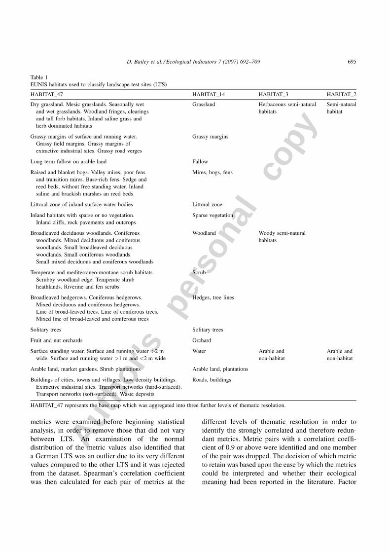
The mapping procedure resulted in digital vector

maps of a high level of detail and complexity. These

maps, henceforth referred to as ‘HABITAT_47’,

represented the base line position and were defined

using a potential of 47 habitat types (Table 1). The

HABITAT_47 maps were reclassified into three

coarser levels of thematic resolution (‘HABITAT_14’,

‘HABITAT_3’ and ‘HABITAT_2’). The HABI-

TAT_14 level had 14 classes, HABITAT_3 maps

aggregated the HABITAT_47 habitats into herbaceous

semi-natural elements, woody semi-natural elements

and arable land, and HABITAT_2 represented a binary

landscape comprising of semi-natural elements

embedded in an arable matrix. The average number

of EUNIS habitats identified in the HABITAT_47 and

HABITAT_14 maps of the individual LTS was 26 and

12, respectively.

For the calculation of landscape metrics the maps

were converted to a raster format with a cell size of

1 m2. To retain the integrity of the linear elements that

were classified on the borders of patch elements (i.e.

linear elements which were not stand alone features but

formed the edge of a polygon), these line features were

firstly buffered (2 m). The buffers were then intersected

with the polygon layer, which resulted in the lines

remaining intact, and forming 1 m wide linear strips

adjoining the edge of the polygon borders. All linear

elements in the LTS had a standardised width of 1 m,

which of course does not represent reality.

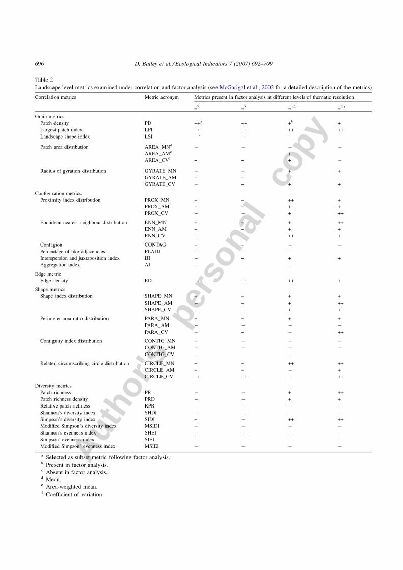
2.2. Landscape Metrics

Forty-one of the most commonly used landscape-

level metrics were selected and calculated in FRAG-

STATS 3.3 (McGarigal et al., 2002). These roughly

represented five main aspects of landscape structure,

namely ‘grain’, ‘edge’, ‘shape’, ‘configuration’ and

‘diversity’ (Table 2). Metrics designed to measure the

core area of patches or the contrast between patches

were excluded from the analyses as they require the

user to define specific weightings related to a

particular ecological process.

To obtain a subset of metrics for each level of

thematic resolution an exploratory approach was

adopted (Riitters et al., 1995), combining correlation

and factor analysis. The values of the individual

D. Bailey et al. / Ecological Indicators 7 (2007) 692–709694

Autho

r's

pers

onal

co

py

metrics were examined before beginning statistical

analysis, in order to remove those that did not vary

between LTS. An examination of the normal

distribution of the metric values also identified that

a German LTS was an outlier due to its very different

values compared to the other LTS and it was rejected

from the dataset. Spearman’s correlation coefficient

was then calculated for each pair of metrics at the

different levels of thematic resolution in order to

identify the strongly correlated and therefore redun-

dant metrics. Metric pairs with a correlation coeffi-

cient of 0.9 or above were identified and one member

of the pair was dropped. The decision of which metric

to retain was based upon the ease by which the metrics

could be interpreted and whether their ecological

meaning had been reported in the literature. Factor

D. Bailey et al. / Ecological Indicators 7 (2007) 692–709 695

Table 1

EUNIS habitats used to classify landscape test sites (LTS)

HABITAT_47 HABITAT_14 HABITAT_3 HABITAT_2

Dry grassland. Mesic grasslands. Seasonally wet

and wet grasslands. Woodland fringes, clearings

and tall forb habitats. Inland saline grass and

herb dominated habitats

Grassland Herbaceous semi-natural

habitats

Semi-natural

habitat

Grassy margins of surface and running water.

Grassy field margins. Grassy margins of

extractive industrial sites. Grassy road verges

Grassy margins

Long term fallow on arable land Fallow

Raised and blanket bogs. Valley mires, poor fens

and transition mires. Base-rich fens. Sedge and

reed beds, without free standing water. Inland

saline and brackish marshes an reed beds

Mires, bogs, fens

Littoral zone of inland surface water bodies Littoral zone

Inland habitats with sparse or no vegetation.

Inland cliffs, rock pavements and outcrops

Sparse vegetation

Broadleaved deciduous woodlands. Coniferous

woodlands. Mixed deciduous and coniferous

woodlands. Small broadleaved deciduous

woodlands. Small coniferous woodlands.

Small mixed deciduous and coniferous woodlands

Woodland Woody semi-natural

habitats

Temperate and mediterraneo-montane scrub habitats.

Scrubby woodland edge. Temperate shrub

heathlands. Riverine and fen scrubs

Scrub

Broadleaved hedgerows. Coniferous hedgerows.

Mixed deciduous and coniferous hedgerows.

Line of broad-leaved trees. Line of coniferous trees.

Mixed line of broad-leaved and coniferous trees

Hedges, tree lines

Solitary trees Solitary trees

Fruit and nut orchards Orchard

Surface standing water. Surface and running water >2 m

wide. Surface and running water >1 m and <2 m wide

Water Arable and

non-habitat

Arable and

non-habitat

Arable land, market gardens. Shrub plantations Arable land, plantations

Buildings of cities, towns and villages. Low density buildings.

Extractive industrial sites. Transport networks (hard-surfaced).

Transport networks (soft-surfaced). Waste deposits

Roads, buildings

HABITAT_47 represents the base map which was aggregated into three further levels of thematic resolution.

Autho

r's

pers

onal

co

py

D. Bailey et al. / Ecological Indicators 7 (2007) 692–709696

Table 2

Landscape level metrics examined under correlation and factor analysis (see McGarigal et al., 2002 for a detailed description of the metrics)

Correlation metrics Metric acronym Metrics present in factor analysis at different levels of thematic resolution

_2 _3 _14 _47

Grain metrics

Patch density PD ++a ++ +b +

Largest patch index LPI ++ ++ ++ ++

Landscape shape index LSI �c � � �

Patch area distribution AREA_MNd � � � �AREA_AMe +

AREA_CVf + + + �

Radius of gyration distribution GYRATE_MN � + + +

GYRATE_AM + + � �GYRATE_CV � + + +

Configuration metrics

Proximity index distribution PROX_MN + + ++ +

PROX_AM + + + +

PROX_CV � � + ++

Euclidean nearest-neighbour distribution ENN_MN + + + ++

ENN_AM + + + +

ENN_CV + + ++ +

Contagion CONTAG + + � �Percentage of like adjacencies PLADJ � � � �Interspersion and juxtaposition index IJI � + + +

Aggregation index AI � � � �Edge metric

Edge density ED ++ ++ ++ +

Shape metrics

Shape index distribution SHAPE_MN + + + +

SHAPE_AM � + + ++

SHAPE_CV + + + +

Perimeter-area ratio distribution PARA_MN + + + +

PARA_AM � � � �PARA_CV � + � ++

Contiguity index distribution CONTIG_MN � � � �CONTIG_AM � � � �CONTIG_CV � � � �

Related circumscribing circle distribution CIRCLE_MN + + ++ ++

CIRCLE_AM + + � +

CIRCLE_CV ++ ++ � ++

Diversity metrics

Patch richness PR � � + ++

Patch richness density PRD � � + +

Relative patch richness RPR � � � �Shannon’s diversity index SHDI � � � �Simpson’s diversity index SIDI + � ++ ++

Modified Simpson’s diversity index MSIDI � � � �Shannon’s evenness index SHEI � � � �Simpson’ evenness index SIEI � � � �Modified Simpson’ evenness index MSIEI � � � �a Selected as subset metric following factor analysis.b Present in factor analysis.c Absent in factor analysis.d Mean.e Area-weighted mean.f Coefficient of variation.

Autho

r's

pers

onal

co

py

analyses were then conducted using the varimax

rotation method with Kaiser normalisation (Backhaus

et al., 2000). To identify the most useful subset of

metrics at each level of thematic resolution, the metric

with the highest factor loading within each factor that

had an eigenvalue �1 were selected. To identify

groups of LTS with similar landscape pattern

characteristics, cluster analyses were undertaken

using the values of the three metrics that represented

the first three factors. With the exception of the cluster

analyses, which were undertaken in STATISTICA 6,

all other analyses were performed using SPSS.

3. Results

The number of habitat types actually recorded in

individual LTS ranged between 21 (in a French LTS)

and 34 (in a Belgium and a Swiss LTS). The arable

matrix made up between 44 and 88% of the LTS’ total

area, followed by herbaceous semi-natural habitats

(1.3–32.3%) and woody semi-natural habitats (1.5–

27.8%). Woodland and grassland were the most

prominent semi-natural elements, followed by ele-

ments such as grassy margins, hedgerows, heath and

scrubland, etc.

3.1. Correlation and factor analysis

The examination of the values of all 41 metrics

prior to statistical analyses led to the rejection of three

metrics from the HABITAT_2 and HABITAT_3

datasets (PR, PRD and RPR; see Table 2 for

explanation of metric acronyms), as they did not vary

between LTS. In addition, IJI was not available at the

HABITAT_2 resolution as it is not calculable in binary

landscapes. The percentage of pairs that were

significantly correlated in the analyses was 34.74%

(HABITAT_2), 32.57% (HABITAT_3), 26.21%

(HABITAT_14) and 24.14% (HABITAT_47). The

diversity metrics were highly correlated with each

other and with CONTAG, a configuration metric at all

levels of thematic resolution. Amongst the grain

metrics, PD and AREA, LPI and AREA and AREA

and GYRATE were strongly correlated at all levels of

thematic resolution. The same applied to the config-

uration metrics, AI and PLADJ, as well as to the shape

metrics PARA and CONTIG. The shape metrics

(PARA and CONTIG) were observed to be highly

correlated with both grain (LSI) and edge (ED); the

configuration metrics (AI, PLADJ) with shape

(PARA, CONTIG), grain (LSI) and edge metrics

(ED); the grain metric LSI with the edge metric ED.

The metrics that were retained for the factor

analyses are listed in Table 2 and the results are

detailed in Table 3. The number of individual factors,

that had eigenvalues �1, ranged from six (HABI-

TAT_2, _3, _14) to eight (HABITAT_47). Cumula-

tively, these factors explained between 84 and 89% of

the variation in the landscape pattern described by the

metrics at each level of thematic resolution.

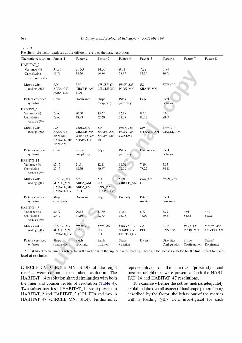
3.2. Metric subsets

To identify the subsets of landscape metrics that

discriminate between the different aspects of pattern

of European agricultural landscapes, we selected the

metric with the highest factor loading for each factor.

To check whether these metrics were able to

discriminate between the LTS we plotted the values

of the indices calculated in FRAGSTATS against the

factor scores calculated for the LTS during the factor

analysis. Only the metrics that distributed the LTS

along a gradient, were retained in the subset (e.g.

CIRCLE_CV, see Fig. 1a). Metrics that only

discriminated the difference between one LTS and

the rest (e.g. ENN_CV, Fig. 1b, PROX_MN and

PROX_AM at the HABITAT_2 and HABITAT_3

levels) were rejected. The final subsets ranged

between four and eight metrics depending on the

thematic level of resolution (Table 4).

There was no one metric that was common to all

thematic resolutions. However, a representative of

‘circle’ was present in each subset. The coefficient of

variation of the metrics (_CV) and the mean (_MN) of

the patch metrics for the entire landscape were the

most common distribution statistics to be present at

each level. Metric subsets were only the same at the

HABITAT_2 and HABITAT_3 level of resolution.

CIRCLE_CV, which had only been available in three

of the factor analysis datasets, was retained in each

case as a subset metric. SIDI was, as might be

expected, retained in both the more complicated

classification systems.

The HABITAT_47 metric subset differed the most

from the other levels of resolution, as only three

D. Bailey et al. / Ecological Indicators 7 (2007) 692–709 697

Autho

r's

pers

onal

co

py

(CIRCLE_CV, CIRCLE_MN, SIDI) of the eight

metrics were common to another resolution. The

HABITAT_14 resolution shared similarities with both

the finer and coarser levels of resolution (Table 4).

Two subset metrics of HABITAT_14 were present in

HABITAT_2 and HABITAT_3 (LPI, ED) and two in

HABITAT_47 (CIRCLE_MN, SIDI). Furthermore,

representatives of the metrics ‘proximity’ and

‘nearest-neighbour’ were present at both the HABI-

TAT_14 and HABITAT_47 resolutions.

To examine whether the subset metrics adequately

explained the overall aspect of landscape pattern being

described by the factor, the behaviour of the metrics

with a loading �0.7 were investigated for each

D. Bailey et al. / Ecological Indicators 7 (2007) 692–709698

Table 3

Results of the factor analyses at the different levels of thematic resolution

Thematic resolution Factor 1 Factor 2 Factor 3 Factor 4 Factor 5 Factor 6 Factor 7 Factor 8

HABITAT_2

Variance (%) 31.76 20.53 14.37 9.51 7.22 6.54

Cumulative

variance (%)

31.76 52.29 66.66 76.17 83.39 89.93

Metrics with

loading �0.7

PDa LPI CIRCLE_CV PROX_AM ED ENN_CV

AREA_CV CIRCLE_AM CIRCLE_MN PROX_MN SHAPE_MN

PARA_MN SIDI

Pattern described

by factor

Grain Dominance Shape

complexity

Patch

proximity

Edge Patch

isolation

HABITAT_3

Variance (%) 28.63 20.30 13.27 12.15 8.77 5.96

Cumulative

variance (%)

28.63 48.93 62.20 74.35 83.12 89.08

Metrics with

loading �0.7

PD CIRCLE_CV ED PROX_MN LPI ENN_CV

AREA_CV CIRCLE_MN SHAPE_AM PROX_AM GYRATE_AM CIRCLE_AM

ENN_MN GYRATE_CV SHAPE_MN CONTAG

GYRATE_MN SHAPE_CV IJI

ENN_AM

Pattern described

by factor

Grain Shape

complexity

Edge Patch

proximity

Dominance Patch

isolation

HABITAT_14

Variance (%) 27.15 21.61 12.21 10.02 7.29 5.85

Cumulative

variance (%)

27.15 48.76 60.97 70.98 78.27 84.13

Metrics with

loading �0.7

CIRCLE_MN LPI ED SIDI ENN_CV PROX_MN

SHAPE_MN AREA_AM PD CIRCLE_AM IJI

GYRATE_MN AREA_CV ENN_MN

GYRATE_CV PRD SHAPE_AM

Pattern described

by factor

Shape

complexity

Dominance Edge Diversity Patch

isolation

Patch

proximity

HABITAT_47

Variance (%) 20.72 20.44 11.79 11.61 8.53 6.32 4.91 4.40

Cumulative

variance (%)

20.72 41.16 52.95 64.55 73.09 79.41 84.32 88.72

Metrics with

loading �0.7

CIRCLE_MN PROX_CV ENN_MN CIRCLE_CV PR SIDI PARA_CV SHAPE_AM

SHAPE_MN LPI PD SHAPE_CV PRD ENN_CV PROX_MN CONTIG_AM

GYRATE_CV ED CONTIG_CV

Pattern described

by factor

Shape

complexity

Patch

proximity

Patch

isolation

Shape

variation

Diversity Diversity/

Configuration

Shape/

Configuration

Shape/

Dominance

a First listed metric under each factor is the metric with the highest factor loading. These are the metrics selected for the final subset for each

level of resolution.

Autho

r's

pers

onal

co

py

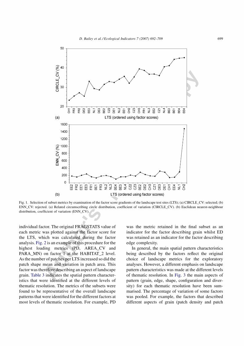
individual factor. The original FRAGSTATS value of

each metric was plotted against the factor score for

the LTS, which was calculated during the factor

analysis. Fig. 2 is an example of this procedure for the

highest loading metrics (PD, AREA_CV and

PARA_MN) on factor 1 at the HABITAT_2 level.

As the number of patches per LTS increased so did the

patch shape mean and variation in patch area. This

factor was therefore describing an aspect of landscape

grain. Table 3 indicates the spatial pattern character-

istics that were identified at the different levels of

thematic resolution. The metrics of the subsets were

found to be representative of the overall landscape

patterns that were identified for the different factors at

most levels of thematic resolution. For example, PD

was the metric retained in the final subset as an

indicator for the factor describing grain whilst ED

was retained as an indicator for the factor describing

edge complexity.

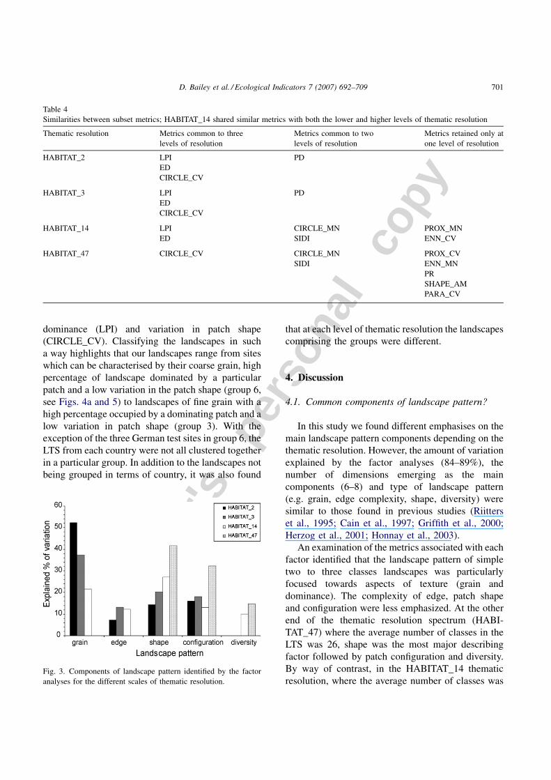
In general, the main spatial pattern characteristics

being described by the factors reflect the original

choice of landscape metrics for the exploratory

analyses. However, a different emphasis on landscape

pattern characteristics was made at the different levels

of thematic resolution. In Fig. 3 the main aspects of

pattern (grain, edge, shape, configuration and diver-

sity) for each thematic resolution have been sum-

marised. The percentage of variation of some factors

was pooled. For example, the factors that described

different aspects of grain (patch density and patch

D. Bailey et al. / Ecological Indicators 7 (2007) 692–709 699

Fig. 1. Selection of subset metrics by examination of the factor score gradients of the landscape test sites (LTS); (a) CIRCLE_CV: selected; (b)

ENN_CV: rejected. (a) Related circumscribing circle distribution, coefficient of variation (CIRCLE_CV). (b) Euclidean nearest-neighbour

distribution, coefficient of variation (ENN_CV).

Autho

r's

pers

onal

co

py

dominance), configuration (patch isolation and patch

proximity), shape (complexity and variation) and

diversity (patch richness, diversity) were combined.

Grain characteristics were highlighted at our lowest

levels of thematic resolution (HABITAT_2, HABI-

TAT_3) whilst shape and configuration explained

more of the spatial pattern variation in our most

complex resolution (HABITAT_47). In comparison,

no one aspect of spatial pattern dominated the

description of landscape pattern at the HABITAT_14

level and all the aspects of pattern were represented.

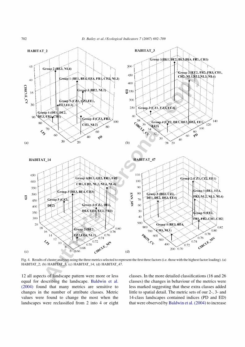
3.3. Subset metrics as indicators of common

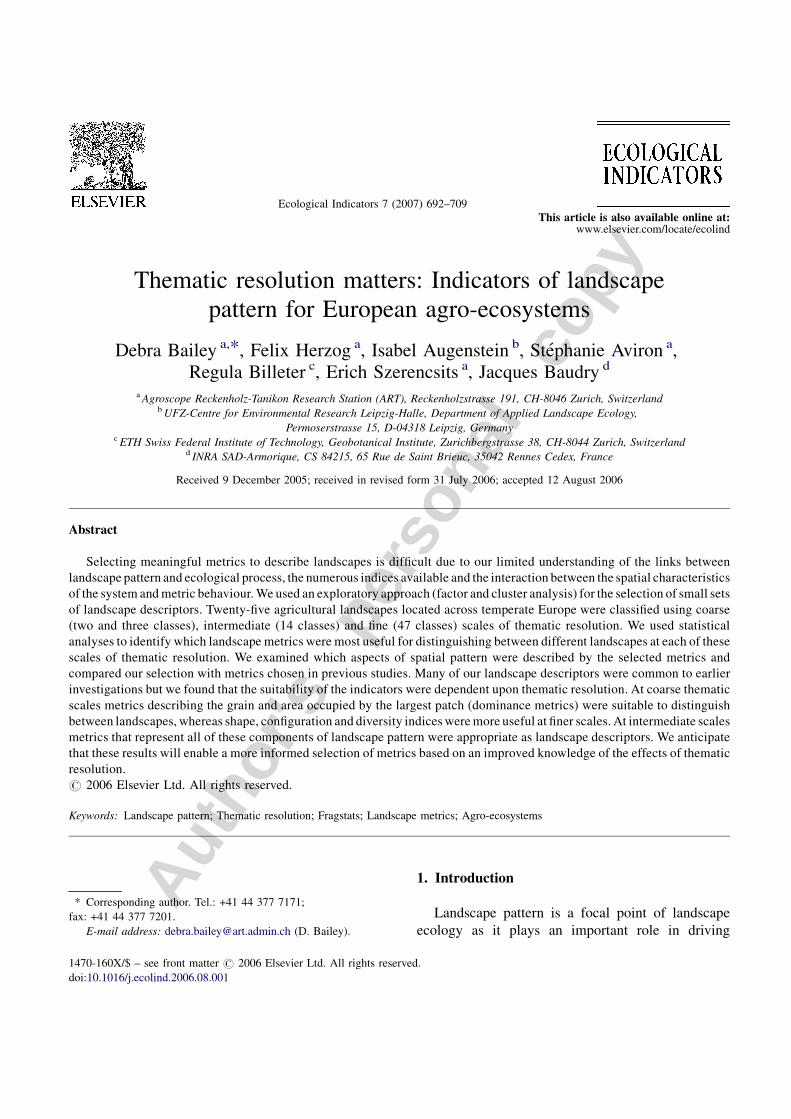
landscape pattern

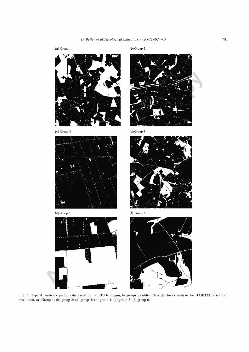
LTS of similar landscape pattern were grouped by

means of a cluster analysis (Fig. 4) and were found to

identify different landscape patterns (Fig. 5). The

results suggest that the three metrics that represented

the factors explaining the most variance were effective

at grouping landscapes into those which show similar

aspects of landscape pattern. For example in Fig. 4a

the LTS are organised according to grain (PD), patch

D. Bailey et al. / Ecological Indicators 7 (2007) 692–709700

Fig. 2. Interpreting landscape pattern. Gradients of pattern described by metrics on factor 1 of the HABITAT_2 level of thematic resolution. (a)

Patch density (PD). (b) Patch area distribution, coefficient of variation (AREA_CV). (c) Perimeter-area ratio distribution (PARA_MN).

Autho

r's

pers

onal

co

py

dominance (LPI) and variation in patch shape

(CIRCLE_CV). Classifying the landscapes in such

a way highlights that our landscapes range from sites

which can be characterised by their coarse grain, high

percentage of landscape dominated by a particular

patch and a low variation in the patch shape (group 6,

see Figs. 4a and 5) to landscapes of fine grain with a

high percentage occupied by a dominating patch and a

low variation in patch shape (group 3). With the

exception of the three German test sites in group 6, the

LTS from each country were not all clustered together

in a particular group. In addition to the landscapes not

being grouped in terms of country, it was also found

that at each level of thematic resolution the landscapes

comprising the groups were different.

4. Discussion

4.1. Common components of landscape pattern?

In this study we found different emphasises on the

main landscape pattern components depending on the

thematic resolution. However, the amount of variation

explained by the factor analyses (84–89%), the

number of dimensions emerging as the main

components (6–8) and type of landscape pattern

(e.g. grain, edge complexity, shape, diversity) were

similar to those found in previous studies (Riitters

et al., 1995; Cain et al., 1997; Griffith et al., 2000;

Herzog et al., 2001; Honnay et al., 2003).

An examination of the metrics associated with each

factor identified that the landscape pattern of simple

two to three classes landscapes was particularly

focused towards aspects of texture (grain and

dominance). The complexity of edge, patch shape

and configuration were less emphasized. At the other

end of the thematic resolution spectrum (HABI-

TAT_47) where the average number of classes in the

LTS was 26, shape was the most major describing

factor followed by patch configuration and diversity.

By way of contrast, in the HABITAT_14 thematic

resolution, where the average number of classes was

D. Bailey et al. / Ecological Indicators 7 (2007) 692–709 701

Fig. 3. Components of landscape pattern identified by the factor

analyses for the different scales of thematic resolution.

Table 4

Similarities between subset metrics; HABITAT_14 shared similar metrics with both the lower and higher levels of thematic resolution

Thematic resolution Metrics common to three

levels of resolution

Metrics common to two

levels of resolution

Metrics retained only at

one level of resolution

HABITAT_2 LPI PD

ED

CIRCLE_CV

HABITAT_3 LPI PD

ED

CIRCLE_CV

HABITAT_14 LPI CIRCLE_MN PROX_MN

ED SIDI ENN_CV

HABITAT_47 CIRCLE_CV CIRCLE_MN PROX_CV

SIDI ENN_MN

PR

SHAPE_AM

PARA_CV

Autho

r's

pers

onal

co

py

12 all aspects of landscape pattern were more or less

equal for describing the landscape. Baldwin et al.

(2004) found that many metrics are sensitive to

changes in the number of attribute classes. Metric

values were found to change the most when the

landscapes were reclassified from 2 into 4 or eight

classes. In the more detailed classifications (16 and 26

classes) the changes in behaviour of the metrics were

less marked suggesting that these extra classes added

little to spatial detail. The metric sets of our 2-, 3- and

14-class landscapes contained indices (PD and ED)

that were observed by Baldwin et al. (2004) to increase

D. Bailey et al. / Ecological Indicators 7 (2007) 692–709702

Fig. 4. Results of cluster analyses using the three metrics selected to represent the first three factors (i.e. those with the highest factor loading). (a)

HABITAT_2; (b) HABITAT_3; (c) HABITAT_14; (d) HABITAT_47.

Autho

r's

pers

onal

co

py

D. Bailey et al. / Ecological Indicators 7 (2007) 692–709 703

Fig. 5. Typical landscape patterns displayed by the LTS belonging to groups identified through cluster analysis for HABITAT_2 scale of

resolution. (a) Group 1; (b) group 2; (c) group 3; (d) group 4; (e) group 5; (f) group 6.

Autho

r's

pers

onal

co

py

rapidly in value with thematic resolution. The

sensitivity of these indices to change in thematic

resolution could explain why these metrics were

selected as descriptors for HABITAT_2 and HABI-

TAT_3 scale as well as at the HABITAT_14 level for

the ED metric. As observed by Baldwin et al. (2004),

the LPI value measured for the different thematic

resolutions, decreased as the number of habitat classes

increased. Potentially the increased subdivision of the

landscape into more classes’ results in a more complex

spatial distribution of patches combined with an

evening in grain between landscapes and results in

other discriminating factors such as patch shape and

distribution gaining in importance.

This study suggests that different metric sets are

required to discriminate the pattern of landscapes

classified using different thematic resolutions. Only

three of the subset metrics (LPI, ED, CIRCLE_CV)

were common to three levels of thematic resolution

and one metric group (circle) to all four scales.

Overall, the metric subsets were only found to be

identical where the magnitude of difference between

the classification systems was relatively small.

The cluster analyses demonstrate further how

thematic resolution influences the grouping of

European agricultural landscapes into similar aspects

of landscape pattern. As the three key metrics used in

the cluster analyses vary between scales of thematic

resolution, different groupings of landscapes are

obtained depending on the scale of resolution. This

is a reflection of the use of different metrics to describe

the LTS and thus the variation in the main aspects of

landscape pattern being described in accordance with

the scale of thematic resolution. The fact that the

clusters of LTS varied depending on thematic

resolution and furthermore were not simply groups

of the same European countries demonstrates the

impact of the use of different landscape classification

systems. Thus, when characterising landscapes

according to their spatial structure and pattern it is

important that consistent maps are used and that the

metrics are appropriate for the thematic resolution.

4.2. Common metrics?

The need to undertake landscape pattern research

under different situations such as varying the spatial

scales and landscapes in the analysis has been stressed

by previous authors (Riitters et al., 1995; Li and Wu,

2004). Only by doing so can it be confirmed whether

similar metrics are consistently useful. From the

literature it is apparent that certain metrics such as

AREA, LSI, CONTAG, LPI, PD, IJI, AWMPFD (area

weighted mean patch fractal dimension), PARA and

SIDI are commonly selected (Riitters et al., 1995;

Cain et al., 1997; Hargis et al., 1998; Griffith et al.,

2000; Herzog et al., 2001; Egbert et al., 2002; Lausch

and Herzog, 2002; Luck and Wu, 2002; Thompson

and McGarigal, 2002; Honnay et al., 2003; Arnot

et al., 2004). With the exception of AWMPFD, which

could not be calculated on our maps, these metrics

were included in our study and a number of them were

selected in our analyses; for example, LPI, PD and

SIDI. Furthermore, the PD and ED metrics of this

study might be representative of AREA and LSI

identified in previous studies. In the correlation

analyses, both AREA and PD together with LSI and

ED were highly correlated. PD and ED were selected

for the factor analyses because they were considered

easier to interpret. Both metrics were found to be

useful discriminators at two (PD) and three (ED)

levels of thematic resolution. In this study CONTAG

was not used in the factor analysis as it was highly

correlated with the diversity indices. Griffith et al.

(2000) kept both CONTAG and the diversity indices

in their analysis of landscape structure but subse-

quently found that the diversity indices were better

correlated with aspects of landscape pattern than

CONTAG. The commonly used IJI metric proved to

be a poor discriminating factor for pattern in our

landscapes with a factor loading below 0.7 in the

factor analyses.

Other metrics also mentioned by other authors were

identified in our subsets. For example, in common

with Herzog et al. (2001) the metric PR was selected in

our most complex classification system. The nearest

neighbour distance was also a subset metric at the

HABITAT_14 and HABITAT_47 levels of classifica-

tion. Previously, Griffith et al. (2000) observed that

nearest neighbour measures could prove useful for the

purposes of landscape monitoring and Hargis et al.

(1998) suggested that they should be added to a

minimal subset of metrics. However, in our results, as

in those of Griffith et al. (2000), the nearest-neighbour

metrics were found to be associated with a factor that

explained little variance. Arnot et al. (2004) have also

D. Bailey et al. / Ecological Indicators 7 (2007) 692–709704

Autho

r's

pers

onal

co

py

examined this index in association with ecotones and

found its behaviour to be extremely variable.

Further metrics, which were identified in our metric

subsets such as CIRCLE, SHAPE, PROX_MN and

PROX_CV, have not been as widely used in other

exploratory analysis studies. Whilst SHAPE was only

part of the metric set at the HABITAT_47 level, the

CIRCLE metric featured as a describing factor in all

scales of thematic resolution. Shape indices have been

examined in a number of studies (e.g., Krummel et al.,

1987; Moser et al., 2002; Saura and Carballal, 2004).

For example, the circle index was observed by Saura

and Carballal (2004) to perfectly discriminate

between native and exotic forest patterns. They

suggested that shape indices not only have potential

to assign the degree of naturality to forested areas but

may also act as indicators of forest biodiversity from a

landscape perspective. The use of shape complexity

indices as indicators of biodiversity is based on the

assumption that landscape shape complexity is

affected by the degree of land-use intensity and hence

geometric landscape complexity will be highly

correlated with biodiversity. Moser et al. (2002) have

already identified that shape complexity is a good

predictor of bryophytes and vascular plant species

richness in Austrian agricultural landscapes. There-

fore, a shape metric such as CIRCLE could prove to be

a useful addition to metric core sets for describing both

landscape pattern and predicting biodiversity.

The proximity indices were descriptors at the

HABITAT_14 and HABITAT_47 level. They were

also present in the HABITAT_2 and HABITAT_3

classification systems but were rejected as they were

found to discriminate only the difference between one

LTS and the rest. In their review of landscape metrics

commonly used to study habitat fragmentation, Hargis

et al. (1998) recommended that an inter-patch measure

should be included to the metric group suggested by

Riitters et al. (1995). Proximity and nearest neighbour

metrics were suggested because although they have

limitations, both have low correlations with other

metrics. However, due to the apparent sensitivity to

thematic resolution they are probably only suited for

use in more complexly defined landscapes.

In general, the _CV and _MN distribution statistics

of the metric were found to have higher factor loadings

in the analyses than the area weighted mean. Gustafson

(1998) has suggested that the use of the mean and

variance for the calculation of patch based metrics at the

class level might be misleading where the distribution

of patch sizes is greatly skewed towards smaller patch

sizes and that area weighted means or medians might

provide better estimates of the central tendency.

However, although included in our landscape level

analyses the area weighted mean was only found at the

HABITAT_47 thematic level of resolution. Here, the

possibility of patch size distribution being skewed, is

perhaps greater due to the higher number of patches,

however in this case it was found to describe very little

variation (4.4%) on one factor.

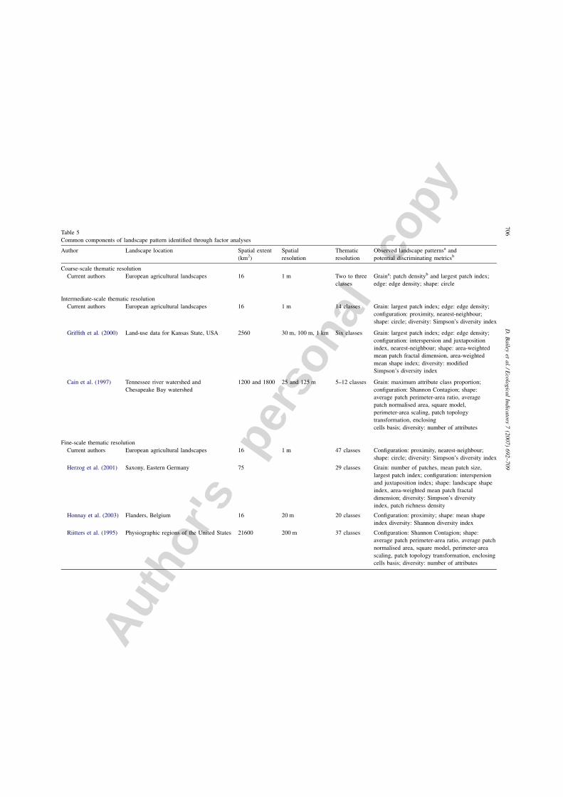
Table 5 summarises the main areas of landscape

pattern and landscape metrics that have emerged from

this and previous exploratory investigations and orders

the results according to coarse-, intermediate- and

fine-scales of thematic resolution. Although the nature

of the spatial heterogeneity measured in a landscape

will ultimately depend on the variables selected for a

study (Li and Reynolds, 1994; Griffith et al., 2000), all

investigations measured common areas of landscape

pattern and identified similar metrics at the different

thematic scales. At the low levels of thematic

resolution, metrics describing the grain and dom-

inance of habitats are more useful for distinguishing

between landscapes of different pattern compared to

the shape, configuration and diversity indices at the

much finer scales. An intermediate scale of thematic

resolution results in metrics that represent all of these

landscape components. Grain metrics were also

selected by Herzog et al. (2001) for the fine-scale

of thematic resolution. However, they undertook a

separate factor analysis for metric groups representing

different areas of landscape pattern (grain, shape,

diversity and configuration) rather than including all

aspects of pattern in the same factor analysis.

4.3. Suitability?

The exploratory method of metric selection enables

the identification of metrics that are able to discriminate

independent components of landscape pattern. There is,

of course, a certain amount of subjectivity in the

selection, as the final subset of metrics will depend on

which indices were included in the initial analysis (Li

and Reynolds, 1994; Griffith et al., 2000). Naturally,

just because the final subsets act as good descriptors of

landscape pattern does not mean that they will also have

D. Bailey et al. / Ecological Indicators 7 (2007) 692–709 705

Autho

r's

pers

onal

co

py

D.

Bailey

etal./E

colo

gica

lIn

dica

tors

7(2

007)

692–709

706Table 5

Common components of landscape pattern identified through factor analyses

Author Landscape location Spatial extent

(km2)

Spatial

resolution

Thematic

resolution

Observed landscape patternsa and

potential discriminating metricsb

Coarse-scale thematic resolution

Current authors European agricultural landscapes 16 1 m Two to three

classes

Graina: patch densityb and largest patch index;

edge: edge density; shape: circle

Intermediate-scale thematic resolution

Current authors European agricultural landscapes 16 1 m 14 classes Grain: largest patch index; edge: edge density;

configuration: proximity, nearest-neighbour;

shape: circle; diversity: Simpson’s diversity index

Griffith et al. (2000) Land-use data for Kansas State, USA 2560 30 m, 100 m, 1 km Six classes Grain: largest patch index; edge: edge density;

configuration: interspersion and juxtaposition

index, nearest-neighbour; shape: area-weighted

mean patch fractal dimension, area-weighted

mean shape index; diversity: modified

Simpson’s diversity index

Cain et al. (1997) Tennessee river watershed and

Chesapeake Bay watershed

1200 and 1800 25 and 125 m 5–12 classes Grain: maximum attribute class proportion;

configuration: Shannon Contagion; shape:

average patch perimeter-area ratio, average

patch normalised area, square model,

perimeter-area scaling, patch topology

transformation, enclosing

cells basis; diversity: number of attributes

Fine-scale thematic resolution

Current authors European agricultural landscapes 16 1 m 47 classes Configuration: proximity, nearest-neighbour;

shape: circle; diversity: Simpson’s diversity index

Herzog et al. (2001) Saxony, Eastern Germany 75 29 classes Grain: number of patches, mean patch size,

largest patch index; configuration: interspersion

and juxtaposition index; shape: landscape shape

index, area-weighted mean patch fractal

dimension; diversity: Simpson’s diversity

index, patch richness density

Honnay et al. (2003) Flanders, Belgium 16 20 m 20 classes Configuration: proximity; shape: mean shape

index diversity: Shannon diversity index

Riitters et al. (1995) Physiographic regions of the United States 21600 200 m 37 classes Configuration: Shannon Contagion; shape:

average patch perimeter-area ratio, average patch

normalised area, square model, perimeter-area

scaling, patch topology transformation, enclosing

cells basis; diversity: number of attributes

Autho

r's

pers

onal

co

py

ecological relevance. In general, there is still a lack of

understanding as to how metrics relate to ecological

process and there is a need for empirical studies that

examine the underlying mechanisms (Wu and Hobbs,

2002; Opdam et al., 2003; Poudevigne and Baudry,

2003). By using a set of metrics that measure

independent factors of pattern at the appropriate

thematic resolution such studies are more likely to

lead to ecological insights.

The inclusion of some class metrics may be

appropriate additions to our metric sets. Class-level

indices have been observed to be better correlated with

ecological response variables than their landscape-

level counterparts and to perform consistently in both

artificial and realistic landscapes (Tischendorf, 2001;

Luck and Wu, 2002). Some metrics identified in this

and previous studies as potential discriminators of

landscape pattern have been observed to provide more

information (e.g. PR, PD, AREA and LSI; Luck and

Wu, 2002) and to explain ecological processes better

(e.g. shape, nearest-neighbour and patch number

metrics; Tischendorf, 2001) at the class rather than

landscape-level.

5. Conclusions

The investigation identified subsets of metrics for

each scale of thematic resolution, enabled us to

recognise main aspects of landscape pattern, facilitated

the compilation of groups of landscapes with similar

characteristics and established which metrics are

frequently useful in landscape studies. Neither the

metric subsets nor the clusters of landscapes were the

same for the different scales of thematic resolution.

Hence, metrics respond to differences in thematic

resolution as well as to changes in spatial extent and

spatial resolution. Therefore, when deciding upon

indices, the behaviour of the metric to thematic

resolution and its relevance to the chosen classification

system should be considered. The use of an exploratory

approach for the selection of landscape-level metrics

should however not exclude the consideration of certain

class metrics, for example those defining landscape

composition (e.g. habitat amount), as these might better

define the pattern and relate it to specific processes. The

thematic scale will also depend on the ecological

question (Suarez-Seoane and Baudry, 2002).

The issue of the sensitivity of many commonly

used metrics to thematic resolution is critical as

landscape ecologists are forced to simplify and define

landscapes in order to investigate them. Our study

confirms that although certain metrics are consistently

chosen through exploratory analysis their selection

depends on the thematic scale. Therefore, in order to

describe spatial structure and patterns, to characterise

landscapes or to classify them to major landscape

types (based on their structure) it is important to take

into account the thematic resolution effect. Based on

the results of this and other studies we would suggest

the inclusion of PD, LPI, ED, CIRCLE and a

landscape composition parameter (e.g. the percentage

of landscape comprised of main land use/cover) for the

study of landscapes of low thematic resolution.

Subsets to examine intermediately defined landscapes

should include LPI and ED as well as a diversity index

(e.g. SIDI or PR), nearest neighbour, shape and

proximity metrics. A landscape composition metric

might also be pertinent depending on the process

under consideration. The emphasis for complexly

defined landscapes should be placed on shape

(CIRCLE), diversity (SIDI and PR) and configuration

(proximity and nearest neighbour) metrics. However,

metrics describing landscape composition (e.g. %

habitat or ED) might be relevant if a specific process or

species (group) is being examined.

An important research issue is whether metrics

commonly selected through exploratory analysis are

useful for the study of biodiversity or other specific

landscape questions. Landscape-level metrics selected

using exploratory techniques might enable an

informed selection of more appropriate class metrics:

an exploratory guided expert approach. We are

currently examining this issue and analyses by

Schweiger et al. (2005) have already confirmed the

importance of composition and configuration indices

such as proximity for the study of different aspects of

agro-ecosystem biodiversity.

Acknowledgements

The European Union (EU-Reference EVK2-CT-

2000-00082) and the Swiss State Secretariat for

Education and Research (SER No. 00.0080-1) funded

part of this research. We thank Riccardo De Filippi and

D. Bailey et al. / Ecological Indicators 7 (2007) 692–709 707

Autho

r's

pers

onal

co

py

Nicolas Schermann for their advice and technical

support, Rob Bugter for his project guidance and

Angela Lausch for her comments on an earlier draft of

the paper.

References

Arnot, C., Fisher, P.F., Wadsworth, R., Wellens, J., 2004. Landscape

metrics with ecotones: pattern under uncertainty. Landsc. Ecol.

19, 181–195.

Baldwin, D.J.B., Weaver, K., Schnekenburger, F., Perera, A.H.,

2004. Sensitivity of landscape pattern indices to input data

characteristics on real landscapes: implications for their use

in natural disturbance emulation. Landsc. Ecol. 19, 255–272.

Backhaus, K., Erichson, B., Plinke, W., Weiber, R., 2000. Multi-

variate Analysemethoden: eine anwendungsorientierte Einfueh-

rung. Springer-Verlag.

Bender, D.J., Tischendorf, L., Fahrig, L., 2003. Using patch isolation

metrics to predict animal movement in binary landscapes.

Landsc. Ecol. 18, 17–39.

Bogaert, J., Myneni, R.B., Knyazikhin, Y., 2002. A mathematical

comment on the formulae for the aggregation index and the

shape index. Landsc. Ecol. 1–4.

Bugter, R.J.F., Burel, F., Cerny, M., Edwards, P.J., Herzog, F.,

Maelfait, J.P., Klotz, S., Simova, P., Smulders, R., Zobel M.,

2001. Vulnerability of biodiversity in the agro-ecosystems as

influenced by green veining and land-use intensity: the EU

project GREENVEINS. In: Mander, U., Printsmann, A., Palang,

H. (Eds.), Development of European Landscapes. Proceedings

of the International Association for Landscape Ecology, vol. 92.

Publicationes Instituti Geographici Universitatis Tartuensis,

Tartu, pp. 632–637.

Cain, D.H., Riitters, K., Orvis, K., 1997. A multi-scale analysis of

landscape statistics. Landsc. Ecol. 12, 199–212.

Davies, C.E., Moss, D., 1999. EUNIS Habitat Classification. Final

Report to the European Topic Centre on Nature Conservation.

European Environment Agency, Paris, 256 pp.

Egbert, S.L., Park, S., Price, K.P., Lee, R., Wu, J., Nellis, D., 2002.

Using conservation reserve program maps derived from satellite

imagery to characterise landscape structure. Comput. Electron.

Agric. 37, 141–156.

Fahrig, L., Jonsen, I., 1998. Effect of habitat patch characteristics on

abundance and diversity of insects in an agricultural landscape.

Ecosystems 1, 197–205.

Forman, R.T.T., Godron, M., 1986. Landscape Ecology. John Wiley

& Sons, New York, USA.

Griffith, J.A., Martunko, E.A., Price, K.P., 2000. Landscape struc-

ture analysis of Kansas at three scales. Landsc. Urban Plann. 52,

45–61.

Gustafson, E.J., 1998. Quantifying landscape spatial pattern: what is

the state of the art? Ecosystems 1, 143–156.

Gustafson, E.J., Parker, G.R., 1994. Using an index of habitat patch

proximity for landscape design. Landsc. Urban Plann. 29, 117–

130.

Hargis, C.D., Bissonette, J.A., David, J.L., 1998. The behaviour of

landscape metrics commonly used in the study of habitat

fragmentation. Landsc. Ecol. 13, 167–186.

Herzog, F., Steiner, B., Bailey, D., Baudry, J., Billeter, R., Bukacek, R.,

De Blust, G., De Cock, R., Dirksen, J., Dormann, C., De Filippi,

R., Frossard, E., Liira, J., Stockli, S., Schmidt, T., Thenail, C., van

Wingerden, W., Bugter, R., 2006. Assessing the intensity of

temperate European agriculture with respect to impacts on land-

scape and biodiversity. Eur. J. Agron. 24, 165–181.

Herzog, F., Lausch, A., Muller, E., Thulke, H., Steinhardt, U.,

Lehmann, S., 2001. Landscape metrics for the assessment of

landscape destruction and rehabilitation. Environ. Manage. 27,

91–107.

Honnay, O., Piessens, K., van Landuyt, W., Hermy, M., Gulinck, H.,

2003. Satellite based land use and landscape complexity indices

as predictors for regional plant species diversity. Landsc. Urban

Plann. 63, 241–250.

Krummel, J.R., Gardner, G., Sugihara, G., O’Neill, R.V., Coleman,

P.R., 1987. Landscape patterns in a disturbed environment.

Oikos 48, 287–297.

Lausch, A., Herzog, F., 2002. Applicability of landscape metrics for

the monitoring of landscape change: issues of scale, resolution

and interpretability. Ecol. Indicators 2, 3–15.

Lawler, J.A., O’Connor, R.J., Hunsaker, C.T., Jones, K.B., Love-

land, T.R., White, D., 2004. The effects of habitat resolution on

models of avian diversity and distributions: a comparison of two

land-cover classifications. Landsc. Ecol. 19, 515–530.

Li, H., Reynolds, J.F., 1994. A simulation experiment to quantify

spatial heterogeneity in categorical maps. Ecology 75, 2446–

2455.

Li, H., Wu, J., 2004. Use and misuse of landscape indices. Landsc.

Ecol. 19, 389–399.

Luck, M., Wu, J., 2002. A gradient analysis of urban landscape

pattern: a case study from the Phoenix metropolitan region,

Arizona, USA. Landsc. Ecol. 17, 327–339.

Mazerolle, M.J., Villard, M.A., 1999. Patch characteristics and

landscape context as predictors of species presence and abun-

dance: a review. Ecoscience 6, 117–124.

McGarigal, K., Cushman, S.A., Neel, M.C., Ene, E., 2002. FRAG-

STATS: Spatial Pattern Analysis Program for Categorical Maps.

Computer Software Program Produced by the Authors at the

University of Massachusetts, Amherst. Available at the follow-

ing web site: www.umass.edu/landeco/research/fragstats/frag-

stats.html.

Moser, D., Zechmeister, H.G., Plutzar, C., Sauberer, N., Wrbka, T.,

Grabherr, G., 2002. Landscape patch shape complexity as an

effective measure for plant species richness in rural landscapes.

Landsc. Ecol. 17, 657–669.

Neel, M.C., McGarigal, K., Cushman, S., 2004. Behavior of class-

level metrics across gradients of class aggregation and area.

Landsc. Ecol. 19, 435–455.

O’Neill, R.V., Hunsaker, C.T., Jones, K.B., Riitters, K.H., Wickham,

J.D., Schwartz, P.M., Goodman, I.A., Jackson, B.L., Baillar-

geon, W.S., 1997. Monitoring environmental quality at the

landscape scale. Using landscape indicators to assess biotic

diversity, watershed integrity, and landscape stability.

Bioscience 47, 513–519.

D. Bailey et al. / Ecological Indicators 7 (2007) 692–709708

Autho

r's

pers

onal

co

py

Opdam, P., Verboom, J., Pouwels, R., 2003. Landscape cohesion: an

index for the conservation potential of landscapes for biodiver-

sity. Landsc. Ecol. 18, 113–126.

Poudevigne, I., Baudry, J., 2003. The implication of past and present

landscape patterns for biodiversity research: introduction and

overview. Landsc. Ecol. 18, 223–225.

Riitters, K.H., Wickham, J., O’Neill, R., Jones, B., Smith, E., 2000.

Global-scale patterns of forest fragmentation. Conserv. Ecol. 4,

27–56.

Riitters, K.H., O’Neill, R.V., Hunsacker, C.T., Wickham, J.D.,

Yankee, D.H., Timmins, S.P., Jones, K.B., Jackson, B.L.,

1995. A factor analysis of landscape pattern and structure

metrics. Landsc. Ecol. 10, 23–39.

Saura, S., Carballal, P., 2004. Discrimination of native and exotic

forest patterns through shape irregularity indices: an analysis in

the landscapes of Galicia, Spain. Landsc. Ecol. 19, 647–662.

Schweiger, O., Maelfait, J.P., van Wingerden, W., Hendrickx, F.,

Billeter, R., Speelmans, M., Augenstein, I., Aukema, B., Aviron,

S., Bailey, D., Bukacek, R., Burel, F., Diekotter, T., Dirkens, J.,

Frenzel, M., Herzog, F., Liira, J., Roubalova, M., Bugter, R.,

2005. Quantifying the impact of environmental factors on

arthropod communities in agricultural landscapes across orga-

nisational levels and spatial scales. J. Appl. Ecol. 42, 1129–1139.

Suarez Seoane, S., Baudry, J., 2002. Scale dependence of spatial

patterns and cartography on the detection of landscape change.

Relationships with species’ perception. Ecography 25, 499–511.

Thompson, C.M., McGarigal, K.M., 2002. The influence of research

scale on bald eagle habitat selection along the lower Hudson

River New York (USA). Landsc. Ecol. 17, 569–586.

Tischendorf, L., 2001. Can landscape indices predict ecological

processes consistently? Landsc. Ecol. 16, 235–254.

Turner, M.G., Gardner, R.H., O’Neill, R.V., 2001. Landscape Ecol-

ogy in Theory and Practice: Pattern and Process. Springer-

Verlag, New York, USA.

Turner, M.G., O’Neill, R.V., Gardner, R.H., Milne, B.T., 1989.

Effects of changing spatial scale on the analysis of landscape

pattern. Landsc. Ecol. 3, 153–162.

Wu, J., Hobbs, R., 2002. Key issues and research priorities in

landscape ecology: an idiosyncratic synthesis. Landsc. Ecol.

17, 355–365.

D. Bailey et al. / Ecological Indicators 7 (2007) 692–709 709