The Yield Curve as a Leading Indicator - MDPI

forecasting

Article

The Yield Curve as a Leading Indicator: Accuracy and Timing ofa Parsimonious Forecasting Model

Knut Lehre Seip 1,* and Dan Zhang 2

�����������������

Citation: Seip, K.L.; Zhang, D. The

Yield Curve as a Leading Indicator:

Accuracy and Timing of a

Parsimonious Forecasting Model.

Forecasting 2021, 3, 421–436. https://

doi.org/10.3390/forecast3020025

Academic Editor: Alessia Paccagnini

Received: 20 March 2021

Accepted: 24 May 2021

Published: 28 May 2021

Publisher’s Note: MDPI stays neutral

with regard to jurisdictional claims in

published maps and institutional affil-

iations.

Copyright: © 2021 by the authors.

Licensee MDPI, Basel, Switzerland.

This article is an open access article

distributed under the terms and

conditions of the Creative Commons

Attribution (CC BY) license (https://

creativecommons.org/licenses/by/

4.0/).

1 Art and Design, Faculty of Technology, Oslo Metropolitan University, 0167 Oslo, Norway2 Oslo Business School, Oslo Metropolitan University, 0167 Oslo, Norway; [email protected]* Correspondence: [email protected]; Tel.: +47-67238816

Abstract: Previous studies have shown that the treasury yield curve, T, forecasts upcoming recessionswhen it obtains a negative value. In this paper, we try to improve the yield curve model while keepingits parsimony. First, we show that adding the federal funds rate, FF, to the model, GDP = f(T, FF),gives seven months vs. five months warning time, and it gives a higher prediction skill for therecessions in the out-of-sample test set. Second, we find that including the quadratic term of theyield curve and the federal funds rate improves the prediction of the 1990 recession, but not the otherrecessions in the period 1977 to 2019. Third, the T caused a pronounced false peak in GDP for the testset. Restricting the learning set to periods where T and FF were leading the GDP in the learning setdid not improve the forecast. In general, recessions are predicted better than the general movementin the economy. A “horse race” between GDP = f(T, FF) and the Michigan consumer sentiment indexsuggests that the first beats the latter by being a leading index for the observed GDP for more months(50% vs. 6%) during the first test year.

Keywords: term structure; federal funds interest rate; GDP; forecasting; economic growth; aggre-gate productivity

1. Introduction

An accurate forecast of economic growth and upcoming economic recessions is crucialto households, businesses, investors and policymakers. There is a vast literature onforecasting economic growth and recessions based on macroeconomic indicators, amongwhich the treasury yield curve has often been cited as a leading indicator, with inversion ofthe curve being a signal of a recession. For example, Estrella and Hardouvelis [1], Estrellaand Mishkin [2] and Estrella and Mishkin [3] explained how the yield curve significantlyoutperforms other financial and macroeconomic indicators in predicting recessions two tosix quarters ahead.

Studies also provide empirical evidence showing that the domestic government bondyield spreads are the best recession predictor for output growth and recessions (see, forexample, Duarte, Venetis [4] and Nyberg [5]). In addition, recent studies on predictingrecessions find that the yield curve consistently outperforms even professional forecasterswho have a rich set of indicators and forecasting tools available to them (Rudebusch andWilliams [1] and Croushore and Marsten [6]).

Our analysis differs from earlier studies of forecasting economic growth and recessionsby focusing on both parsimony and the timing and accuracy of the predictions. Recentstudies of forecasting economic growth and recessions often use complex mathematicalmodels and a large set of financial and macroeconomic variables. We examine if thepredictions based on the treasury yield curve can parsimoniously be improved to give alonger warning time and better accuracy. The added value of our study is fivefold. First,we examine the benefit of including the federal funds rate (FF) and its interactions with thetreasury yield curve (T) in a multiple equation regression. Second, we restrict the learning

Forecasting 2021, 3, 421–436. https://doi.org/10.3390/forecast3020025 https://www.mdpi.com/journal/forecasting

Forecasting 2021, 3 422

set to portions of the time series where T and FF lead the GDP. Third, we compare sixpossible models to see which models gives the best prediction of the general movementsand of the five NBER recessions during our study period 1971 to 2019. Fourth, we showvisually how time series predicted with T alone would differ from predictions with FFalone. This allows us to identify events that are caused by a particular variable. Finally, wearrange a “horse race” between our prediction GDP = f(T, FF) and the Michigan consumersentiment index (MCSI), a frequently used index for forecasting movements in the GDPone year ahead.

Predicting business cycles during their general development, and during recessionsand recoveries, is of clear interest to policymakers and market participants. Policymakersmay respond to the forecasts by adjusting their policies for economic expansions andcontractions. They could also use the forecasting model to quantify the economic impactunder different scenarios. Market participants may utilize the forecast to assess risksand adjust their investment strategies accordingly. Our forecasting model that combinesparsimony, predictive accuracy, timing and ease of estimation could benefit policymakersand market participants.

In the rest of the manuscript, we present the literature review and develop the hy-pothesis in Section 2. In Section 3, we describe our data and present the methodology andour testing procedures. The results are shown in Section 4, and we discuss the results inSection 5. Finally, we discuss policy implications and conclude the findings in Section 6.

2. Literature Review and Hypotheses

A large body of literature studies the predictive power of financial and macroeconomicleading indicators for real output growth and recessions. Most prominently, Estrella andHardouvelis [2], Estrella and Mishkin [3] and Estrella and Mishkin [4] documented thatthe slope of the treasury yields curve has strong predictive power for US output growthand US recessions at horizons of up to eight quarters. Chauvet and Potter [7] examinedfurther extensions of the yield curve probit model, including a business cycle-dependentmodel, a model with autocorrelated errors and combinations of these extensions. Theyfound evidence in favor of the more sophisticated models that allows for autocorrelationand multiple breakpoints across business cycles.

In addition to the empirical evidence in the US, other works have documented thestrong predictive power of the government bond yield spreads for output growth andrecessions internationally. For example, Duarte, Venetis and Payà [5] confirmed the abilityof the yield curve as a leading indicator to predict recessions in the European MonetaryUnion. Nyberg [6] examined recessions in the USA and Germany and showed that thedomestic term spread remains the best recession predictor.

While the yield spread has long been recognized as a good predictor of recessions,it seems to have been largely overlooked by professional forecasters. Rudebusch andWilliams [1] found that the yield curve consistently outperforms professional forecastersin predicting recessions. This is puzzling given that professional forecasters have a richset of indicators and forecasting tools available to them. Lahiri, Monokroussos [8] andCroushore and Marsten [7] confirmed that Rudebusch and Williams’s [1] findings arerobust, including augmenting the model with more macroeconomic factors, the use ofdifferent sample periods, the use of rolling regression windows and various alternativemeasures of real output. Yang [9] found the yield curve to have a well-performing abilityto forecast the real GDP growth in the USA, compared to professional forecasters and timeseries models.

In our study, we try to make the best use of the predictive power of the yield curve asdocumented in the literature and ask whether we could improve the yield curve modelwhile keeping the model as parsimonious as possible. We developed four hypothesesthat we will test empirically. Our first hypothesis (H1, the baseline model) is that thetreasury yield curve alone will explain most of the variation in the GDP. All the papers

Forecasting 2021, 3 423

discussed above highlight the singular importance of the treasury yield curve as a predictorof recessions and justify our use of this indicator as the benchmark predictor variable.

Economic growth, recessions and interest rates are all endogenous and any associationamong them could be considered a reduced form correlation. Estrella and Hardouvelis [2]tested a model with both the yield curve and the federal funds rate included. Theirresults showed that a higher real federal funds rate today is associated with a lowergrowth in the future real output. Bauer and Rudebusch [8] documented that accountingfor dynamic changes in the equilibrium short rate is essential for forecasting the yield.Galbraith and Tkacz [9] found that the yield curve–output relation might not be linearand its predictive content might have asymmetric effects. The work by Venetis, Paya andPeel [10] showed that the relationship is stronger when past values of the yield spreaddo not exceed a positive threshold value. Therefore, our second hypothesis, H2, is thatpredictions of the GDP will improve if we augment the yield curve model with the federalfunds rate. Specifically, we will include second-order interactions as additional variablesbecause the T and the FF may give complementary information on the state of the economywhen recessions are not imminent. Furthermore, the relationship between the predictionalgorithm and GDP may not be stable over time and it may be subjected to nonlinearities(see, for example, Galbraith and Tkacz [10] and Venetis, Paya [11]).

Concerns have been raised that the predictive performance of the yield curve modelmay be time-variant, and that predictive regressions based on the yield spread may sufferfrom parameter instability, e.g., Estrella, Rodrigues [12] and Giacomini and Rossi [13].Estrella, Rodrigues [12] studied the United States (and Germany) and showed that there issome evidence of instability in the real growth models for the United States, whereas therecession models are generally stable. Giacomini and Rossi [11] documented the existenceof a forecast breakdown, whereas during the early part of the Greenspan era, the yieldcurve emerged as a more reliable model to predict future economic activity. Therefore,our third hypothesis, H3, is that the explained variances between the predicted and theobserved GDP will be higher if the forecasting models are restricted to the time windowwhere the yield curve and the federal funds rate are leading variables to GDP. The rationaleis that the leading relations between the yield curve, the federal funds rate and GDP maychange with time, e.g., Schrimpf and Wang [14], and in some periods, the informationcarried by the yield curve and the federal funds rate is not available before the marketmakes its decisions. Therefore, it may distort the estimation of the parameters in theprediction equations if we include observations of the independent variables that occurafter the GDP has changed.

Our fourth hypothesis, H4, is that recessions would be better predicted than the overallGDP. The rationale is that Seip, Yilmaz [15] found for the German economy from 1991 to2016 that recessions had a higher probability to be predicted correctly than the overallGDP time series by two German sentiment indexes. In general, there may be periods inthe development of the GDP that are better predicted than others, and algorithms that arerobust across macroeconomic breakpoints should be preferable.

3. Data and Methods3.1. Data

We used the real GDP as a proxy for real economic growth and identified recessionperiods using National Bureau of Economic Research (NBER) definitions. The recessions inthe USA during the period 1977 to 2019 are shown in Table 1.

We measured the yield curve, T, as the difference between the 10-year and 2-yeartreasury bond yields. This is in the maximum maturity spread range. Long ranges werefound to be the best measure of the spread slope by Ang, Plazzesi [16]. We obtained the datafor GDP and the difference between the 10-year constant maturity and the 2-year treasuryconstant maturity from the Federal Reserve Bank of St. Louis (https://fred.stlouisfed.org/series/T10Y2Y, accessed on 20 March 2021). The federal funds rate, FF, was also retrievedfrom the Federal.

Forecasting 2021, 3 424

Table 1. Recessions in the USA, 1970 to 2019.

Recession Key Factors Dates Neg. T LeadsRecession, Months

The 1980 recession The Volcker inflation targeting January 1980–July 1980 19The 1981–1982 recession The 1979 energy crisis July 1981–November 1982 -Early 1990s recession 1990 oil price shock July 1990–March 1991 14

Early 2000s recessionThe dotcom bubble, the 9/11attacks and accounting scandalsat major US corporations

March 2001–November 2001 16

The 2008 recession The subprime mortgage crisis inUS and global financial crisis December 2007–June 2009 21

Average 17.5 ± 3.1

Note: data from NBER, National Bureau of Economic Research.

Reserve Bank of St. Louis (https://fred.stlouisfed.org/series/FEDFUNDS, accessedon 20 March 2021). We used economic data from 1977 to 2019M5 at a monthly frequency,that is, 512 entries. As the GDP data are quarterly, we interpolated the GDP data to monthlydata. We were able to add data from 2019M6 to 2020M4 for GDP and from 2019M6 to2020M8 for T and FF. However, as the 2020 recession is ongoing, we only included therecent data points for comparison purposes.

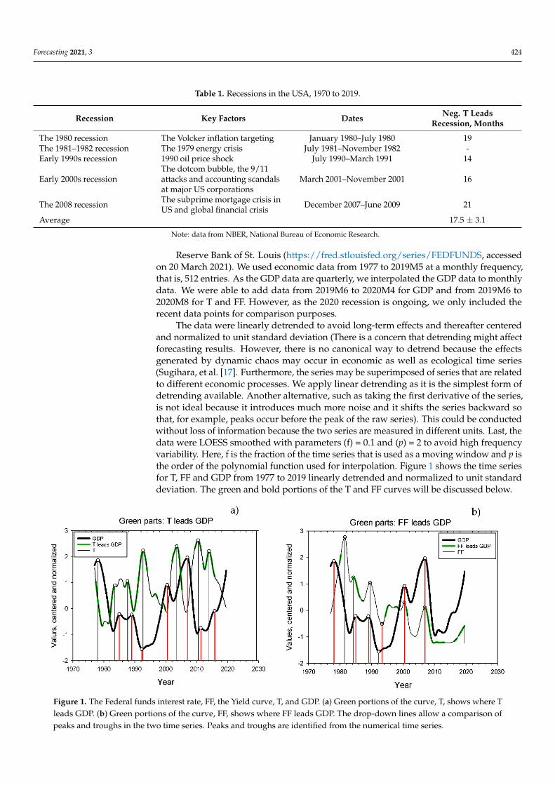
The data were linearly detrended to avoid long-term effects and thereafter centeredand normalized to unit standard deviation (There is a concern that detrending might affectforecasting results. However, there is no canonical way to detrend because the effectsgenerated by dynamic chaos may occur in economic as well as ecological time series(Sugihara, et al. [17]. Furthermore, the series may be superimposed of series that are relatedto different economic processes. We apply linear detrending as it is the simplest form ofdetrending available. Another alternative, such as taking the first derivative of the series,is not ideal because it introduces much more noise and it shifts the series backward sothat, for example, peaks occur before the peak of the raw series). This could be conductedwithout loss of information because the two series are measured in different units. Last, thedata were LOESS smoothed with parameters (f) = 0.1 and (p) = 2 to avoid high frequencyvariability. Here, f is the fraction of the time series that is used as a moving window and p isthe order of the polynomial function used for interpolation. Figure 1 shows the time seriesfor T, FF and GDP from 1977 to 2019 linearly detrended and normalized to unit standarddeviation. The green and bold portions of the T and FF curves will be discussed below.

Forecasting 2021, 3 FOR PEER REVIEW 5

Figure 1. The Federal funds interest rate, FF, the Yield curve, T, and GDP. (a) Green portions of the curve, T, shows where T leads GDP. (b) Green portions of the curve, FF, shows where FF leads GDP. The drop-down lines allow a comparison of peaks and troughs in the two time series. Peaks and troughs are identified from the numerical time series.

3.2.1. Multiple Regression We applied multiple regressions to the independent variables T, T2, FF, FF2 and T ×

FF (Although other methods, such as the probit models, are more commonly used Johans-son and Meldrum [19] Bauer and Mertens [20], these models focus on recession forecasts, whereas we also compare predicted and observed full series. A recent set of studies use the machine learning framework. Gogas et al. [21], Medeiros et al. [22]. Last, we follow Bauer and Mertens [23]. “Information in the Yield Curve about Future Recessions” Re-trieved 17 September 2020, in their adage “correlation is not causation” and examine pos-sible causal links in addition to statistical associations). We conducted regressions with the regressors both shifted and not shifted relative to the dependent GDP.

GDPt = α0 + α1Tt+n + α2T2 t+n + α3FFt+n + α4FF2t+n + α5Tt+n × FFt+n (1)

where αi is the coefficients to be estimated and n = 0 in the zero shifted alternative. We also tried values of n from −1 to −4. We used the multiple regression algorithm as imple-mented in SigmaPlot©.

The predictions with only one variable gave a narrow range of values (≈−1, +1; not shown), but the interesting feature is the differences between the observed and the pre-dicted time series. We therefore normalized the series to unit standard deviation to corre-spond in range with the normalized GDP series before calculating the RMSE. The time lags (months) were calculated as the difference between the predicted and the observed turning points for GDP after the observed GDP time series have been slightly LOESS smoothed (f = 0.1, p = 2) to avoid sharp peaks in the time series.

We divided our data into a learning set, 1977M1-2004M12, and a test set, 2005M1 to 2019M5. The coefficients of the equations were determined by applying the equations to the learning set. The forecasting skill was determined by calculating the RMSE between the calculated and observed time series. Last, we applied the forecasting equations to pe-riods before the five recessions.

3.2.2. Comparing GDP to Forecasts We used two methods to compare GDP to forecasts: the root mean square error

(RMSE), and the adjusted explained variance, R2, of the least square regression. The RMSE would give a measure of the difference between the observed and the predicted GDP over a certain period. The R2 would measure the skill of predicting co-movements between the observed and the predicted GDPs. We also report R to maintain the sign of the regression,

Figure 1. The Federal funds interest rate, FF, the Yield curve, T, and GDP. (a) Green portions of the curve, T, shows where Tleads GDP. (b) Green portions of the curve, FF, shows where FF leads GDP. The drop-down lines allow a comparison ofpeaks and troughs in the two time series. Peaks and troughs are identified from the numerical time series.

Forecasting 2021, 3 425

3.2. Methodology

To identify time windows where the regressors lead the target variable GDP, weapplied a lead–lag method to the time series [15,18]. The green curves in Figure 1a,b showwhere T and FF lead GDP. The drop-down lines show peaks and troughs in the curves.When we restrict the learning set to time windows where either T or FF leads GDP, we usethe results depicted in these graphs.

3.2.1. Multiple Regression

We applied multiple regressions to the independent variables T, T2, FF, FF2 and T× FF(Although other methods, such as the probit models, are more commonly used Johanssonand Meldrum [19] Bauer and Mertens [20], these models focus on recession forecasts,whereas we also compare predicted and observed full series. A recent set of studies use themachine learning framework. Gogas et al. [21], Medeiros et al. [22]. Last, we follow Bauerand Mertens [23]. “Information in the Yield Curve about Future Recessions” Retrieved 17September 2020, in their adage “correlation is not causation” and examine possible causallinks in addition to statistical associations). We conducted regressions with the regressorsboth shifted and not shifted relative to the dependent GDP.

GDPt = α0 + α1Tt+n + α2T2t+n + α3FFt+n + α4FF2

t+n + α5Tt+n × FFt+n (1)

where αi is the coefficients to be estimated and n = 0 in the zero shifted alternative. We alsotried values of n from−1 to−4. We used the multiple regression algorithm as implementedin SigmaPlot©.

The predictions with only one variable gave a narrow range of values (≈−1, +1;not shown), but the interesting feature is the differences between the observed and thepredicted time series. We therefore normalized the series to unit standard deviation tocorrespond in range with the normalized GDP series before calculating the RMSE. The timelags (months) were calculated as the difference between the predicted and the observedturning points for GDP after the observed GDP time series have been slightly LOESSsmoothed (f = 0.1, p = 2) to avoid sharp peaks in the time series.

We divided our data into a learning set, 1977M1-2004M12, and a test set, 2005M1 to2019M5. The coefficients of the equations were determined by applying the equations tothe learning set. The forecasting skill was determined by calculating the RMSE between thecalculated and observed time series. Last, we applied the forecasting equations to periodsbefore the five recessions.

3.2.2. Comparing GDP to Forecasts

We used two methods to compare GDP to forecasts: the root mean square error(RMSE), and the adjusted explained variance, R2, of the least square regression. The RMSEwould give a measure of the difference between the observed and the predicted GDP overa certain period. The R2 would measure the skill of predicting co-movements between theobserved and the predicted GDPs. We also report R to maintain the sign of the regression,and we add a sign for the RMSE to see if the predicted GDP is above or below the observedGDP. First, we evaluated the result by calculating RMSE between the predicted GDP (GDPp)and the observed GDP (GDPo):

RMSE=√

(1/T ∑(GDPp-GDPo)2) (2)

We conducted a tentative test statistic by regressing GDP to a uniform random distribu-tion using the RAND () function in Excel and calculating the RMSE. Using an autoregressiveAR (1) model made the RMSE statistics, on average, larger and worse. We did this for thefull series 1977M1 to 2019M5, RMSE (GDP512, R512), the test set 2005M1 to 2019M5, RMSE(GDP175, R175), and for 20 months before the five recessions, RMSE (GDP20, R20). Wedid this 10 times and calculated the average and standard deviation of the RMSE. Last, we

Forecasting 2021, 3 426

calculated the RMSE for two stochastic series of the same length as our full time series,RMSE (R512, R512).

The forecasting horizons in our study are 197 to 336 months for the learning set,175 months for the test set and 20 months for the periods before the recessions.

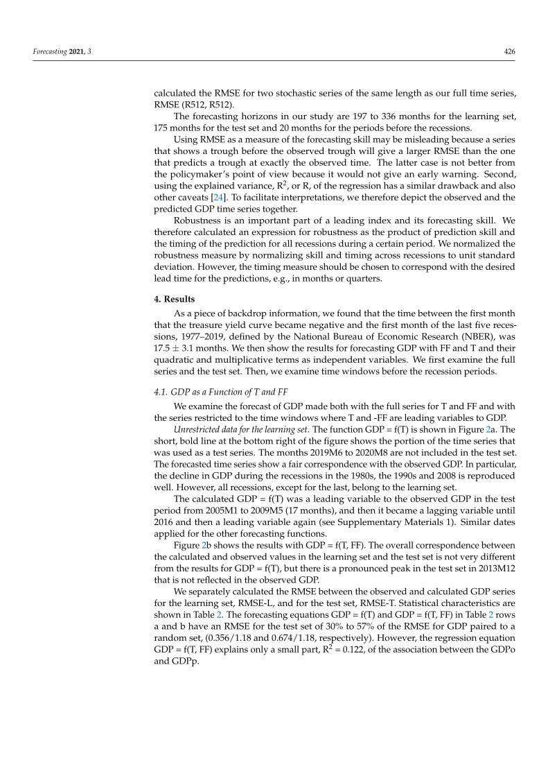
Using RMSE as a measure of the forecasting skill may be misleading because a seriesthat shows a trough before the observed trough will give a larger RMSE than the onethat predicts a trough at exactly the observed time. The latter case is not better fromthe policymaker’s point of view because it would not give an early warning. Second,using the explained variance, R2, or R, of the regression has a similar drawback and alsoother caveats [24]. To facilitate interpretations, we therefore depict the observed and thepredicted GDP time series together.

Robustness is an important part of a leading index and its forecasting skill. Wetherefore calculated an expression for robustness as the product of prediction skill andthe timing of the prediction for all recessions during a certain period. We normalized therobustness measure by normalizing skill and timing across recessions to unit standarddeviation. However, the timing measure should be chosen to correspond with the desiredlead time for the predictions, e.g., in months or quarters.

4. Results

As a piece of backdrop information, we found that the time between the first monththat the treasure yield curve became negative and the first month of the last five reces-sions, 1977–2019, defined by the National Bureau of Economic Research (NBER), was17.5 ± 3.1 months. We then show the results for forecasting GDP with FF and T and theirquadratic and multiplicative terms as independent variables. We first examine the fullseries and the test set. Then, we examine time windows before the recession periods.

4.1. GDP as a Function of T and FF

We examine the forecast of GDP made both with the full series for T and FF and withthe series restricted to the time windows where T and -FF are leading variables to GDP.

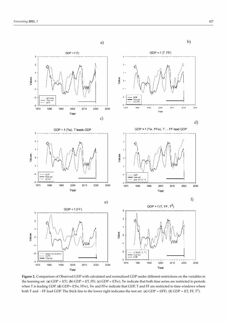
Unrestricted data for the learning set. The function GDP = f(T) is shown in Figure 2a. Theshort, bold line at the bottom right of the figure shows the portion of the time series thatwas used as a test series. The months 2019M6 to 2020M8 are not included in the test set.The forecasted time series show a fair correspondence with the observed GDP. In particular,the decline in GDP during the recessions in the 1980s, the 1990s and 2008 is reproducedwell. However, all recessions, except for the last, belong to the learning set.

The calculated GDP = f(T) was a leading variable to the observed GDP in the testperiod from 2005M1 to 2009M5 (17 months), and then it became a lagging variable until2016 and then a leading variable again (see Supplementary Materials 1). Similar datesapplied for the other forecasting functions.

Figure 2b shows the results with GDP = f(T, FF). The overall correspondence betweenthe calculated and observed values in the learning set and the test set is not very differentfrom the results for GDP = f(T), but there is a pronounced peak in the test set in 2013M12that is not reflected in the observed GDP.

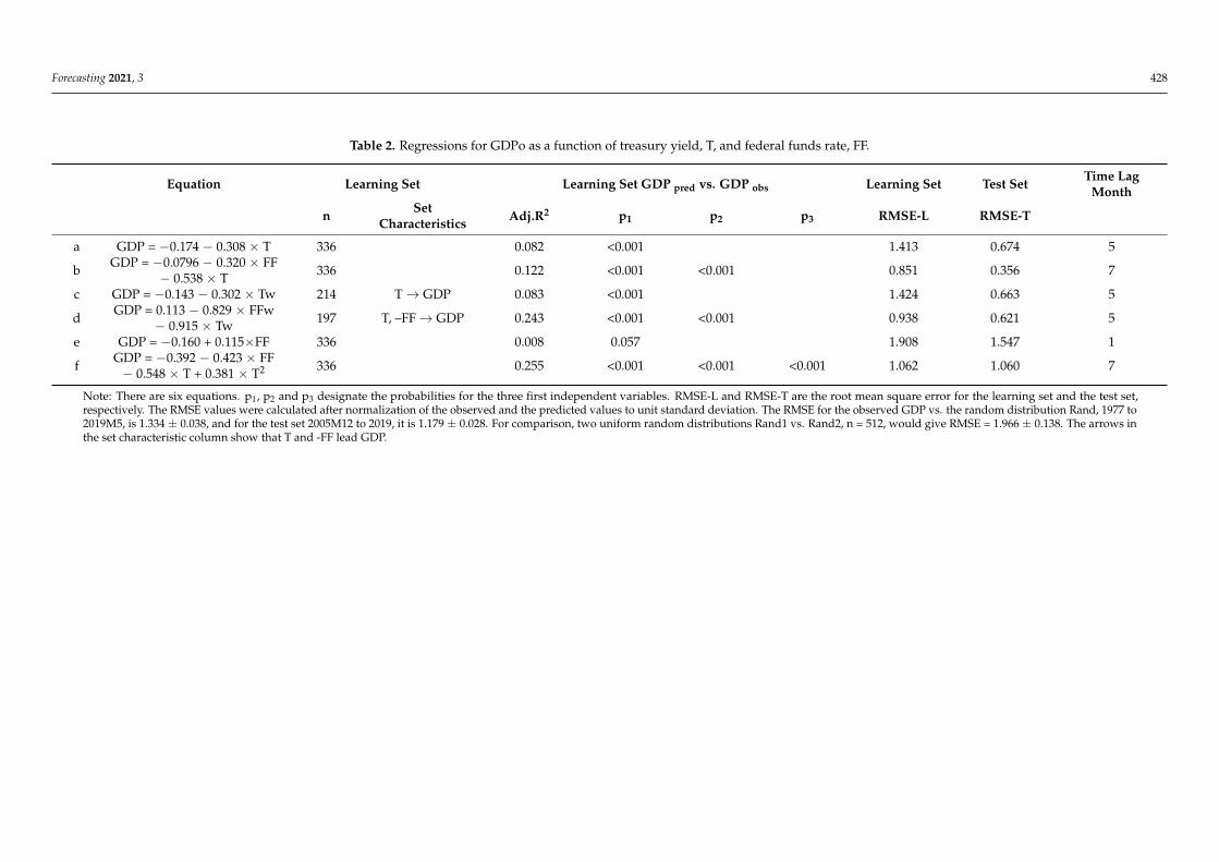
We separately calculated the RMSE between the observed and calculated GDP seriesfor the learning set, RMSE-L, and for the test set, RMSE-T. Statistical characteristics areshown in Table 2. The forecasting equations GDP = f(T) and GDP = f(T, FF) in Table 2 rowsa and b have an RMSE for the test set of 30% to 57% of the RMSE for GDP paired to arandom set, (0.356/1.18 and 0.674/1.18, respectively). However, the regression equationGDP = f(T, FF) explains only a small part, R2 = 0.122, of the association between the GDPoand GDPp.

Forecasting 2021, 3 427Forecasting 2021, 3 FOR PEER REVIEW 7

Figure 2. Comparison of Observed GDP with calculated and normalized GDP under different restrictions on the variables in the learning set. (a) GDP = f(T). (b) GDP = f(T, FF). (c) GDP = f(Tw), Tw indicate that both time series are restricted to periods when T is leading GDP. (d) GDP= f(Tw, FFw), Tw and FFw indicate that GDP, T and FF are restricted to time windows where both T and – FF lead GDP. The thick line to the lower right indicates the test set. (e) GDP = f(FF). (f) GDP = f(T, FF, T2).

The calculated GDP = f(T) was a leading variable to the observed GDP in the test period from 2005M1 to 2009M5 (17 months), and then it became a lagging variable until 2016 and then a leading variable again (see Supplementary Materials 1). Similar dates ap-plied for the other forecasting functions.

Figure 2. Comparison of Observed GDP with calculated and normalized GDP under different restrictions on the variables inthe learning set. (a) GDP = f(T). (b) GDP = f(T, FF). (c) GDP = f(Tw), Tw indicate that both time series are restricted to periodswhen T is leading GDP. (d) GDP= f(Tw, FFw), Tw and FFw indicate that GDP, T and FF are restricted to time windows whereboth T and −FF lead GDP. The thick line to the lower right indicates the test set. (e) GDP = f(FF). (f) GDP = f(T, FF, T2).

Forecasting 2021, 3 428

Table 2. Regressions for GDPo as a function of treasury yield, T, and federal funds rate, FF.

Equation Learning Set Learning Set GDP pred vs. GDP obs Learning Set Test Set Time LagMonth

n SetCharacteristics Adj.R2 p1 p2 p3 RMSE-L RMSE-T

a GDP = −0.174 − 0.308 × T 336 0.082 <0.001 1.413 0.674 5

b GDP = −0.0796 − 0.320 × FF− 0.538 × T 336 0.122 <0.001 <0.001 0.851 0.356 7

c GDP = −0.143 − 0.302 × Tw 214 T→ GDP 0.083 <0.001 1.424 0.663 5

d GDP = 0.113 − 0.829 × FFw− 0.915 × Tw 197 T, –FF→ GDP 0.243 <0.001 <0.001 0.938 0.621 5

e GDP = −0.160 + 0.115×FF 336 0.008 0.057 1.908 1.547 1

f GDP = −0.392 − 0.423 × FF− 0.548 × T + 0.381 × T2 336 0.255 <0.001 <0.001 <0.001 1.062 1.060 7

Note: There are six equations. p1, p2 and p3 designate the probabilities for the three first independent variables. RMSE-L and RMSE-T are the root mean square error for the learning set and the test set,respectively. The RMSE values were calculated after normalization of the observed and the predicted values to unit standard deviation. The RMSE for the observed GDP vs. the random distribution Rand, 1977 to2019M5, is 1.334 ± 0.038, and for the test set 2005M12 to 2019, it is 1.179 ± 0.028. For comparison, two uniform random distributions Rand1 vs. Rand2, n = 512, would give RMSE = 1.966 ± 0.138. The arrows inthe set characteristic column show that T and -FF lead GDP.

Forecasting 2021, 3 429

As all three time series are normalized to unit standard deviation, we can use thecoefficients in front of the independent variables to express the contribution of T and FF tothe prediction of GDP. The T in GDP = f(T, FF) contributes 63% (=0.538/(0.320 + 0.538)) ofthe explanation to the predicted GDP.

Restricted data in the learning set. We restrict the learning set to time windows (w)where T and -FF were leading GDP. The rationale is that the investors that partly determineand partly react to GDP changes may have important prior information. The numericalresults are shown in Table 2 rows c and d. The equation in row d, GDP = f(FFw, Tw), has agreater explained variance with respect to the learning set, 0.243, than GDP = f(FF, T), but itonly forecasts similarly to Equations (a) and (c), that is, it gives an RMSE value around 60%of the test value (0.621/1.18). Except for model GDP = f(FF) in Equation (e), the forecastequations predicted a recession 5 to 7 months before it occurred.

We used all independent variables, T, T2, FF, FF2 and T × FF, as regressors. Onlythe variables T, T2 and FF showed significant contributions after forward and backwardregression. The result is shown in Figure 2f and in Equation (f) in Table 2.

GDP = f(T, F) shows the overall best forecasts for all five recessions, but theGDP = f(T, T2, FF) equation has a similar prediction skill and it predicts the 1990 re-cession better. GDP = f(T) and GDP = f(Tw) make the worst predictions.

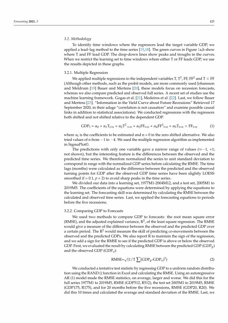
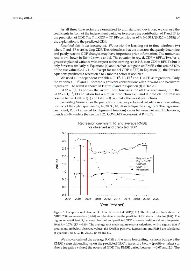
Forecasting horizons. For the prediction curve, we performed calculations at forecastinghorizons 1 through 8 quarters, 12, 16, 20, 30, 40, 50 and 60 quarters, Figure 3. The regressioncoefficient, R, (not adjusted for degrees of freedom) varies between 0.62 and 1.0; however,it ends at 60 quarters (before the 2020 COVID-19 recession), at R = 0.78.

Forecasting 2021, 3 FOR PEER REVIEW 9

Forecasting horizons. For the prediction curve, we performed calculations at forecast-ing horizons 1 through 8 quarters, 12, 16, 20, 30, 40, 50 and 60 quarters, Figure 3. The regression coefficient, R, (not adjusted for degrees of freedom) varies between 0.62 and 1.0; however, it ends at 60 quarters (before the 2020 COVID-19 recession), at R = 0.78.

We also calculated the average RMSE at the same forecasting horizons but gave the RMSE a sign depending upon the predicted GDP’s trajectory below (positive values) or above (negative values) the observed GDP. The RMSE varied between −0.07 and 2.0. The predicted GDP was above and below the observed GDP about 50% of the time, but the cumulative RMSE is positive except at time horizon 30 months.

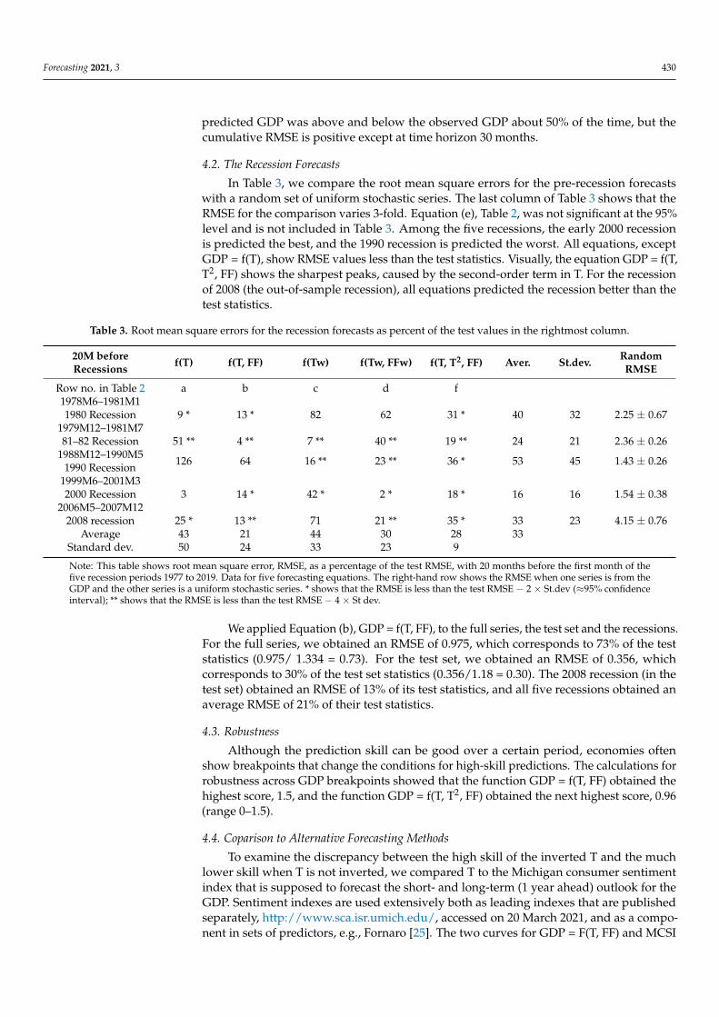
4.2. The Recession Forecasts In Table 3, we compare the root mean square errors for the pre-recession forecasts

with a random set of uniform stochastic series. The last column of Table 3 shows that the RMSE for the comparison varies 3-fold. Equation (e), Table 2, was not significant at the 95% level and is not included in Table 3. Among the five recessions, the early 2000 reces-sion is predicted the best, and the 1990 recession is predicted the worst. All equations, except GDP = f(T), show RMSE values less than the test statistics. Visually, the equation GDP = f(T, T2, FF) shows the sharpest peaks, caused by the second-order term in T. For the recession of 2008 (the out-of-sample recession), all equations predicted the recession better than the test statistics.

Regression coeffisient, R, and average RMSEfor observed and predicted GDP

Year (test set)2004 2006 2008 2010 2012 2014 2016 2018 2020 2022

Valu

es

-0,5

0,0

0,5

1,0

1,5

2,0

2,5

3,0

3,5

Regression, RSign * RMSE GDP obsGDP(FF,T) Recessions

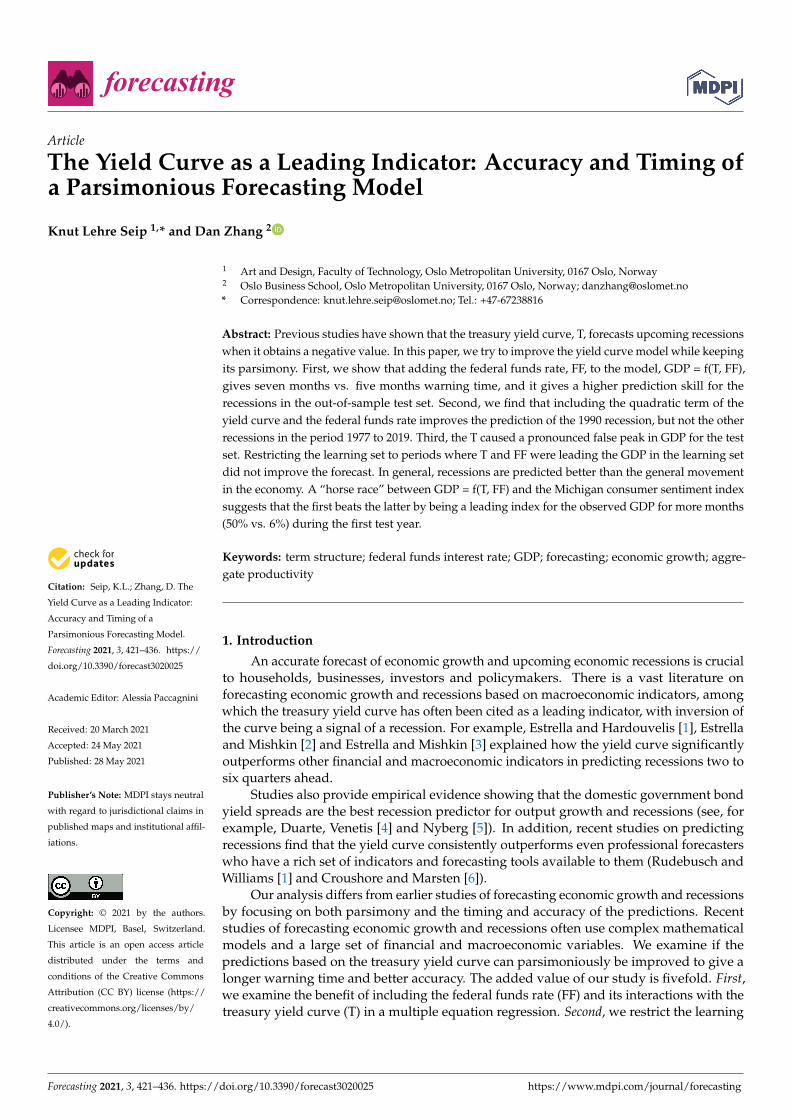
Figure 3. Comparison of observed GDP with predicted GDP(T, FF). The drop-down lines show the NBER 2008 recession date (right) and the date when the predicted GDP starts to decline (left). The regression coefficient, R, between observed and predicted GDP is always positive and ends in quar-ter 60 at R = 0.776, (R2 = 0.60). The average root mean square error is calculated with a sign so that if predictions are below observed values, the RMSE is positive. Regressions and RMSE are calculated at quarters 1 to 8, 12, 16, 20, 30, 40, 50 and 60.

We applied Equation (b), GDP = f(T, FF), to the full series, the test set and the reces-sions. For the full series, we obtained an RMSE of 0.975, which corresponds to 73% of the test statistics (0.975/ 1.334 = 0.73). For the test set, we obtained an RMSE of 0.356, which corresponds to 30% of the test set statistics (0.356/1.18 = 0.30). The 2008 recession (in the test set) obtained an RMSE of 13% of its test statistics, and all five recessions obtained an average RMSE of 21% of their test statistics.

4.3. Robustness

Figure 3. Comparison of observed GDP with predicted GDP(T, FF). The drop-down lines show theNBER 2008 recession date (right) and the date when the predicted GDP starts to decline (left). Theregression coefficient, R, between observed and predicted GDP is always positive and ends in quarter60 at R = 0.776, (R2 = 0.60). The average root mean square error is calculated with a sign so that ifpredictions are below observed values, the RMSE is positive. Regressions and RMSE are calculatedat quarters 1 to 8, 12, 16, 20, 30, 40, 50 and 60.

We also calculated the average RMSE at the same forecasting horizons but gave theRMSE a sign depending upon the predicted GDP’s trajectory below (positive values) orabove (negative values) the observed GDP. The RMSE varied between −0.07 and 2.0. The

Forecasting 2021, 3 430

predicted GDP was above and below the observed GDP about 50% of the time, but thecumulative RMSE is positive except at time horizon 30 months.

4.2. The Recession Forecasts

In Table 3, we compare the root mean square errors for the pre-recession forecastswith a random set of uniform stochastic series. The last column of Table 3 shows that theRMSE for the comparison varies 3-fold. Equation (e), Table 2, was not significant at the 95%level and is not included in Table 3. Among the five recessions, the early 2000 recessionis predicted the best, and the 1990 recession is predicted the worst. All equations, exceptGDP = f(T), show RMSE values less than the test statistics. Visually, the equation GDP = f(T,T2, FF) shows the sharpest peaks, caused by the second-order term in T. For the recessionof 2008 (the out-of-sample recession), all equations predicted the recession better than thetest statistics.

Table 3. Root mean square errors for the recession forecasts as percent of the test values in the rightmost column.

20M beforeRecessions f(T) f(T, FF) f(Tw) f(Tw, FFw) f(T, T2, FF) Aver. St.dev. Random

RMSE

Row no. in Table 2 a b c d f1978M6–1981M11980 Recession 9 * 13 * 82 62 31 * 40 32 2.25 ± 0.67

1979M12–1981M781–82 Recession 51 ** 4 ** 7 ** 40 ** 19 ** 24 21 2.36 ± 0.26

1988M12–1990M51990 Recession 126 64 16 ** 23 ** 36 * 53 45 1.43 ± 0.26

1999M6–2001M32000 Recession 3 14 * 42 * 2 * 18 * 16 16 1.54 ± 0.38

2006M5–2007M122008 recession 25 * 13 ** 71 21 ** 35 * 33 23 4.15 ± 0.76

Average 43 21 44 30 28 33Standard dev. 50 24 33 23 9

Note: This table shows root mean square error, RMSE, as a percentage of the test RMSE, with 20 months before the first month of thefive recession periods 1977 to 2019. Data for five forecasting equations. The right-hand row shows the RMSE when one series is from theGDP and the other series is a uniform stochastic series. * shows that the RMSE is less than the test RMSE − 2 × St.dev (≈95% confidenceinterval); ** shows that the RMSE is less than the test RMSE − 4 × St dev.

We applied Equation (b), GDP = f(T, FF), to the full series, the test set and the recessions.For the full series, we obtained an RMSE of 0.975, which corresponds to 73% of the teststatistics (0.975/ 1.334 = 0.73). For the test set, we obtained an RMSE of 0.356, whichcorresponds to 30% of the test set statistics (0.356/1.18 = 0.30). The 2008 recession (in thetest set) obtained an RMSE of 13% of its test statistics, and all five recessions obtained anaverage RMSE of 21% of their test statistics.

4.3. Robustness

Although the prediction skill can be good over a certain period, economies oftenshow breakpoints that change the conditions for high-skill predictions. The calculations forrobustness across GDP breakpoints showed that the function GDP = f(T, FF) obtained thehighest score, 1.5, and the function GDP = f(T, T2, FF) obtained the next highest score, 0.96(range 0–1.5).

4.4. Coparison to Alternative Forecasting Methods

To examine the discrepancy between the high skill of the inverted T and the muchlower skill when T is not inverted, we compared T to the Michigan consumer sentimentindex that is supposed to forecast the short- and long-term (1 year ahead) outlook for theGDP. Sentiment indexes are used extensively both as leading indexes that are publishedseparately, http://www.sca.isr.umich.edu/, accessed on 20 March 2021, and as a compo-nent in sets of predictors, e.g., Fornaro [25]. The two curves for GDP = F(T, FF) and MCSI

Forecasting 2021, 3 431

are counter-cyclic in 76% of our study period, that is, from 1980 to 2009 and from 2012 to2016. The MCSI is a leading index to GDP 13% of the time during the period 1977 to 2019(Supplementary Materials 2). The inverse relation between the MCSI and the yield curveseems to relax just after the 2008 recessions.

5. Discussion

We used two sets of the independent variables T and FF: first, an unrestricted set, andthen a set restricted to the time windows where the two variables were leading variablesto GDP. Our main argument for restricting the time window is that information is thenavailable in advance.

We first compare the predictions of the six equations that were calibrated on thelearning set to the observed GDP for the full sample period 1977M1 to 2019M5. Then, wecompare predictions to observations for the test set 2005M1 to 2019M5. Last, we comparepredictions to observations for the 20 months prior to the five recessions. Note that it isonly the last 2008 recession that belongs to the test set. We finally discuss how the resultsrelate to the four hypotheses in the introduction.

5.1. Comparison Metrics

We compare our predictions by using the regression coefficient R (and the explainedvariance R2) and by comparing the RMSE of our predictions to stochastic time series.However, the RMSE tends to give a higher (worse) score and the least square (LSQ)methods will give a lower (worse) score the longer the predicted curve is shifted relativeto each other. (Two sine functions that are shifted 1

4 of a common cycle length relative toeach other give a regression coefficient of r = 0.) Still, the predicted and the observed timeseries may be close replicates of each other. Thus, the prediction skill measure dependson the shift between the prediction and observed time series in addition to their cycliccharacteristics. Both R and RMSE metrics are used in the literature, e.g., R (and a pseudo-R)was used by Estrella and Hardouvelis [1] and Fornaro [25], and versions of the RMSE wereused by Gupta et al. [26] and Plakandaras et al. [27].

5.2. Forecasting GDP

The observed and the predicted curves are shown in Figure 2, and the test statisticsfor the full period, the learning period and the test period are shown in Table 2. The teststatistics for the recession periods are shown in Table 3. The regression coefficient, R, waspositive and above the adjusted R2 = 0.426 for all forecasting horizons less than 12 quartersusing GDP = f(FF, T) as the prediction algorithm. Estrella and Hardouvelis [1] found anoptimum adjusted square, R2 = 0.44, for forecasting horizons of six and seven quarters.Thus, the predictions for the period 2005 to 2019 were overall better than those for theperiod 1955 through 1988 studied by Estrella and Hardouvelis [1].

We found that Equation (f): GDP = f(T, T2, FF), and Equation (d): GDP = f(Tw, FFw),gave the largest adjusted explained variance. However, the lowest RMSE values for theout-of-sample forecasts were obtained with Equation (b): GDP = f(T, FF). This equation,and Equation (f), GDP = f(T, T2, FF), gave the longest time period between the forecastedturning point and the recession turning point for the 2008 recession in the test set (7 months).Bauer and Merten [19] reported that the delay between the term spread turning negativeranged between 6 and 24 months. Our initial calculations gave 17.5 ± 3.1 months for thefive last recessions.

Visual inspection of the predicted and the observed GDP series in Figure 2a and eshows that the peak that appeared just after 2010 in the GDP = f(T) graph seems to bedue to the T since it is not present in the GDP = (FF) graph. Thus, the graphs in Figure 2suggest that the optimum forecasting horizon depends on the actual development of theGDP during the test set period and on the forecasting function used, e.g., the false peakcaused by T in 2010.

Forecasting 2021, 3 432

The second-order term in T appears to have four effects on the predicted GDP. Themultiple regression (f) that includes T2 explains a larger proportion of the explainedvariance than the regression (b) without T2. This makes the predicted GDP curves morepeaked. This fits well with the peaks around 2000 and 2008, but not with the 1990 peak andthe recovery period that led up to that peak. It appears to be responsible for an apparentrecovery period in 2009–2010 just after the 2008 recession that did not occur. Finally, theRMSE-T of the out-of-sample predictions was larger than that for all the other alternativeequations, except for Equation (e), with only FF as an argument.

5.3. Recession Periods

To obtain a fuller picture of the forecasting skill of the equations, we also examinedthe four recessions that belong to the learning set. The 1981–1982 and 2000 recessions wereoverall the best predicted (smallest RMSE), and the 1990 recession was predicted the worst,Table 3. The relatively poor prediction during the 1990 recession agrees with the resultsby Estrella [28] and Ang, Plazzesi [16], who found that during the post-1987 period (theVolcker/Greenspan period, McNown and Seip [29]), the predictive power of the yieldspread was diminished probably because of the Volcher strict inflation targeting of themonetary policy.

The RMSE statistics are susceptible to shifts between cyclic series. We used a relativelylarge time window that led up to the recession (20 months) to evaluate the relation betweenthe observed and the predicted values. This would allow for some uncertainty in the timeof the recession prediction. For the latest out-of-sample recession in 2007M12, the timingbetween the observed peak and the predicted peak was, on average, 5 months, rangingfrom 1 to 7 months depending on the equation used.

Visually, the two last recessions in 2000 and 2008 formed the sharpest peaks, that is,the recovery from the previous recession to the 2000 and 2008 recessions was relativelyshort. However, employment growth was relatively slow [30]. The 1990 recession was,in contrast, preceded by a volatile period. The overall best predictor for all recessions isthe GDP = f(T, FF) equation. It gave an overall RMSE of 21% of the test statistics for therecessions. GDP = f(T, T2, FF) came in second place. The only equation that gave a worseresult than the reference statistic was GDP = f(T) for the 1990 recession, Table 3.

5.4. The Hypotheses

We now discuss our four hypotheses.

Hypothesis 1 (H1). The first hypothesis, that T alone would explain most of the variation in thedetrended GDP, was not supported; three other alternatives gave a lower RMSE for the test set andfor the recession forecasts, Tables 2 and 3. Meanwhile, the treasury yield curve T itself appears onlyto have a high predicting skill when it obtains a negative value. Flattening of the T did not reflecta substantial increase in the probability of a near-term recession. A reason may be that the Fed’smonetary policy affects both the FF and the T. Lowering the target FF in anticipation of a comingslowdown may increase the slope of the T [20].

Hypothesis 2 (H2). There is long tradition for adding variables in the predicting algorithm. Oursecond hypothesis, to augment the T with the FF, was supported, but only the second-order termin T enhanced the forecasting skill, and only under certain circumstances. The use of “big datatechniques”, that is, to expose large datasets to data selection techniques, such as PCA or machinelearning techniques, e.g., Stock and Watson [31] and Medeiros et al. [22], respectively, can assistin evaluating variables. The machine learning technique allows modeling of nonlinearities, andthe technique used by Medeiros, et al. [22] computes principal components that include only thevariables that show a high prediction power (the author’s target variable is inflation). A second optionis to use economic insights to evaluate candidate variables. Variables that have proven to robustlycontribute to high prediction skill for inflation are prices, housing prices and employment [22]. Theconference board of the USA uses a composite leading index (CLI) with ten components. Among

Forecasting 2021, 3 433

them is the interest rate spread, T, that has the federal funds rate included, and an average consumerexpectation for business conditions, but not the federal funds rate as an independent component [32].Bauer and Merten [19] showed, using a probit model, that its predictive power is largely unaffectedby including additional variables, e.g., estimates of the natural level of interest or household networth-to-income.

Our prediction function, GDP = f(T, FF), and the MCSI had quite different character-istics with respect to pro- and counter-cyclicity, and the MCSI was a leading index onlyduring 13% of the time in the period it was applied to. We do not have any explanationfor this. In contrast, the German leading indexes ife (lower case letters) and ZEW that arebased on managers’ and economists’ sentiment for changes in IP were leading IP 77–78%of the time (Seip, Yilmaz et al. 2019). A “horse race” between the MCSI and the forecastingfunction GDP = f(T, FF) showed that the MCSI was a leading index to GDP 14% of the testperiod, whereas f(T, FF) was leading 26% of the time. However, for the first year of the testperiod, 2005, f(T, FF) was leading 50% of the time and MCSI 6% of the time.

We provided rationales for introducing interaction and second-order terms for Tand FF in the introduction. We found that the second-order term, T2, could give a betterprediction, but only under certain circumstances (the 1990 recession). The generality ofthose circumstances is not known, but it occurred during the period that is named “TheGreat Moderation”.

Hypothesis 3 (H3). Lead–lag. Lead–lag relations. A variable must be leading the target variableand therefore must be shifted relative to the target to allow measurements of its skill in predictingthe target. Medeiros, Vasconcelos [22] examined four lags (months) for all their candidate variables.However, a process such as hiring or shedding employees may take longer but may still havepredictive power. Our third hypothesis, that restricting the regressions to time windows where Tand -FF were leading variables to GDP would improve predictions, was not supported. For thetest set, the RMSE for the best prediction f(T, FF) increased substantially when restrictions wereapplied, Table 2, Equations (b) and (d). Predictions for the recessions increased the RMSE from 21to 30 percentage points. The reason may be that the portions of the time series where T and -FF werenot leading GDP do not affect the forecasting skill much.

Hypothesis 4 (H4). Recessions and breakpoints in GDP. A crucial question is whether the economyhas evolved so that variables have changed their predictive power. Structural breakpoints in the USeconomy were identified by Perron and Wada [33] and McNown and Seip [29]. Dates during thestudied period are 1975M6, 1979M2, 1983Q4 (the start of the “Great Moderation” period 1983Q4to 1997M2), 1991Q4, 1999Q3 and 2007M4. Our fourth hypothesis, that recession periods wouldbe predicted better than the full time series, was supported (with 21% vs. 73% of the respectiveRMSE). This result is also supported by Hassani et al. [34] studying the 2008 recession during theperiod 2000 to 2010 with the singular spectrum analysis technique. They found that the averageRMSE estimates relative to their benchmark model were for pre-recession (2.11), the recession period(7.11) and the post-recession period (5.60) (their leading series 1–4). Rudebusch [17] suggestedthat the predictive power of the inverted T endures, whereas Schrimpf and Wang [14] showed thatthe predictive power weakened substantially after 1984. Johansson and Meldrum [20] suggestedthat the flattening of the T in the past years is due to a slower expected GDP growth. Seip andMcNown [35] calculated a robustness score based on timing and accuracy and found that the CLI(robustness = 4.0) was, on average, more robust over time than the average working hours (AWH)(robustness = 3.1); however, AWH beat the CLI (robustness = 6.4 to 1.4) during the period 1988:2to 2006. A contrasting result was found by Glosser and Golden [36], who found that AWH hasbeen less associated with the business cycles after the breakpoint in 1979. Generally, economicbreakpoints may alter the conditions for a prediction algorithm to show high prediction skill. For twoGerman sentiment indexes, prediction skill was weakened during periods with abnormal economicstates [15].

Forecasting 2021, 3 434

Finally, we discuss the lead time. The actual FF values become available when the Feddetermines the short-term rates. However, discussions that the Fed may have before FFis actually determined may be available in advance of the actual values [37]. We founda phase shift for T vs. GDP of 15–20 months. This is a little longer than the phase shiftof 12 months used by, for example, Ang et al. [18] in their Fig 2, and the lead times citedby Rudebusch and Williams [38]. We also tried to lag the GDP relative to the FF and theT, but in contrast to Ponka [39] and Wang, Nie [40], lagged variables did not improvethe predictions.

6. Conclusions and Policy Implications

Our study shows that both the treasury yield curve (T) and the federal funds rate(FF) are important indicators for future economy development. To make a prediction for apossible coming recession, one of the forecasting functions, GDP = f(T, FF) or GDP = f(T,T2, FF), should be applied to a learning set. If the forecast predicts a recession, then the realrecession may come at the forecasted recession time plus 5 to 7 months. Our result contrastswith the high prediction skill of the T when it obtains a negative value. However, if the T isapproaching a negative value, but it is not yet known if it will actually reach it, then theuse of forecasting functions such as GDP = f(T, FF) or GDP = f(T, T2, FF) may be beneficial.Furthermore, if there is a choice between the forecasts of a consumer sentiment index orthe GDP = f(T, FF) forecast for the general development of the economy, the latter shouldbe preferred. A second issue, as pointed out by Akerlof and Shiller [41] and Andolfattoand Spewak [42], is that the economic state at the time of a suspected recession may besusceptible to shocks, and the actual recession may, or may not, be triggered by the shock.A question is therefore if investors are better at detecting non-rational behavior than otherdecision-makers, or if they are triggered by a negative T. Second, recessions appear to beeasiest to predict if there has been a long and uninterrupted increase in GDP, such as theincrease before the 2001 recession.

Our study rests on several assumptions that can be questioned, some of which havebeen addressed in the Discussion section. Three notable issues are the use of linear detrend-ing, the effectiveness of using R or RMSE as measures of forecasting skills and the roleof anomalies in the economy for the forecasting skill obtained. This study shows that theforecasting skill differed among recession periods. An area of future research is thereforeto identify, if possible, the economic characteristics of the time windows leading up to eachrecession and the reasons for differences in the prediction skill among recessions.

Supplementary Materials: The following are available online at https://www.mdpi.com/article/10.3390/forecast3020025/s1, Figure S1: Lead–lag (LL) relations for the test set, Figure S2: LL relationsbetween the yield curve and the Michigan sentiment index, US economy.

Author Contributions: Conceptualization, K.L.S. and D.Z.; methodology, K.L.S.; software, K.L.S.;validation, K.L.S. and D.Z.; formal analysis, K.L.S.; investigation, K.L.S. and D.Z.; resources, K.L.S.and D.Z.; data curation, K.L.S. and D.Z.; writing—original draft preparation, K.L.S.; writing—reviewand editing, K.L.S. and D.Z.; visualization, K.L.S.; supervision, D.Z.; project administration, K.L.S.;funding acquisition, K.L.S. and D.Z. All authors have read and agreed to the published version ofthe manuscript.

Funding: This research was funded by Oslo Metropolitan University.

Informed Consent Statement: Not applicable for studies not involving humans.

Data Availability Statement: All data are available from the first author.

Conflicts of Interest: The authors declare no conflict of interest.

References1. Estrella, A.; Hardouvelis, G.A. The Term Structure as a Predictor of Real Economic Activity. J. Financ. 1991, 46, 555–576. [CrossRef]2. Estrella, A.; Mishkin, F.S. The Yield Curve as a Predictor of U.S. Recessions. Curr. Issues Econ. Financ. 1996, 2, 27. [CrossRef]

Forecasting 2021, 3 435

3. Estrella, A.; Mishkin, F.S. Predicting U.S. Recessions: Financial Variables as Leading Indicators. Rev. Econ. Stat. 1998, 80, 45–61.[CrossRef]

4. Duarte, A.; Venetis, I.A.; Paya, I. Predicting real growth and the probability of recession in the Euro area using the yield spread.Int. J. Forecast. 2005, 21, 261–277. [CrossRef]

5. Nyberg, H. Dynamic probit models and financial variables in recession forecasting. J. Forecast. 2010, 29, 215–230. [CrossRef]6. Croushore, D.; Marsten, K. Reassessing the Relative Power of the Yield Spread in Forecasting Recessions. J. Appl. Econ. 2015, 31,

1183–1191. [CrossRef]7. Chauvet, M.; Potter, S. Forecasting recessions using the yield curve. J. Forecast. 2005, 24, 77–103. [CrossRef]8. Lahiri, K.; Monokroussos, G.; Zhao, Y. The yield spread puzzle and the information content of SPF forecasts. Econ. Lett. 2013, 118,

219–221. [CrossRef]9. Yang, P.R. Using the yield curve to forecast economic growth. J. Forecast. 2020, 39, 1057–1080. [CrossRef]10. Galbraith, J.W.; Tkacz, G. Testing for asymmetry in the link between the yield spread and output in the G-7 countries. J. Int.

Money Financ. 2000, 19, 657–672. [CrossRef]11. Venetis, I.A.; Paya, I.; Peel, D.A. Re-examination of the predictability of economic activity using the yield spread: A nonlinear

approach. Int. Rev. Econ. Financ. 2003, 12, 187–206. [CrossRef]12. Estrella, A.; Rodrigues, A.P.; Schich, S. How Stable is the Predictive Power of the Yield Curve? Evidence from Germany and the

United States. Rev. Econ. Stat. 2003, 85, 629–644. [CrossRef]13. Giacomini, R.; Rossi, B. How Stable is the Forecasting Performance of the Yield Curve for Output Growth? Oxf. Bull. Econ. Stat.

2006, 68, 783–795. [CrossRef]14. Schrimpf, A.; Wang, Q. A reappraisal of the leading indicator properties of the yield curve under structural instability. Int. J.

Forecast. 2010, 26, 836–857. [CrossRef]15. Seip, K.L.; Yilmaz, Y.; Schröder, M. Seip Comparing Sentiment- and Behavioral-Based Leading Indexes for Industrial Production:

When Does Each Fail? Economies 2019, 7, 104. [CrossRef]16. Ang, A.; Piazzesi, M.; Wei, M. What does the yield curve tell us about GDP growth? J. Econ. 2006, 131, 359–403. [CrossRef]17. Sugihara, G.; May, R.; Ye, H.; Hsieh, C.-H.; Deyle, E.; Fogarty, M.; Munch, S. Detecting Causality in Complex Ecosystems. Science

2012, 338, 496–500. [CrossRef]18. Seip, K.L.; McNown, R. The timing and accuracy of leading and lagging business cycle indicators: A new approach. Int. J. Forecast.

2007, 23, 277–287. [CrossRef]19. Johansson, P.; System, B.O.G.O.T.F.R.; Meldrum, A. Predicting Recession Probabilities Using the Slope of the Yield Curve. FEDS

Notes 2018, 2018, 1–2. [CrossRef]20. Bauer, M.D.; Merten, T.M. Economic Forecasts with the Yield Curve. FRBSF Econ. Lett. 2018, 7, 1–5.21. Gogas, P.; Papadimitriou, T.; Matthaiou, M.; Chrysanthidou, E. Yield Curve and Recession Forecasting in a Machine Learning

Framework. Comput. Econ. 2014, 45, 635–645. [CrossRef]22. Medeiros, M.C.; Vasconcelos, G.F.; Veiga, Á.; Zilberman, E. Forecasting Inflation in a Data-Rich Environment: The Benefits of

Machine Learning Methods. J. Bus. Econ. Stat. 2021, 39, 98–119. [CrossRef]23. Bauer, M.D.; Mertens, T.M. Information in the Yield Curve about Future Recessions. FRBSF Econ. Lett. 2018, 20, 1–5.24. Pyper, B.J.; Peterman, R.M. Comparison of methods to account for autocorrelation in correlation analyses of fish data. Can. J. Fish.

Aquat. Sci. 1998, 55, 2710. [CrossRef]25. Fornaro, P. Forecasting US Recessions with a Large Set of Predictors. J. Forecast. 2016, 35, 477–492. [CrossRef]26. Gupta, R.; Olson, E.; Wohar, M.E. Forecasting key US macroeconomic variables with a factor-augmented Qual VAR. J. Forecast.

2017, 36, 640–650. [CrossRef]27. Plakandaras, V.; Gogas, P.; Papadimitriou, T.; Gupta, R. The Informational Content of the Term Spread in Forecasting the US

Inflation Rate: A Nonlinear Approach. J. Forecast. 2016, 36, 109–121. [CrossRef]28. Estrella, A. Why Does the Yield Curve Predict Output and Inflation? Econ. J. 2005, 115, 722–744. [CrossRef]29. McNown, R.; Seip, K.L. Periods and structural breaks in US economic history 1959–2007: A data driven identification. J. Policy

Model. 2011, 33, 169–182. [CrossRef]30. Krugman, P. A Post-Post-Modern Slump. Opinion Columnist 2020. New York Times. Available online: https://messaging-

custom-newsletters.nytimes.com/template/oakv2?campaign_id=116&emc=edit_pk_20200512&instance_id=18415&nl=paul-krugman&productCode=PK&regi_id=57060583&segment_id=27424&te=1&uri=nyt%3A%2F%2Fnewsletter%2F6b27f312-af62-4ac3-b058-87e81a8135a4&user_id=310a4fedd4f63eeafefc9a95de963a96 (accessed on 20 March 2021).

31. Stock, J.H.; Watson, M.W. Forecasting Using Principal Components From a Large Number of Predictors. J. Am. Stat. Assoc. 2002,97, 1167–1179. [CrossRef]

32. The Conference Board. Global Business Cycle Indicators; Retrieved 10 November 2013; The Conference Board of Canada: Ottawa,ON, Canada, 2013.

33. Perron, P.; Wada, T. Let’s take a break: Trends and cycles in US real GDP. J. Monet. Econ. 2009, 56, 749–765. [CrossRef]34. Hassani, H.; Heravi, S.; Brown, G.; Ayoubkhani, D. Forecasting before, during, and after recession with singular spectrum

analysis. J. Appl. Stat. 2013, 40, 2290–2302. [CrossRef]35. Seip, K.L.; McNown, R. Monetary policy and stability during six periods in US economic history: 1959–2008: A novel, nonlinear

monetary policy rule. J. Policy Model. 2013, 35, 307–325. [CrossRef]

Forecasting 2021, 3 436

36. Glosser, S.M.; Golden, L. Average work hours as a leading economic variable in US manufacturing industries. Int. J. Forecast.1997, 13, 175–195. [CrossRef]

37. Kliesen, K.L.; Levine, B.; Waller, C.J. Gauging Market Responses to Monetary Policy Communication. Review 2019, 101, 69–91.[CrossRef]

38. Rudebusch, G.D.; Williams, J.C. Forecasting Recessions: The Puzzle of the Enduring Power of the Yield Curve. J. Bus. Econ. Stat.2009, 27, 492–503. [CrossRef]

39. Ponka, H. The Role of Credit in Predicting US Recessions. J. Forecast. 2016, 36, 469–482. [CrossRef]40. Wang, L.; Nie, C.; Wang, S. A New Credit Spread to Predict Economic Activities in China. J. Syst. Sci. Complex. 2019, 32, 1140–1166.

[CrossRef]41. Akerlof, G.A.; Shiller, R.J. Animal Spirits. How Human Psycology Drives the Economy and Why It Matters for Global Capitalism;

Princeton University Press: Princeton, NJ, USA, 2009.42. Andolfatto, D.; Spewak, A. Does the Yield Curve Really Forecast Recession? Econ. Synop. 2018, 2018. [CrossRef]