The Welfare E⁄ects of Intertemporal Price Discrimination · PDF fileThe Welfare E⁄ects of Intertemporal Price Discrimination: An Empirical Analysis of Airline Pricing in U.S....

The Welfare Effects of Intertemporal Price Discrimination:

An Empirical Analysis of Airline Pricing in U.S. Monopoly Markets

John Lazarev∗

Graduate School of Business

Stanford University

This version: June 1, 2012

Abstract

This paper studies how a firm’s ability to price discriminate over time affects production,

product quality, and product allocation among consumers. The theoretical model has forward-

looking heterogeneous consumers who face a monopoly firm. The firm can affect the quality

and quantity of the goods sold each period. I show that the welfare effects of intertemporal

price discrimination are ambiguous. I use this model to study the time paths of prices for

airline tickets offered on monopoly routes in the U.S. Using estimates of the model’s demand

and cost parameters, I compare the welfare travelers receive under the current system to several

alternative systems, including one in which free resale of airline tickets is allowed. I find that

free resale of airline tickets would increase the average price of tickets bought by leisure travelers

by 54% and decrease the number of tickets they buy by 10%. Their consumer surplus would

decrease by only 16% due to a more effi cient allocation of seats and the opportunity to sell a

ticket on a secondary market.

∗I thank Lanier Benkard and Peter Reiss for their invaluable guidance and advice. I am grateful to Tim Armstrong,Jeremy Bulow, Liran Einav, Alex Frankel, Ben Golub, Michael Harrison, Jakub Kastl, Jon Levin, Trevor Martin,Michael Ostrovsky, Mar Reguant, Andrzej Skrzypacz, Alan Sorensen, Bob Wilson, Ali Yurukoglu and participantsof the Stanford Structural IO lunch seminar for helpful comments and discussions. All remaining errors are my own.Correspondence: [email protected]

1 Introduction

This paper estimates the welfare effects of intertemporal price discrimination using new data on

the time paths of prices from the U.S. airline industry. Who wins and who loses as a result of

this intertemporal price discrimination is an important policy question because ticket resale among

consumers is explicitly prohibited in the U.S., ostensibly for security reasons. Some airlines do

allow consumers to "sell" their tickets back to them, but they also impose fees that can make

the original ticket worthless. Just what motivates these practices is a matter of public debate.1

Economic theory suggests that secondary markets are desirable because they facilitate more effi cient

reallocations of goods. Yet the existence of resale markets also would frustrate airlines’ability to

price discriminate over time, which could potentially decrease overall social welfare.

Theoretically, the welfare effects of price discrimination are ambiguous (Robinson, 1933). I

focus on three channels through which price discrimination can affect social welfare. First, price

discrimination changes the quantity of output sold as some buyers face higher prices and buy less,

while other buyers face lower prices and buy more.2 Second, price discrimination can affect the

quality of the product (Mussa and Rosen, 1978). For instance, a firm may deliberately degrade the

quality of a lower-priced product to keep people willing to pay a higher price from switching to the

lower-priced product (Deneckere and McAfee, 1996). Finally, price discrimination can result in a

misallocation of products among buyers. Since consumers potentially face different prices, it is not

necessarily true that the customers willing to pay the most for the product will end up buying it.

Empirically, we know little about the costs and benefits of intertemporal price discrimination.3

There are several reasons why there has been little work on this problem. First, there is a lack

of available data. In the airline industry, price and quantity data that are necessary to estimate

demand have been available to researchers only at the quarterly level. Such data do not allow one

to separate intertemporal discrimination for a given departure date from variation due to different

days of departure. McAfee and te Velde (2007) used a sample of price paths but they did not have

1Consumer advocates speak out against these inflexible policies and question the legality of such practices. If youbuy a ticket, they argue, it’s your property and you should be able to use it any way you want, including giving it toa friend or selling it to a third party. For examples see Bly (2001), Curtis (2007), and Elliot(2011).

2An increase in total output is a necessary condition for welfare improvement with third-degree price discriminationby a monopolist. Schmalensee (1981), Varian (1985), Schwartz (1990), Aguirre et al (2010), and others have analyzedthese welfare effects in varying degrees of generality.

3Exceptions include Hendel and Nevo (2011) and Nair (2007).

2

access to the corresponding quantities. I solve this problem by merging daily price data collected

from the web with quarterly quantity data using a structural model.

A second impediment to studying intertemporal price discrimination is that a structural model

of dynamic oligopoly with intertemporal price discrimination would necessarily be very complicated.

Among other diffi culties, one would have to deal with the multiplicity of equilibrium predictions

and account for multimarket contact the presence of which is well documented in the industry (see

e.g. Evans and Kessides (1994)). I avoid these problems by focusing solely on monopoly routes.

Finally, I use institutional details of the way that prices are set in practice in the industry to

simplify the problem even further.

While I do observe the lowest available price on each day prior to departure, I only observe the

quantity of tickets purchased at each price on a quarterly basis. As a result, it would be diffi cult to

estimate demand and cost parameters directly. Instead, I estimate the parameters of consumers’

preferences indirectly, based on a model of optimal fares. In the model, a firm sells a product to

several groups of forward-looking consumers during a finite number of periods. Consumer groups

differ in three ways: what time they arrive in the market, how much they are willing to pay for a

flight, and how certain they are about their travel plans. The firm cannot charge different prices to

different consumer groups but is able to charge different prices in different periods of sale. There is

no aggregate demand uncertainty.4 Under these assumptions, I show that a set of fares with positive

cancellation fees and advance purchase requirements maximizes the firm’s profit. By contrast, the

market-clearing fare without advance purchase requirements or cancellation fees maximizes the

social welfare defined as the sum of the airline’s profit and consumers’surplus.

For each value of the unknown parameters, my model predicts a unique profit-maximizing path

of fares as well as the corresponding quantities of tickets sold. I match these predictions with data

collected from 76 U.S. monopoly routes. For every departure date in three quarters, I recorded

all public fares published by airlines for six weeks prior to departure. Since quantity data are not

publicly available, I use the model of optimal fares to predict quantities sold at each price level in

each period. I then aggregate these predictions to the quarterly level and match them to data from

4Aggregate demand uncertainty is another reason why an airline facing capacity constraints may benefit fromvarying its prices over time (Gale and Holmes, 1993, Dana 1999). Puller et al (2009) found only modest support forthe scarcity pricing theories in the ticket transaction data, while price discrimination explained much of the variationin ticket pricing.

3

the well-known quarterly sample of airline tickets. To estimate demand and cost parameters, I use

a two-step generalized method of moments based on restrictions for daily prices, monthly quantities

and the quarterly distribution of tickets derived from the model of optimal fares.

For markets in my data sample, the estimates suggest that, on average, 76% of passengers travel

for leisure purposes. A significant share of leisure travelers start searching for a ticket at least six

weeks prior to departure. By contrast, 83% of business travelers begin their search in the last week.

Business travelers are willing to pay up to six times more for a seat and they are significantly less

price-elastic. Business travelers tend to avoid tickets with a cancellation fee as the probability that

they have to cancel a ticket is higher.

These estimates allow me to assess the welfare effects of intertemporal price discrimination.

Compared to an ideal allocation that maximizes social welfare, the profit-maximizing allocation

results in a 21% loss of the total gains from trade. To understand to what extent intertemporal

price discrimination contributes to this loss, I use the estimates to calculate the equilibrium sets of

fares for three alternative designs of the market.

The first scenario assesses the potential benefits and costs of allowing unrestricted airline ticket

resale.5 I model resale by assuming that there are an unlimited number of price-taking arbitrageurs

who can buy tickets in any period in order to resell them later. Under this assumption, the profit-

maximizing price path is flat. The welfare effects of a secondary market, however, are ambiguous.

On the one hand, the secondary market increases the quality of tickets and eliminates misallocations

among consumers. On the other hand, the secondary market can —and, for the markets I consider,

does —reduce the total quantity of tickets sold in the primary market. I find that the average price

of tickets bought by leisure travelers would increase from $77 to $118, and the number of tickets

they buy would decrease by 10%. However, business travelers would face an average price decrease

from $382 to $118, with quantity increasing by 49%. The consumer surplus of leisure travelers

would decline by 16%, the consumer surplus of business travelers would increase by almost 100%,

and the airline’s profit would decrease by 28%. Overall, social welfare on the average route would

increase by 12%, even though the total quantity of tickets sold would go down.

In a second scenario, I return to a market without resale and assume that the monopolist is not

5Recent empirical literature on resale and the welfare effects of actual secondary markets includes Leslie andSorensen (2009), Sweeting (2010), Chen et al (2011), Esteban and Shum (2007), Gavazza et al (2011). Ticket resaleis explicitly prohibited in the U.S. airline industry.

4

allowed to alter the quality of tickets by imposing a cancellation fee but can still charge different

prices in different periods. I find that the monopolist would still discriminate over time but the

equilibrium price path would become flatter, which would reduce misallocations of tickets among

consumers. The average ticket price would go up from $137 to $157. Leisure travelers would benefit

due to the increase in the quality of tickets but would lose from the increase in prices. The net effect

on their consumer surplus would be still positive. Overall, social welfare would slightly increase.

Finally, the third scenario compares the welfare properties of intertemporal and third-degree

price discrimination. Third degree price discrimination implies that the airline can identify the

customers’types and is able to set different prices to different types. By varying the price over

time, the airline captures more than 90% of the profit that it would receive if third degree price

discrimination was possible. Surprisingly, the estimates show that some customer groups would

prefer third-degree price discrimination to intertemporal price discrimination. The total social

welfare is also higher under third degree price discrimination.

The paper informs three important empirical literatures. First, it contributes to the empirical

price discrimination literature. Shepard (1991) considered prices of full and self service options at

gas stations. Verboven (1996) studied differences in automobile prices across European countries.

Leslie (2004) quantified the welfare effects of price discrimination in the Broadway theater industry.

Villas-Boas (2009) analyzed wholesale price discrimination in the German coffee market. Second,

it connects to empirical studies of durable goods monopoly. Nair (2007) estimated a model of

intertemporal price discrimination for the market of console video games. Hendel and Nevo (2011)

estimated that intertemporal price discrimination in storable goods markets increases total welfare.

This paper arrives at a different conclusion for airline tickets. Finally, there are several related

papers that analyze price dispersion in the U.S. airline industry (Borenstein and Rose, 1994, Stavins,

2001, Gerardi and Shapiro, 2009). To the best of my knowledge, this is the first paper to emirically

estimate the welfare effects of intertemporal price discrimination in the airline industry.

The rest of the paper proceeds as follows. Section 2 gives background information on airline

pricing. Section 3 presents a model of optimal fares. Section 4 describes the data used in the

analysis. In Section 5, I show how to use the model of optimal fares to infer demand and supply

parameters from the collected data. Section 6 presents the results of estimation. In Section 7, I for-

mally describe the alternative market designs and present the results of counterfactual simulations.

5

Section 8 concludes.

2 Institutional Background

An airline can start selling tickets on a scheduled flight as early as 330 days before departure. At

any given moment, the price of a ticket is determined by the decisions of two airline departments,

the pricing department and the revenue management department. The pricing department moves

first and develops a discrete set of fares that can be used between any two airports served by the

airline. The revenue management department moves second and chooses which of the fares from

this set to offer on a given day.

The pricing department offers fares with different "qualities" to discriminate between leisure

and business travelers. High-quality fares are unrestricted. Low-quality fares come with a set

restrictions such as advance purchase requirements and cancellation fees. To secure cheaper fares,

a traveler typically has to buy a ticket early, usually a few weeks before her departure date. If her

travel plans later change, she may have to pay a substantial cancellation fee, which often could

make the purchased ticket worthless. These restrictions exploit the fact that business travelers are

usually more uncertain about their travel plans than leisure travelers.

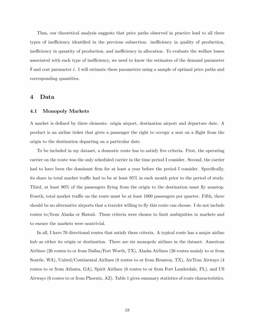
Figure 1 gives a snapshot of all coach-class fares that were published by American Airlines’

pricing department for Dallas —Roswell flights departing on March 1st, 2011, six weeks prior the

departure. Fares with advance purchase requirements include a cancellation fee of $150. Fares

without advance purchase requirements are fully refundable.

The fact that the pricing department has published a fare does not imply that a traveler will be

able to get that fare on the specific flight. The flight needs to have available seats in the booking

class that corresponds to that fare. How many seats to assign to each booking class in each flight

is the primary decision of the revenue management department.

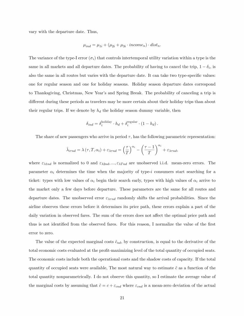
Figure 2 shows the paths of coach-class prices for flights from Dallas, TX to Roswell, NM on

Tuesday, March 1st, 2011. American Airlines is the only carrier that serves this route; there are

three flights available during that day.

The behavior of ticket prices depicted is representative of monopoly markets in my data. There

are three main stylized facts in the data. First, prices increase in discrete jumps. Second, there

6

Figure 1: List of available fares from Dallas, TX to Roswell, NM for 03/11/2011, six weeks beforedeparture

are several distinct times when the lowest price for all flights jumps up simultaneously. As in the

figure, these times typically occur 6, 13 and 20 days before departure. Third, between these jumps,

prices are relatively stable.

This behavior results largely because of the institutional details surrounding the way airlines

set ticket prices. The lowest price of a ticket for a given flight is determined by the lowest fare with

available seats in the corresponding booking class. There are three reasons that the lowest price

of an airline ticket for a given flight may change over time. First, if the number of days before

departure is less than the APR, travelers cannot use that fare to buy a ticket. Less restrictive fares

are usually more expensive, which results in a price increase. If we look at Figure 1 again, we can

see that the first major price increase occurred 20 days before departure: the price went up from

$138 to $154. This was the day when the advance purchase requirement for the two lowest fares

became binding.

Second, the decision of the revenue management department to open or close availability in a

certain booking class may change the lowest price. Eighteen days before departure, the revenue

management department of American Airlines closed booking class S for flight AA 2705 but kept

booking class G open. As a result, the lowest price for this flight went up from $154 to $211.

7

42 35 28 21 14 7 0

138154

211

249

363

463

Number of days before departure

Low

est p

rice

Flight AA2837Flight AA2705Flight AA2775

Figure 2: Example Price Path. Route: Dallas, TX - Roswell, NM. Departure Date: 03/01/11

Finally, the pricing department can add a new fare, as well as update or remove an existing

one. On very competitive routes, airline pricing analysts monitor their competitors very closely:

pricing departments respond to competitor’s price moves very quickly, often responding on the

same day (Talluri and van Ryzin, 2005). On routes with few operating carriers, the set of fares is

usually stable. For example, during the time period depicted on Figure 2, the pricing department

of American Airlines did not update fares for flights from Dallas to Roswell departing on March

1st, 2011. Changes in prices were caused primarily by APR restrictions or the decisions of the

revenue-management department.

8

3 The Model of Optimal Fares

To calculate the welfare effects of intertemporal price discrimination, we need to estimate the

demand system. I estimate the demand system from the supply side. To recover consumers’

preferences (or, to be precise, the airline’s expectations about consumers’preferences), I develop a

model that shows how a set of parameters reflecting travelers’preferences transforms into a path

of profit-maximizing fares.6

A theoretical model that is able to generate the stylized facts listed in Section 2 has to include

the decision problems of both the pricing and revenue-management departments. The solution of

the pricing department’s problem is a finite set of fares that include advance purchase requirements.

To construct an optimal set of such fares, the pricing department has to calculate the value of the

airline’s expected profit for each possible set of fares. This value, in turn, depends on the strategy

of the revenue management department that takes the set of fares as given and updates availability

of each booking class in real time. Another complication comes from the fact that the airline

has to take into account not only direct passengers that travel on a particular route but also

passengers for whom this route is only a part of their trip. I will call them "direct passengers" and

"connecting passengers", respectively. The model is initially formulated for a representative origin

and destination and a representative departure date.

3.1 Airline’s problem

Consider a representative market that is defined by three elements: origin, destination and travel

date. The airline is the only producer in the market. It can offer up to C seats on its flights from

the origin to the destination. It flies both direct and connecting passengers. For direct passengers,

the origin is the initial point of their trip and the destination is the final point of their trip. For

connecting passengers, this flight is only a part of their trip.

The airline is selling tickets during a fixed period of time. Advance purchase requirements divide

this period into T periods of sale. At the beginning of the first period of sale, the airline’s pricing

department sets a menu of fares for this market p = (p1, ..., pT ) and for all markets that connecting

6 I do not consider a more general problem of finding a profit-maximizing mechanism since the mechanism observedin the data is implemented through publicly posted prices. This problem has been studied by Gershkov and Moldovanu(2009), Board and Skrzypacz (2011), and Hoerner and Samuelson (2011), among others.

9

passengers fly pj = (pj1, ..., pjT ). The price pt is the price of the cheapest fare that satisfies the

advance purchase requirement for period of sale t. In the empirical application, advance period

requirements observed define five periods of sale: 21 days and more, from 14 to 20 days, from 7 to

13 days, from 3 to 6 days, and less than 3 days before departure.

The revenue management department at each moment of time decides which of the fares that

satisfy the advance purchase requirements to offer for purchase based on the information ξt. Denote

by Dt (p, ξt) the number of tickets that the airline sells at price pt. Not all passengers that bought

tickets will end up flying. Denote by Qt (p, ξT ) the number of seats that that will be occupied

by passengers who bought tickets at price pt. Both Dt and Qt are the solutions of the revenue

management department’s problem. I will not solve this problem explicitly. Instead, I rely on the

fact that the airline pricing department knows how p affects the number of sold tickets Dt and the

number of occupied seats Qt.

The airline’s revenue comes from selling tickets and collecting cancellation fees. If a traveler

needs to cancel a ticket, she has to pay a cancellation fee f . The fee f ≥ 0 is taken to be exogenous

because in practice U.S. airlines have only one cancellation fee that applies to all domestic routes.

The airline’s operational cost, ϕ (·), depends on the total number of enplaned passengers. Thus,

the airline’s profit takes the following form:

π = R+∑j

Rj − ϕ

Q+∑j

Qj

,where

R =

T∑t=1

(ptQt +min (f , pt)

(Dt − Qt

))revenue from direct passengers,

Rj =T∑t=1

(pjtQjt +min (f, pjt)

(Djt − Qjt

))revenue from connecting passengers,

Q =T∑t=1

Qt the number of seats occupied by direct passengers,

Qj =T∑t=1

Qjt the number of seats occupied connecting passengers from market j.

The pricing department chooses menus of fares p and pj to maximize the expected value of the

profit function subject to the capacity constraint. Formally, the profit maximization problem takes

10

the following form:

maxp,pj

E0π s.t. Q+∑j

Qj ≤ C.

The expectation is taken with respect to all information available at the beginning of the first

period of sale.

I will simplify the problem in three steps. First, the constrained optimization problem can be

written as unconstrained using the method of Lagrange multipliers. Let φ (C) denote the value of

the Lagrange multiplier that corresponds to the capacity constraint. Then the unconstrained profit

function takes the following form:

π = R+∑j

Rj − ϕ

Q+∑j

Qj

− φ (C)Q+∑

j

Qj − C

.The last two components of the profit function represent the economic cost of the airline. The

ϕ (·) term is the operational cost, the φ (·) term is the shadow cost of capacity. Denote by c the

value of the marginal economic cost evaluated at the profit-maximizing level. Then, the solution

of the original profit maximizing problem coincides with the solution of the following problem:

maxp,pj

E0

R+∑j

Rj − c ·

Q+∑j

Qj

.The last problem is separable with respect to p and pj , i.e.

E0

R+∑Rj − c ·

Q+∑j

Qj

= E0 [R− cQ]+∑j

E0[Rj − cQj

].

Thus, if the value of the expected marginal cost c is given, then it is suffi cient to solve the profit-

maximization problem for direct passengers without looking at the fares set for connecting pas-

sengers or knowing the value of the capacity constraint. The value of c can be interpreted in two

ways. First, it reflects the expected marginal revenue of adding an additional unit of capacity to

the market. Second, it is equal to the marginal revenue of flying connecting passengers.

Finally, consider the profit-maximization problem for direct passengers:

maxpE0[R− cQ

]= max

pE0

[T∑t=1

ptQt +min (f, pt)(Dt − Qt

)− cQt

].

11

By law of iterated expectations, we can rewrite the problem as:

maxp

T∑t=1

[(pt − c)Qt +min (f, pt) (Dt −Qt)] , .

where Qt = E0Qt and Dt = E0Dt. The function Dt is the expected number of tickets that will

be sold at price pt if the pricing department offers the menu of fares p and then the revenue

management department behaves optimally given this menu. The function Qt is the corresponding

expected number of occupied seats.

To calculate the welfare effects of intertemporal price discrimination, we need to know how the

quantity of sold tickets and the number of occupied seats respond to changes in the menu of fares

and the cancellation fee. In other words, we need to know the elasticities of demand with respect

to the prices of all available fares and the cancellation fee. Three limitations of the data do not

allow us to estimate these elasticities directly. The number of occupied seats for each fare pt is not

available for each individual flight or departure date. The data include only a 10% random sample

of the quantity data aggregated to the quarterly level. Second, the data do not record tickets that

were sold but later cancelled. Third, it would be hard to find a source of exogenous variation that

comes from the supply-side and would affect the components of the fare menu differently. The form

of the profit function suggests that any variation in the cost function affects the entire menu of

fares in a very specific way. From the pricing department’s point of view, the value of the expected

marginal cost of flying an additional passenger is the same in all periods of sale. Finally, there

is almost no variation in the cancellation fee in the data. Almost all airlines charged $150 in all

domestic markets.

Given these limitations, I follow a different approach. I assume that the market demand defined

by Qt and Dt reflects the optimal decision of strategic consumers whose preferences with respect to

the price and time of purchase depend on a vector of demand parameters θ. The vector of demand

parameters θ determines the level of consumer heterogeneity, their willingness to pay for an airline

ticket, their aversion of the imposed cancellation fee. The airline’s pricing department knows the

value of θ and chooses a menu of fares p to maximize the airline’s profit defined by functions Qt

and Dt that in turn depend on θ and c. Using daily price data and quarterly aggregated quantity

data, I will recover these parameters assuming that the observed prices maximize the airline’s profit

12

for these parameters.

3.2 Demand System and Consumer Welfare

This subsection describes how the vector of demand parameters θ determines the relationship

between the expected quantities of sold tickets Dt, and occupied seats Qt and the menu of offered

fares p. It can be viewed as a micro model of the market demand functions Qt(p; θ)and Dt

(p; θ).

Since these functions by construction represent the expected quantities, the model does not include

any demand uncertainty at the market level.

Types, Arrival and Exit The population of potential direct passengers of size M consists of I

discrete types; types are indexed by i = 1, ..., I. (In the estimation, I assume that I = 2: leisure

and business travelers.) The sizes of different types of potential buyers change over time for three

reasons. First, each period new travelers arrive to the market.7 The mass of new buyers of type

i who arrive at time t is equal to Mit = λit · γi · M , where γi is the weight of each type in the

population and λit is the type-specific arrival rate. Second, those travelers who bought tickets in

previous periods are not interested in purchasing additional ones. Third, each period a fraction of

travelers who arrived in the previous periods learn that they will not be able to fly due to some

contingency, so they cancel the ticket (if purchased) and exit the market. The probability that a

traveler of type i learns that she will not be able to fly is equal to (1− δi) in every period.

Preferences Travelers know their utilities conditional on flying but are uncertain if they are able

to fly. If a traveler ι of type i buys a ticket in period t, she pays the price pt and, conditional on

flying, receives:

uιit ≡ µi + σi (ειit − ειi0) , (1)

where µi is type-i’s mean utility from flying on this route measured in dollar terms, ειit are i.i.d.

Type-1 extreme value terms that shift traveler ι’s utility in each period, and σi is a normalizing

coeffi cient that controls the variance of ειit. The error term ειit reflects idiosyncratic customers’

preferences with respect to the time of purchase. They may reflect customers’tastes with regard to

7Without this assumption, the profit-maximizing monopolist would forgo the opportunity to discriminate overtime (Stokey, 1979). Board (2008) analyzes the profit-maximizing behavior of a durable goods monopolist whenincoming demand varies over time.

13

other characteristics of restricted fares or their idiosyncratic level of uncertainty about their travel

plans. The errors represent the consumer tastes that the airline and the researcher do not observe.

This coeffi cient σi captures the slope of the demand curve and hence the price sensitivity across

the population of type-i travelers: the lower is the coeffi cient, the less sensitive are type-i travelers.

The traveler learns all components of their utilities defined in equation (1) at the beginning of the

period she arrived to the market.8

After purchase, the traveler can cancel a ticket. If she cancels a ticket in period t′, she loses

the price she paid, pt, but may receive a monetary refund if the cancellation fee does not exceed

the price. The refund is equal to max (pt − f , 0). Since the refund does not exceed the price of the

ticket, the traveler will cancel her ticket only if she learns that she is not able to fly. If the traveler

doesn’t fly, her utility is normalized to zero.

Travelers are forward-looking and make purchase decisions to maximize their expected utility.

They face the following tradeoff: if they wait, they will receive more information about their travel

plans but may have to pay a higher prices as the airline could increase prices over time.

Individual demand Consider the utility-maximization problem of a type-i traveler who is in

the market at time τ . She has T − τ periods to buy a ticket. She buys a ticket at time τ only if

it gives a higher utility than buying a ticket in subsequent periods or not buying a ticket at all. If

she buys a ticket in period τ , then her net expected utility is given by:

[δT−τi uiτ +Riτ

]− pτ ,

where Riτ denotes the expected value of the refund:

Riτ =(1− δT−τi

)max (pτ − f , 0) .

Suppose the traveler decides to wait until period τ ′. Then with probability(1− δτ ′−τi

)she

learns about a travel emergency and exits the market. With the remaining probability δτ′−τi she

stays in the market. If she buys a ticket, she receives δT−τ′

i [µi + σi (ειiτ ′ − ειi0)] + Riτ ′ − pτ ′ . In8An alternative assumption would be for travelers to learn a component of ειi before each period of sale.Under

this assumption each customer would compare the current value of the term with its expected future values. Underthe original assumpton each customer would compare this value with its actual future values. Qualitatively we wouldreceive the same results. However, the demand function will not have a closed form solution.

14

this case, her expected utility is equal to

δT−τi [µi + σi (ειiτ ′ − ειi0)] + δτ′−τi (Riτ ′ − pτ ′) .

Thus, the traveler buys a ticket in period τ if the following set of inequalities holds:

δT−τi [µi + σi (ειiτ − ειi0)] +Riτ − pτ > δT−τi [µi + σi (ειiτ ′ − ειi0)] + δτ′−τi (Riτ ′ − pτ ′)

for all τ < τ ′ ≤ T and

δT−τi [µi + σi (ειiτ − ειi0)] +Riτ − pτ > 0.

These inequalities can be rewritten in a more convenient way:

δT−τi µi +Riτ − pτσiδ

T−τi

+ ειiτ >δT−τ

′

i µi +Riτ ′ − pτ ′σiδ

T−τ ′i

+ ειiτ ′ for all τ < τ ′ ≤ T and (2)

δT−τi µi +Riτ − pτσiδ

T−τi

+ ειiτ > ειi0.

Market demand for airline tickets To calculate the firm’s expected demand for tickets, we

need to know the demand of each traveler type as well as the size of each type in a given period.

Denote by sitτ the share of type-i buyers who arrived in period τ and purchase a ticket in period

t conditional on not exiting the market. This share corresponds to the probability that traveler ι

has a realization of ειit, t = τ , ..., T that satisfies inequalities defined in (2). Under the assumption

that ειiτ is extreme value, this share is equal to

sitτ =

exp

(δT−ti µi+Rit−pt

σiδT−ti

)1 +

∑Tk=τ exp

(δT−ki µi+Rik−pk

δT−ki σi

) .Consider the size of type-i buyers who arrived in period τ . By time t, only δt−τi of the initial size

has not exited the market due to a realized emergency. Thus, the total demand of type-i travelers

is equal to:

Dit =

t∑τ=1

sitτδt−τi Miτ ;

the market demand for tickets in period t is given by:

Dt =I∑i=1

Dit.

15

Thus, the vector of demand parameters θ includes the following parameters: shares of each

customer type γi, the mean utilities µi, the price sensitivity σi, the probability of cancellation δi,

the arrival parameters λit.

Number of occupied seats The probability of not cancelling a trip for traveller of type i who

bought a ticket in period t by the time of departure is given by δT−ti . Thus the number of occupied

seats is equal to

Q =T∑t=1

Qt, where Qt =I∑i=1

δT−ti Dit.

Welfare For each price path p, we can calculate the sum of utilities for each type of travelers.

Consider the group of type-i travelers who arrived at time τ and define the average aggregate utility

of this group by viτ (p). Then,

viτ (p) =

∫ιmaxτ≤τ ′≤T

{δT−τi [µi + σi (ειiτ ′ − ειi0)] + δτ

′−τi (Riτ ′ − pτ ′) , 0

}dι.

Integrating with respect to the extreme value distribution, we get:

viτ (p) = δT−τi σi log

(1 +

T∑t=τ

exp

(δT−ti µi +Riτ − pτ

δT−ti σi

)).

Then, the total sum of traveler’s utilities equals:

V (p) =

I∑i=1

T∑τ=1

viτ (p) Miτ .

Define social welfare as the sum of travelers’ex-post utilities and the airline’s profit. The supply

and allocation of seats among travelers are effi cient if they maximize social welfare. A price path

p is called effi cient if it induces effi cient supply and allocation of seats. By the First Welfare

Theorem, the allocation of seats will be effi cient only if all consumers take the same prices into

account. If it is not the case, then there could be two customers who would be willing to trade

with each other right before departure. The reason why the customer who wants to buy the ticket

now didn’t buy it before was his higher probability of cancellation. Therefore, there is always some

positive probability that the ex-post allocation is not effi cient, therefore any price path with a

positive cancellation fee is not effi cient.

Thus, there are three conditions for effi cient supply and allocation of seats. First, the price path

16

has to be flat. Second, it has to equal to the value of the marginal costs c. Third, the cancellation

fee has to be zero. If the cancellation fee is positive, then the expected value of the refund is

different for customers of different types. This fact implies that even thought the airline offers the

same menu of fares to all customers, the effective price of a fare is different for different customer

types.

These conditions reveals two impediments to effi cient supply and allocation of seats: market

power and dynamic pricing. First, if the price exceeds marginal cost, then the number of seats

sold by the airline is lower than the socially effi cient level. As a result, social welfare is lower

than its maximum level due to ineffi ciency in the quantity of production. Second, if the price path

is not flat, then the airline charges different prices in different time periods, which results in a

misallocation of seats among travelers. In this case, social welfare does not achieve its maximum

level due to ineffi ciency in allocation. A positive cancellation fee makes a ticket less attractive to

travelers. For this reason, I refer to it as a measure of ticket quality. A positive cancellation fee thus

implies ineffi ciency in the quality of production. Ineffi ciency in quality of production, ineffi ciency

in quantity of production, and ineffi ciency in allocation are the three reasons why a price path may

not induce an effi cient outcome.

3.3 Optimal Price Path

A price path p is called optimal if it maximizes the airline’s profit π (p):

π (p) =T∑t=1

[(pt − c)Qt +min (f, pt) (Dt −Qt)]

Denote by p∗(θ, c)the optimal price path as a function of the demand parameter θ and the cost

parameter c.

Except for the knife-edge case, the optimal price path implies intertemporal price discrimination,

i.e. prices in different periods of sale are different. Furthermore, in practice, airlines often impose

a positive cancellation fee for lower fares. Even though a positive cancellation fee diminishes the

quality for all traveler groups, travelers with a higher probability of cancellation suffer from it more.

If the probability of cancellation is positively correlated with the utility from flying, the fee screens

travelers by their type.

17

Thus, our theoretical analysis suggests that price paths observed in practice lead to all three

types of ineffi ciency identified in the previous subsection: ineffi ciency in quality of production,

ineffi ciency in quantity of production, and ineffi ciency in allocation. To evaluate the welfare losses

associated with each type of ineffi ciency, we need to know the estimates of the demand parameter

θ and cost parameter c. I will estimate these parameters using a sample of optimal price paths and

corresponding quantities.

4 Data

4.1 Monopoly Markets

A market is defined by three elements: origin airport, destination airport and departure date. A

product is an airline ticket that gives a passenger the right to occupy a seat on a flight from the

origin to the destination departing on a particular date.

To be included in my dataset, a domestic route has to satisfy five criteria. First, the operating

carrier on the route was the only scheduled carrier in the time period I consider. Second, the carrier

had to have been the dominant firm for at least a year before the period I consider. Specifically,

its share in total market traffi c had to be at least 95% in each month prior to the period of study.

Third, at least 90% of the passengers flying from the origin to the destination must fly nonstop.

Fourth, total market traffi c on the route must be at least 1000 passengers per quarter. Fifth, there

should be no alternative airports that a traveler willing to fly this route can choose. I do not include

routes to/from Alaska or Hawaii. These criteria were chosen to limit ambiguities in markets and

to ensure the markets were nontrivial.

In all, I have 76 directional routes that satisfy these criteria. A typical route has a major airline

hub as either its origin or destination. There are six monopoly airlines in the dataset: American

Airlines (26 routes to or from Dallas/Fort Worth, TX), Alaska Airlines (26 routes mainly to or from

Seattle, WA), United/Continental Airlines (8 routes to or from Houston, TX), AirTran Airways (4

routes to or from Atlanta, GA), Spirit Airlines (6 routes to or from Fort Lauderdale, FL), and US

Airways (6 routes to or from Phoenix, AZ). Table 1 gives summary statistics of route characteristics.

18

Table 1: Monopoly routes: summary statisticsmean st.d.

distance 401 213median family income $71,942 $8,432average ticket price $205 $236quarterly traffi c, passengers 16,663 11,854share of major airline, traffi c 0.9953 0.0188share of nonstop passengers 0.9772 0.0255share of connecting passengers 0.6511 0.2616load factor 0.7104 0.0896

4.2 Data Sources

Fares are distributed by the Airline Tariff Publishing Company9 (ATPCO), an organization that

receives fares from all airlines’pricing departments. It publishes North American fares three times

a day on weekdays, and once a day on weekends and holidays10. Until recently, the general public

did not have access to information stored in global distribution systems. Yet a few websites have

provided travelers with recommendations on when is the best time to book a ticket based on this

information. In 2004, travelers received direct access to public fares and booking class availabilities

through several new websites and applications. I recorded fares manually from a website that has

access to global distribution systems subscribed to ATPCO data. This website is widely known

among industry experts and regarded as a reliable and accurate source of public fares11. I recorded

fares that were published six weeks before departure. The period of six weeks is motivated by three

facts. First, few tickets are sold earlier than that period. Second, most travel websites recommend

searching for cheap tickets six to eight weeks before departure. Third, when a pricing department

updates fares it takes into account flights that depart in the next several weeks rather than flights

that depart in the next several days. Thus, I believe that it is reasonable to assume that fares

posted six weeks before departure reflect the optimal decision of pricing departments.

I consider three quarters of departure dates between October 1, 2010 and June 30, 2011. Besides

9Until recently, ATPCO was the only agency distributing fares in North America. In March 2011, SITA, the onlyinternational competitor of ATPCO, received an approval from the US Department of Transport and the CanadianTransportation Agency to distribute data for airlines operating in the region.10On weekdays, the fares are published at 10 am, 1 pm and 8 pm ET. On weekends, the fares are published at 5

pm. In October 2011, ATPCO added a fourth filing feed on weekdays —at 4 pm ET.11 In addition to public fares that are available to any traveler, airlines can offer private fares. Private fares are

discounts or special rates given to important travel agencies, wholesalers, or corporations. Private fares can be soldvia a GDS that requires a special code to access them or as an offl ine paper agreement. In the United States, themajority of sold fares are public.

19

the data on daily fares described above, I use monthly traffi c data from the T-100 Domestic Market

database and the Airline Origin and Destination Survey Databank 1B that contains a 10% random

sample of airline tickets issued in the U.S. within a given quarter. Both datasets are reported to

the U.S. Department of Transportation by air carriers and are freely available to the public. In

the estimation, I control for several route characteristics, which allows me to compare different

markets with each other. These characteristics include route distance, median household income in

the Metropolitan Statistical Areas to which origin and destination airports belong, and population

in the areas. A detailed description of this part of the data is in Appendix B

5 Estimation

5.1 Econometric Specification

My empirical model allows for two types of travelers. I refer to the first type as leisure travelers

(L), and to the second type as business travelers (B). Leisure travelers are highly price sensitive

customers who are ready to book earlier and are more willing to accept ticket restrictions. Business

travelers, on the other hand, are less price sensitive, book their trips later and less likely to accept

restrictions.12 The demand parameters of the model of optimal fares are able to capture these

distinctions.

For a given departure date d = 1, ..., D and a given route n = 1, ..., N , the demand parameters

θnd and the cost parameter cnd determine the optimal price path p∗(θnd, cnd

). These parameters

are known to the airline but unknown to the researcher. The goal of the estimation routine is to

recover θnd and cnd for each date and route from the observed price and quantity data. Given the

limitations of the dataset, I need to reduce the dimension of the unknown parameters. To do this,

I restrict both observed and unobserved variation in the parameters within and across markets.

The shares of each type, γi, are assumed to be the same in all routes and all departure dates.

Type-specific mean utilities from flying, µi, are proportional to the route distance. The propor-

tionality coeffi cient in turn linearly depends on the route median income. These coeffi cients do not

12See, Phillips (2005).

20

vary with the departure date. Thus,

µind = µ1i + (µ2i + µ3i · incomen) · distn.

The variance of the type-I error (σi) that controls intertemporal utility variation within a type is the

same in all markets and all departure dates. The probability of having to cancel the trip, 1− δi, is

also the same in all routes but varies with the departure date. It can take two type-specific values:

one for regular season and one for holiday seasons. Holiday season departure dates correspond

to Thanksgiving, Christmas, New Year’s and Spring Break. The probability of canceling a trip is

different during these periods as travelers may be more certain about their holiday trips than about

their regular trips. If we denote by hd the holiday season dummy variable, then

δind = δholidayi · hd + δregulari · (1− hd) .

The share of new passengers who arrive in period τ , has the following parametric representation:

λiτnd = λ (τ , T, αi) + ελτnd =( τT

)αi−(τ − 1T

)αi+ ελτnd,

where ελ1nd is normalized to 0 and ελ2nd, ..., ελTnd are unobserved i.i.d. mean-zero errors. The

parameter αi determines the time when the majority of type-i consumers start searching for a

ticket: types with low values of αi begin their search early, types with high values of αi arrive to

the market only a few days before departure. These parameters are the same for all routes and

departure dates. The unobserved error ελτnd randomly shifts the arrival probabilities. Since the

airline observes these errors before it determines its price path, these errors explain a part of the

daily variation in observed fares. The sum of the errors does not affect the optimal price path and

thus is not identified from the observed fares. For this reason, I normalize the value of the first

error to zero.

The value of the expected marginal costs cnd, by construction, is equal to the derivative of the

total economic costs evaluated at the profit-maximizing level of the total quantity of occupied seats.

The economic costs include both the operational costs and the shadow costs of capacity. If the total

quantity of occupied seats were available, The most natural way to estimate c as a function of the

total quantity nonparametrically. I do not observe this quantity, so I estimate the average value of

the marginal costs by assuming that c = c+ εcnd where εcnd is a mean-zero deviation of the actual

21

value from its mean. The unobserved error εcnd randomly shifts the opportunity cost of flying a

passenger each day and in each route and also explains a part of the daily variation in observed

fares. It captures factors that affect both the operational costs (such us distance, capacity, etc.),

and the shadow cost of the capacity constraint (the demand of connecting passengers etc.). This

error shifts the entire time path of prices, while ελτnd affects relative levels of the prices in the path.

The total number of potential travelers is different for each route and each departure date. I

denote by Mn the mean number of travelers on route n and assume that the deviations from these

means, the arrival errors ελτnd, and the cost errors εcnd are jointly independent.

Together, we can divide all demand and cost parameters known to the airline into three groups:

estimated coeffi cients θ = (γ, µ, σ, δ, α) , c, and Mn, errors unobserved to the researcher εnd =

(ελnd, εnd), and market specific covariates (hd, xn), where xn denotes route characteristics such as

(distn, incomen). These restrictions allow me to estimate the coeffi cients jointly for all markets in

my sample.

5.2 Moment Restrictions

To estimate the demand parameter θ and cost parameters c, I follow the standard practice of using

both price and quantity data. However, I face the nonstandard complication that these data are

observed with different frequencies: prices are observed daily, quantities are observed quarterly.

Only having quarterly quantity data means that they contain two sources of variation: variation

due to different departure dates and variation due to different purchase dates. I use the model of

optimal fares to distinguish between these two sources of variation.

5.2.1 Daily prices

Define by ptnd the lowest fare satisfying the advance purchase requirement for period of sale t for

route n and departure date d. Since the posted fares should be equal to the optimal fares predicted

by the model, the posted fares should satisfy the system of first order conditions:

G(p, θ)=

∂π(p; θ)

∂p1, ...,

∂π(p; θ)

∂pT

′

.

22

To construct moment restrictions that correspond to the posted prices, we need to invert the system

of equations to derive an expression for the unobserved error term εnd.It turns out that there exists

a unique mapping gP : RT × Rdim(θ) × Rdim(hd) × Rdim(xn) → RT , such that for any θ, it holds

that G (pnd, θ, hd, xn , gP (pnd, θ, hd, xn)) = 0. The proof of this statement follows from the fact that

the system of first order conditions is triangular and linear with respect to the errors. The first

equation includes only εcnd, the second equation includes εcnd and ελ2nd., etc. Thus, we can invert

the system by the substitution method: derive the value of εcnd from the first equation and plug it

into the second one, etc.

Since we assumed that εnd has zero mean, the moment restrictions that correspond to the

observed prices take the following form:

Eεnd = Egp (pnd, θ, hd, xn) = 0.

I use these restrictions as the basis for the first set of sample moment conditions.

5.2.2 Monthly traffi c

The model predicts the expected total number of flying passengers for departure date d and route

n is equal to∑T

t=1Qndt

(pnd, θ

). In the data, we observe the actual number of flying passengers.

Denote by Qtrafficnm the total number of enplaned passengers observed in the data for route n and

month m. Thus, the predicted number of enplaned passengers is equal to

∑d∈month(m)

I∑i=1

T∑t=1

Qndit

(pnd, θ

).

Denote by gM(pnd, θ,Mnm

)=∑

d∈month(m)∑I

i=1

∑Tt=1 δ

T−tid Dit

(pnd, θ

)− Qtrafficnm . This error

comes from the fact that the revenue-management department due to the stochastic nature of the

demand cannot perfectly implement the plan designed by the pricing department. Sometimes it

allocates more seats to a certain class, sometimes less. The goal of the revenue management depart-

ment, however, is to get as close to the target level as possible. Therefore, it is not unreasonable

to assume that the variance of the error is bounded and its expected value is equal to zero. Then,

a moment restriction that corresponds to the observed number of enplaned passengers is given by:

EgM(pnd, θ, Q

trafficnm

)= 0.

23

I use this restriction as to define the second set of sample moment conditions.

5.2.3 Quarterly sample of tickets

Denote by rlnq a ticket issued for market n in quarter q and let p (rlnq) and f (rlnq) denote the

corresponding one-way fare and number of traveling passengers.13 The quarterly ticket data have

several potential sources of measurement error. These data include special fares, frequent flier

fares, military and government fares, etc. To reduce the impact of these special fares, I do the

following. First, I divide the range of possible prices intoB+1 non-overlapping intervals:14 [pb, pb+1],

b = 0, ...., B. For each interval, the model predicts the total number of tickets sold during the

quarter. Hence, we can calculate the model-predicted probability of drawing a ticket from each

interval. Denote by wbnq the probability of drawing a ticket with a price that belongs to interval

[pb, pb+1] for market n in quarter q. This probability equals:

wbnq

(pnd, θ

)=

∑d∈quarter(q)

∑Ii=1

∑Tt=1Qit

(pnd, θ

)· 1 {ptnd ∈ [pb, pb+1]}∑

d∈quarter(q)∑I

i=1

∑Tt=1Qit

(pnd, θ

) ,

Similarly, we can calculate the relative frequency of observing a ticket within a given price

range using the 10% sample of airline tickets. I treat a ticket with multiple passengers as multiple

tickets with one passenger each. If a ticket has a round-trip trip fare, I assume that I observe

two tickets with two equal one-way fares. Finally, I only take into account those intervals for

which the model predicts non-zero probabilities. Denote these frequencies as wbnq and define

gW

(pnd, θ, rnd

)= [w1nq − w1nq, ..., wBnq − wBnq]′.

Assuming that the 10% sample is drawn at random, we can derive the third part of the moment

restriction set from the population moment conditions for each price interval:

EgW(pnd, θ, rnm

)= 0.

To avoid linear dependence of the moment restrictions, I exclude the last interval.

13 I manually removed the taxes to get the published fares. The details are in Appendix B.14 I estimate the model using the following 17 price thresholds: 20, 50, 80, 100, 120, 135, 150, 170, 190, 210, 220,

240, 270, 300, 330, 360, 410.

24

Figure 3: Identification

5.3 Estimation Method and Inference

I use a two-step generalized method of moments. The optimal weighting matrix is estimated

using unweighted moments. For computational purposes, I optimize the objective function for a

monotone transformation of the parameters. This transformation guarantees that the estimates

will be positive and, where necessary, less than one. The standard errors are calculated using the

asymptotic variance matrix for a two-step optimal GMM estimator.

5.4 Identification

Section 5.2 established T moment restrictions based on the daily fare data, one restriction based

on the monthly traffi c data and B restrictions based on the quarterly ticket data. I use these

T +B+1 = 5+17+ 1 = 23 moment conditions to estimate the 15 parameters that define θ and c.

These parameters are identified from the joint distribution of daily optimal prices and quantities

aggregated to the quarterly level. To show identification formally, I would need to prove that the T

moment restrictions can be satisfied only under the true parameter θ0. This fact is rarely possible

to prove without knowing the true distribution of the data.

To gain intuition on what properties of the joint distribution identify each component of the

parameter θ, I performed two simulation exercises using the model of optimal fares. The first

exercise shows how a change in each component of the demand and cost parameter θ affects the

25

profit maximizing vectors of prices and quantities. The second exercise does the opposite. After

changing a component of the price-quantity vector, I find a vector of parameters θ under which the

new price-quantity vector would maximize the airline’s profit. Based on these results, I can provide

an intuitive explanation on how the joint distribution of the data may identify the parameters of

the model. The explanation is, by all means, heuristic as we should keep in mind that whenever we

change one parameter of the model, all components of the profit-maximizing prices and quantities

will necessarily change.

Consider a representative market. The solid line on Figure 3 shows an ideal but yet typical

price path that we observe in the data. For the sake of argument, suppose we also observe the

corresponding quantities of sold tickets for this departure day. These quantities are depicted by

the bar graph on Figure 3. Thus, we know two profit maximizing vectors p = (p1, p2, p3, p4, p5)

and q = (q1, q2, q3, q4, q5). From these vectors, we need to infer the following demand and cost

parameters: a share of each type γ, the mean utilities µi, the within-type heterogeneity parameter

σi, the probability of cancellation δi, the arrival parameters αi, and the cost parameter c.

The behavior of the typical price path can be described as follows. In the first two periods, the

price rises but at a relatively slow level. Then in period 3 or 4, the price jumps up and continues to

increase but, again, with a slower speed. To understand this behavior, consider the tradeoff that

the airline has. Recall that it faces two heterogeneous groups of customers with different marginal

willingness to pay: business travelers are willing to pay more than leisure travelers. Therefore, the

airline can charge a high price and receive a low quantity as most leisure travelers cannot afford

to fly. Alternatively, it can charge a low price but receive a high quantity. The price path suggests

that it should be profit maximizing for the airline to charge a low price in the first periods and

then switch to a high price.

Having this intuition in mind, we can infer that most customers buying early are leisure (type

1) travelers, while customers who are buying later, at a higher price, are business (type 2) travelers.

The exact level of the prices in early periods is determined by the elasticity of leisure travelers, while

the price level in later periods is determined by the elasticity of business travelers. The elasticity

of each group in turn depends on the heterogeneity parameter σi. Similarly, the quantities sold in

early periods reveal information about the mean utility of leisure travelers (µL), while the quantities

sold in later periods depend on the mean utility of business travelers (µB). By comparing the sum

26

of quantities sold in early periods with the total sum of quantities and taking into account the

profit maximizing conditions, we can infer the share of leisure type (γ).

The increase in prices in period 2 comparing to period 1 is determined by the probability of

cancellation. After the first period, customers became more certain about their travel plans since

there are fewer periods of time during which they can learn that they won’t be able to fly. As a

result, they are willing to pay more for the ticket. The airline realizes this change and increases the

price. Since most customers who are buying tickets in the first two periods are leisure travelers,

the change in these two prices identifies the probability of cancellation for leisure travelers (δL).

Similarly, the probability of cancellation for business travelers (δB) is identified from the change

in the last two prices. Further, if no new customers arrived in period 2, the profit-maximizing

quantities in period 1 and 2 would be the same. Customers with a high first-period shock ειi1

would buy in period 2, customers with a high second-period shock ειi2 would buy in the second

period. The picture suggests that it is not the case. The reason why the quantity in period 2 is

higher is the arrival of new customers. For the same reason, quantities in period 4 and 5 are also

different. Thus, the exact difference between the two quantities reveals the value of the arrival

parameter αi.

Finally, the period in which the price jump occurs identifies the value of the cost parameter c.

Intuitively, in the equilibrium, the marginal revenue that the airline receives from business travelers

should be equal to the marginal revenue it receives from leisure travelers and both should be equal

to the value of marginal cost. If the costs are high, then the marginal revenue the airline receives

from leisure travelers has to be higher. Therefore, fewer leisure travelers will be served in the

equilibrium, so the airline has to switch to business travelers sooner. If the costs are low, then the

marginal revenue from leisure travelers has to be low, so the airline will offer the lower price longer.

If the menus of fares are the same for all travel dates within a quarter, we can just divide the

quarterly aggregated quantities by the number of travel dates and apply this intuition directly.

Suppose that the menus of fares are the same except for one travel date, say, Thanksgiving. Then,

this travel date has its own menu of fares, at least one price of which is different from the rest.

We can look at the quantity that are associated with this price and based on this quantity and the

model of optimal fares deduce the quantities for other fares from this menus. After subtracting

these quantities from the aggregated data, we are back in the original setting when the fares are

27

Table 2: Estimates of demand and cost parameters

Leisure Travelers Business TravelersShare of Traveler Type γi 79.71%

(0.20%)20.29%(0.20%)

Mean Utility µi $43.63(1.05)

+

[$7.11(0.01)

+ 0.89(0.05)

incomen

]distn $320.23

(19.35)+

[$27.89(4.95)

+ 2.54(1.54)

incomen

]distn

Price sensitivity σi 0.34(0.007)

2.46(0.06)

Probability of cancellationregular season / holiday season

1− δi 9.95%(0.11%)

/ 0.79%(0.01%)

12.33%(0.13%)

Arrival process parameter αi 0.02(0.09)

7.85(1.82)

Marginal cost c $4.00($12.36)

Note: incomen is in $ 100,000, distn is in 100 miles.

the same for the remaining travel dates. This intuitive explanation suggests that the quantity data

provide us with informative moment conditions despite suffering from aggregation.

6 Results

6.1 Demand and Cost Estimates

Table 2 presents the optimal GMM estimates of the demand and cost parameters. The estimates

suggest that 76% of passengers travel for leisure purposes. Business travelers are willing to pay up

to six times more for a seat and they are less price sensitive. If all fares go up by 1%, the total

demand of leisure travelers goes down by 1.3%, while the total demand of business travelers goes

down by 0.8%. Business travelers tend to avoid tickets with a cancellation fee as the probability

that they have to cancel a ticket is high.

The dynamics of arrival of each traveler type is depicted by dotted lines in Figure 4. A significant

share of leisure travelers start searching for a ticket at least six week prior to departure. By contrast,

83% of business travelers begin their search in the last week. The bar graph in Figure 4 demonstrates

how the number of active buyers changes over time. In the first few periods, the number of active

buyers goes down as travelers buy tickets or learn that they will not be able to fly. The arrival

to the market of new travelers does not counteract this decrease. A week before departure, most

business travelers are estimated to start searching for tickets, so the number of active ticket buyers

goes up.

28

1 2 3 4 50

0.5

1

1.5

2

2.5

3

3.5

Period

77.34%

0%

1.01%

0.01%

0.59%

0.35%

0.42%

3.15%

0.33%

16.77%

All active leisure travelersAll active business travelersNew leisure travelersNew business travelers

Figure 4: Dynamics of active buyers on a route with median income and distance

6.2 Optimal Price Path and Price Elasticities

To put these estimates into perspective, I use the model of optimal fares to calculate the price path

for flights on a route with median characteristics on a non-holiday departure date. Figure 4 shows

this path together with the quantities of tickets purchased in each period by leisure and business

travelers. The figure shows that leisure travelers usually purchase tickets up until seven days before

departure, prior to the moment when most business travelers arrive in the market. When business

travelers arrive, the airline significantly increases the price, trying to extract more surplus from

travelers who are willing to pay more.

Table 3 presents the estimates of price elasticities evaluated at the optimal price path. The

estimates show that in periods 1 and 5 the airline extracts almost the maximum amount of revenue

from travelers as the elasticities are close to one. In both periods, the buyers are almost homogenous.

In period 1, the majority of active buyers are leisure travelers. In period 5, the price is so high that

only business travelers can afford it. By contrast, in periods 3 and 4, the estimates of elasticities

indicate that the maximum revenue is not achieved. As we can see from the quantity estimates in

Figure 5, both groups are buying tickets at the optimal price in these periods.

29

Figure 5: Optimal price path for a route with median distance and income

Table 3: Estimates of price elasticitiesMarket Demand in Period:

Price in Period: t = 1 t = 2 t = 3 t = 4 t = 5

t = 1 −2.634 0.598 0.647 0.562 0.013t = 2 0.549 −6.178 1.596 1.388 0.033t = 3 0.546 1.467 −10.923 2.707 0.072t = 4 0.448 1.207 2.560 −16.538 0.193t = 5 0.034 0.099 0.241 0.695 −2.654

6.3 Welfare Estimates

Compared to the effi cient supply and allocation of seats, the model’s profit-maximizing ticket allo-

cation predicts that travelers and the firm attain 79% of the maximum gains from trade. That the

gains are below 100% is due market power distortions and misallocations due to price discrimina-

tion. Figure 6 shows the distribution of utilities for two groups of travelers who are able to fly on

the day of departure. The first group includes travelers who bought tickets, the second group are

travelers who didn’t buy tickets because of high prices. If the allocation was effi cient, only travelers

who value a ticket more would end up buying it. As we can see from the figure, there is an overlap

in the supports of these two distributions. This fact indicates that the optimal price path leads to

misallocations of seats.

30

0 $100 $200 $300 $400 $5000

0.2

0.4

0.6

0.8

1

Utility conditional on flying

Travelers with a ticketTravelers without a ticket

Figure 6: Distributions of travelers’utilities under the optimal allocation of seats

7 Counterfactual Simulations

In the counterfactual simulations, I consider three alternative market designs that can eliminate

some types of ineffi ciency caused by intertemporal price discrimination. The first scenario allows

costless resale in the presence of market arbitrageurs. Under this assumption, two types of ineffi -

ciency would disappear: quality distortions and misallocations among the consumers. On the other

hand, the third type of ineffi ciency, ineffi ciency in the quantity of production, could increase. In

the second scenario, the airline is allowed to sell only fully refundable tickets. This restriction elim-

inates one type of ineffi ciency, quality distortions. By doing so, it reduces the firm’s ability to price

discriminate, and therefore, decreases allocative ineffi ciency. However, the restriction can increase

ineffi ciency in the quantity of production. The last scenario considers the case of direct price-

discrimination when the airline can perfectly identify customers’types and set prices contingent on

them.

7.1 Costless resale

To study the effects of a potential secondary market, I modify the fare model in the following way.

In addition to travelers and the airline, I assume there exists an unlimited number of arbitrageurs.

In any period, an arbitrageur can buy a ticket from the airline and then sell it to travelers later.

31

The arbitrageurs are price-takers. Their goal is to maximize the difference between the price at

which they buy a ticket and the price they sell a ticket later. Under these assumptions, the optimal

price path has to be flat. To see that, first, note that for any optimal sequence of prices, the

maximum profit of each arbitrageur is zero. Indeed, if an arbitrageur is able to extract some profit

then the airline can repeat her actions and increase its profit, which would violate the condition of

profit-maximization. Since the maximum profit of each arbitrageur is zero, the optimal price path

cannot be increasing. But could it be profitable for the airline to decrease the prices? Only if it

did so without resale. Thus, if the price path without resale is increasing, then the optimal price

path in a market with costless resale is flat.

To calculate the optimal fare in the counterfactual scenario, it is suffi cient to consider the profit

maximization problem assuming that the price path is flat. The share of type-i buyers who arrive

in period τ and purchase a ticket in period t becomes:

sitτ =exp

(µi−pσi

)1 +

∑Tk=τ exp

(µi−pσi

) = exp(µi−pσi

)1 + (T − τ + 1) exp

(µi−pσi

) .This share is the same for all purchase periods t since travelers pay the same price in all periods

and can get a full refund if they have to cancel their tickets. The airline’s profit is equal to:

π(p; θ)= (p− c)

I∑i=1

T∑t=1

δT−ti Dit.

Since the value of the expected marginal costs is identified only at the profit-maximizing level,

we need to make an assumption about its value in the counterfactual scenario. I will make two

alternative assumptions. In the first case, I assume that the expected value of the marginal costs

is flat. This assumption corresponds to an ideal situation in which the airline is able to adjust its

capacity continuously. The value of c will represent the minimum expected value of the average

costs, which is the value of the expected marginal costs evaluated at the minimum effi cient scale.

In the second case, I assume that the graph of the marginal costs is a vertical line, i.e. the airline

cannot adjust their capacity.

In both cases, the welfare effects of ticket resale are unclear because the ability to resell tickets

eliminates the ineffi ciency in quality of production and the flat optimal price eliminates ineffi ciency

in allocation. However, ineffi ciency in the quantity of production may go up since the airline is not

32

Figure 7: Resale (constant marginal costs)

able to price discriminate. To quantify the net effect on social welfare, I use the value of demand

parameters that correspond to a route with median characteristics and a non-holiday travel date.

Figure 7 shows the optimal price path for the first case in which the expected marginal costs are

fixed. If resale were possible, the average price of a ticket bought by leisure travelers would increase

from $77 to $118, while the average price of a ticket purchased by business travelers would decrease

from $318 to $118. The effect on the business traveler is unambiguous: they pay lower price and

buy higher quality product. The effect on the business travelers is theoretically ambiguous. The

price for them increases for two reasons. First, they compete against customers who are willing

to pay more. Second, for a higher quality product they are willing to pay more. The estimates

suggest that the first effect dominates: their consumer welfare goes down by 20%. The number

of seats occupied by them would correspondingly decrease by 10%. The number of seats occupied

by business travelers would go up by 50%. The consumer surplus of business travelers increases

by almost 100%. The airline’s profit decreases by 28%. Overall, social welfare on the average

route increases by 12%. The decrease in the airline’s profit may force the airline to exit from the

market, which will decrease the social welfare to zero. Since the fixed costs of the airline are not

identified without observing any variation in entry-exit behavior, I cannot evaluate how plausible

that outcome may be.

In the first case, the total number of occupied seats goes up. Therefore, to consider the case in

which the airline cannot adjust their capacity, I increased the value of the marginal costs until the

33

Figure 8: Resale (fixed capacity)

number of occupied seats in the counterfactual scenario is equal to its initial level. Figure 8 shows

that qualitatively the welfare effects of intertemporal price discrimination remain the same. The

average price goes up even more, the median price goes down. The airline’s profit decreases even

further. The gains for the business travelers outweighs the losses of leisure travelers and the airline.

In this counterfactual, the ineffi ciency in production is fixed since the total quantity remains the

same. The increase in the social welfare (+6%) comes from elimination ineffi ciency in allocation of

seats caused by intertemporal price discrimination.

7.2 The role of cancellation fee

The cancellation fee has two effects on social welfare. Directly, it affects the quality of production.

Indirectly, it also affects the allocation and supply of tickets as it changes the airline’s ability to price

discriminate over time. A zero cancellation fee achieves the socially optimal level of ticket quality.

On the other hand, the airline loses one of its screening tools, which makes price discrimination

more diffi cult.

With a zero cancellation fee, the expected value of a refund is equal to Riτ =(1− δT−τi

)pτ ,

changing both individual demand functions and the airline’s profit. The share of type-i buyers who

arrived in period τ and purchase a ticket in period t now becomes:

sitτ =exp

(µi−ptσi

)1 +

∑Tk=τ exp

(µi−pkσi

) ,

34

Figure 9: Zero cancellation fee

while the airline’s profit is equal to:

π(p; θ)=

I∑i=1

T∑t=1

δT−ti (pt − c)Dit.

With a zero cancellation fee, the optimal price path becomes flatter. As a result the ineffi ciency

in allocation goes down but ineffi ciency in the quantity of production may go up. The net effect on

social welfare is theoretically ambiguous and depends on the value of demand and cost parameters.

Figure 9 shows the optimal price path on a route with median distance and income departing

on a non-holiday date. With zero cancellation fee, the difference between average prices paid by

business and leisure travelers would go down from $305 to $273. This decrease is mainly caused by

the fact that the average price that leisure travelers pay goes up. The reason why leisure travelers

would be willing to accept higher prices is the better quality of airline tickets. The consumer

surplus of both groups would go up slightly while the airline’s profit would go down. Overall, social

welfare would increase but by a small amount (less than 1%). This result is not too surprising as

the airline does not really need to separate business and leisure travelers as most business travelers

are estimated to arrive in the last periods.

This counterfactual assumes that the time when travelers start searching for the ticket is ex-

ogenous and therefore does not depend on the value of the cancellation fee. The exogeneity of

customers’arrival to the market is the reason why the airline is able to price discriminate. This

assumption, however, may not hold in reality. If there is no cost associated with booking tickets

35

Figure 10: Third degree price discrimination

early, business travelers might start arriving to the market early and book preemptively. This

assumption quickly brings us to the case of costless resale.

7.3 Direct price discrimination

The last counterfactual evaluates the effectiveness of the intertemporal price discrimination strategy.

Suppose the airline can recognize a customer type and charge different prices to different customer

types. Then there will be two price paths: one for business travelers, another for leisure travelers.

The airline will not impose a cancellation fee to separate customers within its type, since there is no

within type variation in the value of the cancellation probability. Therefore, in this counterfactual

I set the cancellation fee to zero. Figure 10 presents the optimal price paths and the corresponding

quantities of sold tickets.

By using intertemporal price discrimination, the airline captures more than 90% of the profit

that it could achieve if type-specific prices were possible. Surprisingly, leisure travelers would

prefer to see type-specific prices. There are two reasons for that. First, the airline does not have

to damage the product by imposing a cancellation fee. Second, leisure travelers do not compete

directly or indirectly with business travelers. As the result, the airline can offer a lower price to

leisure travelers, not fearing to lose the price margin on business travelers. Business travelers lose

from third-degree price discrimination but their loss is smaller than the total gain of leisure travelers

and the airline.

36

8 Conclusion

In this paper, I developed an empirical model of optimal fares and estimated it using new data on

daily ticket prices from domestic monopoly markets. The estimates of demand and cost parameters

for monopoly routes allowed me to quantify the costs and benefits of intertemporal price discrimi-

nation. I found that intertemporal price discrimination results in a lower ticket quality for leisure

travelers, higher prices for business travelers, lower supply of tickets for business travelers, lower

overall supply and misallocations of tickets among travelers. On the other hand, the benefits of

intertemporal price discrimination are lower prices and higher supply for leisure travelers.

I also found that free resale of airline tickets would reduce airlines’ability to price discriminate

over time. As a result, business travelers would win from resale and leisure travelers would lose,

even though the quality of tickets would improve. Overall, the short-run effect of ticket resale on

social welfare is positive. However, since the airline’s profit goes down, it may choose to exit from

the market in the long run. The effect of the cancellation fee on social welfare is small. down, it

may choose to exit the market in the long run. Prices would go up mainly due to an increase in

ticket quality. Finally, I found that intertemporal price discrimination allows the airlines to achieve

more than 90% of the profit that third degree price discrimination would generate.

The study focuses on the set of monopoly markets. There are two potential diffi culties with

generalizing its results to more competitive markets. First, one may worry about the endogeneity

of monopoly markets. As the result, the estimated demand parameters may not be representative

of the entire industry. This is a valid concern unless the difference between monopoly markets

and the rest of the industry is caused by the number of potential preferences, not the difference in

their preferences. The second problem is the impact of competition. While it is very diffi cult to

estimate a dynamic oligopoly model with intertemporal price discrimination, even if we do that, in

the counterfactual scenario, we will have to choose one equilibrium out of many. In particular, we

will have to consider an equilibrium in which a travel agency buys all tickets from the competing

airlines at the beginning of sale and then acts as a monopoly in the secondary market. Whether

this outcome is plausible is a question for future research.

37

References

Aguirre, I., S. Cowan, and J. Vickers (2010): “Monopoly Price Discrimination and DemandCurvature,”The American Economic Review, 100(4), 1601—1615.

Bly, L. (2001): “Web Site for Resale of Air Tickets Shows Promise, but It’s Still a Fledgling,”LosAngeles Times. June 3, 2001.

Board, S. (2008): “Durable Goods Monopoly with Varying Demand,”Review of Economic Stud-ies, 75(2), 391—413.

Board, S., and A. Skrzypacz (2010): “Revenue Management with Forward-Looking Buyers,”Discussion paper, Stanford University.

Borenstein, S., and N. L. Rose (1994): “Competition and Price Dispersion in the U.S. AirlineIndustry,”Journal of Political Economy, 102(4), 653—683.

Chen, J., S. Esteban, and M. Shum (2010): “How much competition is a secondary market?,”Working Paper.

Curtis, W. (2007): “World of Wonders,”The New York Times. December 22, 2007.

Deneckere, R. J., and R. Preston McAfee (1996): “Damaged Goods,”Journal of Economics& Management Strategy, 5(2), 149—174.

Elliot, C. (2011): “Ridiculous or not? Your airline ticket isn’t transferrable,”Consumer advocateChristopher Elliott’s site. March 16, 2011.

Esteban, S., and M. Shum (2007): “Durable-goods oligopoly with secondary markets: the caseof automobiles,”The RAND Journal of Economics, 38(2), 332—354.

Evans, W. N., and I. N. Kessides (1994): “Living by the "Golden Rule": Multimarket Contactin the U.S. Airline Industry,”The Quarterly Journal of Economics, 109(2), pp. 341—366.

Gavazza, A., A. Lizzeri, and N. Roketskiy (2010): “A Quantitative Analysis of the Used CarMarket,”Discussion paper, mimeo, New York University.

Gerardi, K. S., and A. H. Shapiro (2009): “Does Competition Reduce Price Dispersion? NewEvidence from the Airline Industry,”Journal of Political Economy, 117(1), 1—37.

Gershkov, A., and B. Moldovanu (2009): “Dynamic Revenue Maximization with Heteroge-neous Objects: A Mechanism Design Approach,”American Economic Journal: Microeconomics,1(2), 168—198.

Hendel, I., and A. Nevo (2011): “Intertemporal Price Discrimination in Storable Goods Mar-kets,”National Bureau of Economic Research Working Paper Series, No. 16988.

Hoerner, J., and L. Samuelson (2011): “Managing Strategic Buyers,” Journal of PoliticalEconomy, 119(3), 379—425.

Leslie, P. (2004): “Price Discrimination in Broadway Theater,”The RAND Journal of Economics,35(3), 520—541.

38

Leslie, P., and A. Sorensen (2009): “The Welfare Effects of Ticket Resale,”National Bureauof Economic Research Working Paper Series, No. 15476.

McAfee, R. P., and V. te Velde (2007): “Dynamic Pricing in the Airline Industry,”Handbookon Economics and Information Systems, 1.

Mussa, M., and S. Rosen (1978): “Monopoly and product quality,”Journal of Economic Theory,18(2), 301—317.

Nair, H. (2007): “Intertemporal price discrimination with forward-looking consumers: Applicationto the US market for console video-games,”Quantitative Marketing and Economics, 5, 239—292.

Phillips, R. L. (2005): Pricing and revenue optimization. Stanford University Press.

Robinson, J. (1933): “The Economics of Imperfect Competition,”.

Schmalensee, R. (1981): “Output and Welfare Implications of Monopolistic Third-Degree PriceDiscrimination,”The American Economic Review, 71(1), 242—247.

Schwartz, M. (1990): “Third-Degree Price Discrimination and Output: Generalizing a WelfareResult,”The American Economic Review, 80(5), 1259—1262.

Shepard, A. (1991): “Price Discrimination and Retail Configuration,”Journal of Political Econ-omy, 99(1), 30—53.

Stavins, J. (2001): “Price Discrimination in the Airline Market: The Effect of Market Concentra-tion,”The Review of Economics and Statistics, 83(1), 200—202.

Stokey, N. L. (1979): “Intertemporal Price Discrimination,” The Quarterly Journal of Eco-nomics, 93(3), 355 —371.

Sweeting, A. (2010): “Dynamic Pricing Behavior in Perishable Goods Markets: Evidence fromSecondary Markets for Major League Baseball Tickets,”Discussion paper, mimeo.

Talluri, K., and G. Van Ryzin (2005): The theory and practice of revenue management, vol. 68.Springer Verlag.

Varian, H. R. (1985): “Price Discrimination and Social Welfare,”The American Economic Re-view, 75(4), 870—875.

Verboven, F. (1996): “International Price Discrimination in the European Car Market,” TheRAND Journal of Economics, 27(2), 240—268.

Villas-Boas, S. B. (2009): “An empirical investigation of the welfare effects of banning wholesaleprice discrimination,”The RAND Journal of Economics, 40(1), 20—46.

39