The welfare costs of unreliable water service

The Welfare Costs of Unreliable Water Service

Brian Baisa, Lucas Davis, Stephen Salant, and William Wilcox1 University of Michigan

July 2008

Abstract

Throughout the developing world, many water distribution systems are unreliable. As a result, it becomes necessary for each household to store its own water as a hedge against this uncertainty. Since arrivals of water are not synchronized across households, serious distributional inefficiencies arise. We develop a model describing the optimal intertemporal depletion of each household’s private water storage when it is uncertain when water will next arrive to replenish supplies. The model is calibrated using survey data from Mexico City, a city where many households store water in sealed rooftop tanks known as tinacos. The calibrated model is used to evaluate the potential welfare gains that would occur if alternative modes of water provision were implemented. We estimate that most of the potential distributional inefficiencies can be eliminated simply by making the frequency of deliveries the same across households which now face haphazard deliveries. This would require neither costly investments in infrastructure nor price increases.

Key Words: Water Supply Uncertainty, Water Storage, Distributional Inefficiency JEL Codes: D45, O12, O13, Q25, Q28

1 Department of Economics, University of Michigan, 611 Tappan Street, Ann Arbor, MI 48109. Raj Arunachalam, Michael Kremer, Kai-Uwe Kühn, Dick Porter, Rebecca Thornton, three anonymous referees and the editor provided helpful comments. We are especially grateful to Firdaus Jhabvala, water expert and director of the Center for Southeastern Research (Centro de Estudios de Investigación del Sureste) and to Juan Jose Almanza and the other hydraulic engineers at the Insolidum Group (Grupo Insolidum, S.A. de C.V.) for their detailed comments on the paper.

1

1. Introduction

Households in developed countries typically have immediate access to as much

water as they can afford. In the developing world, however, the supply of water is more

haphazard. In many areas, households store up water when it arrives and consume out of

their own inventories until they are re-supplied by truck or other means. In Onitsha,

Nigeria, for example, an elaborate vending system involving tanker trucks supplying

households with storage capabilities is used for those who do not have indoor plumbing.2

In Accra, Ghana, a similar system is used with tanker trucks. Again, water deliveries are

uncertain and households respond by storing water.3 Even among households with piped

water, there is often uncertainty about water availability. In the cities of Bandung and

Jakarta Indonesia, residents store water in tanks called torens in response to unreliable

municipal water service. When their tanks run empty, they pay for water to be delivered

by trucks. In Lima, Peru, 48% of households receive water only during limited hours and

supply interruptions are common.4 In Mexico City, 32% of households report receiving

water during only limited hours and most residents suffer routine supply interruptions.

Indeed, some residents in the southern and southeastern portions of the city receive water

less than once per week.5 In these contexts uncertainty arises due to limited water

availability at the source, mechanical failures, human error, and other factors.

While these systems avoid the large fixed costs required to eliminate the supply

uncertainty, they are not without their own significant costs. If a family in the developed

world can consume as much water as it needs at price p Pesos per thousand liters, then it

will increase its consumption to the point where an additional liter of water would yield

an additional benefit just equal to p Pesos per thousand liters. Since this is true for every

family, there would be no additional gains from inter-family trade. That is, there will

never be a situation where one family would value an additional liter of water more than

another family since every family would value its last drop at p. In the developing world

however, distributional inefficiencies (allocations in which individuals value water

2 Whittington, Dale. Lauria, Donald T. A Study of Water Vending and Willingness to Pay for Water in Onitsha, Nigeria. World Development, Vol. 19, No. 2/3, pp. 179-198, 1991. 3 Porter (1997). 4 Alcázar, Xu and Zuluaga (2002). 5 Haggarty, Brook, and Zuluaga (2002) also report that nine out of sixteen delegations in Mexico City routinely suffer cuts in service.

2

differently at the margin) abound. One family may value water more because the family

has a smaller storage tank or was not re-supplied as recently. One family may be

rationing its water usage tightly while another is allocating its surplus water to frivolous

uses. And yet it would be difficult for the parched family to acquire the water the other

family is wasting. So each system has its own costs.

In many countries, some fraction of the population has access to water at all hours

while the remaining fraction must store water between irregular deliveries. How large

would the benefits be if everyone storing water received it after the same fixed interval?

How large would the distributional gains be if everyone had access to water at all hours?

In this paper, we propose a methodology to answer these questions and show how to

apply it. Answering these questions is difficult for two reasons. At the conceptual level,

we must determine the best consumers can do in the current environment where there is

uncertainty about when water will next arrive. At the empirical level, we must find a way

to calibrate our conceptual model to real-world data despite their limitations. The

methodology we develop is general. For concreteness and illustrative purposes, however,

we focus on its application to Mexico City.

The framework described in the paper applies to households that receive water

infrequently and have the means to store it. Our paper examines the case where municipal

water is delivered by trucks, pipes, or some other form of public distribution.6 In

addition, this framework could be used to model consumption decisions for households

that rely on stored rainwater. We proceed as follows. In section 2, we describe the

conceptual model used to examine the welfare costs of unreliable water service. In

section 3, we discuss properties of the model. In section 4, the model is calibrated with

available data from Mexico City and is used to show the distributional benefits of

alternative regimes of water provision. Section 5 concludes.

6 Our framework also applies to households that access water from a well, pond, river, or other readily available water source. Although typically these households do not face uncertainty about water availability, the high fixed cost of collecting water induces them to store it. See, for example, Kremer, Leino, Miguel and Zwane (2006). Our model describes the optimal depletion of private water storage over time for these households. Our model does not apply to households that are unable to store water because they lack the necessary materials or cannot afford them. These households are unable to smooth water consumption at all, making uncertainty in water provision even more important than in the case we consider here.

3

2. The Model

To understand the best way to deplete stored water when there is re-supply

uncertainty, we formulate a model. This model allows us to quantify the social costs

imposed by water service uncertainty. Unsure of when they will be resupplied,

households use less water than they would if water were always available at the same

price. In addition, to avoid running out of stored water and having to rely on alternative,

more expensive sources, households do not consume at a constant rate but tailor their

consumption to the realized delay since their last resupply of water.

Let U(c) denote household utility from consuming c units of water in a particular

period and assume the utility function is strictly increasing and strictly concave. Let C

denote total household storage capacity. Let p denote the price per liter of water fixed by

the municipality and paid at the time that water is replenished. Let β denote the

exogenous discount factor between periods.

In some specifications, we will assume that households have access to an

emergency water source in which water can be purchased at price p̂ >p. For example,

this could be the price of private water delivered by truck or the implicit price of finding

and boiling one’s own water for consumption. It is assumed that emergency water and

water from storage are perfect substitutes. Since emergency water is more expensive, it

will only be used if a household runs out of stored municipal water. We also assume for

simplicity that there is no fixed cost associated with using emergency consumption and

that it must be paid for at the time of purchase. Since it is always available at a fixed price

( p̂ ), emergency water is never stored.

There is uncertainty about whether or not municipal water will be available in a

particular period. If water is available in that period, the household fills its storage tank

and then consumes as much water from it as desired. If water is not available, the

household must consume water out of its storage tank or from the emergency source.

Denote the conditional probability that water is available during a particular

period i as :1i i nα ≤ ≤ . The parameter iα represents the “hazard rate” – the probability

that there is water service in period i conditional on no water service in the previous i-1

periods. For example, if there has been no water service for six consecutive periods, then

4

7α denotes the probability that there will be water service in the seventh period. We

require 1nα = for some exogenous integer n. This implies that, given that no water has

arrived in the previous n-1 consecutive periods, it is certain that additional water will

arrive in the next period. Whenever water arrives, the stochastic process of arrivals

restarts. In particular, this means that the probability of water service directly following a

period with service is 1α .

For convenience we also define,

1 1γ α= ; 1

1

(1 ) for 2,...,i

jj

i nα−

=

= − =∏i iγ α

as a discrete probability distribution that water service next becomes available in period i,

where i is the ith period following the last arrival. For example, 7γ is the probability that

water service next becomes available on the 7th period after the last arrival.

Households must decide how much water to consume in each period. Let

denote the amount of water the household consumes in a period with water service and

let denote its consumption if there has been no water service for the

previous i-1 periods. We consider the present-value of any contingent consumption

strategy which the consumer would recommence every time water is delivered. From

this, we can derive both the best such strategy and the discounted expected value of

pursuing it indefinitely.

0c

(for 1c i ,...,i = 1)n −

The discounted expected value of any repeated contingent consumption strategy

will be denoted V. We assume that each household begins period zero with a full storage

tank and require each consumer to refill his tank to capacity each time the opportunity to

do so arises. We will discuss the circumstances under which refilling to the full capacity

is optimal and will assume that these prevail. We also assume that, unless emergency

supplies are utilized, each household must consume from its own storage tank and not

directly from source of resupply or from a neighbor.

The present value of any repeated contingent strategy can then be written as:

5

(1) ( )

10 0 0 1 1 11 1

1 0 0 0 0 2 2 20 1

1

1 0

ˆ ˆ( ) [ ( ) ]ˆ( )

( )

ˆ( [ [ ( ) ] ] ),

e e e ee e

jni e e j j

j i i i ij i

U c c pc U c c pcV U c c pc V pc

V p c c

U c c pc p c V

βγ β β γ

β β

γ β β β−

= =

⎛ ⎞+ − + + − += + − + − + ⎜ ⎟⎜ ⎟− +⎝ ⎠

= + − − +∑ ∑

+

ic

where denote consumption of stored water and emergency water, respectively, i

periods since the last resupply.

and eic

Equation (1) has the following interpretation. Emergency water may be acquired and

consumed in any period at price p̂ . Municipal water is re-supplied in the jth period with

probability (for 1,..., )j j nγ = , and in that event the agent receives the discounted utility

of consumption from period 0 through j-1 (net of the present cost of replacing the

cumulative consumption in period j) plus the value of starting with a full tank at j and

continuing to use the contingent strategy forever after. Summing and solving for V, we

obtain:

(2)

1

1 0

1

ˆ{ [ ( ) ] }.

1

jni e e j

j i i ij i

nj

jj

U c c pc p cV

γ β β

γ β

−

= =

=

⎡ ⎤⎛ ⎞+ − −⎢ ⎥⎜ ⎟

⎝ ⎠⎣ ⎦=⎛ ⎞−⎜ ⎟

⎝ ⎠

∑ ∑

∑

i

The numerator of this expression is simply the expected sum of discounted

utilities, net of re-supply charges, in a single round (from one period of resupply to the

next). The denominator, which is independent of , inflates the expected payoff from

one round to obtain the payoff into the infinite future.

ic

If agents are utility-maximizers, they will choose the contingent

consumption strategy to maximize the expected present value (V) subject to

the constraint that the sum of contingent consumptions of water in storage

cannot exceed the capacity (C ) of the storage tank:

6

0 1 1

0 1 1

, ,...,

, ,...,

1

0

* max V

subject to 0,

ne e e

n

c c c

c c c

n

ii

V

C c

−

−

−

=

=

− ≥∑

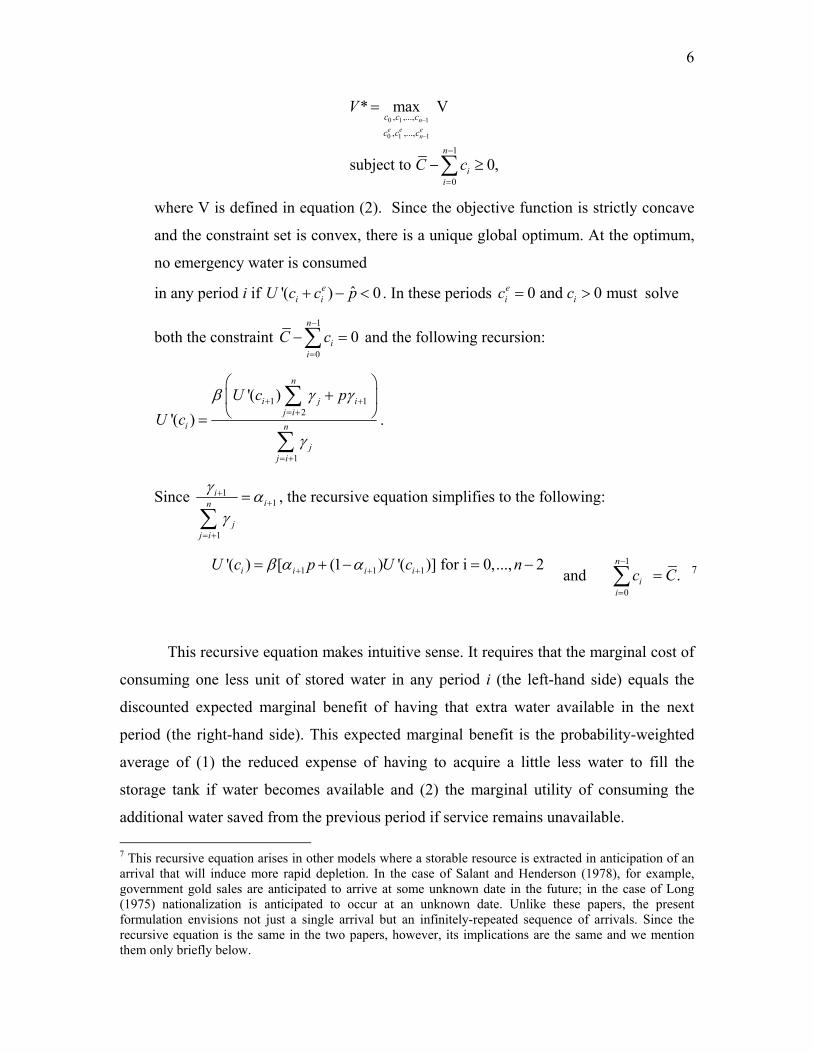
where V is defined in equation (2). Since the objective function is strictly concave

and the constraint set is convex, there is a unique global optimum. At the optimum,

no emergency water is consumed

in any period i if . In these periods solve ˆ'( ) 0ei iU c c p+ − < 0 and 0 must e

i ic c= >

both the constraint 1

0

0n

ii

C c−

=

− =∑ and the following recursion:

1 12

1

'( )'( )

n

i j ij i

i n

jj i

U c pU c

β γ

γ

+ += +

= +

⎛ ⎞+⎜ ⎟

⎝ ⎠=∑

∑

γ.

Since 11

1

iin

jj i

γ αγ

++

= +

=

∑, the recursive equation simplifies to the following:

1 1 1'( ) [ (1 ) '( )] for i 0,..., 2i i i iU c p U c nβ α α+ + += + − = − and

1

0.

n

ii

c C−

=

=∑ 7

This recursive equation makes intuitive sense. It requires that the marginal cost of

consuming one less unit of stored water in any period i (the left-hand side) equals the

discounted expected marginal benefit of having that extra water available in the next

period (the right-hand side). This expected marginal benefit is the probability-weighted

average of (1) the reduced expense of having to acquire a little less water to fill the

storage tank if water becomes available and (2) the marginal utility of consuming the

additional water saved from the previous period if service remains unavailable. 7 This recursive equation arises in other models where a storable resource is extracted in anticipation of an arrival that will induce more rapid depletion. In the case of Salant and Henderson (1978), for example, government gold sales are anticipated to arrive at some unknown date in the future; in the case of Long (1975) nationalization is anticipated to occur at an unknown date. Unlike these papers, the present formulation envisions not just a single arrival but an infinitely-repeated sequence of arrivals. Since the recursive equation is the same in the two papers, however, its implications are the same and we mention them only briefly below.

7

The recursive equation implies that the marginal utility of consumption grows

over time. But since a necessary condition for optimality is that ,

marginal utility cannot exceed the emergency price,

ˆ'( ) 0ei iU c c p+ − ≤

ˆ.p At that point, it is optimal for the

agent to switch to emergency water and U c ˆ'( 0p)ei ic+ − = thereafter until the next

delivery of municipal water. In continuous time, there would be no measurable interval

where both stored water and emergency water were used at the same time. In our

discrete-time formulation, there may be at most one transition period in which water from

both sources is used but only if the marginal utility of consumption in that period is

exactly p̂ .

For any arbitrary level of consumption in period zero, the recursion describes

consumption (contingent on the failure of new supplies to arrive) in all future periods

until the “backstop” price p̂ is reached, after which emergency water will be utilized.

The requirement that the contingent consumptions sum to the initial inventory of water

uniquely determines the initial consumption and hence the whole path.

3. Properties of the Model

3.1 How Periodic but Certain Deliveries Affect Depletion of Stored Water

In the special case where water is certain to arrive in the next period ( 1 1γ = ), no

emergency water is consumed 0( 0ec )= . Under the circumstances prevailing in Mexico

City and elsewhere, a household cannot store even as much water as it would consume in

one day (at the same price) if water was always available. If one is certain of delivery the

next day, it is optimal to consume the entire inventory on the day of delivery 0 =( )c C .

The payoff from doing so collapses to ( ) ,1

U C p CV ββ−

=−

which is strictly increasing in

C since argmax ( )cC U c pcβ< − . Hence, even if water is delivered every day, storage

capacity limits consumption.

If water is sure to arrive on day n (>1) and not before ( ( 1 for 1)n nγ = > ), then for

8

marginal utilities below the emergency price, the recursion requires that

1'( ) '( ) for 0,..., 2.i iU c U c i nβ += = −

)

This “certainty case’’ coincides with the standard

model of an agricultural good where harvests of the same size arrive periodically and

must be stored within the season until the next harvest arrives. The household consumes

stored water so that the discounted value of additional consumption is equalized across

periods. If the household does not discount future payoffs ( 1β = , it is optimal to

consume at the constant rate of /c C= n

)

in each period. The longer the interval between

refills, the smaller is daily consumption. If the household discounts future payoffs ( 1β < ,

it consumes a portion of the initial inventory on the first day ( 0'( ) '( )U c U C pβ> > ) and

successively less in future periods 1( ic c+ )i< so that marginal utility increases by the

factor 1β − (>1). The longer the interval between refills (n), the smaller will be

consumption in each period since the unchanged supplies ( )C have to last longer.8

3.2 How Uncertainty Affects Depletion of Stored Water

If there is some chance that water may arrive before day n, the recursion requires

that marginal utility rise over time by strictly more than the interest factor:

1 11

1 1

'( ) '( ) '( ) '( )'( ) ,(1 ) (1 )i i i i i i

ii i

U c p U c U c U cU c βα αβ α β α β

+ ++

+ +

− −= > =

− −

8 As we will see in the simulations which follow, the introduction of uncertainty always reduces welfare. This result follows unless households discount the future so heavily that they put more weight on a chance early arrival of water than on the painful consequences of a later arrival. While this counterintuitive result never arises in the our application, it might arise in situations where a much longer time scale is involved (for example, Europe's resupplying of early settlements in North America in the past or the resupplying of space missions in the future).

9

where the inequality follows from the assumption that resupply may occur in the next

period 1( i 0)α + > , that marginal utility is monotonically increasing and that storage

capacity is limited and fully utilized 0( '( ) '( ) )iU c U c pβ> > .

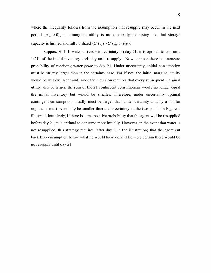
Suppose β=1. If water arrives with certainty on day 21, it is optimal to consume

1/21st of the initial inventory each day until resupply. Now suppose there is a nonzero

probability of receiving water prior to day 21. Under uncertainty, initial consumption

must be strictly larger than in the certainty case. For if not, the initial marginal utility

would be weakly larger and, since the recursion requires that every subsequent marginal

utility also be larger, the sum of the 21 contingent consumptions would no longer equal

the initial inventory but would be smaller. Therefore, under uncertainty optimal

contingent consumption initially must be larger than under certainty and, by a similar

argument, must eventually be smaller than under certainty as the two panels in Figure 1

illustrate. Intuitively, if there is some positive probability that the agent will be resupplied

before day 21, it is optimal to consume more initially. However, in the event that water is

not resupplied, this strategy requires (after day 9 in the illustration) that the agent cut

back his consumption below what he would have done if he were certain there would be

no resupply until day 21.

10

Figure 1: The Effect of Uncertainty on the Optimal Contingent Consumption Path

No Uncertainty Uncertainty

Re-supply Every 21st Day Re-supply May Occur Before 21st Day

In constructing Figure 1-4 we assume a period is one day, resupply on day 21 is

assured (n=21) if it has not occurred before then and that if there is re-supply uncertainty,

components of the alpha vector increase linearly from zero to one over the 21 days. The

household is assumed to have a utility function of the form ( ) ( ) ,U c k c s θ= − where c

represents daily water consumption. The parameter k is a scaling constant, s is some

minimum level of consumption needed to maintain sanitary conditions and θ is a

measure of the curvature of preferences; the three parameters are chosen so that the utility

function is strictly increasing and strictly concave.9

3.3 How Availability of Emergency Water Affects Contingent Consumption

Assume that emergency water is priced low enough that the consumer would

utilize it some time before period n if resupply did not occur. Then, a reduction in the

emergency price must cause the initial marginal utility to be strictly smaller, contingent

9 If the utility function is U(c)=k(c-s)θ it is straightforward to show that U’(c)>0 if kθ>0 and U’’(c)<0 if in addition θ-1<0. We assume the following parameters in our simulations, k=-3194.37, θ=-1.0711, and s=152.8. In addition, we use β=.999813, p=2.86 and p̂ =100 Pesos per 1000 liters. The selection of these parameters is described in Section 4.

11

consumption of municipal water to be larger in each period, and emergency water to be

utilized (in the absence of resupply) at an earlier date. This in turn implies that the

probability that emergency water is used is higher.10

We illustrate these points in Figure 2. A decrease in the emergency price leads to

uniformly larger contingent consumptions. Intuitively, the lower the cost of the

emergency water, the more the agent is willing to risk running out of stored municipal

water by depleting his stored water at a faster rate.

10 For, if on the contrary, instead a reduction in the emergency price caused the initial marginal utility to be weakly larger, then the recursion would imply that every subsequent marginal utility would be weakly larger than before, the strictly smaller emergency price would be reached at an earlier date, and hence the sum of contingent consumptions would be strictly smaller and would no longer match the unchanged initial inventory. So, the marginal utilities must instead be strictly smaller in every period and the contingent consumptions generating them must be larger than before the reduction in the emergency price. But then the water tank must be depleted sooner than before and the probability that emergency water will have to be used will be higher.

12

Figure 2: Optimal Consumption Path By Price of Emergency Water (in Pesos per thousand liters)

3.4 How an Enlarged Storage Capacity Affects Contingent Consumption

The effect of increased storage capacity on optimal contingent consumption can

be deduced in a similar way. An increase in the initial inventory must cause the initial

marginal utility to be strictly smaller, contingent consumption of municipal water to be

larger in each period, and emergency water to be utilized (in the absence of resupply) at a

later date.11 This in turn implies that the probability that emergency water is used is

lower.

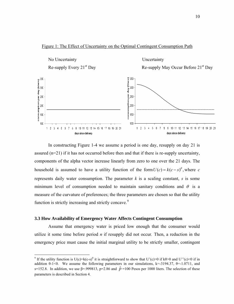
Figure 3 describes the optimal consumption paths and emergency water use for storage

tanks ranging from 500 liters to 3500 liters. As capacity increases, it is optimal to increase

contingent consumption uniformly and to postpone the first use of emergency water.

11 For, if on the contrary, an increase in storage capacity caused the initial marginal utility to be weakly larger, then the recursion would imply that every subsequent marginal utility would be weakly larger than before, the unchanged emergency price would be reached at an earlier date, and hence the sum of contingent consumptions would be strictly smaller and could not equal the enlarged initial inventory.

13

Figure 3: Optimal Consumption Paths By Storage Tank Capacity (in liters)

3.5 Expected Long-Run Consumption

We can also use the model to determine the effect of storage capacity on expected

long-run consumption of municipal and emergency water. Define a “state” as the number

of days that have elapsed since the storage tank was last filled (0, 1,…, n-1). State

transitions are generated by a first-order Markov process. Denote the probability of

transiting in one step from state i to state j as for , 0,..., 1ijp i j n= − . Then,

0 1 1,0 , 1 1for 0,..., 2, 1, and 1 for 1,..., 2. All other transition probabilities are zero. Since this Markov process is regular

i i N i i ip i n p p i nα α+ − + += = − = = − = −

(Grinstead and Snell, 1997), the probability that the system will be in each of the n

possible states after T transitions converges to a limiting distribution asT . One way

to determine this distribution is to note: for

→∞

i =1,...n-1,

14

0 1

0

P(c ) ( ) (1 ). That is, the probability that in the steady state

is consumed equals the probability that in the steady state is consumed andand that there will then be consecutive peri

ii j ij

P c c

ci

α=

= −∏

ods with no re-supply.

1

0 011

Since the states are mutually exclusive and exhaustive,

( )[1 (1 )] 1. From this last equation, ( ) can be deduced

the other 1 probabilities of the stationary dis

n ijj

i

n

P c P c

n

α−

==

+ − =

−

∑∏tribution. This derivation a

establishes that the stationary distribution is unique. Expected daily consum

and, from that,

lso ption

(and its decomposition into consumption of municipal water and emergency water) are

computed with respect to this limiting distribution. In particular, since each household

finds it optimal to consume municipal water for an interval we can determine and then to

switch to emergency water, we can use this limiting probability distribution to compute

separately the expected daily consumption of emergency water and the expected daily

consumption of municipal water in the long-run equilibrium.

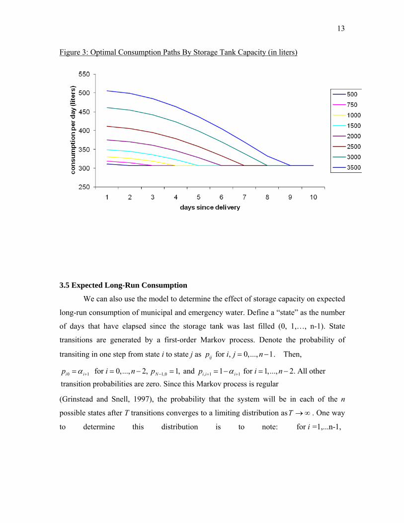
Figure 4 describes long-run expected daily consumption levels for agents with

storage tanks of different sizes. As the figure reflects, increasing the capacity of storage

increases average consumption, assuming the agent is capacity constrained. For a

sufficiently (i.e. unrealistically) large storage tank, it is possible for the agent to no longer

be capacity constrained.12 Figure 4 shows how expected daily consumption increases

with increases in capacity. This same methodology with the Markov process can be used

to calculate expected consumption for changes in other exogenous parameters such as

changes in water prices.13

12 As the storage tank increases, consumption on the period of resupply increases. The value of having additional water to consume in that period or later is . Provided that strictly exceeds the municipal price of water, it is optimal to fill the storage tank to capacity. Only if the storage tank is so large that

is it suboptimal to fill the tank to capacity.

0'( )U c

0'( )U c p<13 This steady-state distribution can no longer be used if it is assumed that uncertainty is eliminated since the Markov process is then no longer regular. However, when a group receives its water at regular intervals,,the stream of consumptions is deterministic and we can calculate the consumption path and resulting welfare directly.

15

Figure 4: Expected Consumption Levels by Storage Tank Capacity

4. A Calibration Exercise Using Microdata from Mexico City

4.1 Household Level Microdata

We calibrate the model for Mexico City using household-level microdata from the

Mexican National Household Survey of Income and Expenditure “Encuesta Nacional de

Ingresos y Gastos de los Hogares” (NHSIE) for 2005. The objective of the calibration is

to capture the welfare characteristics of the current system and to quantify the social

gains from moving to a system without uncertainty.

The NHSIE is a nationally representative household survey administered by

Mexico’s National Statistics Institute. The survey, which has been conducted

approximately every two years since 1984, serves as the basis for calculating the Mexican

Consumer Price Index and is widely used to construct measures of poverty and

inequality. The survey is administered in person and the national participation rate in

2005 was 88%. For our purposes, the NHSIE is valuable because it provides detailed

information about household water usage, as well as household demographics and

housing characteristics. With regard to water usage the survey asks households if they

have running water, how often they receive water deliveries, if they have water storage,

and typical monthly expenditure on water.

16

Households in Mexico City face great uncertainty about their water service. Water

provision has long been a daunting problem in Mexico City and our analysis is

particularly relevant to current policy aimed at extending water service to households on

the edge of the city. Although most residents of Mexico City receive municipal water

through pipes, often water is only available during particular hours of the day or days of

the week. In these cases water is turned on and off manually by special city water

regulators called valve workers or ``valvulistas’’. Because of the cities permanent water

shortage, as well as because of mechanical failures and human error, water service is

notoriously unreliable.14

In response to this uncertainty most households in Mexico City use some form of

private water storage. The most common form of water storage is a rooftop tank known

as a tinaco. In the NHSIE 44.78% of respondents reported having a tinaco. When this

tank runs dry, households typically respond by purchasing water from a tanker truck.

Trucks carry thousands of liters of water and can be hired to fill or partially fill household

tanks. Tanker trucks are widely used in Mexico City because of the chronic uncertainty

about water supply. Most of these trucks are privately-owned.15 The market for water

delivery is highly-competitive with near marginal-cost pricing. In the empirical

simulation, water delivered by tanker truck will serve as the backstop technology, the

“emergency” source of water when stored water has been completely depleted.

In Mexico City, municipal water and water from tanker trucks is used for bathing,

cleaning, and sanitation, but not for drinking or cooking. Even in households with very

limited resources, there is always a container of drinking water, typically 19 liters, known

as a garaffón. These containers of drinking water are delivered door-to-door by either

14 Water supply problems receive constant attention in the local media. Dozens of recent articles in a major Mexico City newspaper, El Universal, describe chronic water shortages in neighborhoods in most neighborhoods in Mexico City. See, e.g., “Fifteen Days Without Water Due to Pump Failure (Llevan 15 Días Sin Agua Por Avería en Bomba)” July 8, 2005; “Water Shortage in Coyoacán is Denounced (Denuncian Escasez de Agua en Coyoacán)” February 28, 2007; “Fourteen Delegations Suffer Water Shortage (Padecen Escasez de Agua en 14 Delegaciones)” July 1, 2007; “Increased Requests for Water Trucks in the Del Valle Neighborhood (En la Del Valle, Mayor Petición de Pipas de Agua en Juárez” July 23, 2007; “Residents of the Ajusco Neighborhood Refuse to Pay for Water They Don’t Receive (Se Niegan Vecinos de Ajusco a Pagar Agua Que No Reciben” December 16, 2007. 15 In some remote neighborhoods at the edge of Mexico City running water is unavailable and municipal water is delivered by truck rather than by pipes. In these neighborhoods both municipal and private trucks provide water. In the sample of households from Mexico City in the NHSIE, 1.8% of households reports receiving water by truck. These households are ignored in the empirical simulation.

17

truck or cart, and the supply-side of this market is private and highly-competitive with

few barriers to entry. In neighborhoods in Mexico City one often hears a gentleman

yelling, “Agua, Aguaaaa!” as he drives through the street delivering these containers.

Drinking water is virtually never used for non-drinking uses because it is much more

expensive than either municipal water, which is piped in, or water from tanker trucks. In

the empirical simulation that follows, we focus exclusively on non-potable water.

Because drinking water is provided by a large number of highly-competitive private

providers, there is virtually no uncertainty about drinking water availability in Mexico

City.

Since households do not drink or cook with municipal water, waterborne

pathogens are much less of a concern. This is reflected in the news accounts we have

examined. Municipal water provision in Mexico City features prominently in the local

news, but in the several years of articles we examined the focus is overwhelmingly on

water availability rather than on water quality. See, e.g., “Residents of the Ajusco

Neighborhood Refuse to Pay for Water They Don’t Receive (Se Niegan Vecinos de

Ajusco a Pagar Agua Que No Reciben)” El Universal, December 16, 2007 and the

articles cited in footnote 14. Accordingly, throughout the analysis we treat water quality

as constant.

Similarly, we assume that storage does not affect water quality. In many

developing countries private water storage has been shown to be a major concern with

respect to water quality (Kremer, Leino, Miguel and Zwane, 2006). This assumption is

likely to be a reasonable approximation in the current application because the tinacos

used to store water in Mexico City are sealed tanks, typically located on the roof and thus

protected from most sources of contamination. Ninety-percent of the market for tinacos

in Mexico is controlled by Rotoplas, a company that manufactures tinacos using heavy-

duty black plastic. Tank walls are constructed using a high-tech, multi-layered, anti-

bacterial surface that impedes the ability of microorganisms to reproduce inside the tank.

In addition, the black color is important because it prevents light from entering the tank,

18

reducing microbial and algae growth.16 The fact that the tinacos are sealed also implies

that evaporation is minimal. For use in other contexts, evaporation could be easily

accommodated in our model.

Thus, the private market has made considerable inroads in the water market in

Mexico City. The market for drinking water has been completely taken over by private

water providers. In the market for non-drinking water, the private delivery of non-

drinking water via tanker trucks provides a critical backstop technology, limiting the

social costs of uncertainty in municipal water provision. The reason the private market

has not evolved to play an even more important role in the market for non-drinking water

is that tanker trucks cannot offer water at the municipal water price because of operating

costs such as gasoline. Section 4.4 discusses water prices. Municipal water in Mexico

City is supplied at 2.86 Pesos per 1000 liters, equal to the marginal social cost of

supplying additional water through pipes. Even though the market for private water

delivery from tanker trucks is highly-competitive, prices for water delivered by private

tanker truck are still approximately 30 times as expensive as municipal water prices.

More generally, although there would be a market for privately-provided piped-in water,

the fixed costs of constructing and maintaining a water distribution network are large

enough to have prevented private entry.

4.2. Calibrating the Parameters of the Utility Function

In this subsection we solve the household’s utility-maximization problem to

derive the demand function for water and its price elasticity. We then calibrate the

parameters of the utility function using the observed level of demand in the NHSIE and

available estimates in the literature for price responsiveness.

In the standard case in which a household chooses each period the optimal

amounts of water and a composite commodity to consume given that it has income I and

faces water price p (both expressed in units of the composite commodity), the optimal

solution solves:

16 See “Rotoplas Paints Rooftops Black (Rotoplas, Pintan de Negro las Azoteas)” El Universal, March 15, 2006 for more information about Rotoplas and the dominance of black plastic tanks in the water storage tank market.

19

( ) (max .c

k c s I pcθ− + − )

The solution to the household’s problem may be expressed:

(3) 1

1* pc s

kθ

θ−⎛ ⎞= + ⎜ ⎟

⎝ ⎠ with the remaining income spent on the composite commodity.

Furthermore, taking the derivative of the demand function with respect to price and

multiplying by *c

p yields the price elasticity of demand for water,

(4) .*

11

**

11

ckp

cp

pc

−⎟⎠⎞

⎜⎝⎛

−==∂∂

θ

θθη

For the threshold for minimum consumption, we use 40 liters of water/person/day

following Gleick (1996).17 The households in the NHSIE sample in Mexico City have an

average of 3.82 members per household implying s=152.8 (40 * 3.82).

The curvature parameter θ and the scaling parameter k are calibrated using

available information about residential water demand. In particular, according the NHSIE

data, among household in Mexico City who have water available all days per week, all

hours per day, the average level of monthly expenditure on municipal water is 88.4

Pesos.18 The municipal water price of 2.86 Pesos per thousand liters, which will be

discussed in section 4.4, implies that these households consume on average 1013 liters of

water per day.19 This provides a benchmark level for c*. Also, a meta-analysis of recent

studies of residential water price elasticities, Dalhuisien, Florax, de Groot, and Nijamp

(2003) find an average price elasticity of η=-.41.

17 Gleick (1996) cites the U.S. Agency for International Development, the World Bank, and the World Health Organization, each of which recommend 20-40 liters of water/person/day. Accordingly, later in the paper we will also report results based on 20 and 30 liters of water/person/day. Gleick describes minimum daily usage by end use. Our baseline value of 40 liters of water/person/day is consistent with his recommended basic requirement for bathing, cleaning, and sanitation. 18 Households are asked about water expenditure twice in the NHSIE. Municipal water expenditure is included with expenditure on natural gas, electricity, and other utilities. Water expenditure is also elicited in a section about food and beverages. This presumably includes expenditure on drinking water. 19 This is consistent with Haggarty, Brook, and Zuluaga (2002) who report that water consumption in Latin American cities ranges from 200-300 liters per day per person.

20

Using these two benchmarks, together with the demand function for water and the

expression for the price elasticity, we solve for θ and k. In particular, substituting (3) into

(4) and rearranging yields

*1 1*

c sc

θη−

= + = − .07 .

From (3), .3194)*( 1 −=

−= −θθ sc

pk

The resulting utility function is increasing and concave in water consumption (see

footnote 9) and can be used to compare the value of different levels of water consumption

in units of the composite good. Finally, we use a daily discount rate β=.999813. This

corresponds to where r is the Interbank Equilibrium Interest Rate (TIIE) calculated by

The Mexican Central Bank (Banco de México) as of 6/12/2007, a 7.705% annualized

interest rate if compounded daily.20 In section 4.7 we consider alternative assumptions

about the rate of time preference.

4.3 Water Storage in Mexico City

There are several different sizes of tinacos used in Mexico City. Because of

weight and size considerations, however, few households have tinacos larger than 1000

liters. According to our conversations with hydraulic engineers in Mexico City, the most

common size of tinaco in Mexico City is 750 liters. In our benchmark specification we

assume that each household has 750 liters of water storage. In section 4.7 we evaluate the

robustness of our results to alternative assumptions about tinaco size. As a point of

comparison, notice that a 750-liter tinaco holds approximately 75% of what the average

Mexican household would consume in a single day if it had continual access to municipal

water. Hence, as long as water must be stored, consumption of water is inevitably

restricted.

20 For calibration purposes we are setting , which will be true in equilibrium as long as households are consuming some of the composite commodity in each period. In this case the marginal rate of substitution between consumption in period t and consumption in period t+1 is simply and the price required to induce this consumption is 1+r.

21

This naturally raises the question of why households in Mexico City do not equip

themselves with larger tinacos. For example, our earlier simulations suggest that a 5000

liter tinaco would allow the household to almost perfectly smooth consumption.

However, tinacos must be located on roofs to take advantage of gravity. The weight and

volume of water which roofs can accommodate constitute limiting factors. Even 1000

liters of water weighs 1000 kilograms or 2200 pounds, a weight requiring substantial

structural reinforcement. Although our model does indicate that there are potentially large

private gains from increased water storage, these practical limitations typically limit

storage to approximately 750 liters.

4.4 Water Service Uncertainty in Mexico City

Table 1 describes the frequency of water deliveries across households in Mexico

City. The NHSIE data reveal that 32.0% of households in Mexico City are subject to

some form of water uncertainty and 10.4% receive water less frequently than once per

day. This is consistent with Haggarty, Brook, and Zuluaga (2002) who report that over

half of all neighborhoods in Mexico City routinely suffer cuts in service, with some

residents, particular in the southern and southeastern portions of the city receiving water

less than once per week.21

The table also reports the percentage of households from each category who

report having water tanks. Several comments are worth making. First, most households

have water tanks, including homes which report having daily water deliveries.

Households with water all hours all days are likely using their tinacos for water pressure

purposes rather than for storage. Second, there is an overall pattern in which households

with less frequent deliveries are more likely to have tinacos. This is particularly

pronounced for households with extremely infrequent water deliveries.

21 We also examined delivery frequencies for the rest of Mexico and results are similar. Uncertainty is particularly prevalent in the Mexico’s central region where water is most scarce. Over thirty percent of households receive water less than once per day in the Mexican states Puebla (33%), Hidalgo (37%), Queretaro (44%), Nayarit (47%) and Morelos (47%).

22

Table 1: Households in Mexico City in the NHSIE

Frequency Percentage with

Tinaco

One day per week 2.8% 95.2%

Two days per week 2.1% 86.7%

Three days per week 3.8% 68.8%

Four days per week 0.2% 80.0%

Five days per week 1.3% 100.0%

Six days per week 0.2% 50.0%

Daily at limited hours 21.6% 74.9%

Daily at all hours 68.0% 67.2%

Note: Frequency of water deliveries comes from the

NHSIE. The total sample includes 843 households.

From these data we construct an alpha path describing water supply uncertainty

for each household type. For households who receive water on average once per week,

we adopt an alpha path of [1/7, 1/7, 1/7, ……]. Thus for these households, the

probability that water is resupplied on day i is geometrically distributed with parameter

1/7. 22 We treat households that report receiving an average of two deliveries per week as

if they draw delivery times from a geometric distribution with parameter 2/7.

In order to calibrate the model we also need water prices. Figure 5 describes

residential water prices for 21 large cities in Mexico.23 The mean water price across cities

is 3.94 Pesos ($0.35 in U.S. 2005 dollars) per 1000 liters. For the calibration we use the

22 To be consistent with the model we impose the condition that αn=1, for a value of n sufficiently large that the household is virtually certain to be resupplied before then Even for a household that receives water deliveries once per week, the probability of not being resupplied for n consecutive periods is less than 1 in 10 million. Although this results in a geometric distribution that is truncated on the right, its mean is only trivially less than that of its untruncated counterpart. 23 National Water Commission (Comision Nacional de Agua), 2004.

23

price of municipal water in Mexico City of 2.86 Pesos ($0.25) per 1000 liters.24 As a

point of comparison, according to Raftelis (2005), the mean residential water price in the

United States is $1.17 per 1000 liters.

Figure 5: Water Prices in Selected Mexican Cities

0

0.002

0.004

0.006

0.008

0.01

0.012

Tijua

na

La P

az

Manza

nillo*

Nuevo

Lared

o

Chihua

hua

Cancu

n

Chetum

al

Guada

lajar

a

Hermos

illo

Zaca

tecas

Culiac

an

Juare

z

Xalapa

Colima*

Distrito

Fed

eral*

Mexica

li

San Lu

is Poto

sí

Tampic

o Mad

ero

Mérida

*

Morelia

Campe

che

City

Pes

os/L

Another important model parameter is the price of emergency water. As discussed

in section 4.1, in Mexico City when municipal water does not arrive and households run

out of water in their tinacos, they typically respond by purchasing water from a private

water delivery truck. There is no comprehensive source of information for these prices,

and in a review of newspaper articles we found prices ranging from 50-200 Pesos per

1000 liters.25 Thus for the baseline emergency price of water we use p̂ =100 Pesos

($8.88 in U.S. 2005 dollars) per 1000 liters. Later in the paper we also report results for

p̂ =50 and p̂ =200. 24 We have confirmed this water price using actual residential water bills from Mexico City. It is also worth emphasizing that whereas there are relatively large differences in water prices across Mexican cities, water prices within Mexico City are highly uniform. 25 For prices of water delivered by tanker trucks see "Those Affected by Leak Denounce Water Abuses (Afectados por Fuga Denuncian Abusos con Agua)", El Universal, June 8, 2008 and "Residents Protest Lack of Water: Eight Neighborhoods in Chimalhuacán Affected (Colonos Protestan por Falta de Agua: Ocho barrios de Chimalhuacán, Los Afectados)" El Universal, October 31, 2006. We also corresponded with Firdaus Jhabvala, water expert and director of the Center for Southeastern Research (Centro de Estudios de Investigación del Sureste) and were provided in personal correspondence a price that is very similar to our baseline price of 100 Pesos per 1000 liters.

24

The emergency price of water is assumed to be exogenous. If the marginal cost of

wate for tankr er trucks is not constant, one might have instead expected the emergency

price of

timal Consumption under Uncertainty

Our model enables us to determine the optimal contingent consumption vector for

cludes consumption of municipal water

tegy for households that on

averag

water to be correlated with the level of demand. For example, if the marginal cost

curve is upward sloping, the price would fall when demand decreases. This is potentially

important in our analysis because we want to be able to describe how welfare would

change under alternative forms of water provision including programs that decrease water

uncertainty and thus decrease demand for emergency water. Although data are not

available to evaluate this possibility empirically, for a number of reasons we believe

constant marginal cost is a reasonable approximation. Tanker trucks typically fill their

tanks wherever water is available including municipal sources. Water is always available

somewhere at the municipal price, and tanker trucks can fill their tanks and then travel to

neighborhoods where water is not available. Furthermore, tanker trucks supply other

users of water. For example, industrial customers and producers of drinking water

demand water from these same sources and when emergency water demand shifts inward

in our counterfactuals, demand for these other uses of water from tanker trucks does not

shift.

4.5 Op

each type of consumer. The optimal strategy in

and emergency water. Households rely on municipal water until they have exhausted

their tinacos, and then consume water from emergency sources. At one extreme are

households with such frequent water deliveries that they do not use emergency water at

all. For example, households that receive water daily during limited hours are predicted

to consume only municipal water because the emergency price of water exceeds the

marginal utility of water consumption for these households.

At the other extreme are households that receive water infrequently. For example,

Table 2 describes the optimal contingent consumption stra

e receive water once per week.

25

Number of days since last delivery Daily Consumption (liters)

0 331.391 319.012 307.423 307.424 307.425 307.426 307.427 307.428 307.429 307.42

10 307.42100 307.42

Table 2: Optimal Consumption Strategy

During the day of resupply and the following two days, such households consume

at a decreasing rate their stored municipal water. Unless re-supplied, these households

drain their tinaco during the third day after the last delivery, and supplement this stored

municipal water with emergency water.26 After this one period of transition, they rely

exclusively on emergency water until the arrival of the cheaper municipal water.

If they followed this contingent strategy repeatedly, in the long run the probability

of their being in each contingent consumption state converges to a stationary distribution

(see section 3.5) with expected total consumption of 312.3 liters, 78.26 liters of which

comes from the municipality.

Table 3 describes expected long-run water consumption for households which

receive water at different mean intervals. 68% of households have access to water at all

hours and consume such that '( ) ,U c p= implying daily household consumption of 1013

liters per day. The remaining 32% of the households have less frequent water service and

consume more emergency water but less water overall. For example, households with an

average of one delivery per week consume only about thirty percent (312.3/1013.0), of

the water consumed by households that receive water daily at all hours. Most of the water

consumed by these households is from emergency water sources rather than municipal

water. Since only 96.9 liters of the 312.3 liters consumed daily (31%) comes from the

municipality, the average price per liter paid for water by these households is very high, 26 Having consumed approximately 600 liters at that point, they would deplete the remaining 150 liters of their tinaco and supplement it with 43 liters of emergency water to provide the 193 liters of predicted consumption.

26

70 Pesos (per 1000 liters). Overall, the average price paid for water, 7, far exceeds the

municipal price of 2.86. Table 3 demonstrates that water uncertainty severely lowers

water consumption, particularly for households that receive water only a few times per

week.

Table 3: Water Consumption in Mexico City

Average Number of Deliveries per Week

% of Households

(NHSIE)

Average Daily Total

Consumption in Liters (Simulation)

Average Daily Consumption from the Municipality in Liters (Excluding

Emergency Water, Simulation)

Average Price Per

1000 Liters Paid for Water

(Pesos)

1 2.84% 312.3 96.9 70

2 2.08% 328.9 179.7 47

3 3.78% 358.1 257.7 30

4 0.19% 376.4 319.9 17

5 1.33% 400.9 375.8 9

6 0.19% 489.1 473.4 6

Daily at limited hours 21.55% 750.0 750.0 3Daily at all hours (water available continuously) 68.04% 1013.0 1013.0 3

Weighted Averages- 887.1 873.6 7

The severe reduction of water consumption observed in Table 3 provides a

possible explanation as to why the government tolerates the haphazard delivery of water.

Infrequent and uncertain deliveries of water reduce average water consumption,

providing a mechanism for allocating scarce water without raising the price or inducing

queues. One might call the regime “rationing by shadow price.” If water were always

available, the price p would generate excess demand. Uncertainty can be seen either as an

inevitable product of this shortage, or as a strategy used by the water administrator to

allocate water in the presence of the shortage.27 The costs of the system, the large

inefficiencies which are so inequitably distributed, are largely hidden.

27 An interesting dynamic issue may arise when uncertainty is used as an explicit strategy for addressing excess demand. Suppose, for example, that an exogenous increase in population increases demand for

27

4.6 The Welfare Comparison

The model can be used to examine the welfare implications of alternative modes

of water provision. We first consider providing water at regular, equally-spaced intervals

to the 32% of the households who currently receive water haphazardly; the remaining

households would continue to receive water at all hours. Second, we consider providing

water continuously to all households. Unlike the first counterfactual, the second requires

a modest increase in the price of municipal water in order to keep total water

consumption equal to water consumption under the status quo; we assume that an equal

share of the increase in these revenues is rebated to each household as a lump-sum

transfer.

In the first counterfactual, we normalize the time between deliveries for all

households not currently receiving continuous water provision. Instead of some

households receiving water once a week and others receiving seven times per week, we

assume that all households receive water at the same time interval. This reduces the large

differences between households. In addition, by providing the water at fixed intervals,

households are able to perfectly smooth water consumption, eliminating the inefficiency

caused by uncertainty.

The first counterfactual is implemented as follows. Notice that in the status quo,

68% of households receive water continuously. It would be politically difficult and

extremely expensive to move these households to a system without continuous water

provision because this would require these households to purchase and install tinacos.

Instead, for the first counterfactual we continue to provide water continuously to these

households, but normalize the delivery interval for the remaining 32% of households.

The model implies a total level of water consumption for any given such interval. We

select the delivery interval (every 31.2 hours) such that total water consumption under the

first counterfactual is equal to total water consumption under the status quo. Notice that

water above the available supply at the fixed municipal price. In order to address this excess demand, the water administrator increases the level of uncertainty of provision. However, this may cause households to respond by increasing storage capacity. This further increases demand, leading the water administrators to implement an additional increase in the level of uncertainty.

28

the first counterfactual requires: (1) no water price increase and (2) no additional

infrastructure.28

The second counterfactual we consider is providing water to all households daily

at all hours of the day. This counterfactual completely eliminates the need for the private

storage of water, freeing households from future purchases of tinacos and related

maintenance expenses. Furthermore, such a system is efficient, because it equates the

marginal utility of consumption across all households and time periods. Under the second

counterfactual all households consume the same amount of water and have the same level

of utility.

Moving to a system of continuous water provision at current water prices will

cause water consumption to increase. In this application, at current water prices all

households would consume 1013 liters per day. However, it may be the case that existing

water supply sources and/or the municipal distribution infrastructure is not sufficient to

meet this increase in demand. Indeed, as mentioned before, this lack of supply is one of

the primary public rationales for the current system.

Instead, it is more reasonable to ask how high the price would need to be in order

to maintain average water consumption at the same level while making water available at

all hours. Under the current system, the average household consumes 887 liters per day,

873.6 liters per day from the municipal system. In order to implement a system where

water is provided at all hours but maintains this level of demand, it is necessary to raise

the price of municipal water to p* such that '( *) *U c p= where c* = 873.6. In our

application p*=4.12 Pesos ($0.37 dollars).29 At this price total consumption of municipal

28 Average daily consumption of municipal water is 873.6 liters per day, but that average is elevated by the inclusion of that segment of the populace which has water available continuously. The remaining 31.96% of the residents must cutback their usage over time to make do until the next delivery arrives and then sharply raise their usage, on average consuming municipal water at a rate of 577.3 liters every 24 hours. Hence, if these residents were all certain that their 750 liter tinaco would be resupplied every 31.2 hours, they could consume indefinitely at the steady rate of 577.3 liters per day, thereby smoothing their consumption perfectly. 29 The price increase causes municipal revenue to increase. In order to facilitate the comparison with the status quo, we return this increased revenue to households in a lump-sum transfer equal to the average increase in expenditure per day, equal to mean consumption per day*(new price per unit--initial price per unit) = 873.6*(.00412-.00286)=1.1 Pesos per day or, present discounted value of 5907 Pesos. This assumption only negligibly affects the reported measures of welfare gain, and changes none of the qualitative results.

29

water is the same as it is under the status quo. This represents a 44% increase over the

original municipal price.30

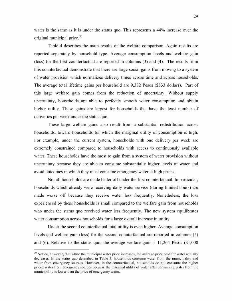
Table 4 describes the main results of the welfare comparison. Again results are

reported separately by household type. Average consumption levels and welfare gain

(loss) for the first counterfactual are reported in columns (3) and (4). The results from

this counterfactual demonstrate that there are large social gains from moving to a system

of water provision which normalizes delivery times across time and across households.

The average total lifetime gains per household are 9,382 Pesos ($833 dollars). Part of

this large welfare gain comes from the reduction of uncertainty. Without supply

uncertainty, households are able to perfectly smooth water consumption and obtain

higher utility. These gains are largest for households that have the least number of

deliveries per week under the status quo.

These large welfare gains also result from a substantial redistribution across

households, toward households for which the marginal utility of consumption is high.

For example, under the current system, households with one delivery per week are

extremely constrained compared to households with access to continuously available

water. These households have the most to gain from a system of water provision without

uncertainty because they are able to consume substantially higher levels of water and

avoid outcomes in which they must consume emergency water at high prices.

Not all households are made better off under the first counterfactual. In particular,

households which already were receiving daily water service (during limited hours) are

made worse off because they receive water less frequently. Nonetheless, the loss

experienced by these households is small compared to the welfare gain from households

who under the status quo received water less frequently. The new system equilibrates

water consumption across households for a large overall increase in utility.

Under the second counterfactual total utility is even higher. Average consumption

levels and welfare gain (loss) for the second counterfactual are reported in columns (5)

and (6). Relative to the status quo, the average welfare gain is 11,264 Pesos ($1,000 30 Notice, however, that while the municipal water price increases, the average price paid for water actually decreases. In the status quo described in Table 3, households consume water from the municipality and water from emergency sources. However, in the counterfactual, households do not consume the higher priced water from emergency sources because the marginal utility of water after consuming water from the municipality is lower than the price of emergency water.

30

dollars). Whereas the first counterfactual reduced differential allocation of water across

households, the second counterfactual treats all households identically. Again, there is

one group of households that is made worse off. In particular, households who under the

status quo had continuous access to water are made worse off because of the price

increase. Notice, however, that the loss in welfare for these households is small relative

to the gain for other households. Because the second counterfactual is efficient, it would

be possible with an appropriate system of lump-sum transfers, to make all households

strictly better off.31

Although our first counterfactual garners nearly as much welfare gain as the

second counterfactual and is much cheaper to implement, one caveat should be kept in

mind. Our assumption that consumers have identical marginal utility schedules and

identical sized tinacos contributes to our finding since, under this assumed homogeneity,

the policy of uniform deliveries completely eliminates the distributional inefficiency

among 32% of the households. To the extent that this group is heterogeneous, an

inefficiency would remain under this policy and the resulting welfare gain might be

smaller.

31 In our simulations, we assume that providers of emergency water receive no lump-sum transfers. Although these providers would be put out of business once the cheaper municipal water became available on a daily basis, they would not be worse off unless they had been earning rents due either to market power or to scarce capacity. If they were earning such rents, there would be revenues sufficient to compensate these providers as well as the consumers. This follows since the second counterfactual is distributionally efficient.

31

Table 4: The Welfare Implications of Alternative Modes of Water Provision

Status Quo Counterfactual #1 Households type 1-7 provided

water at same interval

(every 31.2 hours)

Counterfactual #2 Water Provided Daily at all

hours to all households, with a

price increase to clear market

Average Number of

Deliveries Per Week

Average Daily Water

Consumption from the

Municipality (in liters)

Average

Daily Water

Consumption

(in liters)

Welfare Gain

(Loss)

Relative to

Status Quo

Average

Daily Water

Consumption

(in liters)

Welfare Gain

(Loss)

Relative to

Status Quo

(in Pesos) (in Pesos)

1 96.9 577.3 156,539 873.6 163,331

2 179.7 577.3 116,012 873.6 122,804

3 257.7 577.3 82,376 873.6 89,169

4 319.9 577.3 55,152 873.6 61,945

5 375.8 577.3 34,375 873.6 41,167

6 473.4 577.3 17,899 873.6 24,691

Daily at limited hours 750.0 577.3 (5,370) 873.6 1,421

Daily at all hours (water

available continuously) 1013.0 1013.0 0 873.6 (430)

Weighted Averages 873.6 873.6 9,382 873.6 11,264

32

Table 5: Sensitivity Analysis

Welfare Gain Relative to Status Quo (in Pesos)

Water Provided Daily at all hours to all

households, with a price increase to clear market

Baseline Estimate 11,264 Rate of Time Preference (7.705% annualized rate) 5.0% annualized rate 15,760 10% annualized rate 8,066 Minimum Consumption Level (40 liters/person/day) 30 liters/person/day (s=114.6) 9,763 20 liters/person/day (s=76.4) 8,317 Curvature Parameter (θ=-1.071) θ=-.90 19,838 θ=-1.2 8,486 Tinaco Size (750 liters) liters 500 liters 15,475

liters 1000 liters 9,449 1500 liters 7,756 750/1000 liters 9,793

Emergency Price (100 Pesos per 1000 liters) 50 Pesos per 1000 liters 7,235 200 Pesos per 1000 liters 17,449 Note: This table reports the main results for 13 different sets of model parameters. For each specification, the table reports the average annual gain in household welfare that corresponds to a transition to a system of water provision in which water uncertainty is removed and the price of water is increased in order to clear the market (the last column in table 4). Baseline parameters are indicated in parentheses. Amounts are in 2005 Pesos. For 2005 dollars divide by 11.26.

33

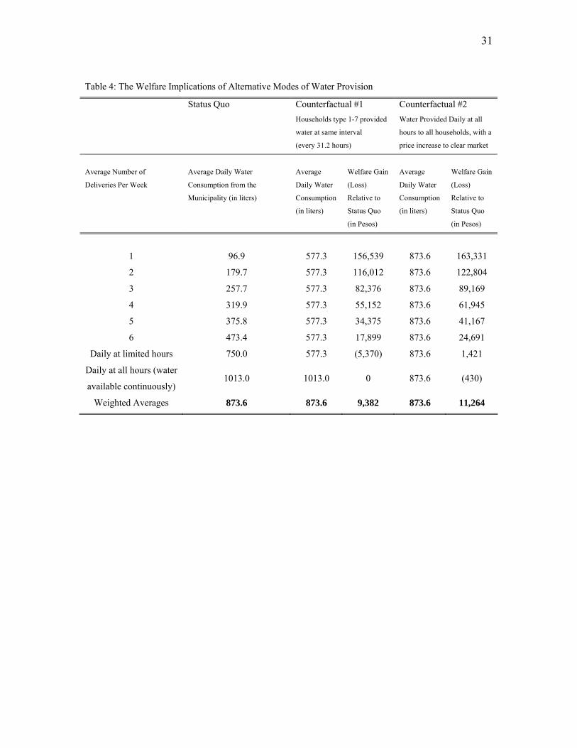
4.7 Sensitivity Analysis

Sections 4.5 and 4.6 provide results for our baseline parameters. In this subsection

we examine the sensitivity of the results to alternative parameter choices. For each

specification, the table reports the average annual gain in household welfare that

corresponds to a transition to a system of water provision in which water uncertainty is

removed and the price of water is increased in order to clear the market (the last column

in table 4). Overall, the results are relatively insensitive to minor changes in the

parameters.

First, table 5 reports the simulated change in welfare under alternative

assumptions about the rate of time preference. The baseline results use a daily discount

rate of where r is the Interbank Equilibrium Interest Rate (TIEE), a 7.705%

annualized interest rate if compounded daily. The TIEE is the most commonly used

interest rate in Mexico. Although the TIEE is a valuable starting point, it is valuable to

examine how the results change with alternative assumptions about β. Although home

and car loans are widely-available in Mexico City, credit cards and other forms of

household credit are less common than they are in the United States. In particular, many

households in Mexico City do not have easy access to credit at the relatively-low TIEE

rate. For a 10% rate the change in welfare is 8,066 Pesos (28.4% lower). For

completeness, we also considered an alternative specification with a lower interest rate.

For a 5% annualized rate the change in expected discounted welfare is 15,760 Pesos

(39.9% higher).

Second, table 5 reports the change in welfare under alternative values for s, the

minimum consumption level. Recall that in the empirical simulation utility from water

consumption in each period is k(c-s)θ where s is the threshold for minimum daily

consumption. For the baseline value for s we use 152.8 which corresponds to 40 liters of

water/person/day. For 30 and 20 liters of water/person/day the change in welfare is 9,763

Pesos (13.3% lower) and 8,317 Pesos (26.2% lower). With smaller minimum

consumption levels the change in welfare is smaller because the household consumes less

water with and without uncertainty.

Third, we considered alternative values for θ, the curvature parameter. Recall that

in our utility function both k and θ are negative so utility is increasing and concave in

34

water consumption. In our baseline specification we used θ=-1.071 and for alternative

specifications we adopted -0.9 and -1.2. With -0.9 the change in expected discounted

welfare is 19,838 Pesos (76.1% higher) and with -1.2 the change in welfare is 8,486

(24.7% lower). Increasing the curvature parameter (away from zero) causes the marginal

utility of water consumption to decrease more quickly, increasing the motive for

consumption smoothing and decreasing the level of water consumption under both

certainty and uncertainty.

Fourth, we consider what happens to the change in welfare when we change

tinaco size. In the baseline specification we assume that all households have 750 liters of

water storage. Although the NHSIE asks households whether they have a tinaco or not, it

does not ask households about tank size. As discussed in section 4.3, there are practical

considerations, most importantly weight, that provide limits on tank size in most

dwellings. Still, the model implies that households, particularly in neighborhoods facing

severe uncertainty, have large incentives to increase their storage capacity and indeed

some households in Mexico City have gone to greater lengths to store water privately, for

example, by constructing underground tanks that are connected to the rooftop tinacos.

Table 5 reports the welfare change relative to the status quo for alternative

assumptions about tinaco size. We consider the cases with 500, 1000 and 1500 liter

tinacos. Although 1500 liter tinacos are very unusual in Mexico City, this counterfactual

is useful for understanding how the model works and for simulating a case in which

households have some form of additional water storage capacity in addition to tinacos.

As expected, the welfare gains from eliminating uncertainty are decreasing in tank size.

With 1500 liter tinacos the welfare gain from eliminating uncertainty is 7,756 Pesos

(31.1% smaller).

This counterfactual still ignores, however, the likelihood that in reality customers

with different needs for storage may have purchased tinacos of different sizes. Most

tinacos used in Mexico City are produced by a company called Rotoplas. Though

evidence from our interviews indicates that 750 liter tinacos are the most popular,

Rotoplas produces several different sizes of tinacos including 500, 750, 1000, and 1100-

liter models. We would expect this choice of which tinaco to buy to be correlated with the

35

irregularity of service. Not allowing for this heterogeneity in the simulation likely biases

upward our estimates of the welfare costs of uncertainty because the households with the

most to gain from increased capacity would be among the first to invest in larger tanks.

Table 5 provides evidence about the potential magnitude of this bias. In this

counterfactual, we assume that there are two different tinaco sizes, 750 and 1000 liters.

Furthermore, we assign systematically the larger tinacos to households with the greatest

need for storage capacity. In particular, households who receive water 1-4 days per week

are assigned 1000-liter tinacos and households who receive water 5-6 times per week or

daily at limited hours are assigned 750-liter tinacos. Under this counterfactual the present

value of the expected welfare gain relative to the status quo is 9,793 Pesos (13.1% lower).

However, since the average capacity across households in this specification is 22.2 liters

larger than in the benchmark, a small part of this 13.1% results from the increase in the

average tinaco size.32 As expected, increasing tinaco size for these households decreases

the gain relative to the status quo because these households are better able to smooth

consumption under uncertainty.

Finally, we consider the effect of changing the price of emergency water. For the

baseline emergency price we use 100 Pesos per 1000 liters of water. As discussed above,

however, in practice the price of water from tanker trucks ranges from 50-200 Pesos per

1000 liters. As demonstrated in table 5, the emergency price has the expected effect on

household welfare. For emergency prices of 50 Pesos per 1000 liters, households use

municipal water more freely, are better able to smooth consumption and the welfare gain

relative to status quo is 7,235 Pesos (35.8% smaller). For an emergency price of 200

Pesos per 1000 liters, the expected discounted welfare gain is 17,449 Pesos (54.9%

larger).

32 Since the expected present value of the welfare gain if every household had a tinaco of 772.2 liters is 11,056 Pesos, the pure effect of introducing heterogeneity is to lower the welfare gain by 11% rather than 13%.

36

5. Concluding Remarks

This paper has examined the welfare costs of water delivery uncertainty.

Municipal water administrators are afraid to raise water prices (see Timmins 2002), and

supplying water infrequently offers one mechanism for eliminating the excess demand

caused while pricing below the market clearing level. These systems are particularly

popular in the developing world where the political pressure to keep water prices low is

strong. Unfortunately, there are large welfare costs from water supply uncertainty and

these costs are borne by those with infrequent deliveries and/or smallest storage

capacities.

The problem with supply uncertainty is that it prevents water from being allocated

to the buyers who value it the most. In this paper we described a model of water

consumption in which households solve a dynamic optimal consumption problem in the

face of uncertainty about the availability of water. Misallocation may frequently occur in

this context, with one household desperate for water while another is allocating water to

frivolous uses. And yet, without a market mechanism there is no way that the parched

family can acquire the water the other family is wasting. We described the properties of

the model, demonstrating how the introduction of uncertainty, changes in emergency

water prices, and changes in storage capacity affect water consumption and welfare.

We then calibrated the model using household-level microdata from a random

sample of households in Mexico City in order to measure the welfare costs of uncertainty

in a typical water system. We solved the model for a set of representative households and

quantified the social gains from moving either to a two-tier system where everyone now

storing water would receive deliveries at the same frequency or to a system where all

households have access to water at all hours. The results demonstrate that the gains in

distributional efficiency from reliable water service are very large in magnitude.

Moreover, most of those gains can be achieved simply by normalizing the delivery

schedules of those now storing water so that the frequency of deliveries is the same for

these households. This can be achieved without costly changes in infrastructure, price

increases, or rebates.

In future work it would be interesting to consider how our results would change if

we adopted a collective model of household behavior. The current model assumes that

37

the household acts as a single decision-maker (the so-called “unitary” model) rather than

as a collection of individual decision-makers, each pursuing his or her self-interest (the

“collective model”). See, e.g. Fortin, Bernard and Guy Lacroix (1997). Intra-household

interactions would likely exacerbate the inefficiencies from water supply uncertainty. In

each period, every household member would consume water out of the tank until his (or

her) marginal benefit of consuming one more unit of water currently is equal to his

discounted marginal cost of having one less unit of water in the tinaco next period.

However, since water in the tinaco is shared with other family members, each individual

would bear only a fraction of the full future cost of removing water from the tank. This

would lead to aggregate overuse of water in the tinaco relative to the unitary case---a

within-household tragedy of the commons; as a result, the household would bear even

larger costs during periods of limited water availability. The model of Levhari and

Mirman (1980), formulated to study the subgame perfect equilibrium of a two-player,

finite-horizon multistage game where simultaneous extraction depletes an otherwise

expanding fish stock, is easily specialized to our no growth case of pure depletion and

generalized to any finite number of extractors from a common pool. Whether this model

can also be adapted to our infinitely repeated stochastic environment remains for future

work. If their model could be adapted, one could repeat the exercises we perform here.

References

Alcázar, Lorena, Lixin Colin Xu and Ana M. Zuluaga. 2002. “Institutions, Politics, and Contracts: The

Privatization Attempt of the Water and Sanitation Utility of Lima, Peru,” in Thirsting for

Efficiency: The Economics and Politics of Urban Water System Reform, Mary M, Shirley (ed,),

World Bank.

Comision Nacional de Agua (CNA). Situacion del Subsector Agua Potable, Alcantarillado y Saneamiento.

Government Publication, December 2004.

Dalhuisien J., Florax R., H. de Groot, and Nijamp P. 2003. Price and Income Elasticities of Residential

Water Demand: A Meta-Analysis. Land Economics, May.

Famsa.com. Tinacos. Accessed April 11, 2007. http://www.famsa.com/webapp/wcs/stores

38

/servlet/CategoryDisplay?catalogId=10001&storeId=10001&categoryId=10215&langId=-

5&parent_category_rn=10106

Fernandez Emilio. 2006. Water most expensive for city’s poorest. Miami Herald, April 24.

Fortin, Bernard and Guy Lacroix. “A Test of the Unitary and Collective Models of Household Labour

Supply”, The Economic Journal, 1997, 107 (443), 933–955.

Gleick, Peter H. 1996. ``Basic Water Requirements for Human Activities: Meeting Basic Needs"

Water International, 21, 83-92.

Grinstead, Charles M. and J. Laurie Snell. 1997. Introduction to Probability: Second Revised Edition.

Dartmouth College.

Haggarty, Luke, Penelope Brook and Ana Maria Zuluaga. . 2002. “Water Sector Service Contracts in

Mexico City, Mexico,” in Thirsting for Efficiency: The Economics and Politics of Urban Water

System Reform, Mary M, Shirley (ed,), World Bank.

Hotelling, Harold. 1931. The Economics of Exhaustible Resources. Journal of Political

Economy, April.

Instituto Nacional de Estadística Geografia e Informática (INEGI). 2006. Encuesta Nacional de

Ingresos y Gastos de los Hogares (NHSIE).

http://www.inegi.gob.mx/est/contenidos/espanol/sistemas/enigh/bd/default.asp

Kremer, Michael, Jessica Leino, Edward Miguel, and Alix Peterson Zwane. 2006. Spring Cleaning: A

Randomized Evaluation of Source Water Quality Improvement. Unpublished manuscript.

Levhari, David and Leonard J. Mirman. 1980.The Great Fish War: An Example Using a Dynamic Cournot-

Nash Solution. The Bell Journal of Economics, 11(1), 322-334.

Long, Ngo Van. 1975. Resource extraction under the uncertainty about possible nationalization. Journal of

Economic Theory 10, 42-53.

Porter, Richard C., The Economics of Water and Waste in Three African Capitals (Accra, Harare,

Gaborone), Ashgate Press: 1997.

Raftelis Financial Consulting, PA, 2005. Water and Wastewater Rate Survey. Charlotte, North Carolina.

Salant, Stephen., Henderson, Dale. 1978. Market Anticipation of Government Policies and the Price of

Gold. Journal of Political Economy, August.

Soto Montes de Oca, G., and I. J. Bateman. 2006. Scope sensitivity in households’ willingness to pay for

maintained and improved water supplies in a developing world urban area: Investigating the

influence of baseline supply quality and income distribution upon stated preferences in Mexico

City. Water Resources. Research., Vol 42.

Timmins, Christopher. 2002. Measuring the Dynamic Efficiency Costs of Regulators’ Preferences:

Municipal Water Utilities in the Arid West. Econometrica, 70(2), 603-629.

Whittington, Dale. Lauria, Donald L. 1991. A Study of Water Vending and Willingness to Pay for Water in

Onitsha, Nigeria. World Development, Vol 19, No. 2/3.