The Welfare Cost of Asymmetric Information: Evidence … · markets and the potential for welfare-improving government intervention. ... of individuals receiving different insurance

The Welfare Cost of Asymmetric Information:Evidence from the U.K. Annuity Market∗

Liran Einav, Amy Finkelstein, and Paul Schrimpf†

May 29, 2007

Abstract. Much of the extensive empirical literature on insurance markets hasfocused on whether adverse selection can be detected. Once detected, however, there has

been little attempt to quantify its importance. We start by showing theoretically that

the efficiency cost of adverse selection cannot be inferred from reduced form evidence of

how “adversely selected” an insurance market appears to be. Instead, an explicit model

of insurance contract choice is required. We develop and estimate such a model in the

context of the U.K. annuity market. The model allows for private information about risk

type (mortality) as well as heterogeneity in preferences over different contract options.

We focus on the choice of length of guarantee among individuals who are required to

buy annuities. The results suggest that asymmetric information along the guarantee

margin reduces welfare relative to a first-best, symmetric information benchmark by

about £127 million per year, or about 2 percent of annual premiums. We also find

that government mandates, the canonical solution to adverse selection problems, do

not necessarily improve on the asymmetric information equilibrium. Depending on the

contract mandated, mandates could reduce welfare by as much as £107 million annually,

or increase it by as much as £127 million. Since determining which mandates would

be welfare improving is empirically difficult, our findings suggest that achieving welfare

gains through mandatory social insurance may be harder in practice than simple theory

may suggest.

JEL classification numbers: C13, C51, D14, D60, D82.

Keywords: Annuities, contract choice, adverse selection, structural estimation.

∗We are grateful to James Banks, Richard Blundell, Jeff Brown, Peter Diamond, Carl Emmerson, Jerry Hausman,

Jonathan Levin, Alessandro Lizzeri, Wojciech Kopczuk, Ben Olken, Casey Rothschild, and seminar participants at

the AEA 2007 annual meeting, Chicago, Hoover, Institute for Fiscal Studies, MIT, Stanford, Washington University,

and Wharton for helpful comments, and to several patient and helpful employees at the firm whose data we analyze.

Financial support from the National Institute of Aging (Finkelstein), the National Science Foundation (Einav), and

the Social Security Administration is greatfully acknowledged. Einav also acknowledges the hospitality of the Hoover

Institution.†Einav: Department of Economics, Stanford University, and NBER, [email protected]; Finkelstein: Department

of Economics, MIT, and NBER, [email protected]; Schrimpf: Department of Economics, MIT, [email protected].

1 Introduction

Ever since the seminal works of Akerlof (1970) and Rothschild and Stiglitz (1976), a rich theoret-

ical literature has emphasized the negative welfare consequences of adverse selection in insurance

markets and the potential for welfare-improving government intervention. More recently, a grow-

ing empirical literature has developed ways to detect whether asymmetric information exists in

particular insurance markets (Chiappori and Salanie, 2000; Finkelstein and McGarry, 2006). Once

adverse selection is detected, however, there has been no attempt to estimate the magnitude of its

efficiency costs, or to compare welfare in the asymmetric information equilibrium to what would

be achieved by potential government interventions. Motivated by this, the paper develops an em-

pirical approach that can quantify the efficiency cost of asymmetric information and the welfare

consequences of government intervention in an insurance market. We apply our approach to a

particular market in which adverse selection has been detected, the market for annuities in the

United Kingdom.

We begin by establishing a general “impossibility” result that is not specific to our application.

We show that even when asymmetric information is known to exist, the reduced form equilibrium

relationship between insurance coverage and risk occurrence does not permit inference about the

magnitude of the efficiency cost of this asymmetric information. Relatedly, the reduced form is

not sufficient to determine whether mandatory social insurance could improve welfare, or what

type of mandate would do so. Such inferences require knowledge of the risk type and preferences

of individuals receiving different insurance allocations in the private market equilibrium. These

results motivate the more structural approach that we take in the rest of the paper.

Our approach uses insurance company data on individual insurance choices and ex-post risk

experience, and it relies on the ability to recover the joint distribution of (unobserved) risk type

and preferences of consumers. This joint distribution allows us to compute welfare at the observed

allocation, as well as to compute allocations and welfare for counterfactual scenarios. We compare

welfare under the observed asymmetric information allocation to what would be achieved under the

first-best, symmetric information benchmark; this comparison provides our measure of the welfare

cost of asymmetric information. We also compare equilibrium welfare to what would be obtained

under mandatory social insurance programs; this comparison sheds light on the potential for welfare

improving government intervention.

Mandatory social insurance is the canonical solution to the problem of adverse selection in

insurance markets (e.g., Akerlof, 1970). Yet, as emphasized by Feldstein (2005) among others,

mandates are not necessarily welfare improving when individuals differ in their preferences. When

individuals differ in both their preferences and their (privately known) risk types, mandates may

involve a trade-off between the allocative inefficiency produced by adverse selection and the alloca-

tive inefficiency produced by the elimination of self-selection. Whether and which mandates can

increase welfare thus becomes an empirical question.

We apply our approach to the semi-compulsory market for annuities in the United Kingdom.

Individuals who have accumulated savings in tax-preferred retirement saving accounts (the equiva-

1

lents of IRA or 401(k) in the United States) are required to annuitize their accumulated lump sum

balances at retirement. These annuity contracts provide a life-contingent stream of payments. As a

result of these requirements, there is a sizable volume in the market. In 1998, new funds annuitized

in this market totalled £6 billion (Association of British Insurers, 1999).

Although they are required to annuitize their balances, individuals are allowed choice in their

annuity contract. In particular, they can choose from among guarantee periods of 0, 5, or 10

years. During a guarantee period, annuity payments are made (to the annuitant or to his estate)

regardless of the annuitant’s survival. All else equal, a guarantee period reduces the amount of

mortality-contingent payments in the annuity and, as a result, the effective amount of insurance.

In the extreme, a 65 year old who purchases a 50 year guaranteed annuity has in essence purchased

a bond with deterministic payments. Presumably for this reason, individuals in this market are

restricted from purchasing a guarantee of more than 10 years.

The pension annuity market provides a particularly interesting setting in which to explore

the welfare costs of asymmetric information and of potential government intervention. Annuity

markets have attracted increasing attention and interest as Social Security reform proposals have

been advanced in various countries. Some proposals call for partly or fully replacing government-

provided defined benefit, pay-as-you-go retirement systems with defined contribution systems in

which individuals would accumulate assets in individual accounts. In such systems, an important

question concerns whether the government would require individuals to annuitize some or all of

their balance, and whether it would allow choice over the type of annuity product purchased.

The relative attractiveness of these various options depends critically on consumer welfare in each

alternative equilibrium.

In addition to their substantive interest, several features of annuities make them a particularly

attractive setting in which to operationalize our framework. First, adverse selection has already

been detected and documented in this market along the choice of guarantee period, with pri-

vate information about longevity affecting both the choice of contract and its price in equilibrium

(Finkelstein and Poterba, 2004 and 2006). Second, annuities are relatively simple and clearly de-

fined contracts, so modeling the contract choice requires less abstraction than in other insurance

settings. Third, the case for moral hazard in annuities is arguably substantially less compelling

than for other forms of insurance; our ability to assume away moral hazard substantially simplifies

the empirical analysis.

Our empirical object of interest is the joint distribution of risk and preferences. To estimate

it, we rely on two key modeling assumptions. First, to recover risk types (which in the context

of annuities means mortality types), we make a distributional assumption that mortality follows a

Gompertz distribution at the individual level. Individuals’ mortality tracks their own individual-

specific mortality rates, allowing us to recover the extent of heterogeneity in (ex-ante) mortality

rates from (ex-post) information about mortality realization. Second, to recover preferences, we

use a standard dynamic model of consumption by retirees. We assume that retirees know their

(ex-ante) mortality type, which governs their stochastic time of death. This model allows us to

evaluate the (ex-ante) value-maximizing choice of a guarantee period. A longer guarantee period,

2

which is associated with lower annuity payout rate, is more attractive for individuals who are

likely to die sooner. This is the source of adverse selection. Preferences also influence guarantee

choices: a longer guarantee is more attractive to individuals who care more about their wealth

when they die. Given the above assumptions, the parameters of the model are identified from the

relationship between mortality and guarantee choices in the data. Our findings suggest that both

private information about risk type and preferences are important determinants of the equilibrium

insurance allocations.

We measure welfare in a given annuity allocation as the average amount of money an individual

would need, to make him as well off without the annuity as with his annuity allocation and his

pre-existing wealth. Relative to a symmetric information, first-best benchmark, we find that the

welfare cost of asymmetric information within the annuity market along the guarantee margin is

about £127 million per year, or about two percent of the annual premiums in this market. To

put these welfare estimates in context given the margin of choice, we benchmark them against the

maximum money at stake in the choice of guarantee. This benchmark is defined as the additional

(ex-ante) amount of wealth required to ensure that if individuals were forced to buy the policy with

the least amount of insurance, they would be at least as well off as they had been. Our estimates

imply that the costs of asymmetric information are about 25 percent of this maximum money at

stake.

We also find that government mandates do not necessarily improve on the asymmetric informa-

tion equilibrium. We estimate that a mandatory social insurance program that eliminated choice

over guarantee could reduce welfare by as much as £107 million per year, or increase welfare by as

much as £127 million per year, depending on what guarantee contract the public policy mandates.

The welfare-maximizing contract would not be apparent to the government without knowledge of

the distribution of risk types and preferences. For example, although a 5 year guarantee period is

by far the most common choice in the asymmetric information equilibrium, we estimate that the

welfare-maximizing mandate is a 10 year guarantee. Since determining which mandates would be

welfare improving is empirically difficult, our results suggest that achieving welfare gains through

mandatory social insurance may be harder in practice than simple theory would suggest.

As we demonstrate in our initial theoretical analysis, estimation of the welfare consequences

of asymmetric information or of government intervention requires that we specify and estimate a

structural model of annuity demand. This involves assumptions about the nature of the utility

model that governs annuity choice, as well as several other parametric assumptions, which are

required for operational and computational reasons. A critical question is how important these

particular assumptions are for our central welfare estimates. We therefore explore a range of possible

alternatives, both for the appropriate utility model and for our various parametric assumptions.

We are reassured that our central estimates are quite stable and do not change much under most

of the specifications we estimate. The finding that a 10 year guarantee is the optimal mandate isalso robust across these alternative specifications.

The rest of the paper proceeds as follows. Section 2 develops a simple model that produces

the “impossibility result” which motivates the subsequent empirical work. Section 3 describes the

3

model of annuity demand and discusses our estimation approach, and Section 4 describes the data.

Section 5 presents our parameter estimates and discusses their in-sample and out-of-sample fit.

Section 6 presents the implications of our estimates for the welfare costs of asymmetric information

in this market, as well as the welfare consequences of potential government policies. The robustness

of the results is explored in Section 7. Section 8 concludes by briefly summarizing our findings and

discussing how the approach we develop can be applied in other insurance markets, including those

where moral hazard is likely to be important.

2 Motivating theory

The seminal theoretical work on asymmetric information emphasized that asymmetric information

distorts the market equilibrium away from the first best (Akerlof, 1970; Rothschild and Stiglitz

1976). Intuitively, if individuals who appear observationally identical to the insurance company

differ in their expected insurance claims, a common insurance price is likely to distort optimal

insurance coverage for at least some of these individuals. The sign and magnitude of this distortion

varies with the individual’s risk type and with his elasticity of demand for insurance, i.e. indi-

vidual preferences. Estimation of the efficiency cost of asymmetric information therefore requires

estimation of individuals’ preferences and their risk types.

Structural estimation of the joint distribution of risk type and preferences will require addi-

tional assumptions. We therefore begin by asking whether we can make any inferences about the

efficiency costs of asymmetric information from reduced form evidence about the risk experience

of individuals with different insurance contracts. For example, suppose we observe two different

insurance markets with asymmetric information, one of which appears extremely adversely selected

(i.e. the insured have a much higher risk occurrence than the uninsured) while in the other the risk

experience of the insured individuals is indistinguishable from that of the uninsured. Can we at

least make comparative statements about which market is likely to have a greater efficiency cost of

asymmetric information? Unfortunately, we conclude that, without strong additional assumptions,

the reduced form relationship between insurance coverage and risk occurrence is not informative

for even qualitative statements about the efficiency costs of asymmetric information. Relatedly,

we show that the reduced form is not sufficient to determine whether or what mandatory social

insurance program could improve welfare relative to the asymmetric information equilibrium. This

motivates our subsequent development and estimation of a structural model of preferences and risk

type.

Compared to the canonical framework of insurance markets used by Rothschild and Stiglitz

(1976) and many others, we obtain our “impossibility results” by incorporating two additional fea-

tures of real-world insurance markets. First, we allow individuals to differ not only in their risk

types but also in their preferences. Several recent empirical papers have found evidence of sub-

stantial unobserved preference heterogeneity in different insurance markets, including automobile

insurance (Cohen and Einav, 2007), reverse mortgages (Davidoff and Welke, 2005), health insur-

ance (Fang, Keane, and Silverman, 2006), and long-term care insurance (Finkelstein and McGarry,

4

2006). Second, we allow for a loading factor on insurance. There is evidence of non-trivial loading

factors in many insurance markets, including long-term care insurance (Brown and Finkelstein,

2004), annuity markets (Friedman and Warshawsky, 1990; Mitchell et al., 1999; and Finkelstein

and Poterba, 2002), life insurance (Cutler and Zeckhauser, 2000), and automobile insurance (Chi-

appori et al., 2006). The loading factor implies that the first best may require different insurance

allocations to different individuals. Without a loading factor, the first best can always be achieved

by mandating full coverage (unless risk loving is a possibility). This is a special feature of the

canonical insurance context. In the context of annuities, which is the focus of the rest of the paper,

the results will hold even without a loading factor; as we discuss later in more detail, heterogeneous

preferences for annuities are sufficient to produce heterogeneous insurance allocations in the first

best.

Our analysis is in the spirit of Chiappori et al. (2006), who demonstrate that in the presence

of load factors and unobserved preference heterogeneity, the reduced form correlation between

insurance coverage and risk occurrence cannot be used to test for asymmetric information about

risk type. In contrast to this analysis, we assume the existence of asymmetric information and ask

whether the reduced form correlation is then informative about the extent of the efficiency costs of

this asymmetric information.

As our results are negative, we adopt the simplest framework possible in which they obtain.

We assume that individuals face an (exogenously given) binary decision of whether or not to buy

insurance that covers the entire loss in the event of accident. Endogenizing the equilibrium contract

set is difficult when unobserved heterogeneity in risk preferences and risk types is allowed, as the

single crossing property no longer holds. Various recent papers have made progress on this front

(Smart, 2000; Wambach, 2000; de Meza and Webb, 2001; and Jullien, Salanie, and Salanie, 2007).

Our basic result is likely to hold in this more complex environment, but the analysis and intuition

would be substantially less clear than in our simple setting in which we exogenously restrict the

contract space but determine the equilibrium price endogenously.

Setup and notation Individual i with a von Neumann-Morgenstern (vNM) utility function ui

and income yi faces the risk of financial loss mi < yi with probability pi. We abstract from moral

hazard, so pi is invariant to the coverage decision. The full insurance policy that the individual

may purchase reimburses mi in the event of an accident. We denote the price of this insurance by

πi.

In making the coverage choice, individual i compares the utility he obtains from buying insurance

VI,i ≡ ui(yi − πi) (1)

with the expected utility he obtains without insurance

VN,i ≡ (1− pi)ui(yi) + piui(yi −mi) (2)

The individual will buy insurance if and only if VI,i ≥ VN,i. Since VI,i is decreasing in the price

5

of insurance πi, and VN,i is independent of this price, the individual’s demand for insurance can

be characterized by a reservation price πi. The individual prefers to buy insurance if and only if

πi ≤ πi.

To analyze this choice, we further restrict attention to the case of constant absolute risk aversion

(CARA), so that ui(x) = −e−rix. A similar analysis can be performed more generally. Our choiceof CARA simplifies the exposition as the risk premium and welfare are invariant to income, so we

do not need to make any assumptions about the relationship between income and risk. Using a

CARA utility function, we can use the equation VI,i(πi) = VN,i to solve for πi, which is given by

πi = π(pi,mi, ri) =1

riln (1− pi + pie

rimi) (3)

Due to the CARA property, the willingness to pay for insurance is independent of income yi. The

certainty equivalent of individual i is given by yi − πi. Naturally, as the coefficient of absolute risk

aversion ri goes to zero, π(pi,mi, ri) goes to the expected loss pimi. The following propositions

show other intuitive properties of π(pi,mi, ri).

Proposition 1 π(pi,mi, ri) is increasing in pi, mi, and in ri.

Proposition 2 π(pi,mi, ri) − pimi is positive, is increasing in mi and in ri, and is initially in-creasing and then decreasing in pi.

Both proofs are in the appendix. Note that π(pi,mi, ri)−pimi is the individual’s “risk premium.”

It denotes the individual’s willingness to pay for insurance above and beyond the expected payments

from the insurance.

First best Providing insurance may be costly, and we consider a fixed load per insurance contract

F ≥ 0. This can be thought of as the administrative processing costs associated with selling

insurance. Total surplus in the market is the sum of certainty equivalents for consumers and profits

of firms; we will restrict our attention to zero-profit equilibria in all cases we consider below. Since

the premium paid for insurance is just a transfer between individuals and firms, we obtain the

following definition:

Remark 3 It is socially efficient for individual i to purchase insurance if and only if

πi − pimi > F (4)

In other words, it is socially efficient for individual i (defined by his risk type pi and risk aversion

ri) to purchase insurance only if his reservation price, πi, is at least as great as the expected social

cost of providing the insurance, pimi+F . That is, if the risk premium, πi−pimi, which is the social

value, exceeds the fixed load, which is the social cost. Since πi > pimi when ri > 0 then, trivially,

when F = 0 providing insurance to everyone would be the first best. When F > 0, however, it

may no longer be efficient for all individuals to buy insurance. Moreover, Proposition (2) indicates

that the socially efficient purchase decision will vary with individual’s private information about

risk type and risk preferences.

6

Market equilibrium with private information about risk type We now introduce private

information about risk type. Specifically, individuals know their own pi but the insurance companies

know only that it is drawn from the distribution f(p). To simplify further, we will assume that

mi = m for all individuals and that pi can take only one of two values, pH and pL with pH > pL.

Assume that the fraction of type H (L) is λH (λL) and the risk aversion parameter of risk type

H (L) is rH (rL). Note that rH could, in principle, be higher, lower, or the same as rL. To

illustrate our result that positive correlation between risk occurrence and insurance coverage is

neither necessary nor sufficient in establishing the extent of inefficiency, we will show, by examples,

that all four cases could in principle exist: positive correlation with and without inefficiency, and no

positive correlation with and without inefficiency. Of course, the possibility of a first best outcome

(i.e. no inefficiency) with asymmetric information about risk type is an artifact of our simplifying

assumptions that there are a discrete number of types and contracts; with a continuum of types, a

first best outcome would not generally be obtainable. The basic insight, however, that the extent of

inefficiency cannot be inferred from the reduced form correlation would carry over to more general

settings.

In all cases below, we assume n ≥ 2 firms that compete in prices and we solve for the NashEquilibrium. As in a simple homogeneous product Bertrand competition, consumers choose the

lowest price. If both firms offer the same price, consumers are allocated randomly to each firm.

Profits per consumer are given by

R(π) =

⎧⎪⎪⎪⎪⎨⎪⎪⎪⎪⎩0 if π > max(πL, πH)

λH (π −mpH − F ) if πL < π ≤ πH

λL (π −mpL − F ) if πH < π ≤ πL

π −mp∗ − F if π ≤ min(πL, πH)

(5)

where p∗ ≡ λHpH +λLpL is the average risk probability. We restrict attention to equilibria in pure

strategies, and derive below several simple results. All proofs are in the appendix.

Proposition 4 In any pure strategy Nash equilibrium, profits are zero.

Proposition 5 Ifmp∗+F < min(πL, πH) the unique equilibrium is the pooling equilibrium, πPool =mp∗ + F .

Proposition 6 If mp∗+F > min(πL, πH) the unique equilibrium with positive demand, if it exists,is to set π = mpθ + F and serve only type θ, where θ = H (L) if πL < πH (πH < πL).

Equilibrium, correlation, and efficiency Table 1 summarizes four key possible cases, which

indicate our main result: if we allow for the possibility of loads (F > 0) and preference hetero-

geneity (in particular, rL > rH) the reduced form relationship between insurance coverage and risk

occurrence is neither necessary nor sufficient for any conclusion regarding efficiency. It is important

to note that throughout the discussion of the four cases, we do not claim that the assumptions in

the first column are either necessary or sufficient to produce the efficient and equilibrium allocations

7

shown; we only claim that these allocations are possible equilibria given the assumptions. Appen-

dix A provides the necessary parameter conditions that give rise to the efficient and equilibrium

allocations shown in Table 1, and proves that the set of parameters that satisfy each parameter

restriction is non-empty.

Case 1 corresponds to the result found in the canonical asymmetric information models, such

as Akerlof (1970) or Rothschild and Stiglitz (1976). The equilibrium is inefficient relative to the

first best (displaying under-insurance), and there is a positive correlation between risk type and

insurance coverage as only the high risk buy. This case can arise under the standard assumptions

that there is no load (F = 0) and no preference heterogeneity (rL = rH). Because there is no load,

we know from the definition of social efficiency above that the efficient allocation is for both risk

types to buy insurance. However, the equilibrium allocation will be that only the high risk types

buy insurance if the low risk individuals’ reservation price is below the equilibrium pooling price.

In case 2 we consider an equilibrium that displays the positive correlation but is also efficient. To

do so, we assume a positive load (F > 0) but maintain the assumption of homogeneous preferences

(rL = rH). Due to the presence of a load, it may no longer be socially efficient for all individuals

to purchase insurance. In particular, we assume that it is socially efficient only for the high risk

types to purchase insurance; with homogeneous preferences, this may be true if both pL and pH

are sufficiently low (see Proposition 2). The equilibrium allocation will involve only high risk types

purchasing in equilibrium if the reservation price for low risk types is below the equilibrium pooling

price, thereby obtaining the socially efficient outcome as well as the positive correlation property.

In the last two cases, we continue to assume a positive load, but relax the assumption of

homogeneous preferences. In particular, we assume that the low risk individuals are more risk

averse (rL > rH). We also assume that it is socially efficient for the low risk, but not for the high

risk, to be insured. This could follow simply from the higher risk aversion of the low risk types;

even if risk aversion were the same, it could be socially efficient for the low risk but not the high

risk to be insured if pL and pH are sufficiently high (see Proposition 2). In case 3, we assume that

both types buy insurance. In other words, for both types the reservation price exceeds the pooling

price. Thus the equilibrium does not display a positive correlation between risk type and insurance

coverage (both types buy), but it is socially inefficient; it exhibits over-insurance relative to the first

best since it is not efficient for the high risk types to buy but they decide to do so at the (subsidized,

from their perspective) population average pooling price. Case 4 maintains the assumption that it

is socially efficient for the low risk but not for the high risk to be insured. In other words, the low

risk type’s reservation price exceeds the social cost of providing low risk types with insurance, but

the high risk type’s reservation price does not exceed the social cost of providing the high risk type

with insurance. However, in contrast to case 3, we now assume that the high risk type is not willing

to buy insurance at the low risk price, so that only low risk types are insured in equilibrium.1 Once

again, there is no positive correlation between risk type and insurance coverage (indeed, now there

is a negative correlation since only low risk types buy), but the equilibrium is socially efficient.

1Note that case 4 requires preference heterogeneity in order for the reservation price of high risk types to be belowthat of low risk types (see Proposition 1).

8

Welfare consequences of mandates Given the simplified framework, there are only two po-

tential mandates to consider, full insurance mandate or no insurance mandate. While the latter

may seem unrealistic, it is analogous to a richer, more realistic setting in which mandates provide

less than full insurance coverage. Examples might include a mandate with a high deductible in a

general insurance context, or mandating a long guarantee period in the annuity context.

The first (trivial) observation is that a mandate may either improve or reduce welfare. To see

this, consider case 1 above, in which a full insurance mandate would be socially optimal, while a

no insurance mandate would be worse than the equilibrium allocation. The second observation,

which is closely related to the earlier results, is that the reduced-form correlation is not sufficient

to guide an optimal choice of a mandate. To see this, consider cases 1 and 2. In both cases, the

reduced form equilibrium is that only the high risk individuals (H) buy insurance. Yet, the optimal

mandate may vary. In case 1, mandating full insurance is optimal and achieves the first best. By

contrast, in case 2, the optimal (second best) mandate may be to mandate no insurance coverage.

This would happen if pH is sufficiently high, but the fraction of high risk types is low. In such a

case, requiring all low risk types to purchase insurance could be costly.2

3 Model and estimation

3.1 From insurance to annuity guarantee choice

While the rest of the paper analyzes annuity guarantee choices, the preceding section used a stan-

dard insurance framework to illustrate our theoretical point. We did this for three reasons. First,

the insurance framework is so widely used, that, we hope, the intuition will be more familiar.

Second, the point is quite general, and is not specific to the particular application of this paper.

Finally, as will be clear soon, the insurance framework is slightly simpler. We start this section by

showing how a simple model of guarantee choice directly maps into this framework. We will also

use this simple model to introduce certain modeling assumptions that we use later for the baseline

model that we take to the data.

Annuities provide a survival-contingent stream of payments, except during the guarantee period

when they provide payments to the annuitant (or his estate) regardless of survival. The annuitant’s

ex-ante mortality rate therefore represents his risk type. Consider a two period model, and an

individual who dies with certainty by the beginning of period 2. The individual may die earlier,

in the beginning of period 1, with probability q. Before period 1 begins, the individual has to

annuitize all his assets, and can choose between two annuity contracts. The first contract, that

does not provide a guarantee, pays the individual an amount z in period 1, only if the individual

does not die. The second contract provides a guarantee, and pays the individual (or his estate) an

2This last observation is somewhat special, as it deals with a case in which the equilibrium allocation achieves thefirst best. However, it is easy to construct examples in the same spirit, to produce cases in which both the competitiveoutcome and either mandate fall short of the first best, and, depending on the parameters, the optimal mandate orthe equilibrium outcome is more efficient. One way to construct such an example would be to introduce a third typeof consumers.

9

amount z − π in period 1 (π > 0), whether or not he is alive. The value of π can be viewed as

the price of the guarantee. The individual obtains flow utility u(·) from consumption while alive,

and a one-time utility b(·) from wealth after death. For simplicity, we assume also that there is no

discounting and that there is no saving technology. We will relax both assumptions in the model

we estimate. Thus, if the individual chooses a contract with no guarantee, his utility is given by

VNG = (1− q) (u(z) + b(0)) + qb(0) (6)

and if he chooses a contract with guarantee, his utility is

VG = (1− q) (u(z − π) + b(0)) + qb(z − π). (7)

Renormalizing both utilities, the guarantee choice is reduced to a comparison between (1−q)u(z)+qb(0) and (1− q)u(z − π) + qb(z − π). This trade-off is very similar to the insurance choice in the

preceding section, which compares (1− p)u(y) + pu(y −m) to (1− p)u(y − π) + pu(y − π).

As mentioned earlier, there is an important distinction between the two contexts. While in

the insurance context it is generally assumed that it is the same utility function u(·) that appliesin both states of the world, in the annuity context there are two distinct functions, u(·) andb(·). Thus, while full coverage is the first best in an insurance context without load, even withpreference heterogeneity in, say, risk aversion (and as long as individuals are never risk loving),

in the annuity context the first best can vary with preferences, even in the absence of loads.

For example, individuals who put no weight on wealth after death will always prefer to not buy

a guarantee, while individuals who put little weight on consumption utility will always prefer a

guarantee. This means that, when applied to an annuity context, the “impossibility results” in the

preceding section do not rely on the existence of loading factors. Loading factors were introduced

there only as a way to introduce a possible wedge between full coverage and social efficiency.

Preference heterogeneity is sufficient to introduce this wedge in an annuity context.

3.2 A model of guarantee choice

We now introduce the more complete model of guarantee choice that we estimate. We consider

the utility maximizing guarantee choice of a fully rational, forward looking, risk averse, retired

individual, with an accumulated stock of wealth, stochastic mortality, and time separable utility.

This framework has been widely used to model annuity choices (see, e.g., Kotlikoff and Spivak,1981;

Mitchell et al., 1999; and Davidoff et al., 2005).

At the time of the decision, the age of the individual is t0, which we normalize to zero (in our

application it will be either 60 or 65). The individual faces a random length of life characterized

by an annual mortality hazard qt during year t ≥ t0.3 Since the guarantee choice will be evaluated

numerically, we will also make the assumption that there exists time T by which the individual dies

3 In fact, we later estimate mortality risk at the daily level, and most annuity contracts are paying on a monthlybasis. However, since the model is solved numerically, we restrict the model to a coarser, annual frequency, reducingthe computational burden.

10

with probability one. We assume that the individual has full (potentially private) information about

this random mortality process. As in the preceding section, the individual obtains utility from two

sources. When alive, he obtains flow utility from consumption. When dead, the individual obtains

a one-time utility that is a function of the value of his assets at the time of death. In particular, as of

time t < T , the individual’s expected utility, as a function of his consumption plan Ct = {ct, ..., cT},is given by

U(Ct) =T+1Xt0=t

δt0−t (stu(ct) + ftb(wt)) (8)

where st =tQ

r=t0

(1−qr) is the survival probability of the individual through year t, ft = qtt−1Qr=t0

(1−qr)

is his probability of dying during year t, δ is his (annual) discount factor, u(·) is his utility fromconsumption, and b(·) is the utility of wealth remaining after death wt.

A positive valuation for wealth at death may stem from a number of possible underlying struc-

tural preferences. Possible interpretations of a value for wealth after death include a bequest motive

(Sheshinski, 2006) and a “regret” motive (Braun and Muermann, 2004). Since the exact structural

interpretation is not essential for our goal, we remain agnostic about it throughout the paper.

In the absence of an annuity, the optimal consumption plan can be computed numerically by

solving the following program

V NAt (wt) = max

ct≥0[(1− qt)(u(ct) + δVt+1(wt+1)) + qtb(wt)] (9)

s.t. wt+1 = (1 + r)(wt − ct) ≥ 0

That is, we make the standard assumption that, due to mortality risk, the individual cannot borrow

against the future, and that he accumulates the per-period interest rate r on his saving. Since death

is guaranteed by period T , the terminal condition for the program is given by

V NAT+1(wT+1) = b(wT+1). (10)

Suppose now that the individual annuitizes a fixed fraction η of his initial wealth, w0. Broadly

following the institutional framework, we take the (mandatory) fraction of annuitized wealth as

given. In exchange for paying ηw0 to the annuity company at t = t0, the individual receives an

annual payout of zt in real terms, when alive. Thus, the individual solves the same problem as

above, with two small modifications. First, initial wealth is given by (1−η)w0. Second, the budgetconstraint is modified to reflect the additional annuity payments zt received every period.

For a given annuitized amount ηw0, consider the three possible guarantee choices available in

the data, 0, 5, and 10 years. Each guarantee period g corresponds to an annual payout stream of

zgt , satisfying z0t > z5t > z10t for any t. For each guarantee length g, the optimal consumption plan

can be computed numerically by solving

11

VA(g)t (wt) = max

ct≥0

h(1− qt)(u(ct) + δV

A(g)t+1 (wt+1)) + qtb(wt +Gg

t )i

(11)

s.t. wt+1 = (1 + r)(wt + zgt − ct) ≥ 0 (12)

where Ggt =

t0+gPt0=t

³11+r

´t0−tzgt0 is the present value of the remaining guaranteed payments. This

mimics the typical practice: when an individual dies within the guarantee period, the insurance

company pays the present value of the remaining payments and closes the account. As before,

since death is guaranteed by period T , which is greater than the maximal length of guarantee, the

terminal condition for the program is given by

VA(g)T+1 (wT+1) = b(wT+1) (13)

The optimal guarantee choice is then given by

g∗ = arg maxg∈{0,5,10}

nVA(g)t0 ((1− η)w0)

o(14)

Information about the annuitant’s guarantee choice combined with the assumption that this choice

was made optimally thus provides information about the annuitant’s underlying preference and

mortality parameters. A higher level of guarantee will be more attractive for individuals with

higher mortality rate and for individuals who get greater utility b(·) from wealth after death.

3.3 Econometric specification and estimation

Before we can take the model to data, additional parametric assumptions are needed. In the

robustness section we revisit many of these assumptions, and assess how sensitive the results are

to them.

First, we model the mortality process. Mortality determines risk in the annuity context, and

therefore affects choices and pricing. We assume that the mortality outcome is a realization of an

individual-specific Gompertz distribution. We choose the Gompertz functional form for the baseline

hazard, as this functional form is widely-used in the actuarial literature to model mortality (e.g.,

Horiuchi and Coale, 1982). Specifically, the mortality risk of individual i in our data is described

by a Gompertz mortality rate αi. Therefore, conditional on living at t0, individual i’s probability

of survival through time t is given by

S(αi, λ, t) = exp³αiλ(1− exp(λ(t− t0)))

´(15)

where λ is the shape parameter of the Gompertz distribution, which is assumed common across

individuals, t is the individual’s age (in days), and t0 is some base age (which will be 60 in our

application). The corresponding hazard rate is αi exp (λ(t− t0)). Lower values of αi correspond to

lower mortality hazards and higher survival rates. Everything else equal, individuals with higher

αi are likely do die sooner, and therefore are more likely to benefit from and to purchase a (longer)

guarantee.

12

The second key object we specify is preference heterogeneity. As already mentioned, we remain

agnostic regarding the structural interpretation of utility that lead individuals to purchase guar-

antees. Therefore, we choose to model heterogeneity in this utility in a way that would be most

attractive, for intuition and for computation. We restrict consumption utility u(·) to be the sameacross individuals, and we model utility from wealth after death to be the same up to a proportional

shift. That is, we assume that bi(·) = βib(·) where b(·) is common to all individuals. βi can be

interpreted as the weight that individual i puts on wealth when dead relative to consumption while

alive. Individuals with higher βi are therefore more likely to purchase a (longer) guarantee. Note,

however, that since u(·) is defined over a flow of consumption while b(·) is defined over a stock ofwealth, it is hard to interpret the magnitude of β directly.

To summarize our specification of heterogeneity, an individual in our data can be described by

two unobserved parameters (αi, βi). We assume that both are perfectly known to the individual

at the time of guarantee choice. While this perfect information assumption is strong, it is, in our

view, the most natural benchmark. Higher values of either αi or βi are associated with a higher

propensity to choose a (longer) guarantee period. However, only αi affects mortality, while βi does

not. Since we observe both guarantee choices and mortality, this is the main distinction between the

two parameters, which is key to the identification of the model, described below. In our benchmark

specification, we assume that αi and βi are drawn from a bivariate lognormal distributionÃlogαi

log βi

!∼ N

Ã"μαμβ

#,

"σ2α ρσασβ

ρσασβ σ2β

#!(16)

which allows for correlation between preferences and mortality rates. In the robustness section we

explore other distributional assumptions.

To complete the econometric specification of the model, we follow the literature and assume a

standard CRRA utility function with parameter γ, i.e. u(c) = c1−γ

1−γ . We also assume that the utility

from wealth at death follows the same CRRA form with the same parameter γ, i.e. b(w) = w1−γ

1−γ .

This assumption, together with the fact (discussed below) that guarantee payments are proportional

to the annuitized amount, implies that preferences are homothetic, and, in particular, that the

optimal guarantee choice g∗ is invariant to initial wealth w0. This greatly simplifies our analysis,

as it means that the optimal annuity choice is independent of starting wealth w0, which we do not

directly observe. In the robustness section, we show that our welfare estimates are robust to an

extension of the baseline model in which we allow average mortality μα and average preferences

for wealth after death μβ to vary with a number of proxies for annuitant socioeconomic status

which we observe. We also show that the results are robust to an alternative model that allows for

non-homothetic preferences in which wealthier individuals care more, at the margin, about wealth

after death.

In summary, in our baseline specification we estimate six structural parameters: the five parame-

ters of the joint distribution of αi and βi, and the shape parameter λ of the Gompertz distribution.

We use external data to impose values for other parameters in the model. First, since we do not

directly observe the fraction of wealth annuitized η, we use market-wide evidence that for indi-

13

viduals with compulsory annuity payments, about one-fifth of income (and therefore presumably

of wealth) comes from the compulsory annuity (Banks and Emmerson, 1999); in the robustness

section we discuss what the rest of the annuitants’ wealth portfolio may look like and how this may

affect our counterfactual calculations. Second, as we will discuss in Section 4, we use the data to

guide us regarding the choice of values for discount and interest rates. Finally, we use γ = 3 as

the coefficient of relative risk aversion.4 In the robustness section we explore the sensitivity of the

results to the imposed values of all these parameters.

Figure 1 presents a stylized, graphical illustration of the optimal guarantee choice in the space

of αi and βi. We will present our actual estimates of the optimal guarantee choices in the space

of αi and βi in Section 5 (see Figure 2). The optimal guarantee choices depend on the annuity

prices (which we discuss in Section 4), the guarantee choice model, and the foregoing assumptions

regarding the calibrated parameters. The optimal guarantee choices do not depend on the estimated

parameters, except that in practice we first estimate λ (the shape parameter of the Gompertz

hazard) using only the mortality data and then estimate the optimal guarantee choices given our

estimate of λ. We discuss this in more detail below.

Figure 1 shows that low values of both αi and βi imply a small incentive to purchase a guar-

antee, while high values imply that choosing the maximal guarantee length (10 years) is optimal.

Intermediate values imply a choice of a 5 year guarantee. Thus, the optimal guarantee choice can be

characterized by two indifference sets, those values of αi and βi for which individuals are indifferent

between purchasing 0 and 5 year guarantee, and those values that make them indifferent between

5 and 10 years.

We estimate the model using maximum likelihood. Here we provide only a general overview;

Appendix B provides more details. The likelihood depends on the (possibly truncated) observed

mortality mi and on individual i’s guarantee choice gi. We can write the likelihood as

li(mi, gi) =

ZPr(mi|α, λ)

µZ1

µgi = argmax

gVA(g)0 (β, α, λ)

¶dF (β|α)

¶dF (α) (17)

where F (α) is the marginal distribution of αi, F (β|α) is the conditional distribution of βi, λ is theGompertz shape parameter, Pr(mi|α, λ) is given by the Gompertz distribution, 1(·) is the indicatorfunction, and the value of the indicator function is given by the guarantee choice model. Given the

model and conditional on the value of α, the inner integral is simply an ordered probit, where the

cutoff points are given by the location in which a vertical line in Figure 1 crosses the two indifference

sets. Estimation is more complex since α is not observed, and therefore needs to be integrated out.

The primary computational difficulty in maximizing the likelihood is that, in principle, each

evaluation of the likelihood requires us to resolve the guarantee choice model and compute these

cutoff points for a continuum of values of α. Since the model is solved numerically, this is not trivial.

4A long line of simulation literature uses a base case value of 3 for the risk aversion coefficient (Hubbard, Skinner,and Zeldes, 1995; Engen, Gale, and Uccello, 1999; Mitchell et al., 1999; Scholz, Seshadri, and Khitatrakun, 2003; andDavis, Kubler, and Willen, 2006). However, a substantial consumption literature, summarized in Laibson, Repetto,and Tobacman (1998), has found risk aversion levels closer to 1, as did Hurd’s (1989) study among the elderly. Incontrast, other papers report higher levels of risk aversion (Barsky et al. 1997; Palumbo, 1999).

14

Thus, instead of recalculating these cutoffs at every evaluation of the likelihood, we calculate the

cutoffs on a large grid of values of α only once and then interpolate to evaluate the likelihood.

Unfortunately, since the cutoffs also depend on λ, this method does not allow us to estimate λ

jointly with all the other parameters. We could calculate the cutoffs on a grid of values of both α

and λ, but this would increase computation time substantially. Instead, at some loss of efficiency,

but not of consistency, we first estimate λ using only the mortality portion of the likelihood. We

then fix λ at this estimate, calculate the cutoffs, and estimate the remaining parameters from the

full likelihood above. We bootstrap the data to obtain the correct standard errors.

3.4 Identification

Identification of the model is conceptually similar to that of Cohen and Einav (2007). It is easiest to

convey the intuition by thinking about estimation in two steps. Given our assumption of no moral

hazard, we can estimate the marginal distribution of mortality rates (i.e., μα and σα) from mortality

data alone. We estimate mortality fully parametrically, assuming a Gompertz baseline hazard with

a shape parameter λ, and lognormally distributed heterogeneity in the location parameter α. One

can think of μα as being identified by the overall mortality rate in the data, and σα as being

identified by the way it changes with age. That is, the Gompertz assumption implies that the log

of the mortality hazard rate is linear, at the individual level. Heterogeneity in mortality rates will

translate into a concave log hazard graph, as, over time, lower mortality individuals are more likely

to survive. The more concave the log hazard is in the data, the higher our estimate of σα will be.5

Once the marginal distribution of (ex ante) mortality rates is identified, the other parameters of

the model are identified by the guarantee choices, and by how they correlate with observed mortality.

Given an estimate of the marginal distribution of α, the ex post mortality experience can be mapped

into a distribution of (ex ante) mortality rates; individuals who die sooner are more likely (from

the econometrician’s perspective) to be of higher (ex ante) mortality rates. By integrating over

this conditional (on the individual’s mortality outcome) distribution of ex ante mortality rates,

the model predicts the likelihood of a given individual choosing a particular guarantee length.

Conditional on the individual’s (ex ante) mortality rate, individuals who choose longer guarantees

are more likely (from the econometrician’s perspective) to place a higher value on wealth after

death (i.e. have a higher β).

Thus, we can condition on α and form the conditional probability of a guarantee length,

P (gi = g|α), from the data. Our guarantee choice model above allows us to recover the conditional

5We make these parametric assumptions for practical convenience. In principle, to estimate the model we need tomake a parametric assumption about either the baseline hazard (as in Heckman and Singer, 1984) or the distributionof heterogeneity (Heckman and Honore, 1989; Han and Hausman, 1990; and Meyer, 1990), but do not have to makeboth. For our welfare analysis, however, a parametric assumption about the baseline hazard is required in the contextof our data because, as will become clear in the next section, we do not observe mortality beyond a certain age. Inthe robustness section we show that our welfare estimates are not sensitive to alternative parametric assumptionsabout the baseline hazard or the distribution of heterogeneity.

15

cumulative distribution function of β evaluated at the indifference cutoffs from these probabilities:

P (gi = 0|α) = Fβ|α(β0,5(α, λ)) (18)

P (gi = 0|α) + P (gi = 5|α) = Fβ|α(β5,10(α, λ))

An additional assumption is needed to translate these points of the cumulative distribution into

the entire conditional distribution of β. Accordingly, we assume that β is lognormally distributed

conditional on α. Given this assumption, we could allow a fully nonparametric relationship between

the conditional mean and variance of β and α. However, in practice, only about one-fifth of

individuals die within the sample, and daily variation does not provide sufficient information to

strongly differentiate ex ante mortality rates. Consequently, we assume that the conditional mean

of log β is a linear function of logα and the conditional variance of log β is constant (i.e. when

α is lognormally distributed, α and β are joint lognormally distributed). For the same reason of

practicality, using the guarantee choice to inform us about the mortality rate is also important,

and we estimate all the parameters jointly, rather than in two separate steps.6

Our assumption of no moral hazard is important for identification. When moral hazard exists,

the individual’s mortality experience becomes a function of the guarantee choice, as well as ex-

ante mortality rate, so that we could not simply use observed mortality experience to estimate

(ex ante) mortality rate. The assumption of no moral hazard seems reasonable in our context.

While Philipson and Becker (1998) note that in principle the presence of annuity income may

affect individual efforts to extend length of life, they suggest that such effects are more likely to be

important among poorer individuals; U.K. annuitants are disproportionately wealthier than typical

individuals in the population (Banks and Emmerson, 1999). Moreover, the quantitative importance

of any moral hazard effect is likely to be further attenuated in the U.K. annuity market, where

annuity income represents only about one-fifth of annual income (Banks and Emmerson, 1999). In

the concluding section we discuss how our approach can be extended to estimating the efficiency

costs of asymmetric information in other insurance markets in which moral hazard is likely to be

empirically important.

While we estimate the average level and heterogeneity of mortality (αi) and preferences for

wealth after death (βi), we choose values for the remaining parameters of the model based on

standard assumptions in the literature or external data relevant to our particular setting. In prin-

ciple, we could estimate some of these remaining parameters, such as the coefficient of relative risk

aversion. However, they would be identified solely by functional form assumptions. We therefore

consider it preferable to choose reasonable calibrated values, rather than impose a functional form

that would generate these reasonable values. In the robustness section we revisit our choices and

show that other reasonable choices yield similar estimates of the welfare cost of asymmetric infor-

mation or government mandates. Different choices do, of course, affect our estimate of average β,

6For similar reasons, it is also important to observe the guarantee choice from three, rather than two alternatives.In principle, the model is identified from a binary guarantee choice and variation in ex post mortality. However,because the set of indifferent individuals is very close to linear (Figure 2), identification in practice relies on a thirdguarantee option.

16

which is one additional reason we caution against placing much weight on a structural interpretation

of this parameter.

Relatedly, we estimate preference heterogeneity over wealth after death, but assume individuals

are homogeneous in other preferences. Some of the preference heterogeneity that we estimate in

wealth after death may reflect heterogeneity in other preferences, such as risk aversion or discount

rates; it might also reflect heterogeneity in annuitant characteristics that we do not directly observe.

Since we are agnostic about the underlying structural interpretation of our estimated heterogeneity

in β, this is not a problem per se. However, we might be concerned that allowing for other

dimensions of heterogeneity could affect our estimates of the welfare costs of asymmetric information

or of government mandates. Therefore, in the robustness section we show that our welfare estimates

are robust to alternative models of heterogeneity in β, including richer heterogeneity than in the

baseline specification. Since the various preference parameters are not separately identified, allowing

for richer heterogeneity in β is similar to allowing for some heterogeneity in these other parameters.7

We also show that our welfare estimates are not sensitive to an alternative model in which we allow

for heterogeneity in risk aversion (γ) rather than in preferences for wealth after death (β).

4 Data

We have annuitant-level data from one of the largest annuity providers in the U.K. The data contain

each annuitant’s guarantee choice, several demographic characteristics, and subsequent mortality.

Annuitant characteristics and guarantee choices appear generally comparable to market-wide data

(Murthi et al., 1999) and to another large firm (Finkelstein and Poterba, 2004). The data consist

of all annuities sold between January 1, 1988 and December 31, 1994 for which the annuitant is

still alive on January 1, 1998. We observe age (in days) at the time of annuitization, the gender of

the annuitant, and the subsequent date of death if it the annuitant died before December 31, 2005.

For analytical tractability, we restrict our sample to 60 or 65 year old annuity buyers who have

been accumulating their pension fund with our company, and who purchased a single life annuity

(that insures only his or her own life) with a constant (nominal) payment profile. Appendix C

discusses these various restrictions in more detail; they are all made so that we can focus on the

purchase decisions of a relatively homogenous subsample.

Table 2 presents summary statistics for the whole sample and for each of the four age-gender

cells. Sample sizes range from a high of almost 5,500 for 65 year old males to a low of 651 for

65 year old females. About 87 percent of annuitants choose a 5 year guarantee period, 10 percent

choose no guarantee, and about 3 percent choose the 10 year guarantee.

7To see this, consider for example possible heterogeneity in the risk aversion parameter γ (a case which, in fact,we do explore in the robustness section). Preference heterogeneity is only identified from the guarantee choice, sothat for any pair of γi and βi that leads to a certain guarantee choice (for a given αi) there is a value of βi alone (anda calibrated value for γ) that would lead to the same choice. Thus, allowing richer heterogeneity in β, with possiblyricher correlation with α, would fit the data just as well as heterogeneity in both γ and β. Of course, the assumptionsregarding heterogeneity may affect our welfare estimates. Therefore in the robustness analysis we explore severalalternative models of heterogeneity and show that our welfare estimaets are not sensitive to these assumptions.

17

Given our sample construction, we can observe mortality at ages 63 to 83. About one-fifth of

our sample dies between 1998 and 2005. As expected, death is more common among men than

women, and among those who purchase at older ages. There is also a general pattern of higher

mortality among those who purchase 5 year guarantees than those who purchase 0 guarantees, but

no clear pattern (presumably due to the smaller sample size) of mortality differences for those who

purchase 10 year guarantees relative to either of the other two options. This mortality pattern

as a function of guarantee persists in more formal hazard modeling that takes account of the left

truncation and right censoring of the data (not shown).

The company supplied us with the menu of annual annuity payments per£1 of annuity premium.

Payments depend on date of purchase, age at purchase, gender, and length of guarantee. There are

essentially no quantity discounts, so that the annuity rate for each guarantee choice can be fully

characterized by the annuity payment per £1 annuitized.8 All of these components of the pricing

structure, which is standard in the market, are in our data.9 Table 3 shows the annuity payment

rates (per pound annuitized) by age and gender for different guarantee choices from January 1992;

this corresponds to roughly the middle of the sales period we study (1988-1994) and are roughly in

the middle of the range of rates over the period. Annuity rates decline, of course, with the length

of guarantee. If they did not, the purchase of a longer guarantee would always dominate. Thus,

for example, a 65 year old male in 1992 faced a choice among a 0 guarantee with a payment rate of

13.30 pence per £1, a 5 year guarantee with a payment rate of 12.87 pence per £1, and a 10 year

guarantee with a payment rate of 11.98 pence per £1. The magnitude of the rate differences across

guarantee options closely tracks expected mortality. For example, our mortality estimates (which

we discuss in more detail in the next section) imply that for 60 year old females the probability of

dying within a guarantee period of 5 and 10 years is about 4.3 and 11.4 percent, respectively, while

for 65 year old males these probabilities are about 7.4 and 18.9 percent. Consequently, as shown in

Table 3, the annuity rate differences across guarantee periods are much larger for 65 year old males

than they are for 60 year old females.

The firm did not change its pricing policy over our sample of annuity sales. Changes in nominal

payment rates over time reflect changes in interest rates. To use such variation in annuity rates

in estimating the model would require assumptions about how the interest rate that enters the

individual’s value functions covaries with the interest rate faced by the firm, and whether the indi-

vidual’s discount rate covaries with these interest rates. Absent any clear guidance on these issues,

we analyze the choice problem with respect to one particular pricing menu. For our benchmark

model we use the January 1992 menu shown in Table 3. In the robustness analysis, we show that

the welfare estimates are virtually identical if we choose pricing menus (and corresponding interest

rates, as discussed below) from other points in time; this is not surprising since the relative payouts

across guarantee choices is quite stable over time. For this reason, the results hardly change if we

instead estimate a model with time-varying annuity rates, but constant discount factor and interest

8A rare exception on quantity discounts is made for individuals who annuitize an extremely large amount.9See Finkelstein and Poterba (2004) for one more firm in this market which uses the same pricing structure and

Finkelstein and Poterba (2002) for a description of pricing practices in the market as a whole.

18

rate faced by annuitants (not reported).10

As mentioned in the preceding section, we use the data to guide our choice of interest and

discount rates in the guarantee choice model. For the interest rate we use the real interest rate

corresponding to the inflation-indexed zero-coupon ten-year Bank of England bond, as of the date

of the pricing menu we use (January 1, 1992 in the baseline specification). Since the annuities make

constant nominal payments, we need an estimate of expected inflation rate π to translate the initial

nominal payment rate shown in Table 3 into the real annuity payout stream in the guarantee choice

model. We use the difference between the real and nominal interest rates on the zero-coupon ten

year Treasury bonds on the same date to measure the (expected) inflation rate. For our baseline

model, this implies a real interest rate of 0.0426 and an (expected) inflation rate of 0.0498. As is

standard in the literature, we assume the discount rate δ equals the real interest rate r.

5 Estimates and fit of the baseline model

5.1 Parameter Estimates

Table 4 shows the parameter estimates. We allow average mortality (that is, μα) and average pref-

erences for wealth after death (that is, μβ) to vary based on the individual’s gender and age (either

60 or 65) at annuity purchase. We do this because annuity prices vary with these characteristics,

presumably reflecting differential mortality by gender and age of annuitization; so that our treat-

ment of preferences and mortality is symmetric, we also allow mean preferences to vary on these

same dimensions.

We estimate statistically significant heterogeneity across individuals, both in their mortality and

in their preference for wealth after death. We estimate a positive correlation (ρ) between mortality

and preference for wealth after death. That is, individuals who are more likely to live longer (lower

α) are likely to care less about wealth after death. This positive correlation may help to reduce the

magnitude of the inefficiency caused by private information about risk type; individuals who select

larger guarantees due to private information about their mortality (i.e. high α individuals) are also

individuals who tend to place a relatively higher value on wealth after death, and for whom the

cost of the guarantee is not as great as it would be if they had relatively low preferences for wealth

after death.

For illustrative purposes, Figure 2 shows random draws from the estimated distribution of logα

and log β for each age-gender cell, juxtaposed over the estimated indifference sets for that cell.

The results indicate that both mortality and preference heterogeneity are important determinants

of guarantee choice. This is similar to recent findings in other insurance markets that preference

heterogeneity can be as or more important than private information about risk type in explaining

10Another alternative is to let annuitants’ interest rate and discount rate move in lock with the time-varying riskfree interest rate (which closely tracks nominal annuity rates). However, we found that this specification did notfit the data and model well. In particular, time-varying indivdiual discount rates made the indifference sets for theoptimal guarantee choice move, over time, a lot more than actual choices, creating practical estimation problems andsuggesting that these assumptions were unlikely to be correct.

19

insurance purchases (Fang, Keane, and Silverman, 2006; Finkelstein and McGarry, 2006; Cohen

and Einav, 2007). As discussed, we refrain from placing a structural interpretation on the β

parameter, merely noting that a higher β reflects a larger preference for wealth after death relative

to consumption while alive. Nonetheless, our finding of heterogeneity in β is consistent with other

estimates of heterogeneity in the population in preferences for leaving a bequest (Laitner and Juster,

1996; Kopczuk and Lupton, 2007).

5.2 Model fit

Tables 5 and 6 presents some results on the fit of the model. We report results both overall

and separately for each age-gender cell. Table 5 shows some results on the in-sample fit of the

model. The model fits very closely the probability of choosing each guarantee choice, as well as

the observed probability of dying within our sample period. The model does, however, produce a

monotone relationship between guarantee choice and mortality rate, while the data show a non-

monotone pattern, with individuals who choose a 5 year guarantee period associated with highest

mortality.11

Table 6 compares our mortality estimates to two different external benchmarks. These speak to

the out-of-sample fit of our model in two regards: the benchmarks are not taken from the data, and

the calculations use the entire mortality distribution based on the estimated Gompertz mortality

hazard, while our mortality data are right censored. First, the top panel of Table 6 reports the

implications of our estimates for life expectancy. As expected, men have lower life expectancies

than women. Men who purchase annuities at age 65 have higher life expectancies than those who

purchase at age 60, which is what we would expect if age of annuity purchase were unrelated

to mortality. Women who purchase at 65, however, have lower life expectancy than women who

purchase at 60, which may reflect selection in the timing of annuitization, or the substantially

smaller sample size available for 65 year old women. As one way to gauge the magnitude of the

mortality heterogeneity we estimate, Table 6 indicates that in each age-gender cell, there is about

a 1.4 year difference in life expectancy, at the time of annuitization, between the 5th and 95th

percentile.

The fourth row of Table 6 contains life expectancy estimates for a group of U.K. pensioners

whose mortality experience may serve as a rough proxy for that of U.K. compulsory annuitants.12

We would not expect our life expectancy estimates — which are based on the experience of actual

compulsory annuitants in a particular firm — to match this rough proxy exactly, but it is reassuring

that they are in a similar ballpark. Our estimated life expectancy is about 2 years higher. This

difference is not driven by the parametric assumptions, but reflects higher survival probabilities for

our annuitants than our proxy group of U.K. pensioners; this difference between the groups exists

11Almost any model of guarantee choice will have hard time rationalizing this non-monotone pattern of mortalitywith guarantee choice. One possibility is that is simply a result of sampling errors, given our small sample size of 10year guarantee annuitants.12Exactly how representative the mortality experience of the pensioners is for that of compulsory annuitants is not

clear. See Finkelstein and Poterba (2002) for further discussion of this issue.

20

even within the range of ages for which we observe survival in our data and can compare the groups

directly (not shown).

Second, the bottom of Table 6 presents the average expected present discounted value (EPDV)

of annuity payments implied by our mortality estimates and our assumptions regarding the real

interest rate and the inflation rate. Since each individual’s initial wealth is normalized to 100,

of which 20 percent is annuitized, an EPDV of 20 would imply that the company, if it had no

transaction costs, would break even. Note that nothing in our estimation procedure guarantees

that we arrive at reasonable EPDV payments. It is therefore encouraging that for all the four cells,

and for all guarantee choices within these cells, the expected payout is fairly close to 20; it ranges

across the age-gender cells from 19.74 to 20.66. One might be concerned by an average expected

payment that is slightly above 20, which would imply that the company makes negative profits.

Note, however, that if the effective interest rate the company uses to discount its future payments

is slightly higher than the risk-free rate of 0.043 that we use in the individual’s guarantee choice

model, the estimated EPDV annuity payments would all fall below 20. It is, in practice, likely

that the insurance company receives a higher return on its capital than the risk free rate, and the

bottom row of Table 6 shows that a slightly higher interest rate of 0.045 would, indeed, break even.

In the robustness section, we show that our welfare estimates are not sensitive to using an interest

rate that is somewhat higher than the risk free rate used in the baseline model.

As another measure of the out of sample fit, we examined the optimal consumption trajectories

implied by our parameter estimates and the guarantee choice model. These suggest that most of the

individuals are saving in their retirement (not shown). This seems contrary to most of the empirical

evidence (e.g., Hurd, 1989), although there is evidence consistent with positive wealth accumulation

among the very wealthy elderly (Kopczuk, 2006), and evidence, more generally, that saving behavior

of high wealth individuals may not be representative of the population at large (Dynan, Skinner,

and Zeldes, 2004); individuals in this market are higher wealth than the general U.K. population

(Banks and Emmerson, 1999). In light of these potentially puzzling wealth accumulation results,

we experimented with a variant of the baseline model that allows individuals to discount wealth

after death more steeply than consumption while alive. Specifically, we modified the consumer

utility function as shown in equation (8) to be

U(Ct) =T+1Xt0=t

δt0−t ¡stu(ct) + ztftb(wt

¢) (19)

where z is an additional parameter to be estimated. Our benchmark model corresponds to z = 1.

Values of z < 1 imply that individuals discount wealth after death more steeply than consumption

while alive. Such preferences might arise if individuals care more about leaving money to children (or

grandchildren) when the children are younger than when they are older. We find that the maximum

likelihood value of z is 1; moreover, even values of z relatively close to 1 (such as z = 0.95) are able

to produce more sensible wealth patterns in retirement, but do not have a noticeable effect on our

core welfare estimates.

21

6 Welfare estimates

We now take our parameter estimates as inputs in calculating the welfare consequences of asym-

metric information and government mandates. We start by defining the welfare measure we use,

and calculating welfare in the observed, asymmetric information equilibrium. We then perform

two counterfactual exercises in which we compare equilibrium welfare to what would arise under

symmetric information and under a mandatory social insurance program that does not permit

choice over guarantee. Although we focus primarily on the average welfare, we also briefly discuss

distributional implications.

6.1 Measuring welfare

A useful dollar metric for comparing utilities associated with different annuity allocations is the

notion of wealth-equivalent. The wealth-equivalent denotes the amount of initial wealth that an

individual would require in the absence of an annuity, in order to be as well off as with his initial

wealth and his annuity allocation. The wealth-equivalent of an annuity with guarantee period g

and initial wealth of w0 is the implicit solution to

VA(g)0 (w0) ≡ V NA

0 (wealth− equivalent) (20)

where both VA(g)0 (·) and V NA

0 (·) are defined in Section 3. This measure, which is commonly usedin the annuity literature (e.g., Mitchell et al., 1999, Davidoff et al., 2005), is roughly analogous to

an equivalent variation measure in applied welfare analysis.

A higher value of wealth-equivalent corresponds to a higher value of the annuity contract. If the

wealth equivalent is less than initial wealth, the individual would prefer not to purchase an annuity.

More generally, the difference between the wealth-equivalent and the initial wealth is the amount

an individual is willing to pay in exchange for having access to the annuity contract. This difference

is always positive for a risk averse individual who does not care about wealth after death and faces

an actuarially fair annuity price. It can take negative values if the annuity contract is over-priced

(compared to the individual-specific actuarially fair price) or if the individual sufficiently values

wealth after death.

Our estimate of the average wealth-equivalent in the observed equilibrium provides a monetary

measure of the welfare gains (or losses) from annuitization given equilibrium prices and individuals’

contract choices. The difference between the average wealth equivalent in the observed equilibrium

and in a counterfactual allocation provides a measure of the welfare difference between these allo-

cations. We provide two ways to quantify these welfare difference. First, we provide an absolute

monetary estimate of the welfare gain or loss associated with a particular counterfactual scenario.

To do this, we scale the difference in wealth equivalents by the £6 billion which are annuitized

annually (in 1998) in the U.K. annuity market (Association of British Insurers, 1999). Since the

wealth equivalents are reported per 100 units of initial wealth and we assume that 20 percent of this

wealth is annuitized, this implies that each unit of wealth equivalent is equivalent, at the aggregate,

to £300 million annually.

22

While an absolute welfare measure may be a relevant benchmark for policies associated with

the particular market we study, a relative measure may be more informative when considering

using our estimates as a possible benchmark in other contexts. For example, if we considered the

decision to buy a one month guarantee, we would not expect efficiency costs associated with this

decision to be large relative to life-time wealth. A relative welfare estimate essentially requires a

normalization factor. Thus, to put these welfare estimates in perspective, we measure the welfare

changes relative to how large this welfare change could have been, given the observed equilibrium

prices. We refer to this maximal potential welfare change as the “Maximal Money at Stake,” or

MMS. We define the MMS as the minimum lump sum that individuals would have to receive to

insure them against the possibility that they receive their least-preferred allocation in the observed

equilibrium, given the observed equilibrium pricing. The MMS is therefore the additional amount

of pre-existing wealth an individual requires so that they receive the same annual annuity payment

if they purchase the maximum guarantee length (10) as they would receive if they purchase the

minimum guarantee length (0). The nature of the thought experiment behind the MMS is that the

welfare loss from buying a 10 year guarantee is bounded by the lower annuity payment that the

individual receives as a result. This maximal welfare loss would occur in the worst case scenario,

in which the individual had no chance of dying during the first 10 years (or alternatively, no value

of wealth after death). We report the MMS per 100 units of initial wealth (i.e. per 20 units of

annuity premiums):

MMS ≡ 20µz0z10− 1¶

(21)

where z0 and z10 denote the annual annuity rates for 0 and 10 year guarantees, respectively (see

Table 3). A key property of the MMS is that it depends only on prices, but not on our estimates

of preferences or risk type.13

6.2 Welfare in observed equilibrium

The first row of Table 7 shows the estimated average wealth equivalents per 100 units of initial

wealth in the observed allocations implied by our parameter estimates. The average wealth equiv-

alent for our sample is 100.16, and ranges from 99.9 (for 65 year old males) to 100.4 (for 65 year

old females). An average wealth equivalent of less than 100 indicates an average welfare loss asso-

ciated with the equilibrium annuity allocations relative to a case in which wealth is not annuitized;

conversely, an average wealth equivalent of more than 100 indicates an average welfare gain from

the annuity equilibrium. Note that because annuitization of some form is compulsory, it is possible

that individuals in this market would prefer not to annuitize.14

13An analogous MMS measure in an insurance context would be the difference between the price (premium) of thehighest level of coverage and the price (premium) of the lowest level of coverage.14Our average wealth equivalent is noticeably lower than what has been calculated in the previous literature (e.g.

Mitchell et al., 1999; Davidoff et al., 2005). The high wealth equivalents in these papers in turn implies a very highrate of voluntary annuitization, giving rise to what is known as the “annuity puzzle” since, empirically, very few

23

Figure 3 shows the distribution across different types of the welfare gains and losses in the

observed annuity equilibrium, relative to no annuities. This figure super-imposes iso-welfare contour

lines over the same scatter plots presented in Figure 2. It indicates that, as expected, the individuals

who benefit the most from the annuity market are those with low mortality (low α) and weak

preference for wealth after death (low β). The former are high (survival) risk, who face better

than actuarially fair prices when they are pooled with the rest of the annuitants. The latter are

individuals who get less disutility from dying without much wealth, which is more likely to occur

with than without annuities.

6.3 The Welfare Cost of Asymmetric Information

In the counterfactual symmetric information equilibrium, each person faces an actuarially fair

adjustment to annuity rates depending on her mortality. Specifically, we offer each person payment

rates such that the EPDV of payments for that person for each guarantee length is equal to the

equilibrium average EPDV of payments. This ensures that each person faces a risk-type specific

actuarially fair reductions in payments in exchange for longer guarantees. Note that this calculation

is (expected) revenue neutral, preserving any average load (or subsidy) in the market. Figure 2

may provide a visual way to think about this counterfactual. In the counterfactual exercise, the

points in Figure 2, which represent individuals, are held constant, while the indifference sets, which

represent the optimal choices at a given set of annuity rates, shift. Wealth equivalents are different

at the new optimal choices both because of the direct effect of the different annuity rates and

because these rates in turn affect optimal contract choices.

The second panel of Table 7 presents our estimates of the welfare cost of asymmetric information.

The first row shows our estimated wealth-equivalents in the symmetric information counterfactual.

As expected, welfare is systematically higher in the counterfactual world of symmetric information.

For 65 year old males, for example, the estimates indicate that the average wealth equivalent is

100.74 under symmetric information, compared to 100.17 under asymmetric information. This

implies that the average welfare loss associated with asymmetric information is equivalent to 0.57

units of initial wealth. For the other three age-gender cells, this number ranges from 0.14 to 0.27.

Weighting all cells by their relative sizes, we obtain the overall estimate reported in the introduction

of annual welfare costs of £127 million, or about 2 percent of annual annuity premiums. This also

amounts to 0.25 of the concept of maximal money at stake (MMS) introduced earlier.

What is the cause of this welfare loss? It arises from the distortion in the individual’s choice

of guarantee length relative to what he would have chosen under symmetric information pricing.

Despite preference heterogeneity, we estimate that under symmetric information all individuals

individuals voluntarily purchase annuities (see Brown et al. (2001) for a review). Our substantially lower wealthequivalents — which persist in the robustness analysis (see Table 8) — arise because of the relatively high β that weestimate. Previous papers have calibrated rather than estimaed β and assume it to be 0. If we set logα = μα andβ = 0, and also assume — like these other papers — that annuitization is full (i.e., 100 percent vs. 20 percent in ourbenchmark), then we find that the wealth equivalent of a zero year guarantee for a 65 year old male rises to 135.9,which is much closer to the wealth equivalent of 156 reported by Davidoff et al. (2005).

24

would choose 10 year guarantees (not shown). However, in the observed equilibrium only about 3

percent of individuals purchase these annuities. This illustrates the distortions in optimal choices

in the observed equilibrium.

To illustrate the impact on different individuals, Figure 4 presents contour graphs of the changes

in wealth equivalents associated with the change to symmetric information. That is, as before, for

each age-gender cell we plot the individuals as points in the space of logα and log β, and then draw

contour lines over them. All the individuals along a contour line are predicted to have the same

absolute welfare change as a result of the counterfactual. Figure 4 indicates that, while almost all

individuals benefit from a move to the first best, there is significant heterogeneity in the welfare

gains arising from individual-specific pricing. The biggest welfare gains accrue to individuals with

high mortality (high α) and high preferences for wealth after death (high β).

Two different factors work in the same direction to produce the highest welfare gains for high

α, high β individuals. First, a standard one-dimensional heterogeneity setting would predict that

symmetric information would improve welfare for low risk (high α) individuals relative to high risk

(low α) individuals. Second, the asymmetric information equilibrium involves cross-subsidies from

higher guarantees to lower guarantees (the EPDV of payout decreases with the length of the guar-

antee period, as shown in Table 6);15 by eliminating these cross-subsidies, symmetric information

also improves the welfare of high β individuals, who place more value on higher guarantees. Since

we estimate that α and β are positively correlated, these two forces reinforce each other.

A related question concerns the extent to which our estimate of the welfare cost of asymmetric

information is influenced by re-distributional effects. As just discussed, symmetric information

produces different welfare gains for individuals with different α and β. To investigate the extent to

which our welfare comparisons are affected by the changes in cross-subsidy patterns, we recalculated

wealth-equivalents in the symmetric information counterfactual under the assumption that each

individual faces the same expected payments for each option in the choice set of the counterfactual

as she receives at her choice in the observed equilibrium. The results (which, to conserve space, we

do not present) suggest that, in all the age-gender cells, our welfare estimates are not, in practice,

affected by redistribution.

6.4 The Welfare Consequences of Government Mandated Annuity Contracts

Although symmetric information is a useful conceptual benchmark, it may not be relevant from

a policy perspective since it ignores the information constraints faced by the social planner. We

therefore consider the welfare consequences of government intervention in this market. Specifically,

15The observed cross-subsidies across guarantee choices may be due to asymmetric information. For example,competitive models of pure adverse selection (with no preference heterogeneity), such as Miyazaki (1977) and Spence(1978), can produce equilibria with cross-subsidies from the policies with less insurance (in our context, longerguarantees) to those with more insurance (in our context, shorter guarantees). We should note that these crosssubsidies may also arise from varying degrees of market power in different guarantee options. In such cases, symmetricinformation may not eliminate cross-subsides, and our symmetric information counterfactual would therefore conflatethe joint effects of elimination of informational asymmetries and of market power. Our analysis of the welfareconsequences of government mandates in the next subsection does not suffer from this same limitation.

25

we consider the consequences of government mandates that each individual purchases the same

guarantee length, eliminating any contract choice; as noted previously, such mandates are the

canonical solution to adverse selection in insurance markets (e.g. Akerlof, 1970).16 To evaluate

welfare under alternative mandates, we calculate average wealth equivalents when all people are

forced to have the same guarantee period and annuity rate, and compare them to the average

wealth equivalents in the observed equilibrium. We set the payment rate such that average EPDV

of payments is the same as in the observed equilibrium; this preserves the average load (or subsidy)

in the market.

The results are presented in the bottom panels of Table 7. In all four age-gender cells, welfare

is lowest under a mandate with no guarantee period, and highest under a mandate of a 10 year

guarantee. Welfare under a mandate of a 5 year guarantee is similar to welfare in the observed

equilibrium. The increase in welfare from a mandate of 10 year guarantee is virtually identical to the

increase in welfare associated with the first best, symmetric information outcome reported earlier.

This mandate involves no allocative inefficiency, since we estimated that a 10 year guarantee is the

first best allocation for all individuals. Although it does involve transfers (through the common

pooled price) across individuals of different risk types, these do not appear to have much effect

on our welfare estimate.17 Consistent with this, when we recalculated wealth-equivalents in each

counterfactual under the assumption that each individuals faces the same expected payments in the

counterfactual as she receives from her choice in the observed equilibrium, our welfare estimates

were not noticeably affected (not shown). As with the counterfactual of symmetric information,

there is heterogeneity in the welfare effects of the different mandates for individuals with different

α and β. Not surprisingly, high β individuals benefit relatively more from the 10 year mandate

and lose relatively more from the 0 year mandate, while welfare effects of the 5 year mandate are

relatively similar for different individuals (not shown).

Our findings highlight both the potential benefits and the potential dangers from government

mandates. Without estimating the joint distribution of risk type and preferences, it would not have

been apparent that a 10 year guarantee is the welfare-maximizing mandate, let alone that such a

mandate comes close to achieving the first best outcome. Were the government to mandate no

guarantee period, it would reduce welfare by about £107 million per year, achieving a welfare loss

of about equal and opposite magnitude to the £127 million per year welfare gain from the optimal

ten year guarantee mandate. Were the government to pursue the naive approach of mandating

the currently most popular choice (5 year guarantees) our estimates suggest that this would raise

welfare by only about £2 million per year, foregoing most of the welfare gains achievable from the

16We do not consider other potential governmennt interventions — such as taxation of insurance products or man-dates with residual choice — as these would require that we model the supply side of the private market.17We estimate that welfare is slightly higher under the 10 year mandate than under the symmetric information

equilibrium (in which everyone chooses the 10 year guarantee). This presumably reflects the fact that under themandated (pooling) annuity payout rates, consumption is higher for low mortality individuals and lower for highmortality individuals than it would be under the symmetric information annuity payout rates. Since low mortalityindividuals have lower consumption in each period and hence higher marginal utility of consumption, this transferimproves social welfare (given the particular social welfare measure we use).

26

welfare maximizing ten year mandate. These results highlight the practical difficulties involved in

trying to design mandates to achieve social welfare gains.

7 Robustness

In this section, we explore the robustness of our findings. In particular, we focus on the robustness

of our estimated welfare cost of asymmetric information and welfare consequences of mandated

guarantee lengths to various assumptions. Table 8 provides a summary of the main results. Our

welfare estimates are reasonably stable across a range of alternative assumptions. The finding that

the welfare maximizing mandate is a 10 year guarantee, and that this mandate achieves virtually

the same welfare as the first best outcome, persists across alternative specifications, as does the

discrepancy between the welfare gain from a 10 year guarantee mandate and the welfare loss from

mandating no guarantee. The welfare cost of symmetric information, which is £127 million per

year (i.e. two percent of annual premiums) in our baseline specification, ranges from £111 million

to £144 million per year (or from 1.85 to 2.4 percent of annual premiums) across all but one of a

wide range of alternative specifications. The biggest change in our welfare estimates comes when

we modify the baseline case to assume that, in addition to the 20 percent of wealth in a private

annuity, 50 percent of wealth is in a publicly provided annuity; under this scenario our estimate

of the efficiency cost of asymmetric information increases to £256 million per year (4.3 percent of

annual premiums). We discuss possible intuition for this finding below.

The general lack of sensitivity of our welfare estimates to particular assumptions is worth

contrasting with the greater sensitivity of other estimated quantities (e.g., the magnitude of the

average β) to these alternative assumptions. The fact that our estimated parameters change as

we vary certain assumptions means that it is not a priori obvious how our welfare estimates will

change (in either sign or magnitude). For example, although it may seem surprising that welfare

estimates are not very sensitive to our assumption about the risk aversion parameter, recall that

the estimated parameters also change with the change in the assumption about risk aversion.

The change in the estimated parameters across specifications is also important for the overall

interpretation of our findings. As noted earlier, one reason we hesitate to place much weight on

the structural interpretation of the estimated parameters (or the extent of heterogeneity in these

parameters) is that their estimates will be affected by our assumptions about other parameters

(such as risk aversion or discount rate). This is closely related to the discussion of identification

in Section 3. However, the fact that our key welfare estimates are relatively insensitive across

specifications suggests that our parameter estimates adjust in an offsetting manner in response to

changes in other assumptions. Thus, the main message of our robustness analysis is that while some

of our assumptions may be important for the structural interpretation of the estimated parameters,

they are less important for our welfare analysis, which is the focus of the paper.

27

7.1 Parameter choices

Following our discussion of identification in Section 3, although we estimate the average level and

heterogeneity in mortality (αi) and in preferences for wealth after death (βi), we choose values

for a number of other parameters based on external information. While we could, in principle,

estimate some of these parameters, they would be identified solely by functional form assumptions.

Therefore, we instead chose to explore how our welfare estimates are affected by alternative choices

for these parameters.

Choice of risk aversion coefficient (γ) Our baseline specification (reproduced in row 1 of

Table 8) assumes a (common) CRRA parameter of γ = 3 for both the utility from consumption u(c)

and from wealth after death b(w). Rows 2 and 3 of Table 8 show that the results are quite similar

if instead we assume γ = 5 or γ = 1.5. For example, the welfare cost of asymmetric information

falls from £127 million per year in the baseline specification to £111 million when γ = 5 and rises

to £133 million when γ = 1.5.

Rows 4 and 5 report specifications in which we hold constant the CRRA parameter in the utility

from consumption (at γ = 3) but vary the CRRA parameter in the utility from wealth after death.

Specifically, we estimate the model with γ = 1.5 or γ = 5 for the utility from wealth after death

b(w). Once again, the estimated welfare cost of asymmetric information remains within a relatively

tight band of the baseline.

A downside of these last two specifications is that they give rise to non-homothetic preferences

and are therefore no longer scalable in wealth, so that heterogeneity in initial wealth may confound

the analysis. Therefore, in row 6, we also allow for heterogeneity in initial wealth. As in row 5, we

assume that γ = 3 for utility from consumption, but that γ = 1.5 for the utility from wealth after

death. This implies that wealth after death acts as a luxury good, with wealthier individuals caring

more, at the margin, about wealth after death. Such a model is consistent with the hypothesis that

bequests are a luxury good, which may help explain the higher rate of wealth accumulation at the

top of the wealth distribution (Dynan, Skinner, and Zeldes, 2004; Kopczuk and Lupton, 2007). To

allow for heterogeneity in initial wealth, we calibrate the distribution of wealth based on Banks

and Emmerson (1999) and integrate over this (unobserved) distribution.18 We also let the means

(but not variances) of α and β to vary with unobserved wealth. The welfare estimates, which are

normalized to be comparable with the other exercises, remain similar.

Choice of other parameters We also reestimated the model assuming a higher interest

rate than in the baseline case. As already mentioned, our estimates suggest that a slightly higher

interest rate than the risk free rate we use in the individual’s value function is required to have the

annuity company not lose money. Thus, rather than the benchmark which uses the risk free rate

as of 1992 (r = δ = 0.043), we allow for the likely possibility that the insurance company receives a

18Banks and Emmerson (1999) report that the quartiles of the welath distribution among 60-69 pensioners are1,750, 8,950, and 24,900 pounds. We assume that the population of retirees is drawn from these three levels, withprobability 37.5%, 25%, and 37.5%, respectively.

28

higher rate of return, and reestimate the model with r = δ = 0.05. This in turn implies an average

load on policies of 3.71 percent. The results (in row 7 of Table 8) suggest similar welfare effects of

asymmetric information and government mandates.

Rows 8 and 9 report results under different assumptions of the fractions of wealth annuitized

in the compulsory market (we tried 0.1 and 0.3, compared to 0.2 in the baseline model). Finally,

since the choice of 1992 pricing for our benchmark model was arbitrary, row 10 reports results for

a different set of prices, from 1990, with the corresponding inflation and interest rates. In all these

cases the welfare estimates remain fairly stable.

7.2 Parameterization of heterogeneity

Different distributional assumptions of heterogeneity We explored the sensitivity of

our welfare estimates to the parameterization of unobserved heterogeneity. One potential issue

concerns our parametric assumption regarding the baseline mortality distribution at the individual

level. As previously discussed (see the discussion of identification in Section 3), our assumption

about the shape of the individual mortality hazard affects our estimate of unobserved mortality

heterogeneity (i.e. σα). To explore the importance of our assumption, row 11 presents results under

a different assumption about the mortality distribution at the individual level. In particular, we

assume a mortality distribution at the individual level with a hazard rate of αi exp¡λ(t− t0)

h¢with

h = 1.5, which increases faster over time than the baseline Gompertz specification (which has the

same form, but h = 1). This, by construction, leads to a higher estimated level of heterogeneity in

mortality, since the baseline hazard is more convex at the individual level. However, the average

welfare is similar.

We also investigated the sensitivity of the results to alternative joint distributional assumptions

than our baseline assumption that α and β are joint lognormally distributed. Due to our estimation

procedure, it is convenient to parameterize the joint distribution of α and β in terms of the marginal

distribution of α and the conditional distribution of β. It is common in hazard models with

heterogeneity to assume a gamma distribution (e.g., Han and Hausman, 1990). Accordingly, we

estimate our model assuming that α follows a gamma distribution. We assume that β is either log-

normally or gamma distributed, conditional on α. Specifically, let aα be the shape parameter and

bα be the scale parameter of the marginal distribution of α. When β is conditionally log-normally

distributed, its distribution is parameterized as follows:

log(β)|α ∼ N¡μβ + ρ (log(α)− log(bα)) , σ2β

¢(22)

When β is conditionally gamma distributed, its shape parameter is simply aβ, and its conditional

scale parameter is bβ = exp¡μβ + ρ (log(α)− log(bα))

¢. These specifications allow thinner tails,

compared to the bivariate lognormal baseline. Rows 12 and 13 show that the baseline results do

not change by much.

In unreported specifications, we have also experimented with discrete mixtures of lognormal

distributions, in an attempt to investigate the sensitivity of our estimates to the one-parameter

29

correlation structure of the baseline specification. These mixtures of lognormal distributions almost

always collapsed back to the single lognormal distribution of the baseline estimates, trivially leading

to almost identical welfare estimates.

Allowing heterogeneity in other parameters While we allow for heterogeneity in mor-

tality (a) and in preference for wealth after death (β), our baseline specification does not allow for

heterogeneity in the imposed parameters (risk aversion and discount rate). As in our discussion

of identification in Section 3, since the various parameters δ, γ, β are not separately identified

in our model (except by functional form), more flexible estimation of α and β is analogous to a

specification which frees up these other parameters.

One way to effectively allow for more flexible heterogeneity is to allow the mean of β and α

to depend on various observable covariates. In particular, one might expect both mortality and

preferences for wealth after death to vary with an individual’s socioeconomic status. We observe

two proxies for the annuitant’s socioeconomic status: the amount of wealth annuitized (i.e. the

annuity premium) and the geographic location of the annuitant residence (his or her ward) if the

annuitant is in England or Wales (about 10 percent of our sample is from Scotland). We link the

annuitant’s ward to ward-level data on socioeconomic characteristics of the population from the

1991 UK Census; there is substantial variation across wards in average socioeconomic status of the

population (Finkelstein and Poterba, 2006). Row 14 shows the results of allowing the mean of both

parameters to vary with the premium paid for the annuity and the percent of the annuitant’s ward

that has received the equivalent of a high school degree of higher; both of these covariates may

proxy for the socioeconomic status of the annuitant. The results are virtually the same.

We also report results from an alternative model in which — in contrast to our baseline model — we

assume that individuals are homogenous in their β but heterogeneous in their consumption γ. Row

15 reports such a specification, with β fixed at its estimated conditional median from the baseline

specification (see Table 4) and α and the coefficient of risk aversion for utility from consumption

assumed to be heterogeneous and (bivariate) lognormally distributed. The γ coefficient in the

utility from wealth after death b(w) is fixed at 3. As in row 6, this specification gives rise to

non-homothetic preferences, so we use the median wealth level from Banks and Emmerson (1999)

and later renormalize, so the reported results are comparable. The welfare estimates do not change

much.

7.3 Wealth portfolio outside of the compulsory annuity market

In our baseline specification we assumed that 20 percent of the annuitants’ financial wealth is in

the compulsory annuity market, and the rest is in liquid financial wealth. In row 16, we instead

assume that 50 percent of wealth is annuitized (at actuarially fair prices) through the public Social

Security program.19 We then consider the welfare cost of asymmetric information for the 20 percent

19On average in the UK population, about 50 percent of retirees’ wealth is annuitized through the public SocialSecurity program, although this fraction declines with retiree wealth (Office of National Statistics, 2006). Compulsory

30

of wealth annuitized in the compulsory market. This alternative assumption has by far the biggest

effect on our estimate of the welfare cost of asymmetric information, raising it from £127 million

per year (or about 2 percent of annual premiums) in the baseline specification to £256 million per

year (or about 4 percent of annual premiums). By way of comparison, the next largest estimate of

the welfare cost in an alternative model is only £144 million per year.

As we noted at the outset of this section, it is difficult to develop good intuition for the com-

parative statics across alternative models since the alternative models also yield different estimated

parameters. However, one potential explanation for our estimate of a larger welfare cost when 50

percent of wealth is in the public annuity may be that the individual now only has 30 percent of

his wealth available to “offset” any undesirable consumption path generated by the 70 percent of

annuitized wealth.

More generally, a natural question concerns the extent to which annuitants’ ability to adjust

their non-annuitized financial wealth portfolio affects our estimates of the efficiency cost of the

current asymmetric information equilibrium or the welfare consequences of government mandates.

For example, if individuals could purchase actuarially fair life insurance policies with no load, and

without incurring any transaction costs in purchasing these policies, they could in principle undo

much of the efficiency cost of annuitization in the current asymmetric information equilibrium. As

such, our welfare estimates of the efficiency costs of asymmetric information — or of the costs or

gains from alternative mandates — may be viewed as an upper bound. Of course, in practice the

ability to offset the equilibrium using other parts of the financial portfolio will be limited by factors

such as loads and transaction costs. It will also be limited by the fact that much of individuals’

wealth outside of the compulsory annuity market is tied up in relatively illiquid forms such as

the public pension, and housing. Indeed, the data suggest that for individuals likely to be in the

compulsory annuity market, only about 10 to 15 percent of their total wealth is in the form of

liquid financial assets (Banks et al., 2005). A rigorous analysis of this is beyond the scope of the

current work, and would probably require better information than we have on the asset allocation

of individual annuitants. More generally, this issue fits into the broader literature that investigates

the possibility and extent of informal insurance to lower the welfare benefits from government

interventions or private insurance (see, e.g., Golosov and Tsyvinski, forthcoming).

7.4 Departing from the neoclassical model

Our baseline model is a standard neoclassical model with fully rational individuals. It is worth

briefly discussing various “behavioral” phenomena that our baseline model (or extensions to it) can

accommodate.

A wide variety of non-standard preferences may be folded into the interpretation for the prefer-

ence for wealth after death parameter β. As previously noted, this preference may reflect a standard

annuitiants tend to be of higher than average socio-economic status (Banks and Emmerson, 1999) and may thereforehave on average a lower proportion of their wealth annuitized through the public Social Security program. However,since our purpise is to examine the sensitivity of our welfare estimates to accounting for publicly provided annuities,we went with the higher estimate to be conservative.

31

bequest motive, or some version of “regret” or “peace of mind” that have been discussed in the

behavioral literature (see, e.g., Braun and Muermann, 2004).

Another possibility we considered is non-traditional explanations for the high fraction of indi-

viduals in our data who choose the 5 year guarantee option. One natural possibility that can be

ruled out is that this reflects an influence of the 5 year guarantee as the default option. In practice

there is no default for individuals in our sample, all of whom annuitized at age 60 or 65. Individuals

in this market are required to annuitize by age 70 (for women) or 75 (for men). To annuitize before

that age, they must actively fill a form when they decide to annuitize, and must check a chosen

guarantee length. Failure to complete such an active decision would simply delay annuitization

until the maximum allowed age.

Another natural possibility is that the popularity of the 5 year guarantee may partly reflect the

well-known phenomenon in the marketing literature that individuals are more likely to “choose the

middle” (e.g. Simonson and Tversky, 1992). We therefore estimated a specification of the model

in which we allow for the possibility that some portion of individuals “blindly” choose the middle,

that is the 5 year guarantee option. We allow such individuals to also differ in the mean mortality

rate. Row 17 summarizes the results from such a specification and shows that the welfare estimates

do not change much.20

Finally, we assumed throughout that individuals know perfectly their ex ante risk type. This is

consistent with empirical evidence that individuals’ perceptions about their mortality probabilities

co-vary in sensible ways with known risk factors, such as age, gender, smoking, and health status

(Hamermesh, 1985; Hurd and McGarry, 2002; Smith et al., 2001). Of course, such work does

not preclude the possibility that individuals also make some form of an error in forecasting their

mortality. We could accommodate an alternative approach in which individuals have some error

in their mortality perceptions, but this would require an arbitrary assumption about the nature of

this error. Similarly, we could also allow for heterogeneity across individuals in the nature of their

errors, but this would be identified separately from β only by a functional form assumption. In this

sense, we view a model with no errors or biases as the most natural baseline.

7.5 Estimates for a different population

As a final robustness exercise, we re-estimated the baseline model on a distinct sample of annuitants.

As mentioned briefly in Section 4 and discussed in more detail in Appendix C, in our baseline

estimates we limit the annuitant sample to the two-thirds of individuals who have accumulated their

pension fund with our company. Annuitants may choose to purchase their annuity from an insurance

company other than the one in which their funds have been accumulating, and about one-third of

the annuitants in the market choose to do so. As our sample is from a single company, it includes

those annuitants who accumulated their funds with the company and stayed with the company, as

20Welfare of individuals who always choose the middle is not well defined, and the reported results only computethe welfare for those individuals who are estimated to be “rational” and to choose according to the baseline model.For comparability with the other specifications, we still scale the welfare estimates by the overall annuitized amountin the market.

32

well as those annuitants who brought in external funds. Annuitants who approach the company

with external funds face a different pricing menu than those who buy internally. Specifically, the

annuity payment rates are lower by 2.5 pence per pound of annuity premium than the payment

rates faced by “internal” annuitants.21 Annuitants who approach the company with external funds

may also be drawn from a different distribution of unobserved risk type and preferences, which is

why we do not include them in our main estimates. The estimated parameters for this population

are, indeed, quite different from the estimates we obtain for the internal individuals (not shown).

Row 18 shows the results of estimating the model separately for this distinct group of individuals,

using their distinct pricing menu. The welfare costs of asymmetric information are quite similar:

£137 in this “external” annuitant sample, compared to our baseline estimate of £127 in our sample

of annuitants who are “internal” to our firm. We also continue to find that the welfare minimizing

mandate is of no guarantee and that the welfare maximizing mandate is a 10 year guarantee, and

it can get very close to the welfare level of the first best outcome. This gives us some confidencethat our results may be more broadly applicable to the UK annuitant population as a whole and

are not idiosyncratic to our particular firm and its pricing menu.

8 Conclusion

This paper represents the first attempt, to our knowledge, to empirically estimate the welfare costs

of asymmetric information in an insurance market and the welfare consequences of mandatory social

insurance. We began by showing that to estimate these welfare consequences, it is not sufficient

to observe the nature of the reduced form equilibrium relationship between insurance coverage and

risk occurrence. If, however, we can recover the joint distribution of risk type and risk preferences,

as well as the equilibrium insurance allocations, then it is possible to make such inferences.

We have performed such an exercise in the specific context of the semi-compulsory U.K. annuity

market. In this market, individuals who save for retirement through certain tax-deferred pension

plans are required to annuitize their accumulated wealth. They are allowed, however, to choose

among different types of annuity contracts. This choice simultaneously opens up scope for adverse

selection as well as selection based on preferences over different contracts. We estimate that both

private information about risk type and preferences are important in determining the equilibrium

allocation of contracts across individuals. We use our estimates of the joint distribution of risk

types and preferences to calculate welfare under the current allocation and to compare it to welfare

under various counterfactual allocations.

Our results suggest that, relative to a first-best symmetric information benchmark, the welfare

cost of asymmetric information along the dimension of guarantee choice is about 25 percent of the

maximum money at stake in this choice. These estimates account for about £127 million annually,

21We found it somewhat puzzling that payout rates are lower for individuals who approach the company withexternal funds, and who therefore are more likely to be actively searching across companies. According to thecompany executives, some of the explanation lies in the higher administrative costs associated with transferringexternal funds, also creating higher incentives to retain internal individuals by offerring them better rates.

33

or about 2 percent of annual premia in the market. The estimates are quite stable across a range

of alternative assumptions.

We also find that government mandates that eliminate any choice among annuity contracts do

not necessarily improve on the asymmetric information equilibrium. We estimate that a mandated

annuity contract could increase welfare relative to the current equilibrium by as much as £127

million per year, or could reduce it by as much as £107 million per year, depending on what

contract is mandated. Moreover, the welfare maximizing choice for a mandated contract would

not be apparent to the government without knowledge of the joint distribution of risk type and

preferences. Our results therefore suggest that achieving welfare gains through mandatory social

insurance may be harder in practice than simple theory would suggest.

Although our analysis is specific to the U.K. annuity market, the approach we take can be ap-

plied in other insurance markets. As seen, the data requirements for recovering the joint distribution

of risk type and preferences are data on the menu of choices each individual faces, the contract each

chooses, and a measure of each individual’s ex-post risk realization. Such data are often available

from individual surveys or from insurance companies. These data are now commonly used to test

for the presence of asymmetric information in insurance markets, including automobile insurance

(Chiappori and Salanie, 2000; Cohen and Einav, 2007), health insurance (Cardon and Hendel,

2001), and long term care insurance (Finkelstein and McGarry, 2006), as well as annuity markets.

This paper suggests that such data can now also be used to estimate the welfare consequences of

any asymmetric information that is detected.

Our analysis was made substantially easier by the assumption that moral hazard does not exist

in annuity markets. As discussed, this may be a reasonable assumption for the annuity market. It

may also be a reasonable assumption for several other insurance markets. For example, Cohen and

Einav (2007) argue that moral hazard is unlikely to be present over small deductibles in automobile

insurance. Grabowski and Gruber (2005) present evidence that suggests that there is no detectable

moral hazard effect of long term care insurance on nursing home use. In such markets, the approach

in this paper can be straightforwardly adopted.

In other markets, such as health insurance, moral hazard is likely to play an important role.

Estimation of the efficiency costs of asymmetric information therefore requires some additional

source of variation in the data to separately identify the incentive effects of the insurance policies.

One natural source would be exogenous changes in the contract menu. Such variation may occur

when regulation requires changes in pricing, or when employers change the menu of health insurance

plans from which their employees can choose.22 Non-linear experience rating schemes may also

introduce useful variation in the incentive effects of insurance policies (Abbring, Chiappori, and

Pinquet, 2003a; Abbring et al., 2003b; Israel, 2004). We consider the application and extension of

our approach to other markets, including those with moral hazard, an interesting and important

direction for further work.

22See also Adams, Einav, and Levin (2007) for a similar variation in the context of credit markets.

34

9 References

Abbring, Jaap, Pierre-Andre Chiappori, and Jean Pinquet (2003a), “Moral hazard and Dynamic

Insurance Data.” Journal of the European Economic Association 1(4): 767-820.

Abbring, Jaap, James Heckman, Pierre-Andre Chiappori, and Jean Pinquet (2003b), “Adverse

Selection and Moral Hazard in Insurance: Can Dynamic Data Help to Distinguish?”. Journal of

the European Economic Association Papers and Proceedings 1(2/3): 512-521.

Adams, William, Liran Einav, and Jonathan Levin (2007), “Liquidity Constraints and Imperfect

Information in Subprime Lending,” NBER Working Paper No. 13067.

Akerlof, George (1970), “The market for ’lemons’: quality uncertainty and the market mecha-

nism,” Quarterly Journal of Economics 84(3), 488-500.

Association of British Insurers (1999), Insurance Statistics Year Book: 1986-1998.

Banks, James, and Carl Emmerson (1999), “U.K. Annuitants,” IFS Briefing Note, London:

Institute for Fiscal Studies.

Banks, James, Carl Emmerson, Zoe Oldfield, and Gemma Tetlow (2005), “Prepared for Retire-

ment? The Adequacy and Distribution of Retirement Resources in England,” Institute for Fiscal

Studies, London.

Barsky, R. B., F. T. Juster, M. S. Kimball, and M. D. Shapiro (1997), “Preference parameters

and behavioral heterogeneity: An experimental approach in the Health and Retirement Study,”

Quarterly Journal of Economics 112(2), 537-579.

Braun, Michael, and Alexander Muermann (2004), “The Impact of Regret on The Demand for

Insurance,” Journal of Risk and Insurance 71(4), 737-767.

Brown, Jeffrey, and Amy Finkelstein (2006), ”The Interaction of Public and Private Insurance:

Medicaid and the Long-Term Care Insurance Market,” mimeo, MIT.

Brown, Jeffrey, Olivia Mitchell, James Poterba, and Mark Warshawsky (2001), The Role of

Annuity Markets in Financing Retirement, Cambridge, MA: MIT Press.

Cardon, James H., and Igal Hendel (2001), “Asymmetric Information in Health Insurance:

Evidence from the National Medical Expenditure Survey,” Rand Journal of Economics 32(3), 408-

427.

Chiappori, Pierre-Andre and Bernard Salanie (2000), “Testing for Asymmetric Information in

Insurance Markets,” Journal of Political Economy 108(1), 56-78.

Chiappori, Pierre-Andre, Bruno Jullien, Bernard Salanie, and Francois Salanie (2006), “Asym-

metric Information in Insurance: General Testable Implications,” Rand Journal of Economics.

Cohen, Alma, and Liran Einav (2007), “Estimating risk preferences from deductible choice,”

American Economic Review 97(3).

Cutler, David, and Richard Zeckhauser (2000), “The Anatomy of Health Insurance” in A. Culyer

and J. Newhouse, eds. Handbook of Health Economics, Volume IA, Amsterdam: Elsevier.

Davidoff, Thomas, and Gerd Welke (2005),.“Selection and moral hazard in the reverse mortgage

market,” mimeo, UC Berkeley.

35

Davidoff, Thomas, Jeffrey Brown, and Peter Diamond (2005) “Annuities and Individual Wel-

fare,” American Economic Review 95(5), 1573-1590.

Davis, S., Felix Kubler, and P. Willen (2006), “Borrowing Costs and the Demand for Equity

over the Life Cycle,” Review of Economics and Statistics 86(2), 348-362.

De Meza, David and David C. Webb (2001), “Advantageous selection in insurance markets,”

Rand Journal of Economics 32(2), 249-262

Dynan, Karen, Jonathan Skinner and Stephen Zeldes (2004), “Do the rich save more?”. Journal

of Political Economy 112(2), 397-444.

Engen, Eric M., William G. Gale, and Cori R. Uccello (1999), “The Adequacy of Retirement

Saving,” Brookings Papers on Economic Activity 2, 65-165.

Fang, Hanming, Michael Keane, and Dan Silverman (2006), “Sources of Advantageous Selection:

Evidence from the Medigap Insurance Market,” mimeo, Yale University.

Feldstein, Martin (2005), “Rethinking Social Insurance,” NBER Working Paper No. 11250.

Finkelstein, Amy, and Kathleen McGarry (2006), “Multiple dimensions of private information:

evidence from the long-term care insurance market,” American Economic Review 96(4), 938-958.

Finkelstein, Amy, and James Poterba (2002), “Selection Effects in the Market for Individual

Annuities: New Evidence from the United Kingdom,” Economic Journal 112(476), 28-50.

Finkelstein, Amy, and James Poterba (2004), “Adverse Selection in Insurance Markets: Policy-

holder Evidence from the U.K. Annuity Market,” Journal of Political Economy 112(1), 193-208.

Finkelstein, Amy, and James Poterba (2006), “Testing for Adverse Selection with ’Unused

Observables’,” NBER Working Paper No. 12112.

Friedman, Benjamin M., and Mark J. Warshawsky (1990), “The Cost of Annuities: Implications

for Saving Behavior and Bequests,” Quarterly Journal of Economics 105(1), 135-154.

Golosov, Mikhail, and Aleh Tsyvinski (forthcoming), “Optimal Taxation with Endogenous In-

surance Markets,” Quarterly Journal of Economics, forthcoming.

Grabowski, D. C., and J. Gruber (2005), “Moral Hazard in Nursing Home Use,” NBERWorking

Paper No. 11723.

Hamermesh, Daniel (1985), “Expectations, Life Expectancy, and Economic Behavior,” Quar-

terly Journal of Economics 100(2), 389-408.

Han, Aaron, and Jerry Hausman (1990), “Flexible Parametric Estimation of Duration and

Competing Risk Models,” Journal of Applied Econometrics 5, 1-28.

Heckman, James J., and Bo E. Honore (1989), “The Identifiability of the Competing Risks

Model,” Biometrika 76(2), 325-330.

Heckman, James J., and Burton Singer (1984), “The Identifiability of the Proportional Hazard

Model,” Review of Economic Studies 51(2), 231-241.

Hurd, Michael D., and Kathleen McGarry (2002), “The Predictive Validity of Subjective Prob-

abilities of Survival,” Economic Journal 112(482), 966-985.

Horiuchi, Shiro, and Ansley Coale (1982), “A simple Equation for Estimating the Expectation

of Life at Old Ages,” Population Studies 36, 317-326.

36

Hubbard, Glenn, Jonathan Skinner, and Stephen Zeldes (1995), “Precautionary Savings and

Social Insurance,” Journal of Political Economy 103(2), 360-99.

Hurd, Michael D. (1989), “Mortality Risk and Bequests,” Econometrica 57(4), 779-813.

Institute of Actuaries and Faculty of Actuaries, Continuous Mortality Investigation Committee

(1999). Continuous Mortality Investigation Reports, Number 17.

Israel, Mark (2004), “Do We Drive More Safely When Accidents Are More Expensive? Identify-

ing Moral Hazard from Experience Rating Schemes,” unpublished mimeo, available at http://www.

kellogg.northwestern.edu/faculty/israel/htm/research.html.

Jullien, Bruno, Bernard Salanie, and Francois Salanie (2007), “Screening risk-averse agents

under moral hazard: single-crossing and the CARA case,” Economic Theory 30(1), 151-169.

Kopczuk, Wojciech (2006), “Bequest and tax planning: evidence from estate tax returns,”

unpublished mimeo, available at http://www.columbia.edu/~wk2110/bin/ill.pdf.

Kopczuk, Wojciech and Joseph Lupton (2007), “To Leave or not To Leave: The Distribution

of Bequest Motives,” Review of Economic Studies 74(1), 207-235.

Kotlikoff, Lawrence J., and Avia Spivak (1981), “The Family as an Incomplete Annuities Mar-

ket,” Journal of Political Economy 89(2), 372-391.

Laibson, David I., Andrea Repetto, and Jeremy Tobacman (1998), “Self-control and saving for

retirement,” Brookings Papers on Economic Activity 1, 91-196.

Laitner, John, and Juster F. Thomas (1996), “New Evidence on Altruism: A Study of TIAA-

CREF Retirees,” American Economic Review 86(4), 893-908.

Meyer, Bruce (1990), “Unemployment Insurance and Unemployment Spells,” Econometrica

58(4), 757-782.

Mitchell, Olivia S., James M. Poterba, Mark Warshawsky, and Jeffrey R. Brown (1999), “New

Evidence on the Money’s Worth of Individual Annuities,” American Economic Review 89, 1299-

1318.

Miyazaki, H. (1977), “The Rat Race and Internal Labor Markets,” Bell Journal of Economics

8, 394-418.

Murthi, Mamta, J. Michael Orszag, and Peter Orszag (1999), “The Charge Ratio on Individual

Accounts: Lessons for the U.K. Experience,” Working Paper 99-2, Birkbeck College, University of

London.

Office of National Statistics (2006), “The Pensioners’ Incomes Series 2004/5,” Pensions Analysis

Directorate, March. Available at http://www.dwp.gov.uk/asd/asd6/PI_series_0405.pdf.

Palumbo, Michael G. (1999), “Uncertain Medical Expenses and Precautionary Saving Near the

End of the Life Cycle,” Review of Economic Studies 66(2), 395—421.

Philipson, T., and G. Becker (1998) “Old-Age Longevity and Mortality Contingent Claims,”

Journal of Political Economy 106(3), 550-574.

Rothschild, Michael, and Joseph E. Stiglitz. 1976. “Equilibrium in Competitive Insurance

Markets: An Essay on the Economics of Imperfect Information,” Quarterly Journal of Economics

90, 630-649.

37

Scholz, John Karl, Ananth Seshadri, and Surachai Khitatrakun (2006), “Are Americans Saving

‘Optimally’ for Retirement?” Journal of Political Economy 114(4), 607-643.

Sheshinski, Eytan (2006), “Differentiated Annuities in a Pooling Equilibrium,” mimeo, Hebrew

University of Jerusalem.

Simonson, Itamar and Amos Tversky. 1992. “Choice in Context: Trade-off Contrast and Ex-

tremeness Aversion.” Journal of Marketing Research 29(3): 281-295.

Smart, Michael (2000), “Competitive insurance markets with two unobservables,” International

Economic Review 41(1), 153-169.

Smith, V. Kerry, Donald Taylor and Frank Sloan. 2001. “Longevity expectations and death:

can people predict their own demise?” American Economic Review September pp.1126-1134.

Spence, Michael (1978), “Product Differentiation and Performance in Insurance Markets,” Jour-

nal of Public Economics 10, 427-447.

Wambach, Achim (2000), “Introducing Heterogeneity in the Rothschild-Stiglitz Model,” Journal

of Risk and Insurance 67(4), 579-92.

38

Appendix

A Proofs

Proposition 1: π(pi,mi, ri) is increasing in pi, mi, and in ri.

Proof. π(pi,mi, ri) is given by

π(pi,mi, ri) =1

riln (1− pi + pie

rimi)

where ri > 0 and pi ∈ (0, 1). It is straight forward to verify that it is increasing in mi and in pi

(since rimi > 0 so erimi > 1). The more complicated part is to show that π(pi,mi, ri) is increasing

in ri. To see this, note that

∂π

∂ri=1

ri

∙pimie

rimi

1− pi + pierimi− 1

riln (1− pi + pie

rimi)

¸(23)

This implies that

sign

µ∂π

∂ri

¶= sign [ripimie

rimi − (1− pi + pierimi) ln (1− pi + pie

rimi)] (24)

To simplify, we drop i subscripts and denote θ ≡ erm − 1 > 0. Then we can rewrite equation

(24) as

sign

µ∂π

∂r

¶= sign [p(θ + 1) ln(θ + 1)− (1 + pθ) ln (1 + pθ)] (25)

Let f(p, θ) ≡ p(θ + 1) ln(θ + 1) − (1 + pθ) ln (1 + pθ). We will show that f(p, θ) > 0 for any

θ > 0 and p ∈ (0, 1). First, note that f(0, θ) = 0 and f(1, θ) = 0. Second, note that ∂f∂p =

(θ + 1) ln(θ + 1)− θ − θ ln (1 + pθ) which is positive at p = 0 (for any θ > 0)23. Finally, note that∂2f∂p2 = −

θ2

1+pθ < 0 so f(p, θ) is concave in p and therefore can cross the horizontal axis only once

more. Thus, since f(p, θ) = 0 for p = 1, it has to be that f(p, θ) lies above the horizontal axis for

all p ∈ (0, 1).See appendix.Proposition 2: π(pi,mi, ri) −mipi is positive, is increasing in mi and in ri, and is initially

increasing and then decreasing in pi.

Proof. π(pi,mi, ri)− pimi is given by

f(pi,mi, ri) =1

riln (1− pi + pie

rimi)− pimi

where ri > 0 and pi ∈ (0, 1). From proposition 1, we know tat it is increasing in ri.

To see that it is increasing in mi, note that

∂f

∂mi=1

ri

pirierimi

1− pi + pierimi− pi =

pi(erimi − 1)(1− pi)

1− pi + pierimi> 0 (26)

23To see this, let g(θ) ≡ (θ + 1) ln(θ + 1)− θ. g(0) = 0 and g0(θ) = 1 + ln(θ + 1)− 1 = ln(θ + 1) which is positivefor any θ > 0.

39

Finally, to see that it is initially increasing and then decreasing in pi, note that

∂f

∂pi=1

ri

erimi − 11− pi + pierimi

−mi =(erimi − 1)(1−miripi)− rimi

ri (1− pi + pierimi)(27)

Let θ ≡ rimi > 0, and note that sign³∂f∂pi

´= sign(g(θ, pi)) where g(θ, p) = (eθ−1)(1−θp)−θ.

Then note that g(θ, 0) = eθ − 1− θ > 0 for all θ > 0 since g(0, 0) = 0 and ∂g(θ,0)∂θ = eθ − 1 > 0, and

that g(θ, 1) = (eθ − 1)(1− θ) − θ < 0 since g(0, 1) = 0 and ∂g(θ,1)∂θ = −eθθ < 0. Finally, note that

∂g∂p = −θ(eθ − 1) is always negative.Proposition 4 In any pure strategy Nash equilibrium, profits are zero.Proof. Let πj be the equilibrium price set by firm j. If firm j makes negative profits, it has

a profitable deviation to πj > πk where it does not sell and makes zero profits. If firm j makes

positive profits then it has to be the case that πk ≥ πj (otherwise firm j’s profits are zero). In such

a case, firm k has a profitable deviation to πj − for > 0 sufficiently small. This will make firm

k earn higher profits.

Proposition 5 If mp∗ + F < min(πL, πH) the unique equilibrium is the pooling equilibrium,

πPool = mp∗ + F .

Proof. We only need to consider other zero-profit prices. Any such price must sell to eithertype L or type H but not to both. However, since πPool < min(πL, πH) then setting πPool + for

> 0 sufficiently small will attract all consumers and make positive profits, which would constitute

a profitable deviation.

Proposition 6 If mp∗ + F > min(πL, πH) the unique equilibrium with positive demand, if it

exists, is to set π = mpθ + F and serve only type θ, where θ = H (L) if πL < πH (πH < πL).

Proof. The pooling price cannot attract both types, and therefore it (generically) cannot makezero profits and constitute an equilibrium. without loss of generality, suppose that πL < πH . In

such a case, any price that attracts type L will also attract type H. Therefore, the only possible

equilibrium is to sell insurance to type H for the zero profits price, mpH + F . If mpH + F > πH

then there is no equilibrium with positive demand.

Proposition For each case described in Table 1, the set of parameters that satisfy the para-

meter restrictions is not empty.

Proof. The proof relies on Table A1, which provides the parameter restrictions for all cases.Consider case 1. For simplicity, suppose F = 0 and no preference heterogeneity (rH = rL).

Since the risk premium is always positive, all we need is that πL < p∗m. Since p∗ is an increasing

function of pH and λH but πL is not, it is easy to see that with pL sufficiently low and pH and λH

sufficiently high, the inequality will be satisfied.

Consider case 2. Suppose that F > 0 is small enough that πH ≥ F + pHm is still satisfied (e.g.

because rH , and therefore the risk premium for H, is high). It is easy to see that for any F > 0

there exists rL sufficiently small below which the risk premium for L is lower than F .

Consider case 3. Suppose rH is small, so the risk premium for H is lower than F , and suppose

that rL is high enough so the risk premium for L is greater than F . It is easy to see that if pH is

sufficiently greater than pL (e.g. think of pH close to 1 and of pL close to 0), there is an intermediate

40

value for rH that will make H still buy insurance at the pooling price (despite F ) and rL sufficiently

high that will still make L buy.

Consider case 4. Suppose that rH is sufficiently low and F > 0 is high enough, that H will not

buy insurance even for a price of pL.

B Computation details

B.1 Likelihood

This section describes the details of the likelihood calculation. As we describe in more detail in

Section 4, our observation of annuitant mortality is both left-truncated and right censored. The

contribution of an individual’s mortality to the likelihood, conditional on αi, is therefore:

lmi (α) =1

S(α, λ, ci)(s(α, λ, ti))

di (S(α, λ, ti))1−di (28)

where S(·) is the Gompertz survival function, s(·) is the Gompertz hazard rate, di is an indicatorwhich is equal to one if individual i died within our sample, ci is individual i’s age when they entered

the sample, and ti is the age at which individual i exited the sample, either because of death or

censoring. Our incorporation of ci into the likelihood function accounts for the left truncation in

our data.

The contribution of an individual’s guarantee choice to the likelihood is based on the guarantee

choice model above. Recall that the value of a given guarantee depends on preference for wealth

after death, β, and annual mortality hazard, which depends on λ and α. Some additional notation

will be necessary to make this relationship explicit. Let V A(g)0 (β, α, λ) be the value of an annuity

with guarantee length g to someone with Gompertz parameters λ and α. Conditional on α, the

likelihood of choosing a guarantee of length gi is:

lgi (α) =

Z1

µgi = argmax

gVA(g)0 (β, α, λ)

¶p(β|α)dβ (29)

where 1(·) is an indicator function. Clearly, if β = 0 no guarantee is chosen. Holding α constant, thevalue of a guarantee increases with β. Therefore, we know that for each α, there is some interval,

[0, β0,5(α, λ)), such that the zero year guarantee is optimal for all β in that interval. β0,5(α, λ) is

the value of β that makes someone indifferent between choosing a zero and five year guarantee.

Similarly there are intervals, (β0,5(α, λ), β5,10(α, λ)), where the five year guarantee is optimal, and

(β5,10(α, λ),∞), where the ten year guarantee is optimal.24

We can express the likelihood of an individual’s guarantee choice in terms of these indifference

24Note that it is possible that β0,5(α, λ) > β5,10(α, λ). In this case there is no interval where the five year guaranteeis optimal. Instead, there is some β0,10(α, λ) such that a zero year guarantee is optimal if β < β0,10(α, λ) and a tenguarantee is optimal otherwise. This situation only arises for high αs that are outside the range relevant to ourestimates.

41

cutoffs as:

lgi (α) =

⎧⎪⎨⎪⎩Fβ|α

¡β0,5(α, λ)

¢if g = 0

Fβ|α¡β5,10(α, λ)

¢− Fβ|α

¡β0,5(α, λ)

¢if g = 5

1− Fβ|α¡β5,10(α, λ)

¢if g = 10

(30)

Given our lognormality assumption, this can be written as:

Fβ|α¡βg1,g2(α, λ)

¢= Φ

Ãlog(βg1,g2(α, λ))− μβ|α

σβ|α

!(31)

where Φ(·) is the normal cumulative distribution function, μβ|α = μβ+σα,βσ2α(logα−μα) is the mean

of β conditional on α, and σβ|α =

rσ2β −

σ2α,βσ2α

is the standard deviation of β given α. The full log

likelihood is obtained by combining lgi and lmi , integrating over α, taking logs, and adding up over

all individuals:

L(μ,Σ, λ) =NXi=1

log

Zlmi (α)l

gi (α)

1

σαφ

µlogα− μα

σα

¶dα (32)

We calculate the integral in equation 32 by quadrature. Let {xj}Mj=1 and {wj}Mj=1 beM quadra-

ture points and weights for integrating from −∞ to ∞. Person i’s contribution to the likelihood

is:

Li(μ,Σ, λ) =MXj=1

lmi (exjσα+μα)lgi (e

xjσα+μα)φ(xj)wj (33)

We maximize the likelihood using a gradient based searched. Although we could simply use

finite difference approximations for the gradient, greater accuracy and efficiency can be obtained

by programming the analytic gradient.

B.2 Guarantee Indifference Curves

As mentioned in the main text of the paper, the most difficult part of calculating the likelihood is

finding the points where people are indifferent between a g and g + 5 year guarantee, βg,g+5(α, λ).

To find these points we need to compute the expected utility associated with each guarantee length.

Value Function The value of a guarantee of length g with payments zgt is:

V (g, α, β) =maxct,wt

TXt=0

st(α)δt c1−γt

1− γ+ βft(α)δ

t (wt +Ggt )1−γ

1− γ

s.t. 0 ≤ wt+1 = (wt + zgt − ct)(1 + r) (34)

where δ is the discount factor, r is the interest rate, and Ggt =

⎧⎨⎩Pg

s=tzgt

(1+r)s−t if t ≤ g

0 if t > gis the

present discount value of guaranteed future payments at time t. Also, st(α) is the probability of

being alive at time t and ft(α) is the probability of dying at time t. Note that a person who

dies at time t, dies before consuming ct or receiving zgt . Technically, there are also non-negativity

42

constraints on wealth and consumption. However, these constraints will never bind due to the form

of the utility function.

We used the first order conditions from (34) to collapse the problem to a numerical optimization

over a single variable, consumption at time zero. The first order conditions for (34) are:

δtst(α)c−γt =λt ∀t ∈ {0..T} (35)

δtft(α)β(wt +Ggt )−γ =− λt +

1

1 + rλt−1 ∀t ∈ {1..T} (36)

(wt + zt − ct)(1 + r) =wt+1 ∀t ∈ {0..T − 1} (37)

where λt is the multiplier on the budget constraint at time t. Initial wealth, w0 is taken as given.

It is not possible to completely solve the first order conditions analytically. However, suppose we

knew c0. Then from the budget constraint (37), we can calculate w1. From the first order condition

for c0 (35), we can find λ0.

λ0 = s0(α)δ0c−γ0 (38)

We can use the first order condition for w1 to solve for λ1.

λ1 = −m1(α)δ1β(w1 +Gg

1)−γ +

1

1 + rλ0 (39)

Then, λ1 and the first order condition for ct gives c1.

c1 =

µλ1

δ1s1(α)

¶−1/γ(40)

Continuing in this way, we can find the whole path of optimal ct and wt associated with the cho-

sen c0. If this path satisfies the non-negativity constraints on consumption and wealth, then we have

defined a value function of c0, V (c0, g, α, β). Thus, we can reformulate the optimal consumption

problem as an optimization problem over one variable.

maxc0

V (c0, g, α, β) (41)

Numerically maximizing a function of a single variable is a relatively easy problem and can be done

quickly and robustly. We solve (41) using a simple bracket and bisection method. To check our

program, we compared the value function as computed in this way and by our initial discretization

and backward induction approach. They agreed up to the expected precision.

Computing the Guarantee Indifference Curves The guarantee indifference curves, βg,g+5(α, λ),

are defined as the solution to:

V (g, α, βg,g+5(α, λ)) = V (g + 5, α, βg,g+5(α, λ)) (42)

For each α, we solve for βg,g+5(α, λ)) using a simple bisective search. Each evaluation of the

likelihood requires βg,g+5(α(xj), λ)) at each integration point xj . Maximizing the likelihood requires

searching over μα and σα, which will shift α(xj). As mentioned in the main text, rather than

recomputing βg,g+5(α(xj), λ)) each time α(xj) changes, we initially compute βg,g+5(α, λ)) on a

dense grid of α values and log-linearly interpolate as needed.

43

C More Details about the Data

As mentioned in the text, we restrict our sample in several ways:

• As is common in the analysis of annuitant choices, we limit the sample to the approximatelysixty percent of annuities that insure a single life. The mortality experience of the single

life annuitant provides a convenient ex-post measure of risk type; measuring the risk type of

a joint life policy which insures multiple lives is less straightforward (Mitchell et al., 1999,

Finkelstein and Poterba 2004, 2006).

• We also restrict the sample to the approximately eighty percent of annuitants who hold onlyone annuity policy, since characterizing the features of the total annuity stream for individuals

who hold multiple policies is more complicated. Finkelstein and Poterba (2006) make a similar

restriction.

• We focus on the choice of guarantee period and abstract from a number of other dimensions

of individuals’ choices.

— Individuals can choose the timing of their annuitization, although they cannot annuitizebefore age 50 (45 for women) or delay annuitizing past age 75 (70 for women). We allow

average mortality and preferences for wealth after death to vary with age at purchase

(as well as gender), but do not explicitly model the timing choice.

— Annuitants may also take a tax-free lump sum of up to 25 percent of the value of the

accumulated assets. We do not observe this decision — we observe only the amount

annuitized — and therefore do not model it. However, because of the tax advantage of

the lump sum — income from the annuity is treated as taxable income — it is likely that

most individuals fully exercise this option, and ignoring it is therefore unlikely to be a

concern.

— To simplify the analysis, we analyze policies with the same payment profile, restrictingour attention to the 90 percent of policies that pay a constant nominal payout (rather

than payouts that escalate in nominal terms). As an ancillary benefit, this may make

our assumption that individuals all have the same discount rate more realistic.

— We also drop the less than 1 percent of guaranteed policies which choose a guaranteelength other than 5 or 10 years.

• We limit our sample of annuitants to those who purchased a policy between January 1, 1988and December 31, 1994. Although we also have data on annuitants who purchased a policy

between January 1, 1995 and December 31, 1998, the firm altered its pricing policy in 1995. An

exogenous change in the pricing menu might provide a useful source of variation in estimating

the model. However, if the pricing change arose due to changes in selection of individuals

into the firm — or if it affects subsequent selection into the firm — using this variation without

44

allowing for changes in the underlying distribution of the annuitant parameters (i.e. in the

joint distribution of β and α) could produce misleading estimates. We therefore limit the

sample to the approximately one-half of annuities purchased in the pre-1995 pricing regime.

In principle, we could also separately estimate the model for the annuities purchased in the

post-1995 pricing regime. In practice, the small number of deaths among these more recent

purchasers created problems for estimation in this sample.

• Annuitants may choose to purchase their annuity from an insurance company other than the

one in which their fund has been accumulating, and about one-third of annuitants market-

wide choose to do so. As our sample is from a single company, it includes both annuitants

who accumulated their fund with the company and stayed with the company, as well as those

annuitants who brought in external funds. We limit our main analysis to the approximately

two-thirds of individuals in our sample who purchased an annuity with a pension fund that

they had accumulated within our company. In the robustness section, we re-estimate the

model for the one-third of individuals who brought in external funds, and find similar welfare

estimates.

• The pricing of different guarantees varies with the annuitant’s gender and age at purchase.We limit our sample of annuitants to those who purchased at the two most common ages of

60 or 65. About three-fifths of our sample purchased their annuity at 60 or 65. Sample sizes

for other age-gender cells are too small for estimation purposes.

45

Table 1: Examples of four main cases

Key assumptions Efficient allocation Equilibrium allocation First best? Positive correlation?

1 F=0 , r L =r H H and L both insured Only H insured No Yes2 F>0 , r L =r H Only H insured Only H insured Yes Yes3 F>0 , r L >r H Only L insured H and L both insured No No4 F>0 , r L >r H Only L insured Only L insured Yes No

The table provides four cases to illustrate that a positive correlation between coverage and risk occurrence is

neither sufficient nor necessary for inference about the efficiency of the equilibrium allocation. Section 2 provides a

detailed discussion.

F refers to the fixed load on the insurance policy. H and L refer to risk type (high or low).

rL and rH refer to the risk aversion of the high risk type and low risk type, respectively. Thus, rL > rHindicates that the low risk type is more risk averse than the high risk type.

“Positive correlation?” refers to whether the reduced form relationship between insurance coverage and risk

occurrence exhibits a positive correlation.

46

Table 2: Summary statistics

60 Females 65 Females 60 Males 65 Males All

No. of obs. 1,800 651 1,444 5,469 9,364

Fraction choosing 0 year guarantee 14.0 16.0 15.3 7.0 10.2Fraction choosing 5 year guarantee 83.9 82.0 78.7 90.0 86.5Fraction choosing 10 year guarantee 2.1 2.0 6.0 3.0 3.2

Fraction who die within observed mortality period: Entire sample 8.4 12.3 17.0 25.6 20.0 Among those choosing 0 year guarantee 6.7 7.7 17.7 22.8 15.7 Among those choosing 5 year guarantee 8.7 13.3 17.0 25.9 20.6 Among those choosing 10 year guarantee 8.1 7.7 16.1 22.9 18.5

Recall that we only observe individuals who are alive as of January 1, 1998, and we observe mortality only for

individuals who die before December 31, 2005.

47

Table 3: Annuity payment rates

Guarantee Length 60 Females 65 Females 60 Males 65 Males

0 0.1078 0.1172 0.1201 0.13305 0.1070 0.1155 0.1178 0.128710 0.1049 0.1115 0.1127 0.1198

These are the rates from January 1992, which we use in our baseline specification. A rate is per pound annuitized.

For example, a 60 year old female who annuitized X pounds and chose a 0 year guarantee will receive a nominal

payment of 0.1078X every year until she dies.

48

Table 4: Parameter estimates

Estimate Std. Error

μα 60 Females -5.76 (0.165)65 Females -5.68 (0.264)60 Males -4.74 (0.223)65 Males -5.01 (0.189)

σα 0.054 (0.019)

λ 0.110 (0.015)

μβ 60 Females 9.77 (0.221)65 Females 9.65 (0.269)60 Males 9.42 (0.300)65 Males 9.87 (0.304)

σβ 0.099 (0.043)

ρ 0.881 (0.415)

No. of Obs. 9,364

These estimates are for the baseline specification. As discussed in the text, the baseline specification uses the

following values for other parameters in the model: γ = 3, r = δ = 0.043, and π = 0.05. Standard errors are in

parentheses; as the value of λ is estimated separately in a first stage, we bootstrap the data to compute standard

errors using 100 bootstrap samples.

49

Table 5: Within-sample fit

Observed Predicted Observed Predicted Observed Predicted Observed Predicted Observed Predicted

Fraction choosing 0 year guarantee 14.00 14.42 15.98 15.32 15.30 14.49 6.99 7.10 10.24 10.22Fraction choosing 5 year guarantee 83.94 83.16 82.03 83.21 78.67 80.27 89.98 89.75 86.52 86.57Fraction choosing 10 year guarantee 2.06 2.42 2.00 1.47 6.03 5.25 3.04 3.15 3.24 3.22

Fraction who die within observed mortality period: Entire sample 8.44 7.56 12.29 14.23 17.04 19.73 25.56 25.80 20.03 20.20 Among those choosing 0 year guarantee 6.75 6.98 7.69 13.21 17.65 18.32 22.77 23.14 15.75 18.60 Among those choosing 5 year guarantee 8.74 7.63 13.30 14.39 16.99 19.86 25.87 25.31 20.60 20.31 Among those choosing 10 year guarantee 8.11 8.48 7.69 16.05 16.09 21.67 22.89 27.88 18.48 22.37

Overall60 Females 65 Females 60 Males 65 Males

This table summarizes the fit of our estimates within sample. For each age-gender cell, we report the observed

quantity (identical to Table 2) and the corresponding quantity predicted by the model. To construct the predicted

death probability, we account for the fact that our mortality data is both censored and truncated, by computing

predicted death probability for each individual in the data conditional on the date of annuity choice, and then

integrating over all individuals.

50

Table 6: Out—of-sample fit

60 Females 65 Females 60 Males 65 Males Overall

Life Expectency: 5th percentile 87.4 86.7 79.4 81.4 79.8 Median individual 88.1 87.4 80.0 82.1 82.2 95th percentile 88.8 88.2 80.7 82.8 88.4

U.K. mortality table 82.5 83.3 78.9 80.0 80.5

Expected value of payments: 0 year guarantee 19.97 20.34 20.18 21.41 20.63 5 year guarantee 19.77 20.01 19.72 20.64 20.32 10 year guarantee 19.44 19.49 19.12 19.61 19.45 Entire sample 19.79 20.05 19.74 20.66 20.32

Break-even interest rate 0.0414 0.0430 0.0409 0.0473 0.0448

This table summarizes the fit of our estimates out of sample. The top panel report life expectancies for different

percentiles of the mortality distribution, using the parametric distribution on mortality to predict mortality beyond

our mortality observation period. The bottom row of this panel presents the corresponding figures for the average

pensioner, based on the PFL/PML 1992 period tables for “life office pensioners” (Institute of Actuaries, 1992).

While the predicted life expectancy is several years greater, this is not a problem of fit; a similar difference is also

observed for survival probabilities within sample. This simply implies that the average “life office pensioner” is not

representative of our sample of annuitants. The bottom panel provides the implications of our mortality estimates

for the profitability of the annuity company. These expected payments should be compared with 20, which is the

amount annuitized for each individual in the model. Of course, since the payments are spread over a long horizon

of several decades, the profitability is sensitive to the interest rate we use. The reported results use our baseline

assumption of a real, risk-free interest rate of 0.043. The bottom row provides the interest rate that would make the

annuity company break even (net of various fixed costs).

51

Table 7: Welfare estimates

60 Females 65 Females 60 Males 65 Males Average

Observed equilibrium: Average wealth-equivalent 100.24 100.40 99.92 100.17 100.16 Maximum Monet at Stake (MMS) 0.56 1.02 1.32 2.20 1.67

Symmetric information counterfactual: Average wealth-equivalent 100.38 100.64 100.19 100.74 100.58 Absolute welfare difference (M pounds) 43.7 72.0 82.1 169.8 126.5 Relative welfare difference (as a fraction of MMS) 0.26 0.23 0.21 0.26 0.25

Mandate 0 year guarantee counterfactual: Average wealth-equivalent 100.14 100.22 99.67 99.69 99.81 Absolute welfare difference (M pounds) -30.1 -53.2 -73.7 -146.1 -107.3 Relative welfare difference (as a fraction of MMS) -0.18 -0.17 -0.19 -0.22 -0.21

Mandate 5 year guarantee counterfactual: Average wealth-equivalent 100.25 100.42 99.92 100.18 100.17 Absolute welfare difference (M pounds) 2.8 6.0 1.7 1.6 2.1 Relative welfare difference (as a fraction of MMS) 0.02 0.02 0.004 0.002 0.006

Mandate 10 year guarantee counterfactual: Average wealth-equivalent 100.38 100.64 100.19 100.74 100.58 Absolute welfare difference (M pounds) 43.7 72.1 82.3 170.0 126.7 Relative welfare difference (as a fraction of MMS) 0.26 0.23 0.21 0.26 0.25

The first panel presents estimated average wealth equivalents of the annuities under the observed equilibrium,

based on the baseline estimates. The column labeled average is an average weighted by sample size. Wealth equivalents

are the amount of wealth per 100 units of initial wealth that we would have to give a person without an annuity so

he is as well of as with 20 percent of his initial wealth annuitized. The second row presents our measure of MMS as

defined in equation (21).

The second panel presents counterfactual wealth equivalents of the annuities under the symmetric information

counterfactual. That is, we assign each individual payments rates such that the expected present value of payments

is equal to the average expected payment per period in the observed equilibrium. This ensures that each person

faces an actuarially fair reductions in payments in exchange for longer guarantees. The absolute difference row shows

the annual cost of asymmetric information in millions of pounds. This cost is calculated by taking the per pound

annuitized difference between symmetric and asymmetric information wealth equivalents per dollar annuitized (20,

given the model) and multiplying it by the amount of funds annuitized annually in the U.K., which is six billion

pounds. The relative difference uses the MMS concept as the normalization factor.

The third panel presents the same quantities for counterfactuals that mandate a single guarantee length for all

individuals, for the actuarially fair pooling price. Each set of results investigates a different mandate.

52

Table 8: Robustness

Symm. info. Mandate 0 Mandate 5 Mandate 10

1 Baseline specification 100.16 126.5 -107.3 2.1 126.7

Different choices of γ's:2 Consumption γ=5, Wealth after death γ=5 100.51 111.0 -117.0 0.0 111.03 Consumption γ=1.5, Wealth after death γ=1.5 99.92 133.2 -102.0 0.6 133.24 Consumption γ=3, Wealth after death γ=5 100.47 120.0 -123.0 3.0 120.05 Consumption γ=3, Wealth after death γ=1.5 99.94 135.3 -96.9 2.1 135.36 Row 5 + allow heterogeneity in initial wealtha 101.18 127.4 -148.3 -32.9 128.8

Other parameter choices:7 r=0.05 and δ=0.05 99.29 119.4 -97.5 5.7 119.48 Fraction annuitized (η) = 0.3 100.65 114.0 -118.0 0.0 114.09 Fraction annuitized (η) = 0.1 99.93 135.0 -108.0 -4.2 135.0

10 January 1990 annuity rates 100.16 123.0 -112.5 0.0 123.0

Parametereization of heterogeneity:11 Non-Gompertz mortality distributionb 100.06 144.0 -100.8 6.0 144.012 α dist. Gamma, β dist. Lognormal 100.20 132.0 -111.6 3.0 132.013 α dist. Gamma, β dist. Gamma 100.14 123.0 -105.6 3.0 123.014 Allow covariatesc 100.17 132.0 -110.1 3.0 132.015 β fixed, Consumption γ heterogeneousd 100.55 129.3 -110.0 2.1 129.4

Wealth portfolio outside of compulsory annuity:16 Half of initial wealth in public annuitye 99.95 255.6 -426.3 -34.2 243.6

Departure from neo-classical model:17 Some individuals always "pick the middle"f 100.22 132.0 -99.9 9.0 132.0

Different sample:18 "External" individualsg 95.40 137.4 -134.4 -16.8 137.7

Average wealth equivalent

Average absolute welfare differenceSpecification

The table reports summary results — average wealth equivalent and average welfare effects — from a variety of

specifications of the model. Each specification is discussed in the text in more detail. Each specification is shown on

a separate row of Table 8 and differs from the baseline specification from Table 7 (and reproduced in the first row of

Table 8) in only one dimension, keeping all other assumptions as in the baseline case.a See text for the parameterization of the unobserved wealth distribution. For comparability, the average wealth-

equivalent is normalized to be out of 100 so that it is on the same scale as in the other specifications.b This specification uses hazard rate of αi exp

³λ(t− t0)

h´with h = 1.5 (Gompertz, as in the baseline, has

h = 1).c Covariates (for the mean of both α and β) consist of the annuity premium and the education level at the

individual’s ward.d β is fixed at the estimated μβ (see Table 4). Since the resulting utility function is non-homothetic, we use the

average wealth in the population and renormalize, as in row 6. See text for more details.e We assume the public annuity is constant, nominal, and actuarially fair for each person.f The welfare estimates from this specification only compute welfare for the “rational” individuals, ignoring the

individuals who are assumed to always pick the middle.g “External” individuals are individuals who did not accumulated their annuitized funds with the company whose

data we analyze. These individuals are not used in the baseline analysis (see Appendix C).

53

Table A1: Parameter restrictions for each case

Efficient Outcome Equilibrium Outcome Binding ConstraintsNecessary

Conditions

1

(πL ≥ F + pLm

πH ≥ F + pHm

(πL < F + p∗m

πH ≥ F + pHm

πL − pLm ∈ [F,F + λH(pH − pL)m)

πH − pHm ≥ F−

2

(πL < F + pLm

πH ≥ F + pHm

(πL < F + p∗m

πH ≥ F + pHm

πL − pLm < F

πH − pHm ≥ FF > 0

3

(πL ≥ F + pLm

πH < F + pHm

(πL ≥ F + p∗m

πH ≥ F + p∗m

πL − pLm ≥ F + λH(pH − pL)m

πH − pHm ∈ [F − λL(pH − pL)m,F )F > 0

4

(πL ≥ F + pLm

πH < F + pHm

(πL ≥ F + pLm

πH < F + pLm

πL − pLm ≥ F

πH − pHm < F − (pH − pL)m

F > 0

rL > rH

The table provides precise parameter restrictions for each of the cases presented in Table 1. The table is used in

the proof of Proposition A.

54

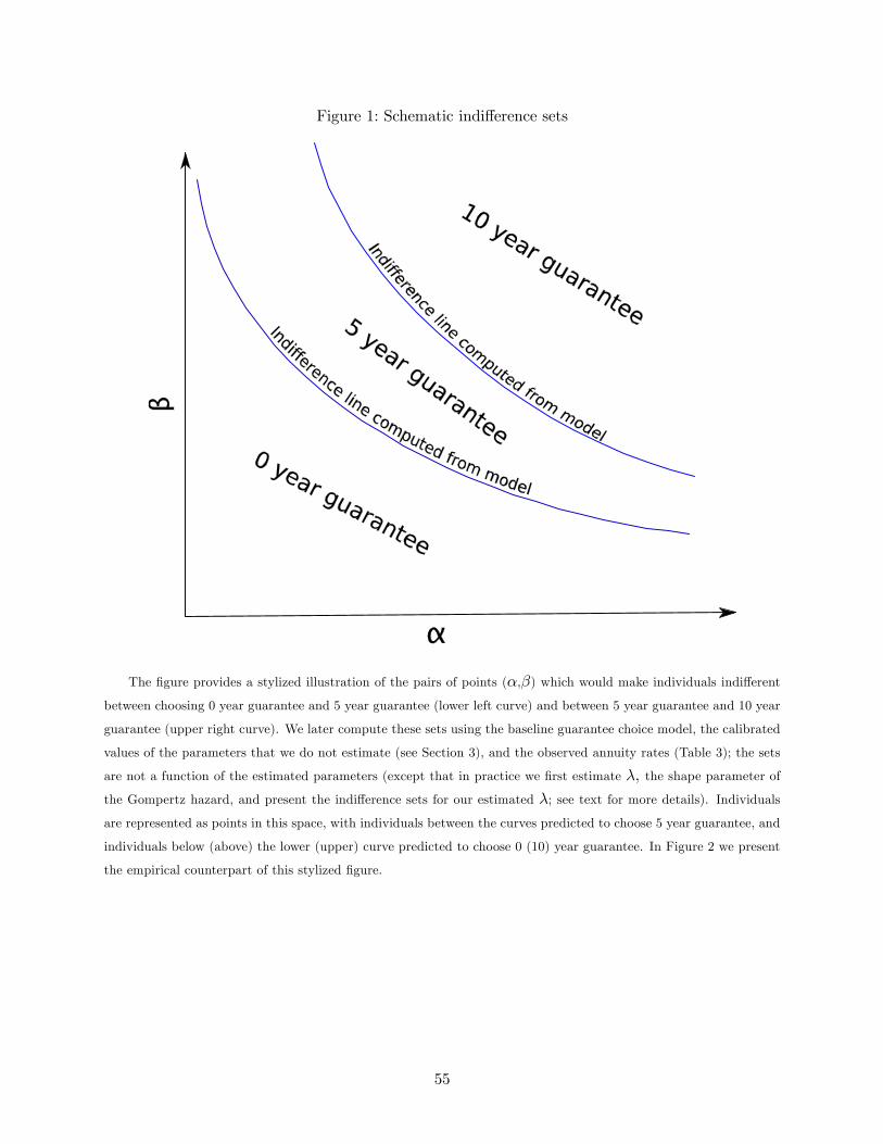
Figure 1: Schematic indifference sets

The figure provides a stylized illustration of the pairs of points (α,β) which would make individuals indifferent

between choosing 0 year guarantee and 5 year guarantee (lower left curve) and between 5 year guarantee and 10 year

guarantee (upper right curve). We later compute these sets using the baseline guarantee choice model, the calibrated

values of the parameters that we do not estimate (see Section 3), and the observed annuity rates (Table 3); the sets

are not a function of the estimated parameters (except that in practice we first estimate λ, the shape parameter of

the Gompertz hazard, and present the indifference sets for our estimated λ; see text for more details). Individuals

are represented as points in this space, with individuals between the curves predicted to choose 5 year guarantee, and

individuals below (above) the lower (upper) curve predicted to choose 0 (10) year guarantee. In Figure 2 we present

the empirical counterpart of this stylized figure.

55

Figure 2: Estimated distributions

60 Females

65 Females

65 Males

60 Males

The figure presents the estimated indifference sets, providing an empirical analog to Figure 1. It also presents

scatter plots from the estimated joint distribution of (logα,logβ); each point is a random draw from the estimated

distribution in the baseline specification. The estimated indifference sets for the 65 year old males are given by the

pair of dark dashed lines, for the 60 year old males by the pair of lighter dashed lines, for the 65 year old females by

the pair of dotted lines, and for the 60 year old females by the pair of solid lines.

56

Figure 3: Welfare contours

The figure super-imposes iso-welfare (wealth equivalent) contour lines on the previous Figure 2. Individuals with

wealth equivalent greater than 100 would voluntarily annuitize, while individuals with wealth equivalent less than

100 would not. Each panel represents a different age-gender cell: 60 year old females (upper left), 65 year old females

(upper right), 60 year old males (lower left), and 65 year old males (lower right).

57

Figure 4: Welfare change contours (symmetric information)

The figure presents Figure 2, with contour lines that present the change in welfare (wealth equivalent) from the

counterfactual exercise of symmetric information. Individuals with positive (negative) welfare change are estimated

to gain (lose) from symmetric information, compared to their welfare in the observed asymmetric information equi-

librium. Each panel represents a different age-gender cell: 60 year old females (upper left), 65 year old females (upper

right), 60 year old males (lower left), and 65 year old males (lower right).

58