The Weibull-Dagum Distribution: Properties and Applications

The Weibull-Dagum Distribution: Properties and Applications

M. H. TAHIR1, GAUSS M. CORDEIRO2, M. MANSOOR3 M. ZUBAIR4 ANDMORAD ALIZADEH5

1Department of Statistics, The Islamia University of Bahawalpur, PakistanEmail: [email protected]

2Department of Statistics, Federal University of Pernambuco, Recife, PE, Brazil3Department of Statistics, Punjab College, Bahawalpur, Pakistan

4Department of Statistics, Government Degree College, Kahrorpacca, Pakistan5Department of Statistics, Persian Gulf University of Bushehr, Bushehr, Iran

In this paper, we define a new lifetime model called the Weibull-Dagum distribution. The proposedmodel is based on the Weibull–G class (Bourguignon et al., 2014). It can also be defined by a sim-ple transformation of the Weibull random variable. Its density function is very flexible and can besymmetrical, left-skewed, right-skewed and reversed-J shaped. It has constant, increasing, decreas-ing, upside-down bathtub, bathtub and reversed-J shaped hazard rate. Various structural propertiesare derived including explicit expressions for the quantile function, ordinary and incomplete mo-ments and probability weighted moments. We also provide explicit expressions for the Renyi andq-entropies. We derive the density function of the order statistics as a mixture of Dagum densities.We use maximum likelihood to estimate the model parameters and illustrate the potentiality of thenew model by means of a simulation study and two applications to real data. In fact, the proposedmodel outperforms the beta-Dagum, McDonald-Dagum and Dagum models in these applications.

Keywords: Dagum distribution; Hazard function; Likelihood estimation; Moment; Weibull-Gfamily.

Mathematics Subject Classification (2010) 60E05; 62F10; 62N05

1. Introduction

There has been an increased interest in defining new generators of univariate continuous distri-butions by adding shape parameter(s) to the baseline distribution. This induction of parametershas been proved useful in exploring tail properties and also for improving the goodness-of-fit of thegenerated family. The well-known generators are the following: beta-G by Eugene et al. (2002) andJones (2004), Kumaraswamy-G (Kw-G) by Cordeiro and de Castro (2011), McDonald-G (Mc-G)by Alexander et al. (2012), gamma-X by Alzaatreh et al. (2013b), gamma-G (type 1) by Zografosand Balakrishanan (2009), gamma-G (type 2) by Ristic and Balakrishanan (2012), gamma-G (type3) by Torabi and Montazari (2012), log-gamma-G by Amini et al. (2014), logistic-G by Torabi and

1

Montazari (2014), exponentiated generalized-G by Cordeiro et al. (2013), transformed-transformer(T-X) family by Alzaatreh et al. (2013b), exponentiated T-X family by Alzaghal et al. (2013),Weibull-G by Bourguignon et al. (2014), exponentiated half-logistic-G by Cordeiro et al. (2014a),Lomax-G by Cordeiro et al. ( 2014b), T-X{Y} family (a quantile based approach) by Aljarrah etal. (2014), T-R{Y} family by Alzaatreh et al. (2014b), new Weibull-G by Tahir et al. (2014a) andlogistic-X by Tahir et al. (2014b).

Let r(t) be the probability density function (pdf) of a random variable T ∈ [a, b] for −∞ ≤ a <

b < ∞ and let W [G(x)] be a function of the cumulative distribution function (cdf) of a randomvariable X such that W [G(x)] satisfies the following conditions:

(i) W [G(x)] ∈ [a, b],

(ii) W [G(x)] is differentiable and monotonically non-decreasing, and

(iii) W [G(x)] → a as x → −∞ andW [G(x)] → b as x →∞.

(1)

Recently, Alzaatreh et al. (2013b) defined the T-X family of distributions by

F (x) =∫ W [G(x)]

ar(t) dt, (2)

where W [G(x)] satisfies the conditions (1). The pdf corresponding to (2) is given by

f(x) ={

d

dxW [G(x)]

}r {W [G(x)]} . (3)

In Table 1, we provide some W [G(x)] functions for special models of the T-X family.

Table 1: Some W [G(x)] functions for members of the T-X family

S.No. W[G(x)] Range of T Members of T-X family

1. G(x) [0, 1] Beta-G (Eugene et al., 2002)Kw-G type 1 (Cordeiro and de Castero, 2011)Mc-G (Alexander et al., 2012)Exp-G (Kw-G type 2) (Cordeiro et al., 2013)

2. - log [1−G(x)] (0,∞) Gamma-G Type-1 (Zografos and Balakrishanan, 2009)Log-Gamma-G Type-1 (Amini et al., 2014)Weibull-X (Alzaatreh et al., 2013a, 2013b)Gamma-X (Alzaatreh et al., 2012, 2013b, 2014a)Exponentiated Half-Logistic-G (Cordeiro et al., 2014a)Lomax-G (Cordeiro et al., 2014b)

3. - log [1−Gα(x)] (0,∞) Exponentiated T-X (Alzaghal et al., 2013)Exponentiated Weibull-X (Alzaghal et al., 2013)Exponentiated Gamma-X (Alzaghal et al., 2013)

4. G(x)1−G(x) (0,∞) Gamma-G Type-3 (Torabi and Montazri, 2012)

Weibull-G (Bourguignon et al., 2014)5. log

[ G(x)1−G(x)

](−∞,∞) Logistic-G (Torabi and Montazri, 2014)

6. log{- log [1−G(x)]} (−∞,∞) Logistic-X (Tahir et al., 2014b)

2

Camilo Dagum proposed a three-parameter (type I) and two four-parameter (type II and III)distributions for modeling size distribution of income in 1977 and 1980, respectively. However, theDagum type I (or Dagum) distribution has received increased attention just because of being atentative competitor as compared to other models. A detailed discussion on the Dagum distri-butions is addressed in Dagum (1983, 1990, 1996, 2006) and Kleiber (2008). In fact, the Dagummodel has many properties that are required for describing an income size model. The importanceof this model is that it provides good fit to the extreme sides of income data (Latorre, 1990). Itsapplications to human capital and personal income appeared in Costa (2006), Perez and Alaiz(2011), Ivana (2011), Lukasiewicz et al. (2012), Mala (2012) and Matejka and Duspivova (2013). Itwas also used for modeling tropospheric Ozone levels (Monroy et al., 2013), journals impact factors(Mishra, 2011), plant comet assay (Georgieva et al., 2010), tree inception voltage of silicon rubber(Ahmad et al., 2012) and breakdown voltage of unsaturated polyester resin (Ahmad et al., 2013).Aslam et al. (2011) proposed grouped acceptance sampling plans for the Dagum distribution underpercentile lifetimes. Binoti et al. (2012) and Alwan et al. (2013) worked with the Dagum distribu-tion for assessing the reliability of an electrical system and for describing diameter in teak standssubjected to thinning at different ages.

Kleiber and Kotz (2003), Kleiber (2008), Khan (2013), Shehzad and Asghar (2013) and Pant andHeadrick (2013) discussed properties and parameter estimation of the Dagum distribution. Domma(2007) determined the asymptotic distribution of the maximum likelihood estimators (MLEs) forthe right-truncated Dagum model. Pollastri and Zambruno (2010) proposed an estimation pro-cedure of the distribution of the ratio of two independent Dagum random variables. Domma etal. (2012) described the usefulness of the Dagum model in reliability theory and showed that itshazard rate function (hrf) can have a decreasing, an upside-down bathtub and a bathtub and thenupside-down bathtub forms. Domma et al. (2011a) discussed the maximum likelihood estimation ofthe Dagum’s parameters for censored data which usually occur in life-testing problems. The Fisherinformation matrix of doubly censored data, right censored data and type II doubly censored datawas computed in Domma et al. (2011b, 2013). Oluyede and Ye (2013) introduced the weightedDagum and related distributions.

Domma (2004) defined the log-Dagum distribution and studied the changes in the kurtosis byusing the kurtosis diagram given by Zenga (1996) and Polisicchio and Zenga (1997). Domma andPerri (2009) discussed some more structural properties and parameter estimation of the log-Dagumdistribution.

A random variable X has the Dagum distribution with three positive parameters λ, δ and β, ifits cdf is given by

Gλ,δ,β(x) = (1 + λx−δ)−β, x > 0, (4)

where λ is a scale parameter and δ and β are shape parameters. The pdf corresponding to (4) isgiven by

gλ,δ,β(x) = βλδ x−δ−1 (1 + λx−δ)−β−1, x > 0. (5)

The rth ordinary moment of X (for r ≤ δ) is determined from (5) as

µ′r = β λr/δ B(1− r

δ , β + rδ

), (6)

where B(p, q) =∫ 10 wp−1 (1− w)q−1dw is the complete beta function.

3

New ways of adding shape parameters to a baseline distribution have received increased atten-tion in recent years especially to explore tail properties of the transformed distributions. Thereexist only two such parameter inductions for the Dagum distribution which are based on the beta-Gand McDonald-G classes. First, Domma and Condino (2013) using the beta-G class (Eugene etal., 2002; Jones, 2004) extended the Dagum model by introducing two additional positive shapeparameters a and b whose role is to govern skewness and tail weights. The cdf and pdf of thefive-parameter beta-Dagum (BD) distribution are given by

F1(x; a, b, λ, δ, β) =1

B(a, b)

∫ Gλ,δ,β(x)

0wa−1 (1− w)b−1 dw = IGλ,δ,β(x)(a, b)

and

f1(x; a, b, λ, δ, β) =βλδ x−δ−1

B(a, b)

(1 + λx−δ

)−aβ−1[1−

(1 + λx−δ

)−β]b−1

,

where Iw(a, b) is the incomplete beta function ratio and Gλ,δ,β(x) is given by (4).Second, Oluyede and Rajasooriya (2013) adopted the McDonald-G class (Alexander et al., 2012)

to define the McDonald-Dagum (McD) distribution with six positive parameters. Its cdf and pdfare given by

F2(x; a, b, c, λ, δ, β) = IGcλ,δ,θ(x)(a, b) x > 0, a, b, c, λ, δ, β > 0,

and

f2(x; a, b, c, λ, δ, β) =cβλδ x−δ−1

B(a, b)

(1 + λx−δ

)−acβ−1[1−

(1 + λx−δ

)−cβ]b−1

,

respectively.Zagrafos and Balakrishnan (2009) pioneered a versatile and flexible gamma-G class of distri-

butions based on Stacy’s generalized gamma distribution and record value theory. More recently,Bourguignon et al. (2014) proposed the Weibull-G class of distributions influenced by the gamma-G class. Let G(x; Θ) and g(x; Θ) denote the cumulative and density functions of a baseline modelwith parameter vector Θ and the Weibull cdf ΠW (t) = 1−e−tb (for t > 0) with scale parameter oneand shape parameter b > 0. Bourguignon et al. (2014) replaced the argument t by G(t; Θ)/G(t; Θ),where G(t; Θ) = 1−G(t; Θ), and defined the cdf of their class, say Weibull-G(b, Θ), by

F (x) = F (x; b, Θ) = b

∫ hG(x;Θ)

G(x;Θ)

i

0tb−1 e−tb dt = 1− e

−h

G(x;Θ)

G(x;Θ)

ib, x ∈ <, b > 0. (7)

The use of odds G(x; Θ)/G(x; Θ) is an increasing function of x. Then, the Weibull-G pdf is givenby

f(x) = f(x; b, Θ) = b g(x; Θ)[G(x; Θ)b−1

G(x; Θ)b+1

]e−h

G(x;Θ)

G(x;Θ)

ib, x ∈ <, b > 0. (8)

It is noteworthy to mention that (7) is a special case of the T-X family (2) by taking W (G(x)) =G(x; Θ)/G(x; Θ) and r(t) as the corresponding Weibull pdf πW (t). The Weibull-G family does notprovide in general sub-models in the usual sense such as the beta-G, Kw-G and Mc-G familiessince the W [G(x)] function differs in both types of G-families. The Weibull-G family is based onW [G(x)] = G(x)/G(x) for unbounded interval (0,∞), whereas the three other families are based on

4

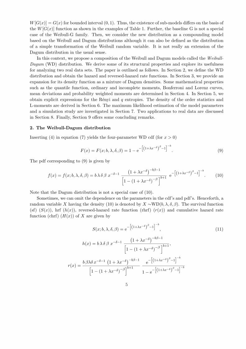
W [G(x)] = G(x) for bounded interval (0, 1). Thus, the existence of sub-models differs on the basis ofthe W [G(x)] function as shown in the examples of Table 1. Further, the baseline G is not a specialcase of the Weibull-G family. Then, we consider the new distribution as a compounding modelbased on the Weibull and Dagum distributions although it can also be defined as the distributionof a simple transformation of the Weibull random variable. It is not really an extension of theDagum distribution in the usual sense.

In this context, we propose a composition of the Weibull and Dagum models called the Weibull-Dagum (WD) distribution. We derive some of its structural properties and explore its usefulnessfor analyzing two real data sets. The paper is outlined as follows. In Section 2, we define the WDdistribution and obtain the hazard and reversed-hazard rate functions. In Section 3, we provide anexpansion for its density function as a mixture of Dagum densities. Some mathematical propertiessuch as the quantile function, ordinary and incomplete moments, Bonferroni and Lorenz curves,mean deviations and probability weighted moments are determined in Section 4. In Section 5, weobtain explicit expressions for the Renyi and q entropies. The density of the order statistics andL-moments are derived in Section 6. The maximum likelihood estimation of the model parametersand a simulation study are investigated in Section 7. Two applications to real data are discussedin Section 8. Finally, Section 9 offers some concluding remarks.

2. The Weibull-Dagum distribution

Inserting (4) in equation (7) yields the four-parameter WD cdf (for x > 0)

F (x) = F (x; b, λ, δ, β) = 1− e−h(1+λx−δ)β−1

i−b

. (9)

The pdf corresponding to (9) is given by

f(x) = f(x; b, λ, δ, β) = b λ δ β x−δ−1

(1 + λx−δ

)−bβ−1

[1− (1 + λx−δ)−β

]b+1e−h(1+λx−δ)β−1

i−b

. (10)

Note that the Dagum distribution is not a special case of (10).Sometimes, we can omit the dependence on the parameters in the cdf’s and pdf’s. Henceforth, a

random variable X having the density (10) is denoted by X ∼WD(b, λ, δ, β). The survival function(sf) (S(x)), hrf (h(x)), reversed-hazard rate function (rhrf) (r(x)) and cumulative hazard ratefunction (chrf) (H(x)) of X are given by

S(x; b, λ, δ, β) = e−h(1+λx−δ)β−1

i−b

, (11)

h(x) = b λ δ β x−δ−1

(1 + λx−δ

)−bβ−1

[1− (1 + λx−δ)−β

]b+1,

r(x) =b βλδ x−δ−1

(1 + λx−δ

)−bβ−1

[1− (1 + λx−δ)−β

]b+1

e−h(1+λx−δ)β−1

i−b

1− e−h(1+λx−δ)β−1

i−b

5

and

H(x) =[(

1 + λx−δ)β− 1

]−b

,

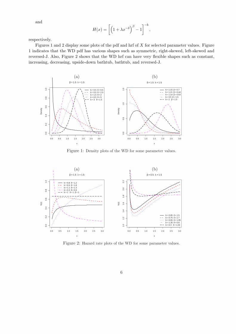
respectively.Figures 1 and 2 display some plots of the pdf and hrf of X for selected parameter values. Figure

1 indicates that the WD pdf has various shapes such as symmetric, right-skewed, left-skewed andreversed-J. Also, Figure 2 shows that the WD hrf can have very flexible shapes such as constant,increasing, decreasing, upside-down bathtub, bathtub, and reversed-J.

(a) (b)

0.0 0.5 1.0 1.5 2.0 2.5 3.0

0.0

0.2

0.4

0.6

0.8

1.0

β = 1.5 λ = 1.5

x

Den

sity

b = 0.5 δ = 0.5b = 0.5 δ = 2.5b = 1.5 δ = 2b = 0.5 δ = 5b = 3 δ = 1.5

0.0 0.5 1.0 1.5 2.0 2.5 3.0

0.0

0.5

1.0

1.5

δ = 1.5 λ = 1.5

x

Den

sity

b = 1.15 β = 0.7b = 1.21 β = 0.44b = 1.14 β = 0.53b = 3.5 β = 1.5b = 2 β = 1.5

Figure 1: Density plots of the WD for some parameter values.

(a) (b)

0.0 0.5 1.0 1.5 2.0 2.5 3.0

0.0

0.2

0.4

0.6

0.8

1.0

β = 1.5 λ = 1.5

x

h(x)

b = 0.8 δ = 1.2b = 0.5 δ = 1.8b = 1.1 δ = 1.3b = 0.3 δ = 0.9b = 1 δ = 1 β = 1

0.0 0.5 1.0 1.5 2.0 2.5 3.0

1.0

1.2

1.4

1.6

1.8

2.0

2.2

β = 0.5 λ = 1.5

x

h(x)

b = 0.85 δ = 1.5b = 0.75 δ = 1.7b = 0.65 δ = 1.95b = 1.35 δ = 0.8b = 0.3 δ = 1.03

Figure 2: Hazard rate plots of the WD for some parameter values.

6

Further, the limiting behavior of the hrf of X is

limx→0+

h(x) =

+∞; for b β δ < 1;

λ−1/δ; for b β δ = 1;

0; for b β δ > 1.

Lemma 1 provides some relations of the WD distribution with the well-known Weibull andexponential distributions.

Lemma 1 (Transformation): (a) If a random variable Y has the Weibull distribution with shapeparameter b > 0 and scale parameter one, then the random variable X =

{1λ

[(Y +1

Y )1/β − 1]}−1/δ

,where λ, δ and β are positive real numbers, follows the WD(b, λ, δ, β) distribution. (b) If a random

variable Y has the exponential distribution, then the random variable X ={

1λ

[(Y 1/b+1

Y 1/b

)1/β− 1

]}−1/δ

follows the WD(b, λ, δ, β) distribution.

3. Mixture Representation

By expanding the exponential function in (9) in power series, we obtain

F (x) = 1−∞∑

k=0

(−1)k

k!G(x)kb

G(x)kb=

∞∑

k=1

(−1)k+1

k!G(x)kb

G(x)kb.

Next, we use the expansion

(1− x)−ρ =∞∑

j=0

Γ(ρ + j) xj

j! Γ(ρ),

which holds for ρ > 0 and x ∈ (0, 1). Then,

F (x) =∞∑

k=1,j=0

(−1)k+1 Γ(kb + j)k! j! Γ(kb)

G(x)kb+j .

Let Hkb+j(x) = G(x)kb+j be the exponentiated-G (“exp-G” for short) distribution with powerparameter kb + j > 0. We have

F (x) =∞∑

k=1,j=0

vk,j Hkb+j(x), (12)

where the coefficients (for k ≥ 1, j ≥ 0) are given by

vk,j =(−1)k+1 Γ(kb + j)

k! j!Γ(kb)

and depend only on the generator parameter b.

7

By differentiating (12), we obtain

f(x) =∞∑

k=1,j=0

vk,j hkb+j(x), (13)

where hkb+j(x) is the exp-G density function with power parameter kb + j.

Using the Dagum cdf given in (4), we can rewrite (12) and (13) as

F (x) =∞∑

k=1,j=0

vk,j Gλ, δ, (kb+j)β(x). (14)

and

f(x) =∞∑

k=1,j=0

vk,j gλ, δ, (kb+j)β(x), (15)

where gλ, δ, (kb+j)β(x) denotes the Dagum pdf with parameters λ, δ and (kb + j)β.Equation (15) reveals that the WD density function is a mixture of Dagum densities. So,

several of the WD mathematical properties can be derived from those of the Dagum distribution.Equations (14) and (15) are the main results of this section.

4. Some Structural Properties

4.1Quantile Function and Simulation

Quantile functions are in widespread use in general statistics and often find representations in termsof lookup tables for key percentiles. The quantile function (qf) of the WD distribution is obtainedby inverting (9) as

QX(u) = λ1/δ

{[{1 +

(− log(1− u)

)−1/b}]1/β

− 1

}−1/δ

. (16)

The WD random variable is easily simulated. If U is a uniform variate on the unit interval (0, 1),then the random variable X = QX(U) follows (10), i.e. X ∼WD(b, λ, δ, β).

The analysis of the variability of the skewness and kurtosis on the shape parameters of X canbe investigated based on quantile measures. The Bowley skewness (Kenney and Keeping, 1962)based on quartiles is given by

B =Q(3/4) + Q(1/4)− 2Q(2/4)

Q(3/4)−Q(1/4).

The shortcomings of the classical kurtosis measure are well-known. The Moors kurtosis (Moors,1998) based on octiles is given by

M =Q(3/8)−Q(1/8) + Q(7/8)−Q(5/8)

Q(6/8)−Q(2/8).

8

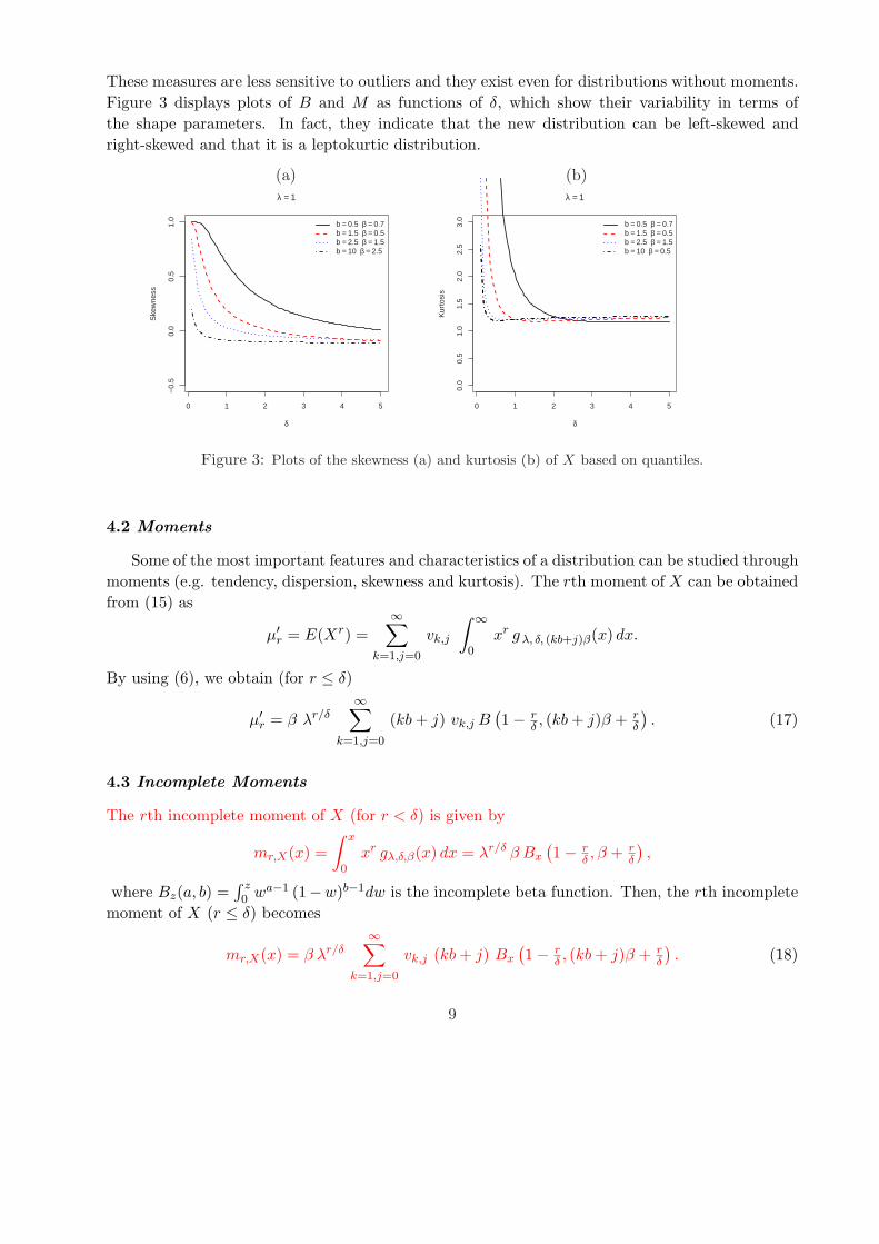
These measures are less sensitive to outliers and they exist even for distributions without moments.Figure 3 displays plots of B and M as functions of δ, which show their variability in terms ofthe shape parameters. In fact, they indicate that the new distribution can be left-skewed andright-skewed and that it is a leptokurtic distribution.

(a) (b)

0 1 2 3 4 5

−0.

50.

00.

51.

0

λ = 1

δ

Ske

wne

ss

b = 0.5 β = 0.7b = 1.5 β = 0.5b = 2.5 β = 1.5b = 10 β = 2.5

0 1 2 3 4 5

0.0

0.5

1.0

1.5

2.0

2.5

3.0

λ = 1

δ

Kur

tosi

s

b = 0.5 β = 0.7b = 1.5 β = 0.5b = 2.5 β = 1.5b = 10 β = 0.5

Figure 3: Plots of the skewness (a) and kurtosis (b) of X based on quantiles.

4.2 Moments

Some of the most important features and characteristics of a distribution can be studied throughmoments (e.g. tendency, dispersion, skewness and kurtosis). The rth moment of X can be obtainedfrom (15) as

µ′r = E(Xr) =∞∑

k=1,j=0

vk,j

∫ ∞

0xr gλ, δ, (kb+j)β(x) dx.

By using (6), we obtain (for r ≤ δ)

µ′r = β λr/δ∞∑

k=1,j=0

(kb + j) vk,j B(1− r

δ , (kb + j)β + rδ

). (17)

4.3 Incomplete Moments

The rth incomplete moment of X (for r < δ) is given by

mr,X(x) =∫ x

0xr gλ,δ,β(x) dx = λr/δ β Bx

(1− r

δ , β + rδ

),

where Bz(a, b) =∫ z0 wa−1 (1−w)b−1dw is the incomplete beta function. Then, the rth incomplete

moment of X (r ≤ δ) becomes

mr,X(x) = β λr/δ∞∑

k=1,j=0

vk,j (kb + j) Bx

(1− r

δ , (kb + j)β + rδ

). (18)

9

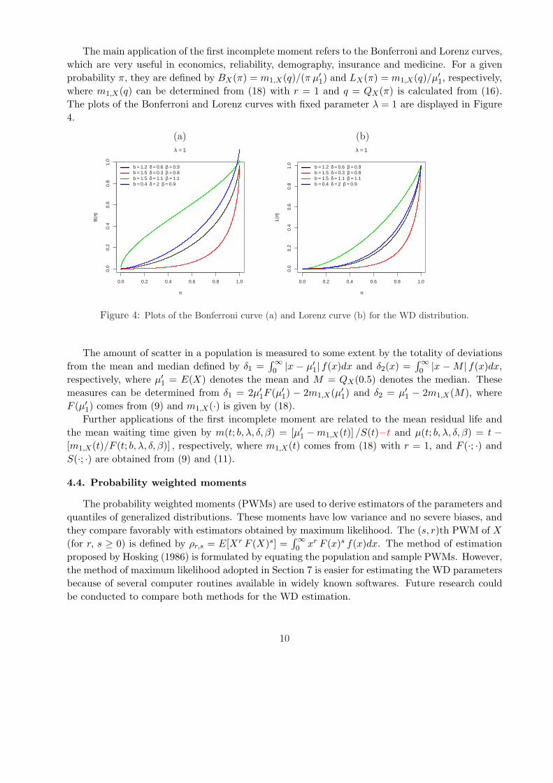
The main application of the first incomplete moment refers to the Bonferroni and Lorenz curves,which are very useful in economics, reliability, demography, insurance and medicine. For a givenprobability π, they are defined by BX(π) = m1,X(q)/(π µ′1) and LX(π) = m1,X(q)/µ′1, respectively,where m1,X(q) can be determined from (18) with r = 1 and q = QX(π) is calculated from (16).The plots of the Bonferroni and Lorenz curves with fixed parameter λ = 1 are displayed in Figure4.

(a) (b)

0.0 0.2 0.4 0.6 0.8 1.0

0.0

0.2

0.4

0.6

0.8

1.0

λ = 1

π

B(π

)

b = 1.2 δ = 0.6 β = 0.9b = 1.5 δ = 0.3 β = 0.8b = 1.5 δ = 1.1 β = 1.1b = 0.4 δ = 2 β = 0.9

0.0 0.2 0.4 0.6 0.8 1.0

0.0

0.2

0.4

0.6

0.8

1.0

λ = 1

π

L(π)

b = 1.2 δ = 0.6 β = 0.9b = 1.5 δ = 0.3 β = 0.8b = 1.5 δ = 1.1 β = 1.1b = 0.4 δ = 2 β = 0.9

Figure 4: Plots of the Bonferroni curve (a) and Lorenz curve (b) for the WD distribution.

The amount of scatter in a population is measured to some extent by the totality of deviationsfrom the mean and median defined by δ1 =

∫∞0 |x − µ′1| f(x)dx and δ2(x) =

∫∞0 |x − M | f(x)dx,

respectively, where µ′1 = E(X) denotes the mean and M = QX(0.5) denotes the median. Thesemeasures can be determined from δ1 = 2µ′1F (µ′1) − 2m1,X(µ′1) and δ2 = µ′1 − 2m1,X(M), whereF (µ′1) comes from (9) and m1,X(·) is given by (18).

Further applications of the first incomplete moment are related to the mean residual life andthe mean waiting time given by m(t; b, λ, δ, β) = [µ′1 −m1,X(t)] /S(t)−t and µ(t; b, λ, δ, β) = t −[m1,X(t)/F (t; b, λ, δ, β)] , respectively, where m1,X(t) comes from (18) with r = 1, and F (·; ·) andS(·; ·) are obtained from (9) and (11).

4.4. Probability weighted moments

The probability weighted moments (PWMs) are used to derive estimators of the parameters andquantiles of generalized distributions. These moments have low variance and no severe biases, andthey compare favorably with estimators obtained by maximum likelihood. The (s, r)th PWM of X

(for r, s ≥ 0) is defined by ρr,s = E[Xr F (X)s] =∫∞0 xr F (x)s f(x)dx. The method of estimation

proposed by Hosking (1986) is formulated by equating the population and sample PWMs. However,the method of maximum likelihood adopted in Section 7 is easier for estimating the WD parametersbecause of several computer routines available in widely known softwares. Future research couldbe conducted to compare both methods for the WD estimation.

10

By expanding the exponential function in (7) in power series, we have

F (x)s =∞∑

m=0

(−1)m

(s

m

)e−m

hG(x;Θ)

G(x;Θ)

ib.

Further, inserting the Weibull-G density (8) in F (x)s f(x) and using the exponential powerexpansion again, gives

F (x)s f(x) =∞∑

m=0

∞∑

k=0

(−1)m+k (m + 1)k

k!

(s

m

)b g(x; Θ) G(x; Θ)b(k+1)−1

× [1−G(x; Θ)]−[b(k+1)+1] .

Next, based on the binomial expansion (1 − x)−η =∑∞

j=0[Γ(η + j) xj ]/[j! Γ(η)], which holds forη > 0 and x ∈ (0, 1), we have

F (x)s f(x) =∞∑

m=0

∞∑

k=0

(−1)m+k (m + 1)k

k!

(s

m

)b g(x; Θ) G(x; Θ)b(k+1)−1

×∞∑

j=0

Γ(b(k + 1) + j + 1)G(x)j

j! Γ(b(k + 1) + 1)

and then

F (x)s f(x) =∞∑

m=0

∞∑

k,j=0

(s

m

)(−1)m+k (m + 1)k

k! j!b Γ(b(k + 1) + j)Γ(b(k + 1) + 1)

× [b(k + 1) + j] g(x; Θ) G(x; Θ)b(k+1)+j−1.

Using the pdf and cdf of the Dagum distribution in equations (4) and (5), we obtain

F (x)s f(x) =∞∑

k,j=0

qk,j,+ gλ,δ,[b(k+1)+j]β(x),

where

qk,j,+ =∞∑

m=0

(−1)m+k (m + 1)k

k! j!b Γ(b(k + 1) + j)Γ(b(k + 1) + 1)

(s

m

).

Further,

ρr,s =∞∑

k,j=0

qk,j,+

∫ ∞

0xr gλ,δ,[b(k+1)+j]β(x) dx.

Finally, we can express ρs,r (for r < δ) from (6) as

ρr,s = β λr/δ∞∑

k,j=0

qk,j,+ [b(k + 1) + j] B(1− r

δ , [b(k + 1) + j]β + rδ

). (19)

11

Equation (19) is the main result of this section.

5. The Renyi and q-entropies

The entropy of a random variable is a measure of the uncertainty variation. The Renyi entropy ofX is defined by

IR(θ) =1

1− θlog [I(θ)],

where I(θ) =∫< fθ(x) dx, θ > 0 and θ 6= 1.

Based on equation (8)

f(x)θ = bθ g(x)θ G(x)θ(b−1)

G(x)θ(b+1)e−θh

G(x)

G(x)

ib.

Using a power series for the exponential function and the generalized binomial expansion, we obtain

f(x)θ =∞∑

k,j=0

sk,j gθ(x) G(x)kb+θ(b−1)+j , (20)

where

sk,j =(−1)k θk bθ

k! j!Γ(kb + θ[b + 1] + j)

Γ(kb + θ[b + 1]).

Inserting (4) and (5) in equation (20), if follows that

I(θ) =∞∑

k,j=0

sk,j

∫ ∞

0(βλδ)θ x−θ(δ+1)

(1 + λx−δ

)−θ(β+1)−β[kb+θ(b−1)+j]dx.

For δ(α + 1) > 1 and δ(b− 1) > −1, transforming variables and integrating, I(θ) becomes

I(θ) =(βλδ)θ

δ λθ(δ+1)+1

δ

∞∑

k,j=0

sk,j B(θ(δ + 1)− 1

δ, θ(β + 1) + β[θ(b− 1) + bk + j]− θ(δ + 1)− 1

δ

). (21)

Hence, the Renyi entropy immediately comes from equation (21). The q-entropy, say Hq(f), isgiven by Hq(f) = (q − 1)−1 log [1− I(q)], where I(q) is determined from (21).

6. Order Statistics

Here, we provide the density of the ith order statistic Xi:n, fi:n(x) say, in a random sample of sizen from the WD distribution. By suppressing the parameters, we have (for i = 1, . . . , n)

fi:n(x) =f(x)

B(i, n− i + 1)

n−i∑

l=0

(−1)l(n−i

l

)F (x)i+l−1. (22)

Based on equation (7), we can write

F (x)i+l−1 =

[1− e

−h

G(x;Θ)

G(x;Θ)

ib]i+l−1

.

12

By expanding the exponential function in power series, we have

F (x)i+l−1 =∞∑

m=0

(−1)m

(i + l − 1

m

)e−m

hG(x;Θ)

G(x;Θ)

ib(23)

Based on equation (22), we obtain

fi:n(x) =1

B(i, n− i + 1)

n−i∑

l=0

∞∑

m=0

(−1)l+m b

(n− i

l

)(i + l − 1

m

)

× g(x; Θ)G(x; Θ)b−1

G(x; Θ)b+1e−(m+1)

hG(x;Θ)

G(x;Θ)

ib.

By using the power series for the exponential function again, we have

fi:n(x) =1

B(i, n− i + 1)

n−i∑

l=0

∞∑

k,m=0

(−1)l+m+k b (m + 1)k

k!

(n− i

l

)(i + l − 1

m

)

× g(x; Θ)G(x; Θ)b(k+1)+j−1

G(x; Θ)b(k+1)+j+1.

Based on the expansion

(1− x)−η =∞∑

j=0

Γ(η + j) xj

j! Γ(η),

which holds for η > 0 and x ∈ (0, 1), we can write

fi:n(x) =1

B(i, n− i + 1)

n−i∑

l=0

∞∑

k,m=0

(−1)l+m+k b (m + 1)k

k!

(n− i

l

)(i + l − 1

m

)

× g(x; Θ) G(x; Θ)b(k+1)−1∞∑

j=0

Γ(b(k + 1) + j + 1)G(x)j

j! Γ(b(k + 1) + 1),

and then

fi:n(x) =∞∑

k,j=0

wk,j [b(k + 1) + j] g(x; Θ) G(x; Θ)b(k+1)+j−1,

where

wk,j =n−i∑

l=0

∞∑

m=0

(−1)l+m+k b (m + 1)k

k! j!

(n− i

l

)(i + l − 1

m

)Γ(b(k + 1) + j)Γ(b(k + 1) + 1)

.

Finally, using the pdf (5) and cdf (4) of the Dagum distribution, we obtain

fi:n(x) =∞∑

k,j=0

wk,j gλ,δ,[b(k+1)+j]β(x). (24)

13

Equation (24) reveals that the density function of the WD order statistics is a linear combination ofthe Dagum densities. So, we can easily obtain the mathematical properties for Xi:n. For example,the rth moment of Xi:n follows from (6) and (24) (for r ≤ δ) as

E(Xri:n) = β λr/δ

∞∑

k,j=0

wk,j [b(k + 1) + j]B(1− r

δ , [b(k + 1) + j]β + rδ

), (25)

where

wk,j =n−i∑

l=0

∞∑

m=0

(−1)l+m+k b (m + 1)k

k! j!

(n− i

l

)(i + l − 1

m

)Γ(b(k + 1) + j)Γ(b(k + 1) + 1)

.

The L-moments are analogous to the ordinary moments but can be estimated by linear combi-nations of order statistics. They exist whenever the mean of the distribution exists, even thoughsome higher moments may not exist, and are relatively robust to the effects of outliers. Basedupon the moments (25), we can derive explicit expressions for the L-moments of X as infiniteweighted linear combinations of the means of suitable WD distributions. They are linear functionsof expected order statistics defined by (for s ≥ 1) λs = s−1

∑s−1p=0(−1)p

(s−1p

)E(Xs−p:p). The first

four L-moments are: λ1 = E(X1:1), λ2 = 12E(X2:2 − X1:2), λ3 = 1

3E(X3:3 − 2X2:3 + X1:3) andλ4 = 1

4E(X4:4 − 3X3:4 + 3X2:4 − X1:4). We can easily obtain λs for X from equation (25) withr = 1.

7. Estimation

Inference can be carried out in three different ways: point estimation, interval estimation and hy-pothesis testing. Several approaches for parameter point estimation were proposed in the literaturebut the maximum likelihood method is the most commonly employed. The MLEs enjoy desirableproperties and can be used when constructing confidence intervals and regions and also in teststatistics. Large sample theory for these estimates delivers simple approximations that work wellin finite samples. Statisticians often seek to approximate quantities such as the density of a teststatistic that depend on the sample size in order to obtain better approximate distributions. Theresulting approximation for the MLEs in distribution theory is easily handled either analyticallyor numerically. So, we consider the estimation of the unknown parameters of the WD distributionby the method of maximum likelihood. Let x1, . . . , xn be a random sample of size n from the WDdistribution given by (10). The log-likelihood function for the vector of parameters Θ = (b, λ, δ, β)>

can be expressed as

` = `(Θ) = n log (b λ δ β)− (δ + 1)n∑

i=1

log xi − (bβ + 1)n∑

i=1

log(1 + λx−δ

i

)

−(b + 1)n∑

i=1

log[1−

(1 + λx−δ

i

)−β]−

n∑

i=1

[(1 + λx−δ

i

)β− 1

]−b

.

Let zi = (1 + λx−δi ). We have

∂ zi

∂λ= z′iλ = x−δ

i ,∂ zi

∂δ= z′iδ = −λx−δ

i log xi ,∂2 zi

(∂λ)2= z′′iλ = 0 ,

∂2 zi

(∂δ)2= z′′iδ = λx−δ

i (log xi)2 ,

14

and∂2 zi

∂λ∂δ= z′′iλ = −x−δ

i log xi.

Then, we can write ` = `(Θ) as

` = n log (b λ δ β)− (δ + 1)n∑

i=1

log xi − (b β + 1)n∑

i=1

log zi

− (b + 1)n∑

i=1

log(1− z−β

i

)−

n∑

i=1

(zβi − 1

)−b.

The components of the score vector U(Θ) are given by

Ub(Θ) =n

b− β

n∑

i=1

log zi −n∑

i=1

log(1− z−β

i

)+

n∑

i=1

(zβi − 1

)−blog

(zβi − 1

),

Uλ(Θ) =n

λ− (bβ + 1)

n∑

i=1

(z′iλzi

)− β(b + 1)

n∑

i=1

(z−β−1i z′iλ1− z−β

i

)

+bβn∑

i=1

(zβi − 1

)−b−1zβ−1i z′iλ ,

Uδ(Θ) =n

δ−

n∑

i=1

log xi − (bβ + 1)n∑

i=1

(z′iδzi

)− β(b + 1)

n∑

i=1

(z−β−1i z′iδ1− z−β

i

)

+bβn∑

i=1

(zβi − 1

)−b−1zβ−1i z′iδ ,

Uβ(Θ) =n

β− b

n∑

i=1

log zi − (b + 1)n∑

i=1

(z−βi log zi

1− z−βi

)

+bn∑

i=1

(zβi − 1

)−b−1zβi log zi .

The MLEs of the model parameters are determined from the solutions of the nonlinear equationsU(Θ) = 0, which can be solved iteratively.

For interval estimation of the parameters, we require the 4 × 4 observed information matrixJ(Θ) = {Jrs} (for r, s = b, λ, δ, β), whose elements are given in Appendix A. Under standard reg-ularity conditions, the multivariate normal N4(0, J(Θ)−1) distribution can be used to constructapproximate confidence intervals for the parameters in Θ. Here, J(Θ) is the total observed infor-mation matrix evaluated at Θ. Then, the 100(1 − γ)% confidence intervals for b, λ, δ and β are

given by b ± zγ/2 ×√

var(b), λ ± zγ/2 ×√

var(λ), δ ± zγ/2 ×√

var(δ) and β ± zγ/2 ×√

var(β),

respectively, where var(·)’s denote the diagonal elements of J(Θ)−1 corresponding to the modelparameters, and zγ/2 is the quantile (1− γ/2) of the standard normal distribution.

15

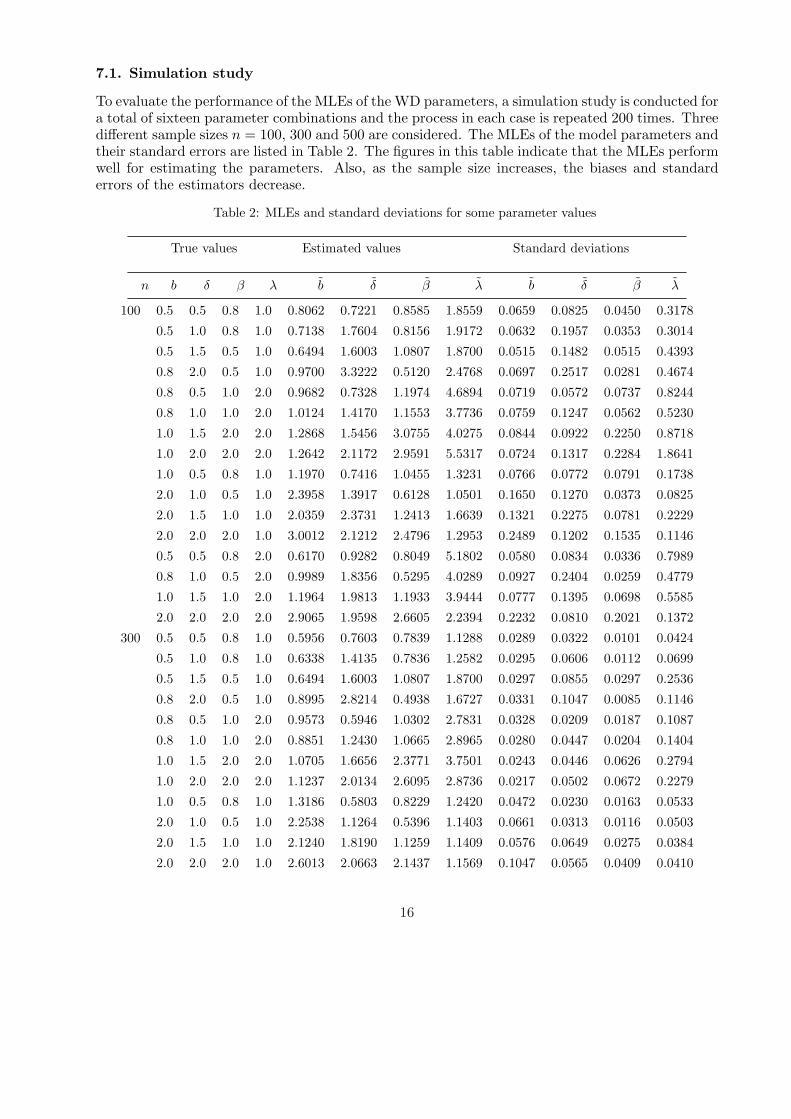
7.1. Simulation study

To evaluate the performance of the MLEs of the WD parameters, a simulation study is conducted fora total of sixteen parameter combinations and the process in each case is repeated 200 times. Threedifferent sample sizes n = 100, 300 and 500 are considered. The MLEs of the model parameters andtheir standard errors are listed in Table 2. The figures in this table indicate that the MLEs performwell for estimating the parameters. Also, as the sample size increases, the biases and standarderrors of the estimators decrease.

Table 2: MLEs and standard deviations for some parameter values

True values Estimated values Standard deviations

n b δ β λ b δ β λ b δ β λ

100 0.5 0.5 0.8 1.0 0.8062 0.7221 0.8585 1.8559 0.0659 0.0825 0.0450 0.3178

0.5 1.0 0.8 1.0 0.7138 1.7604 0.8156 1.9172 0.0632 0.1957 0.0353 0.3014

0.5 1.5 0.5 1.0 0.6494 1.6003 1.0807 1.8700 0.0515 0.1482 0.0515 0.4393

0.8 2.0 0.5 1.0 0.9700 3.3222 0.5120 2.4768 0.0697 0.2517 0.0281 0.4674

0.8 0.5 1.0 2.0 0.9682 0.7328 1.1974 4.6894 0.0719 0.0572 0.0737 0.8244

0.8 1.0 1.0 2.0 1.0124 1.4170 1.1553 3.7736 0.0759 0.1247 0.0562 0.5230

1.0 1.5 2.0 2.0 1.2868 1.5456 3.0755 4.0275 0.0844 0.0922 0.2250 0.8718

1.0 2.0 2.0 2.0 1.2642 2.1172 2.9591 5.5317 0.0724 0.1317 0.2284 1.8641

1.0 0.5 0.8 1.0 1.1970 0.7416 1.0455 1.3231 0.0766 0.0772 0.0791 0.1738

2.0 1.0 0.5 1.0 2.3958 1.3917 0.6128 1.0501 0.1650 0.1270 0.0373 0.0825

2.0 1.5 1.0 1.0 2.0359 2.3731 1.2413 1.6639 0.1321 0.2275 0.0781 0.2229

2.0 2.0 2.0 1.0 3.0012 2.1212 2.4796 1.2953 0.2489 0.1202 0.1535 0.1146

0.5 0.5 0.8 2.0 0.6170 0.9282 0.8049 5.1802 0.0580 0.0834 0.0336 0.7989

0.8 1.0 0.5 2.0 0.9989 1.8356 0.5295 4.0289 0.0927 0.2404 0.0259 0.4779

1.0 1.5 1.0 2.0 1.1964 1.9813 1.1933 3.9444 0.0777 0.1395 0.0698 0.5585

2.0 2.0 2.0 2.0 2.9065 1.9598 2.6605 2.2394 0.2232 0.0810 0.2021 0.1372

300 0.5 0.5 0.8 1.0 0.5956 0.7603 0.7839 1.1288 0.0289 0.0322 0.0101 0.0424

0.5 1.0 0.8 1.0 0.6338 1.4135 0.7836 1.2582 0.0295 0.0606 0.0112 0.0699

0.5 1.5 0.5 1.0 0.6494 1.6003 1.0807 1.8700 0.0297 0.0855 0.0297 0.2536

0.8 2.0 0.5 1.0 0.8995 2.8214 0.4938 1.6727 0.0331 0.1047 0.0085 0.1146

0.8 0.5 1.0 2.0 0.9573 0.5946 1.0302 2.7831 0.0328 0.0209 0.0187 0.1087

0.8 1.0 1.0 2.0 0.8851 1.2430 1.0665 2.8965 0.0280 0.0447 0.0204 0.1404

1.0 1.5 2.0 2.0 1.0705 1.6656 2.3771 3.7501 0.0243 0.0446 0.0626 0.2794

1.0 2.0 2.0 2.0 1.1237 2.0134 2.6095 2.8736 0.0217 0.0502 0.0672 0.2279

1.0 0.5 0.8 1.0 1.3186 0.5803 0.8229 1.2420 0.0472 0.0230 0.0163 0.0533

2.0 1.0 0.5 1.0 2.2538 1.1264 0.5396 1.1403 0.0661 0.0313 0.0116 0.0503

2.0 1.5 1.0 1.0 2.1240 1.8190 1.1259 1.1409 0.0576 0.0649 0.0275 0.0384

2.0 2.0 2.0 1.0 2.6013 2.0663 2.1437 1.1569 0.1047 0.0565 0.0409 0.0410

16

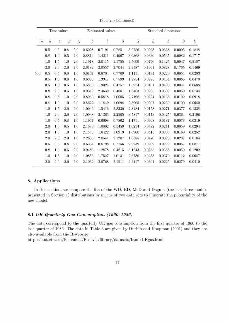
Table 2: (Continued)

True values Estimated values Standard deviations

n b δ β λ b δ β λ b δ β λ

0.5 0.5 0.8 2.0 0.6028 0.7191 0.7851 3.2756 0.0263 0.0338 0.0095 0.1848

0.8 1.0 0.5 2.0 0.8814 1.4211 0.4967 3.0368 0.0330 0.0535 0.0082 0.1717

1.0 1.5 1.0 2.0 1.1918 2.0115 1.1755 4.5699 0.0746 0.1425 0.0947 0.5187

2.0 2.0 2.0 2.0 2.6182 2.0557 2.7044 2.2587 0.1901 0.0828 0.1765 0.1469

500 0.5 0.5 0.8 1.0 0.6167 0.6704 0.7769 1.1111 0.0194 0.0220 0.0054 0.0283

0.5 1.0 0.8 1.0 0.6386 1.3347 0.7599 1.2754 0.0225 0.0454 0.0065 0.0470

0.5 1.5 0.5 1.0 0.5850 1.9024 0.4757 1.5274 0.0161 0.0490 0.0044 0.0688

0.8 2.0 0.5 1.0 0.9349 2.4639 0.4861 1.6483 0.0235 0.0609 0.0059 0.0734

0.8 0.5 1.0 2.0 0.8960 0.5818 1.0005 2.7198 0.0224 0.0136 0.0102 0.0918

0.8 1.0 1.0 2.0 0.8622 1.1849 1.0098 2.5965 0.0207 0.0269 0.0100 0.0680

1.0 1.5 2.0 2.0 1.0946 1.5416 2.3330 2.8484 0.0158 0.0271 0.0377 0.1338

1.0 2.0 2.0 2.0 1.0938 2.1363 2.2505 3.5817 0.0173 0.0425 0.0364 0.2196

1.0 0.5 0.8 1.0 1.1967 0.6098 0.7862 1.1751 0.0308 0.0187 0.0078 0.0319

2.0 1.0 0.5 1.0 2.1683 1.0802 0.5459 1.0254 0.0482 0.0211 0.0059 0.0294

2.0 1.5 1.0 1.0 2.1546 1.6422 1.0919 1.0900 0.0415 0.0305 0.0169 0.0252

2.0 2.0 2.0 1.0 2.2606 2.0541 2.1207 1.0585 0.0470 0.0323 0.0237 0.0184

0.5 0.5 0.8 2.0 0.6364 0.6798 0.7756 2.9239 0.0209 0.0229 0.0057 0.0877

0.8 1.0 0.5 2.0 0.9483 1.2878 0.4815 3.1243 0.0253 0.0366 0.0059 0.1202

1.0 1.5 1.0 2.0 1.0856 1.7527 1.0131 2.6736 0.0253 0.0370 0.0112 0.0687

2.0 2.0 2.0 2.0 2.1032 2.0768 2.1511 2.2117 0.0391 0.0225 0.0279 0.0410

8. Applications

In this section, we compare the fits of the WD, BD, McD and Dagum (the last three modelspresented in Section 1) distributions by means of two data sets to illustrate the potentiality of thenew model.

8.1 UK Quarterly Gas Consumption (1960–1986)

The data correspond to the quarterly UK gas consumption from the first quarter of 1960 to thelast quarter of 1986. The data in Table 3 are given by Durbin and Koopman (2001) and they arealso available from the R-websitehttp://stat.ethz.ch/R-manual/R-devel/library/datasets/html/UKgas.html

17

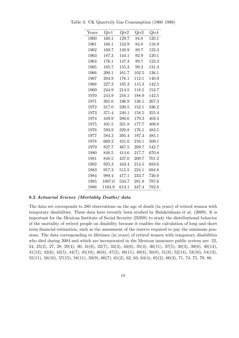
Table 3: UK Quarterly Gas Consumption (1960–1986)

Years Qtr1 Qtr2 Qtr3 Qtr41960 160.1 129.7 84.8 120.11961 160.1 124.9 84.8 116.91962 169.7 140.9 89.7 123.31963 187.3 144.1 92.9 120.11964 176.1 147.3 89.7 123.31965 185.7 155.3 99.3 131.31966 200.1 161.7 102.5 136.11967 204.9 176.1 112.1 140.91968 227.3 195.3 115.3 142.51969 244.9 214.5 118.5 153.71970 244.9 216.1 188.9 142.51971 301.0 196.9 136.1 267.31972 317.0 230.5 152.1 336.21973 371.4 240.1 158.5 355.41974 449.9 286.6 179.3 403.41975 491.5 321.8 177.7 409.81976 593.9 329.8 176.1 483.51977 584.3 395.4 187.3 485.11978 669.2 421.0 216.1 509.11979 827.7 467.5 209.7 542.71980 840.5 414.6 217.7 670.81981 848.5 437.0 209.7 701.21982 925.3 443.4 214.5 683.61983 917.3 515.5 224.1 694.81984 989.4 477.1 233.7 730.01985 1087.0 534.7 281.8 787.61986 1163.9 613.1 347.4 782.8

8.2 Actuarial Science (Mortality Deaths) data

The data set corresponds to 280 observations on the age of death (in years) of retired women withtemporary disabilities. These data have recently been studied by Balakrishnan et al. (2009). It isimportant for the Mexican Institute of Social Security (IMSS) to study the distributional behaviorof the mortality of retired people on disability because it enables the calculation of long and shortterm financial estimation, such as the assessment of the reserve required to pay the minimum pen-sions. The data corresponding to lifetimes (in years) of retired women with temporary disabilitieswho died during 2004 and which are incorporated in the Mexican insurance public system are: 22,24, 25(2), 27, 28, 29(4), 30, 31(6), 32(7), 33(3), 34(6), 35(4), 36(11), 37(5), 38(3), 39(6), 40(14),41(12), 42(6), 43(5), 44(7), 45(10), 46(6), 47(5), 48(11), 49(8), 50(8), 51(8), 52(14), 53(10), 54(13),55(11), 56(10), 57(15), 58(11), 59(9), 60(7), 61(2), 62, 63, 64(4), 65(2), 66(3), 71, 74, 75, 79, 86.

18

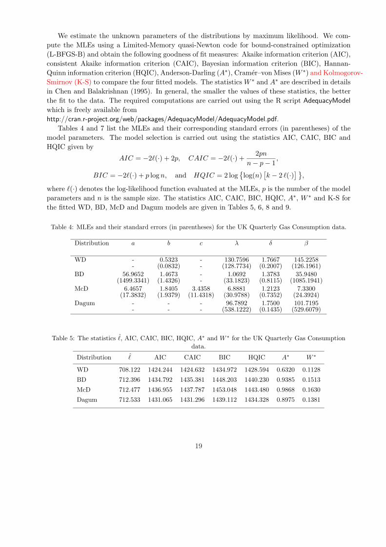
We estimate the unknown parameters of the distributions by maximum likelihood. We com-pute the MLEs using a Limited-Memory quasi-Newton code for bound-constrained optimization(L-BFGS-B) and obtain the following goodness of fit measures: Akaike information criterion (AIC),consistent Akaike information criterion (CAIC), Bayesian information criterion (BIC), Hannan-Quinn information criterion (HQIC), Anderson-Darling (A∗), Cramer–von Mises (W ∗) and Kolmogorov-Smirnov (K-S) to compare the four fitted models. The statistics W ∗ and A∗ are described in detailsin Chen and Balakrishnan (1995). In general, the smaller the values of these statistics, the betterthe fit to the data. The required computations are carried out using the R script AdequacyModel

which is freely available fromhttp://cran.r-project.org/web/packages/AdequacyModel/AdequacyModel.pdf.

Tables 4 and 7 list the MLEs and their corresponding standard errors (in parentheses) of themodel parameters. The model selection is carried out using the statistics AIC, CAIC, BIC andHQIC given by

AIC = −2`(·) + 2p, CAIC = −2`(·) +2pn

n− p− 1,

BIC = −2`(·) + p logn, and HQIC = 2 log{log(n)

[k − 2 `(·)] }

,

where `(·) denotes the log-likelihood function evaluated at the MLEs, p is the number of the modelparameters and n is the sample size. The statistics AIC, CAIC, BIC, HQIC, A∗, W ∗ and K-S forthe fitted WD, BD, McD and Dagum models are given in Tables 5, 6, 8 and 9.

Table 4: MLEs and their standard errors (in parentheses) for the UK Quarterly Gas Consumption data.

Distribution a b c λ δ β

WD - 0.5323 - 130.7596 1.7667 145.2258- (0.0832) - (128.7734) (0.2007) (126.1961)

BD 56.9652 1.4673 - 1.0692 1.3783 35.9480(1499.3341) (1.4326) - (33.1823) (0.8115) (1085.1941)

McD 6.4657 1.8405 3.4358 6.8881 1.2123 7.3300(17.3832) (1.9379) (11.4318) (30.9788) (0.7352) (24.3924)

Dagum - - - 96.7892 1.7500 101.7195- - - (538.1222) (0.1435) (529.6079)

Table 5: The statistics ˆ, AIC, CAIC, BIC, HQIC, A∗ and W ∗ for the UK Quarterly Gas Consumptiondata.

Distribution ˆ AIC CAIC BIC HQIC A∗ W ∗

WD 708.122 1424.244 1424.632 1434.972 1428.594 0.6320 0.1128

BD 712.396 1434.792 1435.381 1448.203 1440.230 0.9385 0.1513

McD 712.477 1436.955 1437.787 1453.048 1443.480 0.9868 0.1630

Dagum 712.533 1431.065 1431.296 1439.112 1434.328 0.8975 0.1381

19

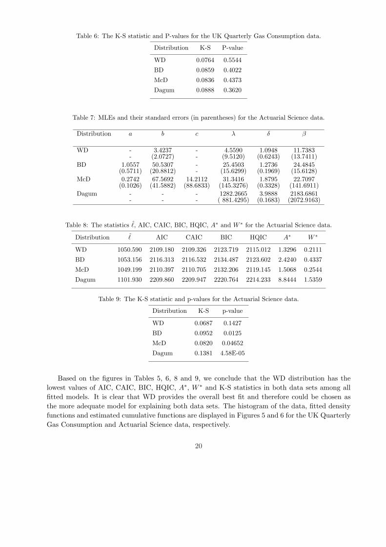
Table 6: The K-S statistic and P-values for the UK Quarterly Gas Consumption data.

Distribution K-S P-value

WD 0.0764 0.5544

BD 0.0859 0.4022

McD 0.0836 0.4373

Dagum 0.0888 0.3620

Table 7: MLEs and their standard errors (in parentheses) for the Actuarial Science data.

Distribution a b c λ δ β

WD - 3.4237 - 4.5590 1.0948 11.7383- (2.0727) - (9.5120) (0.6243) (13.7411)

BD 1.0557 50.5307 - 25.4503 1.2736 24.4845(0.5711) (20.8812) - (15.6299) (0.1969) (15.6128)

McD 0.2742 67.5692 14.2112 31.3416 1.8795 22.7097(0.1026) (41.5882) (88.6833) (145.3276) (0.3328) (141.6911)

Dagum - - - 1282.2665 3.9888 2183.6861- - - ( 881.4295) (0.1683) (2072.9163)

Table 8: The statistics ˆ, AIC, CAIC, BIC, HQIC, A∗ and W ∗ for the Actuarial Science data.

Distribution ˆ AIC CAIC BIC HQIC A∗ W ∗

WD 1050.590 2109.180 2109.326 2123.719 2115.012 1.3296 0.2111

BD 1053.156 2116.313 2116.532 2134.487 2123.602 2.4240 0.4337

McD 1049.199 2110.397 2110.705 2132.206 2119.145 1.5068 0.2544

Dagum 1101.930 2209.860 2209.947 2220.764 2214.233 8.8444 1.5359

Table 9: The K-S statistic and p-values for the Actuarial Science data.

Distribution K-S p-value

WD 0.0687 0.1427

BD 0.0952 0.0125

McD 0.0820 0.04652

Dagum 0.1381 4.58E-05

Based on the figures in Tables 5, 6, 8 and 9, we conclude that the WD distribution has thelowest values of AIC, CAIC, BIC, HQIC, A∗, W ∗ and K-S statistics in both data sets among allfitted models. It is clear that WD provides the overall best fit and therefore could be chosen asthe more adequate model for explaining both data sets. The histogram of the data, fitted densityfunctions and estimated cumulative functions are displayed in Figures 5 and 6 for the UK QuarterlyGas Consumption and Actuarial Science data, respectively.

20

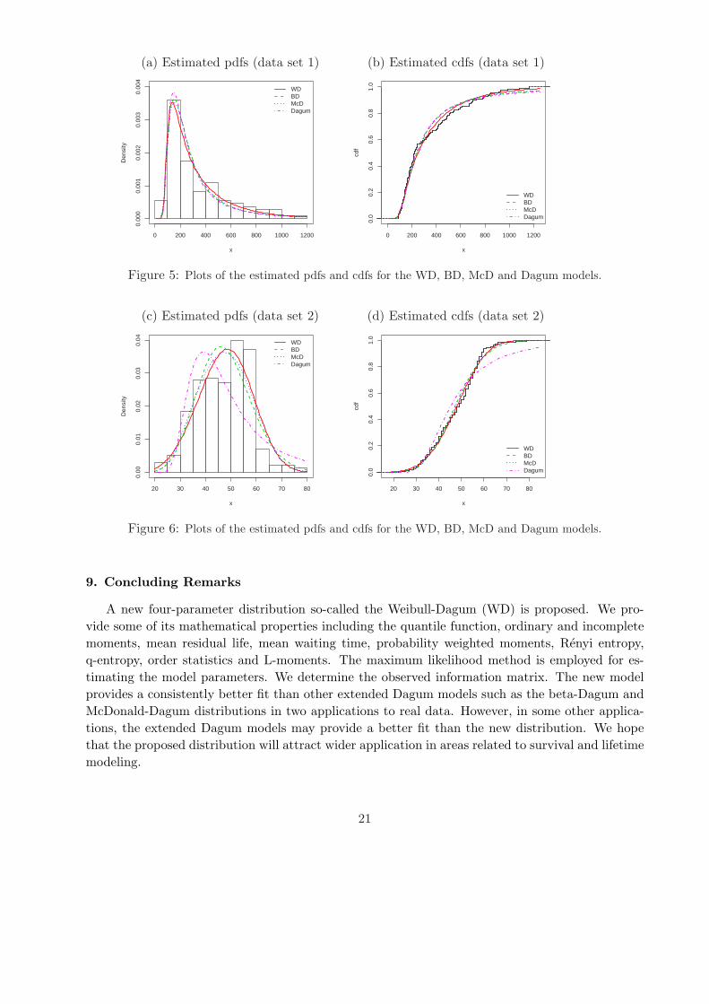
(a) Estimated pdfs (data set 1) (b) Estimated cdfs (data set 1)

x

Den

sity

0 200 400 600 800 1000 1200

0.00

00.

001

0.00

20.

003

0.00

4

WDBDMcDDagum

0 200 400 600 800 1000 1200

0.0

0.2

0.4

0.6

0.8

1.0

x

cdf

WDBDMcDDagum

Figure 5: Plots of the estimated pdfs and cdfs for the WD, BD, McD and Dagum models.

(c) Estimated pdfs (data set 2) (d) Estimated cdfs (data set 2)

x

Den

sity

20 30 40 50 60 70 80

0.00

0.01

0.02

0.03

0.04 WD

BDMcDDagum

20 30 40 50 60 70 80

0.0

0.2

0.4

0.6

0.8

1.0

x

cdf

WDBDMcDDagum

Figure 6: Plots of the estimated pdfs and cdfs for the WD, BD, McD and Dagum models.

9. Concluding Remarks

A new four-parameter distribution so-called the Weibull-Dagum (WD) is proposed. We pro-vide some of its mathematical properties including the quantile function, ordinary and incompletemoments, mean residual life, mean waiting time, probability weighted moments, Renyi entropy,q-entropy, order statistics and L-moments. The maximum likelihood method is employed for es-timating the model parameters. We determine the observed information matrix. The new modelprovides a consistently better fit than other extended Dagum models such as the beta-Dagum andMcDonald-Dagum distributions in two applications to real data. However, in some other applica-tions, the extended Dagum models may provide a better fit than the new distribution. We hopethat the proposed distribution will attract wider application in areas related to survival and lifetimemodeling.

21

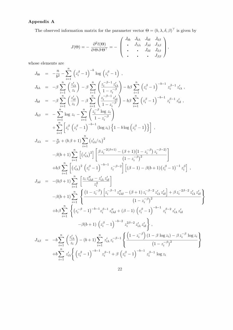
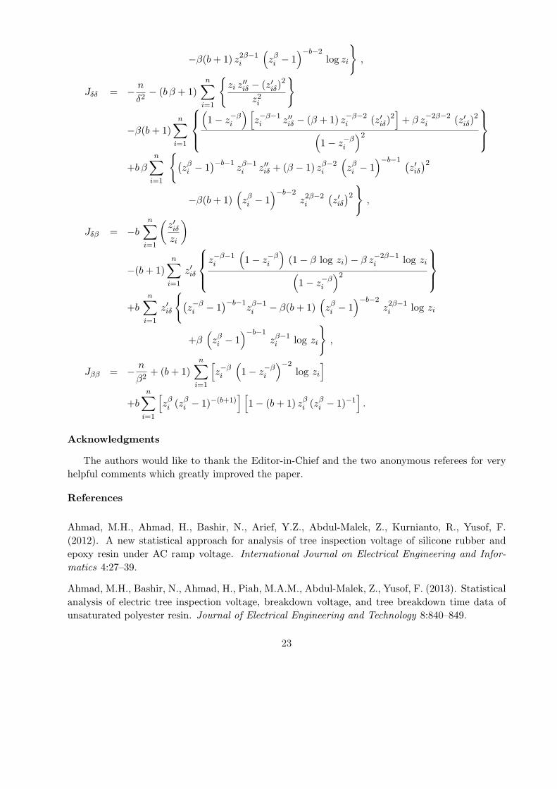
Appendix A

The observed information matrix for the parameter vector Θ = (b, λ, δ, β)> is given by

J(Θ) = − ∂2`(Θ)∂ Θ ∂ Θ> = −

Jbb Jbλ Jbδ Jbβ

¦ Jλλ Jλδ Jλβ

¦ ¦ Jδδ Jδβ

¦ ¦ ¦ Jββ

,

whose elements are

Jbb = − n

b2−

n∑

i=1

(zβi − 1

)−blog

(zβi − 1

),

Jbλ = −βn∑

i=1

(z′iλzi

)− β

n∑

i=1

(z−β−1i z′iλ1− z−β

i

)− bβ

n∑

i=1

(zβi − 1

)−b−1zβ−1i z′iλ ,

Jbδ = −β

n∑

i=1

(z′iδzi

)− β

n∑

i=1

(z−β−1i z′iδ1− z−β

i

)− bβ

n∑

i=1

(zβi − 1

)−b−1zβ−1i z′iδ ,

Jbβ = −n∑

i=1

log zi −n∑

i=1

(z−βi log zi

1− z−βi

)

+n∑

i=1

[zβi

(zβi − 1

)−b−1(log zi)

{1− b log

(zβi − 1

)}],

Jλλ = − nλ2 + (b β + 1)

n∑

i=1

(z′iλ/zi

)2

−β(b + 1)n∑

i=1

[(z′iλ

)2] [

β z−2(β+1)i − (β + 1)

(1− z−β

i

)z−β−2)i(

1− z−βi

)2

]

+bβn∑

i=1

[(z′iλ

)2(zβi − 1

)−b−1z−β−2i

] [(β − 1)− β(b + 1)

(zβi − 1

)−1zβi

],

Jλδ = −(bβ + 1)n∑

i=1

[zi z

′′iλδ − z′iλ z′iδ

z2i

]

−β(b + 1)n∑

i=1

(1− z−β

i

) [z−β−1i z′′iλδ − (β + 1) z−β−2

i z′iλ z′iδ]

+ β z−2β−2i z′iλ z′iδ(

1− z−βi

)2

+b βn∑

i=1

{(z−βi − 1

)−b−1zβ−1i z′′iλδ + (β − 1)

(zβi − 1

)−b−1zβ−2i z′iλ z′iδ

−β(b + 1)(zβi − 1

)−b−2z2β−2i z′iλ z′iδ

},

Jλβ = −b

n∑

i=1

(z′iλzi

)− (b + 1)

n∑

i=1

z′iλ z−β−1i

(1− z−β

i

)(1− β log zi)− β z−β

i log zi

(1− z−β

i

)2

+b

n∑

i=1

z′iλ

{(zβi − 1

)−b−1zβ−1i + β

(zβi − 1

)−b−1zβ−1i log zi

22

−β(b + 1) z2β−1i

(zβi − 1

)−b−2log zi

},

Jδδ = − n

δ2− (b β + 1)

n∑

i=1

{zi z

′′iδ − (z′iδ)

2

z2i

}

−β(b + 1)n∑

i=1

(1− z−β

i

) [z−β−1i z′′iδ − (β + 1) z−β−2

i (z′iδ)2]

+ β z−2β−2i (z′iδ)

2

(1− z−β

i

)2

+b β

n∑

i=1

{(zβi − 1

)−b−1zβ−1i z′′iδ + (β − 1) zβ−2

i

(zβi − 1

)−b−1 (z′iδ

)2

−β(b + 1)(zβi − 1

)−b−2z2β−2i

(z′iδ

)2

},

Jδβ = −bn∑

i=1

(z′iδzi

)

−(b + 1)n∑

i=1

z′iδ

z−β−1i

(1− z−β

i

)(1− β log zi)− β z−2β−1

i log zi

(1− z−β

i

)2

+bn∑

i=1

z′iδ

{(z−βi − 1

)−b−1zβ−1i − β(b + 1)

(zβi − 1

)−b−2z2β−1i log zi

+β(zβi − 1

)−b−1zβ−1i log zi

},

Jββ = − n

β2+ (b + 1)

n∑

i=1

[z−βi

(1− z−β

i

)−2log zi

]

+bn∑

i=1

[zβi (zβ

i − 1)−(b+1)] [

1− (b + 1) zβi (zβ

i − 1)−1].

Acknowledgments

The authors would like to thank the Editor-in-Chief and the two anonymous referees for veryhelpful comments which greatly improved the paper.

References

Ahmad, M.H., Ahmad, H., Bashir, N., Arief, Y.Z., Abdul-Malek, Z., Kurnianto, R., Yusof, F.(2012). A new statistical approach for analysis of tree inspection voltage of silicone rubber andepoxy resin under AC ramp voltage. International Journal on Electrical Engineering and Infor-matics 4:27–39.

Ahmad, M.H., Bashir, N., Ahmad, H., Piah, M.A.M., Abdul-Malek, Z., Yusof, F. (2013). Statisticalanalysis of electric tree inspection voltage, breakdown voltage, and tree breakdown time data ofunsaturated polyester resin. Journal of Electrical Engineering and Technology 8:840–849.

23

Alexander, C., Cordeiro, G.M., Ortega, E.M.M., Sarabia, J.M. (2012). Generalized beta-generateddistributions. Computational Statistics and Data Analysis 56:1880–1897.

Aljarrah, M.A., Lee, C., Famoye, F. (2014). On generating T-X family of distributions distributionsusing quantile functions. Journal of Statistical Distributions and Applications 1: Article 2.

Alwan, F.M., Baharum, A., Hassan, G.S. (2013). Reliability measurement for mixed mode failuresof 33/11 kilovolt electric power distribution stations. PLOS ONE 8:1–8.

Alzaatreh, A., Famoye, F., Lee, C. (2012). Gamma-Pareto distribution and its applications. Jour-nal of Modern Applied Statistical Methods 11:78–94.

Alzaatreh, A., Famoye, F., Lee, C. (2013a). Weibull-Pareto distribution and its applications.Communications in Statistics–Theory and Methods 42:1673–1691.

Alzaatreh, A., Famoye, F., Lee, C. (2013b). A new method for generating families of continuousdistributions. Metron 71:63–79.

Alzaatreh, A., Famoye, F., Lee, C. (2014a). The gamma-normal distribution: Properties andapplications. Computational Statistics and Data Analysis 69:67–80.

Alzaatreh, A., Famoye, F., Lee, C. (2014b). T-normal family of distributions: A new approach togeneralize the normal distribution. Journal of Statistical Distributions and Applications 1: Article16.

Aslam, M., Shoaib, M., Khan, H. (2011). Improved group acceptance sampling plan for Dagumdistribution under percentiles lifetime. Communications of the Korean Statistical Society 18:403–411.

Alzaghal, A., Famoye, F., Lee, C. (2013). Exponentiated T-X family of distributions with someapplications. International Journal of Probability and Statistics 2:31–49.

Amini, M., MirMostafaee, S.M.T.K., Ahmadi, J. (2014). Log-gamma-generated families of distri-butions. Statistics 48:913–932.

Balakrishnan, N., Leiva, V., Sanhueza, A., Cabrera, E. (2009). Mixture inverse Gaussian distribu-tions and its transformations, moments and applications. Statistics 43:91–104.

Binoti, D.H.B., Binoti, M.L.M.S., Leite, H.G., Fardin, L., Oliveira, J.C. (2012). Probability densityfunctions for description of diameter distribution in thinned stands of Tectona grandis. Cerne18:185–196.

Bourguignon, M., Silva, R.B., Cordeiro, G.M. (2014). The Weibull–G family of probability distri-butions. Journal of Data Science 12:53–68.

Chen, G., Balakrishnan, N. (1995). A general purpose approximate goodness-of-fit test. Journalof Quality Technology 27:154–161.

Cordeiro, G.M., de Castro, M. (2011). A new family of generalized distributions. Journal of

24

Statistical Computation and Simulation 81:883–893.

Cordeiro, G.M., Ortega, E.M.M., da Cunha, D.C.C. (2013). The exponentiated generalized classof distributions. Journal of Data Science 11:1–27.

Cordeiro, G.M., Alizadeh, M., Ortega, E.M.M. (2014a). The exponentiated half-logistic family ofdistributions: Properties and applications. Journal of Probability and Statistics, Article ID 864396,21 pages.

Cordeiro, G.M., Ortega, E.M.M., Popovic, B.V., Pescim, R.R. (2014b). The Lomax generatorof distributions: Properties, minification process and regression model. Applied Mathematics andComputation 247: 465–486.

Costa, M. (2006). The Dagum model of human capital distribution. Statistica 66:313–324.

Dagum, C. (1977). A new model of personal income distribution: specification and estimation.Economie Appliquee 30:413–437.

Dagum, C. (1980). The generation and distribution of income, the Lorenz curve and the Gini ratio.Economie Appliquee 33:327–367.

Dagum, C. (1983). Income distribution models. In: Kotz, S., Johnson, N.L., Read, C. (Eds.)Encyclopedia of Statistical Sciences Vol. 4, John Wiley, New York, pp. 27–34.

Dagum, C. (1990). Generation and properties of income distribution functions. In: Dagum, C.,Zenga, M. (Eds.) Studies in Contemporary Economics, Income and Wealth Distribution, Inequalityand Poverty, Springer-Verlag, Berlin, pp. 1–17. http://link.springer.com/chapter/10.1007%2F978-3-642-84250-4 1

Dagum, C. (1996). A systematic approach to the generation of income distribution models. Journalof Income Inequality 6:105–126.

Dagum, C. (2006). Wealth distribution models: Analysis and applications. Statistica 16:235–268.

Domma, F. (2004). Kurtosis diagram for the log-Dagum distribution. Statistica and Applicatzioni2:3–23.

Domma, F. (2007). Asymptotic distribution of the maximum likelihood estimators of the param-eters of the right-truncated Dagum distribution. Communications in Statistics–Simulation andComputation 36:1187–1199.

Domma, F., Condino, F. (2013). The beta-Dagum distribution: Definition and properties. Com-munications in Statistics–Theory and Methods 42:4070–4090.

Domma, F., Giordano S., Zenga, M. (2011a). Maximum likelihood estimation in Dagum distribu-tion from censored samples. Journal of Applied Statistics 38:2971–2985.

Domma, F., Giordano S., Zenga, M. (2011b). The Fisher information matrix in right censored datafrom the Dagum distribution. Working paper 04-2011, Department of Economics, Statistics and

25

Finance, University of Calabria, Italy.

Domma F., Latorre, G., Zenga, M. (2012). The Dagum distribution in reliability analysis. Statisticaand Applicazioni, 10(2):97–113.

Domma, F., Giordano S., Zenga, M. (2013). The Fisher information matrix on a type II doublycensored sample from a Dagum distribution. Applied Mathematical Sciences 7:3715–3729.

Domma, F., Perri, P.F. (2009). Some developments on the log-Dagum distribution. StatisticalMethods and Applications 18:205–220.

Durbin, J., Koopman, S.J. (2001). Time Series Analysis by State Space Methods. London: OxfordUniversity Press.

Eugene, N., Lee, C., Famoye, F. (2002). Beta-normal distribution and its applications. Communi-cations in Statistics–Theory and Methods 31:497–512.

Georgieva, M., Stoilov, L., Rancheva, E., Todorovska, E., Vassilev, D. (2010). Comparative analysisfor data distribution patterns in plant comet assay. Biotechnology and Biotechnological Equipment24:2142–2148.

Hosking, J.R.M. (1986). The Theory of Probability Weighted Moments. IBM Research Report. RC12210, York Town Heights, New York.

Ivana, M. (2011). Distribution of incomes per capita of the Czech households from 2005 to 2008.Journal of Applied Mathematics 4:305–310.

Jones, M.C. (2004). Families of distributions arising from the distributions of order statistics. Test13:1–43.

Kenney, J., Keeping, E. (1962). Mathematics of Statistics. Volume 1. Princeton.

Khan, M.Z., (2013). Dagum, Inverse Dagum and Generalized Dagum Income Size Distributions.Unpublished M.Phil. Thesis, Department of Statistics, The Islamia University of Bahawalpur,Pakistan.

Kleiber, C. (2008). A guide to the Dagum distribution. In: Duangkamon, C. (Eds.), ModelingIncome Distributions and Lorenz Curves Series, Springer, New York, pp. 97–117.http://link.springer.com/chapter/10.1007/978-0-387-72796-7 6

Kleiber, C., Kotz, S. (2003). Statistical Size Distributions in Economics and Actuarial Sciences.New York: Wiley.

Latorre, G. (1990). Asymptotic distributions of indices of concentration: Empirical verificationand applications. In: Dagum, C. Zenga, M. (Eds.), Income and Wealth Distribution, Inequalityand Poverty Studies in Contemporary Economics, Springer-Verlag, Berlin, pp. 149–170.

Lukasiewicz, P., Karpio, K., Orlowski, A. (2012). The models of personal income in USA. ActaPhysica Polonica A121:B82–B85.

26

Mala, I. (2012). Modeling the conditional distributions of wages in the Czech Republic. ResearchJournal of Economics, Business and ICT 6:1–5.

Matejka, M., Duspivova, K. (2013). The Czech wage distribution and the minimum wage impacts:an empirical analysis. Statistika 93:61–75.

Mishra, S.K. (2011). A note on empirical sample distribution of journal impact factors in majordiscipline groups. The FedUni Journal of Higher Education 6(4):42 pages.

Monroy, B.S., Huerta, H.V., Arnold, B.C. (2013). Use of the Dagum distribution for modelingtropospheric Ozone levels. Journal of Environmental Statistics 5:1–11.

Moors, J.J.A. (1998). A quantile alternative for kurtosis. The Statistician 37:25–32.

Oluyede, B.O., Rajasooriya, S. (2013). The Mc-Dagum distribution and its statistical propertieswith applications. Asian Journal of Mathematics and Applications Article ID ama0085, 16 pages.

Oluyede, B.O., Ye, Y. (2013). Weighted Dagum and related distributions. Afrika Matematikaavailable online from http://link.springer.com/article/10.1007/s13370-013-0176-0.

Pant, M.D., Headrick, T.C. (2013). An L-moment based characterization of the family of Dagumdistributions. Journal of Statistical and Econometric Methods 2:17–30.

Perez, C.G., Alaiz, M.P. (2011). Using the Dagum model to explain changes in personal incomedistribution. Applied Economics 43:4377–4386.

Polisicchio, M., Zenga, M. (1997). Kurtosis diagram for continuous variables. Metron 55: 21–41.

Pollastri, A. Zambruno, G. (2010). Distribution of the ratio of two independent Dagum randomvariables. Operations Research and Decisions 3&4:95–102.

Ristic, M.M., Balakrishnan, N. (2012). The gamma-exponentiated exponential distribution. Jour-nal of Statistical Computation and Simulation 82:1191–1206.

Shehzad, M.N., Asghar, Z. (2013). Comparing TL-moments, L–moments and conventional mo-ments of Dagum distribution by simulated data. Colombian Journal of Statistics 36:79–93.

Tahir, M.H., Zubair, M., Mansoor, M., Cordeiro, G.M., Alizadeh, M. (2014a). A new Weibull-Gfamily of distributions. Hacettepe Journal of Mathematics and Statistics (under review).

Tahir, M.H., Cordeiro, G.M., Alzaatreh, A., Mansoor, M., Zubair, M. (2014b). The Logistic-Xfamily of distributions and its applications. Communications in Statistics–Theory and Methods(revision submitted).

Torabi, H., Montazari, N.H. (2012). The gamma-uniform distribution and its application. Kyber-netika 48:16–30.

Torabi, H., Montazari, N.H. (2014). The logistic-uniform distribution and its application. Com-munications in Statistics–Simulation and Computation 43:2551–2569.

27

Zenga, M. (1996). La curtosi (Kurtosis). Statistica 56:87–101.

Zografos, K., Balakrishnan, N. (2009). On families of beta- and generalized gamma-generateddistributions and associated inference. Statistical Methodology 6:344–362.

28