The Warm–Hot Environment of the Milky Way · “I get by with a little help from my friends” (Lennon & McCartney 1967) in the literal sense, ... And, of course, a little help

The Warm–Hot Environment of the Milky Way

DISSERTATION

Presented in Partial Fulfillment of the Requirements for

the Degree Doctor of Philosophy in the

Graduate School of The Ohio State University

By

Rik Jackson Williams

*****

The Ohio State University

2006

Dissertation Committee: Approved by

Professor Smita Mathur, Adviser

Professor David H. Weinberg Adviser

Professor Richard W. PoggeAstronomy Graduate Program

ABSTRACT

I present an investigation into the local warm–hot gaseous environment of the

Milky Way as observed through highly ionized metal absorption lines in ultraviolet

and X-ray spectra. These X-ray lines (primarily Ovii) had been reported at redshifts

consistent with zero in previous studies of background quasars; however, it has been

unclear whether this gas exists close to the Galaxy (within a few tens of kpc) or

extends far out into intergalactic space, thereby comprising most of the mass in the

local universe. Additionally, highly–ionized Ovi high–velocity clouds (HVCs), some

of which are associated with the ubiquitous extended neutral hydrogen HVCs seen

around the Galaxy, had been extensively studied. However, the distance to the Ovi

HVCs, and their relation to the X-ray lines, remained undetermined.

With three of the highest–quality Chandra grating spectra of extragalactic

sources to date, a large number of z = 0 absorption lines are detected; the FUSE

spectra of these same objects show low– and high–velocity Ovi absorption. Using

advanced curve–of–growth and ionization balance analysis, limits are placed on the

velocity dispersion, temperature, and density of the warm–hot gas along these lines

of sight. In none of these cases can the absorption be placed conclusively at Galactic

ii

or extragalactic distances. However, in two of the three cases (Mrk 421 and Mrk

279), the observed Ovi UV absorption components are found to be inconsistent

with the X-ray absorber, indicating that the X-ray absorption is either extragalactic

or traces a previously undiscovered Galactic component. The third sightline (PKS

2155–304) exhibits absorption with properties more similar to Mrk 421 than Mrk

279; thus, there may be more than one physical process contributing to the observed

absorption along any given sightline.

While the X-ray components of this research exclusively employ Chandra

data, the XMM–Newton mission can in principle be used for the same purpose.

XMM’s effectiveness in observations of WHIM lines is quantitatively analyzed in the

context of two recently detected intervening WHIM systems toward Mrk 421. The

XMM grating spectrograph is found to be inferior to Chandra/LETG due to lower

resolution and narrow detector features that hinder the detection of unresolved lines.

iii

Dedicated to Walter J. Williams

iv

ACKNOWLEDGMENTS

I cannot thank my advisor, Smita Mathur, enough for the fantastic research

opportunities, constant support, and for fending off the wolves when necessary

(while simultaneously teaching me how to do it for myself). I look forward to many

years of collaboration with her, writing last–minute proposals for observations on

unfamiliar instruments. Many thanks also to Rick Pogge, who (as my effective

first–year advisor) got me started on some excellent projects here at OSU and has

been a continuous source of support and advice throughout. Likewise, I thank

David Weinberg and Andy Gould for their consultation on a number of matters

both political and scientific. None of this would have been possible without Fabrizio

Nicastro and Martin Elvis giving me access to their one-of-a-kind data and teaching

me how to analyze and interpret it.

“I get by with a little help from my friends” (Lennon & McCartney 1967) in

the literal sense, particularly Juna Kollmeier, Reni Ayachitula, Amy Stutz, and Iljie

Kim Fitzgerald. And, of course, a little help from my family, with their unceasing

(if bemused) encouragement and support of my foray into academia.

v

Although they may not have been as directly involved in my research as the

people specifically mentioned above, I am indebted to those other past and present

members of the OSU Astronomy Department who have transformed it into the

astronomy field’s foremost venue for graduate research and scientific interaction.

Generous financial support for this work was provided by an Ohio State

University Presidential Fellowship, Chandra award AR5–6017X (issued by the

Chandra X-ray Observatory Center, which is operated for and on behalf of NASA

under contract NAS8–39073), and the National Radio Astronomy Observatory. I

salute the efforts of the Chandra, FUSE, and XMM scientific and support staff for

making these excellent missions possible.

vi

VITA

January 29, 1979 . . . . . . . . . . . . . . . Born – Silverton, Oregon, USA

2001 . . . . . . . . . . . . . . . . . . . . . . . . . . . B.S. Astronomy,

California Institute of Technology

2003 . . . . . . . . . . . . . . . . . . . . . . . . . . . M.S. Astronomy, The Ohio State University

2001 – 2002 . . . . . . . . . . . . . . . . . . . . Graduate Fellow, The Ohio State University

2002 – 2005 . . . . . . . . . . . . . . . . . . . . Graduate Research Associate,

The Ohio State University

2005 – 2006 . . . . . . . . . . . . . . . . . . . . . Presidential Fellow, The Ohio State University

PUBLICATIONS

Research Publications

1. I. N. Reid, J. D. Kirkpatrick, J. E. Gizis, C. C. Dahn, D. G. Monet, R.

J. Williams, J. Liebert, and A. J. Burgasser, “Four Nearby L Dwarfs”, AJ, 119, 369,

(2000).

2. J. D. Kirkpatrick, I. N. Reid, J. Liebert, J. E. Gizis, A. J. Burgasser, D.

G. Monet, C. C. Dahn, B. Nelson, and R. J. Williams, “67 Additional L Dwarfs

Discovered by the Two Micron All–Sky Survey”, AJ, 120, 447, (2000).

3. J. E. Gizis, D. G. Monet, I. N. Reid, J. D. Kirkpatrick, J. Liebert, and

R. J. Williams, “New Neighbors from 2MASS: Activity and Kinematics at the

Bottom of the Main Sequence”, AJ, 120, 1085, (2000).

vii

4. R. J. Williams, R. W. Pogge, and S. Mathur, “Narrow-Line Seyfert 1

Galaxies from the Sloan Digital Sky Survey Early Data Release”, AJ, 124, 3042,

(2002).

5. S. Mathur, and R. J. Williams, “Chandra Discovery of the Intracluster

Medium Around UM 425 at Redshift 1.47”, ApJ, 589, L1, (2003).

6. R. J. Williams, S. Mathur, and R. W. Pogge, “Chandra Observations of

X-ray Weak Narrow-Line Seyfert 1 Galaxies”, ApJ, 610, 737, (2004).

7. F. Nicastro, S. Mathur, M. Elvis, J. Drake, T. Fang, A. Fruscione, Y.

Krongold, H. Marshall, R. Williams, and A. Zezas, “The mass of the missing baryons

in the X-ray forest of the warm–hot intergalactic medium”, Nature, 433, 495, (3

February 2005).

8. F. Nicastro, S. Mathur, M. Elvis, J. Drake, F. Fiore, T. Fang, A. Frus-

cione, H. Marshall, and R. Williams, “Chandra Detection of Two Warm–Hot IGM

Filaments along the Line of Sight to Mkn 421”, ApJ, 629, 700, (2005).

9. R. J. Williams, S. Mathur, F. Nicastro, M. Elvis, J. J. Drake, T. Fang,

F. Fiore, Y. Krongold, Q. D. Wang, and Y. Yao, “Probing the Local Group Medium

Toward Mkn 421 with Chandra and FUSE”, ApJ, 631, 856, (2005).

10. Q. D. Wang, Y. Yao, T. M. Tripp, T. T. Fang, W. Cui, F. Nicastro, S.

Mathur, R. J. Williams, L. Song, and R. Croft, “Warm–Hot Gas in and around the

Milky Way: Detection and Implications of O VII Absorption Toward LMC X–3”,

ApJ, 635, 386, (2005).

11. R. J. Williams, S. Mathur, F. Nicastro, and M. Elvis, “XMM–Newton

View of the z > 0 Warm–Hot Intergalactic Medium Toward Markarian 421”, ApJ,

642, L95, (2006).

12. R. J. Williams, S. Mathur, and F. Nicastro, “Chandra Detection of

Local Warm–Hot Gas Toward Markarian 279”, ApJ, 645, 179, (2006).

viii

FIELDS OF STUDY

Major Field: Astronomy

ix

Table of Contents

Abstract . . . . . . . . . . . . . . . . . . . . . . . . . . . . . . . . . . . . . ii

Dedication . . . . . . . . . . . . . . . . . . . . . . . . . . . . . . . . . . . . iv

Acknowledgments . . . . . . . . . . . . . . . . . . . . . . . . . . . . . . . . v

Vita . . . . . . . . . . . . . . . . . . . . . . . . . . . . . . . . . . . . . . . vii

List of Tables . . . . . . . . . . . . . . . . . . . . . . . . . . . . . . . . . . xii

List of Figures . . . . . . . . . . . . . . . . . . . . . . . . . . . . . . . . . . xiii

Chapter 1 Introduction . . . . . . . . . . . . . . . . . . . . . . . . . . . . 1

1.1 “Missing Baryons” at Low Redshift . . . . . . . . . . . . . . . . . . . 1

1.2 Relation to Previous Work . . . . . . . . . . . . . . . . . . . . . . . . 5

1.3 Scope of the Dissertation . . . . . . . . . . . . . . . . . . . . . . . . . 6

Chapter 2 The Markarian 421 Sightline . . . . . . . . . . . . . . . . . . 8

2.1 Observations and Data Preparation . . . . . . . . . . . . . . . . . . . 8

2.1.1 Chandra . . . . . . . . . . . . . . . . . . . . . . . . . . . . . . 8

2.1.2 FUSE . . . . . . . . . . . . . . . . . . . . . . . . . . . . . . . 10

2.2 Line Measurements . . . . . . . . . . . . . . . . . . . . . . . . . . . . 12

2.3 Absorption Line Diagnostics . . . . . . . . . . . . . . . . . . . . . . . 15

2.3.1 Doppler Parameters . . . . . . . . . . . . . . . . . . . . . . . . 15

x

2.3.2 Column Densities . . . . . . . . . . . . . . . . . . . . . . . . . 18

2.3.3 Temperature and Density Constraints . . . . . . . . . . . . . . 19

2.4 Discussion . . . . . . . . . . . . . . . . . . . . . . . . . . . . . . . . . 23

2.4.1 Potential Caveats . . . . . . . . . . . . . . . . . . . . . . . . . 24

2.4.2 Where does the X-ray absorption originate? . . . . . . . . . . 30

2.4.3 Comparisons to Other Studies . . . . . . . . . . . . . . . . . . 33

2.5 Summary and Future Work . . . . . . . . . . . . . . . . . . . . . . . 34

Chapter 3 The Markarian 279 Sightline . . . . . . . . . . . . . . . . . . 50

3.1 Data Reduction and Measurements . . . . . . . . . . . . . . . . . . . 50

3.1.1 Chandra . . . . . . . . . . . . . . . . . . . . . . . . . . . . . . 50

3.1.2 FUSE . . . . . . . . . . . . . . . . . . . . . . . . . . . . . . . 54

3.2 Analysis . . . . . . . . . . . . . . . . . . . . . . . . . . . . . . . . . . 56

3.2.1 Doppler Parameters and Column Densities . . . . . . . . . . 56

3.2.2 Temperature and Density Diagnostics . . . . . . . . . . . . . . 59

3.2.3 The AGN Warm Absorber . . . . . . . . . . . . . . . . . . . . 63

3.3 Discussion . . . . . . . . . . . . . . . . . . . . . . . . . . . . . . . . . 64

3.3.1 Comparison to the Mrk 421 Sightline . . . . . . . . . . . . . . 64

3.3.2 Origin of the Absorption . . . . . . . . . . . . . . . . . . . . . 64

3.4 Conclusions . . . . . . . . . . . . . . . . . . . . . . . . . . . . . . . . 67

Chapter 4 The PKS 2155–304 Sightline . . . . . . . . . . . . . . . . . . 77

4.1 Data Reduction and Measurements . . . . . . . . . . . . . . . . . . . 78

4.1.1 Chandra . . . . . . . . . . . . . . . . . . . . . . . . . . . . . . 78

xi

4.1.2 FUSE . . . . . . . . . . . . . . . . . . . . . . . . . . . . . . . 82

4.2 Analysis . . . . . . . . . . . . . . . . . . . . . . . . . . . . . . . . . . 84

4.2.1 Doppler Parameters and Column Densities . . . . . . . . . . 84

4.2.2 Temperature and Density Diagnostics . . . . . . . . . . . . . 87

4.2.3 z = 0.055 Absorption Reported by Fang et al. . . . . . . . . . 91

4.3 Discussion . . . . . . . . . . . . . . . . . . . . . . . . . . . . . . . . . 92

4.3.1 Comparison to Other Lines of Sight . . . . . . . . . . . . . . . 92

4.3.2 Where is the Absorption? . . . . . . . . . . . . . . . . . . . . 96

4.3.3 Comparison to Nicastro et al. (2002) . . . . . . . . . . . . . . 97

4.4 Conclusions . . . . . . . . . . . . . . . . . . . . . . . . . . . . . . . . 98

Chapter 5 Instrumental Considerations: Chandra or XMM–Newton? . 114

5.1 Data Reduction and Measurements . . . . . . . . . . . . . . . . . . . 115

5.2 Discussion . . . . . . . . . . . . . . . . . . . . . . . . . . . . . . . . . 117

5.3 Disputed Results . . . . . . . . . . . . . . . . . . . . . . . . . . . . . 119

5.4 Conclusion . . . . . . . . . . . . . . . . . . . . . . . . . . . . . . . . . 121

Chapter 6 Summary and Future Work . . . . . . . . . . . . . . . . . . 128

6.1 Individual X-ray Sightlines . . . . . . . . . . . . . . . . . . . . . . . . 128

6.2 The Importance of Spectral Fidelity . . . . . . . . . . . . . . . . . . . 130

6.3 Future Prospects . . . . . . . . . . . . . . . . . . . . . . . . . . . . . 131

6.3.1 X-ray Observations . . . . . . . . . . . . . . . . . . . . . . . . 131

6.3.2 Longer Wavelengths . . . . . . . . . . . . . . . . . . . . . . . 133

Bibliography . . . . . . . . . . . . . . . . . . . . . . . . . . . . . . . . . . . 133

xii

List of Tables

2.1 Observed z ≈ 0 lines. . . . . . . . . . . . . . . . . . . . . . . . . . . 38

2.1 Observed z ≈ 0 lines. . . . . . . . . . . . . . . . . . . . . . . . . . . 39

3.1 Observed z ≈ 0 absorption lines . . . . . . . . . . . . . . . . . . . . . 69

4.1 Chandra observation log . . . . . . . . . . . . . . . . . . . . . . . . . 100

4.2 Observed z ≈ 0 absorption lines . . . . . . . . . . . . . . . . . . . . . 101

4.2 Observed z ≈ 0 absorption lines . . . . . . . . . . . . . . . . . . . . . 102

5.1 XMM–Newton observation log . . . . . . . . . . . . . . . . . . . . . 123

5.2 Absorption line equivalent width measurements . . . . . . . . . . . . 124

xiii

List of Figures

2.1 Mkn 421 Chandra LETG spectrum . . . . . . . . . . . . . . . . . . . 40

2.2 Mrk 421 FUSE spectrum near the Ovi line . . . . . . . . . . . . . . . 41

2.3 Ovii curve–of–growth diagnostics . . . . . . . . . . . . . . . . . . . . 42

2.4 Ovi curve–of–growth diagnostics . . . . . . . . . . . . . . . . . . . . 43

2.5 Temperature and density diagnostics from oxygen lines . . . . . . . . 44

2.6 Temperature and density diagnostics with solar abundances . . . . . 45

2.7 Temperature and density diagnostics with shifted abundances . . . . 46

2.8 Ionic abundance models for the cooler (likely Galactic) ions . . . . . . 47

2.9 Ionic abundances vs. temperature for possible extragalactic ions, low

density case . . . . . . . . . . . . . . . . . . . . . . . . . . . . . . . . 48

2.10 Ionic abundances vs. temperature for possible extragalactic ions, high

density case . . . . . . . . . . . . . . . . . . . . . . . . . . . . . . . . 49

3.1 Full Chandra spectrum of Mrk 279 . . . . . . . . . . . . . . . . . . . 70

3.2 18–22 A Chandra spectrum of Mrk 279 . . . . . . . . . . . . . . . . . 71

3.3 Velocity plots of the local Ovii and Ovi absorption lines . . . . . . . 72

3.4 Curve–of–growth diagnostics for the Ovii K–series . . . . . . . . . . 73

3.5 Curve–of–growth analysis for the Ovi UV absorption . . . . . . . . . 74

3.6 Temperature and density constraints from Ovii and Ovi, b = 100 km s−1 75

3.7 Temperature and density constraints, b = 200 km s−1 . . . . . . . . . 76

xiv

4.1 Chandra ACIS–S/LETG continuum fit . . . . . . . . . . . . . . . . . 103

4.2 Chandra HRC–S/LETG continuum fit . . . . . . . . . . . . . . . . . 104

4.3 Detected z = 0 absorption lines (ACIS–S/LETG) . . . . . . . . . . . 105

4.4 Detected z = 0 absorption lines (HRC–S/LETG) . . . . . . . . . . . 106

4.5 1032 Aregion of the FUSE spectrum . . . . . . . . . . . . . . . . . . . 107

4.6 Ovii curve–of–growth analysis . . . . . . . . . . . . . . . . . . . . . . 108

4.7 Ovi curve–of–growth analysis . . . . . . . . . . . . . . . . . . . . . . 109

4.8 Oxygen ion temperature and density constraints . . . . . . . . . . . . 110

4.9 X-ray ion temperature and density constraints (low–b) . . . . . . . . 111

4.10 X-ray ion temperature and density constraints (high–b) . . . . . . . . 112

4.11 Chandra spectrum near the Oviii z = 0.055 wavelength . . . . . . . . 113

5.1 XMM–Newton spectrum of Mrk 421 . . . . . . . . . . . . . . . . . . . 125

5.2 RGS1 and RGS2 instrumental response functions . . . . . . . . . . . 126

5.3 Line–spread functions for Chandra and XMM–RGS . . . . . . . . . . 127

xv

Chapter 1

Introduction

“Look on my works, ye mighty, and despair!”

— Ozymandias, Percy Bysshe Shelley

Gonna get my PhD

I’m a teenage lobotomy

— Teenage Lobotomy, The Ramones

1.1. “Missing Baryons” at Low Redshift

Over the past fourteen billion years, the baryonic mass found in the intergalactic

medium (IGM)–a tenuous web of gas bridging the gaps between galaxies and clusters–

is thought to outweigh the baryons found in all other sources, stars, galaxies, and

the hot gas that dominates the mass of clusters of galaxies. Indeed, at high redshifts

(z ∼> 2) the “forest” of Lyα absorption lines seen in spectra of distant quasars reveals

a vast network of cool, photoionized hydrogen that is consistent with the expected

baryon density at those redshifts (Weinberg et al. 1997). At more recent epochs,

1

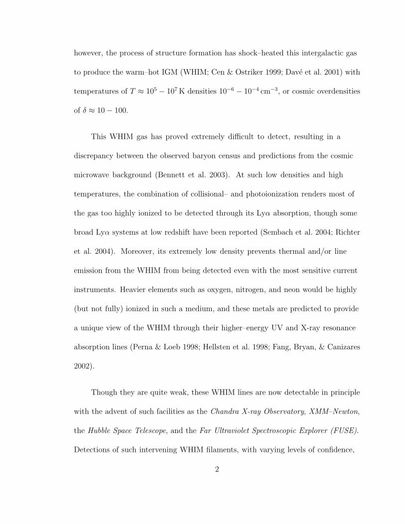
however, the process of structure formation has shock–heated this intergalactic gas

to produce the warm–hot IGM (WHIM; Cen & Ostriker 1999; Dave et al. 2001) with

temperatures of T ≈ 105 − 107 K densities 10−6 − 10−4 cm−3, or cosmic overdensities

of δ ≈ 10 − 100.

This WHIM gas has proved extremely difficult to detect, resulting in a

discrepancy between the observed baryon census and predictions from the cosmic

microwave background (Bennett et al. 2003). At such low densities and high

temperatures, the combination of collisional– and photoionization renders most of

the gas too highly ionized to be detected through its Lyα absorption, though some

broad Lyα systems at low redshift have been reported (Sembach et al. 2004; Richter

et al. 2004). Moreover, its extremely low density prevents thermal and/or line

emission from the WHIM from being detected even with the most sensitive current

instruments. Heavier elements such as oxygen, nitrogen, and neon would be highly

(but not fully) ionized in such a medium, and these metals are predicted to provide

a unique view of the WHIM through their higher–energy UV and X-ray resonance

absorption lines (Perna & Loeb 1998; Hellsten et al. 1998; Fang, Bryan, & Canizares

2002).

Though they are quite weak, these WHIM lines are now detectable in principle

with the advent of such facilities as the Chandra X-ray Observatory, XMM–Newton,

the Hubble Space Telescope, and the Far Ultraviolet Spectroscopic Explorer (FUSE).

Detections of such intervening WHIM filaments, with varying levels of confidence,

2

have been reported along several lines of sight (Nicastro et al. 2005a,b; Mathur et al.

2003; Fang et al. 2002). The total baryonic mass reported by Nicastro et al. (2005a)

is indeed consistent (within the admittedly large errors) with the aforementioned

baryon deficit at low redshifts.

Since most galaxies are expected to trace the same cosmic overdensities as the

web of WHIM filaments, it would be no surprise if the Galaxy itself resided in such

a filament. Indeed, X-ray spectra of several quasars have shown likely z = 0 Ovii

absorption, but it is unclear whether this absorption is actually due to the nearby

WHIM or is instead a component of the Galaxy itself, such as a hot halo or corona

(or some combination of the two). Some Ovii absorption has indeed been found

within 50 kpc of the Galaxy (Wang et al. 2005), but this is unlikely to be uniformly

distributed. Simulations of the Local Group strongly indicate that a large amount

of warm–hot gas is expected near zero redshift (Kravtsov et al. 2002). Thus, in

reality the X-ray absorption is likely to be caused by a combination of Galactic

and extragalactic components, perhaps with one dominating the other in certain

directions.

Further complicating the issue is the presence of other gaseous components

of unknown origin. H I high–velocity clouds (HVCs) have a velocity distribution

inconsistent with Galactic rotation and therefore are thought to be either neutral

gas high in the Galactic halo or cooling, infalling gas from the surrounding IGM.

Along many lines of sight studied with FUSE, high–velocity Ovi absorption lines at

3

velocities coincident with the H i HVCs are seen, while in some other directions the

high–velocity Ovi is present even in the absence of H i emission at that velocity

(Sembach et al. 2003). Some of these latter, unassociated Ovi HVCs were found to

be at rest in the Local Group rest frame (as a population), indicating that they may

be extragalactic in origin (Nicastro et al. 2003). On the other hand, many of these

Ovi HVCs also show absorption from lower ionization states that are unlikely to

arise in a low–density, warm–hot IGM (Sembach 2003).

While the evidence appears to point to both Galactic and extragalactic

characteristics for the Ovi HVCs, their connection to the highly–ionized gas seen

in X-rays (if any) is unknown. Part of the problem has been the tremendous

amount of Chandra observing time that is required to obtain a high–quality grating

spectrum of an extragalactic source: since X-ray telescopes are essentially photon

counting devices, thousands of scarce (compared to optical telescopes), high–energy

X-ray photons must be collected for each resolution element in order to detect even

relatively strong WHIM lines (∼ 20 mA, corresponding to NOVII ≈ 1016 cm−2). In

the past few years, however, there have been several opportunities to overcome this

difficulty: observing AGN only during extremely bright flares (as with Mrk 421),

re–analyzing long exposures that were originally performed for other purposes (Mrk

279), and co–adding many short calibration observations of the same object taken

over the past seven years (PKS 2155–304).

4

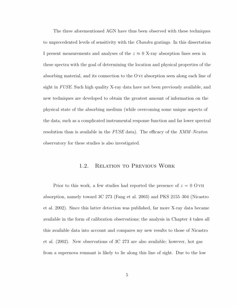
The three aforementioned AGN have thus been observed with these techniques

to unprecedented levels of sensitivity with the Chandra gratings. In this dissertation

I present measurements and analyses of the z ≈ 0 X-ray absorption lines seen in

these spectra with the goal of determining the location and physical properties of the

absorbing material, and its connection to the Ovi absorption seen along each line of

sight in FUSE. Such high quality X-ray data have not been previously available, and

new techniques are developed to obtain the greatest amount of information on the

physical state of the absorbing medium (while overcoming some unique aspects of

the data, such as a complicated instrumental response function and far lower spectral

resolution than is available in the FUSE data). The efficacy of the XMM–Newton

observatory for these studies is also investigated.

1.2. Relation to Previous Work

Prior to this work, a few studies had reported the presence of z = 0 Ovii

absorption, namely toward 3C 273 (Fang et al. 2003) and PKS 2155–304 (Nicastro

et al. 2002). Since this latter detection was published, far more X-ray data became

available in the form of calibration observations; the analysis in Chapter 4 takes all

this available data into account and compares my new results to those of Nicastro

et al. (2002). New observations of 3C 273 are also available; however, hot gas

from a supernova remnant is likely to lie along this line of sight. Due to the low

5

velocity resolution of Chandra (∼ 700 km s−1 at the Ovii wavelength), absorption

from the remnant would be fully blended with any WHIM or Galactic corona Ovii,

making this sightline of limited use. Constrained simulations of the Local Group by

Kravtsov et al. (2002) provide a strong theoretical basis for the existence of z = 0

WHIM while predicting roughly where the strongest absorption can be expected.

In fact, far more literature on the z > 0 WHIM has been published. Fang et al.

(2002), Mathur et al. (2003), and McKernan et al. (2003) reported early tentative

detections of the WHIM toward several sources, and I address the Fang et al. (2002)

detection of z = 0.055 Oviii toward PKS 2155–304 in Chapter 4. By far the most

confident detection of the z > 0 WHIM to date is in the Mrk 421 spectrum (which

I analyze in Chapter 2) by Nicastro et al. (2005a). Two WHIM filaments were

unambiguously detected in this spectrum, allowing the temperature density, and

relative metal abundances of the WHIM to be estimated. These provide a valuable

set of parameters to compare with those derived from the z = 0 absorption. The

detections of these WHIM filaments are also revisited with XMM–Newton in Chapter

5.

1.3. Scope of the Dissertation

The data, analysis, and interpretation of the X-ray and UV data along three

extragalactic sightlines are the focus of this dissertation. Owing to the individual

6

peculiarities of the observations and the variety of analysis techniques required

for the different data, the three following chapters are each devoted to one line of

sight: Markarian 421 (Chapter 2), Markarian 279 (Chapter 3), and PKS 2155–304

(Chapter 4). Chapter 5 presents a comparison of the XMM–Newton data of Mrk

421 with the previously reported Chandra detection of two WHIM filaments along

this line of sight, and quantitatively describes why XMM is unable to detect these

filaments. Finally, I summarize the results of this dissertation and comment on

present and future avenues for this research.

A major fraction of the research presented in this dissertation has been

published in the scientific literature. Chapter 2 is largely taken from Williams et

al. 2005, ApJ, 631, 856; chapter 3 has appeared as Williams et al. 2006, ApJ, 645,

179; and most of chapter 5 also appears in Williams et al. 2006, ApJ, 642, L95.

7

Chapter 2

The Markarian 421 Sightline

Through a program of observing nearby blazars in outburst phases, we have

obtained high–quality Chandra and FUSE spectra of Mkn 421, sufficient to study in

detail the local WHIM (and Galactic halo/thick disk) absorption. Here I report on

these observations, and the inferred properties of the local absorption.

2.1. Observations and Data Preparation

2.1.1. Chandra

A full description of the Chandra observations, data reduction, and continuum

fitting can be found in Nicastro et al. (2005a); a brief summary follows. Mkn 421

was observed during two exceptionally high outburst phases for 100 ks each as part

of our Chandra–AO4 observing program: one at f0.5−2keV = 1.2 × 10−9 erg s−1 cm−2

with the Low Energy Transmission Grating (LETG) combined with the Advanced

CCD Imaging Spectrometer–Spectroscopic (ACIS-S; Garmire et al. 2003) array,

and another at f0.5−2keV = 0.8 × 10−9 erg s−1 cm−2 with the High Resolution

8

Camera–Spectroscopic (HRC-S; Murray & Chappell 1985) array and LETG. Each

of these observations contains ∼ 2500 counts per resolution element at 21.6 A.

Additionally, another short observation of Mkn 421 was taken with HRC/LETG

(29 May 2004), providing another 170 counts per resolution element. These three

spectra were combined over the 10–60 A range to improve the signal–to–noise ratio

(S/N≈ 55 at 21 A with 0.0125 A binning). The final coadded spectrum of Mkn 421

is one of the best ever taken with Chandra: it contains over 106 total counts with

∼ 6000 counts per resolution element at 21.6 A, providing a 3σ detection threshold

of Wλ ≈ 2 mA (NOVII = 8 × 1014cm−2 for an unsaturated line).

Effective area files (ARFs) for each observation were built using CIAO1 v3.0.2

and CALDB2 v2.2.6. Those pertaining to the ACIS/LETG observations were

corrected for the ACIS quantum efficiency degradation3 (Marshall et al. 2003). For

the HRC/LETG observations, the standard ARFs were used. Each ARF was then

convolved with the relevant standard redistribution matrix file (RMF), and the

convolved RMFs were weighted by exposure time, rebinned to the same energy scale,

and averaged to provide a response file for the coadded spectrum.

Using the CIAO fitting package Sherpa4, we initially modeled the continuum

of Mkn 421 as a simple power law and a Galactic absorbing column density of

1cxc.harvard.edu/ciao/

2cxc.harvard.edu/caldb/

3See also cxc.harvard.edu/ciao/why/acisqedeg.html

4cxc.harvard.edu/sherpa/

9

NH = 1.4 × 1020 cm−2 (Dickey & Lockman 1990), excluding the 48–57 A HRC chip

gap region. Metal abundances for the Galactic gas were then artificially adjusted to

provide a better fit around the O I and C I K–edges near 23 A and 43 A respectively.

This is not intended to represent actual changes to the absorber composition, but

rather to correct uncertainties in the instrument calibration. These adjustments

affect the continuum mostly near the carbon, oxygen, and neon edges, but individual

narrow absorption lines are unaffected. After this fit there were still some systematic

uncertainties in the best–fit continuum model; these were corrected with broad

(FWHM = 0.15 − 5 A) Gaussian emission and absorption components until the

modeled continuum appeared to match the data upon inspection. Indeed, the

residuals of the spectrum to the final continuum model have a nearly Gaussian

distribution, with a negative tail indicating the presence of narrow absorption lines

(see Nicastro et al. 2005a, Figure 8).

2.1.2. FUSE

Mkn 421 was also observed with FUSE as part of our Director’s Discretionary

Time observing program on 19–21 January 2003 for a total of 62.8 ks. An additional

21.8 ks observation from 1 December 2000 was also available in the archive. We used

the time–tagged, calibrated data from only the LiF1A detector, since inclusion of

the LiF2B data provides a small (∼ 20%) increase in S/N but degrades the overall

10

spectral resolution.5 These two observing programs consist of four observations,

which in turn contain a total of 29 individual exposures. The wavelength scales of

each observation’s constituent exposures were cross–correlated and shifted (typically

by 1–2 pixels) to account for slight uncertainties in the wavelength calibration. The

exposures for each observation were checked for consistency and coadded, weighted

by exposure time. The resulting four spectra were then cross-correlated against

each other, coadded (with a ∼ 10% downward shift in flux applied to the 2000

observation due to source variability), and binned by 5 pixels (0.034 A, or one–half

of the nominal 20km s−1 resolution) providing a S/N of 17 near 1032 A.

To check the absolute wavelength calibration we followed the method of Wakker

et al. (2003), using their 4–component fit to the Murphy et al. (1996) Green Bank

H I–21 cm data as a velocity reference. They find four main components of H I

emission with an NH–weighted average velocity of −31.7km s−1. In the FUSE

spectrum, the Si II λ1020.699 A and Ar I λ1048.220 A lines are expected to trace the

same gas as the H I emission. Each UV line was fit with two Gaussian components

in Sherpa, giving average velocity offsets of −30.9 and −34.9km s−1 respectively.

These agree well with the H I data, though the slight difference between the Ar I and

Si II measurements suggest at least a ∼ 4km s−1 intrinsic wavelength uncertainty.

5See the FUSE Data Analysis Cookbook v1.0, fuse.pha.jhu.edu/analysis/analysis.html

11

2.2. Line Measurements

To find and identify narrow absorption lines in the Chandra spectrum of

Mkn 421, we visually inspected small (2–5 A) regions of the spectrum, beginning

around the rest wavelength of OviiKα (21.602 A) since this tends to be the strongest

z = 0 X-ray absorption line (e.g. Nicastro et al. 2002; Fang et al. 2003; Chen et al.

2003). Three OviiKα (Figure 2.1) absorption features were found: one at z = 0,

one at z = 0.011, and one at z = 0.027 (with typical redshift errors of 0.001).

There is also a strong feature which is ∼ 3σ from the OvKα rest wavelength, but is

more likely OviiKα at v ≈ +900km s−1 relative to the blazar. A close pair of lines

consistent with Lyα at this velocity has been observed (Shull et al. 1996; Penton et

al. 2000), so this may be indicative of an inflow to Mkn 421 or uncertainty in the

blazar redshift (based on rather old spectrophotometric measurements by Margon

et al. 1978). A weak OviKα line is seen at the rest wavelength of 22.02 A. Other

regions of the spectrum were then searched for lines corresponding to these systems,

with particular emphasis paid to strong transitions of the most abundant elements

(C, N, O, and Ne). All in all there were 13 lines marginally or strongly detected

at z ≈ 0 (including the Nvii, Ov, and Arxv upper limits), 3 at z = 0.011, and 7

at z = 0.027. The latter two systems are the subject of other papers (Nicastro et

al. 2004a,b) and thus will not be discussed further here.

12

These 13 z = 0 X-ray lines were fitted in Sherpa with narrow Gaussian features

superposed on the fitted continuum described in §2.1.1 (see Figure 2.1). We are

excluding the strong O I (23.51 A) line since it arises in the neutral ISM and is

not of interest here, as well as the O2 (23.34 A) absorption since it coincides with

a strong instrumental feature and cannot be accurately measured. Due to the

FWHM = 0.04 A (∼ 600km s−1) LETG resolution the lines are all unresolved,

so only the position and equivalent width of each line are measured. Errors are

calculated using the “projection” command in Sherpa, allowing the overall continuum

normalization to vary along with all parameters for each line. The resulting line

parameter estimates are presented in Table 2.1. The ∼ 0.02 A systematic wavelength

uncertainty of the LETG6 is in most cases larger than the statistical uncertainty

of the line centroid; thus, Table 2.1 lists whichever is greater. Additionally, a

meaningful upper error bar on the Cvi equivalent width could not be calculated

with Sherpa. In this case, the FWHM was frozen at the instrumental resolution and

the error was recalculated; a visual inspection confirms the new limit to be more

reasonable. Upper limits for the Ov, Nvii, Arxv, and Nex lines were calculated

with both the position and FWHM frozen.

The FUSE spectrum (Figure 2.2) shows a strong, broad low–velocity Ovi

1032 A absorption line at z ≈ 0 due to gas in the Galactic thick disk and halo

(Savage et al. 2003). An asymmetric wing on the red side of this line is evident,

6cxc.harvard.edu/cal/

13

possibly a kinematically distinct HVC. We fitted the Ovi 1032 A line in Sherpa

using a constant local continuum (in a ±2 A window) and two Gaussian absorption

components: one for the v ≈ 0 OviLV line, and one at v ≈ 100km s−1 for the

HVC. No H2 contamination is seen at the Ovi 1032 A wavelength when absorption

templates are fit to the other H2 lines seen in the spectrum. The 1037 A line is

somewhat blended with a single H2 absorption line; this is taken into account with

another narrow Gaussian. From this fit, we find equivalent widths of 18.6 ± 5.6 mA

for the 1032 A HVC and 270.7 ± 7.9 mA for the Galactic component. The best–fit

model for the HVC is fairly robust and not sensitive to variations in the initial

parameters; however, the derived equivalent width of 18.5 ± 5.6 mA is lower than

the 37 ± 11 ± 29 mA (errors are statistical and systematic, respectively) measured

by Wakker et al. (2003) in the initial 21.8 ks observation. They employed a direct

integration method which may not have taken into account the substantial blending

of the Galactic OviLV with the HVC. Our total Ovi equivalent width (LV+HVC

= 279 ± 10 mA) is in good agreement with their value of 285 ± 20 mA.

Deblending the Ovi 1037 A line is less certain due to the presence of adjacent

Galactic C II and H2 absorption. A flat continuum was again employed from

1035 − 1040 A and single Gaussian components were used to fit the C II, Ovi,

and H2 absorption lines. The HVC on the 1032 A Ovi line should also appear at

∼ 1038 A with Wλ = 0.50×Wλ(1032 A). Although this component is too weak to be

detected directly, it could cause the measurement of the Galactic LV–Ovi 1037 A

14

line to be systematically high. Another absorption Gaussian with one–half of the

1032 A HVC equivalent width (and with the same FWHM and velocity offset) was

included in the 1037 A Ovi line fit to account for this. Table 2.1 lists the measured

properties of the OviLV and HVC absorption lines.

2.3. Absorption Line Diagnostics

2.3.1. Doppler Parameters

To convert the measured equivalent widths to ionic column densities, we

calculated curves of growth for each absorption line over a grid of Doppler

parameters (b = 10− 100km s−1) and column densities (log NH/cm−2 = 12.0− 18.0),

assuming a Voigt line profile. Since the X-ray lines are unresolved, b cannot be

measured directly. It can, however, be inferred from the relative strengths of the three

measured Ovii K–series lines. These lines are produced by the same ionic species,

so in an unsaturated medium Wλ ∝ fluλ2 where flu is the oscillator strength. The

expected equivalent width ratio of Ovii Kβ to Kα is then Wλ(Kβ)/Wλ(Kα) = 0.156,

so the measured value of 0.49 ± 0.09 indicates that the Kα line is saturated. On the

other hand, the measured Ovii Kγ/Kβ ratio is 0.43 ± 0.16, in agreement with the

predicted (unsaturated) value of 0.34.

15

These line ratios by themselves are insufficient to determine the physical state

of the Ovii–absorbing medium since b and NOVII are degenerate: the Kα line

saturation could be due to high column density, low b, or a combination of both.

However, given an absorption line with a measured equivalent width and known

fluλ2 value, the inferred column density as a function of the Doppler parameter can

be calculated. The measured equivalent width (and errors) for each transition thus

defines a region in the NOVII − b plane. Since the actual value of NOVII is fixed, b and

NOVII can be determined by the region over which the contours “overlap;” i.e. the

range of Doppler parameters for which the different transitions provide consistent

NOVII measurements.

Figure 2.3 shows such 1σ contours for the three measured Ovii transitions.

As expected, the inferred NOVII is nearly constant in the unsaturated regime (large

b), and rises sharply at low b as the lines begin to saturate. At each value of b, the

differences ∆(log Nαβ) = log(NKα)−log(NKβ) and ∆(log Nαγ) = log(NKα)−log(NKγ)

were calculated, along with the errors on each ∆(log N). The quantity ∆(log Nαβ)

is consistent with zero at the 1σ and 2σ levels for 15 < b < 46km s−1

and 13 < b < 55km s−1 respectively, while ∆(log Nαγ) provides limits of

31 < b < 50km s−1 and 24 < b < 76km s−1 respectively. Since ∆(log Nαγ) provides a

more stringent lower limit on b while ∆(log Nαβ) better constrains the upper limit, we

thus assume a 1σ range of 31 < b < 46km s−1, and a 2σ range of 24 < b < 55km s−1.

It should be noted that Figure 2.3 also shows some overlap between the Kα and Kγ

16

at b ∼< 12km s−1; however, this solution is unlikely given the lower limit provided by

the Kβ line. Moreover, b = 12km s−1 implies a maximum temperature (assuming

purely thermal motion) of Tmax = 1.3 × 105 K; such a low temperature is unlikely to

produce the observed strong high–ionization lines.

A similar analysis is not as effective when applied to the strong OviLV UV

doublet (from the thick disk), since these lines are only slightly saturated: the

measured Wλ ratio is 0.61 ± 0.04, compared to the expected unsaturated value of

0.50. When the inferred NOVI is calculated as a function of b for both lines of the

OviLV doublet, the predicted NOVI values are consistent over b = 34 − 112km s−1

(at the 2σ level; see Figure 2.4). Since the OviLV 1032 A line is fully resolved by

FUSE (∼ 15 resolution elements across the line profile) and relatively unblended,

its Doppler parameter can be estimated much more accurately using the measured

line width and strength. In an unsaturated absorption line, FWHM = 2(ln 2)1/2b;

however, the measured FWHM increases if the line is saturated. We compensated for

this by calculating Voigt profile FWHMs on a grid of NOVI and b, and determining

the region consistent with the OviLV 1032 A FWHM measurement of 152± 7km s−1

(or b = 91 ± 4km s−1 assuming no saturation).

When the FWHM–derived contour is overlaid on the NOVI − b contour

inferred from the equivalent width measurement of the LV–Ovi 1032 A line, the

two regions overlap nearly orthogonally (Figure 2.4) leading to a constraint of

b(OviLV)= 80.6± 4.2km s−1. This is ∼ 2σ lower than the unsaturated FWHM, once

17

again confirming that the OviLV is only weakly saturated. At this b the inferred

column densities from the two lines of the OviLV doublet differ by 1.3σ but this is

only a minor discrepancy and likely due to errors introduced by the blending of the

1037 A line; thus, we will only consider results from the more reliable 1032 A line

measurement. However, at no value of the Doppler parameter do the 1032 A, 1037 A,

and OviKα lines all produce a consistent NOVI measurement; in fact, the OviKα

column density is a factor of ∼ 4 higher than that inferred from the UV data. This

discrepancy is discussed further in §2.4.1.

2.3.2. Column Densities

The Doppler parameters measured for the Ovii (31km s−1 < b < 46km s−1)

and OviLV (b = 80.6 ± 4.2km s−1) absorption are inconsistent at the ∼ 3σ level,

indicating the presence of at least two distinct components: the Galactic thick–disk

gas traced by broad v ≈ 0 OviLV absorption, and another lower–b phase, possibly

of extragalactic origin, traced by the Ovii absorption lines. It cannot be assumed

a priori that any given line (other than those used to determine b) originates in

one phase or another; moreover, the uncertainty in the calculated column density

depends not only on the equivalent width error but also the error in b. To take

this into account, for each ion the derived column density log Ni and its ±1σ limits

were averaged over the ±1σ ranges of both measured Doppler parameters. As it

turns out, the choice of b does not make a significant difference since all other

18

lines (besides the Ovii and OviLV absorption) are essentially unsaturated; i.e., the

difference in Ni calculated with the OviLV and Ovii Doppler parameters is small

compared to the 1σ error on the equivalent width measurements. Even so, to avoid

possible systematic errors, we assumed b = 80.6 ± 4.2km s−1 for those lines likely to

originate in the Galactic thick disk (OviLV, Ov, and Cv), and b = 31 − 46km s−1

for all other species. The derived ionic column densities are listed in Table 2.1

2.3.3. Temperature and Density Constraints

At densities such as those found in the Galactic interstellar medium (ISM;

ne ≈ 1 cm−3), photoionization is unimportant because thermal collisions are by far

the dominant ionization source. This is also the case for very high temperatures

(T ∼> 107 K) even at low densities, since the collisional rate is greater than

the photoionization rate. However, at the low densities typically found in the

intergalactic medium (ne = 10−6 − 10−4 cm−3), photoionization from the diffuse

UV/X-ray background begins to play a greater role by enriching the abundances of

highly–ionized elements at typical WHIM temperatures (log T (K) ≈ 5 − 7) relative

to those expected from pure collisional ionization (Nicastro et al. 2002; Mathur et al.

2003). It is thus imperative that the ionizing background be taken into account in

order to accurately predict ionic abundances in the WHIM.

19

Version 90.04 of the ionization balance code Cloudy (Ferland 1996) was used to

compute collisional– plus photoionization hybrid models for the absorbing medium.

Relative ionic abundances were computed over a grid of log T (K) = 4.5 − 7.4 and

log ne(cm−3) = −7−0, with a step size of 0.1 dex in both log ne and log T . Initially, a

rigid scaling of [Z/H] = −1 for all metals was assumed. For the ionizing background

we employed the Sternberg et al. (2002) fit to the metagalactic radiation field:

Jν =

Jν0

(

νν0

)

−3.131 < ν

ν0

< 4

2.512 × 10−2Jν0

(

νν0

)

−0.46νν0

> 4

(2.1)

where here Jν0 = 2×10−23 ergs s−1 cm−2 Hz−1 sr−1 and ν0 = 13.6 eV. The total flux of

ionizing photons is then given by fγ = 4π∫

∞

ν0(Jν/hν)dν = 1.3×104 photons s−1 cm−2,

and the ionization parameter is log U = log(fγ/c) − log ne = −6.36 − log(ne) where

ne is the electron density in cm−3.

Using the ionic abundances calculated with Cloudy, we derived expected

abundance ratios for all observed ions at each point in the log ne − log T plane.

Since any given density and temperature uniquely determines a set of abundance

ratios (Na/Nb for all ions a and b), the problem can be inverted: any value of Na/Nb

defines a curve in the log ne − log T plane, i.e. a set of temperatures and densities

which can produce the measured ratio. When the errors on Na/Nb are taken into

account, the curves become contours, and the overlap between two or more contours

defines the temperatures and densities for which the measured ratios are consistent.

20

This is analogous to the method used in §2.3.1 to determine Doppler parameters for

OviLV and Ovii.

The most powerful diagnostics are those using ratios between different ions of

the same element, since these ratios are independent of the relative metal abundances.

Unfortunately the Nvii/Nvi and Nex/Ne ix upper limits are not stringent enough

to place meaningful constraints on the temperature and density. Figure 2.5 shows

the log ne − log T contours for ratios between the X-ray OviKα, Ovii, and Oviii

lines as well as the OviHVC/Ovii ratio. The X-ray line ratios are inconsistent with a

high–density (ne ∼> 10−3cm−3), high–temperature (log T > 6.2) medium, and instead

converge on a partially photoionized plasma with ne = 10−4.7 − 10−3.9 cm−3 (from

the overlap between the OviKα/Ovii and Oviii/Ovii contours) and T = 105.5−5.7 K

(from the limits provided by OviKα/Ovii in this density range). These ranges of

temperatures and densities are in line with those expected from WHIM gas (Dave et

al. 2001). Of course, this is all contingent on the OviKα line being a reliable tracer

of NOVI; this caveat is discussed in detail in §2.4.

On the other hand, the OviHVC/Ovii ratio overpredicts the temperature by

at least an order of magnitude for all values of log ne—in order to be consistent

with the Oviii/Ovii ratio, the OviHVC/Ovii ratio would need to be stronger by a

factor of ∼ 2.5 (or ∼ 3.5σ). It is possible that the HVC is not a physically distinct

component, but is instead the result of some systematic error (such as fixed pattern

noise or an unexpected anomaly in the Galactic OviLV velocity distribution). In this

21

case, the Ovi associated with the Ovii and Oviii may be completely blended with

the thick–disk OviLV and thus unmeasurable. Consistency with the Oviii/Ovii

ratio (in the collisional ionization regime) requires log(NOVI/NOVII) ≈ −2.5, or

roughly 20% of the Galactic UV Ovi absorption. Although it appears that the Ovi

HVC as measured cannot originate in the same medium as the Ovii absorption, we

suspect that additional atomic physics may be at work here and could in principle

reconcile this disagreement (see §2.4.1).

While the OviKα/Ovii and Oviii/Ovii ratios provide strong constraints,

it is important to consider other ion ratios as well (particularly since the OviKα

and 1032 A Ovi column densities disagree). Figure 2.6 shows the log ne − log T

contours for several different ion ratios, all calculated relative to Ovii since the error

on NOVII is small. With a rigid metallicity shift relative to solar, the Ne ix/Ovii

Oviii/Ovii, and OviKα/Ovii ratios are not all consistent with each other for

any combination of temperature and density; however, the consistency can be

improved with adjustments to the [Ne/O] ratio (see §2.4.1). Both the Cvi/Ovii

and Nvii/Ovii measurements are consistent with a high– or low–density medium

at solar abundances.

Limits on the temperature of the Galactic thick–disk absorption can be derived

in a similar fashion, although it is not the primary focus of this work and there are

far fewer measured lines to work with. The most accurately–measured line is the

OviLV; additionally, Cv and Nvi X-ray lines are measured, and upper limits have

22

been determined for Ov and Nvii. Figure 2.8 shows the temperature constraints

derived for this Galactic absorption, assuming pure collisional ionization. The

Ov/OviLV and Nvii/Nvi upper limits provide metallicity–independent constraints

of log T > 5.39 and log T < 6.64 respectively. A more stringent upper limit on

temperature of log T < 6.03 is provided by the Nvii/OviLV ratio, but this is

somewhat dependent on [N/O]. Within this range the Cv/OviLV ratio provides an

even stricter limit of 5.3 < log T < 5.7, but again this depends on [C/O]. At these

temperatures the expected Ovii column density is at most an order of magnitude

less than measured; thus, the OviLV, Ovii, and Oviii cannot all originate in the

same phase assuming pure collisional ionization (see also Mathur et al. 2003).

2.4. Discussion

Our Chandra and FUSE observations have provided a wealth of data on

absorption near the Galaxy, constraining the temperature and density tightly

(log T (K) = 5.5 − 5.7 and ne = 10−4.7 − 10−3.9 cm−3 when the OviKα measurement

is included), which are conditions suggestive of the local group intergalactic medium

and require supersolar [Ne/O]. Here we first examine the assumptions that have led

us to these results (§2.4.1), and then we discuss their implications for the location of

the absorbing gas (§2.4.2), subject to these caveats.

23

2.4.1. Potential Caveats

The Ovi Discrepancy

The interpretation of the UV and X-ray data are particularly important, since

(as Figure 2.5 shows) the combined Oviii/Ovii and Ovi/Ovii ratios can provide

tight constraints on the absorber temperature and density simultaneously (see also

Figure 5 in Mathur et al. 2003). However, in this case the Ovi column density

inferred from the OviKα is a factor of ∼ 4 higher than the combined 1032 A low– and

high–velocity components. Since both the X-ray and UV transitions trace the same

atomic state, the inferred column densities should match. A similar disagreement

has been seen in intrinsic AGN absorption systems (see Krongold et al. 2003;

Arav et al. 2003); however, in these cases it is typically attributed to saturation

or a velocity–dependent covering factor, neither of which is relevant to this z ≈ 0

absorption.

On the other hand, our OviKα measurement provides a test for these

attributions; the local absorption, after all, is likely a dramatically different

physical system than an AGN outflow, yet the same conflict arises. A macroscopic

explanation does not adequately describe how this discrepancy is seen in both

physical systems, so the actual reason may lie in the atomic physics of highly ionized

plasmas. For example, some fraction of the Ovi may be excited through collisions or

recombination from Ovii, and thus unable to produce 1032 A absorption while still

24

absorbing OviKα photons. While a scenario that produces significant depopulation

of the Ovi ground state is difficult to envisage in such a low density plasma, we

are investigating further the statistical equilibrium of Ovi including photoexcitation

and recombination in order to study such effects in more detail. However, it

should be emphasized that this is not an isolated case so there must be a physical

explanation for the Ovi discrepancy, and the resolution of this paradox is crucial to

our understanding of Ovi UV and X-ray absorption and how it relates to the Ovii.

There is also the possibility that the line was misidentified as OviKα, and

is actually another intervening Ovii absorption line at z = 0.0195. This latter

explanation is unlikely since no other absorption lines at this redshift are seen in the

FUSE or Chandra spectra; additionally, this would require the line to fall exactly

on the Ovi rest wavelength, which seems like an improbable coincidence. Another

possibility is that the theoretical oscillator strength of the OviKα transition is

incorrect, but the value given in Pradhan (2000) would need to be low by a factor

of ∼ 2 − 4, in sharp contrast to the successful calculations of flu for inner shell

transitions in other ions in the same paper. Nevertheless, due to the discrepancy

between the UV and X-ray Ovi column density measurements, we present both

possibilities: either (a) the OviKα line measures NOVI, or (b) it does not and is thus

ignored.

25

Absorption Components

The Doppler parameter measurements indicate the existence of two distinct

components along the Mkn 421 line of sight: one seen in the thick–disk OviLV

1032 A absorption with bLV = 80.6 ± 4.2km s−1, and the Ovii absorber with

bOVII = 31 − 46km s−1 (1σ limits). The Ovi HVC may represent a third phase (if

case (b) above is correct) with bHVC = 35+18−10km s−1 (from the FWHM measurement).

This agrees surprisingly well with the Ovii b measurement, and is consistent with

numerical simulations of the nearby IGM (Kravtsov et al. 2002). However, the

extremely low OviHVC/Ovii ratio requires a temperature much higher than the

upper limit provided by bOVII. In order for the HVC to trace the same gas as

Ovii (case a), then, the aforementioned atomic physics effects would need to be

suppressing Ovi HVC absorption and not the OviLV line. Sembach et al. (2003) list

mean Doppler parameters for a variety of HVCs, both Galactic and probable Local

Group; unfortunately, the dispersion in these values and the errors on bOVII and bHVC

measured here are both too large to associate the components presented here to one

of their classifications.

It is also important to note that our analysis assumes a single phase origin

for the included X-ray lines. This assumption is consistent with the data, given

the good agreement between the three Ovii lines in the calculated ranges of b and

NOVI (Figure 2.3). Even so, if any of the ionic species arises in more than one

26

phase along the line of sight, our results could be affected. For example, a Galactic,

purely collisionally ionized medium can in principle reproduce the observed relative

abundances of Oviii, Ovii, OviKα, and Ne ix if several unresolved components

are invoked to explain this absorption. However, the simplest explanation (a

single–phase, low–density, partially photoionized extragalactic absorber) is fully

consistent with all of these line measurements, and the similarity of the derived

absorber properties to expectations for the local WHIM lend further support to this

model (see §2.4.2).

Abundances

Due to the uncertainty associated with the OviKα absorption, metal abundances

relative to oxygen play a particularly important role in this analysis. By adjusting

the metal abundances of the absorbing gas, the consistency of the solutions can in

principle be improved with and without the OviKα measurement. Although the

log ne− log T contour plots are useful for finding solutions, they cannot easily be used

to determine the effects of changes in elemental abundances; thus, Figure 2.9 shows

Ni/NOVII as a function of log T for log ne = −3.9 and Figure 2.10 for log ne = 0. In

these figures, the y–ranges given by the measured ratios (thick lines) shift up and

down as a result of decreases and increases in the abundances relative to oxygen,

respectively; thus different parts of the theoretical curves would be in bold, moving

the allowed temperature ranges (shown in the lower panel) to the left or right. Solar

27

abundances here are taken to be the Cloudy 90 defaults (Ferland 1996; Grevasse &

Anders 1989).

In case (a), i.e. if the OviKα measurement of NOVI is correct, then the

temperature and density of the absorber are tightly constrained in a metallicity–

independent manner, and relative abundances for other elements can be estimated.

Under this assumption, the oxygen ion ratios are consistent within a range

of ne = 10−4.7 − 10−3.9 cm−3; however at solar abundances the Ne ix/Ovii

ratio demands higher temperatures than allowed by the OviKα/Ovii ratio.

Over this range of densities, the permitted abundances of neon, carbon, and

nitrogen abundances relative to oxygen (that is, the range of abundances which

produce line ratios consistent with both OviKα/Ovii and Oviii/Ovii) are then

0.6 ≤[Ne/O]≤ 2.2, −0.8 ≤ [C/O]≤ 0.3, and [N/O]≤ 0.9. Note that supersolar

[Ne/O] has also been observed in the z = 0 absorber toward PKS2155–304 (Nicastro

et al. 2002). The improvement in the fit from supersolar [Ne/O] is shown in Fig 2.7.

Note, however, that in this case the discrepancy between the OviKα and 1032 A

measurements becomes even more severe. Since the bulk of the OviLV cannot be

associated with the Ovii due to the different Doppler parameters, the UV Ovi

component associated with the WHIM (hence the OviKα) must be substantially

weaker than the Galactic Ovi absorption; thus the discrepancy is correspondingly

larger.

28

On the other hand, if (b) the OviKα line is ignored then the relative abundances

in the absorber can be adjusted such that the measured line ratios are consistent

with either a low– or high–density absorber. As shown in Figure 2.6, a high–density,

collisionally–ionized medium fits the data with solar abundances. Assuming this is

the case, the temperature is then completely constrained by the Oviii/Ovii ratio

at log T = 106.1−6.2 K, and the relative abundances consistent with the Oviii/Ovii

ratio in this temperature range are −0.6 ≤[Ne/O]≤ 0.6, −0.6 ≤[C/O]≤ 0.3, and

[N/O]≤ 0.4.

The requirement that [Ne/O] be supersolar does not affect the viability of the

partially–photoionized model: in both the ISM and low–z IGM, [Ne/O] is observed

to be significantly larger than the solar value (e.g. Paerels et al. 2001; Nicastro

et al. 2005a). This may be an intrinsic property of the enriched gas ejected into

the IGM and ISM, or instead could be due to depletion of C, N, and O onto dust

grains in supernova ejecta or quasar winds (Whittet 1992; Elvis et al. 2002). If the

dust destruction timescale is long and the IGM is continuously enriched by this

latter mechanism, then the observed supersolar [Ne/O] would be expected. All of

these enrichment scenarios are quite uncertain, but few (if any) are able to produce

[Ne/O]< 0. Indeed, the solar neon abundance itself is quite uncertain since it is

inferred from solar wind measurements. The increase in the solar neon abundance

proposed by Drake & Testa (2005) is supported by these observations, and may

provide another physical argument for the lack of subsolar [Ne/O].

29

2.4.2. Where does the X-ray absorption originate?

Assuming the Ovii absorption system is homogeneous, its radial extent can be

estimated by calculating r ≈ NH/(µne), where µ ≈ 0.8, log(nO/nH) = −3.13 (solar

abundance), and

NH = NOVII ×(

NO,tot

NOVII

)

× 103.13−[O/H]. (2.2)

The second term in the equation is approximately unity, since over the range

of temperatures and densities implied from the Oviii/Ovii ratio, Ovii

is the dominant ionization state by at least an order of magnitude; thus,

log NH = log NOVII + 3.13 − [O/H] = {20.37 − ([O/H] + 1)} ± 0.11. The

measurement error on NOVII is small compared to the uncertainty range in ne,

so it can be disregarded. Assuming that (a) the OviKα line does measure NOVI,

the 2σ range of densities is −4.7 ≤ log ne ≤ −3.9, resulting in a radial extent of

r = (0.8 − 4.9) × 10−([O/H]+1) Mpc. These radial extents are consistent with those

expected from a Local Group medium or local filament interpretation for this

absorption (Nicastro et al. 2002, 2003) and too large to be confined within a Galactic

halo. The absorber extent could be marginally consistent with a Galactic corona if

the metallicity is high (r = 80 − 490 kpc, 2σ limits at solar metallicity); however,

such a scenario seems implausible, particularly if this corona primarily consists of

gas accreted from the metal–poor IGM.

30

It is unlikely that this absorption system, if extragalactic, is spherically

symmetric (particularly in a “local filament” interpretation). The total

mass in the Ovii system can be written as Mtot = f × (4/3)πr3(1.4nHmH),

where f (< 1) parameterizes the departure from spherical symmetry and

1.4nHmH ≈ nHmH + nHemHe. Replacing r with NH/(µne) and plugging in relevant

values,

Mtot = 9.9 × 1012M⊙(

10−3([O/H]+1))

(

ne

10−4 cm−3

)

−2

f (2.3)

This is several times larger than estimates of the total Local Group binding mass,

e.g. Mtot = (2.3± 0.6)× 1012M⊙ as calculated by Courteau & van den Bergh (1999).

Baryonic matter should only contribute ∼ 15% of this mass (if the baryon–to–dark

matter ratio is equal to the cosmological value), so our estimate appears high. This

discrepancy can be easily resolved with different values of [O/H] and f . For instance,

if we assume an oxygen abundance of 0.3 times solar rather than 0.1, then the range

of possible masses becomes 2.0 × 1011fM⊙ ≤ Mtot ≤ 7.9 × 1012fM⊙. Thus, unless

[O/H] is very high or f ≪ 1, the Ovii absorber almost certainly accounts for a

major fraction of the baryonic matter in the Local Group. This sightline may also

be probing gas that is not gravitationally bound to the Local Group (i.e., the Local

Filament), which may explain why our range of Mtot extends to such high values.

Although Collins et al. (2005) argue that a Local Group origin requires that the

31

Ovii absorbers contain too much mass, we see here that the total mass is in fact

consistent with expectations.

If this absorption does only trace the Local Group medium, then

constraints on the extent of the absorber can be derived by assuming

Mtot = 0.15MLG ≈ 3.5×1011M⊙. In this case, r3f = 3Mtot/(4π×1.4µnemH). Taking

the 2σ upper limit of log nH = −3.9, the 2σ lower limit on MLG = 1.1 × 1012M⊙,

and assuming f = 1, we obtain a lower limit of r > 0.2 Mpc for the Ovii absorption.

Similarly, the upper limit on the radius is r < 0.6f−1/3 Mpc. This seems somewhat

small compared to the actual size of the Local Group, but once again is dependent

on the geometry of the absorber. A value of f ≈ 0.1 brings this upper limit more in

line with the Mpc scales expected in the Local Group; this may indicate that the

Mkn 421 line of sight probes an extended, filamentary WHIM distribution. This

calculation also assumes that the density of the Local Group medium is constant

with radius, when the actual density profile is more likely centrally concentrated.

These measurements are also affected by the Ovi discrepancy: in case (b), only the

lower density limit of log(ne) > −4.7 (from the 2σ Ovi Kα upper limit) applies, so

the upper radius and mass limits are still valid. Nevertheless, the consistency with

the expected Local Group parameters is intriguing.

32

2.4.3. Comparisons to Other Studies

Kravtsov et al. (2002) used constrained simulations to study the properties

of the Local Supercluster region; sky maps produced from this simulation (their

Figure 5) show filamentary structures near the Mkn 421 direction, possibly

corresponding to the observed absorption. Additionally, they note that a Local

Group medium would exhibit a low Doppler parameter (b ∼< 60 km s−1) out to

distances of ∼ 7 Mpc, consistent with our Ovii measurement.

The inferred properties of the X-ray absorption along this line of sight also

appear similar to other observations: toward 3C 273, for example, Fang et al. (2003)

find 5.36 < log T < 6.08 and comparable Ovii column density; however, their

inferred Ovii Doppler parameter is significantly higher than that toward Mkn 421:

b > 100km s−1. On the other hand, the z = 0 absorber toward PKS 2155 − 304

(Nicastro et al. 2002) exhibits a temperature consistent with the Mkn 421 absorber,

yet inferred density about an order of magnitude lower. Compared to the two

intervening filaments seen toward Mkn 421 (Nicastro et al. 2005a), the density of

the z = 0 absorption agrees with the derived lower limits (log ne ∼> −5 for both

filaments), but the filaments appear to exhibit higher temperatures than that

derived for the local absorption. These variations along different lines of sight

simply demonstrate the complex nature of the absorption, and the diversity of

33

temperature and density environments produced in the structure formation process

(e.g., Kravtsov et al. 2002).

The detection of X-ray absorption lines toward the Large Magellanic Cloud

binary LMC X-3 by Wang et al. (2005) presents an important consideration for these

results as well. The measured Ovii and Ne ix equivalent widths and upper limits on

Oviii and OviiKβ are all consistent with the same lines measured toward Mkn 421

(albeit with much larger statistical errors). Although this detection provides evidence

of a hot intervening absorber between the Galaxy and LMC, it certainly does not

rule out a primarily extragalactic origin for the Mkn 421 absorber. Any absorption,

either Galactic or extragalactic, is likely to be inhomogeneous; thus, it’s entirely

plausible that the LMC X-3 sightline probes hot Galactic gas (perhaps enhanced by

winds or outflows from both the Galaxy and LMC), while the absorption toward

Mkn 421 is primarily due to low–density nearby WHIM gas.

2.5. Summary and Future Work

Through long–duration Chandra and FUSE observations of Mkn 421 in

outburst, we have obtained unprecedented measurements of a variety of z ≈ 0

absorption lines, many of which likely arise in extragalactic, partially photoionized

gas. A brief summary of our results follows.

34

1. The relative strengths of the three Ovii K-series lines imply 2σ Doppler

parameter constraints of 24 < b < 55 km s−1. This is inconsistent with the

value of b = 80.6 ± 4.2 km s−1 derived for the Galactic low–velocity Ovi,

indicating that the OviLV and Ovii likely arise in different phases. The Ovii

b value is, however, consistent with the local IGM simulations of Kravtsov et

al. (2002) out to distances of several Mpc.

2. A weak high–velocity Ovi 1032 A component also appears in the FUSE

spectrum. Although its width is consistent with the Ovii b measurement, the

OviHVC column density is too low to be associated with the Ovii absorption

unless T ∼> 107 K (which itself is ruled out by the upper limit on b). The

OviHVC may thus represent a distinct third component along this line of sight.

3. The column density inferred from the OviKα line is a factor of ∼ 4 higher

than that measured from the Ovi 1032 A transition. This may be due to

unaccounted–for atomic physics effects, in which case the Kα line may provide

a more accurate measurement of NOVI than the 1032 A line. We consider both

cases:

(a) If the Ovi Kα line measures NOVI, then strong constraints on the

temperature, density, and relative abundances of the X-ray absorber can

be derived: T = 105.5−5.7 K and ne = 10−4.7 − 10−3.9 cm−3, with allowed

abundances of 0.6 ≤[Ne/O]≤ 2.2, −0.8 ≤[C/O]≤ 0.3, and [N/O]≤ 0.9

35

(all 2σ ranges). This range of densities, combined with NOVII, implies a

total mass and extent consistent with those expected in the Local Group

and/or Local Filament if the gas metallicity is low. However, in this case

the Ovi UV–X-ray discrepancy becomes worse since (due to the Doppler

parameter constraints) only a small portion of the OviLV line can be

associated with the extragalactic X-ray lines.

(b) If, instead, the Ovi Kα line does not correctly measure NOVI, then the

Ovi associated with the Ovii absorption must be fully blended with

the Galactic 1032 A Ovi, and thus not measurable. In this case a lower

density limit of log ne > −4.7 is found, which is consistent with either a

Galactic or extragalactic medium.

Much work remains to be done—both in order to better understand the data

presented here, and to determine the true nature of the z ≈ 0 X-ray absorption.

Higher signal to noise data along the Mkn 421 sightline would be useful to obtain

better column density constraints, particularly on Oviii, OviKα, and Ne ix, and

thus better constrain the effects of photoionization on the absorber. Data of

comparable quality along other sightlines would be invaluable as well, both to probe

other regions surrounding the Galaxy and to reconfirm the tantalizing Ovi results

presented herein. Higher–resolution simulations of the Local Group may allow us to

determine the ionic column densities expected in the WHIM, and thus whether or

not the observed absorption can possibly arise in the WHIM. Finally, more detailed

36

modeling of Ovi inner–shell transitions would shed a great deal of light on whether

or not the Ovi X-ray/UV discrepancy is real, and thus provide an invaluable

framework for studying new (and existing) X-ray data.

37

Line ID λresta λobs

b ∆vFWHM vobs Wλc log Ni

c,d Note

(A) (A) (km s−1) (km s−1) (mA)

X-ray:

Ar XVKα 24.737 24.737 · · · · · · < 3.09 < 15.12

C VKα 40.268 40.26 ± 0.02 · · · −60 ± 150 11.3+3.3−2.6 15.19 ± 0.15

C VIKα 33.736 33.736 ± 0.02 · · · 0 ± 180 7.2 ± 1.4 15.31 ± 0.11

Ne IXKα 13.447 13.431 ± 0.02 · · · −360 ± 450 2.4+0.9−0.8 15.48 ± 0.24

Ne XKα 12.134 12.11+0.03−0.02 · · · −590+740

−490 < 5.04 < 16.21 1

N VIKα 28.787 28.755 ± 0.02 · · · −330 ± 210 4.1 ± 1.5 15.02+0.19−0.24

N VIIKα 24.781 24.781 · · · · · · < 2.86 < 15.16

O VKα 22.374 22.374 · · · · · · < 2.20 < 14.97 2,3

O VIKα 22.019 22.023 ± 0.02 · · · 50 ± 270 2.4 ± 0.9 15.07+0.17−0.22 2

O VIIKα 21.602 21.603 ± 0.02 · · · 10 ± 280 9.4 ± 1.1 16.22 ± 0.23

O VIIKβ 18.629 18.612 ± 0.02 · · · −273 ± 320 4.6 ± 0.7 16.28 ± 0.13

O VIIKγ 17.768 17.762 ± 0.02 · · · −100 ± 340 2.0 ± 0.7 16.19+0.16−0.21

O VIIIKα 18.969 18.974 ± 0.02 · · · 80 ± 320 1.8 ± 0.7 15.17+0.16−0.24

(cont’d)

Table 2.1. Observed z ≈ 0 lines.

38

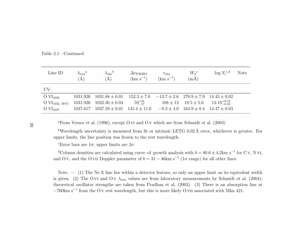
Table 2.1—Continued

Line ID λresta λobs

b ∆vFWHM vobs Wλc log Ni

c,d Note

(A) (A) (km s−1) (km s−1) (mA)

UV:

O VI1032 1031.926 1031.88 ± 0.01 152.3 ± 7.0 −13.7 ± 2.6 270.9 ± 7.9 14.43 ± 0.02

O VI1032, HVC 1031.926 1032.30 ± 0.04 59+31−17 108 ± 12 18.5 ± 5.6 13.18+0.12

−0.16

O VI1037 1037.617 1037.59 ± 0.01 145.4 ± 11.6 −9.3 ± 4.0 164.9 ± 8.4 14.47 ± 0.03

aFrom Verner et al. (1996), except Ovi and Ov which are from Schmidt et al. (2004)

bWavelength uncertainty is measured from fit or intrinsic LETG 0.02 A error, whichever is greater. For

upper limits, the line position was frozen to the rest wavelength.

cError bars are 1σ; upper limits are 2σ.

dColumn densities are calculated using curve–of–growth analysis with b = 80.6± 4.2km s−1 for Cv, Nvi,

and Ov, and the Ovii Doppler parameter of b = 31 − 46km s−1 (1σ range) for all other lines.

Note. — (1) The Ne X line lies within a detector feature, so only an upper limit on its equivalent width

is given. (2) The Ovi and Ov λrest values are from laboratory measurements by Schmidt et al. (2004);

theoretical oscillator strengths are taken from Pradhan et al. (2003). (3) There is an absorption line at

−760km s−1 from the Ov rest wavelength, but this is more likely Ovii associated with Mkn 421.

39

Fig. 2.1.— Portions of the Mkn 421 Chandra LETG spectrum (points) and the

best–fitting model (histogram). Absorption lines at z ≈ 0 are labeled, and vertical

tick marks indicate absorption from the z = 0.011 (solid) and z = 0.027 (dotted)

intervening WHIM filaments (Nicastro et al. 2005a).

40

Fig. 2.2.— FUSE spectrum of Mkn 421 around the O VIλλ1032, 1037 A absorption

doublet (histogram). The dark curve shows the best–fit model with (solid line) and

without (dotted line) the 1032 A HVC included. The inset plot shows the best–fitting

Galactic (large Gaussian) and high–velocity (small Gaussian) components for the

1032 A line, plotted against velocity relative to the Ovi rest wavelength.

41

Fig. 2.3.— Contours of allowed NOVII and b for the Ovii Kα (yellow), Kβ (red),

and Kγ lines. Shaded regions depict the 1σ errors on Wλ, with the best-fit Wλ line

in the center of each region. The overlap between these three regions 2σ limits of

24km s−1 < b < 55km s−1; the blue box depicts the 1σ ranges in log(NOVII) and b.

Also labeled on the top axis is log Tmax, the maximum temperature for a given b value.

42

Fig. 2.4.— Contours of allowed NOVI and b for the Ovi 1032 A (green), 1037 A

(red), and putative Kα 22 A (yellow) lines. Contour (a) is derived from the 1032 A

OviLV equivalent width while (b) is from the measured FWHM; the intersection

between the two green contours provides a tight constraint of b = 80.6 ± 4.2km s−1

and log NOVI(cm−2) = 14.432 ± 0.016 for the OviLV (shown as the blue cross). Note

that the Ovi Kα transition predicts NOVI about 0.5 dex higher than the UV line,

and this discrepancy cannot be explained by saturation.

43

Fig. 2.5.— Contours of constant abundance ratios for X-ray and UV oxygen

absorption lines. Vertical bars denote the 2σ range of temperatures inferred from

the abundance ratio at each step in log ne; the black cross shows the “overlap” region

between these contours. The horizontal dashed line is the 2σ upper limit on the

temperature of the Ovii absorber from the Doppler parameter measurement.

44

Fig. 2.6.— Same as Figure 2.5, but for ratios of several different ion abundances

to Ovii: OviKα (green), Oviii (red), Cvi (blue), Ne ix (cyan), and Nvii (dotted

black region). The black cross shows the range of log T and log ne derived from

the Oviii/Ovii and OviKα/Ovii ratios. Assuming solar abundances, the OviKα

and Ne ix contours are inconsistent for log ne ∼> −5, while all other ratios (except

OviKαOvii) are consistent at log ne ∼> −4.5. High–density models agree with the

data only if the OviKα measurement is disregarded.

45

Fig. 2.7.— Same as Figure 2.6, showing how a neon abundance shift of [Ne/O]= 1

produces better agreement in the low–density regime.

46

Fig. 2.8.— Models of ionic column density ratios for ions likely to arise in the Galactic

ISM (assuming pure collisional ionization). Calculated ratios are shown as thin lines

with ±2σ measurements overplotted (thick segments). Upper limits are shown as

dashed lines, and the temperature ranges derived from the different ion ratios are

shown in the lower panel.

47

Fig. 2.9.— Same as Figure 2.8, for the ions likely originating in an extragalactic

medium, with log ne = −3.9. Solar abundances relative to oxygen are assumed, and

all calculated ratios are relative to NOVII. The low–density case produces a consistent

temperature solution of T ≈ 105.7 K (from the overlap between the Oviii and OviKα

bold regions), and [Ne/O] must be supersolar.

48

Fig. 2.10.— Same as Figure 2.9 but assuming high density with only collisional

ionization. This produces a consistent solution with solar abundances but the

temperatures implied by the Oviii/Ovii and OviKα/Ovii ratios are inconsistent.

49

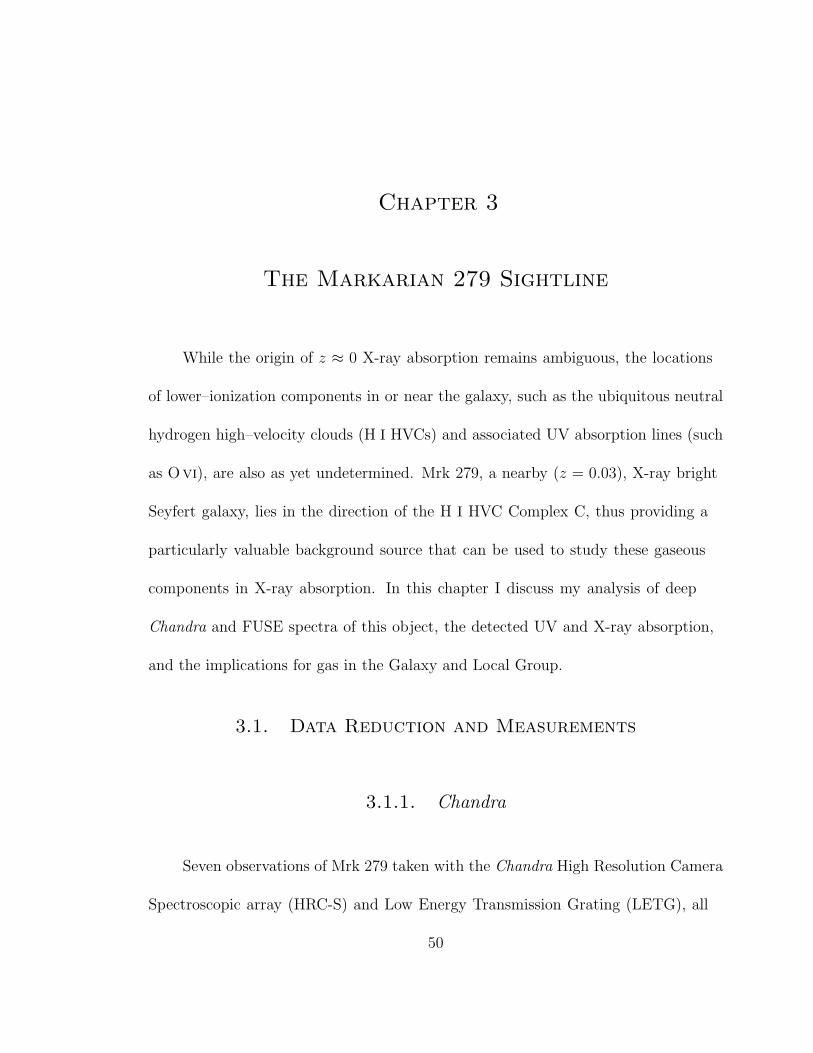
Chapter 3

The Markarian 279 Sightline

While the origin of z ≈ 0 X-ray absorption remains ambiguous, the locations

of lower–ionization components in or near the galaxy, such as the ubiquitous neutral

hydrogen high–velocity clouds (H I HVCs) and associated UV absorption lines (such

as Ovi), are also as yet undetermined. Mrk 279, a nearby (z = 0.03), X-ray bright

Seyfert galaxy, lies in the direction of the H I HVC Complex C, thus providing a

particularly valuable background source that can be used to study these gaseous

components in X-ray absorption. In this chapter I discuss my analysis of deep

Chandra and FUSE spectra of this object, the detected UV and X-ray absorption,

and the implications for gas in the Galaxy and Local Group.

3.1. Data Reduction and Measurements

3.1.1. Chandra

Seven observations of Mrk 279 taken with the Chandra High Resolution Camera

Spectroscopic array (HRC-S) and Low Energy Transmission Grating (LETG), all

50

taken in May 2003 and totaling 340 ks of exposure time, were available in the

Chandra archive. Each of these data sets was processed, and instrument response

files built, using the standard data reduction threads for HRC-S/LETG1 with

version 3.3 of the Chandra Interactive Analysis of Observations (CIAO) software

and Chandra Calibration Database version 3.2.0. Since the HRC-S does not have

sufficient energy resolution to distinguish LETG spectral orders, higher orders

can increase the apparent flux at long wavelengths2. This effect was mitigated by

including response files for orders −6 through +6 in our analysis; the inclusion

of orders beyond these had an insignificant effect on the computed instrumental

response.

The seven observations were coadded for a final (unbinned, with ∆λ = 0.0125 A)

signal–to–noise ratio of S/N ≈ 6.5 near 22A. We used the spectral fitting program

Sherpa to fit a power law and foreground Galactic absorption to the spectrum

over 10 − 100 A band (excluding the 49 − 57.5 A and 60.5 − 67.5 A chip gap

regions). The relative Galactic abundances of carbon, nitrogen, oxygen, and neon

were left as free parameters in order to produce a better fit around the absorption

edges. A power–law slope of Γ = 2.3 and equivalent hydrogen column density of

(1.78± 0.03)× 1020 cm−2 is derived, agreeing reasonably well with the Elvis, Wilkes,

& Lockman (1989) value of 1.64 × 1020 cm−2 near this sightline. The best–fit

abundances of N and Ne were approximately zero, oxygen equal to the solar value,

1Available at cxc.harvard.edu/threads/gspec.html

2See cxc.harvard.edu/ciao/threads/hrcsletg orders/

51

and carbon 0.15 solar, though we re–emphasize that these do not reflect actual

Galactic abundances but rather provide a better fit near absorption edges where

the calibration is uncertain. A few weak, broad residuals remained afterward,

probably due to calibration uncertainties or source variability; these were corrected

by including four broad Gaussians in the source model (analogous to the technique

described in Nicastro et al. 2005a).

Once the continuum was established, we visually searched the spectrum in

∼ 3 A windows for narrow (unresolved) absorption lines, fitting each one with a

Gaussian. Although several strong lines such as Cvi, Ovii, and Nvii are apparent

at the AGN redshift (z = 0.03), at z = 0 (v ∼< 700 km s−1) only Ovii Kα λ21.602 A

is unambiguously detected at 21.619 ± 0.009A (v = 236 ± 125 km s−1) with an

equivalent width of 26.6 ± 6.2 mA. Upper limits were measured for the Ovii Kβ

line as well as several other ionic species of interest; these measurements are listed

in Table 3.1. Although they are included in the model to improve consistency, the

absorption intrinsic to Mrk 279 and the Galactic interstellar O I lines are not the

focus of this work and will not be discussed further. The resulting fit and residuals

are shown in Figure 3.1 (and a zoomed–in figure near the Ovii wavelength in

Figure 3.2); with a reduced χ2 value of 0.89, the model appears to fit the data quite

well.

The Chandra HRC-S/LETG wavelength scale is uncertain for several reasons,

primarily because of non–linearities resulting from bad amplifiers on the HRC-S

52

detector3. While the newly–released CIAO 3.3 software includes a routine to correct

these non–linearities and has reduced the dispersion in wavelength errors to ∼ 6 mA

at short wavelengths in calibration spectra, this routine is in the early stages of

development and wavelengths of individual emission and absorption lines may still

be systematically skewed. However, any systematic wavelength errors should not

vary between observations as long as the telescope pointing is nominal. Furthermore,

while serious wavelength errors are known to occur around 18A, no bad amplifiers

are expected to significantly affect the dispersion relation near 21.6A (J. J. Drake

and N. Brickhouse, private communication).

To check the absolute wavelength scale near the Ovii line, we retrieved the

nearest HRC–S/LETG calibration observation of the X-ray bright star Capella

(observation 3675, taken on 2003 September 28) from the Chandra archive and

reprocessed the data in exactly the same manner as the Mrk 279 data. The

wavelength of the strong Ovii emission line was found to be 21.606 ± 0.002A or

56 ± 28 km s−1, which is consistent with the +30 km s−1 radial velocity of Capella

as listed in the SIMBAD database4. As a separate check, we reduced the Mrk 279

Chandra data both with and without the wavelength correction routine; the

difference in the measured Ovii wavelength between the two was only 4 mA, much

lower than the statistical error on the line position. Thus, although the possibility of

3See cxc.harvard.edu/cal/Letg/Corrlam/

4simbad.u-strasbg.fr/sim-fid.pl

53

systematic wavelength errors must be kept in mind, it appears as though such effects

are insignificant compared to the statistical error on the measured Ovii wavelength.

3.1.2. FUSE

Mrk 279 was observed four times with FUSE between December 1999 and

May 2003 with a total exposure time of 224 ks; all calibrated data from these

observations were obtained through the Multimission Archive at STScI website.5

To account for small shifts in the FUSE wavelength scale during the observations,

each of the constituent exposures was cross–correlated over the 1030 − 1040A range

and the relative positions of strong absorption lines were checked by eye. The data

from 18 May 2002 were not of sufficient quality to reliably perform this wavelength

calibration and were thus excluded. The coadded, wavelength-shifted spectra from

each observation were then cross–correlated with each other, scaled so that their

continuum intensities matched, combined and rebinned by five pixels (∼ 10 km s−1)

to produce a final spectrum with S/N ≈ 27 near 1032A and an effective exposure

time of 177 ks.

To account for possible systematic offsets, the absolute wavelength scale of

the final spectrum was corrected following the method employed by Williams et

al. (2005): the Galactic Si II λ1020.699 and Ar I λ1048.220 absorption profiles

5archive.stsci.edu/

54

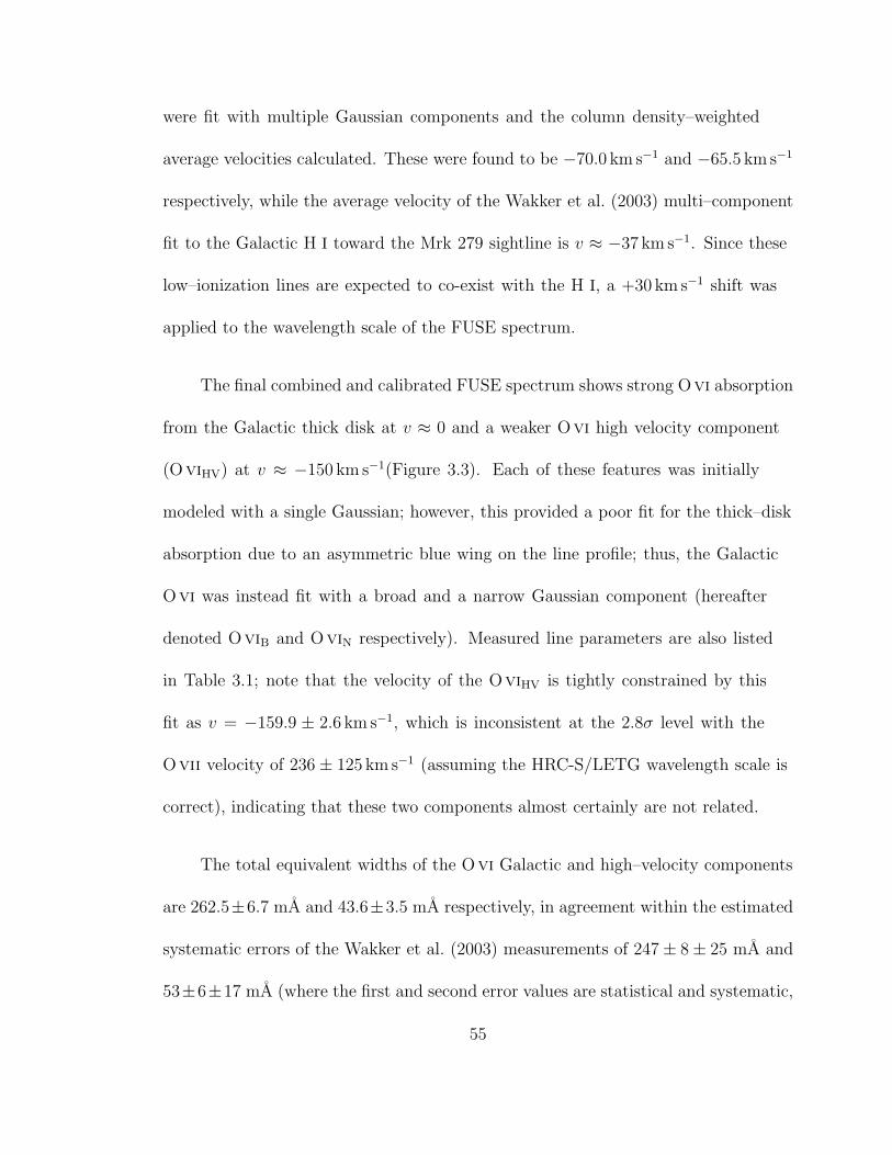
were fit with multiple Gaussian components and the column density–weighted

average velocities calculated. These were found to be −70.0 km s−1 and −65.5 km s−1

respectively, while the average velocity of the Wakker et al. (2003) multi–component

fit to the Galactic H I toward the Mrk 279 sightline is v ≈ −37 km s−1. Since these

low–ionization lines are expected to co-exist with the H I, a +30 km s−1 shift was

applied to the wavelength scale of the FUSE spectrum.

The final combined and calibrated FUSE spectrum shows strong Ovi absorption

from the Galactic thick disk at v ≈ 0 and a weaker Ovi high velocity component

(OviHV) at v ≈ −150 km s−1(Figure 3.3). Each of these features was initially

modeled with a single Gaussian; however, this provided a poor fit for the thick–disk

absorption due to an asymmetric blue wing on the line profile; thus, the Galactic

Ovi was instead fit with a broad and a narrow Gaussian component (hereafter

denoted OviB and OviN respectively). Measured line parameters are also listed

in Table 3.1; note that the velocity of the OviHV is tightly constrained by this

fit as v = −159.9 ± 2.6 km s−1, which is inconsistent at the 2.8σ level with the

Ovii velocity of 236 ± 125 km s−1 (assuming the HRC-S/LETG wavelength scale is

correct), indicating that these two components almost certainly are not related.

The total equivalent widths of the Ovi Galactic and high–velocity components

are 262.5±6.7 mA and 43.6±3.5 mA respectively, in agreement within the estimated

systematic errors of the Wakker et al. (2003) measurements of 247 ± 8 ± 25 mA and

53±6±17 mA (where the first and second error values are statistical and systematic,

55

respectively). As was the case for the Mrk 421 sightline (Williams et al. 2005),

our fitted Galactic+HVC Ovi equivalent width agrees quite well with the Wakker

et al. (2003) direct–integration value but our measurement of the OviHV strength

is somewhat lower and Galactic absorption higher; this is most likely because our

method better accounts for blending between the Galactic and high–velocity Ovi in

cases where distinct absorption components are evident (as discussed in more detail

in Williams et al. 2005).

3.2. Analysis

3.2.1. Doppler Parameters and Column Densities

In order to derive physical properties of the observed absorption, it is necessary

to first convert the measured equivalent widths into ionic column densities Ni. This

requires knowledge of the Doppler parameter b, since at a fixed column density Wλ

decreases for lower values of b. However, the nominal LETG resolution of 0.05A

(∼ 700 km s−1 at 21A) precludes direct measurement of the Ovii line width. A

method similar to that employed in Williams et al. (2005) is thus used to place

limits on the Ovii Doppler parameter using the measured equivalent width of the

Ovii Kα line and the upper limit on Ovii Kβ. Equivalent widths and FWHM

values for each transition were calculated (assuming a Voigt absorption profile) over

56

a grid of NOVII and b, and the tracks in the NOVII − b plane consistent with each

measured 2σ equivalent width limit are plotted in Figure 3.4.

Determining the ranges of NOVII and b for which the measured column densities

are consistent with each other (i.e. the area over which the Kα and Kβ tracks

“overlap”) is more complicated. In the Mrk 421 data the first three lines in the Ovii

K–series were individually detected at ≥ 3σ confidence. In that case, the differences

between pairs of predicted NOVII values (and the joint errors on the differences) were

calculable, allowing easy determination of the region over which the three transitions

predicted consistent NOVII and b values. In the case of Mrk 279, however, this same

method cannot be used because while the Ovii Kα line has been detected, only an

upper limit is available for the Kβ line.

However, since the absorption line properties for various column densities and

Doppler parameters are known, limits on these quantities can be determined using

the Chandra spectrum itself. For each point in the NOVII − b plane, Ovii Kα and

Kβ absorption lines with the calculated Wλ and FWHM values were added to the

best–fit continuum model, and the χ2 statistic calculated using the “goodness”

command in Sherpa. Over the calculated parameter ranges, the minimum χ2

point was on the b = 200 km s−1 boundary. Since the Kβ line was completely

undetected (with a best–fit amplitude near zero), the χ2 value asymptotically

approaches a minimum as b increases. We thus assumed a minimum χ2 value from

a fit with a fixed unsaturated line ratio (Wλ(Kβ) = 0.15 ∗ Wλ(Kα)) and calculated

57

∆χ2 = χ2(NOVII, b) − χ2min for every point. The 95% confidence interval (∆χ2 < 6)

determined with this method is shown in Figure 3.4; at this confidence level all

Doppler parameters between 24 < b < 74 km s−1 are ruled out.

Although these curve–of–growth diagnostics can in principle also be applied

to the UV Ovi λλ1032, 1038 absorption doublet, it is typically more difficult

because few Galactic Ovi sightlines are sufficiently saturated to significantly affect

the doublet line ratio; additionally, the close proximity of the 1037A line to other

Galactic absorption features makes deblending difficult (Wakker et al. 2003; Williams

et al. 2005). However, since the Ovi λ1032 line is fully resolved in the FUSE

spectrum, the measured line width is highly sensitive to b while the equivalent width

traces NOVI. While Wλ decreases for a saturated line of a fixed column density,

the observed FWHM increases from the unsaturated value of FWHM = 1.665b. To

account for these saturation effects, we computed Ovi λ1032 equivalent widths and

FWHM values over a grid of NOVI and b. Regions for which the FWHM and Wλ

measurements are consistent with predicted values are shown for both OviB and

OviN in Figure 3.5; since the FWHM and Wλ regions overlap nearly orthogonally,

strong constraints are placed on the column density and velocity dispersion of the

Ovi–bearing gas. None of the Ovi broad, narrow, or high–velocity components

are significantly saturated, with derived Doppler parameters of 61.5 ± 3.5 km s−1,

38.8 ± 2.8 km s−1, and 32.0 ± 4.6 km s−1 (1σ errors) respectively.

58

All Ovi component Doppler parameters are inconsistent with the upper allowed

range (b > 74 km s−1) determined from the Ovii ratios, and only the OviHV is

marginally consistent with the lower Ovii range (b < 24 km s−1). This indicates that

the majority of the v ≈ 0 Ovi cannot originate in the same phase as the observed

Ovii absorption. Although at first glance it appears possible for the OviHV and

Ovii to coexist, the velocity separation of the Ovii and OviHV (as discussed

in §3.1.2) makes this interpretation unlikely; additionally, the large Ovii/OviHV

column density ratio (NOVII ∼> 17.7; Figure 3.4) requires high temperatures which

are in turn ruled out by the low b value (discussed further in the following section).

It is also possible that the thick–disk Ovi consists of only one component with a

non–Gaussian shape, in which case the actual velocity dispersion could be larger.

Approximating the low–velocity Ovi with a single Gaussian component yields

b ≈ 75 km s−1— barely consistent with the 95% lower limit on the Ovii Doppler

parameter. We thus conclude that the Ovii most likely does not coexist with any of

the measured Ovi components.

3.2.2. Temperature and Density Diagnostics

The derived ionic column density ratios (and upper limits thereupon) can be

used to determine the physical state of the absorbing medium. Since the extent, and

hence the density, of the absorber is unknown, we cannot assume a priori whether or

not photoionization from the Galactic or extragalactic background plays a significant

59

role in the ionization balance of the medium. Specifically, in a higher–density, hot

medium (such as a Galactic corona), collisional ionization would be the dominant

process by far, while in a low–density WHIM scenario photoionization is expected to

play a significant role. Including the effects of photoionization along with collisional

ionization is crucial in order to most accurately determine the state of the gas (cf.

Nicastro et al. 2002; Mathur et al. 2003; Williams et al. 2005).

We used version 05.07 of the ionization balance code Cloudy (Ferland et

al. 1998) to calculate ionic abundances for all measured elements over a grid of

T = 104.5−107.4 K and ionization parameters log(U) = −6.3 to 0.7 (where U = nγ/ne

is the ratio of the number densities of ionizing photons and electrons in the plasma),

with a step size of 0.1 dex in both log T and logU . The Sternberg et al. (2002)

fit to the metagalactic radiation field was assumed; this is based on the observed

background from infrared to X-rays (except for the unobservable radiation near

the Lyman limit, which is taken from the theoretical model of Haardt & Madau

(1996)). The normalization of this background corresponds to electron densities of

ne = 10−7 − 1 cm−3 over the calculated log(U) range — i.e., log(ne) = −6.3− log(U).

As equivalent widths of different transitions from the same ion can be used

to place limits on the absorber’s velocity dispersion and column density (§3.2.1),

any measured column density ratio defines a track in the log T − log U plane. The

overlap between two or more such tracks (derived from different ion ratios) can

then be used to place constraints on the gas temperature and density. Although in

60

principle the ratio between any two ionic species can be employed, column density

ratios between different ions of the same atomic species are metallicity–independent

and hence produce the strongest diagnostics. Since only Ovii is strongly detected at

z = 0 in the Mrk 279 Chandra spectrum and Ovi, Ovii, and Oviii together provide

strong temperature and density constraints (Mathur et al. 2003), we focus primarily

on these ions.

A limit on NOVIII can be easily determined from the Oviii equivalent width

upper limit and assuming the Ovii Doppler parameter; however, including the Ovi

column density is less straightforward due to the presence of multiple components.

Since the Ovii Doppler parameter is inconsistent with both of the broad v ≈ 0 Ovi

components, there are two likely possibilities: (1) the Ovii Doppler parameter is

actually in the lower range (b < 21 km s−1) and the Ovii is associated with the

OviHV, or (2) the Ovi absorption produced by the Ovii–bearing gas is too weak

to be detected in our FUSE spectrum, so only an upper limit on NOVI can be used

in this analysis. The former case is highly unlikely — not only is the centroid of

the Ovii line inconsistent with the velocity of the OviHV, but such a low Doppler

parameter requires extremely high Ovii column densities (NOVII ≈ 1018 cm−2).

This in turn produces an extremely large NOVII/NOVI ratio which requires high

temperatures (T > 107.4 K, the upper limit of our calculation). Since the OviHV

Doppler parameter implies a maximum temperature of Tmax ∼< 106 K, such an

association appears impossible.

61

If, instead, the associated Ovi absorption is too weak to be detected, then this

absorption most likely takes the form of a broad (b ∼> 80 km s−1, from the Ovii b

limit) absorption line superposed on the v ≈ 0 Ovi. Such a line was included in the

FUSE spectrum fit and 2σ upper limits calculated for a velocity dispersions of 100

and 200 km s−1. The temperatures and densities consistent with the Oviii/Ovii

and Ovi/Ovii upper limits for these values of b are shown in Figures 3.6 and 3.7

respectively. The Oviii/Ovii ratio sets an upper limit of log T ∼< 6.3 and a minimum

density of 10−6 cm−3 in both cases. For b = 100 km s−1 the limits set by NOVI/NOVII

are inconsistent with the NOVIII/NOVII ratio, but for b = 200 km s−1 the contours

begin to overlap with 5.9 < log T < 6.3 and log ne > −5.1. Thus, if the Ovii is

associated with a broad undetected Ovi component, a large Doppler parameter is

required to reconcile the oxygen ion ratios. This, along with the inferred temperature

and density limits, are both consistent with expectations for the local WHIM, though

the large velocity dispersion compared to the upper temperature limit derived from

the Oviii/Ovii ratio indicates that the line broadening is primarily nonthermal.

Although a similar analysis can be performed with the Nvii/Ovii and

Ne ix/Ovii ratios, the derived limits are in all cases weaker than those set by the

Oviii/Ovii upper limit and have been excluded from Figures 3.6 and 3.7 for the

sake of clarity.

62

3.2.3. The AGN Warm Absorber

The Chandra spectrum of Mrk 279 shows strong Ovii, Oviii, Cvi, and Nvii

absorption at a redshift consistent with the AGN (z = 0.03). It is thus possible

that the Ovii absorption line at z = 0 is contaminated, either by Ovii outflowing

from Mrk 279 or from another absorption line at z = 0.03. The former scenario is

probably not the case since this would require both an unlikely coincidence of the

outflow velocity with the AGN redshift (v ≈ 9000 km s−1). To check the latter case,

we used the PHASE model (described by Krongold et al. 2003) to fit the intrinsic

absorption in a self–consistent manner. With this fit we found that the redshifted

Nvii Kβ line falls at 21.5A, near the Ovii Kα rest wavelength but well outside the

line profile, and is weak enough that its effect on the Ovii Kα equivalent width

measurement is most likely negligible. No other warm–absorber lines are expected

near 21.6A for outflow velocities between zero and 9000 km s−1; thus, the z = 0 Ovii

measurement is unlikely to be contaminated by any lines from the warm absorber.

The details of the warm absorber model are the subject of a forthcoming paper

(D. L. Fields et al., in preparation) and will not be discussed further here.

63

3.3. Discussion

3.3.1. Comparison to the Mrk 421 Sightline

Although the quality of the Mrk 279 Chandra spectrum is far lower than that

of Mrk 421 (Williams et al. 2005), the differences between the local absorption

seen along the two lines of sight are striking. While the velocity of the Mrk 421

Ovii absorption is near zero and thus cannot be distinguished from the low– and

high–velocity Ovi seen in the spectrum, the Mrk 279 Ovii and OviHV velocities

are significantly different. Furthermore, the derived Doppler parameters of the

Ovii absorption along these sightlines — 24 < b < 55 km s−1 and b > 74 km s−1 for

Mrk 421 and Mrk 279 respectively — differ substantially. In both cases association

of the Ovii with any Ovi component is ruled out and the derived temperature,

density, and column density limits are consistent with each other (though with large

errors). However, the strong discrepancy between the velocity dispersions of the two

absorbers suggests that their origins may differ. Such a difference in origin may not

be surprising, given the large (∆l ≈ 60◦) separation between the two sightlines.

3.3.2. Origin of the Absorption

The unique properties of the absorption components along the Mrk 279 sightline

provide some tantalizing clues as to the origin of the local host gas. Taking all

64

components into account, this sightline exhibits high negative–velocity H I emission

(Complex C), Ovi absorption at a similar velocity, and broad, possibly redshifted

Ovii absorption. If Complex C is indeed nearby WHIM gas that has cooled and is

falling onto the Galaxy (e.g. Miville–Deschenes et al. 2005), then its presence could

indicate the presence of a large–scale WHIM filament in the same direction. In

this interpretation, the large nonthermal Doppler parameter of the Ovii absorption

could be a result of velocity shear, due either to the Hubble expansion over a

scale of ∼ 3 Mpc (with a corresponding density of 10−5 − 10−4.5 cm−3, assuming

b = 200 km s−1, pure Hubble broadening and a metallicity of 0.1 − 0.3× solar) or

the natural velocity distribution expected from infalling gas, or a combination of

both. The negative–velocity H I would then be gas that has “broken off” from the

filament and is now falling onto the Galaxy, with the Ovi at the same velocity

representing the cooling component of the gas. The velocity of the local standard of

rest is approximately perpendicular to the CMB rest frame in this direction, so no

significant additional velocity shifts are expected in an IGM scenario.

Such a picture is consistent with the general picture of galaxy formation and

accretion of gas onto galaxies from the IGM, and the temperatures and densities

inferred from the X-ray absorption are consistent with those expected from the

WHIM. However, unlike the Mrk 421 sightline, the simulations of Kravtsov et al.

(2002) do not predict high column densities of Ovii in this direction (though this

may be due to the limited resolution of the simulations). Furthermore, aside from

65

Complex C there are no known structures in this direction that might indicate the

presence of a local filament — Wakker et al. (2003) note that the Canes Venatici

Galaxy Grouping is centered on this sightline at v ≈ 2400 km s−1, but this is far

higher than the velocity of the Ovii absorption.

Given these caveats and the large uncertainties on the X-ray measurements

(indeed, only one z = 0 absorption line has been strongly detected), the absorption

could also originate locally in hot Galactic halo or coronal gas. As discussed

previously, such an origin would require the Ovii to be a completely separate

component from any of the other observed components (H I, low– and high–velocity

Ovi) along this line of sight. Of course, there is also the possibility that the Ovii

absorption actually consists of multiple unresolved components, in which case a

multiphase solution may reconcile the discrepancy with the Ovi absorption. All line

ratio calculations were performed under the assumption of ionization equilibrium,

so nonequilibrium scenarios could provide substantively different predictions as

well. More detailed modeling and simulations of both the Galactic and IGM gas

distributions will be necessary to determine which scenario is most likely, and most

consistent with the data.

66

3.4. Conclusions

Long–duration Chandra grating observations of the bright AGN Mrk 279 reveal

the presence of strong Ovii Kα absorption at a redshift consistent with zero. A

FUSE spectrum of the same source shows several additional Ovi components at

velocities near zero. Through kinematic, curve–of–growth, and ionization balance

modeling, we conclude the following:

1. A direct χ2 analysis of the Chandra spectrum coupled with absorption

line models constrains the Doppler parameter of the Ovii absorption to

be b > 74 km s−1 and b < 24 km s−1. This latter range is unlikely due to

the extremely high Ovii column densities required to produce the strong

absorption feature.

2. The Ovii Doppler parameter limits are inconsistent with the measured b values

for any of the v ≈ 0 Ovi absorption components. Additionally, the centroid

of the Ovii Kα line is inconsistent (at the 2.5σ level) with that of the OviHV,

indicating that the Ovii is not associated with any local Ovi component.

3. If the Ovii absorption is associated with a broad, undetected Ovi absorption

line, then a large Doppler parameter (b ≈ 200 km s−1) is required to provide

a single–phase solution for the Ovi, Ovii, and Oviii column densities. This

large value of b could be a result of either microturbulence, velocity shear from

67

infalling gas, or broadening due to the Hubble expansion over a path length

of a few Mpc. If the line is purely Hubble–broadened, at b = 200 km s−1 a

pathlength of 3 Mpc and density of log n ≈ −5 is implied (assuming an oxygen

abundance of 0.3 times solar).

4. The large velocity dispersion, possible redshift, and lack of association with any

Galactic absorption components (as well as the proximity of HVC Complex

C) indicates that this X-ray absorption may be from a large–scale nearby

WHIM filament; however, a Galactic corona origin cannot be ruled out with

the current data.

68

ID λresta λobs

b ∆vFWHM vobs Wλc log Ni

c,d Note

(A) (A) ( km s−1) ( km s−1) (mA)

X-ray:

O VII Kα 21.602 21.619 ± 0.009 600+400−600 236 ± 125 26.6 ± 6.2 16.19 ± 0.19 1

O VII Kβ 18.629 18.629 · · · · · · < 7.0 < 16.24

O VIII Kα 18.969 18.969 · · · · · · < 6.5 < 15.72

N VII Kα 24.781 24.781 · · · · · · < 7.0 < 15.51

Ne IX Kα 13.447 13.447 · · · · · · < 7.3 < 15.88

UV:

OviB 1031.926 1031.75 ± 0.01 112.3 ± 5.8 −50.8 ± 3.5 169.9 ± 5.5 14.21 ± 0.02

OviN 1031.926 1031.95 ± 0.01 69.9 ± 4.4 6.7 ± 1.8 92.6 ± 3.9 13.93 ± 0.02

OviHV 1031.926 1031.38 ± 0.01 53.3 ± 7.6 −159.9 ± 2.6 43.6 ± 3.5 13.58 ± 0.04

aRest wavelengths taken from Verner et al. (1996).

bIn the cases where upper limits were found, the line positions were frozen to the rest wavelengths.

cError bars are 1σ; upper limits are 2σ.

dColumn densities for X-ray lines are calculated assuming b = 200 km s−1; for UV lines the measured

b values are used.

Note. — (1) The column density given here for the Ovii Kα line is from the equivalent width

measurement assuming b = 200 km s−1, not the χ2 method described in §3.2.1.

Table 3.1. Observed z ≈ 0 absorption lines

69

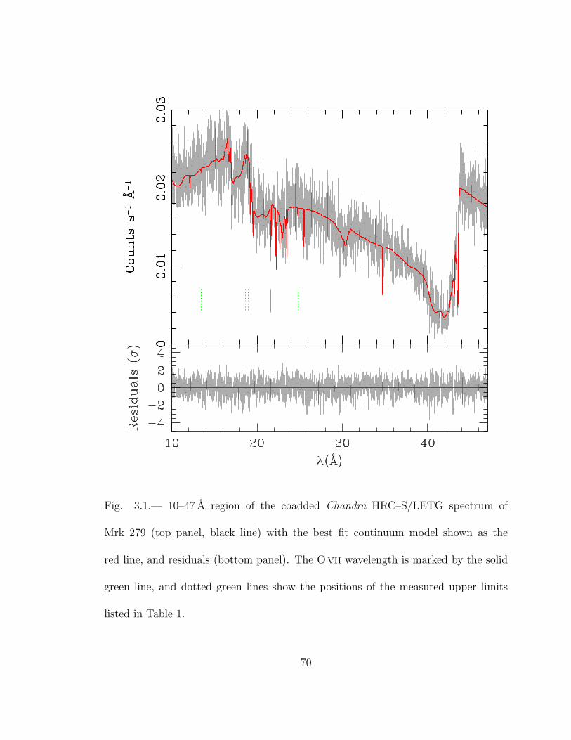
Fig. 3.1.— 10–47 A region of the coadded Chandra HRC–S/LETG spectrum of

Mrk 279 (top panel, black line) with the best–fit continuum model shown as the

red line, and residuals (bottom panel). The Ovii wavelength is marked by the solid

green line, and dotted green lines show the positions of the measured upper limits

listed in Table 1.

70

Fig. 3.2.— 18-22 A region of Figure 3.1 showing in detail the z = 0 Ovii Kα/Kβ

and Oviii Kα regions. Here, the Ovii Kβ amplitude is constrained to the minimum

(unsaturated) value, Wλ(Kβ) = 0.156 × Wλ(Kα).

71

Fig. 3.3.— Velocity relative to the local standard of rest of the local Ovii λ21.6

(top panel) and Ovi λ1032 absorption lines, with the best-fit model plotted in each

as the solid line; a representative error bar for the FUSE data points is shown at

left. Note the difference in scale between the two plots. A single–Gaussian fit to the

low–velocity Ovi absorption is also shown as the dotted line. The Ovii velocity is

inconsistent with that of the OviHV at the ∼ 2.8σ level.

72

Fig. 3.4.— Allowed values of NOVII and b given the measured Ovii Kα equivalent

width and 1σ errors (shaded region) and Ovii Kβ 2σ upper limit (dashed line).

Values of NOVII and b for which the two measurements are consistent (within 95%

confidence) are denoted by the hatched region.

73

Fig. 3.5.— Contours of constant equivalent width (solid) and FWHM (dashed) for

the low–velocity Ovi absorption, at the 1σ level. Red contours are derived from the

narrow low–velocity component and green contours from the broad component. The

inferred 1σ values of NOVI and b, as listed in Table 3.1, are shown as crosses.

74

Fig. 3.6.— Regions of consistency in the temperature–density plane for the 2σ

Oviii/Ovii and Ovi/Ovii column density ratio upper limits. Here the Ovi upper

limit is calculated from a putative Ovi absorption line with b = 100 km s−1 superposed

on the Galactic Ovi absorption. While a consistent solution cannot be found for low

velocity dispersions, at higher values of b the contours begin to overlap.

75

Fig. 3.7.— Same as Figure 3.6, but for a putative Ovi absorption line with

b = 200 km s−1.

76

Chapter 4

The PKS 2155–304 Sightline

This chapter presents a detailed analysis of the Chandra Low–Energy

Transmission Grating observations of PKS 2155–304, a bright BL Lac object at

z = 0.116. Subsets of these data were studied by Fang et al. (2002) (searching

for redshifted absorption) and Nicastro et al. (2002) (z = 0 absorption), and

here we analyze both absorption systems using all available data. This coadded

spectrum represents the second highest–quality Chandra grating observation of an

extragalactic source in terms of counts per resolution element (after Mrk 421), and

the last sightline for which potentially extragalactic, z ≈ 0 X-ray absorption lines are

likely to be detected (excluding 3C 273, which lies in the direction of a supernova

remnant). Since the physical properties of the z = 0 absorption toward Mrk 421 and

Mrk 279 differed substantially in some ways (velocity dispersion and offset from the

Ovi HVCs), a third sightline provides valuable insight into the global properties of

77

this absorption. Additionally, the relatively high redshift of PKS 2155–304 provides

a large path length over which to find intervening WHIM absorption systems.

4.1. Data Reduction and Measurements

4.1.1. Chandra

PKS 2155–304 has been observed numerous times for calibration and other

purposes with all possible combinations of the Chandra gratings and detectors. As

the strongest absorption lines previously observed have been lines from C, N, and

O at λ ∼> 18 A, for the purposes of this study we only include data from the Low

Energy Transmission Grating (LETG) since it has the highest effective area in this

wavelength regime. Chandra’s two X-ray cameras, the High Resolution Camera

(HRC) and Advanced CCD Imaging Camera (ACIS), each include separate detector

arrays for imaging (I) and grating spectroscopy (S). Although LETG observations

taken with HRC–I and ACIS–I are available in the archive, their calibration is less

certain and wavelength range more restricted than those of the spectroscopic arrays,

and so they are excluded from this analysis.

The remaining datasets include 8 employing the HRC–S/LETG instruments

and 24 with ACIS–S/LETG. Of these latter observations, however, 15 have large

pointing offsets (typically 6′ − 14′), presumably intended to characterize the off–axis

line spread function and effective area. Since the spectral resolution degrades

78

significantly at these large offsets, only the nine ACIS–S observations with |∆θ| ≤ 1.′5

are considered here. The resulting 17 observations, listed in Table 4.1, contain a total

of 483 ks of exposure time and ∼ 2100 counts per 0.05 A resolution element (CPRE)

at 21.5 A in the first LETG spectral order (253.7 ks and 880 CPRE in ACIS–S;

229.3 ks and 1200 CPRE in HRC–S). In theory this should provide roughly half the

signal–to–noise ratio obtained in the extremely high–quality LETG spectrum of Mrk

421 outburst (6000 CPRE; Nicastro et al. 2005a; Williams et al. 2005).

All datasets were fully reprocessed using the Chandra Interactive Analysis

of Observations (CIAO) software, version 3.3, with the corresponding Calibration

Database (CALDB) version 3.2.11. This CALDB version includes models for the

ACIS–S time–dependent quantum efficiency degradation as well as preliminary

corrections to the nonlinearities in the HRC–S/LETG wavelength scale. First–order

spectra were then extracted, and response matrices built, using the standard

CIAO routines. LETG spectral orders cannot be separated with HRC–S due to

this detector’s intrinsic lack of energy resolution, so the resulting spectrum is an

overlapping superposition of all orders. We thus built all HRC–S/LETG response

matrices for orders −6 to +6; past experience (e.g., Williams et al. 2006a) has shown

that this is sufficient to accurately model higher–order contamination.

The individual spectra from each instrument were then coadded, both to

allow searches by eye for intervening absorption lines and to make it easier to

1See cxc.harvard.edu/ciao/ and cxc.harvard.edu/caldb/

79

assess the goodness of fits. First, the positive and negative spectral orders from

each observation (and their corresponding response matrices) were coadded. As

PKS 2155–304 is highly variable in the X-ray band, we performed quick fits to

determine the flux near 21 A at the time of each observation. The response matrices

were then weighted by a factor of fλ(21A) × texp and coadded; these fluxes and

weights are also listed in Table 4.1. Note that, as a result of the dithering strategy

employed during observations, Chandra/LETG lacks the narrow chip–gaps and other

detector features seen in XMM–Newton grating spectra (Williams et al. 2006b);

weighting the response matrices before coaddition substantially reduces broad

residuals across the LETG band, but is not essential for narrow absorption line

measurements.

The resulting spectra were fit using the CIAO Sherpa utility. Simple powerlaw

continua (with foreground Galactic absorption as a free parameter) were fit

independently for the ACIS and HRC spectra over the 10–47 A wavelength range.

To improve the consistency of the fit near elemental edges, the foreground absorber

abundances of carbon, nitrogen, oxygen, and neon were allowed to vary. The

resulting best–fit powerlaw slopes are similar (Γ = −0.63 and −0.45 for ACIS and

HRC respectively, where fλ ≈ λ−Γ), but the Galactic absorption and abundances

vary somewhat between the two instruments, perhaps due to calibration uncertainties

or a degeneracy between Γ and NH over this restricted wavelength range. The

continuum fits for ACIS and HRC are shown in Figures 4.1 and 4.2 respectively.

80

Several absorption lines, including the Ovii, Oviii, and Ne ix Kα transitions

at z = 0, are immediately visible. These lines were modeled with narrow

(FWHM< 50 mA) Gaussian features added to the fitted continua. Since there may

be some lingering systematic uncertainties in the HRC–S/LETG wavelength scale

even with the new correction routines, wavelengths and strengths of absorption

features were first allowed to vary independently for the spectrum produced by each

instrument. Each line’s equivalent width was then determined using a joint fit to

the ACIS and HRC spectra with the requirement that the equivalent width match

between the two instruments, i.e. the normalized Gaussian line amplitudes AHRC

and AACIS (where A corresponds to the integral of the Gaussian, not the height)

were fixed according to:

fλ,HRCAHRC = fλ,ACISAACIS (4.1)

Wavelength and equivalent width errors were determined for this joint fit using

the “projection” command in Sherpa, allowing the HRC and ACIS continuum

normalizations to vary. These quantities for all measured z = 0 lines (as well as

upper limits on Ne ix and Ovii Kγ) are reported in Table 4.2, and Figures 4.3 and

4.4 show the best–fit models for all detected lines in ACIS and HRC respectively.

81

4.1.2. FUSE

The reduction and analysis of the PKS 2155–304 FUSE data were performed in

a manner nearly identical to that described for the Mrk 421 (Williams et al. 2005)

and Mrk 279 (Williams et al. 2006a) sightlines; a brief summary follows. Three

observations of PKS 2155–304totaling 120 ks were available in the FUSE section of

the Multimission Archive at STScI website.2 The calibrated data were downloaded

and individual exposures cross-correlated over the 1030–1040 A range, where many

strong absorption lines are present, to compensate for small (typically < 10 mA)

variations in the wavelength scale. The cross–correlated spectra for each observation

were then coadded, and the resulting spectra in turn cross–correlated and coadded

to produce a final coadded FUSE spectrum. The absolute wavelength scale was

checked by comparing the positions of the strong, narrow Si II λ1020.699 and Ar I

λ1048.220 absorption lines to the H I 21 cm emission. Wakker et al. (2003) find

that essentially all of the H I is concentrated in a single Gaussian component at

−4 km s−1, which matches quite well the measured Ar I and Si II velocities (−5.4 and

−5.9 km s−1 respectively, with about 0.6 km s−1statistical error). Since there may

be small (∼ few km s−1) systematic errors arising in the H I measurement and/or

the physical relation between H I and the two FUSE–measured species, we will thus

assume the FUSE wavelength calibration is correct for the purposes of this work.

2archive.stsci.edu/

82

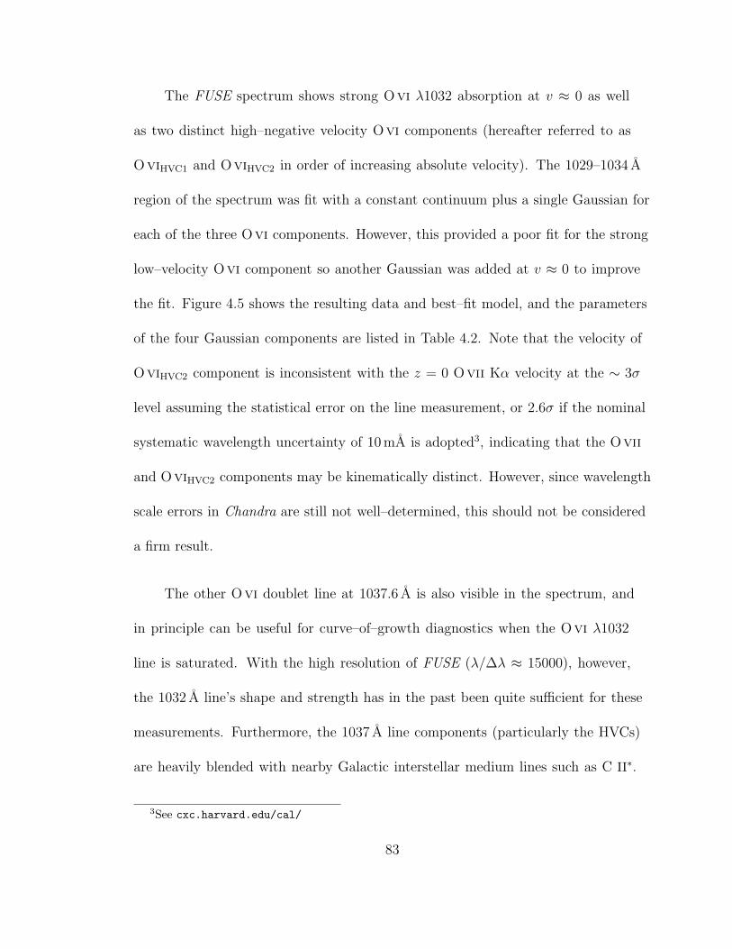
The FUSE spectrum shows strong Ovi λ1032 absorption at v ≈ 0 as well

as two distinct high–negative velocity Ovi components (hereafter referred to as

OviHVC1 and OviHVC2 in order of increasing absolute velocity). The 1029–1034 A

region of the spectrum was fit with a constant continuum plus a single Gaussian for

each of the three Ovi components. However, this provided a poor fit for the strong

low–velocity Ovi component so another Gaussian was added at v ≈ 0 to improve

the fit. Figure 4.5 shows the resulting data and best–fit model, and the parameters

of the four Gaussian components are listed in Table 4.2. Note that the velocity of

OviHVC2 component is inconsistent with the z = 0 Ovii Kα velocity at the ∼ 3σ

level assuming the statistical error on the line measurement, or 2.6σ if the nominal

systematic wavelength uncertainty of 10 mA is adopted3, indicating that the Ovii

and OviHVC2 components may be kinematically distinct. However, since wavelength

scale errors in Chandra are still not well–determined, this should not be considered

a firm result.

The other Ovi doublet line at 1037.6 A is also visible in the spectrum, and

in principle can be useful for curve–of–growth diagnostics when the Ovi λ1032

line is saturated. With the high resolution of FUSE (λ/∆λ ≈ 15000), however,

the 1032 A line’s shape and strength has in the past been quite sufficient for these

measurements. Furthermore, the 1037 A line components (particularly the HVCs)

are heavily blended with nearby Galactic interstellar medium lines such as C II∗.

3See cxc.harvard.edu/cal/

83

Since this blending can introduce additional systematic error and even slight Ovi

saturation appears to be rare (e.g. Wakker et al. 2003), we will disregard the 1037 A

Ovi line in this analysis.

4.2. Analysis

4.2.1. Doppler Parameters and Column Densities

The low resolution of the Chandra gratings compared to UV and optical

spectrographs presents unique challenges for column density measurements, since

essentially all non–quasar absorption lines are far narrower than the 50 mA

(∼ 700 km s−1 at 20 A) LETG line–spread function. The lack of line width

information prevents direct measurement of the profile shape, and hence the degree

of saturation for any given line cannot be directly determined. If multiple absorption

lines from the same ionic species are detected, however, the relative equivalent

widths of these lines can instead be used to place limits on the column density

(NOVII) and velocity dispersion (or Doppler parameter, b) of the medium.

In the case of PKS 2155–304, the Ovii Kα and Kβ lines are strongly detected,

and an upper limit is measured for the Kγ line. If all these lines were unsaturated,

the equivalent widths would scale as Wλ ≈ fijλ2 where fij is the absorption oscillator

strength. Saturation effectively decreases the equivalent widths of strong (high–fij)

84

lines while leaving weaker lines in the series more or less unaffected; thus, the ratio

Wλ(Kβ)/Wλ(Kα) increases with respect to the simple (unsaturated) proportionality

above. For Ovii, the expected Kβ/Kα equivalent width ratio is 0.156, while we

measure a ratio of 0.36±0.12, indicating that the Ovii Kα may be slightly saturated

(though it is also consistent with no saturation at the ∼ 2σ level).

To place more quantitative constraints on NOVII and b, we employ the technique

used in Williams et al. (2006a) for Mrk 279. For a grid of points in the NOVII − b

plane, equivalent widths and apparent line widths were calculated numerically (using

Voigt absorption line profiles) for the Ovii Kα, Kβ, and Kγ transitions. These lines

were then added to the continuum model in Sherpa, and χ2 calculated with the

“goodness” command, for every value of NOVII and b. Figure 4.6 shows the contours

of 1σ, 2σ, and 3σ confidence calculated in this manner.

As this figure shows, the minimum χ2 is found at b = 52 km s−1 and

log(NOVII) = 16.2, with the 1σ confidence region stretching between b = 35−94 km s−1

and log(NOVII) = 15.9 − 16.5. Additionally, another 1σ region can be found at

b < 19 km s−1 with a higher column density (log(NOVII) ≈ 17.5) required to produce

consistency with the spectrum. Such high Ovii column densities are unlikely to

be produced in a cold (Tmax ∼< 3 × 105 K), weakly photoionized medium without

producing large amounts of narrow Ovi absorption, so a low–b solution appears

unlikely. However, it is important to note that no value of b can be ruled out at the

2σ confidence level from this curve–of–growth analysis alone; as mentioned above,

85

the absorption is consistent with a completely unsaturated medium at this level,

and lower–b, higher–NOVII solutions are also possible in the regions demarcated by

the 2σ and 3σ contours in Figure 4.6. Column densities for all X-ray lines (listed in

Table 4.2) are calculated by assuming the χ2–minimizing b value above. While most

of the lines are too weak for this choice to make a significant difference in the Nion

determination, it should be kept in mind that the systematic uncertainty in NOVII

may be larger than the statistical errorbars.

Determination of these parameters for the UV Ovi λ1032 absorption is

decidedly more straightforward since the lines are fully resolved by FUSE. Since

saturation can make absorption lines broader than would be expected just from the

Doppler parameter of the gas, the measured line width cannot be used directly as a

surrogate for b. Instead, we calculate apparent Ovi FWHM values and equivalent

widths over a grid of NOVI and b, and find the regions within this grid that are

consistent with the measured ∆vFWHM and Wλ values.

Figure 4.7 shows these tracks for the low–velocity Ovi components. Contours

of constant ∆vFWHM are roughly vertical while constant Wλ are horizontal in

the unsaturated regime. In this case both Ovi1 and Ovi2 appear to be at most

weakly saturated, so the ∆vFWHM and Wλ contours overlap nearly orthogonally,

producing tight constraints on both parameters for both components. We find

that b = 41.5 ± 2.5 km s−1 and b = 51 ± 5 km s−1 for Ovi1 and Ovi2 respectively,

with column densities of log(NOVI) = 14.06 ± 0.02 and 13.94 ± 0.02. These Ovi

86

b values are fully consistent with the Ovii 1σ measurement. Since the Ovi

low–velocity lines are essentially unsaturated, and the HVCs are weaker still

(but with comparable apparent line widths), we can safely assume that they are

unsaturated; thus, we assume their b–values are directly calculable from their

FWHMs (i.e. FWHM = 2b√

ln 2 = 1.665b).

4.2.2. Temperature and Density Diagnostics

With estimates for ionic column densities, constraints on the temperature and

density of the absorbing medium can be derived. Although collisional ionization is

expected to be the dominant physical process in either the extended local WHIM or

a hot Galactic corona, photoionization from the extragalactic UV/X-ray background

is expected to significantly alter the ionization balance of the low–density WHIM (cf.

Nicastro et al. 2002). To find the most general set of conditions which can produce

the observed highly–ionized ion ratios, both collisional and photo–ionization must

be considered.

For this sightline we follow the same analysis we employed for Mrk 279 in

Williams et al. (2006a). Assuming a fixed z = 0 metagalactic ionizing background

model from Sternberg et al. (2002), the ionization parameter U = nγ(E > 13.6eV)/ne

is simply the inverse of the electron density. The ionization balance code Cloudy

(version 05.04; Ferland et al. 1998) was employed to calculate relative abundances

87

of all measured ions over a range of T = 104.5 − 107.4 K and ne = 10−7 − 1 cm−3 (or

U = 100.7 − 10−6.3) with grid spacings of 0.1 dex in each quantity, fully encompassing

the range of temperatures and densities expected in WHIM and Galactic corona

models.

With a grid of Ni computed as a function of temperature and density, the

problem can be inverted to determine which sets of T and ne are consistent with

the measured ionic column densities. However, since the local X-ray absorption is

produced in gas too hot to be detectable in neutral hydrogen emission (and Lyα

absorption at z ≈ 0 is invariably wiped out by the local interstellar medium damping

wing), no information on the overall metallicity can be derived from the data. Thus,

it is more useful to find the log T − log ne regions defined by column density ratios.

Since Ovii is by far the best–measured ion that unambiguously arises in local

warm–hot gas, we calculate all other ion column density ratios relative to NOVII.

Column density ratios of different ions of the same element are independent

of metallicity, and so depend only on the physical state of the medium. Thus,

if the Oviii and Ovii absorption arise in the same gas phase, the NOVIII/NOVII

ratio provides the most rigorous constraints on the temperature and density of the

warm–hot gas. Likewise, if any one of the four measured Ovi components exists

in this same phase, the NOVI/NOVII ratio should be consistent with an overlapping

set of temperatures and densities. Figure 4.8 shows the 2σ constraints derived

from NOVIII/NOVII and NOVI/NOVII for each of the Ovi components. Note that

88

at high densities (ne ∼> 10−4 cm−3) the temperature constraints are essentially

constant, but at lower densities photoionization becomes significant and a lower

temperature is sufficient to produce the same column density ratios. The log T

and log ne values derived from the measured NOVIII/NOVII are consistent with the

NOVI/NOVII constraints for all four components, with a typical minimum density of

ne ∼> 10−5 cm−3. Thus, association of the X-ray oxygen absorption lines with any

one of the UV Ovi components cannot be ruled out for this sightline. If the medium

is collisionally ionized, the NOVIII/NOVII ratio provides strong 2σ temperature

constraints (assuming a Doppler parameter b ≈ 52 km s−1) of 6.18 < log T < 6.36.

Similar constraints can be derived from other measured X-ray lines, though

since the ratio NCVI/NOVII depends on the relative [C/O] abundance (for example),

these constraints are more prone to systematics than those solely employing one

atomic species. Moreover, since the Ovii Doppler parameter cannot be pinned down

to better than 1σ, NOVII can vary with different b values thus significantly altering

the measured column density ratios. For the low–b solution (b < 19 km s−1), the

measured NOVIII/NOVII requires temperatures of log T ≈ 6.2. On the other hand,

such a low velocity dispersion implies a maximum temperature of log Tmax = 5.5 so

the low–b solution does not appear to be physically possible. For these X-ray line

diagnostics, we thus consider only the best–fit 1σ region of b = 52+42−35 km s−1 and a

large–velocity dispersion, low saturation (b ≈ 200 km s−1) solution.

89

Figures 4.9 and 4.10 show the constraints, for b = 52 and b = 200 respectively,

derived from the ratios of Ne ix, Cvi, and Oviii to Ovii. The column density

limits measured for Nvi and Nvii did not provide any useful constraints (i.e., they

were consistent with nearly the entire range of temperatures and densities) and were

excluded from these figures for clarity. Furthermore, the Cv ion is expected to form

in cooler gas than that producing the Ovii and Oviii absorption (most likely the

local warm ISM and/or the Galactic thick disk), and so the NCV/NOVII constraint

was also not considered for this analysis.

In the best–fit b plot (Figure 4.9), the constraints derived from all three

column density ratios overlap quite well in the collisionally–ionized density regime

(ne ∼> 10−5 cm−3). However, at a large velocity disperion (b = 200; Figure 4.10),

there is essentially no set of log T and log ne for which the three constraints overlap.

The Cvi and Ne ix lines are relatively weak and not as affected by saturation as

the Ovii, so this change is driven primarily by the decrease in NOVII at higher

velocity dispersion. It should be re–emphasized that the contours derived from NCVI

and NNeIX depend on [C/O] and [Ne/O]; however, if the abundance mixture of this

absorber is roughly solar, then the measured column densities indicate that the

previously derived Doppler parameter range (b = 35 − 94 km s−1) fit the data better

than a high–b, unsaturated medium.

90

4.2.3. z = 0.055 Absorption Reported by Fang et al.

In a previous study incorporating a subset of the data analyzed herein

(ACIS–S/LETG observation IDs 1703, 2335, and 3168), Fang et al. (2002, hereafter

F02) report the detection of an absorption line at 20.02 ± 0.015 km s−1 with

equivalent width 14.0+7.3−5.6 mA, possibly corresponding to Oviii at a velocity of

16634±237 km s−1 (z = 0.055±0.001). Several previously discovered Lyα absorption

lines and a small cluster of H I galaxies appear at a similar velocity in this direction,

so such an absorber may be indicative of intragroup medium or an associated

large–scale WHIM filament.

This absorption line is clearly visible in our coadded ACIS spectrum, but is

not visible in the HRC spectrum (Figure 4.11). A fit to the line in ACIS yields a

wavelength of 20.03 ± 0.01 A and an equivalent width Wλ = 7.5 ± 2.1 mA, both

consistent with the F02 measurement. An upper limit for a line at this wavelength

(±0.02 A, to account for possible discrepancies in the HRC/LETG wavelength

scale) was calculated and found to be Wλ < 12.5 mA (2σ confidence), so the

ACIS measurement is not ruled out by the HRC detection. Moreover, our best–fit

equivalent width is roughly half that (and hence half the Oviii column density)

measured by F02. If real, this detection would still be fully consistent (albeit with

large errors) with the predicted number of Oviii absorbers per unit redshift (F02,

Figure 2).

91

However, the existence of this line is brought into question by the higher–quality

ACIS/LETG spectrum of Mrk 421 (see Figure 4.11). In this spectrum, a weak

detector feature is seen at ∼ 19.97 A, or 50 mA from the wavelength of the feature

seen toward PKS 2155–304. The instrument model of the Mrk 421 spectrum appears

to partially compensate for this detector feature, but no such feature is seen in the

instrumental response of the PKS 2155–304 spectrum. The presence of a detector

feature near this wavelength in the Mrk 421 spectrum is worrisome, as it may be

indicative of a transient anomaly (or one that was deemed insignificant, and removed

from the instrument model before the bulk of the PKS 2155–304 observations).

Because of this, coupled with the apparent absence of other highly–ionized absorption

lines at this velocity in the new higher–quality PKS 2155–304 data, we conclude

that there is a high likelihood that the previous detection was due to a feature in the

ACIS-S/LETG system.

4.3. Discussion

4.3.1. Comparison to Other Lines of Sight

PKS 2155–304 represents the third and final Chandra data set we have analyzed

for which relatively weak (∼ 10 mA) absorption, uncontaminated by known hot

foreground gas (as in 3C 273, situated along the line of sight to a supernova remnant)

can be detected at high confidence. Although the number of such sightlines is small,

92

similarities and differences in the detected absorption are already beginning to

emerge.

Mrk 421

The Chandra LETG spectrum of Mrk 421 contains is the highest–quality

grating spectrum of an extragalactic source to date, with roughly three times the

counts per resolution element at 21 A as the PKS 2155–304 data analyzed here

(Nicastro et al. 2005a; Williams et al. 2005). Many of the ionic species seen toward

Mrk 421 (particularly Ovii, Oviii, Ne ix, and Cvi) were also detected in the

PKS 2155–304 spectrum, allowing direct comparisons to be made. In particular,

the Ovii absorption (the strongest–detected ion in both cases) shows strikingly

similar properties between the two objects–NOVII = 16.23 ± 0.21 in Mrk 421

versus 16.09 ± 0.19 in PKS 2155–304. Both Ovii absorbers exhibit consistent

velocity dispersions as well, with bOVII = 24 − 55 km s−1 (2σ limits) in Mrk 421 and

35− 94 km s−1 in PKS 2155–304 (though this latter quantity is the 1σ range, and 2σ

limits could not be determined).

One of the most surprising features of the Mrk 421 Chandra spectrum is the

presence of a weak (2.0 mA) absorption line at 22.02 A, the expected wavelength of

the Ovi Kα inner–shell transition. Even though both this transition and the 1032 A

lines should both trace the Ovi ground state, the column density derived from the

observed Kα line is a factor of ∼ 4 higher than that derived from the UV transition.

93

If this Kα transition is a better tracer of the true Ovi column density than the

UV line, then the Ovii toward Mrk 421 almost certainly arises in a low–density,

photoionized medium.

Although the Ovi λ1032 absorption strength toward PKS 2155–304 is

comparable to the Mrk 421 sightline, unfortunately the Chandra spectrum does

not have sufficient signal–to–noise to detect the Kα line. Thus, for PKS 2155–304

we cannot determine if there is the same discrepancy between the UV and X-ray

Ovi, or if the inferred Ovi Kα column density also implies a photoionized medium

along this sightline. If the Ovi Kα measurement is disregarded, then the Mrk

421 spectrum implies slightly lower–but marginally consistent–temperatures in the

collisionally ionized regime (log T = 6.1 − 6.2; 2σ limits from the Oviii/Ovii ratio)

than PKS 2155–304 (log T = 6.18 − 6.36). The lower density limit from Mrk 421

is somewhat more stringent than that derived from the PKS 2155–304 oxygen ion

ratios (log ne > −4.7 versus > −5.5), though this may again be primarily an issue of

spectral quality.

Mrk 279

The z = 0.03 Seyfert galaxy Mrk 279 is significantly less luminous than either

PKS 2155–304 or Mrk 421, but it was observed sufficiently long with Chandra

HRC–S/LETG to produce a reasonably high–quality spectrum in which strong

z = 0 Ovii Kα absorption was detected (Williams et al. 2006a). Two features of

94

this absorption were particularly interesting: (1) the unusually strong Ovii Kα

absorption (Wλ = 26.6 ± 6.2 mA), coupled with a tight upper limit on the Kβ line,

indicated that the absorption was best described as an unsaturated medium (with

a 2σ lower limit of b > 77 km s−1 on the Doppler parameter); and (2) the Ovii

absorption appears slightly redshifted, making its velocity inconsistent with the Ovi

HVC’s negative velocity at the 2.5σ level.

As previously mentioned, the velocity of the Ovii toward PKS 2155–304

appears to be inconsistent with the OviHVC2 velocity at the 2.6σ level, assuming

the nominal HRC–S/LETG wavelength scale uncertainty of 10 mA. Until systematic

errors in the wavelength scale can be better understood, however, this should not be

taken as a definitive result. Moreover, while the Ovii toward Mrk 279 could not

be directly associated with either low–velocity Ovi component since their velocity

dispersions were significantly different, such an association cannot be ruled out in

the PKS 2155–304 absorption: all of the Ovi Doppler parameters fall within the 1σ

b confidence interval found for the Ovii absorption.

Temperature and density constraints on the z = 0 absorption toward Mrk 279

and PKS 2155–304 are consistent with each other, though this is not surprising–since

the quality of the Mrk 279 spectrum is lower, only an upper limit on temperature

and a lower limit on density could be derived.

95

4.3.2. Where is the Absorption?

In principle, the degree of photoionization of an absorbing medium (and hence

an estimate of the gas density) can be derived from ionic column density ratios

(§4.2.2). However, in the case of PKS 2155–304, the errors are large enough that no

upper limit on the gas density can be found, i.e. it is fully consistent with collisional

ionization. Depending on the assumptions made (in particular, which if any of the

Ovi components are associated with the Ovii and Oviii), the minimum density

of this medium appears to be log ne ∼> −5.5. The best–fit Ovii column density is

log NOVII = 16.09 and Ovii is by far the dominant ionization state in this medium.

If the gas has a metallicity of 0.3× solar (comparable to that observed in the diffuse

intracluster medium), then the total hydrogen density is roughly log NH ≈ 19.9 and

the thickness of the absorber d ∼< 1025.4 cm = 8.4 Mpc.

Thus, under a set of reasonable assumptions, the observed absorption is

consistent with an extended extragalactic medium, but within the very large errors

it is just as reasonable to associate it with a local hot Galactic corona. Although an

association between the X-ray absorber and low–velocity Ovi cannot be ruled out

from these data alone, the properties of the X-ray absorber are quite similar (again

within the errors) to those studied along the Mrk 421 and Mrk 279 sightlines. These

latter two X-ray absorbers are definitely not associated with the low–velocity Ovi

absorption arising in the Galactic thick disk, so if they indicate the presence of an

96

additional hot Galactic component, then the derived properties of the PKS 2155–304

absorber are not in conflict with the other measurements of this component.

4.3.3. Comparison to Nicastro et al. (2002)

In their study of three HRC–S/LETG observations of PKS 2155–304

(observation IDs 331, 1013, and 1704), Nicastro et al. (2002, hereafter N02) also

detected OviiKα and Kβ, Oviii, and Ne ix, albeit at lower confidence. They

also analyze FUSE data of the same sightline, but at that time only 39 ks were

available, or about one–third of the exposure time analyzed here. As it turns out,

the addition of new Chandra and FUSE data brings about significant changes in the

interpretation of the local absorption, in two important ways.

First, while N02 were able to fit the observed Ovi λ1032 line with two Gaussian

components (one low–velocity narrow line and a broader, blueshifted HVC), the

new higher–quality spectrum reveals that the “broad” component is actually two

distinct HVCs, and the narrow low–velocity Ovi is best fit with two components.

Second, while the Ovii Kβ line was previously not detected strongly enough to

place constraints on the Doppler parameter of the absorption, here the Kα and Kβ

lines hint at some degree of saturation and so the Ovii column density we employ

in our analysis is about 0.5 dex higher than that reported by N02. Both of these

effects cause a sharp decrease in the NOVI/NOVII ratio, which in turn removes the

97

need for a photoionization contribution. Indeed, when we calculate temperature

and density constraints assuming b = 200 (as N02 had done; see Figure 4.10) we

also find that a high–density, collisionally–ionized solution cannot be found without

modifications to the relative abundances. This highlights the major improvements

in diagnostic power that can be made by accumulating large numbers of counts per

resolution element, either through very long exposures or observations of especially

bright background sources.

4.4. Conclusions

Using all available Chandra LETG data on PKS 2155–304, we have analyzed in

detail the ionization and kinematic state of the warm–hot z ≈ 0 absorbing medium.

We find a Doppler parameter range of b = 35 − 94 km s−1 (1σ limits; 2σ limits could

not be found), which is consistent with the absorption seen toward both Mrk 421 and

Mrk 279 (though the best–fit value best matches the former sightline). Assuming

that the Doppler parameter lies in this range, ionic column densities of Ovii, Oviii,

Ne ix, and Cvi are consistent with collisional ionization at log T (K) = 6.18 − 6.36,

though a low–density photoionized WHIM cannot be ruled out. Unlike the other

two previously analyzed sightlines, the Ovii absorption toward PKS 2155–304 may

be associated with either one of the low–velocity Ovi λ1032 components seen in

FUSEor a high–velocity Ovi cloud at v = −130 km s−1 (though its velocity may be

98

inconsistent at the ∼ 2.5σ level with another Ovi HVC at v = −234 km s−1). The

intervening Oviii absorber at z = 0.055 reported by Fang et al. (2002) is detected

in ACIS, but may be related to an unmodelled detector feature that is seen in other

ACIS-S/LETG spectra.

It is notable that the Chandra data for this line of sight hint at a number of

interesting results (particularly the possibly low Doppler parameter) but the data

are not quite of sufficient quality to confidently confirm them. PKS 2155–304 is

quite possibly the only other source bright enough to obtain a Chandra LETG

spectrum with ∼ 6000 counts per resolution element, comparable to the Mrk 421

spectrum analyzed by Williams et al. (2005), in a reasonable amount of time. Such

a spectrum would not only allow a direct comparison of the z ≈ 0 absorption along

two lines of sight, but would also provide a path length four times larger than Mrk

421 to search for “missing baryons” in intervening WHIM filaments. With two such

systems detected in Mrk 421, a correspondingly larger number could be detected in

a PKS 2155–304 spectrum at comparable signal–to–noise. Thus, this is a case where

longer observations of this object are both attainable and have the potential for

great scientific benefit.

99

Obs ID Date texp fλ(21A)a Wib

(ks) (ks−1 cm−2 A−1)

ACIS–S/LETG

1703 2000 May 31 25.2 3.4 0.121

2335 2000 Dec 06 29.1 2.4 0.090

3168 2001 Nov 30 28.8 6.7 0.223

3668 2002 Jun 11 13.5 6.9 0.120

3707 2002 Nov 30 26.9 1.6 0.054

4416 2003 Dec 16 46.5 3.2 0.174

6090 2005 May 25 27.5 3.2 0.106

6091 2005 Sep 19 29.2 2.6 0.087

6927 2006 Apr 02 27.0 0.8 0.025

HRC–S/LETG

331 1999 Dec 25 62.7 9.7 0.514

1013 2001 Apr 06 26.6 2.9 0.065

1704 2000 May 31 25.8 3.7 0.081

3166 2001 Nov 30 29.8 8.4 0.212

3709 2002 Nov 30 13.7 2.3 0.026

4406 2002 Nov 30 13.9 2.4 0.028

5172 2004 Nov 22 26.9 1.8 0.041

6923 2006 May 01 29.9 1.3 0.032

aBackground–subtracted photon flux at 21A; the HRC–S

values are apparent fluxes including all higher orders.

bWeight factors for coadding the response matrices, calculated

as Wi = fλ,i(21A)texp,i/Σi(fλ,i(21A)texp,i).

Table 4.1. Chandra observation log

100

ID λresta λobs

b ∆vFWHM vobs Wλc log Ni

c,d Note

(A) (A) ( km s−1) ( km s−1) (mA)

X-ray:

C V Kα 40.268 40.227+?−.015 · · · −305+?

−112 11.4 ± 5.1 15.22+0.26−0.33 1

C VI Kα 33.736 33.732+.011−.007 · · · −36+98

−62 5.6 ± 2.5 15.16+0.18−0.27

O VII Kα 21.602 21.611+.002−.008 · · · 125+28

−111 11.6 ± 1.6 16.09 ± 0.19

O VII Kβ 18.629 18.618 ± .007 · · · −177 ± 113 4.2 ± 1.3 16.09+0.17−0.21

O VIII Kα 18.969 18.987+.003−.008 · · · 285+47

−126 6.7 ± 1.4 15.80+0.11−0.13

Ne IX Kα 13.447 13.451+.010−.003 · · · 89+223

−67 4.5 ± 1.1 15.83 ± 0.21

N VI Kα 28.787 28.787 · · · · · · < 8.4 < 15.39

N VII Kα 24.781 24.781 · · · · · · < 5.0 < 15.39

O VI Kα 22.019 22.019 · · · · · · < 5.7 < 15.36

O VII Kγ 17.768 17.768 · · · · · · < 5.3 < 16.71

(cont’d)

Table 4.2. Observed z ≈ 0 absorption lines

101

Table 4.2—Continued

ID λresta λobs

b ∆vFWHM vobs Wλc log Ni

c,d Note

(A) (A) ( km s−1) ( km s−1) (mA)

UV:

Ovi1 1031.926 1032.11 ± 0.01 76.4 ± 4.1 53.5 ± 2.9 120.5 ± 3.8 14.06 ± 0.02

Ovi2 1031.926 1031.85 ± 0.01 90.1 ± 8.1 −22.1 ± 2.9 98.2 ± 4.4 13.94 ± 0.02

OviHVC1 1031.926 1031.48 ± 0.01 74.2 ± 5.8 −129.7 ± 2.9 73.1 ± 4.0 13.81 ± 0.03

OviHVC2 1031.926 1031.12 ± 0.02 80.3 ± 14.5 −234.3 ± 5.8 46.6 ± 4.5 13.59 ± 0.05

aRest wavelengths taken from Verner et al. (1996), except Ovi Kα which is from the laboratory

measurements of Schmidt et al. (2004).

bIn the cases where upper limits were found, the line positions were allowed to vary within 20 mA

of the rest wavelengths. Measured wavelengths are taken from ACIS–S since its dispersion relation is

thought to have the fewest nonlinearities; however, only the statistical fit error is given in this column

(i.e., not taking into account possible wavelength scale uncertainties of up to ∼ 10 mA).

cError bars are 1σ; upper limits are 2σ.

dColumn densities for X-ray lines are calculated assuming the 1σ Doppler parameter region found in

Figure 4.6 (35-94 km s−1 for Ovii); for UV lines the measured b values are used.

Note. — (1) An upper error bar could not be formally determined for the wavelength of this line.

102

Fig. 4.1.— Chandra grating over the 10–47A range from ACIS-S/LETG with residuals

from the best–fit continuum shown in the lower panel. Several narrow absorption lines

are apparent in these residuals.

103

Fig. 4.2.— Same as Figure 4.1, showing the continuum fit for the Chandra HRC–

S/LETG spectrum.

104

Fig. 4.3.— ACIS–S/LETG data (points) and best–fit model (histogram) near each

of the six z = 0 X-ray absorption lines detected toward PKS 2155–304.

105

Fig. 4.4.— Detected z = 0 absorption lines in HRC–S; see Figure 4.3 for details.

106

Fig. 4.5.— Ovi λ1032 region of the PKS 2155–304 FUSE spectrum. The four

Gaussian components used to model the z ≈ 0 Ovi complex are labeled.

107

Fig. 4.6.— Ovii Doppler parameter and column density contours (at the 1σ, 2σ, and

3σ confidence levels) determined by simultaneously Ovii Kα, Kβ, and Kγ lines in

the joint LETG/ACIS+HRC Chandra spectrum.

108

Fig. 4.7.— Column density and velocity dispersion constraints derived from Ovi

λ1032 equivalent widths (roughtly horizontal lines) and FWHMs (vertical lines),

for the Ovi1 (solid) and Ovi2 (dashed) components. Regions of overlap, marked

with crosses, denote the approximate 1σ confidence intervals on NOVI and b for each

component.

109

Fig. 4.8.— Oxygen ion temperature and density constraints for NOVIII/NOVII and

NOVI/NOVII for each of the four measured Ovi components.

110

Fig. 4.9.— Temperature and density constraints from ion column density ratios

relative to NOVII, where column densities are derived assuming the best–fit region

near b = 50 km s−1 shown in Figure 4.6.

111

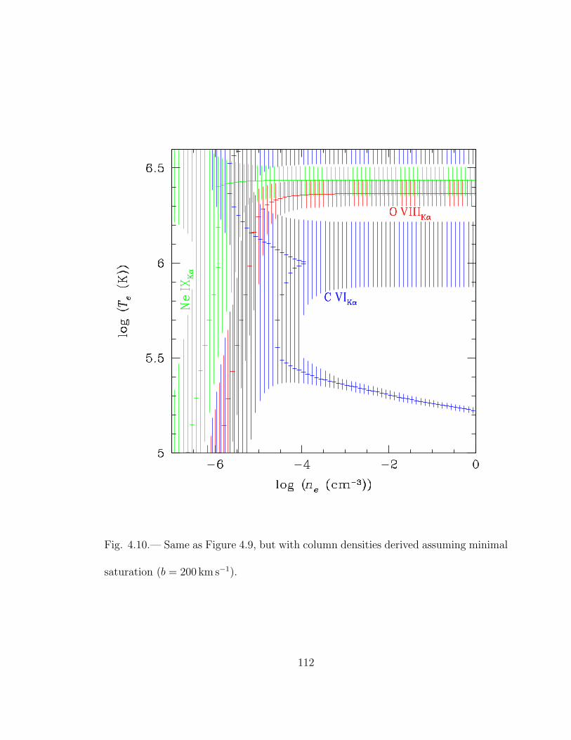
Fig. 4.10.— Same as Figure 4.9, but with column densities derived assuming minimal

saturation (b = 200 km s−1).

112

Fig. 4.11.— ACIS–S and HRC–S/LETG (top and center panels, respectively) spectra

of PKS 2155–304 near the wavelength of the z = 0.055 Oviii intervening feature

reported by (Fang et al. 2002), and the same portion of the Mrk 421 ACIS–S/LETG

spectrum. The presence of a feature near this wavelength in both ACIS–S/LETG

spectra and not in the HRC spectrum indicates that this line is most likely a detector

feature.

113

Chapter 5

Instrumental Considerations: Chandra or

XMM–Newton?

In this chapter I take a small step upwards in redshift and discuss the two

intervening WHIM filaments discovered by Nicastro et al. (2005a) through their

X-ray absorption lines in a high–quality Chandra spectrum of the blazar Mrk 421.

Although each of these two absorption systems was detected with high confidence

through multiple lines, the individual absorption lines were generally quite weakly

detected, mostly at the 2 − 4σ level. Moreover, while they employed high–quality

Chandra and FUSE data taken during exceptionally bright outbursts of Mrk 421,

the many archived XMM–Newton observations of this source were not included in

the analysis. With roughly twice the effective area of Chandra/LETG, XMM/RGS

is in principle superior for X-ray grating spectroscopy between ∼ 10 − 40 A;

however, its slightly worse resolution (approximately 60 mA FWHM, versus 50 mA

for Chandra/LETG), higher susceptibility to background flares, and multitude of

narrow instrumental features can present serious complications for WHIM searches.

114

Independent confirmation of the Chandra results with a separate instrument

like XMM is thus important. While some groups have searched for WHIM features

in a limited number of XMM Mrk 421 spectra (e.g., Ravasio et al. 2005), a complete

and systematic analysis has yet to be performed. Here I present a search for z > 0

WHIM features employing all “good” observations of Mrk 421 available in the XMM

archive, and a comparison of these results to those presented by Nicastro et al.

(2005a).

5.1. Data Reduction and Measurements

We searched the XMM archive for all Mrk 421 Reflection Grating Spectrometer

(RGS) data. Although 31 separate observations were available, 16 had pointing

offsets ∆θ ∼> 60′′ while the rest were offset by less than 15′′. Since spectral resolution

and calibration quality can degrade at large offsets, we only included those with

∆θ < 15′′. One extremely short observation (0158971101, with texp = 237 s) was

also excluded to simplify the data reduction process. Using the standard XMM

Science Analysis System version 6.5.0 routines1, RGS1 light curves were built for the

remaining 14 “good” observations (see Table 5.1), and the spectra were reprocessed

to exclude periods of high background levels and coadded. These combined, filtered

RGS1 and RGS2 spectra have effective exposure times of ∼ 440 ks and over 9 × 106

combined RGS1+RGS2 first–order counts between 10 − 36 A with ∼ 15000 counts

1See xmm.vilspa.esa.es/sas

115

per 0.06 A resolution element in RGS1 near 21 A, over twice that in the Nicastro et

al. (2005a) Mrk 421 Chandra spectrum.

We first used the spectral fitting program Sherpa2 to fit a simple power law

plus Galactic foreground absorption model to the RGS1 and RGS2 data; however,

at such high spectral quality the RGS response model does not appear to be

well–determined, and large residuals remained. For line measurements, we thus

only considered ∼ 2 A windows around each wavelength of interest, using a power

law to independently model the RGS1 and RGS2 continua within each window

and excluding the strongest narrow detector features (with typical widths of 70 mA

or less). None of the intervening absorption lines were apparent through a visual

inspection of the XMM spectrum, though several of the z = 0 lines reported by

Williams et al. (2005) could be seen clearly.

A narrow Gaussian absorption line (FWHM= 5 mA) was included in the

model for each line measurement or upper limit reported by Nicastro et al.

(2005a). When convolved with the RGS instrumental response these absorption

lines appeared broadened to the RGS line spread function (LSF) widths (typically

FWHM= 60− 70 mA; den Herder et al. 2001). The 2σ upper limits on all equivalent

widths were then calculated (allowing the central line wavelengths to vary within

the 1σ errors reported by Nicastro et al. 2005a). Since the shapes of the RGS1 and

RGS2 instrumental responses are quite different, these limits were calculated using

2cxc.harvard.edu/sherpa/

116

both a joint fit to the RGS1+RGS2 spectra as well as the individual RGS1 and

RGS2 spectra. It should be noted that wherever one RGS unit is unusable, the

total response is effectively halved, at which point it has a similar effective area to

Chandra/LETG. The resulting equivalent width limits are listed in Table 5.2.

5.2. Discussion

Figure 5.1 shows the spectral windows used to determine upper limits on the

Nicastro et al. (2005a) measured lines, with the data (black), continuum fit (blue),

Chandra measurements and limits (Nicastro et al. 2005a, red solid and dotted lines

respectively), and XMM limits (green) overplotted. In all cases, the Nicastro et al.

(2005a) measurements (or 3σ upper limits) appear to be consistent with the 2σ

upper limits we have derived directly from the XMM data, as shown in the figure and

listed in Table 5.2. The Ovii line at z = 0.027 looks as though it might be visible

in the spectrum, but this is most likely due to the weak instrumental feature at

∼ 22.1 A. For two lines (Nvii and Nvi at z = 0.027) the XMM 2σ upper limits are

approximately equal to the Nicastro et al. (2005a) best–fit measurements, but since

the Nicastro et al. (2005a) values are quite uncertain this result is still consistent.

Why, then, with 2 − 4 times the counts per resolution element, was XMM

unable to detect the intervening absorption systems seen by Chandra? Several

factors appear to have been involved in this non–detection, primarily: (1) narrow

117

instrumental features caused by bad detector columns, (2) the broader LSF as

compared to Chandra/LETG, and (3) fixed–pattern noise at long wavelengths:

1. While broad instrumental features can be taken into account by modifications

to the continuum model (as in Nicastro et al. 2005a), it is difficult or impossible

to distinguish narrow features from true absorption lines; thus, any line falling

near one of the detector features shown in Figure 5.2 can easily be lost3. This

was responsible for the non-detection of the z = 0.011 Ovii Kα line. Although

it was the strongest line reported by Nicastro et al. (2005a), its wavelength falls

directly on a narrow RGS1 feature and within the non–functional CCD4 region

on RGS2, thereby preventing this line from being detectable with either RGS.

Since 18% of the wavelength space for studying redshifted Ovii (λ > 21.6 A)

toward Mrk 421 is directly blocked by these narrow features (with this number

climbing to about 60% if resolution elements immediately adjacent to bad

columns are included), these bad columns present the single greatest hindrance

to XMM/RGS studies of the WHIM.

2. Even for lines where both RGS1 and RGS2 data are available and the

instrumental response appears to be relatively smooth, the lower resolution of

XMM contributes to the nondetectability of the weaker z > 0 absorption lines.

Figure 5.3 shows the LSFs for both XMM/RGS1 (solid) and Chandra/LETG

assuming an unresolved line with Wλ = 10 mA at 21.6 A. While the core of

3These response file data can be found at www.astronomy.ohio-state.edu/∼smita/xmmrsp/

118

the RGS1 response is ∼ 20% broader than that of the LETG, the RGS1 LSF

has extremely broad wings: only 68% of the line flux is contained within the

central 0.1A of the RGS1 LSF, as opposed to 96% for the LETG. This reduces

the apparent depth of absorption lines by about a factor of two as compared

to Chandra/LETG, severely decreasing the line detectability.

3. At long wavelengths (λ ∼> 29 A) strong fixed–pattern noise is apparent as a

sawtooth pattern in the instrumental response, strongly impeding the detection

of species such as Nvi and Cvi. Indeed, in these wavelength regimes (the

lower two panels of Figure 5.1), the Nvi and Cvi absorption lines are nearly

indistinguishable from the continuum.

5.3. Disputed Results

After its publication, this paper understandably drew some criticism from

groups affiliated with the XMM mission in general, and the RGS instrument in

particular. Kaastra et al. (2006) and Rasmussen et al. (2006, hereafter R06), two

journal–submitted papers that subsequently appeared on the astro–ph preprint

server, contested our result that the XMM lacked sufficient sensitivity to detect the

intervening WHIM filaments reported by Nicastro et al. (2005a). In fact, both claim

that the lack of an XMM detection implies that the filaments are either a statistical

fluctuation or a result of instrumental artifacts in Chandra/LETG, and that X-ray

119

absorption lines from the local WHIM have yet to be found. As Kaastra et al. (2006)

primarily focuses on a reanalysis of Chandra and XMM data while R06 directly

attempts to refute the points presented in this paper, I will primarily address the

R06 points here.

The primary claim of R06 is that custom reduction techniques, applied during

the processing of XMM/RGS data, allow narrow detector features to be modeled

to a high degree of accuracy. This would be quite an important development since,

as we described previously, such detector features prevent absorption lines at those

wavelengths from being accurately measured (or even detected in many cases). The

ability to successfully mitigate these features would open up substantially more of

the RGS wavelength range for the detection of redshifted WHIM lines.

However, perhaps the most surprising aspect of R06 is that, assuming the R06

fit is perfect, the upper limits measured for the two intervening OVII absorbers are, at

worst, in no more that weak conflict with the Nicastro et al. (2005a) measurements.

R06 presents column density upper limits calculated at the wavelengths of the two

redshifted Ovii absorption lines reported by Nicastro et al. (2005a), obtaining 90%

upper limits of NOVII < 1 and 1.1 × 1015 cm−2 for the z = 0.011 and z = 0.027

systems respectively. More stringent upper limits (< 6 × 1014 cm−2) are also

calculated when the wavelength is frozen to the value reported by Nicastro et al.

(2005a), but the error in the line position must be taken into account in order to

accurately calculate the equivalent width error–hence, the less stringent limits are

120

correct. Nicastro et al. (2005a) report measurements of (1.0 ± 0.5) × 1015 cm−2 and

(0.7 ± 0.5) × 1015 cm−2 (also 90% errorbars) for these two systems. Clearly, the R06

upper limits are consistent with the R05 measurements. It is thus apparent that R06

reached their conclusion using the more stringent, but incorrectly–calculated, upper

limits.

It should also be noted that we have presented three serious problems with

using XMM/RGS for weak absorption line studies: not only the narrow detector

features, but also the broad LSF wings and the long–wavelength fixed–pattern noise.

R06 only attempts to refute one of these arguments, and then only over a very small

(1.3A) wavelength range–only 5% of the range considered in this paper. R06 does

not attempt to correct detector features near, or measure upper limits of, other

absorption lines reported by Nicastro et al. (2005a) such as Nvii, Nvi, and Cvi.

Until and unless techniques are developed to fully address all three of the factors

brought up here, the XMM/RGS will not be able to study the WHIM as effectively

as Chandra/LETG.

5.4. Conclusion

We have presented the highest signal–to–noise coadded XMM grating spectrum

of Mrk 421 to date, incorporating all available archival data. This spectrum serves

as an independent check on the recent detection of two z > 0 WHIM filaments

121

by Nicastro et al. (2005a). While none of the Chandra–detected absorption lines

are seen in the XMM spectrum, the upper limits derived from the XMM data

are consistent with the equivalent widths reported by Nicastro et al. (2005a)

(even though the XMM data contain a larger number of counts), and hence do

not jeopardize the validity of the Chandra measurement. The non–detections can

be attributed primarily to narrow instrumental features in RGS1 and RGS2, as

well as the inferior spectral resolution of XMM and fixed–pattern noise at longer

wavelengths. This underscores the extreme difficulty of detecting the WHIM,

illustrates how the aforementioned (apparently small) effects can greatly affect the

delicate measurement of weak absorption lines, and re–emphasizes the importance of

high resolution and a smooth instrumental response function for current and future

WHIM absorption line studies.

122

ID Date texpa tfilt

b Ratec

ks ks s−1

0099280101 2000 May 25 63.8 21.2 15.7

0099280201 2000 Nov 01 40.1 34.1 5.4

0099280301 2000 Nov 13 49.8 46.6 15.3

0099280501 2000 Nov 13 21.2 17.8 17.2

0136540101 2001 May 08 38.8 36.1 11.7

0136540301 2002 Nov 04 23.9 20.5 11.7

0136540401 2002 Nov 04 23.9 20.1 13.6

0136540701 2002 Nov 14 71.5 62.8 16.4

0136541001 2002 Dec 01 70.0 58.1 8.3

0158970101 2003 Jun 01 43.0 25.3 9.0

0158970201 2003 Jun 02 9.0 6.6 9.7

0158970701 2003 Jun 07 48.9 29.9 5.4

0158971201 2004 May 06 65.7 40.5 19.5

0162960101 2003 Dec 10 30.0 17.5 9.8

TOTAL 572.3 437.1 12.2

aTotal observation duration.bEffective RGS1 exposure time after filtering for

periods of high background levels.

cAverage count rate in the filtered RGS1 first–

order source spectral extraction region.

Table 5.1. XMM–Newton observation log

123

Line λa za Wλ,N05aa Wλ,R1

b Wλ,R2b Wλ,R1+R2

b Note

A mA mA mA mA

Ne IXKα 13.80 ± 0.02 0.026 ± 0.001 < 1.5 < 5.2 < 1.9 < 2.9 1

O VIIKβ 19.11 ± 0.02 0.026 ± 0.001 < 1.8 < 2.5 < 2.1 < 1.5

O VIIIKα 19.18 ± 0.02 0.011 ± 0.001 < 4.1 < 7.6 < 5.8 < 4.1

O VIIIKα 19.48 ± 0.02 0.027 ± 0.001 < 1.8 · · · < 3.9 · · · 2

O VIIKα 21.85 ± 0.02 0.011 ± 0.001 3.0+0.9−0.8 · · · · · · · · · 2,3

O VIIKα 22.20 ± 0.02 0.028 ± 0.011 2.2 ± 0.8 < 3.9 · · · · · · 3

N VIIKα 25.04 ± 0.02 0.010 ± 0.001 1.8 ± 0.9 < 3.0 < 6.0 < 4.4

N VIIKα 25.44 ± 0.02 0.027 ± 0.001 3.4 ± 1.1 < 4.3 < 4.2 < 3.5

N VIKα 29.54 ± 0.02 0.026 ± 0.001 3.6 ± 1.2 < 3.8 < 8.7 < 3.4

C VIKα 34.69 ± 0.02 0.028 ± 0.001 2.4 ± 1.3 < 5.5 < 5.2 < 4.2

a Line wavelength, redshift, and equivalent width measurements (or 3σ upper limits) from

Nicastro et al. (2005a).

b2σ equivalent width upper limits measured from the RGS1 only (R1), RGS2 only (R2),

and joint (R1+R2) fits to the XMM–Newton spectrum, when available.

Note. — (1) A nearby chip gap in RGS1 renders this measurement unreliable, so only

the RGS2 measurement was used in Figure 5.1; (2) Line was unmeasurable in RGS1 because

of a detector feature; (3) Line was unmeasurable in RGS2 because of a detector feature.

Table 5.2. Absorption line equivalent width measurements

124

Fig. 5.1.— Portions of the XMM–Newton RGS spectrum of Mrk 421 (black

histogram) with the continuum fit (blue), 2σ upper limit (green), and Nicastro et

al. (2005a) measurements and upper limits (red solid and dashed) overplotted. (0),

(1), and (2) denote z = 0, z = 0.011 and z = 0.027 lines respectively. Regions that

were excluded from the fit due to chip gaps and detector features are shaded; weaker

instrumental features are marked with vertical blue ticks.

125

Fig. 5.2.— RGS1 (top panel) and RGS2 (bottom panel) instrumental response models

for the Ovii z = 0−0.5 region, as a function of wavelength (upper axes) and redshift

relative to λ = 21.602A (lower axes); a strong z = 0.25 line with NOVII = 1016 cm−2

(Wλ = 36 mA) is shown for reference.

126

Fig. 5.3.— Comparison of the XMM RGS1 (solid) and Chandra HRC-S/LETG

(dotted) line spread functions for a Wλ = 10 mA unresolved absorption line at

21.602 A.

127

Chapter 6

Summary and Future Work

6.1. Individual X-ray Sightlines

Three of the highest–quality Chandra grating spectra of extragalactic sources

have been analyzed in detail in an effort to determine the physical state of the z ≈ 0

warm–hot absorption lines tentatively observed in previous studies. Data from the

FUSE archive were also available for these objects, and these data were analyzed in

conjunction with the X-ray data. Two primary questions were addressed: (1) Is the

origin of the z = 0 X-ray absorption Galactic or extragalactic; and (2) Are the z = 0

X-ray lines associated with any of the Ovi low– or high–velocity components seen

along many quasar lines of sight?

The X-ray and UV data were folded through curve–of–growth and ionization

balance models to measure (or place limits on) the temperature, density, Doppler

parameter, and column density of the z = 0 gas along each line of sight. As it turns

out, none of the observed absorption systems can be conclusively placed at Galactic

or extragalactic distances from these data alone: although the lower limits on the

128

absorber densities were consistent with an extragalactic medium (log ne > −4.7 for

Mrk 421, and > −5.5 for PKS 2155–304 and Mrk 279), a high–density, Galactic

medium could not be ruled out. For Mrk 421 and PKS 2155–304, where both

Oviii and Ovii could be measured, tight limits on the temperature of the absorber

(log T = 6.1 − 6.2 and log T = 6.18 − 6.36 respectively) were found from the

Oviii/Ovii ratio assuming pure collisional ionization.

The second question was addressed by directly comparing the inferred properties

of the X-ray absorbers with the fully resolved UV Ovi absorption. In the case

of Mrk 421, the Ovii absorption had a substantially lower velocity dispersion

than the low–velocity Ovi from the Galactic thick disk; the Ovi HVC, on the

other hand, was far too weak to coexist in the same gaseous phase as the Ovii

(requiring temperatures of log T > 7 to produce the observed Ovi(HVC)/Ovii

ratio). Likewise, the Ovii absorption toward Mrk 279 had a significantly higher

velocity dispersion than the low–velocity Ovi, and the Ovii centroid was about

2.5σ away from the Ovi HVC. In both of these cases, the Ovii does not appear to

arise in the same gaseous phase as any of the Ovi components. It is therefore likely

that the medium producing the Ovii absorption is either extragalactic or comprises

a previously uncharacterized Galactic component.

129

6.2. The Importance of Spectral Fidelity

In Chapter 5, a direct comparison was made between long–duration observations

of Mrk 421 with both the XMM–Newton and Chandra grating spectrometers. Even

though this XMM/RGS spectrum had nearly four times the counts per resolution

element as the Chandra LETG spectrum (which, at the same nominal resolution,

should have resulted in roughly twice the sensitivity to WHIM lines), the two

redshifted WHIM absorption systems reported by Nicastro et al. (2005a) could

not be seen. Moreover, upper limits on the equivalent widths of these lines in

the XMM spectrum were consistent with the Chandra–measured strengths; in

short, despite having far better counting statistics, the XMM spectrum had worse

sensitivity than the Chandra spectrum. The difference is attributed to three primary

causes: a plethora of narrow detector features in XMM/RGS that render certain

wavelengths unobservable, broad wings on the RGS line–spread function that hamper

detectability, and fixed–pattern noise at longer wavelengths. This underscores

the need for a “clean” spectral response with a narrow line–spread function when

undertaking studies of weak absorption line systems such as the WHIM.

130

6.3. Future Prospects

6.3.1. X-ray Observations

Although Chandra and FUSE have provided a great deal of insight into the

nature of the Galaxy’s (and/or Local Group’s) gaseous environment, they may

be nearing the end of what they can accomplish in this field. Only three or four

extragalactic X-ray sources (most of which were analyzed in this dissertation) are

bright enough to obtain an X-ray grating spectrum of reasonable quality in a few

hundred kiloseconds. As a result of Poisson statistics, four times the exposure time

are required to obtain a spectrum with twice the sensitivity; this additional time

adds up quickly, and time allocation committees are unwilling or unable to devote a

disproportionately large chunk of observing time to a single field. Even if such time

were awarded on Chandra, it is unlikely that the constraints on the local absorption

would be much better than those already achieved — with ∼ 700 km s−1 spectral

resolution at the Ovii wavelength, it is all but impossible to distinguish between

different velocity and temperature phases of the X-ray absorber, or to determine

which lower–ionization absorbers the Ovii is connected to.

There is certainly still plenty of room for interesting observations with Chandra,

of course: as mentioned in Chapter 4, better data on PKS 2155–304 would allow a

direct comparison of this sightline to Mrk 421. Medium–quality spectra of several

131

more lines of sight would also be useful for determining the large–scale distribution

of the gas (though the amount of time required to obtain even one such quasar

spectrum is several hundred ksec). Thus, new X-ray observatories will be the key to

substantially moving this field forward observationally.

Two new missions, Constellation-X and XEUS, are on the horizon, but it is

yet unclear what their instrumental capabilities will ultimately be. To maximally

benefit WHIM science, it is critical that they have the following characteristics:

(1) Grating spectrographs, rather than calorimeters. Gratings have constant

wavelength resolution (hence higher velocity resolution at long wavelengths, where

redshifted WHIM systems are expected), while calorimeters have constant energy

resolution (thus losing velocity resolution at long wavelengths).

(2) High resolution (∆λ/λ of a few thousand). This dramatically increases the

prospects of detecting redshifted WHIM lines, and would also provide additional

information about the kinematics of the z ≈ 0 X-ray absorption.

(3) High quality spectral response. As shown in Chapter 5, in order for weak

absorption lines to be detectable, the detector must be free of narrow features that

can obliterate the real lines, and the line response function should be as narrow as

possible.

132

6.3.2. Longer Wavelengths

Even in the absence of new X-ray data, other data have the potential to

contribute substantially to our understanding of the WHIM — particularly its

connection to low–redshift galaxies and the Galaxy itself. The WHIM does not

necessarily remain in a warm–hot state forever, and substantial quantities of it are

expected to cool and accrete onto galaxies. Such accretion may already be observed

in the form of Ovi and H i high–velocity clouds, though an unambiguous connection

between these and the WHIM has not yet been determined.

One potentially interesting set of objects is the population of compact

H i high–velocity clouds (CHVCs) seen more or less uniformly around the Galaxy.

These objects are typically unresolved with single dish radio telescopes, and their

distances and masses are unknown. Along with Smita Mathur, I have recently been

awarded time on the Spitzer Space Telescope to search for dust emission in three very

high column density CHVCs. Such a detection would imply that these objects are

most likely Galactic (since large quantities of dust emission require both relatively

high metallicity and proximity to the Galactic plane), while a non–detection with a

stringent upper limit would bolster the case for CHVCs being extragalactic.

133

BIBLIOGRAPHY

Arav, N., Kaastra, J., Steenbrugge, K., Brinkman, B., Edelson, R., Korista, K. T.,

& de Kool, M. 2003, ApJ, 590, 174

Bennett, C. L., et al. 2003, ApJS, 148, 1

Cen, R., & Ostriker, J. P. 1999, ApJ, 514, 1

Chen, X., Weinberg, D. H., Katz, N., Dave, R. 2003, ApJ, 594, 42

Collins, J. A., Shull, J. M., & Giroux, M. L. 2005, ApJ, 623, 196

Courteau, S., & van den Bergh, S. 1999, AJ, 118, 337

Danforth, C. W., Howk, J. C., Fullerton, A. W., Blair, W. P., & Sembach, K. R.

2002, ApJS, 139, 81

Dave, R., et al. 2001, ApJ, 552, 473

den Herder, J. W., et al. 2001, A&A, 365, L7

Dickey, J. M., & Lockman, F. J. 1990, ARA&A, 28, 215

Drake, J., & Testa, P. 2005, Nature, 436, 525

Elvis, M., Wilkes, B. J., & Lockman, F. J. 1989, AJ, 97, 777

Elvis, M., Marengo, M., & Karovska, M. 2002, ApJ, 567, L107

Fang, T., Bryan, G. L., & Canizares, C. R. 2002, ApJ, 539, 532

Fang, T., Marshall, H. L., Lee, J. C., Davis, D. S., & Canizares, C. R. 2002, ApJ,

572, 127

Fang, T., Sembach, K. R., & Canizares, C. R. 2003, ApJ, 586, 49

134

Ferland, G. J., 1996, Hazy, a Brief Introduction to Cloudy 90, University of

Kentucky, Physics Department Internal Report

Ferland, G. J., Korista, K. T., Verner, D. A., Ferguson, J. W., Kingdon, J. B., &

Verner, E. M. 1998, PASP, 110, 761

Garmire, G. P., Bautz, M. W., Ford, P. G., Nousek, J. A., Ricker, G. R. 2003, SPIE,

4851, 28

Grevesse, N., & Anders, E. 1989, AIP Conference Proceedings 183, 1

Haardt, F., & Madau, P. 1996, ApJ, 461, 20

Hellsten, U., Gnedin, N. Y., & Miralda–Escude, J. 1998, ApJ, 509, 56

Kaastra, J. S., Werner, N., den Herder, J. W. A., Paerels, F. B. S., de Plaa, J.,

Rasmussen, A. P., & de Vries, C. P. 2006, ApJ, submitted (astro-ph/0604519)

Kravtsov, A. V., Klypin, A., & Hoffman, Y. 2002, ApJ, 571, 563

Krongold, Y., Nicastro, F., Brickhouse, N. S., Elvis, M., Liedahl, D. A., & Mathur,

S. 2003, ApJ, 597, 832

Lennon, J. & McCartney, P. 1967, “With A Little Help From My Friends.” Lyrics,

Sgt. Pepper’s Lonely Hearts Club Band, Capitol Records.

Margon, B., Jones, T. W., & Wardle, J. F. C. 1978, AJ, 83, 1021

Marshall, H. L., Tennant, A., Grant, C. E., Hitchcock, A. P., O’Dell, S. L. &

Plucinsky, P. P. 2004, Proc. SPIE, 5165, 497

Mathur, S., Weinberg, D. H., & Chen, X. 2003, ApJ, 582, 82

McKernan, B., Yaqoob, T., Mushotzsky, R., George, I. M., & Turner, T. J. 2003,

ApJ, 589, L83

Miville–Deschenes, M.-A., Boulanger, F., Reach, W. T., & Noriega–Crespo, A. 2005,

ApJ, 631, L57

Murphy, E. M., Lockman, F. J., Laor, A., & Elvis, M. 1996, ApJS, 105, 369

Murray, S. S. & Chappell, J. H. 1985, SPIE, 597, 274

Nicastro, F., et al. 2002, ApJ, 573, 157

Nicastro, F., et al. 2003, Nature, 421, 719

135

Nicastro, F., et al. 2005, ApJ, 629, 700

Nicastro, F., et al. 2005, Nature, 433, 495

Paerels, F., et al. 2001, ApJ, 546, 338

Penton, S. V., Stocke, J. T., & Shull, J. M. 2000, ApJS, 130, 121

Perna, R., & Loeb, A. 1998, ApJ, 503, L135

Pradhan, A. K. 2000, ApJ, 545, L165

Pradhan, A. K., Chen, G. X., Delahaye, F., Nahar, S. N., & Oelgoetz, J. 2003,

MNRAS, 341, 1268

Rasmussen, A. P., Kahn, S. M., Paerels, F., den Herder, J. W., Kaastra, J., & de

Vries, C. 2006, ApJ, submitted (astro-ph/0604515)

Ravasio, M., Tagliaferri, G., Pollock, A. M. T., Ghisellini, G., & Tavecchio, F. 2005,

A&A, 438, 481

Richter, P., Savage, B. D., Tripp, T. M., & Sembach, K. R. 2004, ApJS, 153, 165

Savage, B. D., et al. 2003, ApJS, 146, 125

Schmidt, M., Beiersdorfer, P., Chen, H., Thorn, D. B., Trabert, E., & Behar, E.

2004, ApJ, 604, 562

Sembach, K. R., et al. 2003, ApJS, 146, 165

Sembach, K. R., Tripp, T. M., Savage, B. D., & Richter, P. 2004, ApJS, 155, 351

Shull, J. M., Stocke, J. T., & Penton, S. 1996, AJ, 111, 72

Sternberg, A., McKee, C. F., & Wolfire, M. G. 2002, ApJS, 143, 419

Verner, D. A., Verner, E. M., & Ferland, G. J. 1996, Atomic Data Nucl. Data Tables,

64, 1

Wakker, B. P., et al. 2003, ApJS, 146, 1

Wang, Q. D., et al. 2005, ApJ, 635, 386

Weinberg, D. H., Miralda–Escude, J., Hernquist, L., & Katz, N. 1997, ApJ, 490, 564

Whittet, D.C.B. 1992, Dust in the Galactic Environment (Bristol: IOP)

136

Williams, R. J., et al. 2005, ApJ, 631, 856

Williams, R. J., Mathur, S., & Nicastro, F. 2006, ApJ, 645, 179

Williams, R. J., Mathur, S., Nicastro, F., & Elvis, M. 2006, ApJ, 642, L95

137