The VKS experiment: turbulent dynamical dynamosperso.ens-lyon.fr/nicolas.plihon/VKS/Pub/Aumaitre_CRAS_9.pdfThe VKS experiment: turbulent dynamical dynamos VKS Collaboration Sébastien

C. R. Physique 9 (2008) 689–701

http://france.elsevier.com/direct/COMREN/

The dynamo effect/L’effet dynamo

The VKS experiment: turbulent dynamical dynamos

VKS Collaboration

Sébastien Aumaître a, Michael Berhanu b, Mickael Bourgoin c, Arnaud Chiffaudel a,François Daviaud a, Bérengère Dubrulle a, Stephan Fauve b, Louis Marié a,

Romain Monchaux a, Nicolas Mordant b, Philippe Odier c, François Pétrélis b,Jean-François Pinton c,∗, Nicolas Plihon c, Florent Ravelet a, Romain Volk c

a IRAMIS/SPEC, CEA-Saclay and CNRS (URA2464), 91191 Gif-sur-Yvette, Franceb Laboratoire de physique statistique, CNRS & École normale supérieure, 24, rue Lhomond, 75005 Paris, France

c Laboratoire de physique de l’École normale supérieure de Lyon, CNRS & Université de Lyon, 69364 Lyon, France

Available online 3 September 2008

Abstract

The VKS experiment studies dynamo action in the flow generated inside a cylinder filled with liquid sodium by the rotation ofcoaxial impellers (the von Kármán geometry). We report observations related to the self-generation of a stationary dynamo whenthe flow forcing is symmetric, i.e. when the impellers rotate in opposite directions at equal angular velocities. The bifurcationis found to be supercritical, with a neutral mode whose geometry is predominantly axisymmetric. We then report the differentdynamical dynamo regimes observed when the flow forcing is asymmetric, including magnetic field reversals. We finally show thatthese dynamics display characteristic features of low dimensional dynamical systems despite the high degree of turbulence in theflow. To cite this article: VKS Collaboration, C. R. Physique 9 (2008).© 2008 Académie des sciences. Published by Elsevier Masson SAS. All rights reserved.

Résumé

L’expérience VKS : dynamiques d’une dynamo turbulente. L’expérience VKS étudie l’effet dynamo dans l’écoulement devon Kármán engendré dans un cylindre par la contre-rotation des deux turbines coaxiales. Nous décrivons d’abord l’apparition etl’auto-entretien d’une dynamo statistiquement stationnaire, créée lorsque les turbines sont en contra-rotation exacte. L’instabilitédynamo se développe au travers d’une bifurcation super-critique avec un mode neutre essentiellement axisymétrique. Nous dis-cutons ensuite l’observation de régimes dynamique riches, engendrés lorsque les turbines sont en contra-rotation à des vitessesdifférentes, c’est-à-dire en présence d’une rotation globale de l’écoulement. Renversements erratiques, oscillations et régimes debouffées intenses de champ magnétique sont alors observés. Nous montrons que ces comportements, engendrés pour des valeursvoisines des paramètres de contrôle de l’écoulement, ont des caractéristiques très similaires aux systèmes chaotiques de faibledimensionalité en dépit de la turbulence importante de l’écoulement. Pour citer cet article : VKS Collaboration, C. R. Physique 9(2008).© 2008 Académie des sciences. Published by Elsevier Masson SAS. All rights reserved.

Keywords: Dynamo; Magnetohydrodynamics; Turbulence

* Corresponding author.E-mail address: [email protected] (J.-F. Pinton).

1631-0705/$ – see front matter © 2008 Académie des sciences. Published by Elsevier Masson SAS. All rights reserved.doi:10.1016/j.crhy.2008.07.002

690 VKS Collaboration / C. R. Physique 9 (2008) 689–701

Mots-clés : Dynamo ; Magnétohydrodynamique ; Turbulence

1. Introduction

The generation of electricity from mechanical work has been one of the main achievements of physics by the endof the XIXth century. In 1919, Larmor proposed that a similar process can generate the magnetic field of the sun fromthe motion of an electrically conducting fluid. However, fluid dynamos are more complex than industrial ones and itis not easy to find laminar flow configurations that generate magnetic fields [1]. Two simple but clever examples havebeen found in the 1970s [2] and have led more recently to successful experiments [3]. These experiments have shownthat the observed thresholds are in good agreement with theoretical predictions [4] made by considering only the meanflow, whereas the saturation level of the magnetic field cannot be described with a laminar flow model (without usingan ad hoc turbulent viscosity) [5]. These observations have raised many questions: what happens for flows withoutgeometrical constraints such that fluctuations are of the same order of magnitude as the mean flow? Is the dynamothreshold strongly increased due to the lack of coherence of the driving flow [6,7] or does the prediction based on themean flow still give a reasonable order of magnitude [8]? What is the nature of the dynamo bifurcation in the presenceof large velocity fluctuations? All these questions, and others motivated by geophysical or astrophysical dynamos [9],have led several teams to try to generate dynamos in flows with a high level of turbulence [10,11].

We report here the dynamo regimes observed in the von Kármán Sodium (VKS) series of experiments made in2006–2007 [12–14].

2. Experimental setup

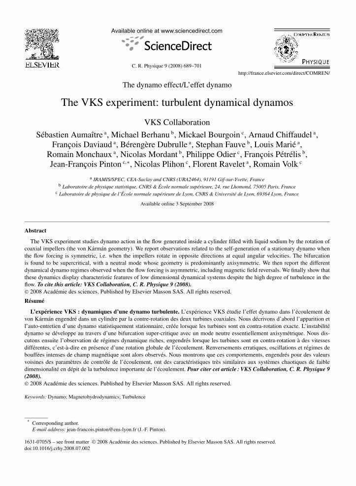
A sketch of the experiment is shown in Fig. 1. The flow is generated by rotating two disks of radius 154.5 mm,371 mm apart in a cylindrical vessel, 2R = 412 mm in inner diameter and 524 mm in length. The disks are fittedwith 8 curved blades of height h = 41.2 mm. These impellers are driven at rotation frequencies (F1,F2) up to 26 Hzby 300 kW available motor power. An oil circulation in the outer copper cylinder maintains a regulated temperaturein the range 110–160 ◦C. The mean flow has the following characteristics: the fluid is ejected radially outward bythe disks; this drives an axial flow toward the disks along their axis and a recirculation in the opposite direction

Fig. 1. Experimental setup. Note the curved impellers, the inner cylinder which separates the flow volume from the blanket of surrounding sodiumand the thin annulus in the mid plane. Also shown are the holes through which the 3D Hall probes are inserted into the vessel for magneticmeasurements. Location in (r/R, θ, x/R) coordinates of available measurement points: P1(1,π/2,0); P2(1,π/2,0.58); P3(0.25,π/2,−0.58);P4(0.25,π/2,0.58); P5(1,π,0) (see Table 1 for details concerning available measurements in different experimental runs). When referring to thecoordinates of magnetic field vector �B measured in the experiment at these different points, we will use either the Cartesian projection (Bx,By,Bz)

on the frame (�x, �y, �z) or the cylindrical projection (Br ,Bθ ,Bx) on the frame (r, θ, x). (Bθ = −By and Br = Bz for measurements at points P 1,P 2 and P 3.)

VKS Collaboration / C. R. Physique 9 (2008) 689–701 691

Table 1Experimental configurations of the four successive runs discussed here. VKS2g (September 2006) is the first run with dynamo action. Labels MPor G indicate whether a 3D probe array of Hall sensors or a single 3D gaussmeter was used. P# (cf. Fig. 1) is the location of the measurement – theinner-most sensor for the probe array

Runs Impellers Dynamo P 1 P 2 P 3 P 4 P 5

VKS2f stainless steel No MP – – – –VKS2g iron Yes MP G – – –VKS2h iron Yes G – – – MPVKS2i iron Yes – – MP G –

along the cylinder lateral boundary. In addition, in the case of counter-rotating disks studied here, the presence of astrong axial shear of azimuthal velocity in the mid-plane between the impellers generates a high level of turbulentfluctuations [15,16]. The kinetic Reynolds number is Re = KR2Fi/ν, where ν is the kinematic viscosity and K = 0.6is a coefficient that measures the efficiency of the impellers [16]. Re can be increased up to 5 × 106: the correspondingmagnetic Reynolds number is Rm = Kμ0σR2Fi ≈ 49 (at 120 ◦C), where μ0 is the magnetic permeability of vacuumand σ is the electrical conductivity of sodium.

Compared to previous VKS experiments, three modifications have been performed regarding flow generation andboundary conditions. A first modification consists of surrounding the flow by sodium at rest in another concentriccylindrical vessel, 578 mm in inner diameter. This has been shown to decrease the dynamo threshold in kinematiccomputations based on the mean flow velocity [16]. The total volume of liquid sodium is 150 l. A second geometricalmodification consists of attaching an annulus of inner radius 175 mm and thickness 5 mm along the inner cylinder inthe mid-plane between the disks. Water experiments have shown that its effect on the mean flow is to make the shearlayer sharper around the mid-plane. In addition, it reduces low frequency turbulent fluctuations, but the rms velocityfluctuations are almost unchanged (of order 40–50%) [17]. Finally, the impellers driving the flow are made of softiron. Using boundary conditions with a high permeability in order to change the dynamo threshold has been alreadyproposed [18]. It has been also shown that in the case of a Ponomarenko or G.O. Roberts flows, the addition of anexternal wall of high permeability can decrease the dynamo threshold [19]. Kinematic simulations of the VKS meanflow have shown that different ways of taking into account the sodium behind the disks lead to an increase of thedynamo threshold ranging from 12% to 150% [20]. Other kinematic simulations using a model flow show that thethreshold with boundaries of high magnetic permeability is lower than that obtained by replacing the sodium behindthe disks by an insultating medium [21], although the actual behavior may be more complex.

Magnetic measurements are performed using 3D Hall probes, and recorded with a National Instruments PXI digi-tizer. We use both a single-point (three components) Bell probe (hereafter label G-probe) connected to its associatedgaussmeter and a custom-made array where the 3D magnetic field is sampled at 10 locations along a line (hereaftercalled SM-array), every 28 mm. The array is made from Sentron 2SA-1M Hall sensors, and is air-cooled to keep thesensors temperature between 35 and 45 ◦C. For both probes, the dynamical range is 70 dB, with an AC cut-off at400 Hz for the gaussmeter and 1 kHz for the custom-made array; signals have been sampled at rates between 1 and5 kHz. The locations of the probe in each of the experimental runs discussed here are reported in Table 1.

3. Dynamo generation, symmetric forcing, F1 = F2

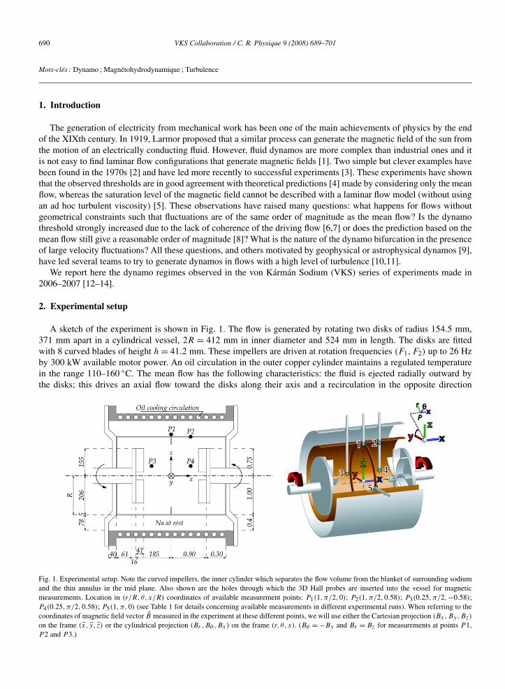
We first consider the behavior when the flow is forced by impellers counter-rotating at equal rates, F1 = F2. Fig. 2shows the time recording of the three components of �B at point P 1 when Rm is increased from 19 to 40. The largestcomponent, By , is tangent to the cylinder at the measurement location. It increases from a mean value comparableto the Earth’s magnetic field to roughly 40 G. The mean values of the other components Bx and Bz also increase(not visible on the figure because of fluctuations). Both signs of the components have been observed in different runs,depending on the sign of the residual magnetization of the disks. All components display strong fluctuations as couldbe expected in flows with Reynolds numbers larger than 106.

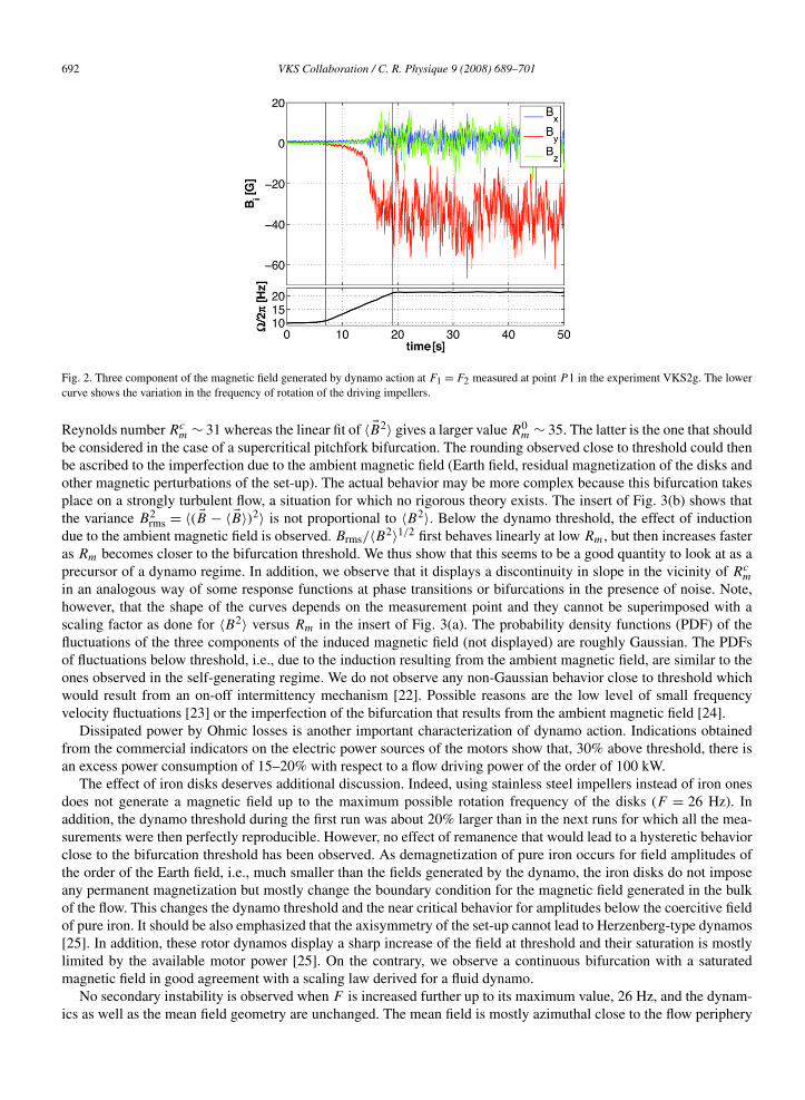
Fig. 3(a) shows the mean values of the components 〈Bi〉 of the magnetic field and Fig. 3(b) their fluctuations Bi rmsversus Rm. The fluctuations are all in the same range (3 G to 8 G, at 30% above threshold) although the correspondingmean values are very different. The time average of the square of the total magnetic field, 〈 �B2〉, is displayed in theinsert of Fig. 3(a). No hysteresis is observed. Linear fits of 〈By〉 or Bi rms displayed in Fig. 3 define a critical magnetic


Fig. 2. Three component of the magnetic field generated by dynamo action at F1 = F2 measured at point P 1 in the experiment VKS2g. The lowercurve shows the variation in the frequency of rotation of the driving impellers.

Reynolds number Rcm ∼ 31 whereas the linear fit of 〈 �B2〉 gives a larger value R0

m ∼ 35. The latter is the one that shouldbe considered in the case of a supercritical pitchfork bifurcation. The rounding observed close to threshold could thenbe ascribed to the imperfection due to the ambient magnetic field (Earth field, residual magnetization of the disks andother magnetic perturbations of the set-up). The actual behavior may be more complex because this bifurcation takesplace on a strongly turbulent flow, a situation for which no rigorous theory exists. The insert of Fig. 3(b) shows thatthe variance B2

rms = 〈( �B − 〈 �B〉)2〉 is not proportional to 〈B2〉. Below the dynamo threshold, the effect of inductiondue to the ambient magnetic field is observed. Brms/〈B2〉1/2 first behaves linearly at low Rm, but then increases fasteras Rm becomes closer to the bifurcation threshold. We thus show that this seems to be a good quantity to look at as aprecursor of a dynamo regime. In addition, we observe that it displays a discontinuity in slope in the vicinity of Rc

m

in an analogous way of some response functions at phase transitions or bifurcations in the presence of noise. Note,however, that the shape of the curves depends on the measurement point and they cannot be superimposed with ascaling factor as done for 〈B2〉 versus Rm in the insert of Fig. 3(a). The probability density functions (PDF) of thefluctuations of the three components of the induced magnetic field (not displayed) are roughly Gaussian. The PDFsof fluctuations below threshold, i.e., due to the induction resulting from the ambient magnetic field, are similar to theones observed in the self-generating regime. We do not observe any non-Gaussian behavior close to threshold whichwould result from an on-off intermittency mechanism [22]. Possible reasons are the low level of small frequencyvelocity fluctuations [23] or the imperfection of the bifurcation that results from the ambient magnetic field [24].

Dissipated power by Ohmic losses is another important characterization of dynamo action. Indications obtainedfrom the commercial indicators on the electric power sources of the motors show that, 30% above threshold, there isan excess power consumption of 15–20% with respect to a flow driving power of the order of 100 kW.

The effect of iron disks deserves additional discussion. Indeed, using stainless steel impellers instead of iron onesdoes not generate a magnetic field up to the maximum possible rotation frequency of the disks (F = 26 Hz). Inaddition, the dynamo threshold during the first run was about 20% larger than in the next runs for which all the mea-surements were then perfectly reproducible. However, no effect of remanence that would lead to a hysteretic behaviorclose to the bifurcation threshold has been observed. As demagnetization of pure iron occurs for field amplitudes ofthe order of the Earth field, i.e., much smaller than the fields generated by the dynamo, the iron disks do not imposeany permanent magnetization but mostly change the boundary condition for the magnetic field generated in the bulkof the flow. This changes the dynamo threshold and the near critical behavior for amplitudes below the coercitive fieldof pure iron. It should be also emphasized that the axisymmetry of the set-up cannot lead to Herzenberg-type dynamos[25]. In addition, these rotor dynamos display a sharp increase of the field at threshold and their saturation is mostlylimited by the available motor power [25]. On the contrary, we observe a continuous bifurcation with a saturatedmagnetic field in good agreement with a scaling law derived for a fluid dynamo.

No secondary instability is observed when F is increased further up to its maximum value, 26 Hz, and the dynam-ics as well as the mean field geometry are unchanged. The mean field is mostly azimuthal close to the flow periphery


(a)

(b)

Fig. 3. (a) Mean values of the three components of the magnetic field recorded at P 1 versus Rm (T = 120 ◦C): (Q) −〈Bx 〉, (2) −〈By 〉, (") 〈Bz〉.The inset shows the time average of the square of the total magnetic field as a function of Rm , measured at P 1 ("), or at P 2 (✩) after beingdivided by 1.8. (b) Standard deviation of the fluctuations of each components of the magnetic field recorded at P 1 versus Rm . The inset showsBrms/〈B2〉1/2. Measurements done at P 1: (Q) T = 120 ◦C, frequency increased up to 22 Hz; Measurements done at P 2: (✩) T = 120 ◦C,frequency decreased from 22 to 16.5 Hz, (1) T = 156 ◦C, frequency increased up to 22 Hz, (!) Ω/2π = 16.5 Hz, T varied from 154 to 116 ◦C,(E) Ω/2π = 22 Hz, T varied from 119 to 156 ◦C. The vertical line corresponds to Rm = 32.

whereas the azimuthal and axial components are of the same order of magnitude in the bulk of the flow. The radialcomponent is much weaker. These observations show that the mean magnetic field differs from that computed numer-ically by taking into account the mean flow alone. It was found to be an equatorial dipole [16,26,27], thus leadingto a strong radial component in the mid-plane between the impellers. A simple model of an α − ω dynamo has beenproposed to understand the experimentally observed axial dipole [28,29]: it takes into account the helical nature ofthe velocity corresponding to the flow ejected by the centrifugal force close to each impeller between the blades. Thisgives an α-effect localized close to the disks that transforms an azimuthal field into a poloidal one, whereas differen-tial rotation converts also very efficiently the poloidal component into toroidal by ω effect. However, the distributionof helicity in three-dimensional turbulence remains a challenging question. Induction measurements in [30,31] showanother possible contribution to the alpha effect, from spatial inhomogeneities in the turbulence intensity. As cal-culated in [32], there is a contribution to the mean-field alpha tensor coming from the inhomogeneity of turbulentfluctuations, with a resulting electromotive force ε ∼ (g · Ω)B, where Ω is the flow vorticity and g the normalizedgradient of turbulent fluctuations, g = (∇u2)/u2. In this case again an azimuthal Bθ field generates a jθ current, and


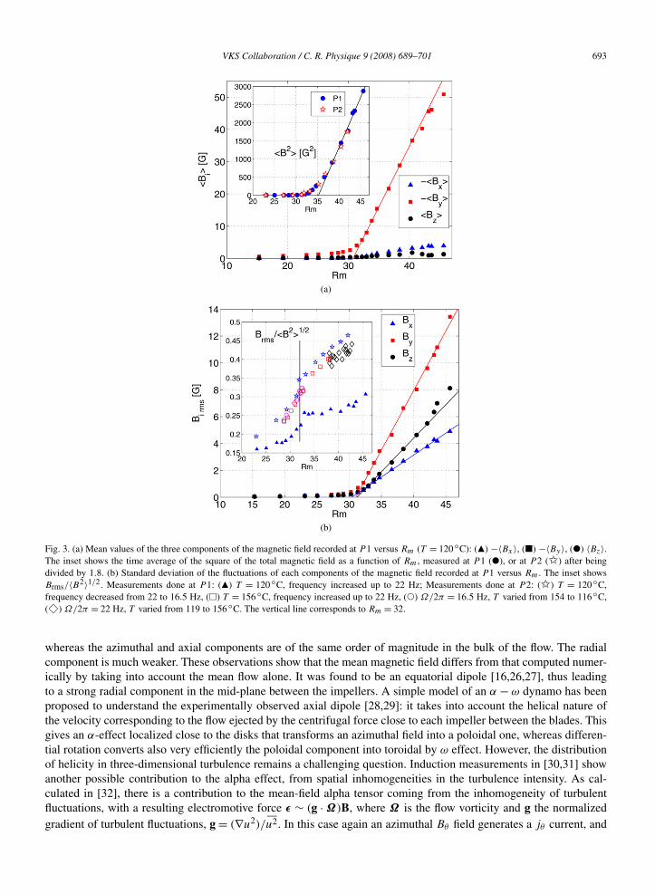
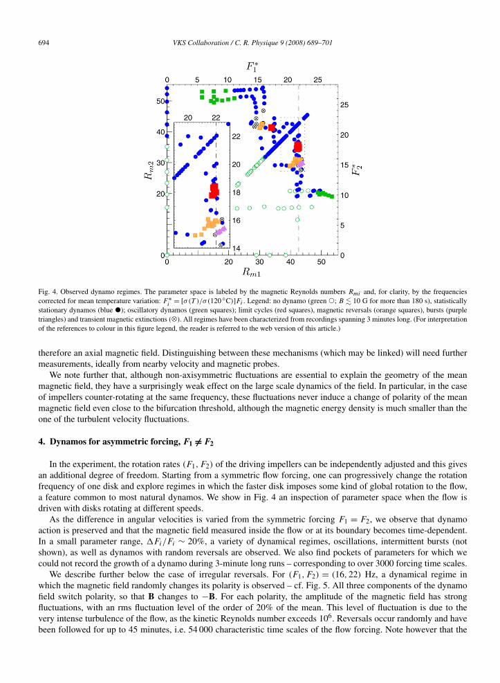
Fig. 4. Observed dynamo regimes. The parameter space is labeled by the magnetic Reynolds numbers Rmi and, for clarity, by the frequenciescorrected for mean temperature variation: F ∗

i= [σ(T )/σ(120 ◦C)]Fi . Legend: no dynamo (green !; B � 10 G for more than 180 s), statistically

stationary dynamos (blue "); oscillatory dynamos (green squares); limit cycles (red squares), magnetic reversals (orange squares), bursts (purpletriangles) and transient magnetic extinctions ('). All regimes have been characterized from recordings spanning 3 minutes long. (For interpretationof the references to colour in this figure legend, the reader is referred to the web version of this article.)

therefore an axial magnetic field. Distinguishing between these mechanisms (which may be linked) will need furthermeasurements, ideally from nearby velocity and magnetic probes.

We note further that, although non-axisymmetric fluctuations are essential to explain the geometry of the meanmagnetic field, they have a surprisingly weak effect on the large scale dynamics of the field. In particular, in the caseof impellers counter-rotating at the same frequency, these fluctuations never induce a change of polarity of the meanmagnetic field even close to the bifurcation threshold, although the magnetic energy density is much smaller than theone of the turbulent velocity fluctuations.

4. Dynamos for asymmetric forcing, F1 �= F2

In the experiment, the rotation rates (F1,F2) of the driving impellers can be independently adjusted and this givesan additional degree of freedom. Starting from a symmetric flow forcing, one can progressively change the rotationfrequency of one disk and explore regimes in which the faster disk imposes some kind of global rotation to the flow,a feature common to most natural dynamos. We show in Fig. 4 an inspection of parameter space when the flow isdriven with disks rotating at different speeds.

As the difference in angular velocities is varied from the symmetric forcing F1 = F2, we observe that dynamoaction is preserved and that the magnetic field measured inside the flow or at its boundary becomes time-dependent.In a small parameter range, Fi/Fi ∼ 20%, a variety of dynamical regimes, oscillations, intermittent bursts (notshown), as well as dynamos with random reversals are observed. We also find pockets of parameters for which wecould not record the growth of a dynamo during 3-minute long runs – corresponding to over 3000 forcing time scales.

We describe further below the case of irregular reversals. For (F1,F2) = (16,22) Hz, a dynamical regime inwhich the magnetic field randomly changes its polarity is observed – cf. Fig. 5. All three components of the dynamofield switch polarity, so that B changes to −B. For each polarity, the amplitude of the magnetic field has strongfluctuations, with an rms fluctuation level of the order of 20% of the mean. This level of fluctuation is due to thevery intense turbulence of the flow, as the kinetic Reynolds number exceeds 106. Reversals occur randomly and havebeen followed for up to 45 minutes, i.e. 54 000 characteristic time scales of the flow forcing. Note however that the


Fig. 5. Direct time recordings of the three components of the magnetic field. Disk rotation frequencies, F1 = 16 Hz, F2 = 22 Hz: Bx (blue),By (red), Bz (green). Measurement at point P1 in VKS2g. The upper graph shows the sequences of polarities for the longest run in this regime (theshaded area corresponding to the lower plot). (For interpretation of the references to colour in this figure legend, the reader is referred to the webversion of this article.)

amplitude of the magnetic field, much larger than the Earth field, is the same for both polarities. Standard deviationsare of the same order of magnitude as the mean values, although better statistics may be needed to fully convergethese estimates. The mean duration of each reversal, τ ∼ 5 s, is longer than magnetohydrodynamics time scales: theflow integral time scale is of the order of the inverse of the rotation frequencies, i.e. 0.05 s, and the ohmic diffusivetime scale is roughly τη ∼ 0.4 s. In the regime reported in Fig. 5, the polarities do not have the same probability ofobservation. Phases with a positive polarity for the largest magnetic field component have on average longer duration(〈T+〉 = 120 s) than phases with the opposite polarity (〈T−〉 = 50 s).

Concerning the dynamics of field reversals, a natural question is related to the connection between B and −B intime. The equations of magnetohydrodynamics are symmetric under the B → −B transformation so that the selectionof a polarity is a broken symmetry at the dynamo bifurcation threshold. The sequences of opposite polarities displayedin Fig. 5 act as magnetic domains along the time axis, with Ising-type walls in-between them: the magnetic fieldvanishes during the polarity change rather than rotating as in a Bloch-type wall. For other parameter values Rmi

(i = 1,2), we have also found reversals of Bloch-type. One important observation for the reversals reported here isthe correlation with the global energy budget of the flow. The total power P(t) delivered by the motors driving theflow fluctuates in time in a strongly asymmetric manner: the record shows short periods when P is much smaller thanits average. They always coincide with large variations in the magnetic field, as shown in Fig. 5. Either a reversaloccurs, or the magnetic field first decays and then grows again with its direction unchanged. Similar sequences, calledexcursions, are observed in recordings of the Earth’s magnetic field. The variation of power consumption during theweakening of the magnetic field is in agreement with the power required to sustain a steady dynamo in the VKS2experiment (drops by over 20%, that is 20 kW out of 90 kW). However, we note that in other regions of the parameterspace, different regimes also involve changes in polarity without noticeable modification of power.

We have also observed that the trajectories connecting the symmetric states B and −B are quite robust despite thestrong turbulent fluctuations of the flow. This is displayed in Fig. 6: the time evolution of reversals from up to downstates can be neatly superimposed by shifting the origin of time such that B(t = 0) = 0 for each reversal. Despite theasymmetry due to the Earth’s magnetic field, down-up reversals can be superimposed in a similar way on up-downones if −B is plotted instead of B . For each reversal the amplitude of the field first decays exponentially. A decay rate


Fig. 6. Superimposition of 6 successive reversals from up to down polarity together with 6 successive reversals from down to up polarity with thetransformation B → −B. For each of them the origin of time has been shifted such that it corresponds to B = 0. The thick black line is the averageof all reversals.

of roughly 0.8 s−1 is obtained with a log-lin plot (not shown). After changing polarity, the field amplitude increaseslinearly and then displays an overshoot before reaching its statistically stationary regime.

Further investigation of this regime will help address from an experimental perspective persistent questions aboutmagnetic field reversals. Some of these concern the role of hydrodynamics and electromagnetic boundary conditions– both of them can be experimentally adjusted. Others are related to the dynamics of the magnetic reversals. Frominspection of paleomagnetic data, it has been proposed that reversing dynamos and non-reversing ones are metastablestates in close proximity [33]. In geodynamo simulations (convective dynamos in rapidly rotating spheres), the flowis often laminar and reversals have been associated to interactions between dipole and higher order modes, with thepossibility of reversal precursor events [34]. Field reversals have also been observed in turbulence driven numericalα2 and α − ω dynamos based on mean-field magnetohydrodynamics [35,42]. In these, the role of noise was foundto be essential, together with the proximity of steady and oscillating states. In many cases, the existence of severaldynamo regimes in a narrow region of parameter space has been considered as essential. Our experiment displays thisfeature: two different stationary dynamo modes bifurcate for F1 = F2 and respectively F1 �= F2 (see section below).Their interaction gives rise to a variety of different dynamical regimes in parameter space. This is a general featurefor bifurcations of multiple codimension.

5. Transitions and chaotic features

In the VKS experiment, depending on the amount of global rotation, both stationary regimes are observed as wellas several secondary bifurcations that lead to more complex dynamics including field reversals – see above. The aimof this section is to discuss these different regimes and to illustrate that they can be understood as the result of a fewcompeting modes in the vicinity of the dynamo threshold.

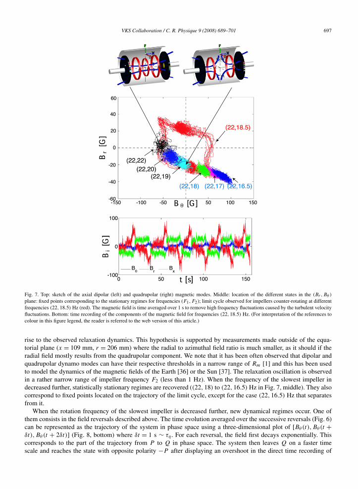
Let us consider the case where we start from impellers rotating at 22 Hz, and then the frequency of an impeller,say F2, is decreased, F1 being kept constant. We first observe a statistically stationary dynamo regime with a dominantazimuthal mean field close to the flow periphery (Fig. 7, top left). This corresponds to the trace labeled (22,22) inthe (Br,Bθ ) plane of Fig. 7 (middle). As the frequency of the slower impeller is decreased, we obtain other stationarydynamo regimes for which the radial component of the mean field increases and then becomes larger than the az-imuthal one ((22,20) and (22,19)). When we tune the impeller frequencies to 22 and 18.5 Hz respectively, a globalbifurcation to a limit cycle occurs. We observe that the trajectory of this limit cycle goes through the location of theprevious fixed points related to the stationary regimes. This transition thus looks like the one of an excitable system:an elementary example of this type of bifurcation is provided by a simple pendulum submitted to a constant torque.As the value of the torque is increased, the stable equilibrium of the pendulum becomes more and more tilted from thevertical and for a critical torque corresponding to the angle π/2, the pendulum undergoes a saddle-node bifurcationto a limit cycle that goes through the previous fixed points. Direct time-recordings of the magnetic field, measured atthe periphery of the flow in the mid-plane between the two impellers, are displayed in Fig. 7 (bottom). We propose toascribe the strong radial component (in green) that switches between ±25 G to a quadrupolar mode (see Fig. 7, topright). Its interaction with the dipolar mode (Fig. 7, top left) that is the dominant one for exact counter-rotation, gives


Fig. 7. Top: sketch of the axial dipolar (left) and quadrupolar (right) magnetic modes. Middle: location of the different states in the (Br ,Bθ )

plane: fixed points corresponding to the stationary regimes for frequencies (F1,F2); limit cycle observed for impellers counter-rotating at differentfrequencies (22,18.5) Hz (red). The magnetic field is time averaged over 1 s to remove high frequency fluctuations caused by the turbulent velocityfluctuations. Bottom: time recording of the components of the magnetic field for frequencies (22,18.5) Hz. (For interpretation of the references tocolour in this figure legend, the reader is referred to the web version of this article.)

rise to the observed relaxation dynamics. This hypothesis is supported by measurements made outside of the equa-torial plane (x = 109 mm, r = 206 mm) where the radial to azimuthal field ratio is much smaller, as it should if theradial field mostly results from the quadrupolar component. We note that it has been often observed that dipolar andquadrupolar dynamo modes can have their respective thresholds in a narrow range of Rm [1] and this has been usedto model the dynamics of the magnetic fields of the Earth [36] or the Sun [37]. The relaxation oscillation is observedin a rather narrow range of impeller frequency F2 (less than 1 Hz). When the frequency of the slowest impeller indecreased further, statistically stationary regimes are recovered ((22,18) to (22,16.5) Hz in Fig. 7, middle). They alsocorrespond to fixed points located on the trajectory of the limit cycle, except for the case (22,16.5) Hz that separatesfrom it.

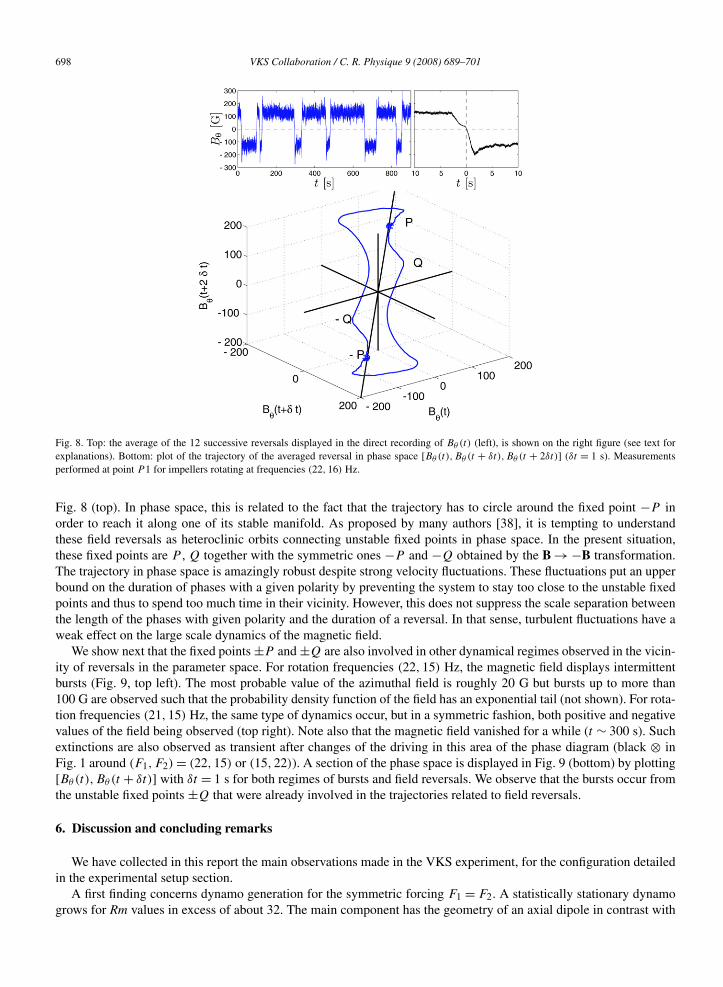
When the rotation frequency of the slowest impeller is decreased further, new dynamical regimes occur. One ofthem consists in the field reversals described above. The time evolution averaged over the successive reversals (Fig. 6)can be represented as the trajectory of the system in phase space using a three-dimensional plot of [Bθ(t),Bθ (t +δt),Bθ (t + 2δt)] (Fig. 8, bottom) where δt = 1 s ∼ τη. For each reversal, the field first decays exponentially. Thiscorresponds to the part of the trajectory from P to Q in phase space. The system then leaves Q on a faster timescale and reaches the state with opposite polarity −P after displaying an overshoot in the direct time recording of


Fig. 8. Top: the average of the 12 successive reversals displayed in the direct recording of Bθ (t) (left), is shown on the right figure (see text forexplanations). Bottom: plot of the trajectory of the averaged reversal in phase space [Bθ (t),Bθ (t + δt),Bθ (t + 2δt)] (δt = 1 s). Measurementsperformed at point P 1 for impellers rotating at frequencies (22,16) Hz.

Fig. 8 (top). In phase space, this is related to the fact that the trajectory has to circle around the fixed point −P inorder to reach it along one of its stable manifold. As proposed by many authors [38], it is tempting to understandthese field reversals as heteroclinic orbits connecting unstable fixed points in phase space. In the present situation,these fixed points are P , Q together with the symmetric ones −P and −Q obtained by the B → −B transformation.The trajectory in phase space is amazingly robust despite strong velocity fluctuations. These fluctuations put an upperbound on the duration of phases with a given polarity by preventing the system to stay too close to the unstable fixedpoints and thus to spend too much time in their vicinity. However, this does not suppress the scale separation betweenthe length of the phases with given polarity and the duration of a reversal. In that sense, turbulent fluctuations have aweak effect on the large scale dynamics of the magnetic field.

We show next that the fixed points ±P and ±Q are also involved in other dynamical regimes observed in the vicin-ity of reversals in the parameter space. For rotation frequencies (22,15) Hz, the magnetic field displays intermittentbursts (Fig. 9, top left). The most probable value of the azimuthal field is roughly 20 G but bursts up to more than100 G are observed such that the probability density function of the field has an exponential tail (not shown). For rota-tion frequencies (21,15) Hz, the same type of dynamics occur, but in a symmetric fashion, both positive and negativevalues of the field being observed (top right). Note also that the magnetic field vanished for a while (t ∼ 300 s). Suchextinctions are also observed as transient after changes of the driving in this area of the phase diagram (black ⊗ inFig. 1 around (F1,F2) = (22,15) or (15,22)). A section of the phase space is displayed in Fig. 9 (bottom) by plotting[Bθ(t),Bθ (t + δt)] with δt = 1 s for both regimes of bursts and field reversals. We observe that the bursts occur fromthe unstable fixed points ±Q that were already involved in the trajectories related to field reversals.

6. Discussion and concluding remarks

We have collected in this report the main observations made in the VKS experiment, for the configuration detailedin the experimental setup section.

A first finding concerns dynamo generation for the symmetric forcing F1 = F2. A statistically stationary dynamogrows for Rm values in excess of about 32. The main component has the geometry of an axial dipole in contrast with


Fig. 9. Top: time recordings of the azimuthal component of the magnetic field observed for impellers rotating at (22,15) Hz (left), (21,15) Hz(right). Bottom: plot of a cut in phase space [Bθ (t),Bθ (t + δt)] with δt = 1 s for three regimes: in black for field reversals reported in Fig. 3,the magnetic field being rescaled by an ad-hoc factor accounting that the probe location is not in the mid-plane. In blue, for symmetric bursts(21,15) Hz and in red for asymmetric bursts (22,15) Hz. In these last two plots the magnetic field is time averaged over 0.25 s to remove highfrequency fluctuations.

kinematic dynamo codes taking into account only the mean flow. Cowling’s theorem shows that non-axisymmetricturbulent fluctuations are essential for the generation of this dynamo. In addition the threshold value is also lower thanthe kinematic predictions using the mean flow, that are in the range Rc

m = 40 to 150 depending on different boundaryconditions on the disks and on configurations of the flow behind them [16,20]. The generation of the statisticallystationary dynamo driven at F1 = F2 share many characteristic with bifurcations in the presence of noise. For instancethreshold values defined using mean field or rms quantities differ. As shown in much simpler experiments, differentchoices of an order parameter (mean value of the amplitude of the unstable mode or its higher moments, its mostprobable value, etc.) can lead to qualitatively different bifurcation diagrams [39]. This illustrates the ambiguity in thedefinition of the order parameter for bifurcations in the presence of fluctuations or noise. In the present experiment,fluctuations enter both multiplicatively, because of the turbulent velocity, and additively, due to the interaction of thevelocity field with the ambient magnetic field.

A second noteworthy feature is that different dynamical regimes are generated when the flow is driven with im-pellers counter-rotating at different rates. In addition, these regimes display several characteristic of low dimensionaldynamical systems: global bifurcations from fixed points to a relaxation cycle, heteroclinic orbits, chaotic bursts fromunstable fixed points. These dynamics can be understood as the ones resulting from the competition between a fewnearly critical modes. This has been observed in other hydrodynamical instabilities since the early experimental studieson codimension-two bifurcations [40]. Competing critical modes have been already considered as phenomenological


models of the dynamics of the magnetic fields of the Earth [36,38] or the Sun [41,37] and similar type of dynam-ics have been obtained. It has been also observed in simulations [34] or mean field models [42] that magnetic fieldreversals can occur when a stationary and an oscillatory modes are in proximity and a simple analytic model hasbeen designed in this spirit [43]. It is also well known since Rikitake that dynamo models corresponding to a drastictruncation of the governing equations can give rise to complex temporal dynamics [44]. We emphasize that what isremarkable in the present study is the robustness of these low dimensional dynamical features that are not smearedout despite large turbulent fluctuations of the flow that generates the dynamo field. A possible explanation is that thelarge scale magnetic field is too slow to follow velocity perturbations with time scales comparable to the rotation rateof the impellers or smaller.

Acknowledgements

We thank M. Moulin, C. Gasquet, J.-B. Luciani, A. Skiara, D. Courtiade, J.-F. Point, P. Metz and V. Padilla for theirtechnical assistance. This work is supported by ANR05-0268-03, Direction des Sciences de la Matière et Directionde l’Énergie Nucléaire of CEA, Ministère de la Recherche and CNRS. The experiment is operated at CEA/CadaracheDEN/DTN.

References

[1] H.K. Moffatt, Magnetic Field Generation in Electrically Conducting Fluids, Cambridge University Press, Cambridge, 1978.[2] G.O. Roberts, Philos. Trans. Roy. Soc. London A 271 (1972) 411–454;

Yu.B. Ponomarenko, J. Appl. Mech. Tech. Phys. 14 (1973) 775–778.[3] R. Stieglitz, U. Müller, Phys. Fluids 13 (2001) 561;

A. Gailitis, et al., Phys. Rev. Lett. 86 (2001) 3024.[4] F.H. Busse, U. Müller, R. Stieglitz, A. Tilgner, Magnetohydrodynamics 32 (1996) 235–248;

K.-H. Rädler, E. Apstein, M. Rheinhardt, M. Schüler, Studia Geophys. Geod. 42 (1998) 224–231;A. Gailitis, et al., Magnetohydrodynamics 38 (2002) 5–14.

[5] F. Pétrélis, S. Fauve, Eur. Phys. J. B 22 (2001) 273–276.[6] A.A. Schekochihin, et al., Phys. Rev. Lett. 92 (2004) 054502;

S. Boldyrev, F. Cattaneo, Phys. Rev. Lett. 92 (2004) 144501 and references therein.[7] J.-P. Laval, et al., Phys. Rev. Lett. 96 (2006) 204503.[8] Y. Ponty, et al., Phys. Rev. Lett. 94 (2005) 164502;

Y. Ponty, et al., New. J. Phys. 9 (2007) 296.[9] H.C. Nataf, et al., GAFD 100 (2006) 281.

[10] P. Odier, J.F. Pinton, S. Fauve, Phys. Rev. E 58 (1998) 7397–7401;N.L. Peffley, A.B. Cawthorne, D.P. Lathrop, Phys. Rev. E 61 (2000) 5287–5294;E.J. Spence, et al., Phys. Rev. Lett. 96 (2006) 055002;R. Stepanov, et al., Phys. Rev. E 73 (2006) 046310.

[11] M. Bourgoin, et al., Phys. Fluids 14 (2002) 3046;F. Pétrélis, et al., Phys. Rev. Lett. 90 (17) (2003) 174501;R. Volk, et al., Phys. Rev. Lett. 97 (2006) 074501.

[12] R. Monchaux, et al., Phys. Rev. Lett. 98 (2007) 044502.[13] M. Berhanu, et al., Europhys. Lett. 77 (2007) 59001.[14] F. Ravelet, et al., Chaotic dynamos generated by a turbulent flow of liquid sodium, Phys. Rev. Lett. 101 (2008) 074502.[15] L. Marié, F. Daviaud, Phys. Fluids 16 (2004) 457.[16] F. Ravelet, et al., Phys. Fluids 17 (2005) 117104.[17] F. Ravelet, PhD Thesis, Ecole Polytechnique, 2005, http://tel.archives-ouvertes.fr/tel-00011016/en/.[18] S. Fauve, F. Pétrélis, The dynamo effect, in: J.-A. Sepulchre (Ed.), Peyresq Lectures on Nonlinear Phenomena, vol. II, World Scientific, 2003,

pp. 1–64.[19] R. Avalos-Zuniga, F. Plunian, A. Gailitis, Phys. Rev. E 68 (2003) 066307.[20] F. Stefani, et al., Eur. J. Mech. B 25 (2006) 894.[21] C. Gissinger, et al., Europhys. Lett. 82 (2008) 29001.[22] D. Sweet, et al., Phys. Rev. E 63 (2001) 066211.[23] S. Aumaître, F. Pétrélis, K. Mallick, Phys. Rev. Lett. 95 (2005) 064101.[24] F. Pétrélis, S. Aumaître, Eur. Phys. J. B 51 (2006) 357.[25] F.J. Lowes, I. Wilkinson, Nature 198 (1963) 1158;

F.J. Lowes, I. Wilkinson, Nature 219 (1968) 717.[26] L. Marié, et al., Eur. Phys. J. B 33 (2003) 469.[27] M. Bourgoin, et al., Phys. Fluids 16 (2004) 2529.


[28] F. Pétrélis, N. Mordant, S. Fauve, GAFD 101 (2007) 289.[29] R. Laguerre, C. Nore, A. Ribeiro, J. Léorat, J.-L. Guermond, F. Plunian, Impact of turbines in the VKS2 dynamo experiment, arXiv: 0805.2805.[30] R. Stepanov, et al., Phys. Rev. E 73 (2006) 046310.[31] R. Volk, PhD thesis, Ecole Normale Supérieure de Lyon, 2005, http://tel.archives-ouvertes.fr/tel-00011221/en/.[32] K.-H. Rädler, R. Stepanov, Phys. Rev. E 73 (2006) 056311.[33] P.L. MacFadden, R.T. Merrill, Phys. Earth Planet. Inter. 91 (1995) 253.[34] G.R. Sarson, C.A. Jones, Phys. Earth Planet. Inter. 111 (1999) 3;

J. Wicht, P. Olson, Geochem. Geophys. Geosys. (G-cubed) 5 (2004).[35] A. Giesecke, G.R. Rüdiger, D. Elstner, Astron. Nachr. 326 (2005) 693;

L. Widrow, Rev. Mod. Phys. 74 (2002) 775.[36] I. Melbourne, M.R.E. Proctor, A.M. Rucklidge, Dynamo and dynamics, a mathematical challenge, in: P. Chossat, et al. (Eds.), Kluwer Aca-

demic Publishers, 2001, pp. 363–370.[37] E. Knobloch, A.S. Landsberg, Mon. Not. R. Astron. Soc. 278 (1996) 294.[38] P. Chossat, D. Armbruster, Proc. Roy. Soc. London A 459 (2003) 577 and references therein.[39] R. Berthet, et al., Physica D 174 (2003) 84–99.[40] S. Fauve, et al., Phys. Rev. Lett. 55 (1985) 208;

R.W. Walden, et al., Phys. Rev. Lett. 55 (1985) 496;I. Rehberg, et al., Phys. Rev. Lett. 55 (1985) 500.

[41] S.M. Tobias, N.O. Weiss, V. Kirk, Mon. Not. R. Astron. Soc. 273 (1995) 1150.[42] F. Stefani, G. Gerbeth, Phys. Rev. Lett. 94 (2005) 184506.[43] P. Hoyng, J.J. Duistermaat, Europhys. Lett. 68 (2004) 177.[44] T. Rikitake, Proc. Camb. Philos. Soc. 54 (1958) 89;

D.W. Allan, Proc. Camb. Philos. Soc. 58 (1962) 671;A.E. Cook, P.H. Roberts, Proc. Camb. Philos. Soc. 68 (1970) 547;W.V.R. Malkus, EOS, Trans. Am. Geophys. Union 53 (1972) 617;P. Nozières, Phys. Earth Planet. Inter. 17 (1978) 55.

The VKS experiment: turbulent dynamical dynamosperso.ens-lyon.fr/nicolas.plihon/VKS/Pub/Aumaitre_CRAS_9.pdfThe VKS experiment: turbulent dynamical dynamos VKS Collaboration Sébastien

Documents