The Value of Good Sampling - heathandsherwood64.comheathandsherwood64.com/pdf/The Value of Good Sampling-Presentatio… · Grade / Recovery • This statement can be found in the

The Value of Good

Sampling

1

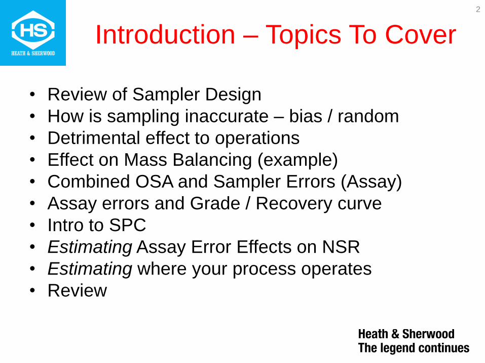
Introduction – Topics To Cover

• Review of Sampler Design

• How is sampling inaccurate – bias / random

• Detrimental effect to operations

• Effect on Mass Balancing (example)

• Combined OSA and Sampler Errors (Assay)

• Assay errors and Grade / Recovery curve

• Intro to SPC

• Estimating Assay Error Effects on NSR

• Estimating where your process operates

• Review

2

3

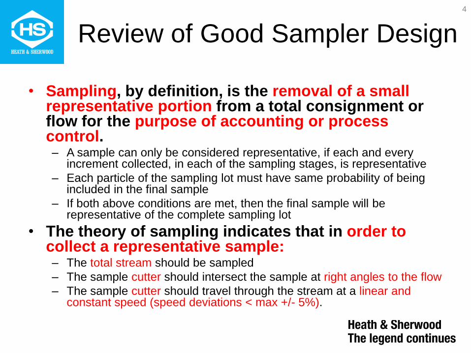
Review of Good Sampler Design

• Sampling, by definition, is the removal of a small representative portion from a total consignment or flow for the purpose of accounting or process control. – A sample can only be considered representative, if each and every

increment collected, in each of the sampling stages, is representative

– Each particle of the sampling lot must have same probability of being included in the final sample

– If both above conditions are met, then the final sample will be representative of the complete sampling lot

• The theory of sampling indicates that in order to collect a representative sample: – The total stream should be sampled

– The sample cutter should intersect the sample at right angles to the flow

– The sample cutter should travel through the stream at a linear and constant speed (speed deviations < max +/- 5%).

4

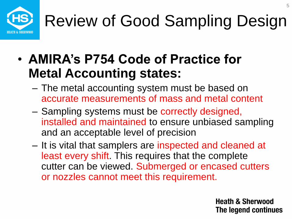
Review of Good Sampling Design

• AMIRA’s P754 Code of Practice for Metal Accounting states: – The metal accounting system must be based on

accurate measurements of mass and metal content

– Sampling systems must be correctly designed, installed and maintained to ensure unbiased sampling and an acceptable level of precision

– It is vital that samplers are inspected and cleaned at least every shift. This requires that the complete cutter can be viewed. Submerged or encased cutters or nozzles cannot meet this requirement.

5

Cutter Inspection Port

6

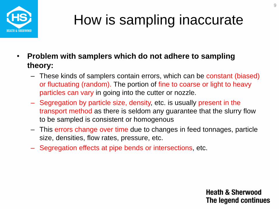
How is sampling inaccurate

• Problem with samplers which do not adhere to sampling

theory:

– These kinds of samplers contain errors, which can be constant (biased)

or fluctuating (random). The portion of fine to coarse or light to heavy

particles can vary in going into the cutter or nozzle.

– Segregation by particle size, density, etc. is usually present in the

transport method as there is seldom any guarantee that the slurry flow

to be sampled is consistent or homogenous

– This errors change over time due to changes in feed tonnages, particle

size, densities, flow rates, pressure, etc.

– Segregation effects at pipe bends or intersections, etc.

9

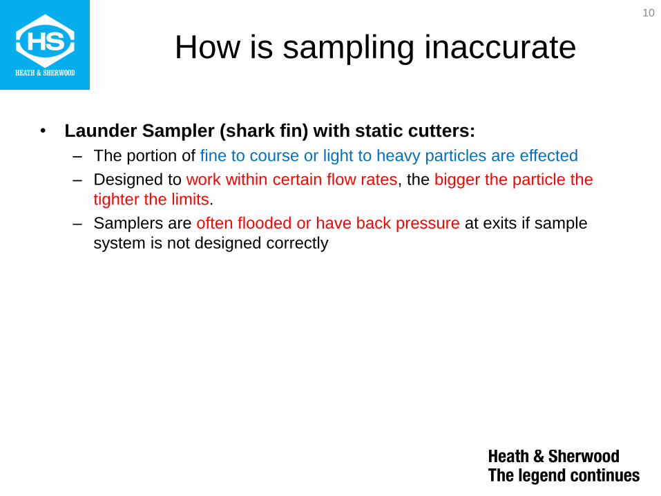
How is sampling inaccurate

• Launder Sampler (shark fin) with static cutters:

– The portion of fine to course or light to heavy particles are effected

– Designed to work within certain flow rates, the bigger the particle the

tighter the limits.

– Samplers are often flooded or have back pressure at exits if sample

system is not designed correctly

10

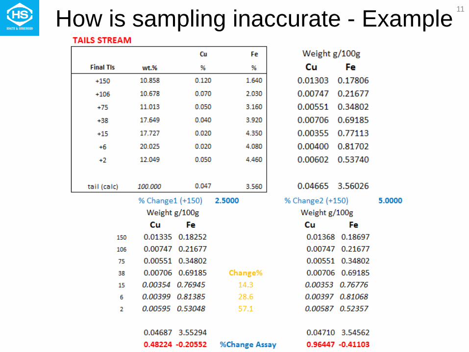
How is sampling inaccurate - Example 11

Detrimental effects to operations

• The assays from samples are used for control and accounting purposes

• Planning

– Production targets

– Plant need to make a certain amount of money to pay its bills and make

a profit. This effects how much tonnage to push through a mill.

• Plant control

– Grade / Recoveries

– Target values for these are set and accurate assays are required to

achieve this.

• Metallurgical Accounting

– Unbalanced results (poor sampling, assaying or weighing of stream)

– Unaccounted loss (lack of measurement accuracy)

12

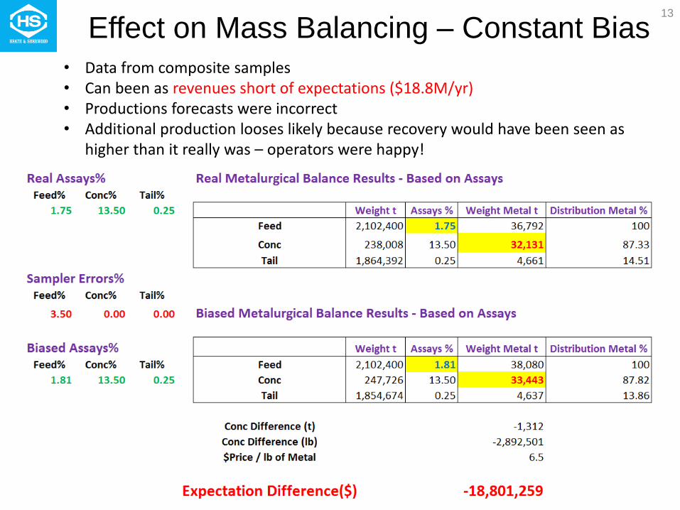
Effect on Mass Balancing – Constant Bias • Data from composite samples • Can been as revenues short of expectations ($18.8M/yr) • Productions forecasts were incorrect • Additional production looses likely because recovery would have been seen as

higher than it really was – operators were happy!

13

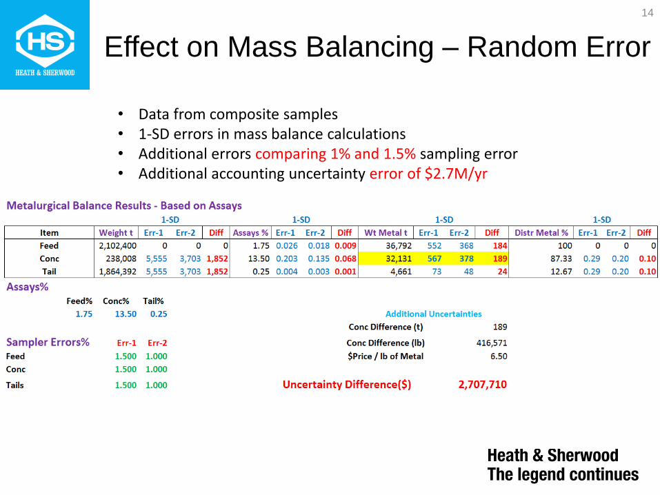
Effect on Mass Balancing – Random Error

• Data from composite samples • 1-SD errors in mass balance calculations • Additional errors comparing 1% and 1.5% sampling error • Additional accounting uncertainty error of $2.7M/yr

14

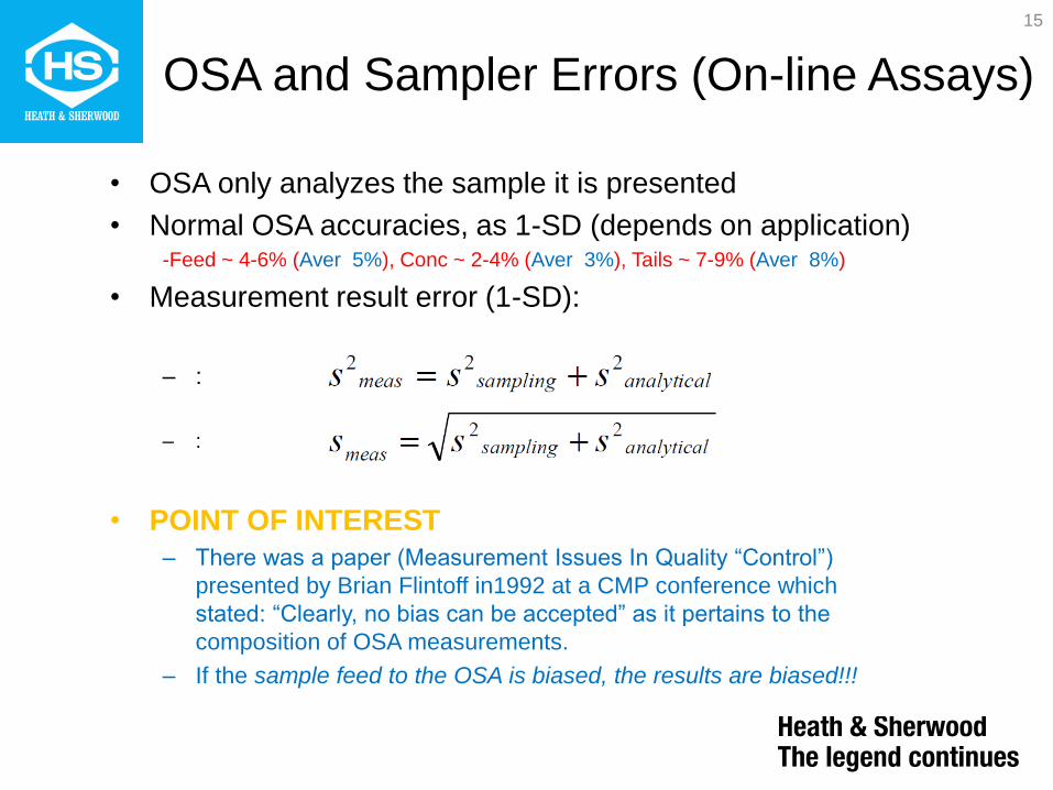
OSA and Sampler Errors (On-line Assays)

• OSA only analyzes the sample it is presented

• Normal OSA accuracies, as 1-SD (depends on application) -Feed ~ 4-6% (Aver 5%), Conc ~ 2-4% (Aver 3%), Tails ~ 7-9% (Aver 8%)

• Measurement result error (1-SD):

– :

– :

• POINT OF INTEREST

– There was a paper (Measurement Issues In Quality “Control”)

presented by Brian Flintoff in1992 at a CMP conference which

stated: “Clearly, no bias can be accepted” as it pertains to the

composition of OSA measurements.

– If the sample feed to the OSA is biased, the results are biased!!!

15

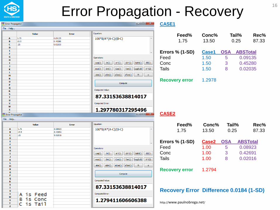
Error Propagation - Recovery CASE1

Feed% Conc% Tail% Rec%

1.75 13.50 0.25 87.33

Errors % (1-SD) Case1 OSA ABSTotal

Feed 1.50 5 0.09135

Conc 1.50 3 0.45280

Tails 1.50 8 0.02035

Recovery error 1.2978

CASE2

Feed% Conc% Tail% Rec%

1.75 13.50 0.25 87.33

Errors % (1-SD) Case2 OSA ABSTotal

Feed 1.00 5 0.08923

Conc 1.00 3 0.42691

Tails 1.00 8 0.02016

Recovery error 1.2794

Recovery Error Difference 0.0184 (1-SD)

http://www.paulnobrega.net/

16

Grade / Recovery

• This statement can be found in the Will’s Mineral Processing Technology book:

“The aim (of a flotation control system) should be to improve the metallurgical

efficiency, i.e. to produce the best possible grade-recovery curve, and to stabilize

the process at the concentrate grade which will produce the most economic return

from the throughput.”

• This statement has a few key points:

– A concentrate grade is decided upon ( could be by planer, metallurgist,

control system or other and depends on feed grade)

– Keep the process stable ( upsets are not good)

– Increase the recovery as close as possible, to the best grade-recovery

curve, without de-stabilizing (upsetting) the circuit

– Maximize recovery at a target grade

17

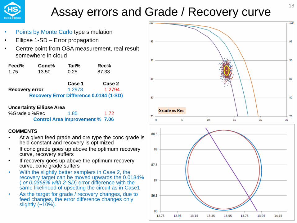
Assay errors and Grade / Recovery curve

• Points by Monte Carlo type simulation

• Ellipse 1-SD – Error propagation

• Centre point from OSA measurement, real result

somewhere in cloud

Feed% Conc% Tail% Rec%

1.75 13.50 0.25 87.33

Case 1 Case 2

Recovery error 1.2978 1.2794

Recovery Error Difference 0.0184 (1-SD)

Uncertainty Ellipse Area

%Grade x %Rec 1.85 1.72

Control Area Improvement % 7.06

COMMENTS

• At a given feed grade and ore type the conc grade is held constant and recovery is optimized

• If conc grade goes up above the optimum recovery curve, recovery suffers

• If recovery goes up above the optimum recovery curve, conc grade suffers

• With the slightly better samplers in Case 2, the recovery target can be moved upwards the 0.0184% ( or 0.0368% with 2-SD) error difference with the same likelihood of upsetting the circuit as in Case1

• As the target for grade / recovery changes, due to feed changes, the error difference changes only slightly (~10%).

18

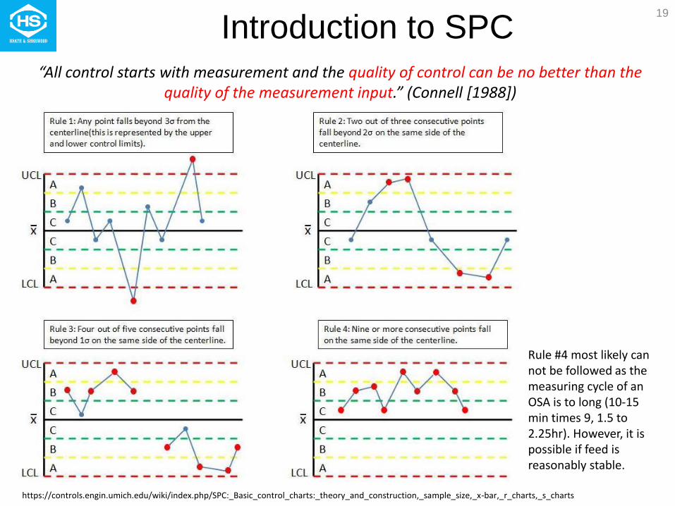
Introduction to SPC

https://controls.engin.umich.edu/wiki/index.php/SPC:_Basic_control_charts:_theory_and_construction,_sample_size,_x-bar,_r_charts,_s_charts

“All control starts with measurement and the quality of control can be no better than the quality of the measurement input.” (Connell [1988])

Rule #4 most likely can not be followed as the measuring cycle of an OSA is to long (10-15 min times 9, 1.5 to 2.25hr). However, it is possible if feed is reasonably stable.

19

Introduction to SPC

• Control limits for grade / recovery depend upon the accuracy of the analyzer / samplers • Example chart of recovery control, target shifted up 1-SD difference, 0.0184%

Probability of error

detection over 2-SD UCL is the still better than in Case #1 Probability of error detection over 1-SD UCL is the same in both cases Target moved up 1-SD difference ( 0.0184 ) Tighter control limits at 1-SD LCL and 2-SD LCL

20

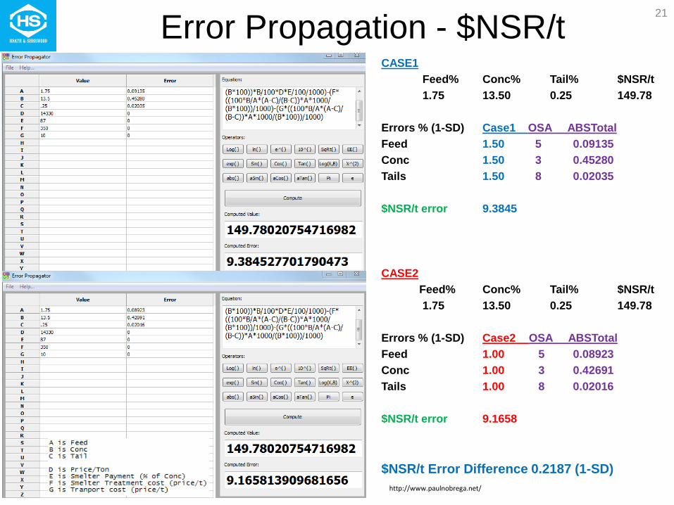
Error Propagation - $NSR/t CASE1

Feed% Conc% Tail% $NSR/t

1.75 13.50 0.25 149.78

Errors % (1-SD) Case1 OSA ABSTotal

Feed 1.50 5 0.09135

Conc 1.50 3 0.45280

Tails 1.50 8 0.02035

$NSR/t error 9.3845

CASE2

Feed% Conc% Tail% $NSR/t

1.75 13.50 0.25 149.78

Errors % (1-SD) Case2 OSA ABSTotal

Feed 1.00 5 0.08923

Conc 1.00 3 0.42691

Tails 1.00 8 0.02016

$NSR/t error 9.1658

$NSR/t Error Difference 0.2187 (1-SD)

http://www.paulnobrega.net/

21

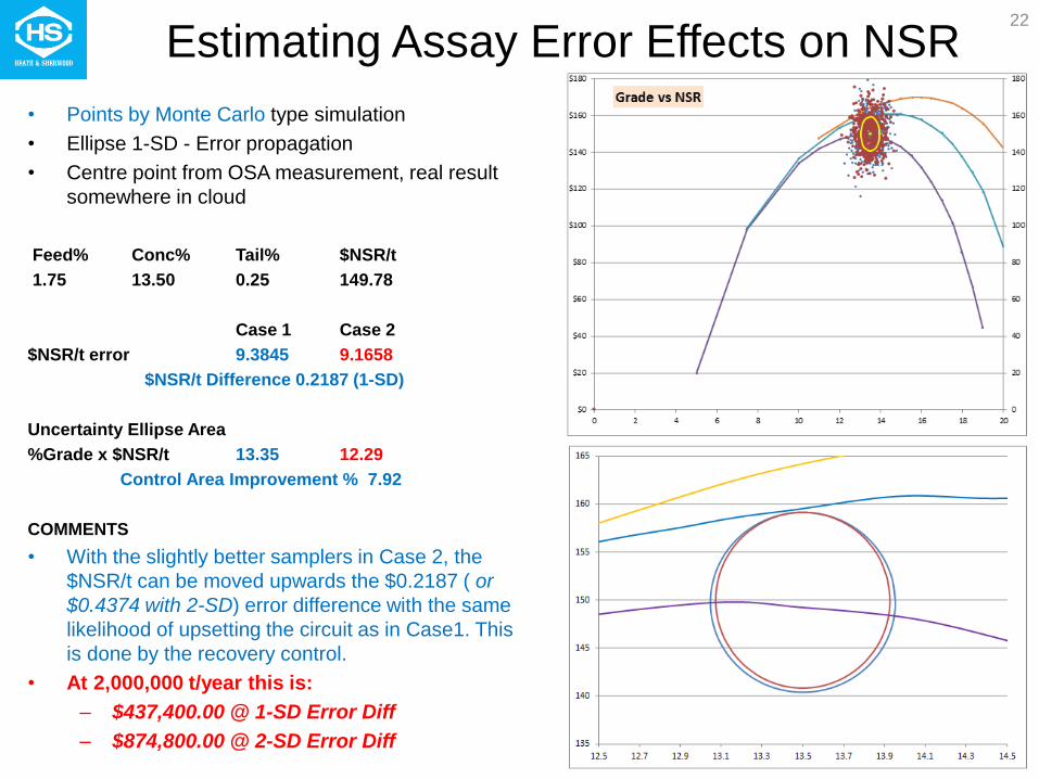
Estimating Assay Error Effects on NSR

• Points by Monte Carlo type simulation

• Ellipse 1-SD - Error propagation

• Centre point from OSA measurement, real result

somewhere in cloud

Feed% Conc% Tail% $NSR/t

1.75 13.50 0.25 149.78

Case 1 Case 2

$NSR/t error 9.3845 9.1658

$NSR/t Difference 0.2187 (1-SD)

Uncertainty Ellipse Area

%Grade x $NSR/t 13.35 12.29

Control Area Improvement % 7.92

COMMENTS

• With the slightly better samplers in Case 2, the

$NSR/t can be moved upwards the $0.2187 ( or

$0.4374 with 2-SD) error difference with the same

likelihood of upsetting the circuit as in Case1. This

is done by the recovery control.

• At 2,000,000 t/year this is:

– $437,400.00 @ 1-SD Error Diff

– $874,800.00 @ 2-SD Error Diff

22

Estimating where your process operates

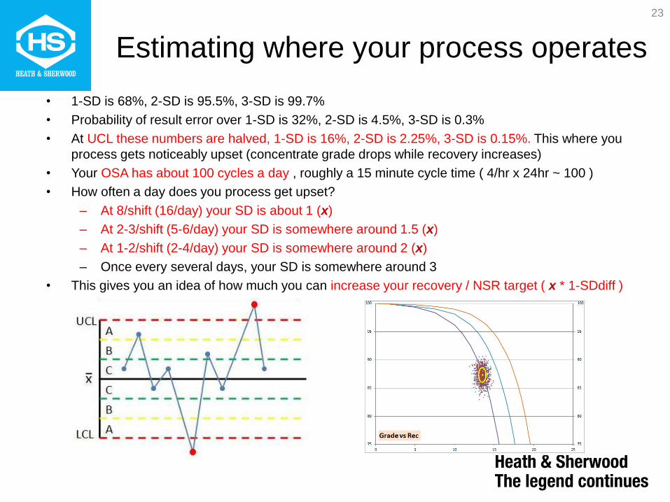
• 1-SD is 68%, 2-SD is 95.5%, 3-SD is 99.7%

• Probability of result error over 1-SD is 32%, 2-SD is 4.5%, 3-SD is 0.3%

• At UCL these numbers are halved, 1-SD is 16%, 2-SD is 2.25%, 3-SD is 0.15%. This where you

process gets noticeably upset (concentrate grade drops while recovery increases)

• Your OSA has about 100 cycles a day , roughly a 15 minute cycle time ( 4/hr x 24hr ~ 100 )

• How often a day does you process get upset?

– At 8/shift (16/day) your SD is about 1 (x)

– At 2-3/shift (5-6/day) your SD is somewhere around 1.5 (x)

– At 1-2/shift (2-4/day) your SD is somewhere around 2 (x)

– Once every several days, your SD is somewhere around 3

• This gives you an idea of how much you can increase your recovery / NSR target ( x * 1-SDdiff )

23

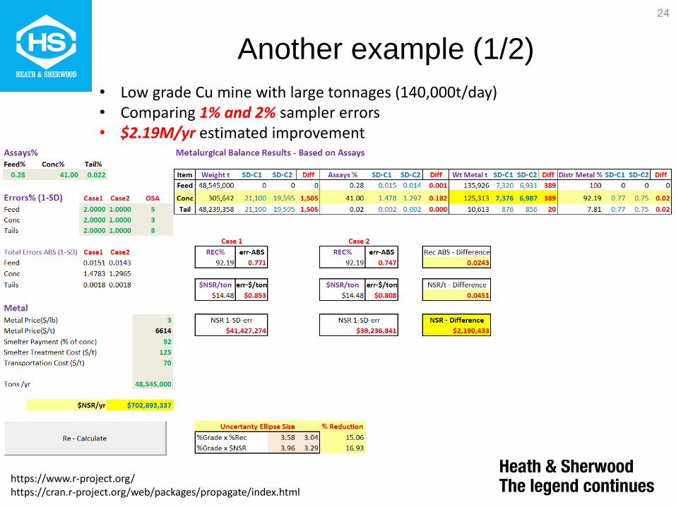
Another example (1/2)

• Low grade Cu mine with large tonnages (140,000t/day) • Comparing 1% and 2% sampler errors • $2.19M/yr estimated improvement

https://www.r-project.org/ https://cran.r-project.org/web/packages/propagate/index.html

24

Another example (2/2)

• Low grade Cu mine with large tonnages (140,000t/day) • Comparing 1% and 3% sampler errors • $5.60M/yr estimated improvement

https://www.r-project.org/ https://cran.r-project.org/web/packages/propagate/index.html

25

Review

• With smaller errors in online assays, you can get better grade / recovery control.

• With small errors improvements in online assays, you can get better $NSR/t

returns.

• With smaller errors in online assays recovery targets can get closer to the optimal

grade / recovery curve

• Good representative sampling requires cross cut samplers which sample the

complete stream

• International Sampling Standard and AMIRA Code requires good sampling

practices.

• Sampling errors can be biased or random

• Sampling errors effect production plans, your control system and metallurgical

accounting processes

“THIS IS THE VALUE OF GOOD SAMPLING“

• With tools available online “Error Propagation” can be done by anyone. You don’t

need to know how to partially differentiate (calculus).

26

Thank-you

from

HEATH & SHERWOOD

Presentation Link http://heathandsherwood64.com/products/sampling/linear_samplers

27

28