The Valuation of Derivatives on Carbon Emission Certi ...swiss.cfa/SiteCollectionDocuments/CO2_Paper_CFA_new.pdf · The Valuation of Derivatives on Carbon Emission Certi cates - a

The Valuation of Derivatives on

Carbon Emission Certificates - a

GARCH Approach

Philipp Iseneggera

Rico von Wyssb

February 2009

Abstract

The introduction of the trade of carbon emission certificates (EUA) has led tothe emergence of a variety of derivatives on this underlying. We investigatethe dynamics of the ECX December 2008 EUA futures’ returns and find ex-cess kurtosis and evidence for heteroscedasticity. The model estimation andthe subsequently performance analysis of the models, suggest a GARCH(1,1)model to appropriately reproduce the futures’ dynamics. The derivatives aresubsequently valued in a risk neutral framework using Monte Carlo simulation.

For short time horizons, the valuation outcomes are quite precise. With anincreased time period in the simulation the valuation’s accuracy is not outstand-ing, yet with respect to barrier call options and index trackers quite good resultcan be obtained. However, regarding barrier put options, there is a certainamount of mispricing in the results. The reason for this outcome is that due tothe drift in the unadjusted futures’ price simulations, disproportionately manyrealizations are knocked out.

The comparably small deviation of the valuation results from the observedmarket prices regarding the participation certificates as well as concerning thecall options provide an indication of fair pricing.

JEL Classifications: C15, G13Keywords: EUA, CO2, GARCH, Pricing

Address for Correspondence:Swiss Institute of Banking and FinanceUniversity of St. GallenRosenberstrasse 52CH-9001 St. GallenSwitzerlandTel: +41 71 224 70 03e-mail: [email protected]

aPhilipp Isenegger, M.A. HSG in Banking and Finance, works for CreditSuisse Private Banking in the Structured Derivatives Team, Zurich.

bDr. Rico von Wyss is partner and board member of the Algofin AG,St. Gallen and Senior Lecturer for Finance at the University of St. Gallen.

1 Introduction

1.1 Emission Trading

In January 2005 the EU Emission Trading Scheme (EUTS) came into force. Itis comprised of two phases, a three year period from 2005 until 2007 and a fiveyear period from 2008 until 2012. The aim of this emission trading scheme isto cut carbon emission in the European Union in order to meet the emissionreduction goals set by the Kyoto Protocol in 1997. Via an annual allocation ofemission rights, the CO2 emission should be cut down by 8% compared to the1990 level. Additionally, the European Union member countries have agreedto reduce emissions by another 12% until the year 2020. As a market-basedmechanism emission trading should ensure that emission reduction goals areaccomplished at minimal cost. Thus, the cost-benefit ratio should be maximized.

Carbon dioxide has become a new kind of commodity. In order to make CO2

tradeable and to place a price tag on CO2 emissions it had to be commoditisedas if it were a barrel of oil or coal (ECX (2008)). This has been achieved byissuing rights to emit CO2 which are referred to as EU Allowances (EUA). Suchan EUA equals one ton of CO2 and is tradable in specialized exchanges.

In the EUTS the cap-and-trade approach is the central concept. For everycompliance period an overall cap is set which locks in the maximum amount ofemissions allowed. Through National Allocation Plans (NAP) emission rights,are allocated among the industries in each of the EU member countries. Thesum of those EUAs represents the total amount of CO2 that can be emittedconstituting a cap on carbon emissions. Each company is allowed to emit justas much CO2 as it is entitled by its emission certificates. At the end of eachperiod the companies must surrender sufficient EUAs to offset their emissionsduring the period. If a company fails to cut down on emissions and keeps onemitting too much CO2 it can either buy EUAs on the market or pay a penaltyof EUR 40 per additional tonne of CO2 emitted, or EUR 100 at the end of thesecond compliance period, respectively. On the other hand, companies that havemanaged to cut down their emissions sufficiently can sell their surplus EUAs onan exchange. Thus, extra profit can be generated through the trading of EUAs.

Several exchanges trade EUAs and derivatives on emission rights. The ma-jor ones are the French Bluenext, formerly Powernext, the German EuropeanEnergy Exchange (EEX), the Nordic Nord Pool Group as well as the BritishEuropean Climate Exchange (ECX). However, an ongoing consolidation processmakes those exchanges cooperating with each other as well as with derivativesexchanges as the EUREX or the NYSE. EUA spot market transactions can beaccomplished in the Bluenext exchange, the EEX as well as Nord Pool. Deriva-tives on EUA, like futures and options for physical delivery on EUAs, can betraded in the ECX as well as in the EEX and Nord Pool. The more the marketfor emission rights matures the more different products are offered in the ex-changes. Most recently, the EEX has launched the trading of options on EUAfutures in cooperation with EUREX (ECX (2008)).

The underlying of the futures contracts are 1,000 allowances with annual

2

maturity, adding up to 1,000 tons of CO2. At the moment, there are seven con-tracts traded with maturity dates from December 2008 up to December 2014.Generally, the EUA futures market is far more liquid than its spot counter-part. For example, in the first quarter of 2008 the total volume traded in thespot market amounted to 653,502 EUAs. In the derivative market the totalvolume during the same period was 14,391,000 EUAs, as the EEX reported(ECX (2008)). According to Daskalakis, Psychoyios, and Markellos (2007), thesame pattern was already observed in 2006, when the spot EUAs were tradingwith a yearly volume of 50 Mio. compared to an approximate amount of 250Mio. EUAs in the futures market. According to figures of the ECX, derivativestrades, i.e. futures and options on EUAs, make up 95% of the total volume inthe European carbon market compared to only 5% in spot trades (ECX (2008)).The peculiarity of the EUTS can be seen as one possible explanation for theexceptionally high ratio of derivatives in the European carbon market trades.First, the delay of national registries as well as of the final allocations in severalEU member states made it hard to ensure the execution and delivery for spotcontracts. Second, since the compliance verification has to be provided onlyat the end of every year, there is no obvious advantage of being long in spottransactions compared to taking a long position in December futures. In gen-eral, futures with a shorter time to maturity are more liquid than those with alonger maturity. A reason for this might be heavy emission industries’ difficul-ties to plan a long terms emission allowance strategy. Third, especially in newand volatile markets, derivative instruments are helpful tools to optimize andhedge the emission rights portfolio of each firm (ECX (2008); Uhrig-Homburgand Wagner (2007)).

The benefits of such derivative products on EUA are threefold. First, theymay be used for risk management purposes of the participating industries. Hedg-ing strategies can be useful if the actual amount of EUA used for compliancecannot be determined in advance. Moreover, derivatives allow the risk transferfrom companies to traders who are willing to accept the risk in order to earnexcess profit on their venture capital. In addition, speculation on EUA is desiredin order to boost the liquidity of the market (ECX (2008)). Due to the largeamount of bid and ask spreads funneled in the market, derivatives markets areoften the main source of price discovery for the related commodities. This leadsto publicly disseminated prices (Hull (2008); Geman (2006)). Third, there islittle correlation between emission allowance price changes and stock marketsreturns. Thus, diversification aspects are an important reason for incorporatingderivatives on carbon emission rights in a portfolio.

Because of its higher liquidity, the EUA futures generally represent the un-derlying of the derivatives on EUA issued by banks. Therefore, in this article weuse the term derivatives on carbon emission certificates referring to retail prod-ucts such as certificates and leveraged products. There are several banks thatoffer such certificates. The advantages of such products are manifold. First,there is the previously explained diversification property as well as specula-tion possibility of an investment in EUAs to be mentioned. Second, the trendto enhanced ecological consciousness may have boosted the demand of such

3

’green’ products by which the investors can contribute to a healthier environ-ment. Third, such certificates offer the possibility to take futures-like positionswithout the need to access futures markets, which is generally impossible forretail investors because of high contract volumes.

The underlying with respect to all the derivatives presented in this articleis the Intercontinental Exchange (ECX) December 2008 EUA futures contract.The reason for choosing the December 2008 futures contract as the underlyingfor the derivatives on EUA is the fact that it is much more liquid than all theother futures contract in the market as well as the EUA in the spot market.Thus, it can be reasoned that the quality of price discovery is best with respectto the Dec 2008 futures contract. Moreover, high liquidity generally facilitatesbuilding up and clearing positions in the underlying, if necessary. The certifi-cates discussed are either participation certificates or leveraged products. Inthe very recent past, options on futures are introduced by EEX in cooperationwith EUREX. As well, knockout options on the December 2009 futures havebeen issued. Other certificates or structured products basing on the ECX ICEDecember 2008 EUA futures are not available in the market to our knowledge.

1.2 Motivation and Proceeding

Previous papers in the area, such as Daskalakis, Psychoyios, and Markellos(2007), Benz and Truck (2007), and Uhrig-Homburg and Wagner (2007), firstand foremost carry out an analysis of the relationship between spot and fu-tures prices. Of particular interest is the analysis by Daskalakis, Psychoyios,and Markellos (2007) where the dynamics of inter- and intraperiod futures areinvestigated. The separation of the futures according whether their maturitydate falls in the first compliance period (intraperiod futures) or the second com-pliance period (interperiod futures) is appropriate, because they are found toexhibit very different price dynamics. The same authors, as well as Benz andTruck (2007) are additionally comparing the performance of different pricingmodels. In the case of Benz and Truck (2007) a GARCH model as well asa regime switching model are favored over autoregressive and mean revertingmodels. Daskalakis, Psychoyios, and Markellos (2007) choose to model the EUAfutures price using a two factor equilibrium model based on a jump diffusionprocess.

However, the data set used in all of the studies mentioned above are notcovering spot and futures price data until the end of the fist compliance period.Therefore, the price deterioration of the spot as well as the intraperiod futureswas not incorporated fully in the estimation process of the models. In addition,to our knowledge no study on the pricing of certificates on EUA futures has beencarried out so far. There may be mispricing in these derivatives which could beeither due to the immaturity of the market for EUA or due to the dominant roleof a small number of banks offering such certificates. Their property as a marketmaker is exempting them from competition to a certain extent. Therefore, themain purpose of this paper is to find an appropriate pricing model for derivativeson carbon emission certificates. As a first step, we investigate the price dynamics

4

of the interperiod futures on an enhanced data basis and use the derived resultsto develop a reliable futures price model. Second, we simulate the particularprice dynamics of the EUA and evaluate the pricing of its derivatives.

In the next section we present the data. Section 3 gives the methods forthe modeling of the future prices as well as the derivatives pricing. Section 4presents the results concerning the modeling of the futures price dynamics aswell as the valuation of the certificates. Section 5 draws some conclusions andgives a discussion of the results.

2 Data

2.1 Futures Data

The time series used to model the ECX ICE December 2008 Futures includesobservations from April 22, 2005 until April 24, 2008. This set comprises 770daily settlement prices in total. However, 9 data points are excluded from thebasis set used to estimate the process. As it can be seen in figure 1, the returns

Figure 1: EUA SpotDevelopment of the EUA spot price since the trading started on 05/24/2005 inthe French Powernext and later in the Bluenext Exchange, respectively. At the

end of the compliance period on 03/20/2008, the trading in this specificcontract ceased.

around the market friction in spring 2006 exhibit excessively high volatility.Such a high deviation from the mean was never precedented and have neveroccurred in later periods to the same extent again. Therefore, it can be con-cluded that this abnormality was only due to the market friction and does notcontain essential information regarding the general behavior of the December2008 EUA futures price. The composition of the in-sample (IS) and the out-of-sample (OOS) data set is shown in table 1. The in-sample data set contains 590data points from April 22, 2005 until August 22, 2007. The out-of-sample dataset contains approximately one fifth of the total number of data, comprisingobservations from August 23, 2007 until April 24, 2008.

5

Table 1: In-Sample and Out-of-Sample-DataType N Mean SD Skewness Kurtosis Jarque-Bera

IS 590 8.5860e-004 0.0278 -0.64 6.84 399.37OOS 171 0.0016 0.0187 0.23 4.57 17.84

From the summary statistics it becomes clear that the more mature themarket gets the less volatile it becomes. According to the Jarque-Bera test thenull hypothesis for both data sets can significantly be rejected at the 5% level,but there might be a trend towards normality in log returns.

As the risk free interest rate, we use a fraction of the 6 and 9 month Euriborrate from the Deutsche Bundesbank.

2.2 Derivatives Data

For the time being, two generic types of derivatives on EUA futures contractsare offered: participation certificates and leveraged products.

In order to enable retail investors to invest in the CO2 emission marketseveral banks have offered certificates which let the investor participate on a100% basis in the development of the EUA ICE Futures 2008. Generally, theunderlying of one certificates equals a thousandth part of a future, i.e. onetonne of CO2. Due to the participation rate being 100% the payoff is linear.The certificates in question are all open-end certificates with a yearly rolloverprocedure. Because of differences in prices between the maturing future and thenext nearby future possible losses or gains during the roll over may be incurred.If the futures price of the new contract is higher in comparison with the actualone, as a consequence less items of the new contract can be purchased and aloss has to be faced. Analogously, given the new contract’s price is lower thanthe actual futures price, the rolling over results in a gain.

The investor participates in the development of the futures prices accordingto the participation rate. In the case of the certificates on EUA Emissions, therate is generally set equal to 100%. This means that the value of the certificateis derived according to the following formula:

FAT · PR · 1 (2.1)

where FAT is the current futures price and PR the participation rate. It has tobe noted that because of the above mentioned losses or gains associated withthe rolling over of the contracts, the participation rate is liable to change. Ifthe new futures price is less than the current’s price the investor will participatemore than 100% in the development of the new future and vice versa.

The certificates in question all base on the December 2008 futures. Therehave been some certificate which base on a future of the first compliance period.Being influenced heavily by the market friction in spring 2006 and the followedprice deterioration they all lost most of their value and are therefore not includedin the study.

6

However, the formula 2.1 bases on the current futures rate and therefore noprediction of the possible future price is possible. It would be desirable to modelseveral possible outcomes and to predict the price of such a certificates. Becausethe value of the certificate always reflects the actual futures price no restrictionregarding the payoff exist. Thus, in this paper participation certificates aredeemed as having no strike and no barrier.

The second type, leveraged products, generally have lifetimes up to one yearand have the same properties as exchange traded futures. By being long or shortin such a leveraged product the holder participates in the performance of theunderlying in a futures-like manner. The leverage effect comes from the smallinitial investment requirement. If the underlying moves in the unanticipateddirection the leveraged product might be knocked out. In the case of the futurethere would be a margin call. The knock-out happens when the products’margin is used up which is implicitly made by the initial investment (Wilkensand Stoimenov (2007)).

The payoff of long or index certificates, also known as turbo-certificates,is calculated as the amount from the difference between the underlying quoteSt and the strike price K. If S < K the payoff is zero. In addition, a fixedbarrier B represents either the knock-in level where the option begins to live,or the knock-out level where the option vanishes if crossed. If B equals K, thebarrier can be interpreted as the point in time when a margin call would beexecuted. According to Wilkens and Stoimenov (2007) the knock-out feature ofsuch certificates is mainly due to the fact that it would be impossible to collecta margin call on a OTC traded product. Therefore, those leveraged certificateshave a convex payoff structure, because the only losses that can be incurred isthe difference between S−B. This is contrary to a normal future contract thathas a linear payoff structure and therefore unlimited losses can be made if theunderlying moves in the unanticipated direction. Because of their propertiessuch turbo-Certificates can be valued like down and out calls or up and outputs. Short certificates are treated analogously, yet the payoff is equal to K−Sand the certificate would be knocked out if St > B.

The data of the certificates to be valued is presented in table 2. The dataare daily settlement prices of the certificates retrieved from the EUWAX inStuttgart for the period from August 23, 2007 until April 24, 2008. This timehorizon corresponds to the out-of-sample time period. Like this it is possibleto compare the out-of-sample simulated terminal values of the certificates withreal data observed in the market and to assess the correctness if the modeledprices. The emission date is not the same in every case. This implies that forthe simulation process different numbers of day have to be forecasted as well asthe initial futures price changes according to the emission date.

7

Tab

le2:

Cer

tific

ates

’D

ata

Typ

eB

arri

erSt

rike

Val

ueon

Apr

24.2

008

Em

issi

onD

ate

Mat

urit

yFu

ture

sP

rice

Sim

ulat

ion

Hor

izon

Kno

ckO

utW

KN

Cal

lsD

R5C

9Z7

519

.83

Mar

23.2

007

Dec

03.2

008

18.8

117

1D

R5C

9012

1014

.83

Mar

23.2

007

Dec

03.2

008

18.8

117

1D

RO

QSR

a20

204.

8Fe

b22

.200

8D

ec03

.200

821

.48

43D

RO

QSS

1818

6.8

Feb

22.2

008

Dec

03.2

008

21.4

843

DR

OQ

ST16

168.

8Fe

b22

.200

8D

ec03

.200

821

.48

43D

RO

QSU

1414

10.8

Feb

22.2

008

Dec

03.2

008

21.4

843

DR

OQ

SV12

1212

.8Fe

b22

.200

8D

ec03

.200

821

.48

43D

RO

QSW

1010

14.8

Feb

22.2

008

Dec

03.2

008

21.4

843

WK

NP

uts

DR

5C9Y

3335

9.87

Mar

23.2

007

Dec

03.2

008

18.8

117

1D

R98

G7

4045

20.9

6O

ct11

.200

6D

ec03

.200

818

.81

171

DR

OQ

SZb

2626

0.9

Feb

22.2

008

Dec

03.2

008

21.4

843

DR

OQ

S028

282.

9Fe

b22

.200

8D

ec03

.200

821

.48

43D

RO

QS1

3030

4.9

Feb

22.2

008

Dec

03.2

008

21.4

843

DR

OQ

S232

326.

9Fe

b22

.200

8D

ec03

.200

821

.48

43W

KN

Inde

xT

rack

erD

R98

G8

00

24.1

4O

ct11

.200

6D

ec03

.200

818

.81

171

DR

1WB

M0

024

.4O

ct26

.200

7op

enen

d22

.72

125

AA

0G6V

I0

025

Apr

25.2

007

open

end

18.8

117

1H

V2C

020

025

.15c

Feb

27.2

007

open

end

18.8

117

0

ath

ed

enom

inati

on

of

the

follow

ing

op

tion

sis

toth

era

tio

1:1

0.

Th

eref

ore

,th

eact

ual

pri

cew

as

mu

ltip

lied

by

ten

.bth

ed

enom

inati

on

of

the

follow

ing

op

tion

sis

toth

era

tio

1:1

0.

Th

eref

ore

,th

eact

ual

pri

cew

as

mu

ltip

lied

by

ten

.cas

of

Ap

r23.

2008

8

3 Methodology

3.1 Modeling the Futures’ Dynamics

The relationship between spot and futures prices can generally be expressed bythe no-arbitrage relationship as in equation 3.1 assuming no income and storagecosts (Black (1976))

Ft(T ) = er(T−t)St (3.1)

where F (T ) is the forward or futures contract with delivery date at T , S the spotprice and r the risk free rate. Commodities as consumption assets in contrastto investment assets do not yield any income and are liable to incur storagecosts (Hull (2008)). Generally, we assume that EUA are not subject to storagecosts and that the great majority of the investments in EUAs are made in orderto comply with the regulation imposed by the EUTS. Thus, futures on EUAshould yield no income. However, in many commodity market a convenienceyield exists, meaning that the holding of a physical commodity incurs not onlycost but also yields additional benefits. Such benefits may arise because ofthe opportunity to bypass shortages in the market, but are not gained by theholder of a futures contract (Hull (2008); Uhrig-Homburg and Wagner (2007)).Assuming a constant flow of benefits, equation 3.1 can be written according toGeman (2006) assuming a cost-and-carry relationship

Ft(T ) = e(r−c)(T−t)St (3.2)

where c represents a constant convenience yield without storage costs.In order to capture the volatility clustering apparently present in the time

series of the futures, we apply a GARCH(1,1) model after Bollerslev (1987).The variance σ2

n consists of a long term average variance rate, VL, of the pastrealization of the return series yn−1 and an additional lagged variance term:

σ2n = γVL + αy2

n−1 + βσ2n−1 (3.3)

The respective weights have to sum to unity:

γ + α+ β = 1 (3.4)

The variance estimated by the GARCH(1,1) model is based on the most recentobservation of y2 as well as the most recent observation of the variance rate.Defining ω = γ VL the GARCH(1,1) we can rewrite the model as

σ2n = ω + αu2

n−1 + βσ2n−1. (3.5)

After having estimated ω, α and β, we can calculate the long run variance VLby dividing ω by γ, where γ is 1 - α - β. To ensure the stability of the processas well as the long term variance’s non negativity, the condition α + β < 1 hasto hold (see e.g. Hull (2008)).

9

3.2 Valuation

In a first step we derive the valuation formula for a futures contract in a riskneutral setting. We model the futures directly and do not rely on the relation-ship between futures and spot rate, since, as we will show in section 4.1, thisrelationship was heavily distorted by the market friction and the following pricedeterioration of the spot price.

The futures price in a risk neutral world has the same behavior as a stockpaying a dividend yield at the risk-free rate rf . Therefore, the drift of the futuresprice in a risk-free world is zero. The assumption for the process followed by afutures price in a risk neutral world where σ is constant is

δF = σFδz. (3.6)

It follows according to Myers and Hanson (1993) that the important restrictionof risk neutral pricing holds, namely that the futures price at t0 is an unbiasedpredictor of the futures price at maturity. This is consistent with the finding ofUhrig-Homburg and Wagner (2007) that the risk neutral pricing methodologyis applicable to the future 2008 contract. They argue that, contrary to the EUA05/07 spot price, the 2008 futures rates contain all the information required forderiving expectations about future prices due to its maturity date in the secondcompliance period.

The incorporation of time-varying volatility does not violate the restrictionplaced upon risk neutral pricing. Only the growth rate of the variables changesif we move from the real to the risk neutral world, However, the volatilities of thevariables remain the same. In this article, the future price is assumed to followthe process as in 3.7. This GARCH process is only dependent on the volatility,the conditional mean equation is a simple constant and does not contain a driftterm:

∆F = C + εt (3.7)

with

ht = ω + αε2t−1 + βht−1 (3.8)

where C and ω are constants and h is the conditional volatility, both estimatedin the GARCH Model.

The current value Vf of a futures contract which matures in T is Vf =e−r(T−t)[FTt − FT0 ], according to Geman (2006). Assuming time-varying vari-ance, the formula results in:

∆Vf = e−r(T−t)[(C + εt)− (C + ε0)] (3.9)

with

ht = ω + αε2t−1 + βht−1 (3.10)

In the present case that the future returns exhibit ARCH effects as well asexcess kurtosis, Myers and Hanson (1993) propose to generalize the probability

10

model of futures log return distribution of Black (1976) in order to account forthose requirements, as in the equations 3.11 to 3.13 for the option valuation:

∆ft = µ+ εt (3.11)

withε|Ωt−1 ∼ t(0, h, v) (3.12)

andht = ω + αε2t−1 + βht−1 (3.13)

where Ω is the distribution of the innovations, h is the conditional variance offutures price changes which is estimated by the GARCH model and v the degreesof freedom of the t distribution. According to Myers and Hanson (1993), therisk neutral option valuation formula can be rewritten:

Pt = e−rt(T−t)∫ ∞k

[efT −K]g(ft)dft (3.14)

where fT = ln(F (t)), K = strike price and g(·) the density of ft conditional onΩ (which includes f).

Under the assumption that the process followed by ft can be expressed bya GARCH model, fT equals ft and a sum of weakly dependent and hetero-geneously distributed GARCH innovations. Thus, although each innovation isdrawn from an i.i.d normal random sample, the property that the GARCHmodel allows for autocorrelation in the innovations, g(·) cannot be assumedto be normal (Engle (1982)). Yet, this does not imply that the unconditionaldistribution of the innovations is normal as well. As mentioned above it canbe assumed that the distribution has fatter tails than the normal distribution.Bollerslev (1987) proposed a student-t distribution for the innovations, but, ifthe number of the degrees of freedom is high, it converges to a normal distri-bution. However, according to Myers and Hanson (1993) it can be shown thatthere is no closed form solution for g(·) and thus there is also no closed form so-lution for the integral in equation 3.14. Nonetheless, using numerical proceduresthe option can be priced.

3.3 Monte Carlo Simulation

The first step is to simulate the futures price at the maturity of the optiongiven today’s futures price Ft. In the following example the simulation of thefutures’ log returns assuming t-distributed innovations is presented. In case ofi.i.d. innovations, the approach can be used analogously. As Myers and Hanson(1993) point out, the realization has to satisfy the unbiased futures marketassumption, i.e. Ft=E[FT ]. Following Myers and Hanson (1993) the value ofthe future return at period t+ 1 is calculated as:

yit+1 = yt +√σt+1(v − 2)/veit+1 (3.15)

11

where eit+1 is a random draw from a standardized t-distribution with v degreesof freedom which can be generated as in equation 3.16.

eit+1 = xi/

√√√√v+1∑j+2

x2j/v (3.16)

where xi is a draw out of v +1 i.i.d. standard normal variables.An estimate σt+1 of ft+1’s variance conditional on Ωt is estimated in section

4.2 by the t-GARCH(1,1) model.

σit+1 = ω + αε2t + βht (3.17)

The conditional variance of εit+1 =√

ˆσt+1(v − 2)/veit+1 simplifies to σt+1 dueto the variance of the t variate of et+1 being v/(v − 2) by construction. Theconditional variance of the second period can then be calculated as

σit+2 = ω + α ˆσt+1((v − 2)/v)(eit+1)2 + βht+1 (3.18)

This second period variance is then used to simulate ft+2 analogously to equa-tion 3.15. This process continues n times, where n is the number of days untilmaturity. At the maturity date, the simulated returns are converted to the ter-minal futures price using the antilogs. The same procedure is repeated m timesin order to get a representative set of sample terminal futures prices with m asthe number of simulation runs (Myers and Hanson (1993); Hull (2008)). Sincewe have to deal with barrier products, the fixed knock-out barrier B is testedduring the simulation process.

However, as Myers and Hanson (1993) mention, given the fact that the sim-ulation does not impose any drift in the expected terminal futures price value,the expected value will exhibit some drift as a consequence. According to thefindings of section 3.2 this in not in accordance with risk neutral valuation. Asremedy Myers and Hanson (1993) suggest to adjust each realization. The ad-justment is necessary to ensure that the average value of the terminal futuresprices equals the initial futures price while satisfying the risk neutrality con-dition. This necessary adjustment is done by multiplying each realization bythe initial futures price and subsequently dividing it by the average value of theterminal futures price. The last step in the valuation process is then to calculatethe mean over all m realizations and discounting it back at the risk free rate inorder to get an estimate of the option price at time t (Hull (2008)).

4 Results

4.1 Dynamics of the EUA Spot and Futures Markets

As the derivatives’ performance is dependent on the underlying’s price as wellas on the underlying’s volatility, it is crucial to examine the price dynamics ofthe underlying under scrutiny. It has to be checked if a general no-arbitrage

12

pricing assumption describes well the relationship between spot and futuresprice. Furthermore, empirical evidence has shown that the distribution of theproportional changes in commodity futures prices tend not to be lognormal (Hull(2008); Geman (2006)).

The EUA 05/07 spot prices range from 0.01 cents at the end of the tradingperiod to EUR 30 in April 2006 with a mean of EUR 10.43 as figure 1 shows.As mentioned above, spot prices soared high just before the first verified reportsabout each EU member states’ emissions during the first year of the complianceperiod were published. The market turned out to be not as short as it wasassumed to be since many of the member states have overallocated the allowanceto their industries (Daskalakis, Psychoyios, and Markellos (2007)). Due to thisplunge in the spot price, the market value of EUA was halved in just a fewdays. Moreover, the overallocation happened to such a great extent that thespot price has never recovered and lost value ever since. This market frictionand the following price development let the volatility of the annualized daily logreturns increase to almost 90%3.

Figure 2: EUA Spot ReturnsLog returns of the EUA spot prices for the first allowance period.

In figure 2 the existence of volatility clusters can easily be spotted. Espe-cially, during the last part of the first compliance period the price developmentis very unstable. For the first compliance period, we calculate a kurtosis of 15.35and a skewness of −1.41.

In the futures market, yearly maturities are available, with the nearest con-tract being the most liquid. Two futures were previously traded at the ECX andthe EEX but they matured in December 2006 or December 2007, respectively.In order to analyze the behavior of the futures prices on EUA in general, the de-velopment of those futures should nevertheless be compared to the price processof the futures still traded. In figure 3 the two futures maturing within the first

3In order to calculate the volatility of the spot price of the first allowance period, the dataset is limited to 450 observations, i.e. from April 22, 2006 until end of April 2007. Afterthis date the EUAs were traded for less than one Euro. The fact that proportional changeswere sometimes as big as 40% on a daily basis, distorted the overall volatility estimate andtherefore the estimate has been corrected for such extreme values.

13

compliance period and two nearest future maturing in the second complianceperiod together with the spot quotes are plotted.

Figure 3: Development of the EUA Spot and Futures PricesThe 2007 contract is referred to as ’intraperiod future’ because it matureswhen the spot is still traded. The 2008 contract is the ’interperiod future’,

since its maturity is longer than the first compliance period. The 2006 and the2009 contract are left aside for simplicity.

From visual inspection of the different graphs it is obvious that the interpe-riod futures closely follow the spot at least in the very first part of the complianceperiod, i.e. until February 2006. After this date the futures switched from beingtraded at carry to being in contango. This prevailed until both futures maturedimplying that there was a positive convenience yield. The December 2008 is firstin a backwardation situation and switched after the market correction to beingin contango. After all, the interperiod futures seem not to have suffered to thesame extent from the plunge in the spot price caused by the market friction asthe intraperiod futures did. Moreover, the interperiod futures prices are tradedmuch higher after the market correction compared with the intra period futures.

As in the case of the EUA spot the December 2007 EUA future exhibits avery high volatility of 90% with respect to a volatilit of 48% of the December2008 future. The correlation analysis supports the perviously made findings. Ingeneral, there is a quite big correlation between spot and intraperiod futuresprices. In contrast the December 2008 and December 2009 futures contractshow very little correlation with the spot as well as the intraperiod futures.

Table 3: CorrelogramSpot Dec 2006 Dec 2007 Dec 2008 Dec 2009

Spot 1Dec 2006 0.97 1Dec 2007 0.99 0.99 1Dec 2008 0.45 0.81 0.46 1Dec 2009 0.41 0.77 0.42 0.90 1

As Daskalakis, Psychoyios, and Markellos (2007) point out, the correlationbetween the spot and the futures decreases with increasing maturity of the

14

contracts with exception of the correlation between spot and future of December2007. However, the correlation between the futures maturing in the same periodis very high.

In figure 3 it is clearly visible that the cost-and-carry relationship with ano-income-no-storage cost assumption holds at least in the very first tradingperiods for the intra period futures. The futures price is equal to the spotprice. Around January 2006 the market for intraperiod futures switched to bein contango. At the other hand, the interperiod futures prices are in backwar-dation until the market friction occurs. After this date, all futures prices arein contango. Especially, in the case of the interperiod futures the difference be-tween the spot and futures rates was increasing more and more after the marketdisruption. Following Uhrig-Homburg and Wagner (2007) the only reason forthe EUA futures rate to differ from the respective spot price is the presenceof a convenience yield. This is because the only storage cost incurred is theforegone interest rate and interest rates are not assumed to be stochastic. Thequestion remains why there is such a big difference in the convenience yieldsof intra- and interperiod futures. Daskalakis, Psychoyios, and Markellos (2007)suggest that one explanation might be the banking prohibition4 from 2007 to2008, because the contracts are equally specified only with exception of the dateof maturity. Such a policy distorts the pricing of EUA futures because differentpricing mechanisms have to be applied on contracts according their maturity.Further, another reason for this substantial convenience yield in the relationshipbetween spot and interperiod futures can be the absence of information aboutthe planned allocations during the second compliance period. Because bankingis not allowed, there is a uncertainty about the extent of the future availabil-ity of EUA 2008-2012. Hence, the convenience yield can be interpreted as therisk premium required by investors as well as speculators in order to compen-sate this uncertainty about future market development and the possible risk offailing compliance (Daskalakis, Psychoyios, and Markellos (2007).

Regarding the interperiod futures, Uhrig-Homburg and Wagner (2007) aswell as Daskalakis, Psychoyios, and Markellos (2007), conclude that those pricesshould be sufficiently explained by the cost of carry approach as stated in equa-tion 3.2. However, in the case of the interperiod futures, a cash and carryarbitrage is not possible, because the first period’s spot certificate could notbe transferred to the second period. Thus, different assets, i.e. either EUA2005-2007 or EUA 2008-2012, underly the futures contracts respective to theirdifferent maturity. In addition, the price of the EUAs of the second complianceperiod is influenced by factors that did not determine the first period’s EUAprices, i.e. expectations about the EU’s future decision about the allocation inthe second period (Uhrig-Homburg and Wagner (2007).

Daskalakis, Psychoyios, and Markellos (2007) as well as Uhrig-Homburg andWagner (2007) reason that standard non-arbitrage pricing models assuming aconstant convenience yield cannot be applied to value the interperiod futures.

4According to the EU ETS Directive, banking any allowances exceeding surrenderedamount from the first compliance period to the next one is forbidden (ECX (2008)).

15

Instead, Daskalakis, Psychoyios, and Markellos (2007) suggest the use of anequilibrium model.

Since February 26th, 2008 the trading of the second period’s EUA has startedand therefore new information is available. It seems that the expectations aboutthe value of the allowance of the second compliance period have been pricedquickly in the rates of the futures maturing in the second compliance period.In addition, it can be reckoned that a no-arbitrage based relationship now cansummarize the relationship between futures prices and spot price correctly. TheDecember 2008 EUA futures is converging to the spot price after having beenin contango. The more mature the market gets, the more stable the pricedevelopment appears to be. This is also consistent with the observation of thein-sample and out-of-sample data set in table 1.

However, the data history of the EUA 2008-2012 rates is too small to derivereliable conclusions about the future development. Therefore, the data usedto estimate a reliable futures price model is taken from the much longer 2008futures’ data history starting at April 22, 2006, when the second period EUA’swere not traded yet. In order to model the future prices from the outset ofthe emissions trading onwards, Daskalakis, Psychoyios, and Markellos (2007)suggest to use a two factor equilibrium model with a stochastic convenienceyield as a second factor. In their study they tested several continuous timemodels with the result that a geometric Brownian motion with an additionaljump-diffusion component is favored. Despite the fact that the model is quitecumbersome and therefore is in conflict with the requirement of parsimony,Benz and Truck (2007) found that it is outperformed in a comparison either byregime switching or non-constant variance models. Uhrig-Homburg and Wagner(2007) found in their research study that the valuation of derivatives on EUA’sshould not be based on the spot price of the EUA 05-07. This is due to the factthat it does not reflect all the necessary information in order to build reliableexpectations about the future spot price during the second compliance period.Contrary, the futures maturing in the second compliance period do reflect thenecessary information.

4.2 Model Estimation

Generally, in order to deploy statistical inference on time series, the process isrequired to be of weak stationarity. To investigate the stationary properties ofthe log returns we perform an Augmented Dickey-Fuller test (Dickey and Fuller(1979)). With a test statistic of -19.19, the null-hypothesis of a unit root canbe rejected at all significance levels for the log returns as well as for the squaredlog returns. The test was performed with and without a trend estimation. Itcould be shown that the series have no trend.

The autocorrelation function (ACF) of the December 2008 futures’ log re-turns on the left panel in figure 4 show that most of the autocorrelation coef-ficients are not significantly different from zero at a 95% confidence level withexception of the lags 1, 10 and 16. The very similar picture shows the partialautocorrelation function (PACF) in the right panel of the same figure.

16

Figure 4: ACF and PACF of the returns.Autocorrelation function and partial autocorrelation function of the December

2008 futures’ returns. Bounds show the 95% confidence interval.

Although the errors themselves seem not to be heavily correlated, the squarederrors in figure 5 show some autocorrelation up to lag 12. Therefore, we caninfer that there is some serial dependence in the second moments meaning thatthe assumption of constant variance cannot be made. This is consistent withfinancial market observations when the returns have a leptokurtic distribution.

Figure 5: ACF of the squared returns.Autocorrelation function of the squared December 2008 futures’ returns.

Bounds show the 95% confidence interval.

In addition, if the correlation is quantified by deploying the Ljung-Box-Pierce Q-test (LBPQ) (Box, Jenkins, and Reinsel (1994)) in table 4, the null-hypothesis of no serial correlation in the innovation has to be rejected at the5% level of significance only regarding the first 10 lags in the case of the logreturns. However, the squared returns are heavily autocorrelated in every case.This finding is also supported by the results of the Engle’s ARCH Test (Engle

17

(1982))5. The test results in table 5 clearly reject the null-hypothesis.

Table 4: LBPQ Test of Innovations and (squared Innovations)Lags p Value Statistics Critical Value10 0.0197 (0.0000) 21.19 (67.66) 18.3015 0.0743 (0.0000) 23.48 (72.93) 24.9920 0.0731 (0.0000) 29.80 (74.62) 31.41

Table 5: ARCH TestLags p Value Statistics Critical Value10 0.0000 54.62 18.3015 0.0000 58.71 24.9920 0.0000 62.27 31.41

A conditional mean model is generally considered as adequate if the errorterms show no autocorrelation and if the normal distribution hypothesis cannotbe rejected. The visual inspection of the December 2008 Futures log returnsgraph, implies a presence of volatility clusters. In addition, as the Jarque-Beratest showed, the null hypothesis of a normal distribution can clearly be rejected.The distribution of the log returns has fat tails and excess kurtosis. These find-ings imply evidence of the presence of GARCH effects in the time series. Itwas therefore necessary to test for the presence of conditional heteroscedasticitybefore estimating an GARCH Model. Such GARCH effects are present, if thenormal and partial autocorrelations of the squared innovations (i.e. the residu-als) are different from zero (Gourieroux and Jasiak (2001)). The results from theabove analysis, together with the findings from the Engle’s ARCH Test causesignificant evidence of GARCH effects in the innovations of the log returns.

Given the findings above which showed strong evidence of heteroscedasticity,the deployment of an autoregressive heteroscedastic Model (ARCH) is appro-priate. Benz and Truck (2007) found in their study that a GARCH approachas well as a regime-switching process results in reasonable simulations of theCO2 allowance spot prices. Daskalakis, Psychoyios, and Markellos (2007) useda constant variance jump diffusion process, but failed to catch the dynamicsof the underlying to the same extent compared to a GARCH approach (Benzand Truck (2007)). In addition, a study by Liu and Enders (2003) investigatingthe fitting of nonlinear models to economic time series, found that both thein-sample and out-of-sample measures of fit favor the nonlinear GARCH func-tional form. Consequently, fitting a GARCH functional form to the observeddata is deemed appropriate.

Usually, a simple GARCH(1,1) model is adequate for the empiric modelingof financial market data. Therefore, the first model estimation is based on a

5Each of the tests extracts the sample mean from the actual returns. The innovations’process is e(t)=y(t)-C, and C is the mean of y(t).

18

constant mean model with conditional variance (GARCH):

yt = C + εt (4.1)

σ2t = ω + αε2t−1 + βσ2

t−1 (4.2)

with the constraints α >0, β >0, ω>0, α + β <1 According to the conditionalmean model in equation 4.1, the returns yt consist of a simple constant plus anuncorrelated white noise disturbance εt. Most financial returns series do notrequire an ARMAX model. This is consistent with the estimation performed intable 6. The conditional variance model in equation 4.2 consists of a constantplus a weighted average of the last period’s forecast and last period’s distur-bance. Although simplistic, the parsimony of this model, should ensure thecorrect forecasting of financial data. According to Hamilton (1994), more com-plex model can better track the data over the historical period, but then failto perform well in the out-of-sample forecasting. In the course of the model-ing process this model is compared to a GARCH Model with higher lags. Theconditional probability distribution is Gaussian.

We estimate the parameter listed in table 6 with maximum likelihood.

Table 6: GARCH (1,1) ParametersParameter Value Std. Error t-Statisitc

C 0.0014831 0.0011357 1.30ω 9.9413e-005 1.999e-005 4.97

GARCH (1) 0.69467 0.043441 15.99ARCH(1) 0.18842 0.031444 5.99

The values of the t-statistic indicate that all estimated parameters are sig-nificantly different from zero, with exception of the value of the constant C.The log-likelihood value is 1306.5.

The estimated model equation is therefore:

yt = 0.0014831 + εt (4.3)

σ2t = 9.9413e− 005 + 0.18842ε2t−1 + 0.69467σ2

t−1 (4.4)

The modeling results are now plotted against the raw return data in orderto compare the two (cf. figure 6).

The sum of α and β represents the integrated non-stationary boundary givenin the constraints in equation 4.2. In empirical research, it is often found tobe close to one (Gourieroux and Jasiak (2001)). However, in the case of theGARCH(1,1) model the sum of α and β amounts to 0.88309 which should ensurethe stationarity of the model. The model’s unconditional variance VL can becalculated from the values of the parameters α and β as well as ω. It representsthe longterm expectation of the model’s variance. Therefore, VL is equal to VL

γ= 0.029160553, where γ = 1-α-β.

19

Figure 6: GARCH Plot

The derived innovations are standardized by dividing them by their standarddeviation. In figure 7 it can be seen that there are less volatility clusters in theplotted standardized innovation in comparison to the raw returns (cf. figure 2).Moreover, the ACF of the standardized innovations show less autocorrelation(cf. figure 4.

Figure 7: Standardized Innovations and their Autocorrelation

Comparing the correlations of the standardized innovations to the results ofthe pre-estimation analysis it is apparent that there is no autocorrelation in thestandardized innovations with exception of lag 4. However, according the test

20

results, the null hypothesis of no serial correlation cannot be rejected anymore.The respective p values support the explanatory power of the estimated model.This finding is supported as well by the ARCH test’s results which show thatthere are no ARCH effects in the estimated innovations anymore (cf. tables 7and 8).

Table 7: LBPQ Test of Standardized Squared InnovationsLags p Value Statistics Critical Value10 0.1367 14.8747 18.307015 0.2477 18.2901 24.995820 0.3190 22.4039 31.4104

Table 8: ARCH Test Standardized InnovationsLags p Value Statistics Critical Value10 0.2234 13.0050 18.307015 0.3860 15.9405 24.995820 0.3740 21.3988 31.4104

The results support the use of a constant mean/GARCH Model to modelthe time series. In the next section an Akaike (AIC) as well as a Bayesian Infor-mation Criterion (BIC) test is performed in order to see if there is evidence touse a higher lagged GARCH model (Akaike (1974); Schwarz (1978)). In addi-tion, several t-GARCH models, where ε∼ t(0,h,v), are compared to the GARCHmodels. The incorporation of t-distributed innovations has been suggested byBollerslev (1987)).

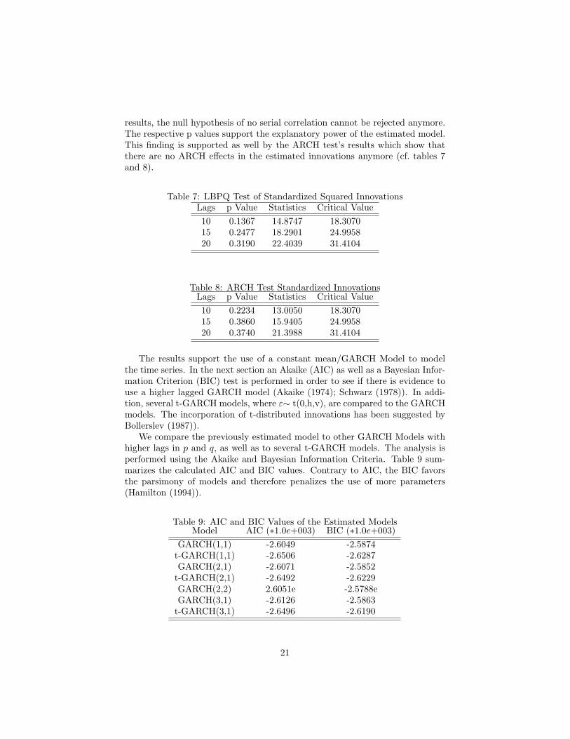
We compare the previously estimated model to other GARCH Models withhigher lags in p and q, as well as to several t-GARCH models. The analysis isperformed using the Akaike and Bayesian Information Criteria. Table 9 sum-marizes the calculated AIC and BIC values. Contrary to AIC, the BIC favorsthe parsimony of models and therefore penalizes the use of more parameters(Hamilton (1994)).

Table 9: AIC and BIC Values of the Estimated ModelsModel AIC (∗1.0e+003) BIC (∗1.0e+003)

GARCH(1,1) -2.6049 -2.5874t-GARCH(1,1) -2.6506 -2.6287GARCH(2,1) -2.6071 -2.5852

t-GARCH(2,1) -2.6492 -2.6229GARCH(2,2) 2.6051e -2.5788eGARCH(3,1) -2.6126 -2.5863

t-GARCH(3,1) -2.6496 -2.6190

21

The main result of the model comparison is that in general t-GARCH mod-els perform better than GARCH models with the assumption of normality inthe distribution of the innovations in modeling the December 2008 EUA fu-tures’ returns (cf. table 9). As far as the number of lags are concerned, thet-GARCH(1,1) model is favored over a t-GARCH(3,1) model by the relativeBIC value. The incorporation of a second ARCH term was evaluated, but therewas no statistical significance found in the estimation. Therefore, adding a sec-ond ARCH term in GARCH(2,2) is not favored over GARCH(2,1) by the AICas well as the BIC value. Thus, we concluded that a higher lagged ARCH termdoes not improve the fit of the model. The comparison of the relative BIC valueindicates that the best fit should be reached deploying a simple t-GARCH(1,1)model, although it is not favored over an t-GARCH(3,1) model by the AICvalue. However, empirical evidence suggests that the number of coefficientscorrelates negatively with the precision of the model when it comes to forecastvolatility (Hamilton (1994)). Therefore, for the selection of the model the BICvalue which penalizes the use of additional coefficients is taken as a benchmark.

The estimated parameters of the specified t-GARCH Model with p = 1 andq = 1 are presented in table 10. Again the t-statistics show that the parameters

Table 10: t-GARCH(1,1) ParametersParameter Value Std. Error t-statisitc

C 0.0019947 0.00094195 2.11ω 9.5277e-005 4.0123e-005 2.37

GARCH (1) 0.72677 0.075566 9.61ARCH(1) 0.17902 0.059341 3.01

DoF 4.0846 0.91871 4.44

are significantly different from zero. The newly estimated model therefore canbe written as:

yt = 0.0019947 + εt (4.5)

σ2t = 9.5277e− 005 + 0.17902ε2t−1 + 0.72677σ2

t−1 (4.6)

whereεt ∼ t(0, h, v) (4.7)

where h is the variance and v the degrees of freedom (DoF). The daily longterm unconditional variance of the innovations VL can be calculated by theequation VL =ω

γ (Hull (2008)). Because γ = 1-α-β= 0.09421, it follows that VL= 0.001011326. This corresponds to a daily volatility of 0.031801348.

As in the case of the GARCH(1,1) Model, the dynamics of the GARCHprocess are modeled quite good by the conditional variance. Yet, volatilityclusters in the innovations and the return can be spotted. However, the sumof the coefficients of the conditional and unconditional variance is still below 1.Moreover, with α1 + β1 = 0.90579, it is less close to the boundary conditionthan in the case of the formerly estimated model. The log-likelihood value is

22

Figure 8: t-GARCH Plot

1330.3, which is higher than in the case of the previously estimated GARCH(1,1)model.

The highly significant and rather large GARCH parameter in the modeldescribed above suggests that the persistency of the variance is quite high. Theeffect of this persistency in the variance is the observed volatility clustering.Thus, the bigger the amount of yesterday’s (t − 1) conditional volatility withrespect to the unconditional variance, the larger the contribution of yesterday’s(t0) variance term to the value of today’s variance. The value of the α parameterdescribes the reaction of the variance on shocks in the log returns. The value ofthe α in the model is rather small. This suggests that the effect of a shock inyesterday’s realization on today’s return is not very significant.

Based on the newly estimated model the values of the conditional variancesand the innovations are derived. Even though not clearly visible in the corre-lation graph, the autocorrelation was reduced in comparison to the previouslyestimated GARCH(1,1) model. According to the test results, t-GARCH(1,1)performs better in terms of the LBPQ-Test as well as with respect to theARCH-Test. The p values are significant at the 5% level (cf. table 11 andtable12). There is neither serial dependence in the innovations nor ARCH ef-fects in the standardized innovations. Investigating the autocorrelation functionof the GARCH, it can be inferred that no autocorrelation in the standardizedinnovation exists, with exception of lag four. The comparison of the results ofthe LBPQ and ARCH test show that there is no rejection of the null hypothesisof serial correlation as well as no ARCH effects at a significance level of 5%. Inthe pre-estimation analysis of the raw returns both null-hypotheses had to be

23

Figure 9: ACF of the Standardized Innovations

rejected significantly. All things considered, it can therefore be concluded thatthe model sufficiently explains the heteroscedasticity in the raw returns. Thisproves the explanatory power of the derived model.

Table 11: LBPQ Test of Standardized Squared Innovations (t-GARCH)Lags p Value Statistics Critical Value10 0.1415 14.7477 18.307015 0.2326 18.5969 24.995820 0.3052 22.6718 31.4104

Table 12: ARCH Test Standardized Innovations (t-GARCH)Lags p Value Statistics Critical Value10 0.2219 13.0310 18.307015 0.3710 16.1680 24.995820 0.3596 21.6537 31.4104

4.3 Forecasting

A times series over 170 days is forecasted using the estimated t-GARCH(1,1)and GARCH(1,1) model. The purpose of this comparison is to estimate theperformance of both models that performed best by their respective AIC values,but differ only in the assumption regarding the distribution of the innovations.After having forecasted this time series, the results are compared with their

24

counterparts derived by the Monte Carlo simulation. The returns have beenestimated using m = 20, 000 runs.

With an increasing forecasting horizon the conditional variances converge tothe long term unconditional variance. Figure10 shows that this is the fact alsoin the case of the estimated model. The asymptotic behavior of the conditionalvariance can be clearly spotted. The standard deviation of the innovations isapproaching the level of the long term unconditional variance, which was foundto be 0.031801348 or 0.029160553 in the previous section. The minimum meansquared error (MMSE) forecast lies in the middle of the standard deviation of theinnovations derived by the Monte Carlo simulation. Especially, in the very shortrun the simulated and the forecasted volatility are equal. With respect to thet-GARCH(1,1) model, the period after day 70 exhibits a greater fluctuation inthe simulated volatility. In the long run, the simulated sigmas converge towardsthe long run variance. In case of the GARCH(1,1) model, the convergence ofthe simulated and forecasted realization is better.

Figure 10: Forecast of the Model’s Standard Deviation of the ResidualsThe left panel shows the forecast of the t-GARCH(1,1) model with respect to

the simulation results. The right panned gives the same data for theGARCH(1,1) model.

Figure 11 shows that the forecasted conditional return is always 0.0019947or 0.0014831, respectively, because the expected value of the εt is zero. Thesimulated returns are evenly distributed around the mean forecast.

In figure 12 the root mean squared errors (RMSE) of the forecasted returnsare plotted with the standard deviation of the simulated returns. In general,with respect to both models, the volatility measures converge quite well. How-ever, regarding the t-GARCH model there are a few outliers, caused by theassumed student t distribution in the residuals. Furthermore, around lag 120increased volatility can be spotted.

In the following, we compare the Monte Carlo simulation output the in-sample and out-of-sample data in order to asses the predicting power of themodel using the observed data in the market. In table 13 the distributionmoments of the simulation as well as the sample figures are listed. To get anestimate of the distribution moments regarding the in-sample period, the returns

25

Figure 11: Forecasted Mean Returns and Simulated ReturnsThe left panel shows the forecast of the t-GARCH(1,1) model with respect to

the simulation results. The right panned gives the same data for theGARCH(1,1) model.

Figure 12: Standard Errors of ForecastStandard errors of forecast of the returns for the t-GARCH(1,1) model in the

left panel and for the GARCH(1,1) model in the right panel.

26

and variances have been simulated over a 590 day period. In the case of theout-of sample period, the same data as in the previous section are used.

Table 13: Distribution Momentsmean p StD Skewness Kurtosis

IS data 0.0008586 0.0278 -0.6406 6.8458OOS data 0.0016 0.0187 0.2283 4.5856Simulated GARCH IS 0.0014 0.0290 0.0037 4.7462Simulated t-GARCH IS 0.0020 0.0308 -0.6761 32.2073Simulated GARCH OOS 0.0016 0.0288 0.0135 4.1272Simulated t-GARCH OOS 0.0022 0.0310 0.7320 26.1105

The t-GARCH(1,1) model seems to have too many realizations around themean, leading to a excessively high kurtosis. Moreover, there are also a fewoutliers as observed in the RMSE comparison. In addition, the simulation out-comes are not stable. The moments of the distribution differ highly, when thenumber of simulation runs is changed. This might be because of the outliersdue to the fat tails of the distribution. Contrary, the GARCH(1,1) model seemsto have better simulation results.

Having compared the distribution moments of the in-sample and out-of-sample simulation with the sample data, it is quite astonishing that the in-sample simulation outcomes of both models are quite modest. Especially, theamount of the in-sample data’s kurtosis could not be reproduced by the model.In this respect the t-GARCH model performs quite badly. As mentioned previ-ously, the model seems to lack stability. However, regarding the GARCH modelthe outcomes are stable even if the time horizon of the simulation is changed.In addition, in terms of the out-of-sample modeling results, the GARCH modelperform well.

Based on the findings, it can be reckoned that incorporating t distributedresiduals in the model has not the intended effect regarding the fit of the model,even though the t-GARCH model performs better with respect to the Akaikeand Bayesian Information Criteria.

Following Wooldridge (2003) an additional out-of-sample comparison is made.

The RMSE is calculated according the formula√

1NΣNt=1e

2. Where e is the de-viation of the observed futures rate from the forecasted mean return. Again,20,000 different paths have been simulated, with the effect that 20,000 RMSEcould be obtained. In table 14 the mean over all 20,000 RMSEs is presented.In addition to the RMSE comparison, the mean of the relative absolute errors(MAE) of the terminal simulated errors is listed in table 14. The relative MAEcan be calculated as 1

NΣNt=1 |e|. The errors are e = yT−yT

yT. Contrary to the

RMSE where the mean of the forecasted returns is compared to the observedreturns over the whole time horizon, in the case of the relative MAE calculationonly the simulated terminal values of the futures contracts are compared to thevery last observation of the OOS data set. By doing this it is possible to get

27

an estimate about the relative errors in the last realizations of the simulatedfutures prices, which are used to calculated the derivatives’ payoff.

Table 14: RMSE between the Simulated and observed ReturnsModel RMSE MAE

GARCH 5.6210 0.3662t-GARCH 6.4849 0.4639

According to the relative comparison of the RMSE as well as the MAE of thetwo models, the GARCH(1,1) performs better than the t-GARCH(1,1) model.In the last resort and having taken into account all the findings of this section, itcan be reckoned that the simplistic GARCH(1,1) model performs best in termsof capturing the dynamics of the December 2008 futures returns.

4.4 Valuation Results

In this section we carry out the valuation of the certificates according to equation3.14. The futures rate has been simulated over the out-of-sample period fromAugust 23, 2007 until April 24, 2008, which is equal to 170 days. During thesimulation process the futures prices are tested against the knock-out barrier.This has the effect that all the price realizations which have hit the barrier arenot incorporated in the calculation of the payoff. This procedure is repeatedm =20, 000 times in order to get an reliable estimate about the derivative’s payoff. Atthe end of the simulation process the average value of the payoffs is discountedback to t0 at the risk free rate which is approximated by the Euribor adjusted for8.16 months). The outcome of this procedure is an estimate of the derivative’sprice at the beginning of the out-of-sample period or at the beginning of thelife of the option, respectively. The reason for evaluating the derivatives overthe out-of-sample period is that it allows to compare the valuation error to theerrors of the simulated futures prices declared in table 14.

It is important to note that the payoffs have to be adjusted in order to satisfythe risk neutral valuation conditions as mentioned in section 3. The risk neutralvaluation approach places a restriction on the development of the futures price.The futures price at t0 is deemed to be an unbiased predictor of the futuresrate at time T , meaning that the drift is equal to zero. In the GARCH(1,1)models’ specification, the returns are simulated by a constant plus a randomerror term. As a result the simulations of the futures returns have a mean thatis different from zero as in table 13). Thus, it is reasonable that there is a driftin the Monte Carlo Simulation, as well. Myers and Hanson (1993) suggest toadjust each terminal realization of the futures price simulation by multiplyingthe rate by the initial futures price and subsequently dividing it by the terminalrealizations’ average value. This adjustment has the effect (as shown by thecolumn (Mean FT ) in table 15), that the mean of the terminal futures pricerealizations just equals the initial futures price. Thus, satisfying risk neutral

28

valuation which requires the initial futures price to be an unbiased predictor ofthe futures rate at maturity.

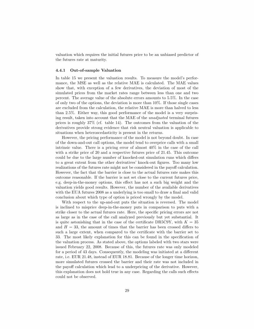
4.4.1 Out-of-sample Valuation

In table 15 we present the valuation results. To measure the model’s perfor-mance, the MSE as well as the relative MAE is calculated. The MAE valuesshow that, with exception of a few derivatives, the deviation of most of thesimulated prices from the market rates range between less than one and twopercent. The average value of the absolute errors amounts to 5.5%. In the caseof only two of the options, the deviation is more than 10%. If those single casesare excluded from the calculation, the relative MAE is more than halved to lessthan 2.5%. Either way, this good performance of the model is a very surpris-ing result, taken into account that the MAE of the unadjusted terminal futuresprices is roughly 37% (cf. table 14). The outcomes from the valuation of thederivatives provide strong evidence that risk neutral valuation is applicable tosituations when heteroscedasticity is present in the returns.

However, the pricing performance of the model is not beyond doubt. In caseof the down-and-out call options, the model tend to overprice calls with a smallintrinsic value. There is a pricing error of almost 40% in the case of the callwith a strike price of 20 and a respective futures price of 21.45. This outcomecould be due to the large number of knocked-out simulation runs which differsto a great extent from the other derivatives’ knock-out figures. Too many lowrealizations of the futures rate might not be considered in the payoff calculation.However, the fact that the barrier is close to the actual futures rate makes thisoutcome reasonable. If the barrier is not set close to the current futures price,e.g. deep-in-the-money options, this effect has not a such big weight and thevaluation yields good results. However, the number of the available derivativeswith the EUA futures 2008 as a underlying is too small to draw a final and validconclusion about which type of option is priced wrongly by the model.

With respect to the up-and-out puts the situation is reversed. The modelis inclined to misprice deep-in-the-money puts in comparison to puts with astrike closer to the actual futures rate. Here, the specific pricing errors are notas large as in the case of the call analyzed previously but yet substantial. Itis quite astonishing that in the case of the certificate DR5C9Y, with K = 35and H = 33, the amount of times that the barrier has been crossed differs tosuch a large extent, when compared to the certificate with the barrier set to33. The most likely explanation for this can be found in the specification ofthe valuation process. As stated above, the options labeled with two stars wereissued February 22, 2008. Because of this, the futures rate was only modeledfor a period of 43 days. Consequently, the modeling was initiated at a differentrate, i.e. EUR 21.48, instead of EUR 18.81. Because of the longer time horizon,more simulated futures crossed the barrier and their rate was not included inthe payoff calculation which lead to a underpricing of the derivative. However,this explanation does not hold true in any case. Regarding the calls such effectscould not be observed.

29

Tab

le15

:O

utof

Sam

ple

Cer

tific

ate

Val

uati

onR

esul

tsT

ype

Ha

Xa

Mar

ket

Val

ueb

Sim

ulat

edV

alue

e2re

lati

ve|e|

HC

ross

edM

eanFT

KN

OC

KO

UT

Cal

lsD

R5C

9Z*

75

13.5

513

.357

40.

0370

90.

0142

119

318

.81

DR

5C90

*12

108.

558.

4726

0.00

599

0.00

905

3302

18.8

1D

RO

QSR

**20

201.

31.

9056

0.36

675

0.46

585

1068

821

.48

DR

OQ

SS**

1818

3.3

3.66

080.

1301

70.

1093

344

3221

.48

DR

OQ

ST**

1616

5.3

5.49

830.

0393

20.

0374

213

6521

.48

DR

OQ

SU**

1414

7.3

7.43

160.

0173

20.

0180

331

821

.48

DR

OQ

SV**

1212

9.3

9.40

410.

0108

40.

0111

947

21.4

8D

RO

QSW

**10

1011

.311

.386

50.

0074

80.

0076

57

21.4

8M

SE/M

AE

Cal

ls0.

0768

70.

0840

9

Put

sD

R5C

9Y*

3335

15.9

513

.576

15.

6354

00.

1488

356

9418

.81

DR

98G

7*40

4526

23.7

758

4.94

706

0.08

555

2553

18.8

1D

RO

QSZ

**26

264.

24.

2476

0.00

227

0.01

133

6768

21.4

8D

RO

QS0

**28

286.

36.

3067

4.49

E-0

50.

0010

635

9321

.48

DR

OQ

S1**

3030

8.3

8.35

350.

0028

60.

0064

518

2021

.48

DR

OQ

S2**

3232

10.3

10.3

796

0.00

634

0.00

773

913

21.4

8M

SE/M

AE

Put

s0.

7975

80.

0434

9

IND

EX

TR

AC

KE

R

DR

98G

8*0

018

.28

18.2

073

0.00

529

0.00

398

18.8

1D

R1W

BM

***

00

22.6

522

.185

50.

1975

80.

0196

422

.72

AA

0G6V

I*0

018

.55

18.2

037

0.11

744

0.01

847

18.8

1H

V2C

02*

00

18.4

718

.207

30.

0690

10.

0142

218

.81

MSE

/MA

ET

rack

ers

0.09

733

0.01

408

MSE

/MA

E0.

6443

50.

0550

0

aH

=B

arr

ier,

X=

Str

ike

b*

as

of

Au

g23,

2007,

**as

of

Feb

22,

2008,

***

as

of

Oct

26,

2007.

Th

eco

rres

pon

din

gfu

ture

sp

rice

sw

ere

EU

R18.8

1,

21.4

8,

22.7

2,

resp

ecti

vel

y

30

4.4.2 Valuation up to Maturity

One possible corrective action would be to model the underlying of the shortmaturity option, labeled with ** in table 15, as well with a time horizon of170 days starting on August 23, 2007. Thus, the number of knock-outs wouldbe equal to the long maturity options. Because of the big simulation errors ofthe model,the associated problem would be that the futures price on February22, 2008, when the option began to live, were inclined to be different from thesimulated futures price. Therefore, the option would be priced wrongly evenon the first day, resulting from the simulation errors in the model. However,the results found in the previous analysis suggest that the number of knock-out events might influence the correctness of the value’s estimate. Therefore, asecond valuation is made, this time the options are valued up to their maturitywith a start date on April 24, 2008. This equals a time period of 160 days. Asthe risk free rate the Euribor rate adjusted for 7.68 months is used. The resultsof the valuation are listed in table 16.

For the down-and-out call prices, setting time horizon equal to 160 days forall simulations in the valuation of the derivatives, qualifies the very good resultsof the previously made valuation at first sight. Referring to the MSE figuresthe deviation of the model price from the market prices grew substantially. Asa consequence, the relative absolute pricing error is now slightly above 11% forthe period from April 24, 2008 until December 3, 2008 which is the maturitydate of all the knock-out options. Yet, inference about the valuation power ofthe used model may be derived based on the comparison of the outcomes whendifferent time horizons are simulated. Analyzing the valuation outcomes underscrutiny, it can be reckoned the relatively large total MAE is mainly due to theincrease of the put option price simulation’s MAE. Moreover, with respect to thecalls, using a simulation period of 160 days for all options, reduces the respectiveMAE figures by more than 3%. This is due to the fact that the pricing errors arenow more homogeneously distributed with respect to every strike price, meaningthat the range of the deviations could be reduced compared to the perviouslymade valuation as can be seen in table 3.2. The absolute errors were generallysmaller, but some big pricing errors distorted the total of MSE and MAE. Nogeneral valid inference can be made anymore which links the pricing errors tothe moneyness of the calls.

The pricing performance of the valuation regarding the up-and-out puts isvery bad with an MAE of almost 25%. In the analysis of the first valuation run,it was hypothesized that the pricing error is dependent on how many times thatthe barrier has been crossed by the simulated futures terminal realizations. Atfirst sight, this hypothesis holds true, because the number of knock-outs of theputs is much larger than the respective figures of the calls which are priced moreaccurately. However, the only put that is priced with a high accuracy is the onewith the highest knock-out figures. Thus, for the time being, this hypothesiscannot be corroborated. However, this fact needs clarification.

The pricing performance of the model regarding the index trackers in thefirst as well as in the second valuation run is very good. All results differ from

31

Tab

le16

:C

erti

ficat

eV

alua

tion

Res

ults

upto

Mat

urit

yT

ype

Ha

Xa

Mar

ket

Val

ueb

Sim

ulat

edV

alue

e2re

lati

ve|e|

HC

ross

edM

eanFT

KN

OC

KO

UT

Cal

lsD

R5C

9Z7

519

.83

18.9

088

0.84

860

0.04

645

2624

.51

DR

5C90

1210

14.8

314

.043

20.

6190

50.

0530

5578

924

.51

DR

OQ

SR20

204.

85.

3494

0.30

184

0.11

446

8713

24.5

1D

RO

QSS

1818

6.8

6.95

660.

0245

20.

0230

357

2724

.51

DR

OQ

ST16

168.

88.

6126

0.03

512

0.02

1334

1224

.51

DR

OQ

SU14

1410

.810

.346

90.

2053

0.04

1218

3224

.51

DR

OQ

SV12

1212

.812

.182

0.38

192

0.04

828

798

24.5

1D

RO

QSW

1010

14.8

14.0

791

0.51

970.

0487

125

924

.51

MSE

/MA

EC

alls

0.36

700

0.04

965

Put

sD

R5C

9Y33

359.

876.

864

9.03

604

0.30

456

1204

124

.51

DR

98G

740

4520

.96

16.2

256

22.4

1454

0.22

588

6806

24.5

1D

RO

QSZ

2626

0.9

0.82

180.

0061

20.

0868

918

592

24.5

1D

RO

QS0

2828

2.9

1.98

760.

8324

70.

3146

216

861

24.5

1D

RO

QS1

3030

4.9

3.46

082.

0712

90.

2937

114

916

24.5

1D

RO

QS2

3232

6.9

5.16

653.

0050

20.

2512

312

988

24.5

1M

SE/M

AE

Put

s6.

2275

80.

2461

5

IND

EX

TR

AC

KE

R

DR

98G

80

024

.14

23.7

562

0.14

730.

0159

24.5

1D

R1W

BM

00

24.4

23.7

562

0.41

448

0.02

639

24.5

1A

A0G

6VI

00

2523

.756

21.

5470

40.

0497

524

.51

HV

2C02

00

25.1

523

.756

21.

9426

80.

0554

524

.51

MSE

/MA

ET

rack

ers

1.01

287

0.03

686

Tot

alM

SE/M

AE

2.46

406

0.11

231

aH

=B

arr

ier,

X=

Str

ike

bas

of

Ap

r24

2008.

Th

eco

rres

pon

din

gfu

ture

sp

rice

sw

as

EU

R24.5

1

32

the observed rates by not more than 2%. This pricing error may be well tothe margins of the investment banks that have emitted theses products. Twoof the four certificates were issued by Dresdner Bank with either no maturity(DR1WBM) or with maturity date on December 3, 2008 (DR98G8), one open-end certificate by ABN Amro and one open-end certificate by Hypo Vereinsbank.Assuming that the modeled price reflects the true value of the futures, then theindex tracker DR98G8 can be seen as being priced fairly by the bank, with adeviation in its price of roughly 1.5%. This deviations might only be due tothe simulation error. In addition, this certificate had by far the lowest error inthe previous valuation run with 0.5%, as well, while the others deviated by atleast 1.5%. The other three certificates’ prices differ in the second valuation runfrom the simulated price by more than 2.5%. Theoretically, there should be nodifference in the prices because all of the four certificates track the future 2008on a 100% basis. However, it can be reasoned that in case of the three open-endcertificates, the rolling-over process should be reimbursed but this is generallydone by paying the commission when purchasing the product. However, due tothe limited amount of index tracking certificates available in the market, it isnot possible to significantly assess if the price differences among those productsare technically justifiable or intended.

5 Summary and Conclusion

The aim of this article was first and foremost to find an appropriate valuationprocedure for derivatives on EUAs. Second, the pricing of those certificatesand leveraged products should be assessed with respect to its fairness. Toachieve the first objective an investigation of the EUA futures’ price dynam-ics was undertaken. The ECX December 2008 EUA futures returns were foundto exhibit excess kurtosis and evidence of heteroscedasticity. The model estima-tion and the subsequently made performance analysis of the models, suggesteda GARCH(1,1) model to appropriately reproduce the futures dynamics. In anext step, it had to be detected if an appraisal of the respective derivatives ina risk neutral framework by deploying a Monte Carlo simulation would lead tothe right outcomes.

For short time horizons, the valuation outcomes were quite precise. Withan increased time period in the simulation the valuation’s precision is not out-standing, yet with respect to the calls and the index trackers quite good resultcould have been obtained. It can therefore be inferred that risk neutral pricing isapplicable to derivatives on EUA futures even in situations when heteroscedas-ticity is present. The small deviations of the simulated futures prices fromthe market rates are rather to be attributed to errors in the simulation of theunderlying, than to be interpreted as evidence of the not applicability of riskneutral valuation. However, it could be shown in section 4.4 that the drift inthe unadjusted simulation is responsible for the mispricing of path-dependentoptions. This drift is influencing all but the last realizations with the effect thatdisproportionately many realizations are knocked out.

33

Drawing a conclusion about the fairness of the pricing of derivatives onEUA by the issuing banks is quite hard. However, the small deviation of thevaluation results from the observed market prices regarding the participationcertificates as well as concerning the call options should provide an indicationof fair pricing. The fact that the simulated prices are generally smaller invalue in comparison to the market data can be rather attributed to errors in thesimulation process than to an intended overpricing of the options and certificatesby the issuing banks. However, it is astonishing to detect deviations of themarket value of the certificates in comparison to the futures price observedin the market. Theoretically, the certificates should mirror the futures priceon a 100% basis. In this respect the certificates issued by Dresdner Bank arepriced fairly. The respective products’ prices issued by ABN Amro and HypoVereinsbank show evidence of overpricing. Yet, due to the number of thosecertificates included in the study, a generally valid and statistically significantconclusion about the fairness of the pricing cannot be made.

The main findings of this study are in the first place, that it could be showthat risk neutral valuation is applicable in situations where heteroscedasticityis present in the underlying’s returns. Second, even tough the model is inclinedto underestimate the value of the options it can be assumed that the optionsare generally priced fairly.

References

Akaike, H. (1974): “A New Look at the Statistical Model Identification,”IEEE Transactions on Automatic Control, 19, 716–723.

Benz, E., and S. Truck (2007): “Modeling the Price Dynamics of CO2 Emis-sion Allowances,” Working Paper.

Black, F. (1976): “The Pricing of Commodity Contracts,” Journal of Finan-cial Economics, 3, 167–79.

Bollerslev, T. (1987): “A Conditionally Heteroscedastic Time Series Modelfor Speculative Prices and Rates of Returns,” The Review of Economics andStatistics, 69, 542–547.

Box, G. E. P., G. M. Jenkins, and G. C. Reinsel (1994): Time SeriesAnalysis: Forecasting and Control. Prentice–Hall, Upper Saddle River, 3rdedn.

Daskalakis, G., D. Psychoyios, and R. N. Markellos (2007): “ModelingCO2 Emission Allowance Prices and Derivatives: Evidence from the EuropeanTrading Scheme,” Working Paper.

Dickey, D. A., and W. A. Fuller (1979): “Distribution of the Estimatorsfor Autoregressive Times Series With a Unit Root,” Journal of the AmericanStatistical Association, 74(366), 427–431.

34

ECX (2008): European Climate Exchange. www.europeanclimateexchange.com.

Engle, R. (1982): “Autoregressive Conditional Heteroskedasticity with Esti-mates of the Variance of U.K. Inflation,” Econometrica, 50, 987–1008.

Geman, H. (2006): Commodities and Commodity Derivatives - Modeling andPricing for Agriculturals, Metal and Energy. Wiley, Chichester, West Sussex.

Gourieroux, C., and J. Jasiak (2001): Financial Econometrics: Problems,Models and Methods. Princeton University Press, Princeton.

Hamilton, J. D. (1994): Time Series Analysis. Princeton University Press,Princeton.

Hull, J. (2008): Options, Futures and other Derivatives. Prentice–Hall, 7thedn.

Liu, Y., and W. Enders (2003): “Out-of-Sample Forecasts and NonlinearModel Selection with an Example of the Term Structure of Interest Rates.,”Southern Economical Journal, 69(3), 520–540.

Myers, R. J., and S. D. Hanson (1993): “Pricing Commodity Options Whenthe Underlying Futures Price Exhibits Time-Varying Volatility,” AmericanJournal of Agricultural Economics, 75, 121–130.

Schwarz, G. (1978): “Estimating the Dimension of a Model,” The Annals ofStatistics, 6(2), 461–464.

Uhrig-Homburg, M., and M. Wagner (2007): “Futures Price Dynamics ofCO2 Emission Certificates. An Empirical Analysis,” Working Paper.

Wilkens, S., and P. Stoimenov (2007): “The Pricing of Leveraged Products:An Empirical Investigation of the German Market for ’Long’ and ’Short’ StockIndex Certificates,” Journal of Banking and Finance, 31, 735–750.

Wooldridge, J. M. (2003): Introductory Econometrics: A Modern Approach.South-Western, Mason, 2nd edn.

35