The UXO Classification Demonstration at San Luis Obispo, CA

I N S T I T U T E F O R D E F E N S E A N A L Y S E S

IDA Document D-4148Log: H 10-000937

September 2010

The UXO Classification Demonstrationat San Luis Obispo, CA

Shelley CazaresMichael Tuley

Approved for public release;distribution is unlimited.

About This PublicationThis work was conducted by the Institute for Defense Analyses (IDA)under contract DASW01-04-C-0003, Task AM-2-1528, “Surface and Buried UXO Detection,” for the Strategic Environmental Research and Development Program (SERDP) and Environmental Security Technology Certification Program (ESTCP). The views, opinions, and findings should not be construed as representing the official position of either the Department of Defense or the sponsoring organization.

Copyright Notice© 2010, 2011 Institute for Defense Analyses4850 Mark Center Drive, Alexandria, Virginia 22311-1882 • (703) 845-2000.

This material may be reproduced by or for the U.S. Government pursuantto the copyright license under the clause at DFARS 252.227-7013 (NOV 95).

The Institute for Defense Analyses is a non-profit corporation that operates three federally funded research and development centers to provide objective analyses of national security issues, particularly those requiring scientific and technical expertise, and conduct related research on other national challenges.

I N S T I T U T E F O R D E F E N S E A N A L Y S E S

IDA Document D-4148

The UXO Classification Demonstrationat San Luis Obispo, CA

Shelley CazaresMichael Tuley

iii

EXECUTIVE SUMMARY

BACKGROUND

Following a successful unexploded ordnance (UXO) classification demonstration

carried out at the former Camp Sibert, AL [13], the former Camp San Luis Obispo, CA,

was chosen as a second site in a series of demonstrations of increasing difficulty. The

high-level goal of the demonstration was to assess the capability of classification

algorithms, developed under the Strategic Environmental Research and Development

Program (SERDP) and refined under the Environmental Security Technology

Certification Program (ESTCP), to reliably determine which detected items could be left

safely in the ground vs. which had to be dug. This demonstration represents a further step

along the path to UXO classification, validation, and acceptance.

The intent of the demonstration was to evaluate, on a second and more

challenging live site, those instruments and algorithms that had proven successful in the

previous demonstration. As at Camp Sibert, inert UXO was seeded within the

demonstration site to provide reliable statistics on classification performance. Typically,

UXO might constitute fewer than 1% of the items dug on a live site, and with a budget

that could support approximately 2500 excavations, seeding of UXO was necessary to

allow sufficient understanding of the likelihood of false-negative classification decisions.

No additional clutter was seeded.

There was also a desire in this demonstration to test emerging advanced

instruments, as well as algorithms tailored to take advantage of the richer data set those

instruments provide. Another important goal of the demonstration was continued

involvement of the regulatory community in the design, conduct, and evaluation of all

demonstrators in an effort to better understand what might be required if detected items

that are classified as not hazardous were actually to be left in the ground.

The Institute for Defense Analyses (IDA) was assigned the responsibility to assist

ESTCP in planning, carrying out, and scoring the classification demonstration. IDA’s

principal functions were to provide seed emplacement locations and burial procedures,

create a master anomaly list, develop scoring protocols, score demonstrators’ detection

and classification results, and provide a comprehensive final report describing the

iv

demonstration. This final technical report serves as an adjunct to the summary final report

produced by ESTCP [17].

DATA COLLECTION

This demonstration used seven data-collection instruments: (1) a standard EM61-

Mk2 cart, (2) the Mobile Towed Array Detection System (MTADS) EM61 array, (3)

MTADS magnetometer array, (4) the Man-portable Simultaneous Magnetometer and

Electromagnetic System (MSEMS), (5) the MetalMapper, (6) the Time-domain

Electromagnetic MTADS (TEMTADS), and (7) the Berkeley UXO Discriminator

(BUD). The TEMTADS and the MetalMapper collected cued data over the entire survey

area, with the TEMTADS cuing off the MTADS EM61 array anomalies and the

MetalMapper off its own anomalies. The BUD collected cued data at a subset of the

TEMTADS locations.

Ten different groups submitted ranked anomaly lists for classification scoring.

These were the Army Corps of Engineers, Huntsville Center (CEHNC), Dartmouth,

Geometrics, Lawrence Berkeley National Laboratory, NAEVA, Parsons, RML, SAIC,

Signal Innovations Group, and Sky Research. Different groups provided lists for different

instruments, and sometimes multiple lists used different classification algorithms for the

same instrument. In all, 62 ranked anomaly lists were submitted, with multiple lists

submitted by some groups for a single data set. For each list, the demonstrators specified

a “don’t dig threshold.” Based on their calculations, the demonstrators believed that all

locations listed above the threshold did not have to be dug because any buried items were

not likely to be UXO and could therefore be left safely in the ground.

Careful steps were taken to prepare the site before data collection. After an

exhaustive excavation of two 50 ft 50 ft areas in a high anomaly concentration area of

the site, 60 mm mortars, 81 mm mortars, 4.2 in mortars, and 2.36 in rockets were selected

as seed items. Two hundred total seed items were emplaced, with 14 as 2.36 in rockets,

54 as 4.2 in mortars, 76 as 60 mm mortars and 56 as 81 mm mortars. In addition, during

excavation for scoring, 44 additional UXO items were dug that had not been seeded.

These included single instances of a 3 in Stokes mortar, a 37 mm round, and a 5 in

rocket, plus additional instances of types of UXO that had been seeded. The classification

demonstrators were responsible for correctly identifying the unexpected UXO types as

items to be dug.

v

RESULTS

Camp San Luis Obispo was chosen for this demonstration because, with more

difficult terrain, steeper slopes, more types of UXO, and smaller UXO, it was a more

challenging site than Camp Sibert. Results at Camp San Luis Obispo were not as

impressive as results at Camp Sibert. Taking into consideration the challenges imposed

by the site, however, the results of this demonstration clearly show that current

classification procedures could be successful on a much more difficult site than Camp

Sibert in terms of both variety of UXO and topography.

For this executive summary, only two illustrative performance curves are shown.

The first, presented in Figure ES-1, provides results achieved using survey data from a

standard EM61-Mk2 cart sensor that was analyzed using commercially available software

(UX-Process, a module within Oasis montaj). At its “don’t dig threshold,” the performer,

CEHNC, would have successfully dug all targets of interest (TOI), while leaving more

than 30% of the non-TOI in the ground.

Figure ES-1. CEHNC’s second-pass scoring results for the EM61 CART data and the UX-Process classification software. No true TOI locations rose above the don’t dig threshold

(dark-blue dot).

The second example, Figure ES-2, shows results using an advanced sensor, the

MetalMapper, and custom software developed and applied by Sky Research. While the

don’t dig threshold was incorrectly set, leaving two TOI in the ground, the near-vertical

rise of the performance curve shows that the combination of advanced sensor data and

classification algorithm could successfully distinguish most TOI from non-TOI. One of

vi

the two TOI above threshold was a 37 mm round, which was not an expected UXO item.

The other was a partial 2.36 in rocket body that also had other munition debris around it.

Multiple proximate objects continue to be difficult for current classification approaches

to handle, and performance improvement in that situation is an active area of research.

Figure ES-2. Sky’s scoring results for the MetalMapper data and the “Statistical Classifier” classification algorithm. Two true TOI locations rose above the don’t dig threshold (dark-

blue dot).

FINDINGS

The results described in this document provide a second confirmation that

successful classification is possible on a live site using currently available instruments

and software. Specific findings from this demonstration are summarized below:

Commercially available instruments and software often led to very good classification performance. The better performers using EM61-Mk2 data and UX-Analyze or UX-Process selected “don’t dig thresholds” that would have left no true TOI in the ground while reducing the unnecessary non-TOI digs by 30% to 50%.

In general, in spite of the EM61-Mk2’s limited decay-time coverage and having only four time gates, classification approaches based on principal polarizabilities and decay rate (size, shape, and wall thickness), or simply decay rate (wall thickness only) provided better performance than approaches based on comparisons of principal polarizability values alone (size and shape only).

Although there were problems with a few specific true TOI locations rising well above the demonstrators’ “don’t dig thresholds,” many of the classification

vii

performance curves for the MetalMapper and TEMTADS had a near-right-angle shape, indicating a very clear separation in feature space between true TOI and true non-TOI.

The true TOI that challenged the advanced instruments were generally portions of 2.36 in rocket bodies close to other munitions debris. For example, location #241/1475 rose above the demonstrator’s don’t dig threshold on 13 of the 14 TEMTADS ranked anomaly lists and 7 of the 10 MetalMapper ranked anomaly lists (and would have been the last true TOI recovered on 2 of the 3 ranked anomaly lists where it was below the don’t dig threshold). Other items causing problems were typically low SNR items, particularly partial 60 mm mortars buried deeply.

For the commercial EMI-based instruments, even though demonstrators typically set the don’t dig threshold somewhat aggressively (18 out of 28 ranked anomaly lists would have left at least one true TOI in the ground), 21 of the lists would have recovered over 98% of the true TOI, and all but 2 of the lists would have recovered over 95% of the true TOI.

For the advanced instruments, “don’t dig thresholds” were uniformly aggressive, with only 1 of the 29 ranked anomaly lists showing all true TOI correctly placed below the don’t dig threshold. Nevertheless, only one of the ranked anomaly lists would have recovered fewer than 95% of the true TOI. Nineteen of the 29 would have recovered more than 98% of the true TOI.

No clear metric indicated that either the MetalMapper or TEMTADS performed better than the other in this demonstration. Of the eight ranked anomaly lists for each instrument that were directly comparable, each proved superior on four (i.e., left fewer true TOI in the ground at the don’t dig threshold). Averaged over the eight ranked lists, the MetalMapper would have left 3.9 true TOI per list in the ground; the TEMTADS would have left 3.6.

ix

CONTENTS

1.  Introduction ..............................................................................................................1 

1.1  Detailed Objectives ......................................................................................2 

1.2  Demonstration Motivation ...........................................................................3 

1.3  General Approach ........................................................................................4 

1.4  Limitations ...................................................................................................8 

2.  Methods....................................................................................................................9 

2.1  Select Site...................................................................................................11 

2.2  Initial Survey ..............................................................................................13 

2.3  Select Areas ...............................................................................................15 

2.4  Excavate Sample Areas ..............................................................................15 

2.5  Generate Seed Plan ....................................................................................16 

2.5.1  Demonstration Area .......................................................................16 

2.5.2  Instrument Verification Strip .........................................................19 

2.6  Emplace Seeds ...........................................................................................20 

2.7  Collect Survey Data ...................................................................................21 

2.7.1  EM61 CART ..................................................................................21 

2.7.2  EM61 ARRAY...............................................................................22 

2.7.3  MAG ARRAY ...............................................................................23 

2.7.4  MSEMS..........................................................................................24 

2.7.5  MetalMapper ..................................................................................25 

2.8  Correct for Slope ........................................................................................26 

2.9  Detect Anomalies .......................................................................................27 

2.10  Generate Cued Lists ...................................................................................30 

2.10.1  TEMTADS .....................................................................................30 

2.10.2  BUD ...............................................................................................30 

2.10.3  MetalMapper ..................................................................................32 

2.11  Collect Cued Data at Locations on Cued Lists ..........................................33 

2.11.1  TEMTADS .....................................................................................33 

2.11.2  BUD ...............................................................................................34 

2.11.3  MetalMapper ..................................................................................35 

2.12  Generate Master List ..................................................................................35 

2.13  Select Survey Data at Locations on Master List ........................................37 

2.14  Excavate .....................................................................................................38 

2.15  Assign Ground Truth Labels ......................................................................38 

x

2.15.1  Master Locations ............................................................................38 

2.15.2  MetalMapper Cued Locations ........................................................41 

2.16  Feature extraction.......................................................................................42 

2.16.1  Classify “Can Analyze” and “Cannot Analyze” Locations ...........42 

2.16.2  Extract Features From “Can Analyze” Locations ..........................42 

2.16.3  Selecting a Subset of Features .......................................................44 

2.17  Assign Training and Test Sets ...................................................................45 

2.17.1  Standard Training Set and Standard Test Set ................................45 

2.17.2  Active Learning Training and Test Set ..........................................47 

2.17.3  Extended Training and Test Set .....................................................49 

2.17.4  The Second-Pass Training and Test Set .........................................50 

2.18  Classify Parameters ....................................................................................53 

2.19  Score Classification Performance ..............................................................56 

2.19.1  Primary Scoring .............................................................................56 

2.19.2  Secondary Scoring .........................................................................66 

3.  Results and Discussion ..........................................................................................69 

3.1  Detection Results .......................................................................................69 

3.2  Classification Results .................................................................................72 

3.2.1  Conventional Instruments ..............................................................73 

3.2.2  Advanced Instruments ...................................................................88 

4.  Findings and Conclusions ......................................................................................95 

4.1  Findings......................................................................................................95 

4.1.1  Detection ........................................................................................95 

4.1.2  Classification..................................................................................96 

4.2  Conclusions ................................................................................................98 

Appendix A: Number of Anomalies Per Instrument ...................................................... A-1 

Appendix B: Primary Scoring Results .............................................................................B-1

References ........................................................................................................................C-1

Acronyms ........................................................................................................................ D-1

1

1. INTRODUCTION

Following a successful unexploded ordnance (UXO) classification demonstration

carried out at the former Camp Sibert, AL [13], the former Camp San Luis Obispo, CA,

was chosen as a second site in a series of demonstrations of increasing difficulty. The

high-level goal of the demonstration was to assess the capability of classification

algorithms, developed under the Strategic Environmental Research and Development

Program (SERDP) and refined under the Environmental Security Technology

Certification Program (ESTCP), to reliably determine which detected items could be left

safely in the ground vs. which had to be dug. A 2003 Defense Science Board study noted

that as much as 75% of current UXO cleanup costs might be associated with digging up

nonhazardous scrap [10]. Obviously, the development, validation, and acceptance of

reliable classification instruments and algorithms have the potential to significantly

reduce UXO clearance costs or to allow more areas to be cleared for the same amount of

funding. This demonstration represents a further step along the path to UXO

classification, validation, and acceptance.

The intent of the demonstration was to evaluate, on a second and more

challenging live site, those instruments and algorithms that had proven successful in the

previous demonstration at Camp Sibert. As at Camp Sibert, inert UXO was seeded within

the demonstration site to provide reliable statistics on classification performance.

Typically, UXO might constitute 1% or less of the items dug on a live site, and with a

budget that could support approximately 2500 excavations, seeding of UXO was

necessary to allow sufficient understanding of the likelihood of false-negative

classification decisions. No additional clutter was seeded.

There was also a desire to test emerging advanced instruments, as well as

algorithms tailored to take advantage of the richer data set those instruments provide.

Another important goal of this demonstration was continued involvement of the

regulatory community in its design, conduct, and evaluation of all demonstrations in an

effort to better understand what might be required if detected items that are classified as

not hazardous are actually to be left in the ground.

Under a task titled “ESTCP/SERDP: Assessment of Traditional and Emerging

Approaches to the Detection and Identification of Surface and Buried Unexploded

2

Ordnance,” the Institute for Defense Analyses (IDA) was assigned the responsibility to

assist ESTCP in planning, carrying out, and scoring the classification demonstration.

IDA’s principal functions were to provide seed emplacement locations and burial

procedures, create a master anomaly list, develop scoring protocols, score demonstrators’

detection and classification results, and provide a comprehensive final report describing

the demonstration. This final technical report serves as an adjunct to the summary final

report produced by ESTCP [17].

1.1 DETAILED OBJECTIVES

The classification study demonstration plan [1] lays out the detailed objectives of

this demonstration:

1. Test and validate detection and classification capabilities of currently available and emerging technologies on real sites under operational conditions.

2. In cooperation with regulators and program managers, investigate how classification technologies can be acceptably implemented in cleanup operations.

Within each of these two overarching objectives are several technical sub-

objectives:

Test and evaluate capabilities by demonstrating and evaluating individual instrument and software technologies, as well as processes that combine these technologies. Compare advanced methods to existing practices and validate the pilot technologies for the following:

– Ability to detect UXO.

– Ability to identify features that distinguish scrap and other clutter from UXO.

– Ability to reduce false alarms (items that could be left in the ground that are incorrectly classified as UXO) while maintaining a probability of detection (Pd) of UXO that is acceptable to all.

– Ability to identify sources of uncertainty in the classification process and to quantify their impact to support decision-making, including issues such as impact of data quality due to how data are collected.

– Ability to quantify the overall impact on risk arising from the capability to clear more land more quickly for the same investment.

– Ability to address the issues of a dig/no-dig decision process and the related quality-assurance/quality-control issues.

3

Understand the applicability and limitations of the pilot technologies in the context of project objectives, site characteristics, and suspected ordnance contamination.

Collect high-quality, well documented data to support the next generation of signal-processing research.

This report discusses a subset of these points. The remaining points are discussed

in the summary final report produced by ESTCP [17].

1.2 DEMONSTRATION MOTIVATION

A 2003 Defense Science Board study on UXO cleanup technologies pointed out

that in a typical clearance action, more than 99% of the items dug could have been left

safely in the ground [10]. It also noted that reducing the false-alarm rate from greater than

99% to a lower, yet still relatively high, number could still save much of the cost of

clearance actions.

Significant progress has been made in classification technology as a result of

SERDP and ESTCP funding. With the exception of the initial demonstration at the

former Camp Sibert, however, testing of these approaches to date has been primarily

limited to artificially constructed test sites such as those at Aberdeen Proving Ground,

MD, and Yuma Proving Ground, AZ. Acceptance of classification technologies requires

demonstration of system capabilities at live UXO sites under real-world conditions. Any

attempt to declare detected anomalies to be harmless will require demonstrating to

regulators not only individual technologies, but an entire decision-making process. This

classification study was the second in a continuing effort that will span a number of

years. Follow-on demonstrations already in the initial planning stage at two more sites

present challenges not faced to date.

The importance of live-site testing is that the distribution of the items in the

ground before testing is realistic for UXO and clutter items. While extremely valuable,

areas such as the Aberdeen and Yuma Proving Grounds Standardized UXO Test Sites

[16] will always be somewhat artificial because both UXO and clutter items have been

emplaced in accordance with preconceived notions of how they should be distributed in

type, size, and depth, as well as location. In contrast, clutter items are not emplaced at

live sites such as Camp Sibert and Camp San Luis Obispo. Although it is usually

necessary in live-site testing to seed the area with appropriate UXO to ensure sufficient

munitions to provide reasonable statistics, the in situ clutter and any in situ UXO types

are, by definition, “real” for that site.

4

1.3 GENERAL APPROACH

The ESTCP Program Office, in conjunction with IDA and the Advisory Group of

local and state regulators, selected Camp San Luis Obispo for the second demonstration

because it met a number of desired characteristics. Historical records showed that the

portion of Camp San Luis Obispo where testing was planned likely contained 60 mm,

81 mm, and 4.2 in mortars, along with 2.36 in rockets. This made it a much more

complex site than Camp Sibert, which contained only 4.2 in mortars. In addition, the site

at Camp San Luis Obispo was on the side of a hill, providing more difficult topography

than the earlier demonstration.

Data-collection teams initially collected magnetometer array transects (widely

spaced lines of data used to assess general anomaly density in an area). Those results

guided selection of approximately 30 acres for a complete electromagnetic induction

(EMI) survey using a standard EM61-Mk2 cart. The cart results were used to select the

specific demonstration area for the study, as well as an area for the instrument

verification strip (IVS) and a test pit.

The purpose of the IVS was to confirm at the start and end of each day that all

data-collection instruments were properly functioning—that is, that they provided the

expected signal on all emplaced items, which included seed munitions and spheres. An

exhaustive excavation was performed to clear the IVS area of all metallic items before it

was seeded to ensure that only the desired signals would exist. A test pit area adjacent to

the IVS was also cleared and used to collect additional training data against expected

munition types.

In addition, two 50 ft 50 ft high-density areas were exhaustively excavated to

confirm the presence of the expected munitions types and to assess their depth

distributions. Based on the excavation results, it appeared unlikely that UXO would be

found deeper than 30 cm, and so detection thresholds were set assuming the smallest

expected signal for a target of interest (TOI) at 45 cm, providing a 50% depth margin.

As noted earlier, because of the limited number of UXO typically found (often

fewer than 1 out of 100 items excavated), it is usually necessary to seed demonstration

sites with inert UXO to provide reasonable confidence bounds on classification

performance, and seeding was necessary in this case. IDA generated a plan to seed

previously fired and inert 60 mm, 81 mm, and 4.2 in mortars, as well as 2.36 in rockets,

throughout the demonstration area and IVS. Parsons, the site-support contractor, followed

this plan and emplaced the seeds as directed. The emplacement team took care to seed the

5

items at least 3 m away from each other and from other EM61-Mk2 anomalies because

previous work has shown that current classification technologies cannot reliably analyze

multiple closely spaced items with overlapping signatures [2, 16].

Next, the data-collection teams surveyed the demonstration area using seven data-

collection instruments: (1) a standard EM61-Mk2 cart, (2) the Mobile Towed Array

Detection System (MTADS) EM61 array, (3) MTADS magnetometer array, (4) the Man-

portable Simultaneous Magnetometer and Electromagnetic System (MSEMS), (5) the

MetalMapper, (6) the Time-domain Electromagnetic MTADS (TEMTADS), and (7) the

Berkeley UXO Discriminator (BUD). The TEMTADS and the MetalMapper collected

cued data over the entire survey area, with the TEMTADS cuing off the MTADS EM61

array anomalies and the MetalMapper off its own anomalies. The BUD collected cued

data at a subset of the TEMTADS locations. Table 1 provides a brief description of each

system, with more detail provided in Section 2.

Table 1. Data Collection Systems

System Name Report

Nomenclature Sensor Description Collection Mode

MTADS EM61 Array

EM61 ARRAY

2 m × 1 m array of 3 overlapped EM61-Mk2 time domain EMI sensors with 1 m × 1 m coils firing simultaneously.

Survey

MTADS Magnetometer Array

MAG ARRAY

Eight Geometrics G-822A cesium vapor magnetometers spaced 25 cm apart and approximately 25 cm above the ground

Survey

EM61-Mk2 Cart EM61 CART Standard EM61-Mk2 cart (0.5 m × 1 m coil)

Survey

MSEMS MSEMS EM61-Mk2 cart sensor (0.5 m × 1 m coil) operated simultaneously with a G-822A cesium vapor magnetometer

Survey

MetalMapper MetalMapper Three orthogonal transmit coil time-domain EMI sensor with 7 triaxial receive coils

Survey and cued

TEMTADS TEMTADS 5×5 array of approximately 40 cm × 40 cm time-domain EMI transmit and receive coils operated multistatically

Cued

Berkeley UXO Discriminator

BUD

Three orthogonal transmit coil time domain EMI sensors with eight pairs of single-axis receive coils operating in a gradiometer mode.

Partial site cued

The data-collection teams selected detection thresholds for the survey instruments

on the basis of physics-based dipole models of the smallest expected signature collected

6

from a horizontally placed 60 mm mortar at 45 cm depth and confirmed the validity of

these thresholds using the IVS. As was recognized at the beginning of the study, different

survey instruments resulted in different anomaly detection lists. That is, many items were

detected by all instruments, some items were detected by more than one but not all

instruments, and some items were detected by a single instrument only. IDA developed

methods for reconciling the differences between individual instruments’ anomaly lists to

produce two cross-referenced master anomaly lists, one based on the EM61 array, cart,

and MSEMS anomalies and one based on the MetalMapper. Appendix A lists the number

of anomalies associated with each instrument.

Parsons, the site-support contractor, then excavated items at each location on the

master anomaly lists. Based on the excavated items, the Program Office assigned ground

truth labels to each location, with some locations assigned the label of “TOI” (target of

interest) and other locations assigned the label of “non-TOI.” IDA then separated the

locations on the master anomaly lists into a Standard Training Set and a Standard Test

Set.

Ten different groups submitted ranked anomaly lists for classification scoring.

These were the Army Corps of Engineers Huntsville Center (CEHNC), Dartmouth,

Geometrics, Lawrence Berkeley National Laboratory (LBNL), NAEVA, Parsons, RML,

SAIC, Signal Innovations Group (SIG), and Sky Research. Different groups provided

lists for different instruments, and sometimes multiple lists using different classification

algorithms for the same instrument. In all, 62 ranked anomaly lists were submitted, with

multiple lists submitted by some groups for a single data set. Demonstrator/data set

combinations are denoted with an X in Table 2.

Table 2. Data sets used by each demonstrator to provide distinct ranked anomaly lists.

Org./Data EM61 CART

EM61 ARRAY

MAG ARRAY

EM61 MSEMS

MAG MSEMS

Metal Mapper

TEM TADS

BUD

CEHNC X

Dartmouth X X

Geometrics X

LBNL X

NAEVA X

Parsons X

RML X

SAIC X X X X X

SIG X X X X X X X

Sky X X X X X X X X

7

The Program Office distributed the collected data and the master anomaly lists to

each demonstration team. The demonstrators also received the ground truth labels for all

locations in the Standard Training Set, but remained blind to the ground truth labels for

all locations in the Standard Test Set. The demonstrators used the data and ground truth

labels in the training set to optimize their inversion routines and classification algorithms.

Inversion routines are used to fit the data collected around each location on the master

anomaly list to a dipole model to estimate parameters of the buried target. Classification

algorithms are used to estimate the likelihood or probability that a buried target is a TOI

based on its estimated parameters. The demonstrators then applied their optimized

processes to the data in the test set while remaining blind to the ground truth labels. The

demonstrators created a ranked list by arranging the locations in the test set according to

their estimated probability or likelihood of being a non-TOI. Because the intent of

classification is to leave non-TOI in the ground, the ranked list is ordered from 1, the item

most likely to be non-TOI, to the highest number, the item most likely to be TOI. The

demonstrators also specified a “don’t dig threshold” that could be applied to the ranked

list, such that it was likely that all locations on the ranked list above the don’t dig

threshold were non-TOI and could therefore be left safely in the ground.

IDA scored each demonstrator’s ranked list and don’t dig threshold by comparing

the dig/don’t-dig label calculated for every location in the test set with its corresponding

ground truth label. IDA summarized the classification performance of each instrument-

algorithm combination with the metrics Percent of TOI Below Threshold and Number of

Non-TOI Below Threshold. The Percent of TOI Below Threshold is a metric similar in

concept to Pd, the probability of detection; it represents the percentage of locations with a

ground truth label of “TOI” that were correctly placed below the don’t dig threshold on

the ranked list. The Number of Non-TOI Below Threshold is simply the number of false

alarms; it represents the number of locations with a ground truth label of “non-TOI” that

were incorrectly placed below the don’t dig threshold on the ranked list.

IDA also revisited the choice of don’t dig threshold by retrospectively testing

every possible value. For each possible value of the “don’t dig threshold,” IDA

recalculated the Percent of TOI Below Threshold and the Number of Non-TOI Below

Threshold and plotted these metrics against each other to form a classification

performance curve, similar to a receiver operating characteristic (ROC) curve. The

classification performance curves and the statistics drawn from them lead to the key

findings from this demonstration. They are discussed in detail in the Results and

Discussion chapter of this report.

8

1.4 LIMITATIONS

A number of changes were implemented for this demonstration based on lessons

learned from the former Camp Sibert [13]. Even so, several limitations remain that are

the result of budget and experimental requirements:

The primary limitation was the need to seed Camp San Luis Obispo with inert munitions to obtain reasonable classification statistics. In an ideal demonstration, the area tested would be sufficiently large that valid statistics could be gained simply from recovered intact UXO. In that case, a potentially artificial distribution of UXO density, depths, and orientations is not a concern. Although 44 true UXO that were not seed items were found in the approximately 10 acres that were excavated, that still is too small a number to provide reliable statistics, and there was no assurance at the beginning of the study that even that many would be detected. Thus, to collect data from enough recovered intact UXO for valid statistics, a very large area would have to be tested. The cost of excavating all anomalies detected in such a large area would have been prohibitive. Thus, seeding was required in this demonstration, resulting in a potentially artificial distribution of UXO density, depths, and orientations. This is a limitation that is unlikely to ever be overcome in scientific testing because of funding constraints.

A second limitation was unexpected. The original plan had been to exhaustively excavate all anomalies that exceeded the detection threshold of all instruments. It was hoped that such an excavation would remain within the budget, allowing approximately 2500 anomalies to be dug. But a combination of geology and small anomalies resulted in far more magnetometer anomalies than could be dug within the budget (5266 anomalies above the MAG ARRAY threshold and 3389 above the MSEMS magnetometer threshold). Thus, excavation focused on those magnetometer anomalies that correlated with EMI anomalies. In addition, a number of apparently large, deep anomalies identified by the MSEMS magnetometer were excavated. Those excavations resulted in no metallic objects being found.

A final limitation involves the subjective judgment of what constitutes a TOI when assigning ground truth labels. In this demonstration we chose a very conservative definition and treated as TOI those items that were not only clearly munitions, but those that we felt might cause the general population concern if found. Thus, a number of the 2.36 in partial rocket bodies without warheads were treated as TOI although they had been classified by the UXO technicians as nonhazardous, and those partial rockets gave the classification demonstrators significant problems. This blurs the bright binary scoring line we preferred in a scientific experiment, but appears unavoidable in the real world.

9

2. METHODS

This chapter describes the process used to select a site for the study, select

particular areas of the site as demonstration areas, emplace seed targets in the

demonstration areas, collect data from the demonstration areas, detect anomalies in the

collected data, provide collected data and a master list of detected anomalies to the data-

processing demonstrators, and score the results of the demonstrators’ classification

outputs. Figure 1 is a flowchart of this process.

10

Figure 1: A flowchart of the UXO classification study at San Luis Obispo.

11

2.1 SELECT SITE

The first live-site UXO classification demonstration, held at the former Camp

Sibert, AL, was intentionally chosen to provide benign terrain and geology, and it

contained only one munition type, the 4.2 in mortar [13]. For the second demonstration,

the ESTCP Program Office and the Advisory Group desired a site with more challenging

topography and with a variety of munition types. The site chosen was the Rifle Range

#13 at the former Camp San Luis Obispo, CA. The site encompasses a grassy hillside

with a rock outcrop at the top and occasional isolated rocks and holes that, along with the

terrain slope, made data collection significantly more difficult than at Camp Sibert.

Figure 2, taken from the site inspection report [8], is a map of the former Camp San Luis

Obispo, CA.

Figure 2: A map of the former Camp San Luis Obispo, CA. Thick black lines outline the property boundary. Blue, red, and purple lines outline the ranges for different munition

types, according to historical records. The small green square shows the site selected for demonstration. Taken from [8].

Based on recommendations from the Advisory Group, criteria for the second

study included multiple munition types and more challenging terrain, but still relatively

benign geology. The overall site at Camp San Luis Obispo has historically included

training ranges with multiple munition types (see Figure 2). Further research by the

Program Office suggested that 60 mm, 81 mm, and 4.2 in mortars, along with 2.36 in

12

rockets, would likely be found at the particular site selected for demonstration. This site

is outlined with a small green square in Figure 2. Figure 3 shows a black-and-white aerial

photograph of this site, overlaid with a topographical map.

Figure 3: An aerial photograph of the selected site overlaid with a topographical map. Thin black lines outline large rocks at the top of a hill, and the thick black line in the southeast

corner indicates a road. The angled dark brown lines indicate fences, and the curved, light brown lines indicate topographical contours, representing 40 ft differences in elevation.

The large gray letters and large brown numbers are part of the overlaid topographical map.

13

2.2 INITIAL SURVEY

A series of surveys conducted before the demonstration provided data appropriate

for selecting the final demonstration area. Initially, total field magnetometer transect

surveys were collected at Camp San Luis Obispo and another potential site in California.

The transects at Camp San Luis Obispo covered approximately 12% of an approximate

15 ha area. Anomaly density maps were constructed from the transects and used to

narrow the potential demonstration area down to approximately 12 ha, over which a

100% coverage survey was taken using an EM61-Mk2 cart-based instrument operated by

NAEVA Geophysics, Inc. Figure 4 shows the EM61 survey map of the selected site.

Color shadings indicate the received signal amplitude at the first time gate.

14

Figure 4: The initial EM61-Mk2 cart survey map of the selected site. Colored shading indicates the sensed amplitude at the first time gate. Angled brown lines indicate fences.

Thin black lines outline large rocks at the top of the hill, and the thick black line in the southeast corner indicates a road. Blue lines outline the survey area, avoiding both the

rocky region at the top of the hill and the region of large positive amplitude in the southwest quadrant. The two red squares outline the two sample excavation areas, both in

the region of large positive amplitude in the southwest quadrant.

15

2.3 SELECT AREAS

The Program Office selected four areas of the site for specific purposes: (1) the

demonstration area where the classification performance evaluation would take place, (2)

the instrument verification strip (IVS) where the data-collection teams would calibrate

their instruments at the beginning and end of each day, (3) a test pit to allow training data

on seed items to be collected, and (4) the sample excavation areas where the Program

Office would confirm the existence of multiple munition types before the demonstration

began. An area southeast of the road was selected for the IVS because its low anomaly

density (based on EM61 CART survey) and proximity to the road would lead to a more

straightforward and efficient daily instrument calibration. A contiguous region (thick blue

line in Figure 4) was chosen for the demonstration area to allow efficient collection of

data by the vehicle-towed sensors. The rocky outcrops at the top of the hill were avoided

for the demonstration area because it would have been difficult for a number of the

instruments to collect data there. Another major criterion used to select the demonstration

area was that it could provide 250–500 anomalies per hectare, a density that would make

it likely that most anomalies consisted of individual items, allowing a reasonable

probability of classification. State-of-the-art classification technology is not advanced

enough that correct classification is likely where multiple closely spaced items occur [2,

16]. To that end, the highly dense region in the southwest quadrant of Figure 4 was not

used as a demonstration area. This region was selected for the two 50 ft 50 ft sample

excavation areas (red squares in Figure 4), however, because a large number of items

would likely be recovered, making it easier to confirm the existence of multiple munition

types.

2.4 EXCAVATE SAMPLE AREAS

The Program Office team completely excavated the sample areas to help ascertain

the potential munition types. The team recovered 369 total items from the two grids, all

buried at 30 cm depths or shallower, with subsequent EMI interrogation not indicating

more deeply buried items. In addition, the excavation team felt it unlikely that items

would be found below 30 cm, given the underlying soil composition.

Recovered items included fragments from 60 mm, 81 mm, and 4.2 in mortars.

Fuzes and unknown fragments were also recovered. No 2.36 in rocket fragments were

identified from the sample areas, although a number of 2.36 in rocket bodies were found

in the demonstration area during excavation to establish ground truth.

16

Once multiple munition types were confirmed at the site, the demonstration

proceeded to the next step: emplacing seeds in the demonstration area and instrument

verification strip.

2.5 GENERATE SEED PLAN

The seed plan consisted of a list of locations where the emplacement team was

instructed to bury inert munitions, called “seeds” [22]. The list was separated into two

sections. The first listed 200 seeds for emplacement in the demonstration area of the site.

The purpose of these 200 seeds was to guarantee the existence of a large number of TOI

to ensure sufficient statistical confidence in the classification performance metrics

eventually calculated at the end of the study. The second section listed 10 seeds for

emplacement in the IVS. The purpose of the IVS was to allow the data-collection teams

to recalibrate their instruments on a daily basis using known TOI.

2.5.1 Demonstration Area

To select the intended locations of all 200 seeds in the demonstration area, IDA

applied an amplitude threshold to the EM61 survey map to identify strong anomalies

representing geology or items indigenous to the site. Figure 5 shows the thresholded map;

blue lines outline the demonstration area. Locations with strong anomalies are shaded in

pink; all other locations are shaded in light blue. IDA visually analyzed this thresholded

map and manually selected 200 locations in the demonstration area that were far from

each other and far from any anomalies. Anomalies were avoided since multiple closely

spaced items, such as a seed emplaced next to a shell fragment, are generally difficult to

separate and classify with the state-of-the-art technology [2, 16]. Black circles mark the

intended locations of the seeds. Figure 6 is a close-up of the area enclosed by the black

square in Figure 5. Five intended seed locations are shown; all locations are far from each

other and far from any anomaly.

17

Figure 5: The thresholded EM61-Mk2 survey map with intended seed locations. Anomaly locations with a first time gate amplitude greater than 8.5 mV are shaded in pink; all other locations are shaded in light blue. Blue lines outline the demonstration area, and the thick black line in the southeast corner indicates a road. Black circles mark the intended seed locations. Two hundred seeds were emplaced in the demonstration area, and 10 seeds

formed an instrument verification strip to the southeast of the road.

18

Figure 6: A close-up of the 30 m × 30 m grid of the thresholded EM61-Mk2 survey map enclosed by the black square in Figure 5. Anomalies are common. Black circles mark the intended locations of five seeds. Each circle has a radius of 3 m. Intended locations are

further than 6 m from each other and 3 m from any anomaly.

A TOI type was then selected for emplacement at each of the 200 seed locations.

The Program Office was able to obtain many mortars from munition stores across the

United States, but estimated that it would only be able to obtain eleven 2.36 in rockets.

Therefore, eleven of the 200 seed locations were randomly selected for the 2.36 in

rockets, with the remaining 189 seed locations randomly assigned to 63 each of 60 mm,

81 mm, and 4.2 in mortars.

Next, depths were selected for the 200 seeds in the demonstration area. All seeds

were initially assigned an intended depth of 30 cm because no items from the sample

excavation areas were buried deeper than 30 cm, and the diggers thought it unlikely items

would be buried deeper. However, the program team decided to bury five 60 mm

mortars, five 81 mm mortars, and five 4.2 in mortars at 45 cm to provide some deeper

targets. No 2.36 in rockets were chosen for a depth of 45 cm because there were so few of

them.

Intended azimuth angles were selected for each of the 200 seeds in the

demonstration area. Each seed was randomly assigned to 1 of 12 groups, regardless of its

munition type. All seeds in the first group were assigned an azimuth angle of zero

degrees from magnetic north. The azimuth angle of each subsequent group was

incremented by an additional 30 degrees so that all seeds in the 12th group were assigned

an azimuth angle of 330 degrees.

19

Finally, intended inclination angles were selected for each of the 200 seeds. The

Advisory Group pointed out that most indirect-fire munitions settle in a downward

orientation. Therefore, 140 (70%) seeds were randomly assigned a downward inclination

angle, defined as within 45 degrees of pointing straight down. Similarly, 40 (20%) of the

remaining seeds were randomly chosen for a “below horizontal” inclination angle,

defined as within 45 degrees below horizontal. An “above horizontal” inclination was

chosen for the remaining 20 (10%) seeds, defined as within 45 degrees above horizontal.

Recognizing that some of the larger seeds could not be buried at a downward inclination

angle without part of the seed sticking out of the ground, the inclination angles of all

downward 81 mm mortars, 4.2 in mortars, and 2.36 in rockets were reset to below

horizontal. Only 60 mm mortars, which were small enough to remain completely buried,

were allowed to keep their initially assigned downward inclination angles.

The seed plan instructed the emplacement team to bury each seed as close as

possible to its intended location, azimuth angle, inclination angle, and depth. But the plan

also allowed for minor deviations, if needed. For example, the plan instructed the

emplacement team to inspect the ground at an intended location with a hand-held EMI

detection device before emplacing the seed to check for anomalous indigenous items or

geology that, for some reason, had failed to appear on the initial EM61-Mk2 survey map.

If there were no strong anomalies detected by the hand-held instrument within

approximately 3 m of the intended location, the seed plan instructed the emplacement

team to proceed with burying the seed. If, however, there was indeed a strong anomaly

within 3 m of the intended location, the seed plan instructed the team to choose a nearby

location for the seed. In another example, the seed plan instructed the emplacement team

to alter the depth and orientation angles of the seed if the intended parameters did not

allow at least 10 cm of dirt over the top of the buried seed. These deviations allowed for

appropriate seed emplacement.

2.5.2 Instrument Verification Strip

IDA and the Program Office manually selected the intended locations of the 10

seeds in the IVS. The Program Office recommended situating the strip directly across the

road running through the southeast corner of the site. As shown in Figure 5, this area

exhibited few anomalies representing indigenous items or geology. Furthermore, the

data-collection teams could easily access this area with their instruments at the beginning

and ending of each day. Based on that guidance, IDA selected a strip of land parallel to

and approximately 6 m southeast of the road. The seed plan instructed the emplacement

20

team to first search for, and clear this strip of, indigenous items and then emplace the 10

seeds 6 m apart from each other along the strip.

TOI locations, depths, azimuth angles, and inclination angles were selected for

each of the 10 seeds in the IVS. Two intended locations were chosen for each munition

type (60 mm mortars, 81 mm mortars, 4.2 in mortars, and 2.36 in rockets). The remaining

two locations were reserved for iron spheres (shot puts). All seeds were assigned a depth

of 30 cm. One of each type of TOI was assigned an inclination angle straight down (or as

close as possible while still allowing 5 cm of dirt over the top of the buried seed) because

downward items generally provide the strongest signal for EMI sensors. The remaining

TOI were assigned a horizontal cross-track orientation (an inclination angle directly

horizontal and an azimuth angle perpendicular to the length of the strip) because

horizontal cross-track items generally provide the weakest signals for EMI sensors.

2.6 EMPLACE SEEDS

The emplacement team followed the instructions contained in the seed plan to

emplace seeds at or near their intended locations, depths, and orientation angles, with one

exception. Upon the recommendation of the Advisory Group, the Program Office

instructed the emplacement team to choose five 60 mm mortars, five 81 mm mortars, and

five 4.2 in mortars in the demonstration area with intended depths of 30 cm and, instead,

bury them at depths of 45 cm. This doubled the number of each of these TOI types buried

at deeper depths. No 2.36 in rockets were chosen for a 45 cm depth because there were so

few of them. The emplacement team also made some substitutions into the types of TOI

buried each intended location, resulting in fourteen 2.36 in rockets (rather than the

intended 11), seventy-six 60 mm mortars (instead of the intended 63), fifty-four 4.2 in

mortars (instead of 63), and fifty-six 81 mm mortars (instead of 63).

After emplacing each seed in the ground, but before covering the seed with dirt,

the emplacement team recorded the following information:

The identification number of the seed.

The TOI type of the seed (e.g., “60 mm mortar,” “4.2 in mortar,” etc.).

The easting, northing, and height-above-ellipsoid coordinates for the nose, center, and tail of the seed, with a surveyed point on the lip of the hole providing a depth reference.

The azimuth and inclination angles of the seed.

21

A photograph of the seed, with the identification number clearly written on the seed and a ruler clearly placed next to the seed.

Once seeds were emplaced in the ground, data collection could begin.

2.7 COLLECT SURVEY DATA

The data-collection teams surveyed the demonstration area with six different data-

collection instruments. This section explains the motivation for selecting the instruments

and briefly describes the sensor technology employed by each. More detail can be found

in the plans and reports written by the data-collection teams [4, 6, 19, 21].

2.7.1 EM61 CART

The typical EMI instrument used in commercial surveys will be called the “EM61

CART” for the remainder of this document. The EM61 CART consists of a standard

EM61-Mk2 sensor mounted on a two-wheel cart. This instrument employs a 1 m × 0.5 m

receive coil mounted 30 cm above a second 1 m × 0.5 m coil that transmits as well as

receives. The instrument may be set up with four time gates from the lower coil or with

three time gates from the lower coil and the first time gate from the upper coil. The

classification demonstrators preferred the first option because it provided the maximum

temporal extent for assessing the decay characteristics of the components of the

polarization tensor.

The operator of the instrument wears a backpack containing the sensor electronics

and battery. The data-acquisition system records data (consisting of the four time gates

for the lower coil) at a rate of 16 records per second and can store up to 1 million records.

In typical commercial surveys, survey lines are often spaced 1 m apart. Because the

purpose of this study was to collect high-quality data that could support classification, the

operator was instructed to space the survey lines 0.5 m apart. Figure 7 shows the EM61

CART collecting data at San Luis Obispo.

NAEVA Geophysics, Inc., the data-collection team that operated the EM61

CART, employed a Trimble 5700 real time kinematic (RTK) differential global

positioning system (DGPS) to track the position of the sensors. Figure 7 shows the DGPS

antenna mounted above the center of the sensor coils, the standard configuration.

22

Figure 7: A photograph of the EM61 CART collecting data at Camp San Luis Obispo.

2.7.2 EM61 ARRAY

The Multi-sensor Towed Array Detection System (MTADS), developed by the

Naval Research Laboratory, was used to serially collect magnetometer and EMI data at

San Luis Obispo. Each sensor mounted on the time-domain EMI version of the MTADS

instrument (called the “EM61 ARRAY” for the remainder of this document) is a

modification of the standard EM61-Mk2 sensor sold commercially by Geonics, Ltd.

While the standard EM61-Mk2 sensor is based on a single 1 m × 0.5 m coil, the modified

sensor is based on three 1 m × 1 m coils. The three overlapping 1 m × 1 m coils are

mounted on the EM61 ARRAY, as shown in Figure 8.

Figure 8: A sketch of the three overlapping sensor coils mounted on the EM61 ARRAY.

To maximize their sensitivity, the three transmitting coils are synchronized to

provide as large a magnetic moment as possible. Based on the preference of the

classification demonstrators, the EM61 ARRAY survey was conducted in four-gate

mode, with all gates sampled on the lower coil. The sensors pulse at 75 Hz but do internal

stacking and provide an output at 10 Hz, leading to a down-track sample spacing of

15 cm for the typical 1.5 m/s survey speed. Because these are vector sensors, accurate

measurement of the orientation of the sensors is necessary for accurate data inversions.

Therefore, three RTK DGPS receivers are used to measure both the position and

orientation of the sensors at 5 Hz. A Crossbow VG300 inertial measurement unit (IMU)

23

also outputs the orientation of the sensors at 30 Hz. Figure 9 shows the EM61 ARRAY

collecting data at Camp San Luis Obispo.

Figure 9: A photograph of the EM61 ARRAY collecting data at Camp San Luis Obispo.

The EM61 ARRAY has some advantages over the EM61 CART. Its three DGPS

receivers allow the orientation of the sensor to be measured. Corrections can be made to

any errors in the sensor’s measured position caused by the tilting of the entire instrument

as it is pulled over steep terrain. The EM61 CART’s single RTK DGPS receiver does not

allow such corrections. The EM61 ARRAY also provides three cross-track samples with

excellent relative position accuracy. In contrast, the CART’s relative position from

survey line to survey line is only as accurate as its DGPS position measurements.

However, because the EM61 ARRAY’s three transmit coils fire simultaneously, items

near the center of a data line are unlikely to be illuminated by magnetic field components

in both horizontal directions. Hence the EM61 ARRAY must make a pair of surveys over

an area in orthogonal directions to ensure sufficient information for a reliable inversion.

2.7.3 MAG ARRAY

The magnetometer version of the MTADS instrument will be called the “MAG

ARRAY” throughout the remainder of this document. This instrument employs eight

Geometrics 822A total-field cesium vapor magnetometer sensors mounted in a linear

array with 25 cm spacing. The distance of the sensors above the ground is also

approximately 25 cm. The signals measured by the sensors are sampled at 50 Hz, leading

to a down-track sample spacing of approximately 6 cm for the typical 3 m/s survey speed.

A single RTK DGPS antenna is generally mounted over the center of the array and tracks

the position of the sensors at a 5 Hz sampling rate. For this demonstration, however, a

pair of DGPS antennas measured the array’s yaw and roll orientation for tilt correction.

24

(Pitch was neither measured nor corrected, although doing so would most likely have led

to a slight improvement in the accuracy of the recorded positions.) A base station receiver

placed at a surveyed monument provides DGPS corrections. Figure 10 shows the MAG

ARRAY collecting data at San Luis Obispo.

Figure 10: A photograph of the MAG ARRAY collecting data at Camp San Luis Obispo.

2.7.4 MSEMS

Under ESTCP funding, the Man-portable Simultaneous Magnetometer and

Electromagnetic System (MSEMS) was developed by Science Applications International

Corporation (SAIC) to provide a cart platform capable of collecting both EMI and

magnetometer data in a single pass. As shown in Figure 11, this is accomplished by

mounting the magnetometer on a boom that places it 4 ft ahead of a standard EM61 Mk-

2A coil. The EM61 sensor has standard wheels, so the coil is 40 cm from the ground.

Only the lower coil was installed, and data were collected from the lower coil at four time

gates. The carbon-fiber boom, supported by a third wheel, gives the Geometrics 822

cesium vapor total field magnetometer an effective height from the ground of 51 cm.

Figure 11 shows the MSEMS collecting data at San Luis Obispo.

25

Figure 11: A photograph of the MSEMS collecting data at Camp San Luis Obispo.

The MSEMS collects data simultaneously by interleaving EMI and magnetometer

collections. The EM61 is pulsed at a 75 Hz rate and outputs samples at a 10 Hz rate. For

each pulse, after EMI primary field decay and time for the magnetometer output to settle,

the magnetometer collects a static magnetic field sample. The MSEMS is pushed at a

speed of approximately 1 m/s, so with the differences in sample output rate, the EM61

provides a down-track sample spacing of about 10 cm while the magnetometer sample

spacing is about 1.3 cm. MSEMS also employs RTK DGPS, with a single antenna

between the two sensors that can be seen in Figure 11.

NAEVA operated the MSEMS at Camp San Luis Obispo with technical

assistance from SAIC. The MSEMS collected data on all grids that were scored in the

demonstration. While Sky Research used the EMI and magnetometer anomaly lists for

cooperative inversions (discussed later in this chapter), interference from local geology

made the magnetometer data not useful in many areas. However, the MSEMS pre-

processing team used the magnetometer data to identify some anomalies believed to be

deep, large targets. These were later dug, but no metallic objects were found.

2.7.5 MetalMapper

The MetalMapper is an advanced instrument developed under ESTCP funding by

Geometrics, Inc., as an enhancement to the Advanced Ordnance Locator system

developed earlier by G&G Sciences and tested under Navy funding. Figure 12 shows the

MetalMapper deployed on the front lift of a Kubota tractor. The MetalMapper instrument

employs three 1 m 1 m orthogonal transmit coils to illuminate all three target axes and

a collection of seven three-axis receive coils arranged along the bottom of the instrument

to overlap down-track and cross-track receive samples.

26

Figure 12: A photograph of the MetalMapper collecting data at Camp San Luis Obispo.

At San Luis Obispo, the MetalMapper collected survey data that were then used

to identify the locations where it should return to collect high-resolution, cued data. In

survey mode, only the horizontal transmit coil (producing a vertically directed magnetic

field) is energized, but data are collected on all receive coils. Data are collected at a

tractor speed of approximately 0.4 m/s. With a 270 Hz waveform rate and stacking to

output data at a 10 Hz rate, this produces data at about a 4 cm along-track separation.

Tracks were run with a 0.7 m separation. While the MetalMapper employs only a single

RTK DGPS receiver and antenna, it also includes an inertial measurement unit (IMU)

that allows data to be tilt corrected.

2.8 CORRECT FOR SLOPE

Survey data were collected by six different sensors at San Luis Obispo: the EM61

CART, the EM61 ARRAY, the MAG ARRAY, the MSEMS EM61 and magnetometer

sensors, and the MetalMapper. To produce a master anomaly list, anomaly declarations

from the different sensors had to be associated. Because the site was hilly and different

instruments surveyed sections in different directions, there was a concern that the

combination of the terrain slope and the vertical offset of the GPS antennas from the

sensors would result in position errors that would make anomaly association between

sensors difficult. The solution to that problem was to slope-correct the data. That could be

done with on-board information for the EM61 ARRAY, MAG ARRAY, and

MetalMapper systems, which had either multiple GPS antennas or IMUs to detect the

sensor orientation. Because the EM61 CART and MSEMS had a single GPS antenna,

their data had to be slope-corrected based on a map of terrain slope created from the

EM61 ARRAY attitude data in a two-step process [11].

27

The first step was to create a digital elevation map of the terrain that was free

from artifacts caused by small local irregularities. This was accomplished by performing

two levels of smoothing on the EM61 ARRAY GPS and IMU data. The first level used

the standard Oasis montaj gridding routine to create a minimum-curvature 1 m cell grid.

The size was chosen as a compromise between the down-track sample spacing of

approximately 0.15 m between points and the cross-track spacing of 1.5 m. The second

level of smoothing was accomplished by passing a 9 9 cell symmetric convolution filter

over the data using a standard Oasis montaj grid filter. The 9 m 9 m area was chosen to

encompass several array dimensions to remove any array orientation artifacts from the

digital elevation map.

The second step was to calculate directional grid gradients in the positive easting

and northing directions from the smoothed digital elevation map using an Oasis montaj

gradient routine. This produced a gradient map for each of the two orthogonal directions,

and these maps were employed for the slope-correction calculations. To apply the slope

correction to the recorded position of the data, the recorded position was used to look up

the gradient in each direction, and offsets in the easting and northing directions were

calculated using the gradient in that direction and the height of the GPS antenna for the

sensor in question. Although an iterative calculation that provided a better slope

correction based on the first corrected position could have been used, the average slope

correction deltas were less than 0.5 m, and it was felt that a second iteration was not

necessary. Slope-corrected data were provided to the classification demonstrators for all

the survey instruments and were also used in associating anomalies among the various

instruments when producing the master anomaly list.

Once the survey data had been corrected for tilt, individual anomalies could be

detected.

2.9 DETECT ANOMALIES

A consistent procedure for anomaly declaration was employed. Anomalies for the

EM61 CART were selected by NAEVA, for the MSEMS by SAIC, for the MetalMapper

by Snyder Geoscience, and for the EM61 ARRAY and MAG ARRAY by the Program

Office team. The major difference between the instruments was the threshold above

which an anomaly was declared. This description of anomaly selection focuses on the

EM61 ARRAY, MAG ARRAY, and MSEMS, but the procedure for all instruments

followed the same path. More detailed information can be found in the data-collection

reports for these instruments [6, 21]. Information on the EM61 CART and MetalMapper

28

anomaly-selection procedures can be found in the data-collection plans and reports for

these instruments [4, 19].

Based on the data collected from exhaustive excavation of the sample areas and

the recommendation of the Advisory Group, a maximum expected target depth of 30 cm

was selected, and a 50% depth margin was applied. To determine the anomaly-detection

threshold, we considered the physics-based predictions of the worst-case response (i.e., at

the most unfavorable orientation for the instrument) at 45 cm depth from each of the

expected munitions items. Figure 13 provides those curves for the EM61 CART and a

60 mm mortar, along with test pit measurements that show the accuracy of the worst-case

prediction curves lower bounding the expected response. Note that the second time gate

is selected for the plot; that gate was also used for detection processing. While the target

signal is stronger in the first gate, the signal-to-noise ratio (SNR) is frequently larger in

the second or third gates because of their improved immunity to motion noise.

Figure 13: The expected EM61 CART second time gate amplitude for the most unfavorable orientation as a function of distance below the transmit coil for a 60 mm mortar and

measured data from the test pit.

Given the threshold for a particular instrument, detection processing first

consisted of selecting peaks in the gridded data that exceeded the chosen threshold. Other

than gridding the data, no data smoothing was performed before anomaly selection.

Actual anomaly selection was accomplished using the gridpeak function in Oasis montaj.

Distance Below Lower Coil (cm)

40 60 80 100 120 140 160 180 200

Pea

k S

igna

l (m

V)

1

10

100

1,000

10,000

Depth (cm) assuming Standard Wheel Mounting

0 20 40 60 80 100 120 140 160

least favorable orientationtest pit measurements - gate 2detection threshold

Gate 2RMS Noise

Depth of Interest

29

Once the list of anomalies and their locations was produced, the instrument data

were imported into the UX-Analyze module of Oasis montaj so that the anomalies could

be inverted using a dipole model. A chip of data surrounding the anomaly peak that

encompassed the anomaly was either extracted automatically or a polygon surrounding

the desired data was generated manually for data inversion. UX-Analyze provides a

picture of the gridded data along with the match data produced by the inversion

parameters; fit coherence values; and fit parameters, including the location and depth of

the object. The data analyst checks those parameters as part of the overall quality-control

process. If the fit location passes the quality check, it is returned as the anomaly location.

For items with a poor fit, the grid location of the anomaly peak is returned instead.

For elongated items, particularly those elongated in the down-track direction,

EM61-based instruments can provide a double-humped return for a single item. For this

experiment, the data analyst looked at all anomalies that were within 0.6 m of each other

to determine whether they came from a single item or from multiple closely spaced items.

In the cases where it was judged that the returns constituted a single unique anomaly, it

was treated as such on the anomaly list.

Determining anomalies for the magnetometer data followed a similar procedure as

that for the EM61-based instruments, but there were differences due to the physics that

determines the response for the two types of instruments. Magnetometers sense the

distortion in Earth’s magnetic field due to the presence of a ferrous object. For most

target aspects relative to Earth’s field, this distortion presents itself as a bipolar field

distortion. This field distortion at the instrument can be predicted using physics models

analogous to those for the EM61-based instruments. Such models were used to establish

the threshold for detection by the magnetometers, using the same 50% depth safety factor

as for the EMI case. Actual anomaly detection selection was based on the positive peak

of the anomaly, but the anomaly location reported was that given by a dipole inversion.

Adverse geology at the Camp San Luis Obispo site caused the magnetometer

threshold to be exceeded in a number of instances, many of which were not near an EMI

anomaly. For that reason, the only magnetometer anomalies prosecuted in the excavation

phase of the demonstration were those that associated with an EMI anomaly, plus 45

additional excavations for what the MSEMS pre-processor felt might be large, deeply

buried items. (The demonstrators did not attempt to classify these additional 45

anomalies, however. Furthermore, no metallic items were recovered from these

anomalies during excavation.) Because the geology of the site was highly magnetic in

30

some areas, many more anomalies were detected in the magnetometer-based survey data

than in the EM61-based data.

Once the data-collection teams had detected individual anomalies in the survey

data, other data-collection teams could collect high-resolution, cued data at individual

locations throughout the site.

2.10 GENERATE CUED LISTS

The cued lists provided the data-collection teams with the locations of high-

resolution data to be collected with the cued instruments. Three cued lists were formed,

one for the TEMTADS, the BUD, and the MetalMapper, the three cued instruments used

at Camp San Luis Obispo.

2.10.1 TEMTADS

IDA created the TEMTADS cued list from the EM61 ARRAY anomaly list. The

1464 locations on the TEMTADS cued list corresponded to the 1464 unique anomalies

detected by the EM61 ARRAY. The Program Office team fit the data from each EM61

ARRAY anomaly to a dipole model using the UX-Analyze module in Oasis montaj. IDA

included an anomaly’s fitted location on the TEMTADS cued list if the anomaly’s data:

Exhibited a fit coherence greater than or equal to 0.85, and

Based on the Program Office team’s visual analysis:

Fit well to the dipole model,

Appeared to represent a single buried item, and

Encompassed the complete anomaly.

Conversely, the location of the anomaly’s peak signal was included on the TEMTADS

cued list, rather than its fitted location, if the anomaly’s data:

Exhibited a fit coherence less than 0.85, or

Based on the Program Office team’s visual analysis:

Appeared to fit poorly to the dipole model,

Appeared to represent multiple closely spaced items, or

Did not encompass the complete anomaly.

2.10.2 BUD

The BUD cued list was a subset of the TEMTADS cued list. BUD remains in the

early phase of development, and its large size and weight cause difficulties in

31

transporting it from one cued location to another, especially over steep terrain. The

Program Office decided in advance that the BUD would collect data only at locations

with relatively flat terrain. To that end, two contiguous sub-areas of the site that were

relatively flat were identified, and all TEMTADS cued locations in these sub-areas were

assigned to the BUD cued list. Figure 14 is a topographical map of the site. Blue lines

outline the survey area, and the curved light-brown lines indicate topographical contours.

Orange dots show locations where both the TEMTADS and BUD collected cued data; all

are within relatively flat sub-areas of the site. Purple dots show locations where only the

TEMTADS collected cued data; the terrain was quite steep in these locations.

32

Figure 14: A topographical map of the selected site with TEMTADS and BUD cued

locations. Blue lines outline the demonstration area, and the curved light-brown lines indicate topographical contours with elevation differences of 40 ft. Orange dots show

locations where both the TEMTADS and BUD collected cued data; all are within relatively flat sub-areas of the site. Purple dots show locations where only the TEMTADS collected

cued data; the terrain was quite steep in these areas.

2.10.3 MetalMapper

The MetalMapper data-collection team created the MetalMapper cued list

independently of the TEMTADS and BUD cued lists. As discussed in the data-collection

report [19], the data-collection team surveyed the site with the MetalMapper in dynamic

33

mode. The team detected 1617 unique anomalies in the MetalMapper survey data and

included the locations of each of these anomalies on the MetalMapper cued list. Cued

data were eventually collected at all 1617 locations on the MetalMapper cued list. But the

classification demonstrators processed the data recorded at only 1561 cued locations

because 56 locations were not excavated in time to provide ground truth labels used for

optimizing the classification algorithms.

2.11 COLLECT CUED DATA AT LOCATIONS ON CUED LISTS

In collecting cued data, TEMTADS, BUD, and MetalMapper used different sets

of cued locations. This section describes the sensor technology of the instruments. More

detail can be found in the reports written by the data-collection teams [5, 14, 19].

2.11.1 TEMTADS

TEMTADS, an advanced sensor constructed by the Naval Research Laboratory, is

based on the coils and electronics from the Advanced Ordnance Locator system,

developed under Navy funding by G&G Sciences. As shown in Figure 15, TEMTADS

employs twenty-five 35 cm square sensors arranged in a 5 5 array. Each sensor consists

of a 35 cm square outside transmit coil and a 25 cm square inner receive coil. The coils

are mounted on 40 cm centers, forming a 2 m 2 m array.

Figure 15: A sketch of the transmit/receive coils mounted on the TEMTADS.

Each transmit coil is sequentially pulsed, with the induced secondary field from

any item below the array sensed by all 25 receive coils. This arrangement provides spatial

transmit and receive diversity, along with the additional information provided by multi-

static operation. As a cued sensor, TEMTADS can do sufficient signal stacking to

34

produce high SNR data. In addition, the increased sensitivity provided by stacking allows

extension of the receiver processing time to 25 ms, giving a good sampling of the late-

time decay for large, thick-walled objects. Sampling is done at 250 kHz, but data for

analysis consist of 115 logarithmically spaced gates covering 40 s to 25 ms.

At Camp San Luis Obispo, TEMTADS collected cued data at all the unique

anomaly locations produced from the EM61 ARRAY survey. The procedure was to

program anomaly locations into the TEMTADS navigation software, drive the tow

vehicle to place the center of the array over the anomaly, collect data, and then move to

the next anomaly. Quality control checks were subsequently performed on the collected

data to allow anomalies to be revisited if necessary. Figure 16 shows the TEMTADS

collecting data at San Luis Obispo.

Figure 16: A photograph of TEMTADS collecting data at Camp San Luis Obispo.

2.11.2 BUD

BUD is a next-generation instrument developed by Lawrence Berkeley National

Laboratory. Its design and construction were funded by ESTCP and SERDP. BUD is still

a developmental instrument and data collection is slow, so it collected data in only the

cued mode. Figure 17 shows the BUD collecting cued data at Camp San Luis Obispo. For

this collection, the BUD operators chose to collect data at 11 points relative to the flagged

anomaly, 5 points at half-meter intervals with the center point over the anomaly, and 3

points in lines offset.

35

Figure 17: A photograph of the BUD collecting data at Camp San Luis Obispo.

The BUD consists of three orthogonal transmit coils and eight pairs of receive

coils that are differenced to provide a gradiometer output. The eight pairs of receive coils

are mounted diagonally across the upper and lower horizontal transmit coils to provide

gradiometric samples along the three axes. In cued mode, the BUD sequentially pulses all

three transmit coils to fully interrogate the source of the anomaly. The BUD samples at a

rate of 250 kHz and has 35 sample gates logarithmically spaced from 153 µs to 1387 µs.

Because the BUD remains temporarily stationary while collecting data, time is available

for data stacking, and motion noise is suppressed. This leads to an improved SNR, which

in turn leads to more accurate data inversions.

2.11.3 MetalMapper

For this demonstration, the MetalMapper was self-cued from a list of anomalies

detected in the data it collected itself in survey mode. Thus, the MetalMapper

demonstration took place independently of the demonstration of the other instruments. In

cued mode, the MetalMapper was driven to the anomaly location and lowered so that the

bottom skids were on the ground. Data were collected by sequentially exciting each of

the three transmitter coils. Data were collected at a 30 Hz rate, and 270 repetitions were

stacked for each transmitter to improve SNR.

Once data were collected by all survey and cued instruments, preparations began

for excavating each detected anomaly to provide ground truth for scoring.

2.12 GENERATE MASTER LIST

The master list consisted of the union of all survey instruments’ anomaly lists and

all cued instruments’ cued lists. The purpose of the master list was to develop a single

36

excavation list and to allow for a straightforward scoring process. The master list

instructed the classification demonstrators where to extract features from the collected

data; the demonstrators then classified each location based on its extracted features. The

master list also instructed the excavation team where to recover buried items; the

Program Office then assigned one ground truth label to each master location based on the

characteristics of its recovered item or items. IDA scored the demonstrators’

classification performance by comparing each location’s classification output with its

ground truth label.

The master list was constructed in three sequential steps. In the initial step, the

first 1464 locations on the master list were defined as the 1464 locations on the

TEMTADS cued list, corresponding to the 1464 unique anomalies detected by the EM61

ARRAY. In the second step, an additional 355 master locations were taken from the

fitted locations of 355 of the 1552 unique anomalies detected by the EM61 CART. These

355 anomalies had fitted locations further than 0.6 m from any of the master locations

from the first step. In the third step, an additional 387 master locations were added from

387 of the 1561 unique locations on the MetalMapper cued list. These 387 cued locations

were further than 0.6 m from any of the master locations already designated in the first

and second steps. The remaining MetalMapper anomalies fell within 0.6 m of a location

added to the list in the first or second step. Thus, the master list consisted of a total of

2206 locations (1464 + 355 + 387).

The Program Office briefly considered appending additional locations to the

master list in a fourth, fifth, and sixth step. The fourth step would have added an

additional 614 master locations from 614 of the 2316 unique EM61 MSEMS anomalies

whose fitted locations were further than 0.6 m from any of the master locations created in

the first three steps. The Program Office quickly abandoned this idea due to the

prohibitive cost of recovering items from over 600 additional locations. The fifth and

sixth steps would have added master locations from MAG MSEMS and MAG ARRAY

anomalies whose fitted locations were further than 0.6 m from any previously formed

master location. This idea was also abandoned because the magnetic geology of some

areas of the site made magnetometer-based survey instruments unsuitable for anomaly

detection.

IDA associated each of the 2206 master locations with one or more instruments,

with the exception of the MetalMapper. Specifically, a master location was associated

with a cued instrument if the instrument collected cued data within 0.6 m of the master

location. Similarly, a master location was associated with an EM61-based survey

37

instrument if there was at least one anomaly detected by the instrument whose fitted

location was within 0.6 m of the master location. The same approach could not be used to

associate master locations with magnetometer-based survey instruments, however,

because the magnetometer-based surveys led to the detection of many overlapping

anomalies. Therefore, a master location was associated with the MAG ARRAY if it had

already been associated with the EM61 ARRAY. Similarly, master locations were

associated with the MAG MSEMS sensor if they were already associated with the EM61

MSEMS sensor. No master locations were associated with the MetalMapper because the

MetalMapper classification demonstration was held independently of the rest of the

study. The table in Appendix A shows the number of locations associated with each

instrument.

Once the master list was created, the classification demonstrators could begin

processing data at each location on the master list.

2.13 SELECT SURVEY DATA AT LOCATIONS ON MASTER LIST

Data collected with cued instruments differ in nature from data collected with

survey instruments. A cued instrument collects many individual sets of data, with each

set collected over one location on the instrument’s cued list. In contrast, a survey

instrument collects a single large set of data over the entire demonstration area of the site.

In this study, the classification demonstrators had to select from this large set of survey

data many individual smaller subsets of data, with each subset corresponding to one

location on the master list. This process was one of the most subjective steps in the entire

study.

The demonstrators selected survey data around individual master locations. First,

they visually analyzed the survey data surrounding each master location associated with a

given instrument. Then, they selected a polygon circumscribing the master location. The

polygon was intended to capture only those data points representing the detected

anomaly, so that only the data representing the anomaly, rather than background, would

be analyzed further. For master locations associated with more than one survey

instrument, the demonstrators selected different polygons for different instruments

because the data collected by some instruments were of a higher resolution or SNR than

the data collected by other instruments.

While the demonstrators were analyzing the collected data, the Program Office

was taking steps to assign ground truth labels to the collected data.

38

2.14 EXCAVATE

The excavation team recovered all items buried at the master locations. The

purpose of the excavation was to gather ground truth information that could be used to

score the output of the demonstrators’ classification analyses. As it turned out, multiple

items were recovered from some master locations, while no items were recovered from

other locations. Upon uncovering an item, but before removing it from the ground, the

excavation team cataloged the following information:

The easting, northing, and depth coordinates for the center of the item, with depth measured with respect to a surveyed point on the lip of the hole.

A description of the item (e.g., “60 mm mortar,” “fin parts,” “scrap metal,” etc.).

A photograph of the item, with a ruler and a small white board clearly placed next to the item. The excavation team wrote the master location’s identification number on the white board. Figure 18 shows photographs of different recovered items.

The excavation team recovered all 200 seeds that had been emplaced in the

survey area, along with hundreds of clutter items (including parts of previously exploded

munitions), as well as 44 intact or nearly intact munitions that were indigenous to the site.

Some of these indigenous munitions—one 5 in rocket, one 3 in Stokes mortar, and one

37 mm round—were unexpected because historical records did not indicate that these

types of munitions had been fired at the site.

2.15 ASSIGN GROUND TRUTH LABELS

The Program Office and IDA assigned a single ground truth label to each master

location, as well as to each MetalMapper cued location. Each label was based on the

characteristics of the item or items recovered at the location.

2.15.1 Master Locations

The Program Office assigned one ground truth label to each location on the

master list. Specifically, a location was labeled as “TOI” if any item recovered from the

location was a seed; an intact munition indigenous to the site; or any item that a

reasonable individual might suspect to be an explosive munition, based on the excavation

team’s description and photograph of the item. Conversely, a master location was labeled

as “non-TOI” if no items recovered from the location met these criteria. In addition, all

locations labeled as “TOI” were further labeled by type (e.g., “60 mm mortar,” “81 mm

39

mortar,” etc.). As it turned out, no more than one TOI was recovered from any one

location.

Some locations were difficult to label. The Program Office questioned whether a

reasonable individual might suspect some partial munitions to be explosive, such as those

shown in Figure 19. To settle the matter, photographs of questionable items recovered

were gathered from locations that had been assigned to the Standard Training Set. (The

training and test sets will be discussed later in this chapter.) These photographs were

presented to both the Advisory Group and the classification demonstrators, and these

groups were asked for their opinion. After much debate, the Program Office, the

Advisory Group, and the classification demonstrators labeled each questionable location

in the training set as “TOI” or “non-TOI.” For example, they labeled the training set

location in Figure 19(a) as “TOI,” since they believed a reasonable individual would

suspect the item to be an explosive munition. Much of this was because the item still

retained many of its fins, which can appear dangerous to a reasonable, yet untrained,

individual. The Program Office then applied the same logic to each questionable location

in the test set, labeling each of these as “TOI” or “non-TOI” in a manner consistent with

the training set. (The Program Office did not ask for the demonstrators’ opinions

regarding the questionable locations in the test set because the demonstrators remained

blind to the ground truth labels in the test set throughout the course of the study.) For

example, the Program Office labeled the test set location in Figure 19(b) as “TOI”

because the recovered item resembled the item shown in Figure 19(a).

40

(a) (b)

(c) (d)

(e) (f)

(g) (h)

Figure 18: Photographs of recovered items, including (a) a 60 mm mortar, (b) an 81 mm mortar, (c) a 4.2 in mortar, (d) a 2.36 in rocket, (e) a 5 in rocket, (f) a 3 in Stokes mortar, (g)

a 37 mm round, and (h) scrap metal from a previously exploded munition.

41

(a) (b)

Figure 19: Photographs of questionable items excavated from (a) a training set location and (b) a test set location. After much debate, the Program Office, the Advisory Group, and

the classification demonstrators labeled the training set location in (a) as “TOI” because they believed a reasonable individual would suspect the recovered item to be an explosive munition. To maintain consistency, the Program Office also labeled the test set location in

(b) as “TOI” because the recovered item bore a close resemblance to the item shown in the first photograph.

The Program Office erred on the side of caution when assigning ground truth

labels to questionable locations, more often labeling a questionable location as “TOI”

than as “non-TOI.” In a real-world situation, a partial munition that remained in the

ground poses no true threat to public safety since it can no longer explode. But a

reasonable individual who found the munition could perceive it as a threat, leading to

costs associated with public relations and any potential police or explosive ordnance

disposal response to 911 calls.

2.15.2 MetalMapper Cued Locations

IDA also assigned a single ground truth label to each MetalMapper cued location.

The MetalMapper demonstration occurred independently of the other parts of the study,

and not all MetalMapper cued locations mapped directly to a master location. Therefore,

for each MetalMapper cued location, all master locations within 0.6 m of the cued

location were identified. Most cued locations had only one master location within 0.6 m.

These cued locations were assigned the ground truth label of the associated master

location. However, some cued locations had more than one master location within 0.6 m.

Only one of the associated ground truth labels were assigned to each of these cued

locations, with TOI taking precedence over non-TOI. As it turned out, no cued locations

were associated with more than one master location labeled as TOI.

While the Program Office and IDA assigned ground truth labels to the master

locations and MetalMapper cued locations, the classification demonstrators were further

analyzing the data collected at these locations.

42

2.16 FEATURE EXTRACTION

The classification demonstrators processed the data collected at each location

associated with a given instrument. First, the demonstrators classified each location as

“Can Analyze” or “Cannot Analyze.” Then, they extracted features from the “Can

Analyze” locations; most demonstrators extracted these features by fitting the collected

data to a dipole model. Finally, they selected a subset of the extracted features on which

further, more specific classification could be based.

2.16.1 Classify “Can Analyze” and “Cannot Analyze” Locations

The demonstrators classified a given location as “Can Analyze” or “Cannot

Analyze” based on the quality of data recorded at that location. The data recorded from

most instruments at most locations were of sufficient quality for accurate feature

extraction. In these cases, the demonstrators classified the locations as “Can Analyze.” In

contrast, the data recorded by some instruments at some locations suffered from

geolocation errors, spotty coverage, low data density, or low SNR, making it difficult, if

not impossible, to extract accurate features. In such cases, the demonstrators classified

these locations as “Cannot Analyze.”

Different demonstrators used different criteria for making the “Can Analyze” or

“Cannot Analyze” classification. While some demonstrators used quantitative criteria,

such as the fit coherence or a similar measure of how well the collected data fit to a

dipole model, other demonstrators used subjective criteria, such as visual analysis of the

collected data. Furthermore, in many cases, the same demonstrator classified a location as

“Can Analyze” based on one instrument’s data but as “Cannot Analyze” based on another

instrument’s data because different instruments have different resolutions, SNRs, etc.

2.16.2 Extract Features From “Can Analyze” Locations

The demonstrators extracted features from each location classified as “Can

Analyze.” Most demonstration teams extracted geophysical parameters, estimating the

characteristics of the item(s) that were likely to be buried at the location, based on a

dipole model of the data collected at the location. In contrast, some demonstration teams

extracted features that were related to direct measurements of the collected data itself.

2.16.2.1 Extract Features: Geophysical Parameters of Dipole Models

To estimate parameters of the item(s) buried at a location, demonstrators input the

data collected at the location into a geophysical inversion computer routine. This routine

43

fit the data to a dipole model. Parameters of the best fit dipole model were then used in

classification processing.

Different demonstration teams used different inversion routines. Some routines

assumed that only a single item was buried at each location, an assumption that was not

always true. Other demonstrators used more complex routines that estimated the number

of buried items as well as their parameters. Despite their differences, however, all

inversion routines estimated intrinsic and extrinsic parameters of the buried item(s).

Extrinsic parameters included a buried item’s easting and northing coordinates, as well as

its orientation angles and depth. Intrinsic parameters included characteristics of the buried

item—size, shape, material composition, and wall thickness—regardless of where or how

the item was situated. The data-processing demonstrators designed their classification

algorithms to exploit the known differences in intrinsic parameters between TOI and non-

TOI.

Inversion routines operating on EMI data can estimate many intrinsic parameters.

For example, the inversion routines applied to standard EM61-Mk2 sensor data estimate

the polarizability of the buried item along each of its three major axes (1, 2, 3) at three

or four different time gates. The amplitudes of the polarizabilities indicate the item’s size,

and their relative amplitudes with respect to each other indicate the item’s shape. TOI

tend to be ferrous bodies of revolution with one large axis and two equal, smaller axes. In

contrast, non-TOI, such as munitions debris and cultural items, can be very small and are

not often bodies of revolution. More advanced EMI sensors, such as those used on the

TEMTADS and MetalMapper, sample the received signal at later time gates than the

standard EM61-Mk2. Their inversion routines estimate the polarizabilities of the buried

item over a longer span of time, such that the polarizabilities’ decay rates () can be

estimated. Decay rates indicate the item’s material composition and wall thickness, with

TOI tending toward thicker walls than non-TOI.

Inversion routines applied to magnetometer data can estimate fewer intrinsic

parameters. To estimate the three polarizabilities of a buried item—that is, to estimate its

shape as well as its size—the item must be illuminated and sampled from three

orthogonal directions. Magnetometers cannot always accomplish this because they rely

on Earth’s magnetic field to illuminate the item; there is no assurance that this field will

sufficiently illuminate all three axes of the item at once (e.g., if an item was aligned with

Earth’s magnetic field, no information about the other two axes could be estimated).

Magnetometers can only estimate the item’s magnetic moment (induced plus remanent)

which gives the item’s effective size in the illumination direction only.

44

“Cooperative” inversions can also be performed using EMI and magnetometer

data recorded at the same location. Although EMI inversions provide more information

than magnetometer inversions, magnetometer inversions often lead to more accurate

depth estimates. Cooperative inversions enjoy the advantages of both. Demonstrators first

invert the magnetometer data to estimate the buried item’s depth as accurately as

possible. Then, they invert the EMI data with the depth parameter of the EMI dipole

model constrained to the value previously estimated using the magnetometer model.

Constraining the value of one parameter reduces the number of degrees of freedom of the

EMI model. If the parameter is constrained to an accurate value, the reduction in the

number of degrees of freedom increases the likely accuracy of the other estimated

parameters. One demonstration team, Sky Research, performed cooperative inversions in

this study using the EM61 and MAG MSEMS data. Other demonstrators chose not to

perform cooperative inversions because the highly magnetic geology of the site made the

magnetometer data difficult to analyze.

2.16.2.2 Extract Features: Data-Driven

Some demonstration teams did not estimate the characteristics of the item buried

at a location. Instead, they measured the characteristics of the anomaly to which the

buried item gave rise. Examples of these measurements include the peak amplitude of the

anomaly, the footprint area of the anomaly, and the time decay of one channel of data

recorded at the anomaly (rather than the time decay of a polarizability parameter of a

dipole model that was fitted to the data). Unlike the geophysical parameters resulting

from dipole model inversions, these data-driven features do not directly describe the

intrinsic parameters of the buried item(s). Some have hypothesized that these data-driven

features can still be used for accurate classification, however.

2.16.3 Selecting a Subset of Features

For a given instrument, the demonstrators chose a subset of the extracted features

likely to best exploit the known differences between TOI and non-TOI locations. The

demonstrators formed a feature vector from the chosen subset, with each element of the

vector holding one of the chosen features. Some demonstrators chose a very simple

subset consisting of a single feature only, such as the magnetic moment or the principal

polarizability at one time gate. This resulted in a one-dimensional feature vector. Other

demonstrators chose more complex subsets consisting of multiple combinations of

multiple parameters, such as the ratio of a polarizability decay rate to the polarizability

45

amplitude. This resulted in a multidimensional feature vector. In either case, the

demonstrators used the feature vectors to further classify the locations.

Before classification could proceed further, however, the collected data were

separated into training and test sets.

2.17 ASSIGN TRAINING AND TEST SETS

IDA assigned each master location and each MetalMapper cued location to either

a Standard Training Set or Standard Test Set. Training and test sets serve complementary

purposes. A training set allows demonstrators to optimize their classification algorithms

using a subset of data labeled with ground truth. To that end, the Program Office released

to the demonstrators all ground truth information related to the Standard Training Set

locations so that the demonstrators could use these labels to optimize their algorithms.

(Demonstrators could also choose to use the data and ground truth labels from the TOI

seeded in both the IVS and the test pit.) The Standard Test Set allows demonstrators to

test their optimized algorithms by applying the algorithms to the remaining, unlabeled

data. As such, the Program Office did not release ground truth information related to the

Standard Test Set locations. In this way, the demonstrators’ analyses of the Standard Test

Set locations were kept “blind.”

2.17.1 Standard Training Set and Standard Test Set

Most demonstrators used the Standard Training Set and Standard Test Set to

optimize and test their classification algorithms. The survey site consisted of forty-five

30 m 30 m grids. IDA selected six of these grids and assigned to the Standard Training

Set all locations residing in these grids. All remaining locations were assigned to the

Standard Test Set. The six Standard Training Set grids were selected from different sub-

areas of the site. (Two of the six grids were located in the sub-areas of the site over which

the BUD collected data, shown in Figure 14. This was done such that the training data

available for BUD-related analyses were a subset of the training data used for all other

instruments’ analyses.) Figure 20 shows a topographical map of the site with master

locations plotted as dots. (Only those master locations associated with the EM61 ARRAY

are shown.) Those locations residing in the Standard Training Set grids are colored in red

and green, depending on their ground truth label. The locations residing in the Standard

Test Set grids are colored in black, regardless of their ground truth label.

46

Figure 20: A topographical map of the site with master locations associated with the EM61 ARRAY in the Standard Training Set and Standard Test Set. The blue lines outline the

demonstration area. Red and green dots mark the true TOI and non-TOI locations in the Standard Training Set. Black dots mark the locations in the Standard Test Set, regardless

of ground truth label.

Unlike most demonstrators, Signals Innovations Group (SIG) used both

traditional and novel techniques for training and testing their classification algorithms.

The traditional technique was supervised learning; like the other demonstrators, SIG

optimized its algorithms using the ground truth labels in the training set and then applied

the optimized algorithms to the test set. The novel technique was semi-supervised

47

learning. With semi-supervised learning, SIG optimized its algorithm using labeled data

from the training set, as well as unlabeled data from the test set. Then, SIG tested the

optimized algorithm by applying it to only the unlabeled data in the test set.

2.17.2 Active Learning Training and Test Set

SIG also used active learning [12]. Active learning, an alternative approach for

constructing a training set, is used in conjunction with either supervised or semi-

supervised learning techniques. With active learning, the training set is not determined in

advance. Instead, all locations are initially unlabeled, and the demonstrators use

information-theory metrics to identify from which locations the optimization could

benefit most if ground truth labels were assigned. Ground truth labels are made available

for these locations, and the algorithm is optimized (using either supervised or semi-

supervised techniques). The process iterates several times until a second information-

theory metric notes that little further benefit can be gained by recovering additional items.

With active learning, then, SIG itself assigned locations to the Active Learning

Training Set, with all remaining locations assigned to the complementary Active

Learning Test Set. SIG performed this task twice, creating one Active Learning Training

Set for the EM61 ARRAY and another for TEMTADS. The two Active Learning

Training Sets differed because the two instruments’ data differed in resolution, SNR, etc.,

causing the information-theory metrics to recommend different locations on which to

train. Figure 21 and Figure 22 are topographical maps of the site, with dots showing the

master locations associated with the EM61 ARRAY and TEMTADS, respectively. The

Active Learning Training Set locations are colored in red and green for TOI and non-

TOI, respectively. Regardless of their ground truth label, the Active Learning Test Set

locations are colored in black.

48

Figure 21: A topographical map of the site with master locations in SIG’s Active Learning Training Set and Active Learning Test Set for the EM61 ARRAY. The blue lines outline the demonstration area. Red and green dots mark true TOI and non-TOI locations in the Active Learning Training Set. Black dots mark locations in Active Learning Test Set, regardless of

ground truth label.

49

Figure 22: A topographical map of the site with master locations in SIG’s Active Learning Training Set and Active Learning Test Set for the TEMTADS. The blue lines outline the

demonstration area. Red and green dots mark true TOI and non-TOI locations in the Active Learning Training Set. Black dots mark locations in Active Learning Test Set, regardless of

ground truth label.

2.17.3 Extended Training and Test Set

RML Technologies compared two different sets to train and test its classification

algorithm [3]. First, RML used supervised learning to optimize its algorithm using the

Standard Training Set and then tested the algorithm using the Standard Test Set. RML

also requested the ground truth labels of approximately 200 additional locations and

50

formed an Extended Training Set from all labeled locations—those in the Standard

Training Set along with the additional 200 locations. The unlabeled locations formed the

complementary Extended Test Set. (Note that the Extended Training Set was larger than

the Standard Training Set, and the Extended Test Set was smaller than the Standard Test

Set.) RML used supervised learning to re-optimize the algorithm, this time using the

Extended Training Set, and retested the algorithm, this time using the Extended Test Set.

Figure 23 is a topographical map of the site. Locations plotted in red and green belong to

the Extended Training Set; locations plotted in black belong to the Extended Test Set.

2.17.4 The Second-Pass Training and Test Set

Finally, the U.S. Army Corps of Engineers, Huntsville Center (CEHNC) used a

two-pass method for training and testing [23, 24] that mimicked what could occur in a

real-world scenario. In a real-world scenario, an excavation team must classify locations

into two categories, those where “items must be recovered” and those where “items may

remain in the ground.” In its first pass at classification, CEHNC trained and tested its

classification algorithm using supervised learning and the Standard Training Set and

Standard Test Set. Then, CEHNC requested the ground truth labels for all locations in the

Standard Test Set that it had classified as “items must be recovered” in its first pass. Only

some of these locations were true TOI; others were true non-TOI. Based on these

additional ground truth labels, CEHNC revisited the classification of all locations in the

Standard Test Set for which it did not yet know ground truth (those items classified as

“items may be left in the ground” during their first pass). CEHNC reclassified some of

these locations in the second pass, but it was not allowed to reclassify any of the locations

for which ground truth was already known. These locations remained, rightly or wrongly,

in the “items must be recovered” category.

51

Figure 23: A topographical map of the site with master locations in RML’s Extended Training Set and Extended Test Set for the EM61 ARRAY. The blue lines outline the demonstration area. Red and green dots mark true TOI and non-TOI locations in the

Extended Training Set. Black dots mark locations in the Extended Test Set, regardless of ground truth label.

Figure 24 shows a topographical map of the site. Red and green dots indicate all

locations where ground truth was available on the second pass of classification. These

include all locations in the Standard Training Set and all locations in the Standard Test

Set classified as “items must be recovered” on the first pass. Black dots indicate those

locations where the ground truth was not yet known, which CEHNC revisited in its

52

second pass at classification. Note, however, that although CEHNC revisited only these

locations in the second classification pass, the second-pass classification performance

was scored over all locations in the Standard Test Set.

Figure 24: A topographical map of the site with master locations in CEHNC’s Second-Pass Training Set for the EM61 CART. The blue lines outline the demonstration area. Red and

green dots and mark true TOI and non-TOI locations in the Second-Pass Training Set. Black dots mark the remaining locations whose classifications were revisited in the

second classification pass.

The five training sets differed in size and character, as shown in the table in

Appendix A. For example, SIG’s active learning used the smallest training sets, with the

53

TEMTADS’ Active Learning Training Set consisting of the fewest true TOI locations.

CEHNC’s Second-Pass Training Set was the largest training set—ground truth labels

were available for all locations in the Standard Training Set and locations in the Standard

Test Set labeled as “items must be recovered” during the first pass of classification.

Finally, as can be seen from Figure 20–Figure 24, the locations in the Standard Training

Set were clustered into six 30 m 30 m grids, but the locations in the other four training

sets were distributed more evenly throughout the site.

2.18 CLASSIFY PARAMETERS

The classification demonstrators designed algorithms to process the feature

vectors extracted from the collected data. Different demonstrators used different

algorithms. While some demonstrators used simple, rule-based algorithms based on

quantitative thresholds defined by expert knowledge, others used more complex

algorithms based on statistical classifiers or template matchers. In either case, the

demonstrators extracted a feature vector from the data collected at a location and input

the feature vector into the classification algorithm. The algorithm then output the

location’s estimated likelihood of containing TOI, or another similar decision statistic.

The demonstrators used the decision statistics to construct a ranked anomaly list. A

ranked anomaly list is an ordered list of all locations that were associated with a

particular instrument and assigned to the applicable test set. Each demonstration team

formed one ranked anomaly list for each combination of data-collection instrument and

classification algorithm. Figure 25–Figure 27 show cartoons of a ranked anomaly list in

various stages of construction.

In the first stage of constructing a ranked anomaly list, the demonstrators ranked

the test set locations that had been classified as “Can Analyze.” The ranks were based on

the decision statistics estimated by the classification algorithm, from least likely to

contain TOI to most likely, as shown in Figure 25.

In the second stage of constructing a ranked anomaly list, the demonstrators

further classified the “Can Analyze” test set locations. As shown in Figure 26, those

locations with a low estimated likelihood of containing TOI were classified as “Likely to

Contain Only Non-TOI” (green) and locations with a high estimated likelihood of

containing TOI were classified as “Likely to Contain TOI” (red). Those locations with

neither a high nor low estimated likelihood were classified as “Cannot Decide” (yellow).

54

Figure 25: A cartoon of a ranked anomaly list in its first stage of construction. “Can Analyze” locations in the test set are ranked in ascending order according to their

estimated likelihoods of containing TOI, or a similar decision statistic.

Figure 26: A cartoon of a ranked anomaly list in its second stage of construction. “Can Analyze” locations in the test set are further classified into three different subcategories

based on their estimated likelihoods of containing TOI, or another similar decision statistic. Locations classified as “Likely to Contain Only Non-TOI,” “Cannot Decide,” or

“Likely to Contain TOI” are shown in green, yellow, and red, respectively. A thick blue line indicates the “don’t dig threshold,” the boundary between the green and yellow locations. In a real-world scenario, the excavation team would begin recovering items from locations

at the bottom of the list and work its way up until it reached the “don’t dig threshold.” Items buried in locations listed above the “don’t dig threshold” could remain in the

ground.

The demonstrators used different methods for selecting the boundaries between

the different subcategories of a ranked anomaly list. SIG selected the boundaries by first

assigning a quantitative cost to mistakenly classifying a true TOI location as “Likely to

Contain Only Non-TOI” and a second cost to mistakenly classifying a true non-TOI

location as “Likely to Contain TOI.” Then, SIG used information-theory metrics to

55

optimize the ratio of these two costs with respect to each other over the labeled locations

in the training set [12]. Other demonstrators used similar, yet more subjective, methods,

such as visually analyzing the spread in feature space between feature vectors extracted

from the labeled locations in the training set. In any case, the boundary between the green

“Likely To Contain Only Non-TOI” and the yellow “Cannot Decide” subcategories was

the most important boundary because it constituted the “don’t dig threshold.”

The “don’t dig threshold” instructs stakeholders about which locations must be

excavated. In a real-world scenario, an excavation team must recover the most dangerous

items first—those buried in locations classified as “Likely to Contain TOI.” The

excavation team must also err on the side of caution and recover items that may or may

not be dangerous, those buried in locations classified as “Cannot Decide.” However,

stakeholders may instruct the excavation team to leave presumably innocuous items in

the ground—those buried in locations classified as “Likely To Contain Only Non-TOI.”

That is, in a real-world scenario, the excavation team would begin recovering items from

locations listed at the bottom of the ranked anomaly list and work its way up.

Stakeholders could instruct the excavation team to cease digging once they reached the

“don’t dig threshold.”

In the third and final stage of constructing a ranked anomaly list, the

demonstrators focused on the test set locations classified as “Cannot Analyze.” In a real-

world scenario, the excavation team must err on the side of caution and recover all

possibly dangerous items, including those buried in “Cannot Analyze” locations. This

means that all “Cannot Analyze” locations must be inserted into the ranked anomaly list

at a point below the “don’t dig threshold.” Demonstrators were instructed to append their

“Cannot Analyze” locations at the very end of the ranked anomaly list, as shown in

Figure 27. The “Cannot Analyze” locations are arranged in no particular order with

respect to each other because, by definition, no further information could be learned

about them, including their rank or likelihood of containing TOI.

56

Figure 27: A cartoon of a ranked anomaly list in its third and final stage of construction. “Cannot Analyze” locations in the test set have been appended to the end of the list in no particular order with respect to each other. All these “Cannot Analyze” locations share the

rank of “Unknown.”

2.19 SCORE CLASSIFICATION PERFORMANCE

IDA scored the demonstrators’ classification performance by comparing the

demonstrators’ ranked anomaly lists with ground truth, calculating both primary and

secondary performance metrics for each ranked anomaly list. Primary performance

metrics summarize an instrument-algorithm combination’s ability to correctly classify

locations likely to contain only non-TOI and all other locations. Primary scoring did not

consider the ground truth labels of the different types of TOI; locations truly containing

60 mm mortars were considered no differently than locations truly containing 81 mm

mortars, etc. Secondary scoring, however, did consider the ground truth types of TOI:

locations truly containing 60 mm mortars were analyzed independently of locations truly

containing 81 mm mortars, etc.

2.19.1 Primary Scoring

The primary classification scoring metrics were calculated for each ranked

anomaly list by first counting the number of true positive (TP), false negative (FN), and

false positive (FP) locations on the ranked anomaly list. (True negative [TN] locations

were not counted because they were not needed to calculate the final summary statistics.)

Figure 28 shows the results:

57

A TP is a true TOI location that correctly fell below the “don’t dig threshold,” indicating that the demonstrators believed that the item buried at the location must be recovered.

An FN is a true TOI location that incorrectly rose above the “don’t dig threshold,” indicating that the demonstrators incorrectly believed that the item buried at the location could be left in the ground.

An FP is a true non-TOI location that incorrectly fell below the “don’t dig threshold,” indicating that the demonstrators incorrectly believed that the item buried at the location must be recovered.

Once these counts were tallied, two summary statistics were calculated for each ranked

anomaly list, the Percent of TOI Below Threshold and the Number of Non-TOI Below

Threshold.

Figure 28: Metrics used to score primary classification performance. The TOI types of the ground truth labels were not considered.

The Percent of TOI Below Threshold is the most important classification

performance metric to the UXO community because it is a measure of FNs. An FN could

result in a true TOI being incorrectly left in the ground, with a potentially high cost to

public safety. This metric is defined as the percent of true TOI locations that correctly fell

below the “don’t dig threshold” and is calculated as [TP / (TP + FN)] 100. (This

metric’s 95% confidence interval was also estimated, based on the binomial distribution.)

Because this metric is a percentage, its value can range from 0% to 100%, with values

near 0% indicating that almost all TOI were incorrectly left in the ground and values near

100% indicating that almost all TOI were correctly recovered. Due to the potentially high

cost to public safety associated with incorrectly leaving a TOI in the ground, the UXO

community requires the Percent of TOI Below Threshold to be at or near 100%.

58

The Number of Non-TOI Below Threshold metric is a measure of FPs, rather than

FNs. An FP could result in a true non-TOI being unnecessarily recovered from the

ground, but such a situation does not present a cost to public safety. FPs do have other

costs, however, such as the time and money required for their recovery. Therefore, the

purpose of UXO classification technology is to reduce the Number of Non-TOI Below

Threshold while still keeping the first metric, the Percent of TOI Below Threshold, as

close as possible to 100%.

The Number of Non-TOI Below Threshold is defined as the number of true non-

TOI locations that incorrectly fell below the “don’t dig threshold,” calculated as simply

FP. Although many other classification problems use a summary metric similar to

Percent of Non-TOI Below Threshold, we focused on the more straightforward Number

of Non-TOI Below Threshold because the number count is more easily translatable to the

dollar cost of clearing the site. A simple count, the Number of Non-TOI Below Threshold

can range from zero to the total number of true non-TOI locations associated with the

instrument of interest. Values near zero indicate correct identification of almost all true

non-TOI locations; the demonstrators could safely recommend that items buried at these

locations be left in the ground. In contrast, values near maximum indicate the inability to

correctly identify most true non-TOI locations; this could lead to the unnecessary

recovery of many non-TOI. Due to the time and money required to recover items from

the ground, the UXO community desires low values for this metric.

The Percent of TOI Below Threshold vs. the Number of non-TOI Below Threshold

was plotted for each ranked anomaly list. Figure 29 shows a cartoon of this plot. The

plotted point (large blue dot) illustrates the classification performance of the instrument-

algorithm combination when the demonstrator’s chosen “don’t dig threshold” was

applied to the ranked anomaly list. The 95% confidence interval (gray bar) around the

Percent of TOI Below Threshold metric is drawn through the point.

The plot of summary metrics was used to revisit the choice of “don’t dig

threshold.” The demonstrators had prospectively chosen one particular “don’t dig

threshold” to apply to the ranked anomaly list. Other “don’t dig thresholds” could have

been chosen instead. This was illustrated by retrospectively applying all possible “don’t

dig thresholds” to the ranked anomaly list. For each possible “don’t dig threshold,” the

number of TP, FN, and FP locations on the ranked anomaly list was re-tallied. Then, the

Percent of TOI Below Threshold and the Number of Non-TOI Below Threshold were

recalculated and plotted with respect to each other. Figure 30 shows a cartoon plot of the

points from all possible “don’t dig thresholds” (black dots). Together, the points form a

59

classification performance curve. This curve is similar to the receiver-operating

characteristic (ROC) curves often used in general classification problems. The 95%

confidence intervals (vertical gray bars) around the Percent of TOI Below Threshold

metrics are drawn through the points on the curve.1

Figure 29: A cartoon plot, showing the performance results of the demonstrator’s “don’t dig threshold” applied to a ranked anomaly list. The large blue dot illustrates the Percent

of TOI Below Threshold vs. the Number of Non-TOI Below Threshold that resulted from the demonstrator’s choice of “don’t dig threshold.” The vertical grey bar illustrates the 95%

confidence interval around the Percent of TOI Below Threshold metric.

Figure 30 shows a cartoon of a classification performance curve with one point

for every possible “don’t dig threshold.” The point in the upper right corner of the plot

corresponds to the extreme situation in which the “don’t dig threshold” is applied to the

very top of the ranked anomaly list, such that all locations fall below; the Percent of TOI

Below Threshold is 100%. However, since all true non-TOI locations also fall below this

“don’t dig threshold,” the Number of Non-TOI Below Threshold reaches its maximum

value. The point in the lower left corner of the plot illustrates another extreme situation.

In this situation, the “don’t dig threshold” is applied to the very bottom of the ranked

anomaly list, such that no locations fall below. Both the Percent of TOI Below Threshold

and the Number of Non-TOI Below Threshold are zero.

1 Note that the 95% confidence intervals were calculated for each point independently, without any adjustments for multiple comparisons. As Macshassy and Provost explain [15], this means that one cannot infer that 95 times out of 100, every point on the curve will simultaneously lie within its own 95% confidence interval. That is, one cannot infer that 95 times out of 100, the entire curve will lie within the band generated by “smearing” the individual 95% confidence intervals.

60

Figure 30: A cartoon of a classification performance curve, showing the performance results of all possible “don’t dig thresholds” applied to the ranked anomaly list. The point

in the upper right corner represents the extreme situation in which the “don’t dig threshold” is placed at the very top of the list, such that all locations on the list fall below.

The point in the lower left corner represents the other extreme situation in which the “don’t dig threshold” is placed at the very bottom of the list, such that no locations fall

below. All points between the two extremes represent possible “don’t dig thresholds.” The gap between the lower left corner and the next closest point represents the locations in

the test set that the demonstrators classified as “Cannot Analyze.”

As with ROC curves, the points of a classification performance curve are not

always equally spaced. All points on the curve lying between the two extreme corners

represent possible “don’t dig thresholds,” with one possible “don’t dig threshold” per

each unique rank on the ranked anomaly list. Some locations on the list may share the

same rank if they are considered equally likely to contain TOI. Therefore, these locations

must fall, together, either above or below any given “don’t dig threshold;” a “don’t dig

threshold” cannot be placed between them. These groups of identically ranked locations

lead to gaps between the points in the curve. This is particularly true of the test set

locations classified as “Cannot Analyze” and appended to the bottom of the ranked

anomaly list. By definition, the data collected at these locations could not be analyzed,

and therefore the classification algorithm could not estimate the locations’ likelihoods of

containing TOI nor any other similar decision statistic. Therefore, all “Cannot Analyze”

test set locations share the rank of “unknown,” and a “don’t dig threshold” cannot be

placed between them. This causes a gap between the point at the origin and the next

61

closest point, as shown in Figure 30. This next point corresponds to the situation where

the “don’t dig threshold” is placed directly between the “Can Analyze” and “Cannot

Analyze” locations on the ranked anomaly list. Only the “Can Analyze” locations rise

above the “don’t dig threshold,” and only the “Cannot Analyze” locations fall below. In

this situation, if Y% of all true TOI locations are classified as “Cannot Analyze” and

therefore fall below the “don’t dig threshold,” then the Percent of TOI Below Threshold

is equal to Y%. Similarly, if X of the true non-TOI locations are classified as “Cannot

Analyze” and therefore fall below the “don’t dig threshold,” then the Number of Non-TOI

Below Threshold is X.

Figure 31 shows a similar plot of the cartoon curve, this time with the possible

“don’t dig thresholds” colored according to the demonstrator-declared category into

which they fell. The demonstrators classified each “Can Analyze” location on the ranked

anomaly list into three subcategories: “Likely to Contain Only Non-TOI” (green),

“Likely to Contain TOI” (red), and “Cannot Decide” (yellow). The colored points on the

curve occur at the corresponding “don’t dig thresholds”. By definition, the

demonstrator’s chosen “don’t dig threshold” (large blue dot) lies between the green and

yellow points because this “don’t dig threshold” was defined as the boundary between the

“Likely To Contain Only Non-TOI” and the “Cannot Decide” subcategories.

Each ranked anomaly list’s classification performance curve was examined to

identify what would have been the best possible choice of “don’t dig threshold” for that

ranked anomaly list. Choosing the “don’t dig threshold” is a critical step in UXO

classification. A “don’t dig threshold” placed near the top of the ranked anomaly list

leads to a high Percent of TOI Below Threshold (a desirable outcome) but also a high

Number of Non-TOI Below Threshold (an undesirable outcome). Conversely, placing the

“don’t dig threshold” near the bottom of the ranked anomaly list leads to a low Percent of

TOI Below Threshold (an undesirable outcome) but also a low Number of Non-TOI

Below Threshold (a desirable outcome). The best possible “don’t dig threshold” lies

somewhere in between.

62

Figure 31: A cartoon of a classification performance curve, noting in which categories the possible “don’t dig thresholds” fell on the ranked anomaly list. Points colored in green, yellow, and red correspond to “don’t dig thresholds” that fell in the “Likely to Contain

Only Non-TOI,” “Cannot Decide,” and “Likely to Contain TOI” categories, respectively. By definition, the demonstrator’s “don’t dig threshold” lies between the green and yellow

points.

For this analysis, two possible definitions of the “best possible” “don’t dig

threshold” were considered. According to one definition, this “don’t dig threshold” is that

which would have resulted in the fewest Number of Non-TOI Below Threshold while the

Percent of TOI Below Threshold was held at 100%. This “don’t dig threshold” could

have minimized the cost of recovering items while leaving no true TOI in the ground.

The large light-blue dot in Figure 32 corresponds to this “don’t dig threshold”. The

second definition is more relaxed. This “don’t dig threshold” would have resulted in the

fewest Number of Non-TOI Below Threshold while the Percent of TOI Below Threshold

was held at 95%, minimizing the cost of recovering items while leaving only 5% of the

true TOI (the most difficult to identify) in the ground. Figure 32 illustrates this “don’t dig

threshold” with a large pink dot.

The purpose of a classification performance curve is to illustrate the classification

performance of an instrument-algorithm combination over the test set. However, the

classification performance curve in Figure 32 does not take the amount of training data

required into account. Curves like this can be compared to each other only if they are

based on same-sized training and test sets. In this study, though, different demonstrators

63

used different training and test sets. Some demonstrators built their ranked anomaly lists

from locations in the Standard Test Set, but others, such as SIG and RML, built some of

their ranked anomaly lists from locations in the Active Learning Test Sets or the

Extended Test Set [3, 12]. Test sets differed in both size and character, as shown in

Figure 20–Figure 24. These differences in test sets led to inherent differences in the

Number of Non-TOI Below Threshold calculated for each ranked anomaly list. An

instrument-algorithm combination could have more easily achieved a low Number of

Non-TOI Below Threshold with a test set that contained fewer true non-TOI locations to

begin with.

Figure 32: A cartoon of a classification performance curve, showing the retrospectively chosen best possible “don’t dig thresholds.” The large light-blue dot represents the “don’t dig threshold” that would have minimized the Number of Non-TOI Below Threshold while also keeping the Percent of TOI Below Threshold at 100%. The large pink dot represents the “don’t dig threshold” that would have also minimized the Number of non-TOI Below

Threshold, while ensuring that the Percent of TOI Below Threshold was greater than 95%.

The classification performance curves were altered so that they could be

compared with each other even if based on different-sized training and test sets. In a real-

world situation, all locations in the training set must be excavated to obtain ground truth

information that the demonstrators could use to optimize their classification algorithms.

This is true regardless of which “don’t dig threshold” is eventually applied to the ranked

anomaly list. Therefore, the training set locations were treated as though they were

appended to the very bottom of the ranked anomaly list, below even the most extreme

64

“don’t dig threshold,” as shown in Figure 33. The summary classification performance

statistics were then recalculated, incorporating the locations in the training set into the

tallied TP, FN, and FP counts.

Figure 33: A cartoon of a ranked anomaly list, altered to allow comparisons between different-sized training and test sets. Training set locations have been appended to the

end of the list. The decision statistic, rank, and category of the training set locations are not applicable (N/A) because all training set locations are excavated.

Training set locations were reflected in the recalculated counts of TP, FN, and FP.

All locations in the training set that happened to be true TOI contributed to the TP count,

the number of true TOI locations that correctly fell below the “don’t dig threshold.”

Similarly, all locations in the training set that happened to be true non-TOI contributed to

the FP count, the number of true non-TOI locations that incorrectly fell below the “don’t

dig threshold.” These contributions led to a uniform shift of the classification

performance curve away from the origin, as shown in Figure 34. (The shape of the curve

was unaltered.) For example, if Y% of the true TOI locations were assigned to the

training set, then these Y% must always fall below the “don’t dig threshold,” regardless

of which “don’t dig threshold” is used. Therefore, the Percent of TOI Below Threshold

can never be less than Y%. Similarly, if X of the true non-TOI locations were assigned to

the training set, then these X locations must always fall below the “don’t dig threshold”

as well. In this way, the Number of Non-TOI Below Threshold can never be less than X.

Thus, the gap between the origin and the lower left end of the shifted classification

performance curve represents the locations in the training set. The smaller the gap, the

65

smaller the training set. In either case, all curves based on the same instrument now have

the same maximum value for the Number of Non-TOI Below Threshold. This allows an

apples-to-apples comparison between instrument-algorithm combinations based on

different training and test sets.

Figure 34: A cartoon of a classification performance curve, where the locations in the training set have been included in the calculations of the plotted metrics. The gap between the origin and the black dot in the lower left corner represents the locations in the training

set.

The classification performance curves were further adjusted so that all curves

could be plotted on the same horizontal scale, regardless of which instrument-algorithm

combination was used to generate the ranked anomaly list. This adjustment was

necessary because different instruments had different maximum values for the Number of

Non-TOI Below Threshold. Figure 35 shows a cartoon of a curve with the horizontal axis

ranging from zero to “Overall Max,” a value at least as large as the largest number of true

non-TOI locations associated with any instrument used in this study.

Finally, the primary classification performance of each instrument-algorithm

combination was rescored for only those locations contained in the sub-areas of the site

where the BUD collected data. Figure 14 shows these sub-areas in orange. The resulting

66

performance metrics and curves could be directly compared with the metrics and curves

calculated for the BUD. In this way, the BUD’s performance could be directly compared

with other instruments’ performances.

Figure 35: A cartoon of a classification performance curve, with the horizontal axis adjusted to provide a consistent scaling across all instrument-algorithm combinations.

2.19.2 Secondary Scoring

The secondary classification scoring metrics were also calculated for each ranked

anomaly list, this time considering the ground truth labels between different types of TOI.

As was done with primary classification scoring, the number of FP locations on the

ranked anomaly list were counted. In contrast to primary scoring, however, simple counts

of TP and FN locations were not tallied. Instead, TP60 and FN60 locations, true 60 mm

mortar locations that fell below and above threshold, respectively, were counted. Similar

counts were tallied for each type of TOI, as shown in Figure 36.

Several summary statistics were calculated for secondary classification scoring.

First, the Number of Non-TOI Below Threshold was calculated as FP, as was done during

primary scoring. During primary scoring, the Percent of TOI Below Threshold was also

calculated, regardless of TOI type. In secondary scoring, however, more specific metrics

67

were calculated, taking note of each type of TOI. For example, the Percent of 60 mm

Below Threshold is given as [TP60 / (TP60 + FP60)] 100, indicating the percentage of

true 60 mm mortar locations that correctly fell below the “don’t dig threshold.” This

metric ranges from 0% to 100%; the UXO community desires values near 100%. Similar

metrics were calculated for all other types of TOI—81mm mortars, 4.2 in mortars, 2.36 in

rockets, 5 in rockets, 3 in Stokes mortars, and 37 mm rounds.

Figure 36: Metrics used to score secondary classification performance. The TOI types of the ground truth labels were considered. Each location on a ranked anomaly list was

compared with its ground truth label and tallied toward a particular count. As in primary scoring, an FP location is a true non-TOI location that incorrectly fell below the “don’t dig threshold.” TN locations were not counted. The Number of Non-TOI Below Threshold is calculated as FP. In contrast to primary scoring, true TOI locations were tallied as either

FPi or FNi, where i refers to the TOI type of the ground truth label. For example, a TP60 location is a true 60 mm mortar location that correctly fell below threshold, and an FN60

location is a true 60 mm mortar location that incorrectly rose above threshold. The Percent of 60 mm Below Threshold is a summary statistic specifying the percentage of true 60 mm

mortar locations that correctly fell below threshold. Similar statistics are calculated for other TOI types.

To summarize the secondary classification performance metrics, several

additional curves were created for each ranked anomaly list. The first curve indicated

how well the instrument-algorithm combination classified true 60 mm mortars vs. non-

TOI and was a plot of the Percent of 60 mm Below Threshold vs. the Number of Non-TOI

Below Threshold. The other curves indicated how well other true TOI types were

classified vs. non-TOI. These secondary curves shared many characteristics with the

68

single primary curve depicted in Figure 35. That is, the “Cannot Analyze” and training

set locations were represented as gaps between the origin and the lower left end of the

curve. Each point of the curve was also colored in based on the category in which it fell,

and the retrospectively identified best possible “don’t dig thresholds” were included.

However, the secondary curves did exhibit some differences from the primary curve.

They had a coarser resolution because they were created from fewer locations, and

therefore fewer possible “don’t dig thresholds”, than the primary curve. The secondary

curves also showed longer 95% confidence intervals because each secondary curve was

based on fewer true TOI locations than the primary curve.

Finally, as was done in primary scoring, the secondary classification performance

of each instrument-algorithm combination was rescored over only those locations

contained in the sub-areas of the site over which the BUD collected data. This allowed

for a direct comparison between the BUD and the other instruments.

69

3. RESULTS AND DISCUSSION

After a brief discussion of detection performance, this chapter focuses on the

results obtained by the various combinations of data-collection instruments and

classification algorithms. The intent is to provide results and discussion that highlight the

performance of commercial or commercial-like instruments based on the EM61-Mk2 and

magnetometer sensors coupled with commercial software and contrast those results with

results achieved by advanced instruments coupled with software programs specifically

designed to capitalize on the richer data sets that the advanced instruments provide.

3.1 DETECTION RESULTS

Although the demonstration at Camp San Luis Obispo was designed principally

as a classification demonstration, understanding TOI detection performance is

particularly important because the detection thresholds were based on the signals

expected from the TOI/depth combination giving the smallest signal for each given

instrument. In general, that was a horizontal, cross-track 60 mm mortar at a depth of

45 cm (the expected deepest depth of 30 cm plus a 50% margin). Note that in setting the

detection threshold, predictions of the signature for complete 60 mm mortars were

typically used, but many of the seed items were mortars that were missing the nose fuze

and the tail boom, significantly reducing their signatures.

As shown in Figure 37, Camp San Luis Obispo was not good site for the use of

magnetometers because of the areas of high geologic background. Nevertheless, using a

0.75 m detection halo, the MAG ARRAY detected all the emplaced seeds that it was able

to survey, missing only one seed between two rocks where it was unable to maneuver. In

a real clearance action, the missed area would have been covered by a hand-held

instrument or cart. But as shown in the table in Appendix A, this detection performance

was at the cost of over 5200 detected anomalies, compared with the 1464 unique

anomalies that exceeded the detection threshold for the EM61 ARRAY, whose much

cleaner anomaly map is shown in Figure 38. By the time the MSEMS magnetometer data

collection was completed, the decision had been made to score only those magnetic

anomalies that coincided with EMI anomalies. Therefore, no scoring of the MSEMS

magnetometer anomalies against the emplaced seeds was done.

70

Figure 37: MAG ARRAY survey map of the demonstration area at Camp San Luis Obispo. The orange shaded area is the vehicular area that was not scored, and the black outlined

area is the access path into the site. Taken from [6].

Using the same 0.75 m detection halo to associate anomalies with recovered

items, the MSEMS EM61 detected all the emplaced seeds. The EM61 ARRAY missed

the seed that was buried between two rocks. The EM61 CART missed calling detection

on one seed item, a near-horizontal 60 mm mortar round missing the nose and tail boom

and buried at 30 cm. The detection threshold for the EM61 CART, set based on a

complete 60 mm mortar, was 11.3 mV. The partial round was just under the threshold, at

10.7 mV. This result emphasizes that for an expected signal-based threshold, care must

be taken to understand all possible TOI. The conclusion is further reinforced by the fact

that the MetalMapper missed detecting four seeds in its survey. All were partial 60 mm

rounds, three that were near horizontal and buried at 30 cm, and one that was vertical and

71

buried at 45 cm. One of the missed 60 mm mortars buried at 30 cm was the same seed

missed by the EM61 CART.

Figure 38: EM61 ARRAY survey map for the demonstration area at Camp San Luis Obispo. The orange shaded area is the vehicular area that was not scored, and the black outlined

area is the access path into the site. Taken from [6].

The classification demonstrators analyzed only those anomalies that were

detected by a given instrument. For a given instrument, the classification demonstrators

arranged all test set anomalies detected by the instrument onto a ranked anomaly list.

IDA appended the training set anomalies detected by the instrument to the bottom of the

ranked anomaly list and then scored the list against ground truth.

72

3.2 CLASSIFICATION RESULTS

The classification demonstrators submitted 62 separate ranked anomaly lists

based on different combinations of data-collection instruments and classification

algorithms. This section discusses a representative set of those combinations, with the

primary scoring results of all ranked anomaly lists provided in Appendix B. Appendix C

is a CD with the complete scoring results.

Results are grouped by the type of instrument (conventional or advanced) and

type of algorithm (commercial or custom) used to generate the ranked anomaly list. The

commercial software algorithms available within Oasis montaj, UX-Process and UX-

Analyze, currently handle only data collected by conventional sensors (e.g., the EM61-

Mk2 and magnetometers). Classification efforts employing data from the advanced

instruments used custom algorithms developed by the classification demonstrators

themselves.

Results are presented in a series of classification performance curves. Each curve

plots the Percent of TOI Below Threshold vs. the Number of Non-TOI Below Threshold

for every possible “don’t dig threshold” that could have been applied to the ranked

anomaly list. The demonstrator’s prospectively chosen “don’t dig threshold” is shown as

a dark-blue dot on each curve. The demonstrators classified all locations that rose above

this “don’t dig threshold” as “Likely to Contain Only Non-TOI.” In a real-world scenario,

items buried at these locations could be left in the ground, but those that fell below the

“don’t dig threshold” would have to be dug. True TOI locations that rose above the

demonstrator’s “don’t dig threshold” were incorrectly classified.

On the curves, a light-blue dot marks the retrospective “100% don’t dig

threshold.” This is the threshold that would have minimized the Number of Non-TOI

Below Threshold while holding the Percent of TOI Below Threshold at 100%. By

definition, no true TOI locations would have risen above the “100% don’t dig threshold.”

Finally, a pink dot marks the retrospective “95% don’t dig threshold.” This is the value

that would have minimized the Number of Non-TOI Below Threshold while the Percent

of TOI Below Threshold was held greater than 95%. By definition, 5% (approximately 9

to 11, depending upon the instrument) of the true TOI locations would have risen above

this threshold.

Each classification performance curve has an accompanying table. Listed in blue

with an asterisk are any true TOI locations that rose above the demonstrator’s “don’t dig

threshold.” Listed in pink without asterisks are those true TOI locations that fell between

73

the demonstrator’s prospective “don’t dig threshold” and the retrospective “95%” “don’t

dig threshold.” In most cases, however, the demonstrator’s “don’t dig threshold”

happened to be placed above the “95%” “don’t dig threshold” on the ranked anomaly list.

But if the demonstrator’s “don’t dig threshold” was so poorly chosen that it was placed

below the “95%” “don’t dig threshold,” then only those true TOI locations that rose

above the “95%” “don’t dig threshold” are listed in the accompanying table. In all cases,

the tables list the true TOI locations in the same order as they appeared on the ranked

anomaly list, from least to greatest likelihood of containing TOI. The tables are included

to provide a sense of what types of TOI proved troublesome to particular instrument-

algorithm combinations and to help understand whether certain types of TOI were

problematic for all combinations.

3.2.1 Conventional Instruments

We define conventional instruments here as the instruments based on EM61-Mk2

sensors or cesium vapor magnetometers. The EM61 CART, the EM61 ARRAY, the

MAG ARRAY, and the MSEMS fall into this category. This section focuses on two

classification approaches. The first applies the inversion and classification algorithms

residing in Oasis montaj to the data collected by conventional instruments. These results

illustrate capabilities that might be demonstrated by a commercial UXO clearance

contractor employing readily available commercial equipment and software. The second

approach uses data collected by the conventional instruments but with more advanced

classification techniques. These results show the extent to which more sophisticated

processing can make up for some of the shortcomings of the conventional instruments.

3.2.1.1 Conventional Instruments with Commercial Classification Software

To be successfully transitioned to the UXO community at large, classification

processing will have to be applied by UXO contractors using widely available

instruments and software. The NAEVA results shown here illustrate current capabilities

at Camp San Luis Obispo, where NAEVA both collected and analyzed the EM61 CART

data.

All three of the EM61-Mk2 instruments at Camp San Luis Obispo were set up in

the four-time-gate mode to collect logarithmically spaced time gates out to approximately

1 ms [4, 6, 21]. Because of the single transmit and receive polarization, multiple spatially

separated samples are required to ensure interrogation of all three target axes. UX-

Analyze, one of the Oasis montaj modules, allows inversion of spatial data to determine

the principal polarizabilities (1, β2, β3) at each of the time gates. Because a TOI is

74

typically a body of revolution, with one large β value and two equal but smaller β values,

the polarizabilities can be used to provide classification information. Polarizability decay

rates () between gates can also be calculated.

Figure 39 illustrates NAEVA’s results using a technique that looks only at the β

values. In the figure, the large number of “Cannot Analyze” locations are represented by

the large gap between the dot in the lower left corner of the plot and the red end of the

curve. Because the β determination requires data from multiple spatial locations, it is

vulnerable to position noise. Hence, a large number of inversions did not converge. For

those that did converge, the classification algorithm was able to state with confidence that

very few of them were “Likely to Contain TOI.” Instead, most were classified as “Cannot

Decide.” Even then, five true TOI locations incorrectly rose above the demonstrator’s

prospective “don’t dig threshold.” Three of the five contained relatively large items (4.2

in mortars). Based on geophysical models, it is estimated that 4.2 in mortars at depths

near 30 cm would exhibit signatures with a surface footprint wider than the 0.5 m lane

spacing used by the EM61 CART. Thus, the signatures of these large items must have

been recorded by more than one pass of the cart. The necessity to stitch together multiple

passes for the inversion adds to the potential of relative position noise to degrade the

solution for the β values.

Contrast the results in Figure 39 with those in Figure 40, which use the same data

set but employ an algorithm that uses the β and the information to make a classification

decision. The number of “Cannot Analyze” locations remains essentially the same, but

the number of locations classified as “Likely to Contain Only Non-TOI,” those locations

rising above the demonstrator’s “don’t dig threshold,” increases dramatically. Of the

locations above the demonstrator’s “don’t dig threshold,” only two are true TOI.

Figure 41 is a performance curve provided by NAEVA in a retrospective analysis.

For this case, the demonstrators used time-decay parameters that did not depend on the

relative positions of data points [18]. Note that the number of “Cannot Analyze” locations

was dramatically reduced. At the demonstrator’s “don’t dig threshold” (dark-blue dot),

the Percent of TOI Below Threshold was 100% and the Number of Non-TOI Below

Threshold was reduced from its maximum value by more than 500 (the horizontal

distance between the dark-blue dot and the green end of the curve). This means that by

applying the demonstrator’s “don’t dig threshold” to the ranked anomaly list, over 500

unnecessary digs (44%) could have been avoided without leaving a single true TOI in the

ground.

75

True TOI Locations Above Don’t Dig

Threshold

Master ID Ground Truth

326* 4.2*

404* 4.2*

365* 4.2*

304* 60*

188* 2.36*

367 60

66 60

79 60

290 60

197 60

249 60

Figure 39: NAEVA’s primary scoring results for the EM61 CART and the “Rule Based Beta” classification algorithm. Five true TOI locations incorrectly rose above the prospective

“don’t dig threshold” (dark-blue dot).

True TOI Locations Above Don’t Dig

Threshold

Master ID Ground Truth

326* 4.2*

404* 4.2*

60 60

1456 60

59 60

1108 60

160 60

275 60

1483 60

443 60

19 60

Figure 40: NAEVA’s primary scoring results for the EM61 CART and the “Rule Based Beta Tau” classification algorithm. Two true TOI locations incorrectly rose above the

prospective “don’t dig threshold” (dark-blue dot).

Parsons also employed target-decay parameters for its classification algorithm.

While Parsons was significantly more conservative than NAEVA in setting the

prospective “don’t dig threshold,” the shape of the curve (Figure 42) is very similar to

76

that of Figure 41. Furthermore, no true TOI locations rose above their “don’t dig

threshold.”

True TOI Locations Above Don’t Dig

Threshold

Master ID Ground Truth

60 60

53 2.36

188 2.36

443 60

90 60

19 60

59 60

457 60

149 60

1615 60

1444 60

Figure 41: NAEVA’s primary scoring results for the EM61 CART and the “Rule Based Tau 1234” classification algorithm in a retrospective analysis. No true TOI locations rose above

the prospective “don’t dig threshold” (dark-blue dot).

True TOI Locations Above Don’t Dig

Threshold

Master ID Ground Truth

19 60

1372 2.36

60 60

512 60

66 60

1072 4.2

1311 81

517 81

231 81

626 4.2

294 4.2

Figure 42: Parson’s primary scoring results for the EM61 CART and the “Decay Constants” classification algorithm. No true TOI locations rose above the prospective

“don’t dig threshold” (dark-blue dot).

The Corps of Engineers, Huntsville Center (CEHNC) also applied the Oasis

montaj commercial software to the EM61 CART data. For this case, the analysts used a

77

two-pass process for classification [23, 24]. In the first pass, they submitted a ranked

anomaly list containing all locations assigned to the Standard Test Set. They requested

ground truth information on all locations that fell below their prospective “don’t dig

threshold,” because in a real-world scenario, this information would be available post-dig

and could be used as a quality-control tool. In the second pass, they reassessed the

position of their “don’t dig threshold” based on the new ground truth information.

Specifically, they used the new information to adjust their classification rules regarding

size, , and SNR. As a result, some of the remaining unlabeled locations in the test set

were moved from the “Likely to Contain Only Non-TOI” to the “Likely To Contain TOI”

categories. These locations were effectively moved below the revised “don’t dig

threshold,” along with all other locations already placed there during the first pass of

classification. The analysts considered conducting a third classification pass and

requested the ground truth information of all new locations placed under the revised

“don’t dig threshold.” Analysis of this information showed that a third pass was not

needed.

Figure 43 shows the results of their first classification pass. One 60 mm mortar

incorrectly rose above the demonstrator’s initial “don’t dig threshold” (listed in blue with

an asterisk in the table). Figure 44 is a photograph of this particular item. The TOI is

missing its fuze and tail boom, giving rise to a significantly lower signal and resulting in

a lower aspect ratio than a complete 60 mm mortar. This type of TOI challenged a

number of the demonstrators, particularly when the items were relatively deep and

exhibited a low SNR.

In the second pass of classification, no true TOI rose above the demonstrator’s

revised “don’t dig threshold,” as shown in Figure 45. The revised threshold (dark-blue

dot) was near optimum, as it was very close to the retrospective “100%” “don’t dig

threshold” (light-blue dot). The demonstrator’s revised “don’t dig threshold” would have

left no true TOI in the ground while avoiding approximately 400 unnecessary digs. Note

that in the second classification pass, all 11 items that rose above the retrospective “95%”

“don’t dig threshold” were 60 mm mortar rounds missing their fuze and tail booms, a

type of TOI that proved difficult to classify for many demonstrators. The ability to obtain

the ground truth information from the first pass of classification clearly helped the

analysts understand the characteristics of the items close to the initial “don’t dig

threshold,” allowing successful adjustment of the threshold for the second pass.

78

True TOI Locations Above Don’t Dig

Threshold

Master ID Ground Truth

1285* 60*

1441 60

682 60

314 60

79 60

249 60

90 60

443 60

149 60

107 60

659 60

Figure 43: CEHNC’s primary scoring results for the EM61 CART and the UX-Process classification software, first pass. One true TOI location incorrectly rose above the

demonstrator’s prospective “don’t dig threshold” (dark-blue dot).

Figure 44: The TOI recovered from location #1285, a 60 mm mortar missing the fuze and tail boom. The TOI recovered from location #1444 was similar.

79

True TOI Locations Above Don’t Dig

Threshold

Master ID Ground Truth

1285 60

1441 60

682 60

314 60

79 60

249 60

90 60

443 60

149 60

107 60

659 60

Figure 45: CEHNC’s primary scoring results for the EM61 CART and the UX-Process classification software, second pass. The software was optimized over the Standard

Training Set plus the subset of the Standard Test Set that had fallen below the demonstrator’s “don’t dig threshold” during the first classification pass. The optimized software was then re-applied to the entire Standard Test Set. No true TOI locations rose

above the demonstrator’s revised “don’t dig threshold” in the second classification pass (dark-blue dot).

A final example of commercial software combined with EM61 CART data was

produced by SAIC, who did much of the work to implement classification algorithms into

Oasis montaj and thus is likely the organization most familiar with that software and its

use. Figure 46 shows the performance results obtained using a generalized likelihood

ratio test (GLRT) classifier based on item size and decay characteristics. The one true

TOI location just above the prospective “don’t dig threshold,” location #1444, contained

a 60 mm partial round that looks identical to the one shown in Figure 44. In its

demonstration report [9], SAIC notes that the true TOI recovered from location #1444

met the size characteristic of “Likely to Contain TOI,” but its rapid decay moved it into

the “Likely to Contain Only Non-TOI” category. Upon reexamining the EM61 CART

data, it appears that a small object recovered near the true TOI and within the polygon of

inverted data might have artificially reduced the apparent decay rate sufficiently to move

the true TOI into the “Likely to Contain Only Non-TOI” region of feature space.

Anomalies representing multiple closely spaced items challenged the demonstrators in

the Camp San Luis Obispo study and are the subject of ongoing research. Comparing

these SAIC results to the NAEVA results in Figure 41 shows very similar curves, but

with SAIC choosing a somewhat more aggressive “don’t dig threshold.”

80

True TOI Locations Above Don’t Dig

Threshold

Master ID Ground Truth

1444* 60*

899 81

1615 60

441 60

1483 60

775 60

160 60

80 60

296 81

907 81

1469 60

Figure 46: SAIC’s primary scoring results for the EM61 CART (after slope correction) and the UX-Analyze classification software. One true TOI location incorrectly rose above the

prospective “don’t dig threshold” (dark-blue dot).

Because the survey instruments were tilted when collecting data on the side of the

hill at Camp San Luis Obispo, the Program Office used slope-corrected data to determine

anomaly locations and to correlate items among instruments to create the master anomaly

list. As an analysis excursion, SAIC applied its UX-Analyze processing to both slope-

corrected and non-slope-corrected versions of the EM61 CART data, as shown in Figure

46 and Figure 47. In this case, the slope correction made very little difference in the

performance, with both ranked anomaly lists having the same 60 mm partial mortar round

incorrectly rising above the demonstrator’s “don’t dig threshold.” Furthermore, the

majority of the TOI between the demonstrator’s “don’t dig threshold” and the “95%”

“don’t dig threshold” was common to both ranked anomaly lists.

The results at Camp San Luis Obispo based on the use of the EM61-Mk2 data and

commercial inversion and classification software are encouraging. Performance curves

clearly indicate that this combination of commercial instruments and algorithms has

significant classification capability against the TOI types encountered. While occasional

problems were seen with larger TOI (4.2 in and 81 mm mortars), most problems involved

the small 60 mm rounds that were missing the fuze and tail boom.

81

True TOI Locations Above Don’t Dig

Threshold

Master ID Ground Truth

1444* 60*

899 81

1615 60

441 60

160 60

1483 60

775 60

231 81

53 2.36

1372 2.36

301 60

Figure 47: SAIC’s primary scoring results for the EM61 CART (before slope correction) and the UX-Analyze classification software. One true TOI location incorrectly rose above the

prospective “don’t dig threshold” (dark-blue dot).

3.2.1.1 Conventional Instruments with Custom Classification Software

A number of the demonstrators also produced ranked anomaly lists based on the

conventional instruments but using their own inversion and classification algorithms.

Results were mixed. The best cases showed results significantly better than those

obtained using UX-Process or UX-Analyze. In general, however, the results were no

better than those obtained using commercial software and were often worse. Figure 48

shows what is arguably the best performance curve produced from an EM61-Mk2

instrument. SIG produced this list using the EM61 MSEMS data and a parameterized

neighborhood-based classification (PNBC) algorithm for semi-supervised learning. As

shown by the curve, this instrument-algorithm combination would have avoided over 800

unnecessary digs (67%) while leaving no true TOI in the ground. Note that the last 11

true TOI recovered (listed in the table) would have been 60 mm mortars, most of which

were missing the fuze and tail boom.

Only one demonstrator, Sky Research, performed cooperative inversions of the

EM61 and MAG MSEMS data. Figure 49 shows the performance curve resulting from

applying their decay-rate algorithm to features extracted from the MSEMS data using

cooperative inversions. Sky’s “don’t dig threshold” would have avoided about 700

unnecessary digs (55%) while leaving no true TOI in the ground. Note, though, that this

82

55% reduction is smaller than the 67% reduction shown in Figure 48, in which the EM61

MSEMS data was inverted alone.

True TOI Locations Above Don’t Dig

Threshold

Master ID Ground Truth

19 60

66 60

1444 60

775 60

160 60

65 60

1483 60

1108 60

1403 60

122 60

59 60

Figure 48: SIG’s primary scoring results for the EM61 MSEMS and the PNBC semi-supervised learning classification algorithm. No true TOI locations rose above the

prospective “don’t dig threshold” (dark-blue dot).

True TOI Locations Above Don’t Dig

Threshold

Master ID Ground Truth

775 60

19 60

585 81

315 60

160 60

1483 60

1444 60

767 60

500 60

550 81

59 60

Figure 49: Sky’s primary scoring results for cooperative inversions of the EM61 MSEMS and MAG MSEMS sensors and the “Decay Rate” classification algorithm. No true TOI

locations rose above the prospective “don’t dig threshold” (dark-blue dot).

Sky Research also applied its time-decay algorithm to the EM61 CART data,

leading to very good results. As Figure 50 shows, this algorithm-instrument combination

83

would have also avoided approximately 700 unnecessary digs (56%) while leaving no

true TOI in the ground. Most of the last true TOI recovered (listed in the table) would

have been 60 mm mortars. Four of these same TOI were also listed for Figure 48.

True TOI Locations Above Don’t Dig

Threshold

Master ID Ground Truth

1444 60

775 60

1483 60

441 60

907 81

275 60

1455 60

1615 60

207 60

418 60

160 60

Figure 50: Sky’s primary scoring results for the EM61 CART and the “Time Decay” classification algorithm. No true TOI locations rose above the prospective “don’t dig

threshold” (dark-blue dot).

In general, the results for the EM61 ARRAY at Camp San Luis Obispo were

somewhat poorer than those for the cart-based instruments, in spite of its larger transmit

moment and better sensor-to-sensor relative position precision along a survey line. This is

most likely due to motion noise from towing the ARRAY across terrain with potholes

and rocks. For example, Sky Research applied the same algorithm to the ARRAY data

(Figure 51) that it had applied to the CART data (Figure 50). One 60 mm partial round—

the same one as for the SAIC analysis of CART data—fell just above the prospective

“don’t dig threshold.” According to Sky’s demonstration report [7], residual misfit (data

minus model) plots of the true TOI recovered from location #1444 show a small area of

high misfit to the right of the target in both the CART and ARRAY data. This bolsters

SAIC’s contention that the inverted data included a small piece of scrap in addition to the

60 mm partial round [9]. For Sky’s analysis of the ARRAY data, most of the items

between the prospective “don’t dig threshold” and the retrospective “95%” “don’t dig

threshold” were 81 mm mortars, rather than the 60 mm partial rounds in SAIC’s analysis.

84

True TOI Locations Above Don’t Dig

Threshold

Master ID Ground Truth

1444* 60*

160 60

775 60

1388 81

585 81

1455 81

1419 81

312 81

121 81

550 81

325 81

Figure 51: Sky’s primary scoring results for the EM61 ARRAY and the “Time Decay” classification algorithm. One true TOI location rose above the prospective “don’t dig

threshold” (dark-blue dot).

The final conventional instruments used at Camp San Luis Obispo were the MAG

ARRAY and the magnetometer sensor on the MSEMS. Because of adverse geology and

the very large number of magnetometer anomalies, the magnetometers were only scored

against their threshold crossings that were common with EMI anomalies. Figure 52

shows the results of a Sky analysis of the MAG ARRAY data, where only target size

(magnetic moment) was used to rank the targets. Three of the smaller true TOI (60 mm

mortars) incorrectly rose above the prospective “don’t dig threshold;” two of those were

partial rounds employed as seed items. At the same time, fewer than 200 unnecessary

digs (14%) could have been saved. This was the best of the magnetometer curves,

demonstrating that more sophisticated algorithms were not the solution to poor

magnetometer performance. Figure 53, the second-best curve, results from SIG applying

its PNBC algorithm to magnetic parameters provided by Sky. One true TOI location rose

above the demonstrator’s “don’t dig threshold” while only approximately 150

unnecessary digs (13%) were saved. Appendix B shows the remaining performance

curves based on magnetometer data. They are significantly worse than these two, with

some approaching the chance diagonal. With size as the major feature available from

magnetometer data, it is clear that for sites like Camp San Luis Obispo, with multiple

types of TOI of various sizes, magnetometers do not make successful classification

sensors.

85

True TOI Locations Above Don’t Dig

Threshold

Master ID Ground Truth

600* 60*

1108* 60*

776* 60*

19 60

732 60

275 60

249 60

207 60

103 60

Figure 52: Sky’s primary scoring results for the MAG ARRAY and the “Moment” classification algorithm. Three true TOI locations rose above the prospective “don’t dig

threshold” (dark-blue dot).

True TOI Locations Above Don’t Dig

Threshold

Master ID Ground Truth

600* 60*

1108 60

776 60

103 60

732 60

464 2.36

19 60

1189 81

708 60

15 60

192 60

Figure 53: SIG’s primary scoring results for the MAG ARRAY and the PNBC semi-supervised learning classification algorithm. (Sky estimated the parameters input to the

algorithm.) One true TOI location incorrectly rose above the prospective “don’t dig threshold” (dark-blue dot).

An additional objective of this demonstration was to provide a second test of the

active-learning concept. Active learning uses information-theoretic techniques to pick

those training data that can provide the most information to a classifier. The objective of

86

active learning is to use a smaller set of training data to produce classification results that

are as good as or better than those results obtained from the full set of training data [12].

The technique was applied in the Camp Sibert demonstration, but did not result in

superior classification performance over standard training techniques [13]. Because

Camp Sibert contained only one TOI type with size as an excellent discriminant, it

perhaps did not provide enough opportunity for active learning to display an improved

performance over standard training methods. Thus, SIG was tasked to test its active-

learning techniques against the more challenging data set at Camp San Luis Obispo.

Figure 54 and Figure 55 show the performance curves for SIG’s analysis of EM61

ARRAY data using a relevance vector machine (RVM) supervised learning classifier

optimized over the Standard Training Set and the Active Learning Training Set,

respectively. In this case, active learning fared much more poorly than standard training.

Although active learning used fewer training data, that advantage was almost offset by an

increased number of “Cannot Analyze” locations, as demonstrated by the red sections of

both curves ending in approximately the same place. In addition, active learning resulted

in 43 true TOI locations rising incorrectly above the prospective “don’t dig threshold”

(only the first 11 are listed in the table). In contrast, only three true TOI rose above

threshold for standard training.

True TOI Locations Above Don’t Dig

Threshold

Master ID Ground Truth

314* 60*

25* 60*

79* 60*

1372 2.36

1285 60

90 60

60 60

1441 60

722 60

1434 81

72 60

Figure 54: SIG’s primary scoring results for the EM61 ARRAY and the RVM supervised learning classification algorithm. The algorithm was optimized over the Standard Training

Set and applied to the complementary Standard Test Set. Three true TOI locations incorrectly rose above the prospective “don’t dig threshold” (dark-blue dot).

87

True TOI Locations Above Don’t Dig

Threshold

Master ID Ground Truth

314* 60*

25* 60*

79* 60*

1372* 2.36*

60* 60*

1441* 60*

1285* 60*

22* 60*

241* 2.36*

275* 60*

722* 60*

Figure 55: SIG’s primary scoring results for the EM61 ARRAY and the RVM supervised learning classification algorithm. The algorithm was optimized over the Active Learning

Training Set and applied to the complementary Active Learning Test Set. Forty-three true TOI locations rose above the prospective “don’t dig threshold” (dark-blue dot), the first 11

of which are listed in the table.

SIG also provided some ranked anomaly lists produced with its classification

algorithms operating on inversion parameters provided by Sky, an organization with

significantly more experience inverting geophysical data. Figure 56 is directly

comparable to Figure 54. On the surface, there is not much difference between the shapes

of the two performance curves or the threshold placement, although the Sky-inverted data

does put one fewer true TOI above the “don’t dig threshold.” However, the Sky

inversions do result in almost 100 fewer “Cannot Analyze” locations, and the true TOI

nearest the top of the ranked anomaly list is almost 200 ranks further down the list for the

Sky inversions than for SIG’s own inversions. In addition, one of the true TOI above

threshold was recovered from location #1285, the partial 60 mm mortar round shown in

Figure 44; this location challenged many of the demonstrators and was considered

particularly difficult to classify correctly. Thus, the choice of the polygon used to

circumscribe the anomaly and the data-processing routine used to invert the

circumscribed anomaly do affect the performance of this classification algorithm.

88

True TOI Locations Above Don’t Dig

Threshold

Master ID Ground Truth

275* 60*

1285* 60*

775 60

365 4.2

361 4.2

626 4.2

276 4.2

175 4.2

152 4.2

865 81

466 81

Figure 56: SIG’s primary scoring results for the EM61 ARRAY and the RVM supervised learning classification algorithm. (Sky estimated the parameters input to the algorithm.)

The algorithm was optimized over the Standard Training Set and applied to the complementary Standard Test Set. Two true TOI locations incorrectly rose above the

prospective “don’t dig threshold” (dark-blue dot).

3.2.2 Advanced Instruments

Two advanced instruments, the TEMTADS and the MetalMapper, collected cued

data over the entire demonstration area at Camp San Luis Obispo. The TEMTADS cued

off the EM61 ARRAY anomalies; the MetalMapper was self-cued. As such, the cued

data locations are not identical, but they are comparable, and it is useful to look at results

employing the same classification algorithm applied to both cued data sets.

Figure 57 and Figure 58 illustrate the results obtained by SAIC for the two

instruments using its “2 Criteria” algorithm. The two criteria were the amplitude of the

largest beta value (β1) as well as the ratio of β1 to the second largest value (β2). Both

parameters were evaluated in all time gates. The classification procedure employed a

library match algorithm [9]. The results for the two instruments are similar, and as is the

case for most of the classification performance curves for these two instruments, both

have a very steep initial slope. This indicates that most true TOI were easily distinguished

from true non-TOI. However, for both instruments, the prospective “don’t dig threshold”

was set too aggressively and would have incorrectly left some true TOI in the ground.

89

True TOI Locations Above Don’t Dig

Threshold

Master ID Ground Truth

241* 2.36*

444* 2.36*

711* 60*

103 60

79 60

90 60

1450 81

1285 60

428 3

976 60

275 60

Figure 57: SAIC’s primary scoring results for the TEMTADS and the “2 Criteria” classification algorithm. Three true TOI locations rose above the prospective “don’t dig

threshold” (dark-blue dot).

True TOI Locations Above Don’t Dig

Threshold

Master ID Ground Truth

775* 60*

1285* 60*

1372* 2.36*

314* 60*

1469* 60*

1475 2.36

1502 37

428 3

600 60

1315 60

500 60

Figure 58: SAIC’s primary scoring results for the MetalMapper and the “2 Criteria” classification algorithm. Five true TOI locations incorrectly rose above the prospective

“don’t dig threshold” (dark-blue dot).

Failure analyses focused on the true TOIs that appeared near the very top of the

ranked anomaly lists, well into the “Likely to Contain Only Non-TOI” category. Figure

59 shows a photograph of the items recovered from location #241/1475. This location is

labeled as a true 2.36 in rocket. As can be seen in the photograph, however, multiple

90

items were recovered from this location, including a 2.36 in rocket motor body, a handful

of separate fins, and a 60 mm mortar tail boom. Multiple items were also recovered from

location #444, including a 2.36 in rocket body.

Figure 59: Items recovered from location #241/1475. This location challenged many instrument-algorithm combinations.

Figure 60 and Figure 61 similarly compare TEMTADS and MetalMapper results

from a Sky analysis. Results are based on the primary polarization amplitude and decay

parameters input into a nonparametric statistical classifier [7]. Again, location #241/1475

heads the list of true TOI that incorrectly rose above the prospective “don’t dig

threshold,” with 60 mm partial rounds also causing problems. In the MetalMapper case,

Sky also missed the 37 mm mortar, but in their demonstration report stated that the

object’s slow decay would have allowed it to be correctly classified if Sky had expected

items that small [7].

91

True TOI Locations Above Don’t Dig

Threshold

Master ID Ground Truth

241* 2.36*

16* 60*

103* 60*

314 60

365 4.2

444 2.36

443 60

1285 60

441 60

60 60

241 2.36

Figure 60: Sky’s primary scoring results for the TEMTADS and the “Statistical Classifier” classification algorithm. Three true TOI locations incorrectly rose above the prospective

“don’t dig threshold” (dark-blue dot).

True TOI Locations Above Don’t Dig

Threshold

Master ID Ground Truth

1475* 2.36*

1502* 37*

775 60

1315 60

1441 60

675 60

314 60

1483 60

Figure 61: Sky’s primary scoring results for the MetalMapper and the “Statistical Classifier” classification algorithm. Two true TOI locations incorrectly rose above the

prospective “don’t dig threshold” (dark-blue dot).

Geometrics, the developer of the MetalMapper, obtained similar results, as shown

in Figure 62. The Geometrics classifier used a three-stage process. The first stage tested

whether the SNR was sufficient and whether a reasonable inversion fit to the data was

obtained. The second stage classified as “Likely to Contain Only Non-TOI” any locations

92

for which the inverted size parameter was significantly smaller than a 60 mm mortar (the

smallest expected TOI on the site). This resulted in a missed classification of the one

unexpected 37 mm mortar found on the site. The final stage of the classifier employed an

artificial neural network and library matching routine, where the neural network was

trained on a combination of the provided training data and additional data on TOIs

measured in the test pit. In addition to the 37 mm mortar, location #241/1475 and a fuzed

60 mm mortar with a portion of tail boom and piece of fuze also incorrectly rose above

the prospective “don’t dig threshold.”

True TOI Locations Above Don’t Dig

Threshold

Master ID Ground Truth

1502* 37*

1475* 2.36*

775* 60*

302 60

987 5

314 60

1285 60

899 81

1444 60

428 3

441 60

Figure 62: Geometrics’ primary scoring results for the MetalMapper and the “ANN-TKLM” classification algorithm. Three true TOI locations incorrectly rose above the prospective

“don’t dig threshold” (dark-blue dot).

BUD was the final cued instrument used at Camp San Luis Obispo. Because of its

limited mobility, BUD covered only a subset of the demonstration area. Its Standard Test

Set consisted of only 473 locations, 59 of which contained true TOI. To compare, all

other instruments used a Standard Test Set consisting of approximately 1300 locations,

with approximately 200 containing true TOI. Hence, the error bars on the BUD

performance curves are much longer than those for the other instruments. Sky produced

the “best” results for the BUD data, using a probabilistic neural network (PNN) classifier

applied to a feature space consisting of size and time-decay parameters from the

polarizability inversions. The resulting performance curve is shown in Figure 63. The one

true TOI above the prospective “don’t dig threshold” was recovered from location

#241/1475, as it was for many other cases. The two true TOI locations just under the

93

prospective “don’t dig threshold” contained another 2.36 in rocket body accompanied by

other munitions debris and a 60 mm partial round. This confirms that the same types of

TOI challenged all advanced instruments.

True TOI Locations Above Don’t Dig

Threshold

Master ID Ground Truth

241* 2.36*

444 2.36

1444 60

Figure 63: Sky’s primary scoring results for the BUD and the PNN classification algorithm in a retrospective analysis. Results were scored over only the sub-areas of the site over

which the BUD collected data. One true TOI location incorrectly rose above the prospective “don’t dig threshold” (dark-blue dot).

95

4. FINDINGS AND CONCLUSIONS

4.1 FINDINGS

The results described in this document provide a second confirmation (to the

results from Camp Sibert) that successful UXO classification is possible on a live site

using currently available instruments and software. Specific findings from this

demonstration are summarized below, grouped according to the stage of processing or the

type of instrument or software to which they refer:

4.1.1 Detection

EMI-based instruments detected all or almost all seeds. A 0.75 m radius halo was used to associate detected anomalies with seeds. The EM61 MSEMS sensor detected all the emplaced seeds. The EM61 ARRAY missed one seed buried between two rocks where it was unable to maneuver. The missed coverage was noted, and in a real clearance action, the missed area would have been covered by a hand-held instrument or cart. The EM61 CART missed one seed, a 60 mm mortar missing the nose and tail boom. The EM61 CART’s detection threshold, set based on a complete 60 mm mortar, was 11.3 mV, and the partial round was 10.7 mV, just under threshold. For detection thresholds based on the smallest signal expected from TOI, care must be taken to understand all possible TOIs. The conclusion is further reinforced by the fact that the MetalMapper missed detecting four of the seeds in its survey. All four were partial 60 mm rounds, three buried 30 cm below the surface and one buried 45 cm below the surface.

The MAG ARRAY also detected all the emplaced seeds that it was able to survey, missing the same seed as the EM61 ARRAY. But this complete detection was at the cost of over 5200 detected anomalies, compared with the 1464 unique anomalies that exceeded the detection threshold for the EM61 ARRAY. By the time the MSEMS magnetometer data collection was completed, the decision had been made to score only those magnetic anomalies that coincided with EMI anomalies. Therefore, the MSEMS magnetometer anomalies were not scored against the seeds to determine detection performance.

96

4.1.2 Classification

4.1.2.1 Commercially Available Instruments and Software

Commercially available instruments and software often led to very good classification performance. The better performers using EM61-Mk2 data and UX-Analyze or UX-Process selected “don’t dig thresholds” that would have left no true TOI in the ground while reducing the unnecessary digs by 30% to 50%.

In general, in spite of the EM61-Mk2’s limited decay-time coverage and having only four time gates, classification approaches based on principal polarizabilities and decay rate (size, shape, and wall thickness), or simply decay rate (wall thickness), provided better performance than approaches based on comparisons of principal polarizability values alone (size and shape).

In the one case where dig results were used to refine classification parameters and revise the “don’t dig threshold,” the final ranked anomaly list placed all true TOI locations below the revised “don’t dig threshold” and reduced unnecessary digs by more than 30%.

4.1.2.2 Commercially Available Instruments and Custom Software

Some results using custom software and EM61-Mk2 data were better than those using commercial software, but some were worse. The best performance curve would have reduced unnecessary digs by 67% while digging all true TOI.

Cooperative inversion of the EM61 MSEMS and magnetometer data produced good results, reducing unnecessary digs by 56%. However, that result was not as good as the best result using EM61 MSEMS data alone, which provided the 67% reduction in unnecessary digs.

With correct placement of the “don’t dig threshold,” the best of the magnetometer-based ranked anomaly lists could have reduced unnecessary digs by only 14%. However, all the better performing of those lists had at least one true TOI location above the “don’t dig threshold.” Note also that only those magnetometer anomalies that corresponded to EMI anomalies were included on the ranked anomaly lists and scored. If all magnetometer anomalies were included in scoring, thousands more unnecessary digs would have resulted.

4.1.2.3 Advanced Instruments and Software

While there were problems with a few specific true TOI locations rising well above the demonstrators’ “don’t dig thresholds,” many of the classification performance curves for the MetalMapper and TEMTADS had near-right-

97

angle shapes, indicating a very clear separation in feature space between most true TOI and non-TOI.

The true TOI items that challenged the advanced instruments were generally portions of 2.36 in rocket bodies close to other munitions debris. For example, location #241/1475 rose above the demonstrator’s “don’t dig threshold” on 13 of the 14 TEMTADS ranked anomaly lists and 7 of the 10 MetalMapper lists (and would have been the last true TOI recovered on 2 of the 3 ranked anomaly lists where it was below the “don’t dig threshold”). Other items causing problems were typically low SNR items, particularly partial 60 mm mortars buried deeply.

Active learning did not enhance performance in this demonstration.

4.1.2.4 “Don’t dig threshold”

For the commercial EMI-based instruments, although demonstrators typically set the “don’t dig threshold” somewhat aggressively (18 out of 28 ranked anomaly lists would have left at least one true TOI in the ground), 21 of the lists would have recovered over 98% of the true TOI, and all but 2 of the lists would have recovered over 95% of the true TOI. The two lists that would have recovered fewer than 95% of the true TOI were based on a supervised learning algorithm, one optimized over the Standard Training Set and the other over the Active Learning Training Set.

For the advanced instruments, “don’t dig thresholds” were uniformly aggressive, with only 1 of the 29 ranked anomaly lists showing all true TOI placed correctly below the “don’t dig threshold.” However, only one of the ranked anomaly lists (based on active learning) would have recovered fewer than 95% of the true TOI. Nineteen of the 29 would have recovered more than 98% of the true TOI.

No clear metric indicated that either the MetalMapper or TEMTADS performed better than the other in this demonstration. Of the eight ranked anomaly lists for each instrument that were directly comparable, each proved superior on four (i.e., left fewer true TOI in the ground at the “don’t dig threshold”). Averaged over the eight ranked lists, the MetalMapper would have left 3.9 true TOI per list in the ground; the TEMTADS would have left 3.6.

On the whole, the BUD performance curves did not show the near right-angle-characteristics of many of the MetalMapper and TEMTADS curves, but the overall performance was still very good. At the demonstrators’ “don’t dig thresholds,” only one of the five BUD ranked anomaly lists would have recovered fewer than 98% of the true TOI, and that list would have recovered 95%. Again, 2.36 in rocket bodies and partial 60 mm mortar rounds were the

98

problem, with location #241/1475 containing the only true TOI missed on two of the lists.

4.1.2.5 “Cannot Analyze” and “Cannot Decide” Locations

Different classification demosntrators used different criteria for placing anomalies in the “Cannot Analyze” category. The number of “Cannot Analyze” locations varied widely from instrument to instrument and among demonstrators for the same instrument. However, some trends are evident:

– The number of “Cannot Analyze” locations at Camp San Luis Obispo was generally lower than the number at Camp Sibert.

– The number of “Cannot Analyze” locations was generally lower for the advanced instruments than for the commercial EMI-based instruments.

– For the commercial EMI-based instruments, demonstrators who had participated in the Camp Sibert demonstration had fewer “Cannot Analyze” locations than the new demonstrators.

– Comparing the MetalMapper and TEMTADS using the 8 ranked anomaly lists in common, we found that the MetalMapper had fewer “Cannot Analyze” locations (2) than the TEMTADS (33) when the number of “Cannot Analyze” locations from all lists were summed.

The number of “Cannot Decide” locations also varied among the locations, demonstrators, and algorithms, with some evident trends:

– The advance instruments had fewer “Cannot Decide” locations than the commercial EMI-based instruments.

– Comparing the eight lists common to the TEMTADS and MetalMapper, we found that MetalMapper typically had 50% to 75% the number of “Cannot Decide” locations than TEMTADS. However, except for the SAIC “2 Criteria” and “3 Criteria” ranked anomaly lists, where the MetalMapper “Cannot Decide” locations made up approximately 15% of the list and TEMTADS “Cannot Decide” locations made up approximately 25% of the list, the other six common lists typically had “Cannot Decide” locations as a few percent or less of the total number of locations.

4.2 CONCLUSIONS

This second classification demonstration dealt with a much more difficult site

than Camp Sibert in terms of number and sizes of munitions types, topography, and

geography. In spite of the significantly increased difficulty, very good classification

performance was achieved using both commercial instruments and classification software

99

and with advanced instruments and advanced processing. For the advanced instruments,

false-negative calls were limited to cases where multiple items were excavated from the

same location, with a single TOI among them, or where the instrument provided

insufficient SNR for a satisfactory inversion. In the next demonstration, on-site quality-

check procedures need to be established to ensure that satisfactory data have been

collected. In addition, algorithms must be improved in post processing to identify when

multiple targets are present.

A-1

APPENDIX A: NUMBER OF ANOMALIES PER INSTRUMENT

This appendix lists the numbers of locations associated with each instrument. The

EM61 CART, EM61 ARRAY, MAG ARRAY, and MSEMS collected survey data over

the demonstration area. The data-collection teams detected anomalies in each

instrument’s survey data. Most anomalies detected by the EMI-based sensors were

associated with a master location. The magnetometers detected very large numbers of

anomalies due to the magnetic geology of the site. Therefore, the MAG ARRAY was

associated with only those master locations already associated with the EM61 ARRAY,

and the MAG MSEMS sensor was associated with only those master locations already

associated with the EM61 MSEMS sensor. The TEMTADS collected cued data at all

master locations associated with the EM61 ARRAY, and the BUD collected cued data at

a subset of these locations.

This appendix also lists the number of locations assigned to different training and

test sets. All master locations were assigned to either the Standard Training Set or

Standard Test Set. The master locations associated with the EM61 ARRAY were also

independently assigned to either an Active Learning Training Set or Active Learning Test

Set, as well as to either the Extended Training Set or Extended Test Set. Similarly, the

TEMTADS locations were also assigned to either an Active Learning Training Set or

Active Learning Test Set. A large subset of the EM61 CART locations was assigned to a

Second-Pass Training Set.

In a separate but parallel demonstration, the MetalMapper surveyed the

demonstration area. The data-collection team detected anomalies in the survey data and

then returned to each anomaly to collect cued data. A small percentage of cued locations

were not excavated in time for classification processing. All other cued locations (the

majority) were assigned to either the Standard Training Set or Standard Test Set.

A-2

Table 1: Numbers of detected anomalies and associated master locations for each instrument. The numbers of associated master locations in four different training and test sets are shown. The numbers of true TOI and non-TOI locations are shown in red (left side

of slash) and green (right side of slash), respectively.

Instrument Number of Detected

Anomalies

Number of Associated Master Locations

Overall Standard Active Learning Extended Second-Pass

Training Test Training Test Training Test Training Test

EM61

CART 1552 1479

197

28/169

1282

208/1074 - - - -

1042

235/807

437

1/436

EM61

ARRAY 1464 1464

182

28/154

1282

206/1076

140

36/104

1324

198/1126

438

107/331

1026

127/899 - -

MAG

ARRAY 5268 1464

182

28/154

1282

206/1076 - - - - - -

EM61

MSEMS 2316 1498

195

27/168

1303

205/1098 - - - - - -

MAG

MSEMS 3389 1498

195

27/168

1303

205/1098 - - - - - -

TEMTADS - 1464 182

28/154

1282

206/1076

125

20/105

339

214/1125 - - - -

BUD* - 539 68

9/59

471

59/412 - - - - - -

Instrument Number of Detected

Anomalies

Number of Cued Location

Overall Standard Active Learning Extended Second-Pass

Training Test Training Test Training Test Training Test

Metal- Mapper

1617 1561 154

26/128

1407

204/1203 - - - - - -

* BUD collected data over only a sub-area of the site.

B-1

APPENDIX B: PRIMARY SCORING RESULTS

This appendix presents the primary scoring results for each of the 62 ranked

anomaly lists submitted at Camp San Luis Obispo. Results are labeled by the

demonstration team that created the ranked anomaly list, the instrument that collected the

data, the classification algorithm that processed the data, and the test set to which the

algorithm was applied.

Results consist of the primary ROC-like classification performance curves, a list

of all true TOI locations that incorrectly rose above the demonstrator’s prospectively

chosen “don’t dig threshold” (the dark-blue dot on the performance curve), and a list of

all true TOI locations that fell between the demonstrator’s “don’t dig threshold” and the

retrospective “95% don’t dig threshold” (pink dot). (The “95% don’t dig threshold” is the

threshold that would have minimized the Number of Non-TOI Below Threshold while the

Percent of TOI Below Threshold was greater than 95%.) In the rare case that the

demonstrators’ “don’t dig threshold” was placed further down the ranked anomaly list

than the “95% don’t dig threshold,” then only those true TOI locations that rose above the

“95% don’t dig threshold” are listed. In all cases, true TOI locations that rose above the

demonstrators’ “don’t dig threshold” are listed in blue with an asterisk, and true TOI

locations that fell between the two thresholds are listed in pink with no asterisk.

Unless otherwise stated, (1) each demonstration team extracted its own

parameters from the data to input into its classification algorithm, (2) each classification

algorithm was optimized over the Standard Training Set and then applied to the Standard

Test Set, and (3) all ranked anomaly lists were created before the demonstration teams

received ground truth information on the Standard Test Set.

SURVEY INSTRUMENTS

This section presents results based on survey instruments: the EM61 CART, the

EM61 ARRAY, the MAG ARRAY, and the EM61 MSEMS sensor. One set of results is

based on cooperative inversions of the EM61 MSEMS and MAG MSEMS sensors.

B-2

EM61 CART

True TOI Locations Above Don’t Dig

Threshold

Master ID Ground Truth

1285* 60*

1441 60

682 60

314 60

79 60

249 60

90 60

443 60

149 60

107 60

659 60

Figure 64: CEHNC’s primary scoring results for the EM61 CART and the UX-Process classification software, first iteration. One true TOI location rose above the demonstrator’s

prospective “don’t dig threshold” (dark-blue dot).

True TOI Locations Above Don’t Dig

Threshold

Master ID Ground Truth

1285 60

1441 60

682 60

314 60

79 60

249 60

90 60

443 60

149 60

107 60

659 60

Figure 65: CEHNC’s primary scoring results for the EM61 CART and the UX-Process classification software, second pass. The software was optimized over the Standard

Training Set plus the subset of the Standard Test Set that had fallen below the demonstrator’s “don’t dig threshold” during the first classification pass. The software was

then reapplied to the entire Standard Test Set. No true TOI locations rose above the demonstrator’s revised “don’t dig threshold” in the second classification pass (dark-blue

dot).

B-3

True TOI Locations Above Don’t Dig

Threshold

Master ID Ground Truth

326* 4.2*

404* 4.2*

365* 4.2*

304* 60*

188* 2.36*

367 60

66 60

79 60

290 60

197 60

249 60

Figure 66: NAEVA’s primary scoring results for the EM61 CART and the “Rule Based Beta” classification algorithm. Five true TOI locations rose above the prospective “don’t dig

threshold” (dark-blue dot).

True TOI Locations Above Don’t Dig

Threshold

Master ID Ground Truth

326* 4.2*

404* 4.2*

60 60

1456 60

59 60

1108 60

160 60

275 60

1483 60

443 60

19 60

Figure 67: NAEVA’s primary scoring results for the EM61 CART and the “Rule Based Beta Tau” classification algorithm. Two true TOI locations rose above the prospective “don’t

dig threshold” (dark-blue dot).

B-4

True TOI Locations Above Don’t Dig

Threshold

Master ID Ground Truth

60 60

188 2.36

59 60

1615 60

1444 60

443 60

53 2.36

90 60

19 60

457 60

149 60

Figure 68: NAEVA’s primary scoring results for the EM61 CART and the “Rule Based Beta 123” classification algorithm. No true TOI locations rose above the prospective “don’t dig

threshold” (dark-blue dot). (The ranked anomaly list was created after NAEVA received ground truth information for the Test Set.)

True TOI Locations Above Don’t Dig

Threshold

Master ID Ground Truth

60 60

53 2.36

188 2.36

443 60

90 60

19 60

59 60

457 60

149 60

1615 60

1444 60

Figure 69: NAEVA’s primary scoring results for the EM61 CART and the “Rule Based Tau 1234” classification algorithm. No true TOI locations rose above the prospective “don’t dig

threshold” (dark-blue dot). (The ranked anomaly list was created after NAEVA received ground truth information for the Test Set.)

B-5

True TOI Locations Above Don’t Dig

Threshold

Master ID Ground Truth

90 60

19 60

59 60

457 60

149 60

1615 60

1444 60

443 60

494 60

441 60

90 60

Figure 70: NAEVA’s primary scoring results for the EM61 CART instrument and the “Amplitude” classification algorithm. No true TOI locations rose above the prospective

“don’t dig threshold” (dark-blue dot). (The ranked anomaly list was created after NAEVA received ground truth for the Test Set.)

True TOI Locations Above Threshold

Master ID Ground Truth

19 60

1372 2.36

60 60

512 60

66 60

1072 4.2

1311 81

517 81

231 81

626 4.2

294 4.2

Figure 71: Parsons’ primary scoring results for the EM61 CART and the “Decay Constants” classification algorithm. No true TOI locations rose above the prospective

“don’t dig threshold” (dark-blue dot).

B-6

True TOI Locations Above Don’t Dig

Threshold

Master ID Ground Truth

1444* 60*

899 81

1615 60

441 60

160 60

1483 60

775 60

231 81

53 2.36

1372 2.36

301 60

Figure 72: SAIC’s primary scoring results for the EM61 CART (before slope correction) and the UX-Analyze classification software. One true TOI location rose above the prospective

“don’t dig threshold” (dark-blue dot).

True TOI Locations Above Don’t Dig

Threshold

Master ID Ground Truth

1444* 60*

899 81

1615 60

441 60

1483 60

775 60

160 60

80 60

296 81

907 81

1469 60

Figure 73: SAIC’s primary scoring results for the EM61 CART (after slope correction) and the UX-Analyze classification software. One true TOI location rose above the prospective

“don’t dig threshold” (dark-blue dot).

B-7

True TOI Locations Above Don’t Dig

Threshold

Master ID Ground Truth

15* 60*

448* 2.36*

1311* 81*

304* 60*

160* 60*

188* 2.36*

290 60

342 60

732 60

675 60

314 60

Figure 74: SIG’s primary scoring results for the EM61 CART and the RVM supervised learning classification algorithm. (Sky estimated the parameters that were input into the

algorithm.) Six true TOI locations rose above the prospective “don’t dig threshold” (dark-blue dot).

True TOI Locations Above Don’t Dig

Threshold

Master ID Ground Truth

304* 60*

1311* 81*

314* 60*

160* 60*

290* 60*

249 60

66 60

342 60

1441 60

500 60

372 60

Figure 75: SIG’s primary scoring results for the EM61 CART and the PNBC semi-supervised classification algorithm. (Sky estimated the parameters that were input into the algorithm.) Five true TOI locations rose above the prospective “don’t dig threshold” (dark-

blue dot).

B-8

True TOI Locations Above Don’t Dig

Threshold

Master ID Ground Truth

1444 60

775 60

1483 60

441 60

907 81

275 60

1455 60

1615 60

207 60

418 60

160 60

Figure 76: Sky’s primary scoring results for the EM61 CART and the “Time Decay” classification algorithm. No true TOI locations rose above the prospective “don’t dig

threshold” (dark-blue dot).

EM61 ARRAY

True TOI Locations Above Don’t Dig

Threshold

Master ID Ground Truth

1444* 60*

16* 60*

512* 60*

149 60

59 60

103 60

60 60

444 2.36

722 60

65 60

90 60

Figure 77: RML’s primary scoring results for the EM61 ARRAY and the LGP classification algorithm. Three true TOI locations rose above the prospective “don’t dig threshold”

(dark-blue dot).

B-9

True TOI Locations Above Don’t Dig

Threshold

Master ID Ground Truth

1444* 60*

16* 60*

444* 2.36*

775 60

103 60

59 60

188 2.36

512 60

107 60

25 60

675 60

Figure 78: RML’s primary scoring results for the EM61 ARRAY and the LGP classification algorithm. The algorithm was optimized over the Extended Training Set and then applied

to the complementary “Extended” Test Set. Three true TOI locations rose above the prospective “don’t dig threshold” (dark-blue dot).

True TOI Locations Above Don’t Dig

Threshold

Master ID Ground Truth

1285 60

899 81

365 4.2

444 2.36

103 60

109 60

28 60

1419 81

585 81

467 81

533 60

Figure 79: SAIC’s primary scoring results for the EM61 ARRAY and the UX-Analyze classification software. No true TOI locations rose above the prospective “don’t dig

threshold” (dark-blue dot).

B-10

True TOI Locations Above Don’t Dig

Threshold

Master ID Ground Truth

314* 60*

25* 60*

79* 60*

1372 2.36

1285 60

90 60

60 60

1441 60

722 60

1434 81

72 60

Figure 80: SIG’s primary scoring results for the EM61 ARRAY and the RVM supervised learning classification algorithm. Three true TOI locations rose above the prospective

“don’t dig threshold” (dark-blue dot).

True TOI Locations Above Don’t Dig

Threshold

Master ID Ground Truth

25* 60*

314* 60*

79* 60*

1372* 2.36*

722 60

1285 60

1441 60

90 60

60 60

72 81

275 60

Figure 81: SIG’s primary scoring results for the EM61 ARRAY and the PNBC semi-supervised learning classification algorithm. Four true TOI locations rose above the

prospective “don’t dig threshold” (dark-blue dot).

B-11

True TOI Locations Above Don’t Dig

Threshold

Master ID Ground Truth

314* 60*

25* 60*

79* 60*

1372* 2.36*

60* 60*

1441* 60*

1285* 60*

22* 60*

241* 2.36*

275* 60*

722* 60*

Figure 82: SIG’s primary scoring results for the EM61 ARRAY and the RVM supervised learning classification algorithm. The algorithm was optimized over the Active Learning

Training Set and applied to the complementary Active Learning Test Set. Forty-three true TOI locations rose above the prospective “don’t dig threshold” (dark-blue dot), the first 11

of which are listed in blue.

True TOI Locations Above Don’t Dig

Threshold

Master ID Ground Truth

275* 60*

1285* 60*

775 60

365 4.2

361 4.2

626 4.2

276 4.2

175 4.2

152 4.2

865 81

466 81

Figure 83: SIG’s primary scoring results for the EM61 ARRAY and the RVM supervised learning classification algorithm. (Sky estimated the parameters input to the algorithm.) Two true TOI locations rose above the prospective “don’t dig threshold” (dark-blue dot).

B-12

True TOI Locations Above Don’t Dig

Threshold

Master ID Ground Truth

241* 2.36*

275* 60*

1285* 60*

103 60

90 60

314 60

160 60

38 60

249 2.36

79 60

241 60

Figure 84: SIG’s primary scoring results for the EM61 ARRAY and the PNBC semi-supervised learning classification algorithm (Sky estimated the parameters input to the algorithm.) Three true TOI locations rose above the prospective “don’t dig threshold”

(dark-blue dot).

True TOI Locations Above Don’t Dig

Threshold

Master ID Ground Truth

1444* 60*

160 60

775 60

1388 81

585 81

1455 81

1419 81

312 81

121 81

550 81

325 81

Figure 85: Sky’s primary scoring results for the EM61 ARRAY and the “Time Decay” classification algorithm. One true TOI location rose above the prospective “don’t dig

threshold” (dark-blue dot).

B-13

EM61 MSEMS

True TOI Locations Above Don’t Dig

Threshold

Master ID Ground Truth

444* 2.36*

1444* 60*

314* 60*

675* 60*

1441* 60*

1285* 60*

775* 60*

899 81

711 60

441 60

160 60

Figure 86: SAIC’s primary scoring results for the EM61 MSEMS and the UX-Analyze classification software. Seven true TOI locations rose above the prospective “don’t dig

threshold” (dark-blue dot).

True TOI Locations Above Don’t Dig

Threshold

Master ID Ground Truth

1441 60

675 60

290 60

19 60

514 60

1403 60

90 60

437 60

79 60

65 60

Figure 87: SIG’s primary scoring results for the EM61 MSEMS and the RVM supervised learning classification algorithm. No true TOI locations rose above the prospective “don’t

dig threshold” (dark-blue dot).

B-14

True TOI Locations Above Don’t Dig

Threshold

Master ID Ground Truth

19 60

66 60

1444 60

775 60

160 60

65 60

1483 60

1108 60

1403 60

122 60

59 60

Figure 88: SIG’s primary scoring results for the EM61 MSEMS and the PNBC semi-supervised learning classification algorithm. No true TOI locations rose above the

prospective “don’t dig threshold” (dark-blue dot).

True TOI Locations Above Don’t Dig

Threshold

Master ID Ground Truth

418* 60*

1615* 60*

249* 60*

722* 60*

192* 60*

194* 2.36*

546* 60*

500* 60*

1502* 37*

19* 60*

38* 2.36*

Figure 89: SIG’s primary scoring results for the EM61 MSEMS and the RVM supervised learning classification algorithm. (Sky estimated the parameters input to the algorithm.)

Seventeen true TOI locations rose above the prospective “don’t dig threshold” (dark-blue dot), the first 11 of which are listed in blue.

B-15

True TOI Locations Above Don’t Dig

Threshold

Master ID Ground Truth

192* 60*

194* 2.36*

500* 60*

418* 60*

1615* 60*

249 60

722 60

546 60

1502 37

38 2.36

19 60

Figure 90: SIG’s primary scoring results for the EM61 MSEMS and the PNBC semi-supervised learning classification algorithm. (Sky estimated the parameters input to the

algorithm.) Five true TOI locations rose above the prospective “don’t dig threshold” (dark-blue dot).

True TOI Locations Above Don’t Dig

Threshold

Master ID Ground Truth

775 60

19 60

585 81

315 60

160 60

1483 60

1444 60

767 60

500 60

550 81

59 60

Figure 91: Sky’s primary scoring results for cooperative inversions of the EM61 MSEMS and MAG MSEMS sensors and the “Decay Rate” classification algorithm. No true TOI

locations rose above the prospective “don’t dig threshold” (dark-blue dot).

B-16

MAG ARRAY

True TOI Locations Above Don’t Dig

Threshold

Master ID Ground Truth

25* 60*

194* 2.36*

249* 60*

1108* 60*

160 60

600 60

658 60

987 5

559 81

19 60

361 4.2

Figure 92: SIG’s primary scoring results for the MAG ARRAY and the RVM supervised learning classification algorithm. Four true TOI locations rose above the prospective

“don’t dig threshold” (dark-blue dot).

True TOI Locations Above Don’t Dig

Threshold

Master ID Ground Truth

25* 60*

194* 2.36*

1108* 60*

418* 60*

600* 60*

15* 60*

19* 60*

584 60

732 60

514 60

494 60

Figure 93: SIG’s primary scoring results for the MAG ARRAY and the PNBC semi-supervised learning classification algorithm. Seven true TOI locations rose above the

prospective “don’t dig threshold” (dark-blue dot).

B-17

True TOI Locations Above Don’t Dig

Threshold

Master ID Ground Truth

1420* 2.36*

241* 2.36*

1032* 4.2*

361* 4.2*

505* 4.2*

626 4.2

591 4.2

462 4.2

1006 4.2

326 4.2

189 4.2

Figure 94: SIG’s primary scoring results for the MAG ARRAY and the RVM supervised learning classification algorithm. (Sky estimated the parameters input to the algorithm.) Five true TOI locations rose above the prospective “don’t dig threshold” (dark-blue dot).

True TOI Locations Above Don’t Dig

Threshold

Master ID Ground Truth

600* 60*

1108 60

776 60

103 60

732 60

464 2.36

19 60

1189 81

708 60

15 60

192 60

Figure 95: SIG’s primary scoring results for the MAG ARRAY and the PNBC semi-supervised learning classification algorithm. (Sky estimated the parameters input to the algorithm.) One true TOI location rose above the prospective “don’t dig threshold” (dark-

blue dot).

B-18

True TOI Locations Above Don’t Dig

Threshold

Master ID Ground Truth

600* 60*

1108* 60*

776* 60*

19 60

732 60

275 60

249 60

207 60

103 60

Figure 96: Sky’s primary scoring results for the MAG ARRAY and the “Moment” classification algorithm. Three true TOI locations rose above the prospective “don’t dig

threshold” (dark-blue dot).

CUED INSTRUMENTS

This section presents results based on cued instruments: the TEMTADS, the

MetalMapper, and the BUD. The BUD results were scored on only the sub-area of the

site over which the BUD collected data, resulting in coarser classification performance

curves.

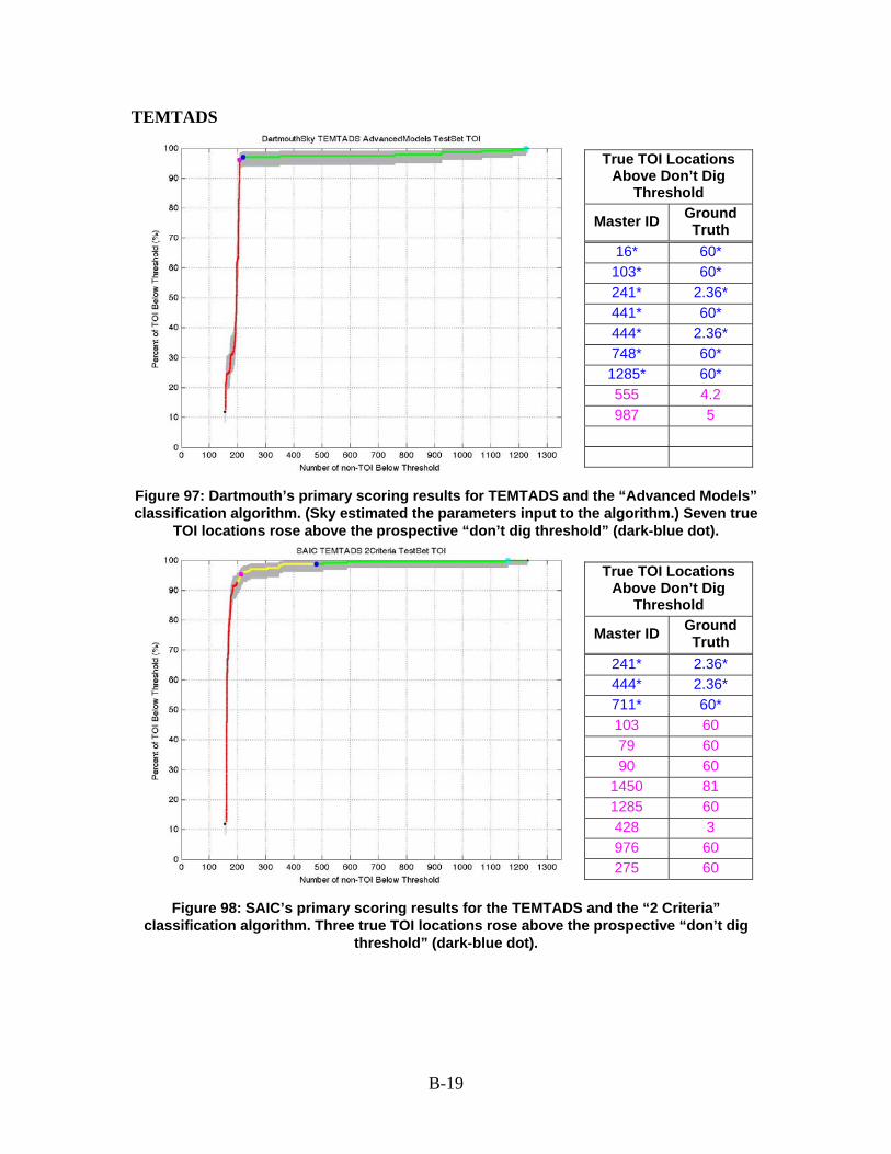
B-19

TEMTADS

True TOI Locations Above Don’t Dig

Threshold

Master ID Ground Truth

16* 60*

103* 60*

241* 2.36*

441* 60*

444* 2.36*

748* 60*

1285* 60*

555 4.2

987 5

Figure 97: Dartmouth’s primary scoring results for TEMTADS and the “Advanced Models” classification algorithm. (Sky estimated the parameters input to the algorithm.) Seven true

TOI locations rose above the prospective “don’t dig threshold” (dark-blue dot).

True TOI Locations Above Don’t Dig

Threshold

Master ID Ground Truth

241* 2.36*

444* 2.36*

711* 60*

103 60

79 60

90 60

1450 81

1285 60

428 3

976 60

275 60

Figure 98: SAIC’s primary scoring results for the TEMTADS and the “2 Criteria” classification algorithm. Three true TOI locations rose above the prospective “don’t dig

threshold” (dark-blue dot).

B-20

True TOI Locations Above Don’t Dig

Threshold

Master ID Ground Truth

241* 2.36*

711* 60*

444* 2.36*

16* 60*

249* 60*

372* 60*

65* 60*

103 60

90 60

79 60

1450 81

Figure 99: SAIC’s primary scoring results for the TEMTADS and the “3 Criteria” classification algorithm. Seven true TOI locations rose above the prospective “don’t dig

threshold” (dark-blue dot).

True TOI Locations Above Don’t Dig

Threshold

Master ID Ground Truth

1415* 4.2*

241* 2.36*

775* 60*

444* 2.36*

441* 60*

987* 5*

90 60

103 60

79 60

711 60

722 60

Figure 100: SAIC’s primary scoring results for the TEMTADS and the “Multisource - 3 Criteria” classification algorithm. Six true TOI locations rose above the prospective “don’t

dig threshold” (dark-blue dot).

B-21

True TOI Locations Above Don’t Dig

Threshold

Master ID Ground Truth

444* 2.36*

1415* 4.2*

241* 2.36*

1450* 81*

90* 60*

722* 60*

118* 4.2*

152* 4.2*

987* 5*

249* 60*

711* 60*

Figure 101: SAIC’s primary scoring results for the TEMTADS and the “Multisource - SVM” classification algorithm. Nineteen true TOI locations rose above the prospective “don’t dig

threshold” (dark-blue dot), the first 11 of which are listed above in blue.

True TOI Locations Above Don’t Dig

Threshold

Master ID Ground Truth

444* 2.36*

241* 2.36*

555* 4.2*

1450* 81*

21* 4.2*

850* 4.2*

1285* 60*

208* 4.2*

1386 81

711 60

722 60

Figure 102: SIG’s primary scoring results for the TEMTADS and the RVM supervised learning classification algorithm. Eight true TOI locations rose above the prospective

“don’t dig threshold” (dark-blue dot).

B-22

True TOI Locations Above Don’t Dig

Threshold

Master ID Ground Truth

444* 2.36*

1285* 60*

722 60

241 2.36

1450 81

1386 81

21 4.2

748 60

16 60

103 60

55 60

Figure 103: SIG’s primary scoring results for the TEMTADS and the PNBC semi-supervised learning classification algorithm. Two true TOI locations rose above the prospective “don’t

dig threshold” (dark-blue dot).

True TOI Locations Above Don’t Dig

Threshold

Master ID Ground Truth

241* 2.36*

1450* 81*

1285* 60*

410* 60*

107* 60*

103* 60*

444* 2.36*

748* 60*

122* 60*

22* 60*

275* 60*

Figure 104: SIG’s primary scoring results for the TEMTADS and the RVM supervised learning classification algorithm. The algorithm was optimized over the Active Learning Training Set and then applied to the complementary Active Learning Test Set. Fifty-two true TOI locations rose above the prospective “don’t dig threshold” (dark-blue dot), the

first 11 of which are listed above in blue.

B-23

True TOI Locations Above Don’t Dig

Threshold

Master ID Ground Truth

241* 2.36*

1450* 81*

208 4.2

987 5

103 60

55 60

107 60

444 2.36

122 60

1444 60

109 60

Figure 105: SIG’s primary scoring results for the TEMTADS and the RVM supervised learning classification algorithm. (Sky estimated the parameters input to the algorithms.) Two true TOI locations rose above the prospective “don’t dig threshold” (dark-blue dot).

True TOI Locations Above Don’t Dig

Threshold

Master ID Ground Truth

241* 2.36*

1450 81

55 60

444 2.36

987 5

208 4.2

1444 60

160 60

60 60

109 60

775 60

Figure 106: SIG’s primary scoring results for the TEMTADS and the PNBC semi-supervised learning classification algorithm. (Sky estimated the parameters input to the algorithms.) One true TOI location rose above the prospective “don’t dig threshold” (dark-blue dot).

B-24

True TOI Locations Above Don’t Dig

Threshold

Master ID Ground Truth

241* 2.36*

16* 60*

103* 60*

1285* 60*

314 60

365 4.2

444 2.36

441 60

249 60

711 60

443 60

Figure 107: Sky’s primary scoring results for the TEMTADS and the “Expert Opinion” classification algorithm. Four true TOI location rose above the prospective “don’t dig

threshold” (dark-blue dot).

True TOI Locations Above Don’t Dig

Threshold

Master ID Ground Truth

241* 2.36*

711* 60*

314 60

365 4.2

444 2.36

208 4.2

452 81

722 60

372 60

207 60

103 60

Figure 108: Sky’s primary scoring results for the TEMTADS and the “Library” classification algorithm. Two true TOI locations rose above the prospective “don’t dig

threshold” (dark-blue dot).

B-25

True TOI Locations Above Don’t Dig

Threshold

Master ID Ground Truth

241* 2.36*

103* 60*

16* 60*

314 60

365 4.2

444 2.36

79 60

90 60

443 60

60 60

72 60

Figure 109: Sky’s primary scoring results for the TEMTADS and the “Polarization Match” classification algorithm. Three true TOI locations rose above the prospective “don’t dig

threshold” (dark-blue dot).

True TOI Locations Above Don’t Dig

Threshold

Master ID Ground Truth

241* 2.36*

16* 60*

103* 60*

314 60

365 4.2

444 2.36

443 60

1285 60

441 60

60 60

241 2.36

Figure 110: Sky’s primary scoring results for the TEMTADS and the “Statistical Classifier” classification algorithm. Three true TOI locations rose above the prospective “don’t dig

threshold” (dark-blue dot).

B-26

MetalMapper

True TOI Locations Above Don’t Dig

Threshold

MM ID Ground Truth

737* 60*

254 60

292 37

852 60

1604 81

31 60

40 60

50 60

Figure 111: Dartmouth’s primary scoring results for the MetalMapper and the “Advanced Models” classification algorithm. (Sky estimated the parameters input to the algorithm.) One true TOI location rose above the prospective “don’t dig threshold” (dark-blue dot).

True TOI Locations Above Don’t Dig

Threshold

MM ID Ground Truth

1177* 60*

292* 37*

1718* 2.36*

737 60

493 60

2195 2.36

2149 60

368 60

852 60

Figure 112: Geometrics’ primary scoring results for the MetalMapper and the “ANN-LM-A” classification algorithm. Three true TOI locations rose above the prospective “don’t dig

threshold” (dark-blue dot).

B-27

True TOI Locations Above Don’t Dig

Threshold

MM ID Ground Truth

292* 37*

1718* 2.36*

1177* 60*

1771 60

886 5

493 60

737 60

988 81

595 60

1626 3

2149 60

Figure 113: Geometrics’ primary scoring results for the MetalMapper and the “ANN-TKLM” classification algorithm. Three true TOI locations rose above the prospective “don’t dig

threshold” (dark-blue dot).

True TOI Locations Above Don’t Dig

Threshold

MM ID Ground Truth

1177* 60*

737* 60*

680* 2.36*

493* 60*

852* 60*

1718 2.36

292 37

1626 3

2306 60

781 60

2410 60

Figure 114: SAIC’s primary scoring results for the MetalMapper and the “2 Criteria” classification algorithm. Five true TOI locations rose above the prospective “don’t dig

threshold” (dark-blue dot).

B-28

True TOI Locations Above Don’t Dig

Threshold

MM ID Ground Truth

1177* 60*

493* 60*

852* 60*

680* 2.36*

1718 2.36

292 37

737 60

1160 60

2104 2.36

163 2.36

1177 60

Figure 115: SAIC’s primary scoring results for the MetalMapper and the “3 Criteria” classification algorithm. Four true TOI locations rose above the prospective “don’t dig

threshold” (dark-blue dot).

True TOI Locations Above Don’t Dig

Threshold

MM ID Ground Truth

292* 37*

2420* 81*

1177* 60*

1718* 2.36*

746* 60*

737* 60*

771 81

1626 3

886 5

781 60

1754 81

Figure 116: SIG’s primary scoring results for the MetalMapper and the RVM supervised learning classification algorithm. Six true TOI locations rose above the prospective “don’t

dig threshold” (dark-blue dot).

B-29

True TOI Locations Above Don’t Dig

Threshold

MM ID Ground Truth

1718* 2.36*

1177* 60*

746* 60*

781* 60*

292* 37*

2420* 81*

529 60

499 60

Figure 117: SIG’s primary scoring results for the MetalMapper and the PNBC semi-supervised learning classification algorithm. Six true TOI locations rose above the

prospective “don’t dig threshold” (dark-blue dot).

True TOI Locations Above Don’t Dig

Threshold

MM ID Ground Truth

1718* 2.36*

292* 37*

1177* 60*

737 60

1771 60

781 60

746 60

1915 60

493 60

731 60

1718 2.36

Figure 118: Sky’s primary scoring results for the MetalMapper and the “Expert Opinion” classification algorithm. Three true TOI locations rose above the prospective “don’t dig

threshold” (dark-blue dot).

B-30

True TOI Locations Above Don’t Dig

Threshold

MM ID Ground Truth

1718* 2.36*

1177* 60*

1771* 60*

2420* 81*

371 60

595 60

564 2.36

410 60

Figure 119: Sky’s primary scoring results for the MetalMapper and the “Library” classification algorithm. Four true TOI locations rose above the prospective “don’t dig

threshold” (dark-blue dot).

True TOI Locations Above Don’t Dig

Threshold

MM ID Ground Truth

1718* 2.36*

292* 37*

1177 60

781 60

746 60

1915 60

493 60

731 60

Figure 120: Sky’s primary scoring results for the MetalMapper and the “Statistical Classifier” classification algorithm. Two true TOI locations rose above the prospective

“don’t dig threshold” (dark-blue dot).

B-31

BUD

True TOI Locations Above Don’t Dig

Threshold

Master ID Ground Truth

444* 2.36*

1285 60

1372 2.36

Figure 121: LBNL’s primary scoring results for the BUD and the “Empirical Likelihood Ratio” classification algorithm. Results were scored over only the sub-areas of the site

where the BUD collected data. One true TOI location rose above the prospective “don’t dig threshold” (dark-blue dot).

True TOI Locations Above Don’t Dig

Threshold

Master ID Ground Truth

241* 2.36*

Figure 122: LBNL’s primary scoring results for the BUD and the “Template Match” classification algorithm. Results were scored over only the sub-areas of the site where the BUD collected data. Rather than ordering the BUD cued locations into a ranked anomaly list, LBNL simply classified them as either “Likely TOI” or “Likely Non-TOI.” One true TOI

location was incorrectly classified as “Likely Non-TOI” (dark-blue dot). (The classifications were made after LBNL received ground truth for the Test Set.)

B-32

True TOI Locations Above Don’t Dig

Threshold

Master ID Ground Truth

241* 2.36*

1285* 60*

1372* 2.36*

Figure 123: SIG’s primary scoring results for the BUD and the RVM supervised learning classification algorithm. (LBNL estimated the parameters input to the algorithm.) Results were scored over only the sub-areas of the site where the BUD collected data. Three true

TOI locations rose above the prospective “don’t dig threshold” (dark-blue dot), all of which are listed in blue. (The ranked anomaly list was created after SIG received ground truth for

the Test Set.)

True TOI Locations Above Don’t Dig

Threshold

Master ID Ground Truth

241 2.36

1372 2.36

1285 60

Figure 124: SIG’s primary scoring results for the BUD and the PNBC semi-supervised learning classification algorithm. (LBNL estimated the parameters input to the algorithm.) Results were scored over only the sub-areas of the site where the BUD collected data. No true TOI locations rose above the prospective “don’t dig threshold” (dark-blue dot). (The

ranked anomaly list was created after SIG received ground truth for the Test Set.)

B-33

True TOI Locations Above Don’t Dig

Threshold

Master ID Ground Truth

241* 2.36*

444 2.36

1444 60

Figure 125: Sky’s primary scoring results for the BUD and the PNN classification algorithm. Results were scored over only the sub-areas of the site where the BUD

collected data. One true TOI location rose above the prospective “don’t dig threshold” (dark-blue dot). (The ranked anomaly list was created after Sky received the ground truth

for the Test Set.)

C-1

REFERENCES

[1] “2008 ESTCP UXO Classification Study, San Luis Obispo, CA,” ESTCP, September 2008.

[2] “Adaptive and Interactive Processing Techniques for Overlapping Signatures: Technical Summary Report,” AETC Inc., March 2006.

[3] “Draft Final Report: LGP Discrimination and Residual Risk Analysis: 2008-9 ESTCP UXO Classification Study, Camp Sibert and Camp San Luis Obispo,” ESTCP Project #MM-0811, SAIC and RML Technologies Inc.

[4] “EM61-Mk2 Cart Data Collection and Analysis: Former Camp San Luis Obispo,” NAEVA Geophysics Inc., April 2009.

[5] “EMI Array for Cued UXO Discrimination: Draft Data Collection Report: Former Camp San Luis Obispo,” ESTCP Project #MM-00601, SAIC, July 2009.

[6] “Draft Demonstration Data Report: Former Camp San Luis Obispo: Magnetometer and EM61 MkII Surveys,” ESTCP Project #MM-0744, Nova Research Inc., July 2009.

[7] “Feature Extraction and Classification of Magnetic and EMI Data: Camp San Luis Obispo,” ESTCP Project #MM-0504, Sky Research Inc., March 2010.

[8] “Final Site Inspections Report: Former Camp San Luis Obispo,” Parsons Inc., September 2007.

[9] “Former Camp San Luis Obispo: SAIC Final Report,” SAIC, March 2010.

[10] “Report of the Defense Science Board Task Force on Unexploded Ordnance,” Office of the Under Secretary of Defense for Acquisition, Technology, and Logistics, December 2003.

[11] “Slope Correction and Anomaly Memorandum: Former Camp San Luis Obispo,” Nova Research Inc., May 2009.

[12] Carin, L., et al., “2009 ESTCP UXO Discrimination Study, San Luis Obispo, CA,” ESTCP Project #MM-200501, Signals Innovations Group, April 2010.

[13] Cazares, S., et al., “The UXO Discrimination Study at the Former Camp Sibert,” IDA Document D-3572, Institute for Defense Analyses, January 2009.

[14] Gasperikova, E., “Technology Demonstration Plan Draft: ESTCP UXO Discrimination Study,” ESTCP Project #MM-0838, Lawrence Berkeley National Laboratory, January 2009.

[15] Macshassy, S., and Provost, F., “Confidence Bands for ROC Curves: Methods and Empirical Study, Proc. 1st Workshop on ROC Analysis in AI, 2004.

[16] May, M., and Tuley, M., “Interpreting Results from the Standardized UXO Test Sites,” IDA Document D-3280, Institute for Defense Analyses, January 2007.

[17] Nelson, H., et al., “ESTCP Pilot Program: Classification Approaches in Munitions Response: San Luis Obispo, California,” ESTCP, May 2010.

C-2

[18] Paski, A., “Memorandum: Description of Additional EM61 Cart Prioritized Dig Lists,” NAEVA Geophysics Inc., November 2009.

[19] Prouty, M., “Data Collection Report: MetalMapper System: Camp San Luis Obispo Discrimination Study,” ESTCP Project #MM-0603, Geometrics Inc., July 2009.

[20] Prouty, M., “Draft Demonstration Plan: Detection and Classification with the MetalMapper at the Former Camp San Luis Obispo,” ESTCP Project #MM-0603, Geometrics Inc., March 2009.

[21] Siegel, R., “MSEMS SLO Draft Data Report,” SAIC, August 2009.

[22] Tuley, M., et al., “UXO Classification Study: Blind Seed Plan at the Former Camp San Luis Obispo,” Institute for Defense Analyses, October 2008.

[23] Walker, A., “Memorandum: Classification of SLO EM61-MK2 Cart Targets,” U.S. Army Engineering and Support Center, Huntsville, January 2010.

[24] Walker, A., “Memorandum: Update to Classification of SLO EM61-MK2 Cart Targets,” U.S. Army Engineering and Support Center, Huntsville, January 2010.

D-1

ACRONYMS

EMI polarizability

EMI polarizability decay rate

BUD Berkeley UXO Discriminator

CEHNC Corps of Engineers – Huntsville Center

DGPS Differential Global Positioning System

EMI Electromagnetic induction

ESTCP Environmental Security Technology Certification Program

FN False negative

FP False positive

GLRT Generalized likelihood ratio test

GPS Global Positioning System

IDA Institute for Defense Analyses

IMU Inertial measurement unit

IVS Instrument Verification Strip

MSEMS Man-portable Simultaneous Magnetometer and Electromagnetic System

MTADS Multi-sensor Towed Array Detection System

N/A Not applicable

Pd Probability of detection

PNBC Parameterized neighborhood-based classification

PNN Probabilistic neural network

ROC Receiver operating characteristic

RTK Real time kinematic

RVM Relevance Vector Machine

SAIC Science Applications International Corporation

SERDP Strategic Environmental Research and Development Program

SIG Signals Innovations Group

SLO San Luis Obispo

SNR Signal-to-noise ratio

TEMTADS Time-domain Electromagnetic Multi-sensor Towed Array Detection System

TOI Target of interest

D-2

TP True positive

UXO Unexploded ordnance

REPORT DOCUMENTATION PAGE Form Approved

OMB No. 0704-0188 The public reporting burden for this collection of information is estimated to average 1 hour per response, including the time for reviewing instructions, searching existing data sources, gathering and maintaining the data needed, and completing and reviewing the collection of information. Send comments regarding this burden estimate or any other aspect of this collection of information, including suggestions for reducing the burden, to Department of Defense, Washington Headquarters Services, Directorate for Information Operations and Reports (0704-0188), 1215 Jefferson Davis Highway, Suite 1204, Arlington, VA 22202-4302. Respondents should be aware that notwithstanding any other provision of law, no person shall be subject to any penalty for failing to comply with a collection of information if it does not display a currently valid OMB control number.

PLEASE DO NOT RETURN YOUR FORM TO THE ABOVE ADDRESS. 1. REPORT DATE

September 2010 2. REPORT TYPE

Final 3. DATES COVERED (From–To)

May 2008 – January 2010 4. TITLE AND SUBTITLE

The UXO Classification Demonstration at

San Luis Obispo, CA

5a. CONTRACT NUMBER DASW01 04 C 0003

5b. GRANT NUMBER

5c. PROGRAM ELEMENT NUMBER

6. AUTHOR(S) Shelley Cazares Michael Tuley

5d. PROJECT NUMBER

5e. TASK NUMBER AM-2-1528

5f. WORK UNIT NUMBER

7. PERFORMING ORGANIZATION NAME(S) AND ADDRESS(ES) Institute for Defense Analyses 4850 Mark Center Drive Alexandria, VA 22311-1882

8. PERFORMING ORGANIZATION REPORT NUMBER

IDA Document D-4148 Log: H10-000937

9. SPONSORING / MONITORING AGENCY NAME(S) AND ADDRESS(ES)

Environmental Security Technology Certification Program 901 N. Stuart Street, Suite 303 Arlington, VA 22203

10. SPONSOR/MONITOR’S ACRONYM(S)

11. SPONSOR/MONITOR’S REPORT NUMBER(S)

12. DISTRIBUTION/AVAILABILITY STATEMENT Approved for public release; distribution is unlimited. (8 March 2011)

13. SUPPLEMENTARY NOTES

14. ABSTRACT Under a task titled “ESTCP/SERDP: Assessment of Traditional and Emerging Approaches to the Detection and

Identification of Surface and Buried Unexploded Ordnance,” the Institute for Defense Analyses (IDA) was assigned the responsibility to assist ESTCP in planning, executing, and scoring the classification demonstration carried out at San Luis Obispo, CA. IDA’s principal functions were to provide seed emplacement locations and burial procedures, create a master anomaly list, develop scoring protocols, and score demonstrators’ detection and classification results. This document provides a comprehensive final report describing the demonstration.

15. SUBJECT TERMS Unexploded Ordnance, classification, electromagnetic induction, magnetometer, receiver operating characteristics curves

16. SECURITY CLASSIFICATION OF: 17. LIMITATION OF

ABSTRACT

SAR

18. NUMBER OF

PAGES

148

19a. NAME OF RESPONSIBLE PERSONDr. Herbert Nelson

a. REPORT Uncl.

b. ABSTRACT Uncl.

c. THIS PAGE Uncl.

19b. TELEPHONE NUMBER (include area code)

703-696-8726

Standard Form 298 (Rev. 8-98) Prescribed by ANSI Std. Z39.18