The Utilization Premium ⋆ - Foti Grigoris

The Utilization Premium ?

Fotis Grigoris and Gill Segal

February 2021

Abstract

We study the implications of flexible capacity utilization for firms’ risk and invest-ment. First, we document that firms that underutilize their capital are riskier. Aninvestment strategy that longs (shorts) equities with low (high) utilization rates earns5% p.a. Utilization predicts excess returns beyond other production-based character-istics. We reconcile this novel utilization premium quantitatively using a productionmodel. Second, the model suggests that flexible utilization is important for matchingthe cross-sectional distribution of investment and stock prices jointly. A model with-out flexible utilization yields many counterfactuals: investment’s dispersion is too low,and its skewness bears the wrong sign. Flexible utilization addresses these momentsby making depreciation fluctuate endogenously. Overall, utilization tightens the linkbetween firms’ production and valuation.

JEL classification: G12, E23, E32

Keywords: Production, Capacity, Utilization, Productivity, Asset Pricing

?Grigoris: Kelley School of Business, Indiana University, Hodge Hall, Bloomington, IN 47405, U.S.A. (e-mail:[email protected]); Segal (corresponding author): Kenan-Flagler Business School, University of North Carolina atChapel Hill, McColl Building, Chapel Hill, NC 27599, U.S.A. (e-mail: [email protected]). Thispaper benefited from comments and suggestions by Max Croce, Ric Colacito, Winston Dou (discussant), Eric Ghy-sels, Erik Loualiche (discussant), Christian Lundblad, Jun Li (discussant), Dimitris Papanikolaou, Nick Roussanov,Jincheng Tong (discussant), Miao Ben Zhang (discussant), Harold Zhang, and seminars participants at the 2019MFA annual meeting, 2019 Northern Finance Association meeting, 2019 Fall UT Dallas Finance Conference, 2020RAPS Winter Conference, 2020 Australasian Finance & Banking Conference, and the University of North Carolinaat Chapel Hill. All errors are our own.

Capacity utilization measures the extent to which a business uses its production potential. Flex-

ible capacity utilization lets firms scale their production by choosing how much of their machinery

to operate. For instance, instead of decreasing production by selling machines, the firm can choose

to keep some machines idle. While existing studies in macroeconomics demonstrate the ability of

aggregate-level utilization to predict the business cycle, the extent to which granular-level (i.e., firm

or industry level) utilizations quantitatively affect risk and investment remains largely unexplored.

In this paper we examine this relationship both empirically and theoretically, and show that it

is not only sizable, but also bears important implications for reconciling the joint distribution of

cross-sectional real quantities and prices.

First, we show that lower utilization is associated with a substantially higher risk premium

in the cross-section of equities. Second, we construct a production economy that highlights the

role of flexible utilization for the intertemporal choice of capital. The model serves two goals:

(1) it explains the relation between utilization and risk premia quantitatively, and (2) it shows

that flexible utilization is crucial for production models with real options to target cross-sectional

investment moments alongside risk premia spreads. Namely, when utilization changes from fixed

to flexible, the dispersion and skewness of investment rates rise, as in the data. This increases the

dispersion of firms’ exposures to aggregate productivity. Thus, a model with flexible utilization

generates large cross-sectional variation in expected returns (e.g., a sizable value premium), while

relying on lower and fewer exogenous capital adjustment costs parameters. As such, the theoretical

merit of flexible utilization for macro-finance studies extends well-beyond reconciling the utilization

premium.

Empirically, we start by establishing two novel facts. Using capacity utilization data for a cross-

section of industries, we document that firms that belong to low capacity utilization industries earn

an average annual return that is 5.7% higher than the annual return earned by firms that belong to

high capacity utilization industries. We term this return spread the Utilization Premium. We then

show that there exists a monotonically decreasing relation between utilization rates and aggregate

productivity exposures: the low utilization portfolio has a higher aggregate productivity beta than

the high utilization portfolio, consistent with the premium. Moreover, we find that exposures to

aggregate productivity are time-varying, and depend negatively on the utilization rate.

While the baseline utilization premium is based on industry-level return data, the premium is not

simply capturing cross-sectoral heterogeneity. We show this in four main ways. First, the spread

exists within economic sectors. For instance, an economically large utilization spread emerges

among durable manufacturers only. Moreover, utilization negatively forecasts future excess returns

in predictive regressions that control for sectoral fixed effects. Second, we show the utilization

1

spread persists when we form portfolios using the growth rate of utilization, thereby eliminating

any industry-specific fixed effects in utilization’s level. Third, we construct proxies for firm-level

utilization rates using Compustat data. The utilization premium remains positive when sorting

firms into portfolios based on these novel firm-level utilization proxies. Lastly, through the lens

of our model, we show that ex-ante heterogeneity in depreciation or adjustment cost parameters

between firms contributes only marginally to the utilization premium.

The utilization premium is robust feature of the data, and distinct from related production-

based margins. Fama and MacBeth (1973) regressions and double sort analyses show that utiliza-

tion’s explanatory power for risk premia is incremental to key characteristics, such as investment

and hiring, book-to-market, productivity, financing frictions, and intangible (organization) capital.

While the utilization premium does not represent a source of risk that is separate from aggregate

productivity, utilization bears incremental predictive power for expected returns through its effect

on firms’ conditional productivity risk exposures.

To rationalize our findings and explore the quantitative gains of variable utilization for macro-

finance, we incorporate the realistic feature of utilization decision into a quantitative production

model. Importantly, the calibration of the model does not directly target the utilization spread.

Yet, the framework matches multiple untargeted moments of real quantities and asset prices. The

model yields two general implications.

The first implication relates to the utilization spread. The model is able to quantitative replicate

the novel facts. In particular, the magnitude of the utilization premium in the model matches the

data. As such, the model-implied utilization premium serves as a theoretical prediction, providing

support to the empirical evidence. The intuition for the spread is summarized below.

In the model, firms extend their production capacity by buying capital and decrease it by

selling machines in the secondary market for capital. This market involves frictions. Specifically,

the model features a fixed cost for capital disinvestment, making selling machines a real option.

The key ingredient is a variable capacity utilization rate that controls the extent to which installed

capital is utilized. Increasing the utilization rate is costly, as it makes capital depreciate faster.1

In an economy in which the capacity utilization rate is fixed, firms can only reduce the cyclicality

of their payouts via investment decisions. If adjusting capital is costly, then the risk of each firm is

determined entirely by the interaction between aggregate productivity and these capital adjustment

costs.2 With flexible utilization, firms have an additional mechanism to decrease the cyclicality of

1We consider an extension of our model in which the depreciation rate of a firm depends not only on its utilizationchoice, but also on exogenous depreciation shocks. Allowing for exogenous shocks to depreciation induces only asmall quantitative effect on the results, highlighting the importance of endogenous utilization.

2Firms that disinvest (invest) the most in low (high) aggregate productivity states are required to pay large capitaladjustments costs. Consequently, since these firms are unable to fully absorb the impact of productivity shocks on

2

productivity shocks on payouts.

To illustrate how utilization is tied to firms’ risk, consider an economy featuring convex and

symmetric capital adjustment costs. A firm operating in a low productivity state has the incentive

to reduce its capital, thereby exposing itself to potentially large adjustment costs. Simultaneously,

the firm has an incentive to lower its utilization rate. By lowering utilization the firm reduces its

capital depreciation rate. This reduced depreciation not only conserves capital for future states

that are more productive, but also reduces the adjustment cost of downsizing.3 By similar logic,

increasing utilization in good states reduces the adjustment cost for expanding capital by increasing

depreciation. Thus, utilization and investment comove positively. This implies that both very high

and very low utilization firms have high exposures to aggregate productivity. Both extremes reflect

firms that incur high risk by desiring to modify their capital stock to a large extent under adjustment

costs. Simultaneously altering utilization partially hedges their (dis)investment policies.

Two mechanisms break the symmetry between high and low utilization firms. First, with a

positive fixed adjustment cost disinvestment becomes a costly real option. Firms with moderately

low levels of productivity substitute disinvestment by lowering utilization. Instead of selling capital,

firms temporarily downscale by under-utilizing installed machines. As the friction in the market for

selling capital is higher for these firms, they are riskier. Second, the model features a countercylical

market price of risk (motivated by countercylical volatility). Thus, firms’ whose valuations covary

more with economic conditions during bad states command a larger risk premium. Since low

utilization firms have higher productivity betas in bad states, they earn higher expected returns.

The second general implication of the model is that flexible utilization plays a pivotal role for

simultaneously matching investment and asset-pricing moments in the presence of real investment

options. In the model, whenever utilization is fixed, the cross-sectional dispersion and skewness of

investment are less than half of their empirical magnitudes. The time-series skewness of firm-level

investment is negative, whereas it is positive in the data. This happens because disinvestment

in the model is a costly real option. During moderate economic slowdowns, firms “wait and see”

if productivity will improve before opting to sell capital. Under fixed utilization, these firms do

not alter their capital stocks and set their investment rates equal to the (constant) depreciation

rate instead. Because a mass of waiting firms are then lumped around the center of investment’s

distribution, the cross-section of investment rates is compressed, and features low dispersion. If

productivity is persistently negative, these waiting firms pass a tipping point in which they are

their payouts, these firms are risky.3In other words, lower utilization implies that the current depreciation, δt, falls. With quadratic adjustment

frictions over net investment, the adjustment cost is proportional to the distance between it, the investment rate,and δt. As δt drops whenever it drops, the adjustment cost falls.

3

overly burdened with unproductive capital, and disinvest sharply. These disinvestment jumps create

the counterfactual negative sign for the time-series skewness of investment. As the distribution of

investment rates is too compressed, firms’ risk exposures to aggregate productivity do not feature

enough heterogeneity, which shrinks investment-related spreads such as the value premium.

Introducing flexible utilization to the model addresses the former misses. When utilization is

flexible, firms can respond to moderate drops in productivity by utilizing less capital. This causes

depreciation to fall, and reduces the investment required to preserve the current capital stock. Since

the natural (or preservation) rate of investment in this economy is time-varying, even firms that

“wait and see” have to keep altering their investment rates to preserve their existing capital. Thus,

the long periods of constant investment rates are eliminated. Time-varying depreciation rates that

are (ex-post) heterogeneous between firms increase the cross-sectional dispersion of investment.

This is because waiting firms are no longer massed at the same investment rate. Moreover, since

firms utilize their machines more intensively in good times, depreciation increases in these peri-

ods. Larger investments are needed to expand capital, causing the time-series and cross-sectional

skewness of investment to rise, turn positive, and match the data. Lastly, greater dispersion in in-

vestment suggest a larger dispersion in firms’ risk exposures, which boosts cross-sectional spreads.

The problem of matching moments under fixed utilization is not alleviated by recalibrating

the model. For instance, the diminished value premium in the model with fixed utilization can be

raised by increasing the convex capital adjustment costs. However, the adjustment costs required to

match the value premium with fixed utilization are 100% higher than those with flexible utilization.

This alternative calibration also has counterfactual implications for investment’s dispersion. We

also augment a fixed-utilization model with more complex adjustment costs, which require extra

model parameters. We find that while the model fit is improved, it still fails to fully reconcile the

data. As such, utilization “saves” the degree of exogenous parameters needed to explain the data.

Lastly, our model suggests that firms’ depreciation and utilization rates should comove pos-

itively. We confirm this prediction in the data. We demonstrate that utilization is useful for

measuring depreciation rates. Recent macro-finance studies suggest that BEA- and Compustat-

based depreciations exhibit a low correlation, leading to different distributions of gross investment

rates. We show that utilization shrinks the wedge between BEA- and Compustat-implied deprecia-

tion rates. While the correlation between the two is only 3%, this correlation increases to 14% when

accounting for utilization fluctuations. Related, we augment our model with stochastic depreciation

shocks, thereby reducing the model-implied correlation between utilization and depreciation rates,

and show this additional shock has only a minor effect on the utilization premium.

Taken together, our empirical and theoretical results emphasize the economically important

4

relation between capacity utilization, investment, and risk premia, and tighten the connection

between firms’ production dynamics and their valuations.

The paper proceeds as follows. Section 1 reviews the related literature. Section 2 establishes the

novel empirical facts. Section 3 a model with flexible utilization rates to rationalize these findings.

Section 4 examines the relation between utilization and risk premia through the lens of the model.

Section 5 explores the theoretical implications of flexible utilization for investment dynamics and

adjustment costs. Section 6 provides concluding remarks.

1 Related literature

The paper contributes to the literatures on the role of capacity utilization in RBC models,

costly reversibility, and production-based asset pricing.

Our paper is tied to studies that examine the effects of time-varying capacity utilization in the

macroeconomic literature. As a leading indicator, aggregate utilization data is studied extensively

in relation to business cycle fluctuations. For instance, prior studies show how variable utilization

is useful for matching macroeconomic growth dynamics to the data (e.g., Greenwood, Hercowitz,

and Huffman (1988), and Jaimovich and Rebelo (2009)). Additionally, Burnside and Eichenbaum

(1996) show that variable utilization rates can propagate shocks over the business cycle, and amplify

the impact of technology shocks. The macroeconomic literature utilizes several empirical proxies for

utilization. Burnside, Eichenbaum, and Rebelo (1995) use electricity usage, while Basu, Fernald,

and Kimball (2006) use hours per worker to proxy for all unobserved intensive margins. Similar to

our empirical approach, Comin and Gertler (2006) use the FRB’s measure of capacity utilization

to study business cycle fluctuations over the medium-term.

In contrast to the macroeconomic literature, the relation between capacity utilization and asset

prices has received considerably less attention. This is despite the fact that capacity utilization is

conceptually related to firm-level production decisions, and despite the fact that the FRB regularly

reports granular data on the cross-section of utilization rates for various manufacturing and mining

industries, and utilities.4 Of the small set of papers that also study capacity utilization in the

context of asset pricing, most focus on aggregate asset-pricing moments. For instance, Garlappi

and Song (2017) include capacity utilization in a production-based asset pricing model and show

that varying utilization is important for the market price of risk of investment-specific technology

(IST) shocks. Da, Huang, and Yun (2017) use industrial electricity usage as a proxy for utilization

and find that higher electricity usage in the current period predicts lower stock market returns in

4While the U.S. manufacturing sector is of modest size, the sector still influences the macroeconomy to a largedegree (Andreou, Gagliardini, Ghysels, and Rubin, 2019). Consequently, capacity utilization figures are routinelyanalyzed by both the Federal Reserve Bank (FRB) and other market participants.

5

the future. This latter result is broadly consistent with our utilization premium, but pertains to

the time-series of market returns rather than the cross-section of equities that we study.

The model in Cooper, Wu, and Gerard (2005) focuses on explaining the value premium and also

includes capacity utilization. Although the authors find a qualitatively negative relation between

utilization and industry-level stock returns using OLS regressions, we emphasize the quantitative

relation between utilization to risk. We do this both theoretically, via a calibrated model, and em-

pirically, by establishing a novel spread. The utilization spread is distinct from the value premium,

and a host of other production-based characteristics. Our analysis also illustrates the importance

of flexible utilization for the joint distribution of investment rates and prices.

The notion of costly reversibility – the assumption that firms face higher costs to contract

rather than expand their capital stocks – continues to influence research in macroeconomics and

finance.5 In macroeconomics, recent studies such as Bloom (2009) and Bloom, Floetotto, Jaimovich,

Saporta-Eksten, and Terry (2018) combine costly reversibility and uncertainty shocks to explain

the dynamics of real quantities over the business cycle. In finance, costly reversibility has become

standard in many models rationalizing patterns in expected returns.

The studies of Zhang (2005), Carlson, Fisher, and Giammarino (2004) and Cooper (2006),

among others, explain the value premium and other cross-sectional spreads by assuming that capi-

tal is partially irreversible. Recent literature considers whether these canonical models can produce

realistic distributions of investment rates and risk premia jointly. While Clementi and Palazzo

(2019) present evidence that investment may not be as irreversible as these models suggest, Bai,

Li, Xue, and Zhang (2019) show that few firms disinvest capital, which supports the degree of irre-

versibility. The two studies differ in their measurement of gross investment rates.6 The importance

of utilization for jointly matching investment and prices extends beyond these two studies, as we

consider the additional frictions generated by costly real investment options. In the presence of

real options, flexible utilization is key for producing a realistic distribution of investment rates and

sizable risk premia. This conclusion is not driven by how gross investment is measured, but by

the inherent properties of the model. Our results indicate that real options (particularly those to

disinvest) are quantitatively important for (i) matching the magnitude of the utilization premium,

(ii) producing a realistic correlation between utilization and investment rates, and (iii) capturing

the negative impact of uncertainty shocks on investment as shown in Bloom (2009).

More broadly, our paper is related to asset-pricing studies that connect production economies to

5While the literature on costly reversibility is voluminous, some key studies include Dixit and Pindyck (1994),Abel and Eberly (1996), and Cooper and Haltiwanger (2006).

6Specifically, in Clementi and Palazzo (2019) gross investment rates are measured using industry-level depreciationrates from the Bureau of Economic Analysis. In Bai et al. (2019) gross investment rates are measured using firm-leveldepreciation expenses from Compustat.

6

expected returns (e.g., Belo and Lin (2012), Jones and Tuzel (2013),Belo, Lin, and Vitorino (2014b),

Kuehn and Schmid (2014), Ai and Kiku (2016), Belo, Li, Lin, and Zhao (2017), Kilic (2017), Tuzel

and Zhang (2017), Ai, Li, Li, and Schlag (2019), Dou, Ji, Reibstein, and Wu (2019), Loualiche et al.

(2019)). The relation between utilization and asset prices is of particular interest to this growing

literature that examines the joint dynamics of firm-level investment and risk premium.7

Prior studies in this literature include Belo, Lin, and Bazdresch (2014a), who study the impact

of labor market frictions on asset prices and find that firms with low hiring rates earn high returns.

We show empirically that hiring rates are indistinguishable between low and high utilization indus-

tries. Likewise, neither differences in intangible capital (e.g., Eisfeldt and Papanikolaou (2013)) nor

financing costs (e.g., Belo, Lin, and Yang (2018)) explain the utilization premium. Imrohoroglu and

Tuzel (2014) examine firm-level total factor productivity (TFP), and theoretically and empirically

show that low TFP firms earn a significant productivity premium. This is important for our study

because TFP and capacity utilization are linked by the fact that TFP can be decomposed into

three distinct components: utilization, markups, and technology. While utilization is a component

of TFP, we show empirically that most of the productivity premium stems from the technology and

markup components of TFP. That is, controlling for capacity utilization, the productivity premium

persists. Conversely, the utilization spread also persists after controlling for TFP.

Recently, Aretz and Pope (2018) estimate firm-level capacity overhang, or the difference between

a firm’s installed and optimal capital stock, and show that overhang has sizable implications for

cross-sectional risk premia. Although capacity utilization and overhang are conceptually similar,

we show that these margins result in theoretically and empirically distinct spreads. In particular,

both portfolio double sorts and Fama and MacBeth (1973) regressions show that the utilization

spread survives controlling for overhang, and vice versa.

In all, we contribute to the production-based asset pricing literature by focusing on the utiliza-

tion rate of productive units. We demonstrate that capacity utilization is an important determinant

of expected returns, and interacts with firms’ investment rates.

2 Empirical evidence

2.1 Data

Capacity utilization. We obtain industry-level utilization data from the FRB’s monthly

report on Industrial Production and Capacity Utilization (report G.17) that releases publicly avail-

able estimates of capacity utilization for a cross-section of industries that cover the manufacturing

7Similarly, Ai, Kiku, Li, and Tong (2018) examine firm-level outcomes, such as investment and dividends, in amodel featuring production and dynamic contracting, while Kogan, Li, and Zhang (2019) provide a production-basedexplanation for the investment and profitability premia.

7

and mining sectors, as well as utilities. The FRB uses this data to quantify how effectively different

industries are utilizing factors of production and to assess inflationary pressures (e.g., Corrado and

Mattey (1997)). A major advantage of this FRB data is that it provides a measure of utilization

that is available at a much higher frequency than estimates elicited from low-frequency accounting

data. The capacity utilization rate (CUi,t) of industry i at time t is given by:

CUi,t =IPi,t

Capacityi,t. (1)

Here, IPi,t is the actual output of the industry, measured by seasonally-adjusted industrial produc-

tion, and Capacityi,t is the FRB’s estimate of the industry’s sustainable maximal output at time t.

The capacity estimate for most industries is derived from the Quarterly Survey of Plant Capacity

Utilization conducted by the U.S. Census Bureau.

Our benchmark cross-section encompasses 45 industries, featuring a mix of durable manu-

facturers (18 industries), nondurable manufacturers (17 industries), and mining and utilities (10

industries).8 The time period of our benchmark analysis ranges from January 1967 to December

2015.9 The average utilization rate across all industries is roughly 80%. The unconditional mo-

ments of the mean, variance and autocorrelation of the utilization rate are similar across different

sectors. However, the relative ranking of industries in terms of utilization rates varies substantially

over time. We provide further details on the sample composition, including summary statistics, in

Section OA.2 of the Online Appendix.

Returns data. Monthly stock return data are taken from CRSP, and accounting data are taken

from the CRSP/Compustat Merged Fundamentals Annual file. We obtain returns for portfolios

sorted on key characteristics, such as size and book-to-market, as well as asset pricing factors related

to the Fama and French (1993, 2015) three- and five-factor models, and the Carhart (1997) four-

factor model, from the data library of Kenneth French. Data related to the Hou, Xue, and Zhang

(2015) q-factor model are provided by Lu Zhang and firm-level TFP data are from the website of

Selale Tuzel.10 Variable definitions are provided in Section OA.1 of the Online Appendix.

8While the FRB’s utilization data covers mostly manufacturing industries, we stress that: (1) the sector playsan important economic role in the aggregate economy. These are the industries underlying the aggregate industrialproduction index and they are key for long-term growth. Recent work by Andreou et al. (2019) shows that althoughthe manufacturing sector has diminished over time, the sector explains about 61% of the total GDP growth. Thus,our sample encompasses an important segment of the economy; (2) the sample of industries available by the FRBcorresponds mainly to good producers who utilize capital, and thus, ensures that the link between the productionmodel in Section 3 and the data is tight.

9The start date is based on the availability of capacity utilization data by the FRB. The end date reflects the timeat which the empirical work on this study commenced. It is worth noting that Table OA.3.5 in the Online Appendixshows that our results are strengthened in the second half of the sample period.

10We thank Kenneth French, Lu Zhang, and Selale Tuzel for making this data available to us.

8

2.2 Portfolio formation

To examine the relation between capacity utilization and stock returns in the data, we form

portfolios by sorting the cross-section of industries on the basis of each industry’s utilization rate.

Specifically, at the end of each June from 1967 to 2015 we sort industries into portfolios based on

their level of utilization in March of the same year. The three month lag between the release of

March utilization data and the June sort date ensures that this strategy is tradeable, as all data

used to form portfolios are publicly available by the portfolio formation dates.11 Each portfolio

is then held from July of year t to the end of June of year t + 1, at which time all portfolios are

rebalanced. Annual rebalancing allows us to capture conditional variation in utilization rates.

We form three portfolios on each June sorting date. The low (high) capacity utilization portfolio

includes all industries whose utilization rates are at or below (above) the 10th (90th) percentile of

the cross-sectional distribution of FRB industries’ utilization rates in March of the same year. The

medium utilization portfolio includes the remaining industries with utilization rates between these

breakpoints. We focus on these breakpoints to increase the power of our asset-pricing tests. This

is useful because our ability to detect a relation between utilization and future stock returns is

already limited by the cross-section of industries for which the FRB reports utilization data. It is

worth stressing, however, that since each portfolio contains multiple industries, each of which is

comprised of many firms, this choice of breakpoints produces three well-diversified portfolios. We

discuss the composition of the portfolios and their characteristics in Section 2.5. 12

2.3 Fact I: Utilization portfolios and expected returns

Table 1 reports the annual value- and equal-weighted returns of portfolios sorted on capacity

utilization using the procedure described above. We document an economically and statistically

significant spread between returns of the low and high utilization portfolios. We define the Uti-

lization Premium as the average return differential between the low and high utilization portfolios.

The table also shows that portfolio returns are monotonically decreasing in the average rate of

capacity utilization.

Specifically, the portfolio of industries that utilize a low amount of their productive capacity

earns a value-weighted (equal-weighted) average return of 13.64% (10.62%) per annum, whereas

the portfolio of industries that utilize a large degree of their capacity earns a value-weighted (equal-

11A three month lag between the portfolio formation month and the month in which utilization rates are measuredis conservative since the utilization data for month t are released approximately 15 days into month t+1. Since 1967,March utilization rates have been publicly available by April 17th at the latest.

12Table OA.3.18 in the Online Appendix reports the portfolio transition matrix. The matrix show that the probabil-ity of transitions out of the extreme portfolios are relatively frequent (about 25%). This demonstrates the importanceof the conditional portfolio rebalancing procedure, and the fact that industries change in their relative utilizationranking over time.

9

weighted) average return of return of 7.96% (5.18%) per annum. The value- and equal-weighted

spreads between the returns of the extreme utilization portfolios are 5.67% and 5.44% per annum,

respectively. Each spread is significant at the 5% level.13

Robustness. In Section OA.3.1 of the Online Appendix we show that the utilization spread is

robust to numerous methodological variations to the portfolio formation procedure. For instance,

Table OA.3.4 shows that assigning industries to quintiles, or three portfolios based on the 30th and

70th percentiles of the cross-sectional distribution of utilization rates, results in capacity utilization

spreads that are close to 5% p.a. and statistically significant. By and large, the portfolio returns

monotonically decrease in utilization. In addition, Table OA.3.5 shows that the magnitude of the

utilization premium rises to over 9% p.a. in the most recent half of the sample period. The spread

is also robust to other sorting frequencies, and to variations in the sample of industries.

Importantly, while the baseline utilization premium is based on industry-level data, we em-

phasize that the premium is not driven by ex-ante sectoral heterogeneity. For example, using the

growth rate of utilization as a sorting measure eliminates industry fixed effects in utilization’s level,

and still yields a sizable utilization-growth spread. We present rigorous evidence in Section 2.7 to

show that the utilization premium exists within economic sectors.

2.4 Fact II: Utilization portfolios and productivity exposures

Fixed exposures. We check whether the monotonic pattern between utilization rates and

expected return is a result of differential exposures to fundamental macroeconomic risk, as captured

by aggregate productivity betas. We consider the following projection

Retei,t = β0,i + β1,iAgg-Prodt + εi,t, (2)

where Retei,t is the value-weighted excess return of the portfolio i, Agg-Prodt is a proxy for aggregate

productivity, and β1,i captures the exposure of portfolio i to aggregate productivity. To implement

this analysis we consider three different proxies for aggregate productivity: the market return,

utilization-adjusted TFP growth from Fernald (2012), and labor productivity from the Bureau

of Labor Statistics (BLS). As the latter two proxies are only available quarterly, we aggregate

monthly returns to the quarterly frequency when estimating equation (2). Note that when we

proxy aggregate productivity using excess market returns, β0 corresponds to the CAPM alpha.

Table 2 reports the results. The exposure of the low utilization portfolio to aggregate produc-

tivity is higher the exposure of the high utilization portfolio, regardless of the productivity proxy.

Importantly, the differences in the productivity betas of the low and high utilization portfolios are

also statistically significant at roughly the 5% level or better. For instance, when measuring aggre-

13The Sharpe ratio of the value-weighted (equal-weighted) spread is 0.32 (0.35). This is comparable to the Sharperatio earned by investing in the value premium over the same period.

10

gate productivity using excess market returns, the difference in productivity betas is statistically

significant at better than the 1% level.

The table also shows that the intercepts from projecting the utilization spread on each pro-

ductivity proxy are generally insignificant. In particular, the CAPM alpha is insignificant at the

5% level (t-statistic = 1.78).14 Motivated by this evidence, along with the discussion below, our

model in Section 3 features a single source of risk: aggregate productivity. Exposures to this factor

endogenously vary with firms’ choice of utilization rates.

Time-varying exposures. A marginally significant CAPM alpha can arise due to time-

varying exposures to aggregate productivity, rather than an unaccounted risk factor. We verify

this conjecture in Online Appendix Section OA.3.2. We show that a conditional single-factor

model fully absorbs the utilization premium. We also establish a relation between time-varying

exposures and utilization rates. Three key findings are summarized below.

First, we follow the methodology of Lewellen and Nagel (2006), and show that the conditional

CAPM explains the utilization spread. The analysis is based on the average of alphas from rolling

window regressions of 12 months each. The results are reported in Table OA.3.8 of the Online

Appendix. The CAPM alpha of the utilization premium drops from 4.3% per annum (t-statistic of

1.78) under the unconditional case in Table 2, to 3.4% per annum (t-statistic of 1.34).

Second, to complement the evidence above, we augment projection (2) with a quadratic term

of aggregate productivity. This specification allows the relation between portfolio returns and pro-

ductivity to feature non-linearity – as in the case of time-varying risk exposures. We combine the

slope coefficient on the linear and quadratic terms of productivity to construct portfolios’ total

risk exposure. The results, given in Table OA.3.9, show that when this non-linearity is accounted

for, aggregate productivity exposures fully reconcile the utilization premium. The premium’s ex-

posure to aggregate productivity (linear + quadratic term) is statistically significant. Likewise, the

intercept drops to only 1.28% per annum (t-statistic of 0.41).

Third, we show that conditional market risk exposures depend negatively on utilization rates

in the cross-section of industries. We use a rolling window projection to estimate the time-varying

betas of each industry to the market excess return at the monthly frequency. We then run a panel

regression of conditional CAPM betas projected on utilization rates, controlling for industry and

time fixed effects. The results are shown in Online Appendix Table OA.3.10. The slope coefficient

on the utilization rate is negative and significant. This result is materially unchanged by controlling

14β0 can be interpreted as test of the CAPM only when we proxy for aggregate productivity using the marketreturn, but it is not restricted to zero under the null of CAPM when using TFP or labor productivity, as these arenon-tradable factors. Nonetheless, the fact that β0 is insignificant in these two cases complements the CAPM alpha,and emphasizes that statistically, the premium is absorbed by variations in productivity. Moreover, for all proxiesused, β1,i is still informative about the degree to which utilization is related to aggregate productivity exposure.

11

for other variables available at the monthly frequency, including size and idiosyncratic volatility.

Robustness. We verify that similar results hold for quintile utilization portfolios in Table

OA.3.11. By and large, in both the linear and non-linear model cases, the exposure to aggregate

productivity falls with the utilization rate, and the intercept of the non-linear model is insignificant.

2.5 Capacity utilization portfolios: Characteristics

Portfolio constituents. Panel A of Table 3 reports the average number of firms and industries

that constitute each utilization portfolio. By construction, the high and low utilization portfolios

each contain approximately 10% of the 45 industries in our sample. Although the number of

industries falling into these extreme portfolios is small, these industries are comprised of roughly

960 firms. This means that the low and high utilization portfolios collectively contain about 18%

of all firms in our merged CRSP-Compustat sample, and the extreme portfolios are well diversified.

Panel A also shows that the average utilization rate is, by construction, monotonically increasing

from the low to the high utilization portfolio.

To shed light on the industries underlying each portfolio, Table 4 reports the five industries

that populate the extreme utilization portfolios most often. For each industry, the table also

reports the sector to which the industry belongs, and the proportion of years the industry is sorted

into the portfolio. The key takeaway from this table is that there is a large degree of sectoral

variation associated with the industries that populate these portfolios. Panel A shows that leather

producers, aerospace manufacturers, and industries that provide supporting services to miners

frequently reside in the low utilization portfolio. Panel B shows that the high utilization portfolio

often contains mining industries, utilities, and nondurable manufactures.15 These results provide

suggestive evidence that the utilization premium is not driven by any one sector in particular.

Section 2.7.1 provides more rigorous evidence that the utilization spread is mostly a within-sector,

rather than a cross-sector phenomenon.

Portfolio characteristics. Panel B of Table 3 reports the average industry-level characteris-

tics of each capacity utilization portfolio. There is no statistically significant difference between the

low and high portfolios in terms of size, probability, as measured by either ROA or gross profitabil-

ity. Moreover, there are no differences in asset growth or inventory growth rates between the low

and high portfolios. Consistent with the fact that TFP and the hiring rate are positively correlated

with capacity utilization (see Table OA.2.3 of the Online Appendix), the low portfolio has both

lower industry-level TFP and hiring rates than the high portfolio. However, these differences are

small and statistically insignificant. Furthermore, neither external financing frictions, as measured

15While oil extraction appears quite frequently in the high utilization portfolio, we demonstrate in Table 6 andSection 2.7.1 that the utilization premium is positive and significant with the exclusion of the entire mining sector.

12

by leverage, debt growth, and equity issuance rates (e.g., Belo et al. (2018)), nor intangible capital,

as measured by R&D/ME or organizational capital (e.g., Lin (2012) and Eisfeldt and Papanikolaou

(2013)), differ significantly between low and high utilization firms. The only three characteristics

that are significantly different between the two extreme portfolios are the book-to-market ratios,

investment rates, and idiosyncratic return volatilities (IVOL).

The latter difference in IVOL cannot account for the capacity utilization premium, as Ang,

Hodrick, Xing, and Zhang (2006) show that high IVOL firms earn low expected returns, but low

utilization firms have higher IVOL. However, the former differences raise a concerns that since

low (high) capacity utilization industries also tend to be value (growth) industries with low (high)

investment rates, the utilization spread may be driven by the value or the investment premium.

Each of these potentially confounding effects are well-established in the context of the asset pricing

literature. For instance, Fama and French (1993) demonstrate the ability of book-to-market to

predict future stock returns, while Titman, Wei, and Xie (2004) show that low investment rates

are associated with high future returns.

To establish a degree of independence between the utilization spread and the value and invest-

ment premia, the next section conducts a Fama and MacBeth (1973) analysis. We show that the

relation between utilization and risk premia remains negative, economically large, and statistically

significant after controlling for book-to-market, investment, and a host of other production-based

characteristics.

2.6 Fama-MacBeth and double-sort analyses

Firm-level regressions. We perform firm-level Fama and MacBeth (1973) regressions and

show that capacity utilization has predictive power for risk premia that is incremental to the effects

of value, investment, and multiple other investment-related characteristics. These regressions are

implemented as follows. In each year t we run a cross-sectional regression in which the dependent

variable is a firm’s annual excess return from July in year t to June in year t+1, and the independent

variables are a vector of the firm’s characteristics, Xt, measured at the end of June in year t. The

cross-sectional regression specification is:

Ri,t→t+1 = β0,t + β′tXi,t + εi,t→t+1 ∀t ∈ {1967, . . . , 2014}. (3)

The characteristics we consider are capacity utilization, TFP, hiring, investment over physical

capital, capacity overhang, organization capital, the natural logarithms of size and book-to-market,

and the lagged annual return. A utilization rate is assigned to each firm following the procedure

described in Section OA.3.3 of the Online Appendix, and each control variable is divided by its

unconditional standard deviation to aid comparisons between regressions. After running these

cross-sectional regressions we compute the time-series average of each estimated slope coefficient to

13

assess the relation between a given characteristic and future stock returns, while holding all other

characteristics constant. The results are reported in Table 5.16

Columns 1 to 9 of Table 5 include each characteristic in a univariate regression. The average

loading of utilization is negative and statistically significant at the 5% level. The loadings on TFP,

hiring and investment rates, capacity overhang, and size are also negative and significant, while

the loading on book-to-market and organizational capital-to-assets is positive and significant. The

relation between lagged annual returns and future returns is statistically insignificant, indicating

that returns at the annual horizon have low autocorrelation. The signs of these variables are

consistent with the documented spreads associated with each characteristic of interest.17

Columns 10 to 16 show that the coefficient on utilization remains negative and significant at the

5% level when we include other investment-related characteristics in the regressions. Furthermore,

each of the extra characteristics we consider also remains negative and significant. This provides

additional evidence that the relation between utilization and stock returns is somewhat orthogonal

to the known relations between returns and each of TFP, hiring, investment, and capacity overhang.

Finally, Column 17 augments the regressors in Column 16 with organizational capital, size,

book-to-market, and past returns, and considers a regression featuring all eight characteristics

simultaneously. Column 18 also features all characteristics, and also include sector fixed effects.18

These fixed effects account for potential sectoral heterogeneity in the relation between utilization

and risk premia. In both columns, the loading on utilization remains negative and significant at

the 5% level. In particular, the result in Column 18 complements the extensive tests presented

next in Section 2.7, in support of the fact that the utilization premium is not driven by cross-

sectoral effects. Compared to Column 16, the remaining slope coefficients in Column 17 and 18 are

largely similar, with the exception of the loading on TFP, which flips sign from negative to positive.

However, this change in sign does not compromise the validity of the TFP spread as a number of

the investment-related characteristics included in this specification are relatively highly correlated.

Table OA.3.19 in the Online Appendix confirms that the negative relation between capacity

16We estimate regression (3) at the annual frequency since, unlike the utilization rate, many characteristics ofinterest (e.g., firm-level productivity and hiring rates) are only available at the annual frequency. For robustness,Table OA.3.20 in the online appendix shows the results based on monthly characteristics and monthly returns. Whileutilization varies every month, characteristics that are only available annually are held constant throughout the year.

17Imrohoroglu and Tuzel (2014) show that low TFP predicts high stock returns, Belo et al. (2014a) find low hiringis associated with high stock returns, Titman et al. (2004) documents the relation between low investment rates andhigh stock returns, Aretz and Pope (2018) find higher capacity overhang predicts lower stock returns, and Fama andFrench (1993) discuss how both low market capitalization and high market-to-book ratios predict high stock returns.Additionally, Eisfeldt and Papanikolaou (2013) discuss how higher organizational capital usage predicts higher riskpremia. While the estimates associated with lagged returns are not statistically significant, the sign of these pointestimates is in line with De Bondt and Thaler (1985).

18In untabulated results, we show that adding sector fixed effects to the previous 16 columns of Table 5 producesquantitatively similar results to those reported in Table 5.

14

utilization and future excess returns is not driven exclusively by small-cap firms. We re-estimate

projection (3) after removing all firms with a market capitalization below the cross-sectional me-

dian. Controlling for all other characteristics and sectoral fixed effects, the slope coefficient on the

utilization rate is negative and significant at better than the 1% level. Moreover, Table OA.3.20

shows the results of estimating projection (3), when both returns and characteristics are aggregated

to the industry-level. We perform this industry-level projection both at an annual frequency and a

monthly frequency. In both cases, we obtain an identical conclusion.

Double sorts. Section OA.3.4 of the Online Appendix validates this regression analysis by

conducting portfolio double sorts. The sorts confirm the distinction between the utilization pre-

mium, and the value, investment, organizational capital, and overhang premia. In Section OA.3.6

we decompose firms-level TFP into its components and compare the utilization premium to the

productivity premium of Imrohoroglu and Tuzel (2014). We show the productivity premium is

driven by two underlying and distinct components: the utilization premium from Section 2.3, and

a spread based on time-varying technology (and markups). Overall, the utilization premium is

distinct from other known production-based spreads.

Interpretation of the Fama-MacBeth evidence. The evidence in Tables 2 and OA.3.9

indicates that conditional exposures to aggregate productivity can explain the utilization premium.

As such, the Fama-MacBeth regressions do not suggest that the utilization premium represents a

new source of risk (i.e., a factor) that affects the marginal utility of investors beyond aggregate

productivity, and it does not contribute to the rising “factor zoo” (Feng, Giglio, and Xiu, 2020).

Nonetheless, the Fama-MacBeth evidence and the double sorts show that the utilization pre-

mium is distinct from other production-based spreads. While not representing a separate factor,

utilization is economically important : it predicts returns beyond other characteristics related to

production. Utilization’s predictive power for risk premia arises from the fact that it varies in-

dependently of other production choices (e.g., hiring, investment), and consequently affects the

conditional betas of firms to aggregate productivity beyond other margins. This is consistent with

the evidence in Table OA.3.10 that connects conditional market betas to utilization.19

19Given that the utilization premium is not a separate risk factor, there is no need to check its alpha with respectto unconditional factor models, beyond CAPM. Nonetheless, an indirect way to further demonstrate the distinctionof utilization from existing production-based sorts in Table OA.3.21 of the Online Appendix. We check whetherthe utilization spread is explained by unconditional factor models (e.g., Fama and French (2015) and Hou et al.(2015)). The annualized alpha resulting from each model is positive. This supports the Fama-MacBeth regressions:the utilization spread is largely orthogonal to other investment-related spreads (e.g., value, investment, and profitabil-ity). We emphasize that this evidence does not suggest that the utilization premium is a new factor. As formerlydiscussed in Section 2.4, these results are explained by the fact that utilization-sorted portfolios’ exposures to theaggregate productivity are time varying. Moreover, all other factors are noisy proxies of the true underlying aggregateproductivity.

15

2.7 Utilization premium: Within-sector and firm-level evidence

Section 2.3 shows the existence of a capacity utilization premium based on cross-sectional data

from the FRB. We use this FRB data for our main empirical analysis due to its transparency and

coverage. While the FRB database is only available at the industry level, this section alleviates

potential concerns related to this aggregation level. Namely, we show that the utilization spread not

only exists across sectors but also exists within sectors in two ways. First, in Section 2.7.1 employ

different methods, that utilize the benchmark database, to illustrate that the utilization spread

is not driven by ex-ante sectoral heterogeneity. Second, in Section 2.7.2 we construct firm-level

proxies for utilization rates using Compustat data for robustness. We show that the utilization

spread also exists at the firm-level, with a magnitude that is close to the industry-level evidence.

2.7.1 Controlling for sectoral effects: Within-sector spread

Table 4 shows that some durable industries are often sorted into the low utilization portfolio,

whereas mining industries and utilities often exhibit high capacity utilization rates. The former fact

raises the concern that the utilization premium may be a manifestation of the durability spread

of Gomes, Kogan, and Yogo (2009). That is, the utilization spread may reflect the know fact

that durable manufacturers are riskier than nondurable manufacturers. The latter fact raises the

concern that the utilization spread is dominated by one particular sector and may reflect ex-ante

heterogeneity between different sectors, as opposed to reflecting a risk premium that exists within

sectors. We alleviate both concerns below.

First, only three (two) of the five industries that are most commonly sorted into the low (high)

capacity utilization portfolio are durable (nondurable) manufacturers (recall Table 4). Furthermore,

the most common industry constituents of the high capacity utilization portfolio are not nondurable

manufacturers, as may be expected if the utilization spread were strongly associated with the

durability premium.

Second, in the left panel of Table 6 we examine the utilization premium within a subsample of

industries that only includes durable manufacturers. Specifically, we sort the cross-section of 18

durable manufacturers into three portfolios based on the level of capacity utilization following our

benchmark sorting procedure. The capacity utilization spread within this subsample of durable

manufacturers amounts to 5.85% per annum, and is statistically significant. This demonstrates

that the utilization spread is also a within-sector phenomenon that is materially unrelated to the

ex-ante heterogeneous exposures of durable and nondurable manufacturers to aggregate risk.

Third, we examine the magnitude of the capacity utilization spread when we exclude the only

sector that heavily populates the high utilization portfolio: mining and utilities. The mining and

16

utilities sector is also unique in that its average level of capacity utilization over the sample period

is statistically different from that of all other industries (see Table OA.2.2). The right Panel of

Table 6 shows the results of sorting all non-mining industries into three portfolios on the basis of

capacity utilization. Excluding mining industries and utilities from the sample does not change our

baseline results. The utilization spread remains positive, yielding an average return of about 5.3%

annually, and statistically significant at the 5% level.

Fourth, in our benchmark analysis we sort industries into portfolios based on the level of each

industry’s utilization rate. Here we modify this approach by sorting industries into portfolios

based on the year-on-year growth rate, instead of the level, of utilization. Using the growth rate

removes any (potential) differences in the average level of utilization across industries. The portfolio

formation procedure follows that in Section 2.2, apart from the use of growth rates. The results are

reported in Table 7 and show that the value-weighted (equal-weighted) utilization spread is 4.80%

(5.74%) per annum and is significant at the 5% level. Portfolio returns are also monotonically

decreasing in the utilization growth rate.

Lastly, we complement the empirical evidence above with a theoretical exercise in Section 4.3.

We consider the implications of ex-ante parameter heterogeneity on the model-implied utilization

premium. Parameter heterogeneity captures any cross-sectoral differences in depreciation, adjust-

ment costs, or elasticity of depreciation to utilization. We show that such heterogeneities contribute

only marginally to the utilization premium.

2.7.2 Robustness using firm-level capacity utilization proxies

As an additional robustness check, we construct a statistical proxy for the unobservable capacity

utilization rate at the firm-level. While this robustness check is not necessary for the quantitative

analysis, it can help to demonstrate beyond the former subsection that the benchmark findings of

Section 2.3 are not driven by pure industry fixed effects.

For brevity, we relegate the details to Online Appendix OA.3.7, but summarize the key findings

here. We construct the firm-level utilization proxies in two steps. First, for each industry j, we

project its (demeaned) utilization rate onto its industry-level characteristics. Second, for firm i in

industry j, we combine the slope coefficients of industry j, with the firm-level characteristics of i,

to construct a proxy for the firm’s utilization rate. The resulting utilization proxies vary across

firms within each industry. Sorting firms to portfolios based on this proxy yields a negative relation

between utilization and expected return, and a firm-level utilization premium of about 5% p.a.

17

3 The model

We construct a quantitative production-based asset-pricing model with two goals: (1) explaining

Facts I and II from Section 2, and (2) highlighting the merit of variable utilization rate for fitting

the joint distribution of risk premia and investment rates.

Our model deviates from other single-shock production-based models (e.g., Berk, Green, and

Naik (1999) and Zhang (2005)) in two important ways: First, we introduce flexible capacity uti-

lization choice to the model. When firms choose to increase utilization, their capital depreciates

faster. To the best of our knowledge, while flexible utilization is widespread in the neoclassical lit-

erature, this feature is materially overlooked by quantitative production-models in cross-sectional

asset-pricing20. Second, our model also departs from other setups by including a disinvestment

fixed cost, which makes selling machines a real option. This is an important ingredient in studying

the substitution between selling machines versus underutilizing them.

3.1 Economic environment

Technology. The economy is populated by a continuum of firms that produce a homogeneous

good using capital (Ki,t) and labor (Li,t). All firms are subject to the same aggregate productivity

shocks, and each firm is subject to its own idiosyncratic productivity shocks. The production

function for firm i is given by:

Yi,t = exp(xt + zi,t)(ui,tKi,t

)θαK(Li,t)θαL , (4)

where αK ∈ (0, 1) and αL ∈ (0, 1) control the shares of capital and labor in the production function,

respectively, and αK+αL = 1. The parameter θ ∈ (0, 1] sets the degree of returns to scale associated

with the production function. We denote Xt ≡ exp(xt), and Zi,t ≡ exp(zi,t).

The control variable ui,t > 0 represents the capacity utilization rate of the firm. This variable

controls the intensity with which the firm utilizes its capital. In other words, the presence of ui,t

in equation (4) provides firms with the flexibility to scale production in response to productivity

shocks, while keeping the capital stock fixed.21

Each firm’s capital stock evolves over time according to the following law of motion:

Ki,t+1 =(1− δ(ui,t)

)Ki,t + Ii,t. (5)

Here Ii,t represents gross investment and δ(ui,t) is the depreciation rate of the firm’s capital stock.

The depreciation rate depends on the degree to which capital is utilized at time t, and we assume

20A notable exception is Garlappi and Song (2017), who examine a different set of questions related to IST exposure.21This type of production function featuring utilization is similar to those in Basu et al. (2006), Jaimovich and

Rebelo (2009), and Garlappi and Song (2017). The fact that utilization scales capital is consistent with the FRB’sdefinition of capacity, which primarily reflects changes in capital rather than labor (e.g., Morin and Stevens (2005)).Note that while utilization in the production function is explicitly related to capital, the equilibrium choice of laborwill implicitly (and endogenously) depend on utilization (see equation (16)).

18

that δ′(ui,t) > 0. Intuitively, this means that if the firm chooses to employ more machines in

production, its capital depreciates at a faster rate.

Productivity. Aggregate productivity (xt) follows as a stationary AR(1) process:

xt+1 = ρxxt + εxt+1, (6)

where εxt+1i.i.d.∼ N

(0, σ2x

). The idiosyncratic productivity process for firm i is denoted by zi,t and

also evolves according to a stationary AR(1) process given by:

zi,t+1 = z (1− ρz) + ρzzi,t + εzi,t+1, (7)

where εzi,t+1i.i.d.∼ N

(0, σ2z

). We assume that εzi,t+1 and εzj,t+1 are uncorrelated for i 6= j and that

idiosyncratic shocks are uncorrelated with εxt+1. z is a scaling parameter.

Depreciation, adjustment costs, and wages. Production is subject to three different

costs: variable capital depreciation rates, capital adjustment costs, and wages.

We follow Jaimovich and Rebelo (2009) and Garlappi and Song (2017) and specify a deprecia-

tion function that features a constant elasticity of marginal depreciation with respect to capacity

utilization as follows:

δ(ui,t) = δk + δu

[u1+λi,t − 1

1 + λ

]. (8)

Here, δk represents the depreciation rate when ui,t = 1 (the model’s steady state). δu measures the

additional cost of capital depreciation as the utilization rate is increased. The parameter λ controls

the elasticity of depreciation with respect to utilization and determines how costly it for a firm to

alter its utilization rate in response to exogenous shocks. Holding all else constant, larger values of

λ make increasing the capacity utilization rate more costly and ensures that firms choose a finite

level of utilization. We test the positive relation between utilization and depreciation empirically

in Section OA.5.1. We also consider an extension of our model in which the depreciation rate is

subject to exogenous shocks in Section OA.5.3.

Capital adjustment costs are given by the following function:

Gi,t ≡ G (I,t,Ki,t, ui,t) =φ

2

(Ii,tKi,t− δ (ui,t)

)2

Ki,t + f1{( Ii,tKi,t−δ(ui,t)

)<0}Ki,t, (9)

where φ > 0, f > 0, and 1{·} is an indicator function equal to one when a firm reduces capacity.

The adjustment cost function features two components: the standard neoclassical convex cost

governed by φ and a fixed cost of disinvestment governed by f . This fixed cost reflects frictions

in the secondary market for capital, such as the cost of matching with a counterparty (buyer).

We introduce the second term for two reasons. First, structural estimations of adjustment cost

functions highlight the existence of non-convex adjustment costs (e.g., Cooper and Haltiwanger

(2006)). The fixed cost also makes disinvestment a real option. This component is crucial for a

19

negative relation between investment and uncertainty (e.g., Bloom (2009)).22 Second, the fixed

cost of disinvestment is motivated by the large literature that emphasizes the relatively larger costs

associated with reducing capacity rather than expanding capacity, both for investment moments

and countercyclical risk premia (e.g., Zhang (2005)).23 Note that our adjustment cost specification

in equation (9) is parsimonious compared to other specifications in the literature (e.g., Cooper and

Haltiwanger (2006), Belo and Lin (2012)) as it only features two free parameters: φ and f .

Firms face a perfectly elastic supply of labor at a given equilibrium real wage rate as per Belo

et al. (2014a). We follow Jones and Tuzel (2013) and Imrohoroglu and Tuzel (2014) by assuming

that the wage rate, Wt, is positive and increasing in the level of aggregate productivity. Specifically,

Wt = exp(ωxt), (10)

where ω ∈ (0, 1) measures the sensitivity of wages to aggregate productivity.

Stochastic discount factor (SDF). In line with Berk et al. (1999) and Zhang (2005) we

do not explicitly model the consumer’s problem. Instead, we assume that the pricing kernel is:

ln (Mt+1) = ln (β)− γtεxt+1 −1

2γ2t σ

2x, where ln (γt) = γ0 + γ1xt. (11)

Here, 0 < β < 1, γ0 > 0, and γ1 < 0 are constants. This form of the SDF is consistent with

Jones and Tuzel (2013) and is adapted from Zhang (2005). Two key features of this SDF are worth

noting. First, the volatility of the SDF is time-varying and driven by γt. This volatility increases

during economic contractions, and results in a countercyclical price of risk.24 Second, the −12γ

2t σ

2x

term in the SDF implies that the risk-free rate is constant and equal to − ln(β) in each period.

Thus, γ0 and γ1 only affect the market risk premium.

Firm value, risk, and expected returns. Firms are all-equity financed. The dividend to

the shareholders of firm i in period t is given by:

Di,t = Yi,t − Ii,t −Gi,t − Li,tWt. (12)

In each period, each firm chooses {Ii,t, Li,t, ui,t} to maximize firm value:

Vi,t = max{Ii,t,Li,t,ui,t}

Di,t + Et

[ ∞∑j=1

Mt,t+jDi,t+j

], (13)

subject to equations (4) – (12). Here, Mt,t+j represents the SDF between times t and t + j, and

22Put differently, f > 0 is crucial for the production model to match the sign of investment’s response to uncertaintyshocks. While our model does not exhibit stochastic volatility, we confirm that when f = 0, the stochastic mean ofinvestment rises in the model when σz increases. This counterfactual (i.e., ∂i/∂σz > 0) does not happen when f > 0because of the standard real option logic.

23Untabulated analyses confirm that our results remain materially unchanged when we add a fixed cost for in-vesting to the adjustment cost function. Specifically, we set G = φ

2

(IK− δ (u)

)2K + f−1

{(IK− δ (u)

)< 0

}K +

f+1{(

IK− δ (u)

)> 0

}K, with f− > f+. While this alternative function also captures the notion of costly reversibil-

ity, it includes an extra degree of freedom: f+. Our goal is to demonstrate that utilization can produce a close fit tothe data without relying on a high-dimensional adjustment cost function. Consequently, we use equation (9) withoutloss of generality.

24An economic mechanism that could lead to a countercyclical price of risk is, for example, time-varying riskaversion as in Campbell and Cochrane (1999).

20

Vi,t is the cum-divided value of firm i at time t. Finally, the gross stock return of firm i

RSi,t+1 =Vi,t+1

Vi,t −Di,t(14)

Equilibrium. Firms’ (i) investment, labor, and utilization policies maximize equation (13)

given the SDF, and (ii) valuations satisfy equation (13) given their optimal policies.

3.2 Optimality conditions

Whenever f > 0 in equation (9), disinvestment is a costly real option and the function G(·) is

not differentiable. This means the model’s equilibrium conditions are not admissible in closed form.

To develop intuition, we analyze the optimality conditions under the tractable case that f = 0. We

then explain how the optimality conditions change for f > 0.

No fixed disinvestment cost (f = 0). Labor, Li,t, is set such that the marginal product of

labor (MPLi,t) equals the wage rate:25

MPLi,t = Wt. (15)

Together with equation (10) this suggests that:

Li,t =[X1−ωt Zi,t (ui,tKi,t)

θαk](1−θ(1−αk))−1

. (16)

The investment choice, Ii,t, is determined using the Euler equation

1 = Et

[Mt,t+1R

Ii,t+1

], (17)

where RIi,t+1 denotes the returns to investment that can be expressed as

RIi,t+1 =MPKi,t+1 +− It+1

Kt+1+ qt+1

((1− δt+1) + Λ

(It+1

Kt+1

)) ]qt+1

. (18)

Here, MPKi,t+1 is the marginal product of capital at time t+ 1,26 and Tobin’s marginal q is

qi,t = 1 + φ

(Ii,tKi,t− δ(ui,t)

). (19)

Since qi,t measures the present value of an extra unit of installed capital, equation (17) shows the

trade-off between the marginal cost and discounted marginal benefit of buying capital.

Using equation (19), the first-order condition for the optimal choice of utilization, ui,t, is

MPUi,t = δ′(ui,t)Ki,t. (20)

The left hand side of equation (20) represents the benefit of raising utilization, as captured by the

marginal product of utilization, or MPUi,t, to boost output.27 The right hand side of the equation

represents the cost of raising utilization. A higher utilization rate increases the capital depreciation

rate by δ′(ui,t), and results in extra δuuλi,tKi,t units of capital depreciating. Thus, higher utilization

implies more output today, but less capital in the future.

25In our setup MPLi,t ≡ ∂Yi,t

∂Li,t= θαLXtZi,t

(ui,tKi,t

)θαK(Li,t

)θαL−1.

26In this model MPKi,t+1 ≡ ∂Yi,t+1

∂Ki,t+1= θαKXt+1Zi,t+1

(ui,t+1Ki,t+1

)θαK−1(Li,t+1

)θαL .27This marginal product is represented by

∂Yi,t

∂ui,t= θαK (ui,t)Ki,tXtZi,t (ui,tKi,t)

θαK−1 (Li,t)θαL > 0.

21

Combined, equations (16) and (20) yield a closed-form expression for optimal utilization

ui,t =[δ−1u θαkX

Axt ZAzi,t K

Aki,t

]( 1λ−Ak

), (21)

where Ax = 1 + (1− ω) θ(1−αk)1−θ(1−αk) > 0, Az = 1 + θ(1−αk)

1−θ(1−αk) > 0, and Ak = θ−11−θ(1−αk) < 0.

Given λ − Ak > 0 and equation (21), we obtain that ∂ui,t/∂Zi,t > 0, ∂ui,t/∂Xt > 0, and

∂ui,t/∂Ki,t < 0. When aggregate or idiosyncratic productivity drops, firms seek to drop utiliza-

tion because the cost of raising utilization (increased depreciation) outweighs the benefit of raising

utilization (increased output). Additionally, and all else equal, utilization and capital are nega-

tively related due to decreasing returns to scale, which makes MPUi,t a concave function of both

utilization and capital. Thus, equation (21) implies that low utilization firms are firms with low

idiosyncratic productivity and high capital.

Together, equations (17) and (21) imply that firm-level investment and utilization comove pos-

itively (i.e., ρ(Ii,tKi,t

, ui,t) > 0). In particular, when firm-level productivity (zi,t) drops, firms want

to reduce investment because productivity is persistent, suggesting that next period’s productivity

is likely lower than its steady-state value. Therefore, MPKi,t+1 is also smaller in expectation.

Simultaneously, a drop in zi,t lowers utilization as explained above.

Fixed disinvestment cost (f > 0). When disinvestment is a costly real option and a firm’s

productivity drops, there are two opposite forces on the firm’s investment decision. On the one

hand, the firm wishes to reduce its capital stock as MPKi,t+1 is lower in expectation, similar to the

case of f = 0. On the other hand, the firm would like to “wait and see” if productivity improves

before making a decision to sell its machines. By waiting (through inaction), the firm does not incur

the fixed cost fKi,t of disinvestment. The balance between these two forces leads to an investment

policy whereby firms disinvest if and only if the drop in productivity is sufficiently large. That

is, ∃Z∗(Ki,t, Xt) such that if Zi,t < Z∗, then Ki,t+1 < Ki,t, and otherwise Ki,t+1 = Ki,t.28 In the

latter case of keeping the capital stock unaltered, firms set their investment rates to the current

depreciation rates, Ii,t/Ki,t = δ(ui,t).

To illustrate this trade-off, Figure 1 plots the firm’s investment policy under our benchmark

calibration (to be described in Section 3.3) when both capital and aggregate productivity are

at their stochastic steady-state values. The figure focuses on the region in which idiosyncratic

productivity is negative to highlight firms’ optimal investment rate in the presence of the fixed

cost f .29 The figure shows that with fixed utilization (the case of λ → ∞, represented by the

28Note that this investment policy breaks the nearly perfect correlation between investment and utilization as inthe case of f = 0. Utilization and investment can become substitutes for waiting firms, as we explain below. Thus,f > 0 is important for a realistic correlation between ui,t and Ii,t/Ki,t.

29We provide the same plot for a wider range of idiosyncratic productivity in Figure OA.4.2 of the Online Appendix.As expected, the figure in the Online Appendix shows that the fixed cost affects the investment policy only whenidiosyncratic productivity is negative.

22

dashed black line), all firms that “wait and see” set their investment rates to the common and

constant rate of δk. However, with flexible utilization (represented by the solid blue line), the

investment rates of waiting firms fluctuate with productivity and over time because δ(ui,t) depends

on the stochastic utilization rate. That is, in the presence of the fixed cost, flexible utilization rate

eliminates investment “inaction”. Moreover, for any value of λ, firms shed capital for very negative

values of idiosyncratic productivity.

When f > 0 utilization substitutes selling capital for the purpose of dividend smoothing. By

decreasing utilization in low productivity states, a waiting firm’s optimal investment rate of δ(ui,t)

drops while maintaining capital, Ki,t+1 = Ki,t. This increases dividends in bad states. These model

features yield important implications for both risk premia (as we explain in Section 4.1), and real

quantities such as investment’s dispersion (as we explain in Section 5).

3.3 Calibration and solution method

The model is calibrated and solved at the annual frequency, and is specified at the firm level.

Consistent with this aggregation level, none of the calibration parameters target industry-level

quantities. All targeted moments are either firm- or aggregate-level (i.e., an aggregation of firms

across all industries) quantities. Importantly, the model does not target the utilization premium,

and its quantitative validity is independent of the empirics of Section 2. We solve the model

numerically using value function iteration method, as described in Section OA.6 of the Online

Appendix. When simulating the model, we construct model-implied industries by simulating a

group of individual firms whose productivities are positively correlated, consistent with the data.

We elaborate more on this simulation procedure in Section 4.1. We also consider the potential

implications of industry-level heterogeneity on the model’s parameters in Section 4.3.

Table 8 presents the set of parameter values used in the model’s solution. The first set of

parameters governs the dynamics of the exogenous shocks that firms face and also controls the

SDF. The second set of parameters controls the production of firms.

Stochastic processes and SDF. We base our annualized values of ρx and σx, the param-

eters governing the aggregate productivity process, on the quarterly estimates of these parameters

reported by King and Rebelo (1999). We fix ρx at 0.922 and σx at 0.014. This produces a volatility

(autocorrelation) of aggregate sales growth rate of 7.6% per annum (0.41) in the model, closely

matching the empirical counterpart of 6.6% per annum (0.46). We set ρz to 0.60 and σz to 0.30

to match the unconditional volatility of firm-level productivity reported by Imrohoroglu and Tuzel

(2014).30 The long-run average level of idiosyncratic productivity (z) is a scaling variable set so

30The productivity parameters of Imrohoroglu and Tuzel (2014) are estimated without controlling for time-varyingutilization (which is unobserved at the firm-level). Thus, in Table OA.4.23 of the Online Appendix we show that our

23

that the long-run amount of firm-level capital in the economy is one. This implies that z = −0.163.

We choose β, γ0, and γ1, the parameters governing the SDF, by matching the average annual

real risk-free rate, and the average annual volatility and excess returns of the value-weighted market

portfolio, respectively. We set the discount factor, β, to 0.988 to produce an average real risk-free

rate of 1.2% per annum. γ0 and γ1 are set to 3.375 and −8.8, respectively, resulting in a value-

weighted equity premium of 5.39% per annum and a market return volatility of 20.89% per annum.

Technology. We fix αK and αL at 1/3 and 2/3, respectively. We set θ, the parameter

governing the degree of returns to scale in the production function, to 0.95 since slightly decreasing

returns to scale are important to keep firm size bounded. δk, the average capital depreciation rate,

is set to 8% per annum and δu, the incremental depreciation rate, is chosen such that utilization is

equal to one in the model’s deterministic steady state. λ, the parameter governing the elasticity of

depreciation to utilization, is chosen to match the volatility of the aggregate utilization rate. Setting

λ to 3 produces an average annual volatility of aggregate utilization of 4.15% (4.09%) per annum

in the model (data). We set ω, the wage sensitivity to aggregate productivity, to 0.20. This value

is comparable to both Jones and Tuzel (2013) and Imrohoroglu and Tuzel (2014), and is consistent

with the empirical correlation between real GDP growth and wage growth.

We calibrate φ, the degree of convex capital adjustment costs, to match the volatility of in-

vestment in the data. Setting this parameter to 1.5 results in a model-implied annual volatility of

investment of 0.14. This is identical to the empirical volatility of firm-level investment during our

sample period. Finally, we set f , the parameter governing the fixed cost of disinvestment and its

lumpiness, to 0.028 to match the first-order autocorrelation of firm-level investment. The value of

this correlation is 0.58 (0.52) in the model (data).

3.4 Investment and return moments: model versus data

Table 9 compares the fit of the model to the data along dimensions related to distribution

of firm-level investment rates, the aggregate utilization rate, and asset-pricing quantities. The

main takeaway from this table is that our benchmark model simultaneously produces a realistic

distribution of firm-level investment rates and sizable risk premia. Below, we illustrate our model’s

fit to the data along each dimension.31

Time-series of investment rates. Panel A of Table 9 shows that the model-implied volatility

and first-order autocorrelation of firm-level investment rates are 14% and 0.58, respectively. These

key results are materially insensitive to perturbing the benchmark values of ρx, σx, ρz, or σz.Furthermore, our choice for σx and ρx imply that the volatility of (utilization-adjusted) aggregate TFP growth is

1.43% per annum in the model. This is remarkably close to the volatility of utilization-adjusted TFP measure ofFernald (2012), which is 1.48% per annum. In contrast, the volatility of the non-utilization-adjusted TFP measurein the data is quite larger, at 1.79% per annum.

31Section 2.1 provides details about the data used to construct the empirical estimates for the table.

24

figures are very close to their empirical counterparts since the two capital adjustment cost param-

eters are set to fit these moments. The model also produces realistic estimates for two untargeted

moments: the skewness of investment rates (0.66 in the model versus 0.67 in the data) and the

second-order autocorrelation of investment (0.38 in the model versus 0.26 in the data).

Cross-section of investment rates. Our model produces a realistic cross-sectional distribu-

tion of investment rates without targeting any dispersion-related moments of investment. Panel A

of Table 9 shows the dispersion of investment rates is 0.11 in the model versus 0.16 in the data.

Similarly, the inter-decile range of investment is 0.22 (0.32) in the model (data). We also docu-

ment that our model produces a positively skewed firm-level investment rate of 1.19 in the model,

consistent with the value of 1.89 in the data.

Aggregate capacity utilization rate. Panel A of Table 9 shows the volatility of the aggregate

utilization rate is just over 4% in both the model and the data. This close fit is achieved by

calibrating λ match this volatility. The model also produces a realistic, and fairly persistent,

autocorrelation of utilization (0.7 in the data versus 0.9 in the model).

Aggregate asset-pricing moments. Panel B of Table 9 indicates the model-implied annual

risk-free rate and equity premium are 1.2% and 5.4%, respectively. The volatility of excess market

returns in the model is 20.9%. These three moments are calibrated to match the data. The

model also produces a slightly negative autocorrelation of excess market returns that is close to its

empirical counterpart of -0.05. Here, model-implied returns are multiplied by 5/3 to account for

financial leverage.

Cross-sectional risk premia. Panel B of Table 9 also demonstrates that our model is quan-

titatively reliable regarding cross-sectional risk premia. This is shown by the fact that the model

produces book-to-market and investment spreads that align with the data. The value premium in

the model is 3.76% per annum, whereas this spread is 3.71% per annum in the data. The model-

implied investment premium of 4.27% per annum is also close to its empirical magnitude of 3.7%

per annum. The success of the model along this dimension is achieved without calibrating any

model parameters to match either of these spreads.

4 Model implications for the utilization premium

4.1 Model-implied capacity utilization spread

Simulation. The empirical section documents a utilization premium using both industry-level

(benchmark Section 2.3) and firm-level (robustness Section 2.7.2) evidence. Consequently, we assess

the model’s ability to produce a monotonically decreasing relation between capacity utilization rates

and portfolio returns at both levels of aggregation.

25

For the model-implied firm-level analysis we simulate a cross-section of four thousand firms. We

then sort this cross-section of firms into portfolios on the basis of realized capacity utilization rates.

Specifically, at each point in time t, the low (high) capacity utilization portfolio includes all firms

whose utilization rates were at or below (above) the 10th (90th) percentile of the cross-sectional

distribution of utilization rates at time t − 1. This procedure is consistent with our empirical

portfolio formation procedure described in Section 2.2.

For the model-implied industry-level analysis, we construct simulated industries by aggregating

groups of simulated firms. Although the model does not feature an industry-specific productivity

shock, we capture the fact that firms in a given industry share a common productivity component by

correlating the firm-level productivities of all firms within an industry. Specifically, when simulating

a group of M individual firms that comprise an industry, we set the correlation between each pair

of firms’ εz shocks to 0.50. This choice of correlation coefficient is consistent with the fact that

in the data, the average time-series correlation between the annual return of a given firm and the

return of its industry is 0.46.32 To parallel the number of industries and firms per industry to the

data (see Panel A of Table 3), each model-implied industry represents a value-weighted aggregate

of 100 firms, and the economy is comprised of 50 simulated industries.

For each industry, the utilization rate is computed as the value weighted average of the firm-level

utilization rates across all industry constituents. We sort the cross-section of simulated industries

into capacity utilization portfolios in an identical fashion to the empirical exercise and to the firm-

level model simulations, as previously described.

For both the firm-level an industry-level analyses we compute both population and finite-sample

moments. The population moments are based on a simulation of the economy over 40,000 periods.

The model-implied finite-sample distribution is obtained from 500 simulations of the economy over

50 periods. The number of periods of the short-sample analysis corresponds to the empirical sample

length from 1967 to 2015.

Expected returns. Table 10 shows the average returns associated with the utilization-sorted

portfolios, and the respective capacity utilization spreads in our simulated economy.

Panel A of Table 10 corresponds to the (value-weighted) baseline industry-level utilization

spread reported in Table 1. Consistent with the data, the model-implied relation between utilization

and average stock returns is negative and monotonic. The low utilization portfolio earns a larger

risk premium. The median industry-level utilization premium across the finite-sample simulations

of our economy is 4.04% p.a. The empirical industry-level utilization spread of 5.6% per annum

32The industry-level results are materially unchanged when we perturb the correlation between the shocks εz offirms in the same industry. Untabulated results show that the model-implied industry-level utilization spread fallswithin the empirical confidence interval when the correlation is halved (increased) to 0.25 (0.75).

26

falls within the model-implied confidence interval. The same holds for each individual portfolio. In

Section 4.3, we show that the quantitative impact of industry-level parameter heterogeneity on the

utilization premium is very small.

Corresponding to robustness Table OA.3.17, Panel B of Table 10 reports the firm-level utilization

spread within the model. The relation between utilization rates and average returns remains

monotonic and negative at the firm-level. On the basis of finite-samples, low (high) utilization firms

in the model earn an average return of 9.86% (4.64%) per annum. The model-implied firm-level

utilization premium is about 5.2% per annum, and is almost identical to the empirical firm-level

spread reported in Table OA.3.17. We obtain almost identical figures via population moments.

We highlight that the calibration of the model does directly target the utilization premium. As

a result, the quantitative success of the model reinforces the credibility of the empirical evidence.

Risk exposures. Table 10 also reports the exposure of each utilization portfolio to the model-

implied aggregate excess market return. The table also shows the spread between these exposures.

Specifically, the exposures reported in Panel A correspond to the empirical values shown in the

left-most column of Table 2. In the model, the market return is an observable proxy for aggregate

productivity, as the model features only one aggregate shock.

In line with our second empirical fact, the model-implied exposure of each portfolio to the market

(aggregate productivity) decreases with the portfolio’s utilization rate. The spread in betas between

the low and high utilization portfolios is 0.17 (0.26) in the model (data).33 Comparing Panels A

and B of Table 10 shows that aggregation hardly alters the magnitudes of the risk exposures, which

are similar using industry- or firm-level analyses.

Lastly, the empirical evidence in Section 2.4 shows that the unconditional CAPM alpha of the

utilization premium is 4.3% p.a., but statistically insignificant at the 5% level. In Table OA.4.25 of

the Online Appendix we show that the model can replicate a similar result, with a somewhat lower

alpha. We mimic the empirical exercise by considering short-sample simulations of our economy,

and use industry-level returns to construct the utilization spread’s alpha. In finite samples, the

CAPM can explain the model-implied utilization spread. The mean model-implied CAPM alpha

of the spread is 3.2% p.a., but statistically insignificant at the 5% level, consistent with the data.

A non-zero, yet insignificant, CAPM alpha arises in the model since firms’ market (productivity)

betas are time-varying and depend on firms’ utilization rates, consistent with the empirical evidence

in Section 2.4. To show this, we use simulate model paths to estimate the conditional market beta

33Notably, the empirical difference in the unconditional market betas between the low and high utilization portfoliosis not very large, on average. However, our model is able to replicate this finding. The reason, discussed in Section4.2, is that the beta of low utilization firms is larger than that of high utilization firms only in bad states – theconverse is true in good states. In addition, the equity premium is time-varying, in both the model and the data,and comoves with the beta spread.

27

of each firm using a rolling window regression. We then run a panel regression projecting firms’

conditional market exposures on their utilization rates. The slope coefficient on the utilization rate

is -0.04, in line with Table OA.3.10. Thus, similar to the data, firms’ risk exposures endogenously

vary over time depending on their utilization choices. We explain this result in the next subsection.

4.2 Economic rationale for the capacity utilization spread

The mechanism relating capacity utilization to risk premia in the model hinges on three ingre-

dients: (1) a quadratic capital adjustment cost (φ > 0), (2) a fixed cost of disinvestment (f > 0),

and (3) a countercyclical market price of risk (γ1 < 0). Firms in the model are risky because

they can neither costlessly (nor fully) adjust their capital stock Ki,t in response to productivity

shocks. However, flexible utilization rate, ui,t, provides firms with a mechanism to reduce these

capital frictions. Utilization also directly impacts the cyclicality of firms’ output. Consequently,

the utilization rate is inherently tied a firm’s risk and its expected returns. We illustrate this logic

by shutting down ingredients (2) and (3) in our economy, as well as utilization, and explaining the

role of each ingredient in turn.

Quadratic adjustment costs only. Assume the only frictions present are quadratic capital

adjustment cost, and utilization is fixed (λ→∞). In our model, θ = 0.95, which is approximately

constant returns to scale. Therefore, a sufficient statistic for the ex-dividend firm valuation is

Tobin’s q, which is given in equation (19), with δ(u) = δk whenever λ→∞. The risk of each firm

is determined by the interaction between firm-level investment and capital adjustment costs, as

implied by Tobin’s q. In other terms, the ex-dividend firm’s productivity beta, βi,t, can be written

as βi,t =∂Vi,t∂εx,t

≈ ∂∂εx,t

qi,t(ii,t)Ki. As q′(ii,t) > 0, the valuation of investing (disinvesting) firms rises

(drops), and thereby covaries more with aggregate productivity in good (bad) states in which xt

is (low) high. Simply put, firms that make large (dis)investments are required to pay large capital

adjustments costs which restrict the ability of shocks to be absorbed in investment. As shocks are

not fully absorbed in quantities, they are absorbed in installed capital’s price. Thus, both high and

low investment rate firms are risky depending on the phase of the cycle (i.e., βi,t ↑ if either ii,t ↑

and xt ↑, or ii,t ↓ and xt ↓).

When the capacity utilization rate in the economy becomes variable, the interaction between

utilization and investment can mitigate (dis)investment adjustment costs, and hence reduce the

risk associated with altering capital. Consider a firm facing lower productivity. As discussed in

Section 3.2, while the firm still has the incentive to reduce its capital stock, thereby exposing itself

to potentially large quadratic capital adjustment costs, the firm also has the incentive to lower

its utilization rate for two reasons. First, equation (20) suggests that by lowering its utilization

rate, the firm benefits from a reduction in its depreciation rate. This conserves capital for more

28

productive states in the future (i.e., ui,t ↓⇒ δ(ui,t) ↓⇒ Ki,t+1 ↑). Second, because lower utilization

rate implies lower depreciation (lower natural rate of investment), the firm can pay a lower quadratic

adjustment cost to disinvest. To see this, consider equation (9). If δ(ui,t) drops whenever Ii,t/Ki,t

drops, then the gap between the two shrinks, reduing the quadratic cost. Equation (19) implies

that this creates a partial hedge for (dis)investment risk in (bad) good times, by attenuating the

fluctuations in q.34

The incentives above create positive comovement and complementarity between a firm’s need

to disinvest and low utilization. Therefore, low utilization firms, which have low idiosyncratic

productivity and high capital according to equation (21), are riskier during aggregate economic

downturns, because they face large capital downscaling costs which they partially hedge by lower

utilization (i.e., βi,t ↑ if ui,t ↓ and xt ↓ by corr(ui,t, ii,t) > 0). The converse holds for high utilization

firms during periods of high aggregate productivity. Hence, both very high and very low utilization

firms are risky, depending on the state of the aggregate productivity.35 We break the risk symmetry

between high and low utilization firms by introducing ingredients (2) and (3).

The role of the fixed disinvestment cost for risk. When we enrich the model with in-

gredient (2), the fixed cost of disinvestment (f > 0), we introduce a higher friction to disinvest.

Reducing capital becomes a costly real option. As discussed in Section 3.2, firms facing a moderate

drop in productivity do not disinvest immediately. They “wait and see” if productivity improves

before exercising the costly disinvestment options. While not exercising the real option, the risk

of the firms who “wait” rises (their capital is further from optimum with this friction). Simultane-

ously, these waiting firm substitute exercising the option to sell machines by temporarily lowering

utilization. This helps to partially hedge capital risk. To see this, note that all waiting firms set

their investment rate to the depreciation rate to maintain the capital stock. By lowering utilization

firms reduce δ(ui,t), which lowers the required investment rate needed to maintain capital. Lowered

investment in bad states raises the current dividend, which creates a partial hedge compared to the

case in which utilization is fixed.36 Since the underlying friction in the market for selling capital

34In principle, if utilization was extremely, and counterfactually, volatile, then a large drop in δ(ui,t) could dominatethe drop in Ii,t/Ki,t, thereby raising qi,t in bad states and making the firm “safe” (i.e., lead to a countercylicalvaluation). In our benchmark calibration, including all calibrations used for sensitivity analysis, this does not occurin equilibrium.

35Note that while the ex-dividend productivity beta of low (high) utilization firms is large in bad (good) times –as reflected by q – the cum-dividend productivity beta is even larger for these extreme firms. This is because lower(higher) utilization in times when xt is low (high) decreases (raises) the current output precisely in bad (good) states,which lowers (raises) payout and increases the cyclicality of payouts. This effect is also important for amplifyingcross-sectional spreads in the model, such as the value premium, compared to a model with fixed utilization as wediscuss further in Section 5.3.

36In other words, when utilization is fixed, firms that wait to sell capital set their investment rate to δk. Whenfirms contemporaneously lower utilization, they set their investment rate to δ(ui,t) < δk. As the current dividendand investment are negatively related, the firms payout rises, all else equal.

29

are even greater for low utilization firms when f > 0, their betas in bad states of the world exceeds

the betas of high utilization firms in good states (i.e., βUL,XL > βUH ,XH , where XL(XH) is low

(high) productivity, and UL(UH) is a low (high) utilization firm).

The role of the countercylical price of risk. The second mechanism that breaks the

symmetry is ingredient (3), the countercyclical market price of risk. Since the market price of risk

is higher in low aggregate productivity states (i.e., γ′t(xt) < 0), the firms whose returns covary more

with economic conditions during bad times command a larger risk premium. As discussed above,

low utilization firms are riskier (have higher betas) during economic downturns. Since these states

feature a higher market price of risk, low utilization firms earn a risk premium (i.e., if xt ↓ and

ui,t ↓, then E[Rei,t+1] ≈ βi,tγ(xt) ↑ because βi,t ↑ and γ(xt) ↑). In contrast, high utilization firms

earn a much lower premium (in both good and bad states). High utilization firms have greater

exposures (βi,t) to aggregate risk only in good times. Since the market price of risk is very small

in these periods, the risk premium of high utilization firms is also small. Overall, this logic implies

that low utilization firms should earn larger risk premia, consistent with Table 10.

Combined, ingredients (2) and (3) yield a monotonic relation between utilization and risk pre-

mia. The real option channel impacts (mostly) firms with moderate idiosyncratic productivity that

find it optimal to leave their capital unaltered in bad states. As a result, medium utilization firms

are considerably riskier than high utilization firms. The countercylical price of risk impacts (mostly)

firms with lower idiosyncratic productivity that have a high beta. As a result, low utilization firms

are riskier than both medium or high utilization firms. Moreover, a very low price of risk in good

states implies that the risk associated with high utilization firms is not translated into a higher risk

premium in good times.

Model extensions, sensitivity analysis, and further discussion. Section 4.3 shows that

industry-level heterogeneity in model parameters induces only a small quantitative effect on the

utilization premium. In Section OA.5.3 we consider an extension of the model that introduces

an exogenous shock to firms’ depreciation rates. Likewise, this additional shock has only a small

impact on the model-implied spread. Section OA.4.2 of the Online Appendix illustrates the model’s

intuition for the spread numerically, by perturbing the model’s parameters. We show the spread

falls when φ, ρx, σx, ρz, or σz drops, when f is zero, and with a constant market price of risk.

Section OA.4.3 discusses the model’s assumptions in detail. Section OA.4.1 shows that conditioning

on book-to-market, the utilization premium remains positive in the model, in line with the data.

4.3 Sectoral heterogeneity and the utilization premium

The benchmark utilization premium is based on industry-level data. As the structural pa-

rameters of industries may differ, this can induce dispersion in risk premia that are unrelated to

30

utilization. We design the following simulation-based experiment to put an upper bound on how

much these ex-ante differences impact the utilization spread.

Let x denote a parameter of interest, let x0 denote the value of x in our benchmark calibration,

and let N represent the number of firms in the economy. First, we solve the model twice: once

when x is doubled to xU = 2x0, and once when x is halved to xD = 0.5x0. Next, we simulate N/2

firms implied by the model solved for each xU and xD, and combine these two simulations into one

economy of N firms. These two simulations aim to capture extreme differences between industries in

terms of parameter x. Finally, we sort the N firms on the basis of utilization in an identical fashion

to our baseline model results. The difference between the model-implied utilization premium here,

and the utilization premium in our benchmark simulations, quantifies an upper bound on the effect

that ex-ante heterogeneity in parameter x has on the utilization premium.

We consider heterogeneity in three parameters: the depreciation rate, δk, elasticity of depreci-

ation to utilization, λ, and convex adjustment cost, φ. The results are reported in Table 11. In

comparison to Panel B of Table 10, heterogeneity in φ, λ, and δk add up to 0.06%, 0.13%, and

0.87% per annum, respectively, to the premium. Thus, ex-ante sectoral heterogeneity only implies

a marginal amplification of the model-implied utilization spread.

5 Model implications for macro-finance modeling

The implications of flexible utilization for asset prices span beyond the utilization premium.

We highlight the roles of flexible utilization for jointly targeting cross-sectional risk premia and

investment moments in the presence of real options, while relying on a parsimonious adjustment

cost specification. We first show the failures of the model without utilization to target asset-pricing

and production moments. We then explain how utilization provides a solution to these misses.

We demonstrate that flexible utilization permits us to target key moments with a lower degree of

adjustment costs vis-a-vis a model with fixed utilization. Lastly, we show that utilization comoves

positively with depreciation, as implied by our model. Accounting for utilization when estimating

depreciation can potentially lead to more precision and higher-frequency depreciation dynamics.

5.1 A fixed utilization model: the failures

The benchmark model’s success in jointly fitting (i) the volatility and skewness of investment,

both across time and across firms, and (ii) risk premia, crucially hinges on variable capacity uti-

lization rates. To illustrate this point, row (1) of Table 12 shows model-implied moments in an

economy without flexible utilization (i.e., λ→∞).

With fixed utilization, the distribution of investment rates exhibits far less variability and

asymmetry compared to the data both in the time-series and the cross-section. The time-series

31

skewness of firm-level investment turns to -0.09, at odds with its empirical sign and magnitude of

0.67. Investment’s time-series volatility drops to only 11%, and its autocorrelation becomes slightly

too high. Cross-sectional moments also become severely distorted. The dispersion of investment

rates is about a half of its empirical counterpart (7% in the model vs 16% in the data). The

cross-sectional skewness of investment rates is merely 0.11 in the model, whereas it is much higher

in the data (about 1.9). The model-implied value and investment spreads are also about 1% per

annum smaller in this model than the data.

The fixed utilization model fails to capture the aforementioned moments since (1) the fixed

adjustment cost makes disinvestment a real option, and (2) without flexible utilization, a firm’s

only way to respond to a negative productivity shock is by exercising this option.

As discussed in Section 3.2, if a drop in productivity at time t is not extremely severe, then a

“wait and see” effect tends to dominate. Thus, declines in productivity typically lead to periods

of investment-policy inaction in which many firms do not alter their capital stock. Each waiting

firm j sets its investment rate, ij,τ , to the constant depreciation rate of δk for all τ ∈ [t, t + t),

where t is the ending time of the endogenous inaction period. Since a mass of waiting firms are

clustered around the center of investment’s distribution (i.e., around δk), investment’s dispersion

and cross-sectional skewness both decrease.

Furthermore, if productivity remains persistently low, then at time t + t waiting firms pass a

tipping point in which they are overly burdened with unproductive capital and choose to disinvest

this capital sharply. This implies that ij,t+t << δk.37 Thus, these periods of inaction are often

followed by negative investment spikes, producing the negative skewness of firm-level investment

that is inconsistent with the data.38

The distorted distribution of investment rates in the model with fixed utilization also has an

adverse impact on risk premia. Because investment’s distribution features too little dispersion

and asymmetry, there is too little heterogeneity between firms’ risk exposures. Sorting firms into

portfolios based on investment (or valuation ratios) implies that both the top and bottom quintiles

(tails) contain fewer extreme outcomes compared to the benchmark with flexible utilization. As

differences in cross-sectional risk premia are fundamentally driven by heterogeneity in investment,

37Put differently, when firms are close to the disinvestment threshold, then the investment policy is locally concaveand the expected value of investment becomes negative.

38Importantly, the counterfactuals in the model with fixed utilization cannot be remedied simply via the aggregationlevel. As many real options operate at the plant level, one can argue that a collection of production units in themodel comprise one firm. Aggregation of many units into a single firm does indeed smooth model-implied investmentrates by shrinking periods of investment inaction, and lowering the size of disinvestment jumps. However, thesemodel-implied moments remain unaligned with the data. We verify this in untabulated simulation by aggregating100 production units into a firm. The resulting model-implied volatility of investment is smaller than the data. Whilethe skewness of investment turns positive, this quantity is close to zero (remaining significantly lower than the data).

32

cross-sectional spreads get smaller with fixed utilization.

While the model misses above are broadly related to the recent literature on the degree of costly

reversibility (e.g., Bai et al. (2019); Clementi and Palazzo (2019)), it is important to highlight the

distinction. These existing papers study models without real options. In contrast, our model

features theoretically and empirically motivated real options to disinvest (e.g., (Bloom, 2009)).

Real options distort investment’s distribution beyond (piecewise) convex adjustment costs.

5.2 Flexible utilization: a solution

Our benchmark model with flexible utilization overcomes the counterfactuals outlined in Section

5.1 by making the depreciation rate endogenously stochastic. This improved model fit is highlighted

in row (2) of Table 12 by showing model-implied moments under the benchmark value of λ. When

firms can choose utilization, they have an extra mechanism by which to scale down production in

response to adverse productivity shocks, even as they “wait and see” if productivity recovers. That

is, firms can respond to moderate drops in productivity by utilizing their existing machines less

intensively rather than selling machines. As underutilized capital depreciates slower, more capital

is preserved for more productive future periods (i.e., δ(uj,τ ) < δk if uj,τ < 1 ∀τ ∈ [t, t+ t)).

Lower utilization reduces the natural investment rate needed to maintain the current capital

stock. Thus, even as firms wait to sell capital, the investment required to maintain existing ma-

chines, ij,τ = δ(uj,τ ), becomes endogenously stochastic. This time-varying depreciation eliminates

the long periods of constant investment. The time-series volatility of firm-level investment rises,

and the cross-sectional dispersion of investment increases. To see the latter, note that firms’ utiliza-

tion rates depend on idiosyncratic productivity shocks. Since these shocks differ between waiting

firms, uj,τ 6= uk,τ ⇒ ij,τ 6= ik,τ for firms j and k.

Moreover, the positive correlation between productivity and utilization also implies that firms

opt to raise utilization in times of high productivity. Utilizing capital more intensively in good

times raises both depreciation and the natural rate of investment (i.e., δ(uj,τ ) > δk), and means

that larger investments are needed to expand capacity in future periods. To see this, suppose

that at time τ a firm wants to expand capacity by δkK. With fixed utilization, the required

investment rate is iτ = 2δk. However, with flexible utilization, the required investment rate rises

to iτ = δ(uj,τ ) + δk > 2δk. Since investment becomes more procyclical, its time-series and cross-

sectional skewness rise and turn positive (in line with the data).

The increases in the skewness and dispersion of investment under flexible utilization also boost

risk premia spreads, as seen by comparing the value premium between rows (2) and (1) of Table

12. A larger value premium under flexible utilization can be attributed to the fact that the cross-

section of investment rates is more dispersed and almost 12 times as skewed in the model with

33

flexible utilization. Greater dispersion in investment leads to more heterogeneity in risk exposures

to aggregate productivity, which increases return spreads.39

More generally, as shown in rows (3) to (6) of Panel A in Table 12, the value of λ has a substantial

quantitative impact on matching the data. As utilization becomes more flexible (i.e., λ decreases),

the time-series/cross-sectional skewness and volatility of investment rise, the autocorrelation of

investment slightly declines, and risk premia increase as well. This generally moves each moment

towards its empirical counterpart when compared to the case of λ → ∞. In particular, row (6)

shows that when utilization becomes less flexible (i.e., λ is finite but high), investment’s skewness

and dispersion are too low. Rows (4) and (5) show that our results are only mildly affected by

small perturbations of the benchmark value of λ. However, utilization cannot be overly flexible.

When λ is very low, as in row (3), the volatility of utilization exceeds the 95% confidence interval

of this quantity in the data.

5.3 Required adjustment costs under flexible utilization

Without flexible utilization, the problem of matching investment’s moments with the data is not

simply alleviated by recalibrating the model. In this section we show that flexible utilization can

reduce the magnitude of exogenous adjustment cost parameters required to target investment and

risk premia jointly. We illustrate this role of utilization by (i) perturbing the capital adjustment

cost parameter, and (ii) generalizing the adjustment cost function in a model without utilization.

Perturbing adjustment costs. In rows (7) to (10) of Panel B in Table 12 we alter the

quadratic adjustment cost while keeping utilization fixed. Rows (7) and (8) consider the case of

lower frictions compared to the benchmark. Sufficiently lower friction (row (7)) can help turn the

time-series skewness of investment to a positive value, but the cross-sectional skewness of investment

is still too small. Lower frictions also cause risk premia to fall. The value premium, which is already

too low in the model with fixed utilization, falls in row (7) to almost half of its empirical magnitude.

The diminished value premium in the model with fixed utilization can be boosted by increasing

the quadratic capital adjustment cost. With higher adjustment costs, shocks are absorbed in asset

prices rather than investment quantities. We demonstrate this in rows (9) and (10). We search for

an adjustment cost parameter φ to match the value premium in the model with fixed utilization.

Our structural search suggests that φ needs to be around 3.00 to match this spread (see row (10)).

39The increase in the cross-sectional skewness of investment also has an impact on the value premium. With fixedutilization, and symmetric cross-sectional distribution, the portfolio of growth firms (bottom 20% of book-to-market)includes both firms with very high and moderately high investment rates (or Tobin’s Q). With flexible utilization, andasymmetric cross-sectional distribution, the right tail of investment’s distribution becomes thicker, and the portfolioof growth firms includes firms with only very high investment rates. As these firms expand capacity significantly(suggesting a much higher Q) precisely when the price of risk is high (bad states), their skewed investment behaviorprovides an excellent hedge against bad states. This decreases the risk premium of the growth portfolio, and increasesthe magnitude of the value premium.

34

While this parameter is broadly consistent with existing literature, this value is double the value of φ

under our benchmark model with flexible utilization. Moreover, doubling φ simultaneously distorts

investment’s distribution. Investment’s dispersion becomes a quarter of its empirical magnitude.

The time-series skewness of investment becomes even more counterfactually negative.40

Flexible utilization provides a channel that addresses the aforementioned concerns. Row (2) of

Table 12 shows that flexible utilization allows our baseline model to feature adjustment costs that

are smaller than those required with fixed utilization. These smaller costs are sufficient to simul-

taneously produce sizable risk premia spreads, including many periods of depressed investment.41

This happens because of the following key mechanisms.

The mechanism. The first mechanism is related to the impact of lower utilization on observed

investment rates. For a given quadratic adjustment cost parameter, flexible utilization implies more

observed disinvestment while keeping the amount of friction (risk) the same. To see this, suppose a

firm wishes to drop its capital stock by δkK. With fixed utilization, the firm chooses an investment

rate of i = 0, and the quadratic cost is proportional to δ2k. However, with flexible utilization, a

drop in productivity triggers a drop in utilization, which in turn lowers the firm’s depreciation to

δ(ui,t) < δk. To shed δkK capital, the investment rate is set to the lower rate of i = −δk+δ(ui,t) < 0.

The quadratic cost will be unaltered, and remain proportional to (−δk + δ(ui,t) − δ(ui,t))2 = δ2k.

Thus, in a model with flexible utilization, one may see more disinvestment without compromising

on the frictions that induce risk premia.

The second mechanism involves the changes in the cross-sectional distribution of investment

rates that are caused by flexible utilization. As we outline in Section 5.2, utilization makes the

cross-sectional distribution of investment more dispered and skewed. By featuring more extreme

observations in the tails of investment’s distribution, one can obtain quantitatively large return

spreads with moderated values of adjustment costs.

The third mechanism is utilization’s ability to enhance payout cyclicality. Value firms have low

40In untabulated results, we further verify that under fixed utilization, the value premium cannot be targetedsuccessfully in the model (jointly with investment’s moments) by changing the fixed cost f . Specifically, we findthat lowering the fixed cost f causes investment’s skewness to rise and move closer to the data. However, evenin the extreme case of f = 0, the cross-sectional skewness of investment is only a half of its empirical magnitude.Moreover, lowering f decreases the magnitude of the value premium (e.g., when f = 0.01, the implied value premiumis merely 2.7%). Similarly, we find that while raising the fixed cost f to 0.06 allows us to obtain a value premiumof 3.2% (roughly consistent with the data), this causes the model’s investment mismatch to become even moresevere. The time-series and cross-sectional skewness of investment become counterfactually negative (about -0.75),and investment’s volatility falls to 10%.

41Moreover, when utilization is flexible, this result is not very sensitive to small perturbations of φ. Rows (12) and(13) of Table 12 show that when the quadratic adjustment cost (φ) slightly increases (decreases), the volatility ofinvestment drops (rises), the value premium slightly increases (decreases), but these moments are almost identical tothe benchmark in row (2). Row (14) shows that if φ is set to 3.00 (which is required in the case of fixed utilization),then the implied value premium is almost 5%, about 1.5% above its value under fixed utilization. In this case, thecross-sectional skewness of investment aligns very well with the data, but the cross-sectional dispersion is too low.

35

idiosyncratic productivity and high capital, and desire to reduce excess capital in bad states. With

fixed utilization, these firms are riskier because they need to pay large quadratic costs that reduce

their payoff precisely when aggregate productivity is low. With flexible utilization, these firms also

desire to lower utilization to conserve capital for future periods. The reduction in utilization implies

today’s output is even lower, contemporaneously with a bad aggregate state. Thus, the cyclicality

of output is larger, amplifying risk.

Alternative adjustment costs. A model with fixed utilization can potentially match the

aforementioned moments using a more elaborate adjustment cost function. Extra adjustment costs

may include piecewise quadratic and linear terms (e.g., Bloom (2009) and Belo and Lin (2012)).

While it is hard to rule out the possibility of an admissible adjustment cost function, Section

OA.4.4 in the Online Appendix provides evidence that adjustment costs in the form of Cooper

and Haltiwanger (2006) are unlikely to reconcile risk premia alongside the time-series and cross-

sectional moments of investment. We augment the model to feature asymmetric quadratic and

linear adjustment costs. The downside quadratic (linear) coefficient is ten times (two to three

times) larger than the upside coefficient, in line with extant papers. We find that the asymmetric

fixed cost has a negligible effect on all moments. By contrast, when the quadratic adjustment cost

is asymmetric, and re-calibrated to successfully match the cross-sectional skewness of investment,

the time-series skewness and volatility of investment are much larger than the data, and return

spreads are still too low.

Importantly, even if one is able to find a calibration of a more complex adjustment cost function

that allows the model to capture all moments, our main conclusion remains unchanged – flexible

utilization is a way to rely on lower dimensional costs, and endogenize the implications of elaborate

functions. Put differently, a fixed utilization model with an elaborate adjustment cost function

would require more exogenous calibration parameters, and would be unable produce Facts I and II

of this paper. In contrast, flexible utilization relies on only one additional parameter – λ – that is

calibrated to the volatility of aggregate utilization rather than an investment-related moment.

5.4 Utilization and depreciation dynamics

Equation (8) of the model suggests that firms’ depreciation rates are positively related to firms’

utilization rates. In Section OA.5 of the Online Appendix we present empirical evidence that

supports this prediction, and explore the implication of this result empirically and theoretically.

For brevity, we summarize the key findings below.

Recent studies in production-based asset pricing show that BEA- and Compustat-implied de-

preciation rates are strikingly different (e.g., Clementi and Palazzo (2019); Bai et al. (2019)).

Nonetheless, we show in Section OA.5.1 that the correlation between these two measures of de-

36

preciation increases when controlling for utilization. This suggests that knowledge of utilization

can be used to more accurately filter the true depreciation rate. We briefly illustrate this point by

proposing a method to measure the aggregate depreciation rate based on utilization data in Section

OA.5.2. Unlike the BEA and Compustat depreciation rates, which are only available at the annual

frequency, the method we consider provides a high-frequency (i.e., monthly) proxy of depreciation.

In Section OA.5.3 we consider an extension of our production-based model motivated by the

aforementioned evidence. Given that the correlation between utilization rates and depreciation

rates is positive, but less than perfect, we modify equation (8) to also feature an exogenous shock

to the depreciation rate. Thus, firms’ depreciation rate becomes a combination of (i) their choice

of utilization rate, and (ii) a systematic depreciation shock. We show that the introduction of this

additional shock to our model does not materially impact the magnitude of the utilization premium.

6 Conclusion

In this study we show empirically and theoretically that flexible capacity utilization – the degree

to which a firm uses its production potential – induces economically sizable implications for cross-

sectional risk profiles and investment choices. Empirically, we document two facts: (1) A low

capacity utilization portfolio earns a higher expected return of about 5% per annum, resulting in a

Utilization Premium. Utilization predicts returns beyond production-based characteristics, such as

book-to-market ratios, tangible and intangible investment, and hiring. (2) There is a monotonically

decreasing relation between utilization rates and exposures to aggregate productivity. The low

utilization portfolio is more sensitive to changes in aggregate productivity. Risk exposures to

aggregate productivity are time-varying, and decrease in utilization. Theoretically, we construct a

production-based asset-pricing model with two implications. First, the model can quantitatively

reconcile the new facts. Second, flexible utilization is essential for matching the cross-sectional

distribution of investment and stock prices jointly. It can also be useful for the measurement of

depreciation rates.

While we use industry-level data to document the baseline facts, the utilization premium is

not simply capturing cross-sectoral heterogeneity. We establish this in five ways. First, Fama

and MacBeth (1973) projections show that utilization is an economically significant and distinct

predictor of risk premia, controlling for sector-specific fixed effects. Second, the utilization premium

exists within economic sectors (e.g., among durable manufacturers only). Third, the utilization

spread persists when we form portfolios using the growth rate of utilization. This eliminates

any industry-specific fixed effects in utilization’s level. Fourth, we construct a proxy for firm-

level utilization rates using Compustat data. The premium remains positive when sorting firms

into portfolios based on these proxies as a robustness check. Finally, through the lens of our

37

model, we show that ex-ante heterogeneity in parameters related to industry-level differences (e.g.,

depreciation rates) contributes only marginally to the utilization premium.

The economic rationale for the utilization premium relates to utilization’s ability to partially

offset disinvestment risk. In the model, downscaling capital in the presence of capital adjustment

costs increases firms’ exposures to aggregate risk. Lowering utilization allows firms to partially

hedge this risk. First, lower capacity utilization implies that firms use their installed machines less

intensively, and causes the capital depreciation rate to decrease. This lower depreciation conserves

more capital for future periods that are more productive. Second, the decrease in the deprecia-

tion rate drops the natural rate of investment and, consequently, reduces the convex adjustment

costs required to downscale. Moreover, when selling machines involves paying a fixed cost, firms

substitute selling capital by lowering utilization. Overall, low utilization firms are risky because a

low utilization rate is indicative of a firm that wants to drop investment, faces high frictions in the

market for selling capital, and tries to partially alleviate these frictions through utilization.

Flexible utilization has broader importance for macro-finance models. In a real option setup with

fixed utilization, the cross-section of investment rates features too little dispersion and skewness.

Furthermore, return spreads are also too small unless capital adjustment frictions are increased,

which further distorts investment’s distribution. By inducing a time-varying depreciation rate,

flexible utilization increases the dispersion and asymmetry in investment’s distribution, in line

with the data. Matching these properties is key for cross-sectional asset pricing. When the model-

implied investment rates are as dispersed and skewed as their empirical counterparts, the dispersion

of firms’ risk exposures to aggregate productivity rises. Consequently, a flexible utilization model

generates large return spreads, while relying on parsimonious adjustment costs.

Flexible utilization also bears implications for the measurement of depreciation rates. First, we

confirm the model’s prediction that utilization and depreciation rates oscillate together. Second,

we show that the low unconditional correlation between BEA- and Compustat-based depreciation

rates increases when controlling for utilization. Lastly, we show that a model with depreciation

shocks does not materially change our results.

In all, the results demonstrate the economic importance of varying utilization for both expected

returns and real quantities. Utilization impacts returns in a sizable way. It offers a way to increase

investment’s dispersion in production models, without compromising on achieving high risk premia.

We believe that incorporating flexible utilization into future macro-finance models can decrease the

reliance on exogenous adjustment costs while tightening the link between theory and empirics.

38

ReferencesAbel, A. B., Eberly, J. C., 1996. Optimal investment with costly reversibility. The Review of Economic

Studies 63, 581–593.

Ai, H., Kiku, D., 2016. Volatility risks and growth options. Management Science 62, 741–763.

Ai, H., Kiku, D., Li, R., Tong, J., 2018. A unified model of firm dynamics with limited commitment andassortative matching. The Journal of Finance, forthcoming .

Ai, H., Li, J. E., Li, K., Schlag, C., 2019. The collateralizability premium. The Review of Financial Studies,forthcoming .

Andreou, E., Gagliardini, P., Ghysels, E., Rubin, M., 2019. Inference in group factor models with an appli-cation to mixed frequency data. Econometricam, forthcoming .

Ang, A., Hodrick, R., Xing, Y., Zhang, X., 2006. The cross-section of volatility and expected returns. Journalof Finance 61, 259–299.

Aretz, K., Pope, P. F., 2018. Real options models of the firm, capacity overhang, and the cross section ofstock returns. The Journal of Finance 73, 1363–1415.

Bai, H., Li, E. X. N., Xue, C., Zhang, L., 2019. Does costly reversibility matter for U.S. public firms?Working Paper .

Bansak, C., Morin, N., Starr, M., 2007. Technology, capital spending, and capacity utilization. EconomicInquiry 45, 631–645.

Bansal, R., Yaron, A., 2004. Risks for the long run: A potential resolution of asset pricing puzzles. Journalof Finance 59, 1481–1509.

Basu, S., Fernald, J. G., Kimball, M. S., 2006. Are technology improvements contractionary? AmericanEconomic Review 96, 1418–1448.

Belo, F., Li, J., Lin, X., Zhao, X., 2017. Labor-force heterogeneity and asset prices: The importance ofskilled labor. The Review of Financial Studies 30, 3669–3709.

Belo, F., Lin, X., 2012. The inventory growth spread. The Review of Financial Studies 25, 278–313.

Belo, F., Lin, X., Bazdresch, S., 2014a. Labor hiring, investment, and stock return predictability in the crosssection. Journal of Political Economy 122, 129–177.

Belo, F., Lin, X., Vitorino, M. A., 2014b. Brand capital and firm value. Review of Economic Dynamics 17,150–169.

Belo, F., Lin, X., Yang, F., 2018. External Equity Financing Shocks, Financial Flows, and Asset Prices. TheReview of Financial Studies 32, 3500–3543.

Berk, J. B., Green, R. C., Naik, V., 1999. Optimal investment, growth options, and security returns. TheJournal of Finance 54, 1553–1607.

Bloom, N., 2009. The impact of uncertainty shocks. Econometrica 77, 623–685.

Bloom, N., Floetotto, M., Jaimovich, N., Saporta-Eksten, I., Terry, S. J., 2018. Really uncertain businesscycles. Econometrica 86, 1031–1065.

Board of Govenors of the Federal Reserve System, 2017. Industry structure of capacity and capacity utiliza-tion: Classification, value-added proportions, and descriptions of series.

Burnside, C., Eichenbaum, M., 1996. Factor-hoarding and the propagation of business-cycle shocks. AmericanEconomic Review 86, 1154–74.

Burnside, C., Eichenbaum, M., Rebelo, S., 1995. Capital utilization and returns to scale. University ofChicago Press, vol. 10, pp. 67–124.

Campbell, J., Cochrane, J., 1999. Force of habit: A consumption-based explanation of aggregate stockmarket behavior. Journal of Political Economy 107, 205–251.

Carhart, M. M., 1997. On persistence in mutual fund performance. The Journal of Finance 52, 57–82.

39

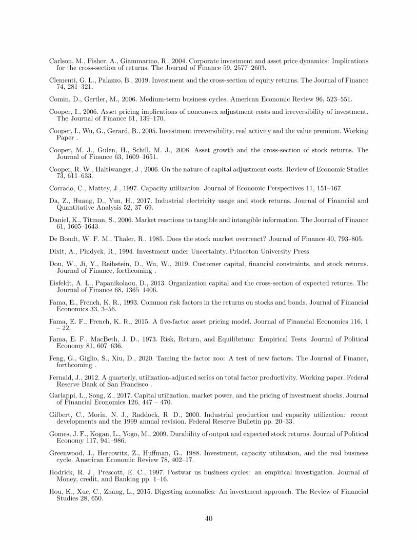
Carlson, M., Fisher, A., Giammarino, R., 2004. Corporate investment and asset price dynamics: Implicationsfor the cross-section of returns. The Journal of Finance 59, 2577–2603.

Clementi, G. L., Palazzo, B., 2019. Investment and the cross-section of equity returns. The Journal of Finance74, 281–321.

Comin, D., Gertler, M., 2006. Medium-term business cycles. American Economic Review 96, 523–551.

Cooper, I., 2006. Asset pricing implications of nonconvex adjustment costs and irreversibility of investment.The Journal of Finance 61, 139–170.

Cooper, I., Wu, G., Gerard, B., 2005. Investment irreversibility, real activity and the value premium. WorkingPaper .

Cooper, M. J., Gulen, H., Schill, M. J., 2008. Asset growth and the cross-section of stock returns. TheJournal of Finance 63, 1609–1651.

Cooper, R. W., Haltiwanger, J., 2006. On the nature of capital adjustment costs. Review of Economic Studies73, 611–633.

Corrado, C., Mattey, J., 1997. Capacity utilization. Journal of Economic Perspectives 11, 151–167.

Da, Z., Huang, D., Yun, H., 2017. Industrial electricity usage and stock returns. Journal of Financial andQuantitative Analysis 52, 37–69.

Daniel, K., Titman, S., 2006. Market reactions to tangible and intangible information. The Journal of Finance61, 1605–1643.

De Bondt, W. F. M., Thaler, R., 1985. Does the stock market overreact? Journal of Finance 40, 793–805.

Dixit, A., Pindyck, R., 1994. Investment under Uncertainty. Princeton University Press.

Dou, W., Ji, Y., Reibstein, D., Wu, W., 2019. Customer capital, financial constraints, and stock returns.Journal of Finance, forthcoming .

Eisfeldt, A. L., Papanikolaou, D., 2013. Organization capital and the cross-section of expected returns. TheJournal of Finance 68, 1365–1406.

Fama, E., French, K. R., 1993. Common risk factors in the returns on stocks and bonds. Journal of FinancialEconomics 33, 3–56.

Fama, E. F., French, K. R., 2015. A five-factor asset pricing model. Journal of Financial Economics 116, 1– 22.

Fama, E. F., MacBeth, J. D., 1973. Risk, Return, and Equilibrium: Empirical Tests. Journal of PoliticalEconomy 81, 607–636.

Feng, G., Giglio, S., Xiu, D., 2020. Taming the factor zoo: A test of new factors. The Journal of Finance,forthcoming .

Fernald, J., 2012. A quarterly, utilization-adjusted series on total factor productivity. Working paper. FederalReserve Bank of San Francisco .

Garlappi, L., Song, Z., 2017. Capital utilization, market power, and the pricing of investment shocks. Journalof Financial Economics 126, 447 – 470.

Gilbert, C., Morin, N. J., Raddock, R. D., 2000. Industrial production and capacity utilization: recentdevelopments and the 1999 annual revision. Federal Reserve Bulletin pp. 20–33.

Gomes, J. F., Kogan, L., Yogo, M., 2009. Durability of output and expected stock returns. Journal of PoliticalEconomy 117, 941–986.

Greenwood, J., Hercowitz, Z., Huffman, G., 1988. Investment, capacity utilization, and the real businesscycle. American Economic Review 78, 402–17.

Hodrick, R. J., Prescott, E. C., 1997. Postwar us business cycles: an empirical investigation. Journal ofMoney, credit, and Banking pp. 1–16.

Hou, K., Xue, C., Zhang, L., 2015. Digesting anomalies: An investment approach. The Review of FinancialStudies 28, 650.

40

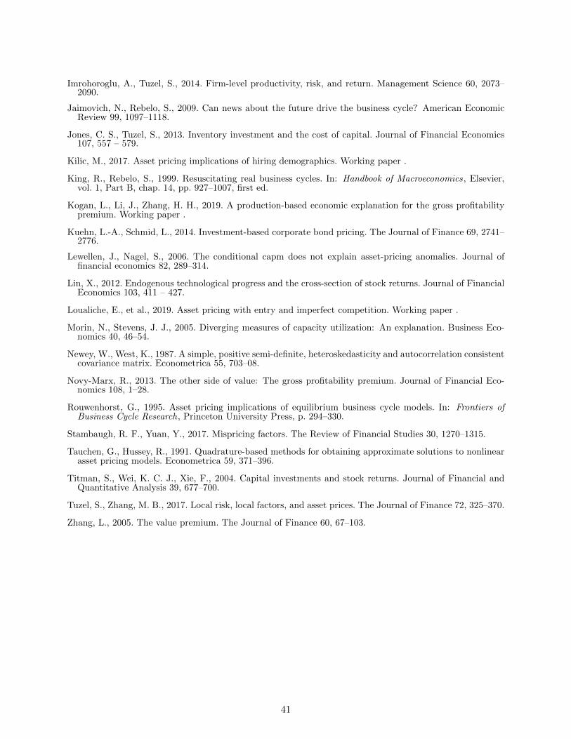
Imrohoroglu, A., Tuzel, S., 2014. Firm-level productivity, risk, and return. Management Science 60, 2073–2090.

Jaimovich, N., Rebelo, S., 2009. Can news about the future drive the business cycle? American EconomicReview 99, 1097–1118.

Jones, C. S., Tuzel, S., 2013. Inventory investment and the cost of capital. Journal of Financial Economics107, 557 – 579.

Kilic, M., 2017. Asset pricing implications of hiring demographics. Working paper .

King, R., Rebelo, S., 1999. Resuscitating real business cycles. In: Handbook of Macroeconomics, Elsevier,vol. 1, Part B, chap. 14, pp. 927–1007, first ed.

Kogan, L., Li, J., Zhang, H. H., 2019. A production-based economic explanation for the gross profitabilitypremium. Working paper .

Kuehn, L.-A., Schmid, L., 2014. Investment-based corporate bond pricing. The Journal of Finance 69, 2741–2776.

Lewellen, J., Nagel, S., 2006. The conditional capm does not explain asset-pricing anomalies. Journal offinancial economics 82, 289–314.

Lin, X., 2012. Endogenous technological progress and the cross-section of stock returns. Journal of FinancialEconomics 103, 411 – 427.

Loualiche, E., et al., 2019. Asset pricing with entry and imperfect competition. Working paper .

Morin, N., Stevens, J. J., 2005. Diverging measures of capacity utilization: An explanation. Business Eco-nomics 40, 46–54.

Newey, W., West, K., 1987. A simple, positive semi-definite, heteroskedasticity and autocorrelation consistentcovariance matrix. Econometrica 55, 703–08.

Novy-Marx, R., 2013. The other side of value: The gross profitability premium. Journal of Financial Eco-nomics 108, 1–28.

Rouwenhorst, G., 1995. Asset pricing implications of equilibrium business cycle models. In: Frontiers ofBusiness Cycle Research, Princeton University Press, p. 294–330.

Stambaugh, R. F., Yuan, Y., 2017. Mispricing factors. The Review of Financial Studies 30, 1270–1315.

Tauchen, G., Hussey, R., 1991. Quadrature-based methods for obtaining approximate solutions to nonlinearasset pricing models. Econometrica 59, 371–396.

Titman, S., Wei, K. C. J., Xie, F., 2004. Capital investments and stock returns. Journal of Financial andQuantitative Analysis 39, 677–700.

Tuzel, S., Zhang, M. B., 2017. Local risk, local factors, and asset prices. The Journal of Finance 72, 325–370.

Zhang, L., 2005. The value premium. The Journal of Finance 60, 67–103.

41

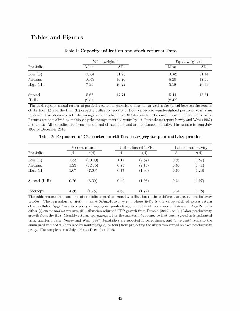
Tables and Figures

Table 1: Capacity utilization and stock returns: Data

Value-weighted Equal-weighted

Portfolio Mean SD Mean SD

Low (L) 13.64 21.23 10.62 21.14

Medium 10.49 16.70 8.20 17.63

High (H) 7.96 20.22 5.18 20.39

Spread 5.67 17.71 5.44 15.51

(L-H) (2.31) (2.47)

The table reports annual returns of portfolios sorted on capacity utilization, as well as the spread between the returns

of the Low (L) and the High (H) capacity utilization portfolio. Both value- and equal-weighted portfolio returns are

reported. The Mean refers to the average annual return, and SD denotes the standard deviation of annual returns.

Returns are annualized by multiplying the average monthly return by 12. Parentheses report Newey and West (1987)

t-statistics. All portfolios are formed at the end of each June and are rebalanced annually. The sample is from July

1967 to December 2015.

Table 2: Exposure of CU-sorted portfolios to aggregate productivity proxies

Market returns Util.-adjusted TFP Labor productivity

Portfolio β t(β) β t(β) β t(β)

Low (L) 1.33 (10.09) 1.17 (2.67) 0.95 (1.87)

Medium 1.23 (12.15) 0.75 (2.18) 0.60 (1.41)

High (H) 1.07 (7.68) 0.77 (1.93) 0.60 (1.28)

Spread (L-H) 0.26 (3.50) 0.40 (1.93) 0.34 (1.97)

Intercept 4.36 (1.78) 4.60 (1.72) 3.34 (1.18)

The table reports the exposures of portfolios sorted on capacity utilization to three different aggregate productivity

proxies. The regression is: Retei,t = β0 + β1Agg-Proxyt + εi,t, where Retei,t is the value-weighted excess return

of a portfolio, Agg-Proxy is a proxy of aggregate productivity, and β is the exposure of interest. Agg-Proxy is

either (i) excess market returns, (ii) utilization-adjusted TFP growth from Fernald (2012), or (iii) labor productivity

growth from the BLS. Monthly returns are aggregated to the quarterly frequency so that each regression is estimated

using quarterly data. Newey and West (1987) t-statistics are reported in parentheses, and “Intercept” refers to the

annualized value of β0 (obtained by multiplying β0 by four) from projecting the utilization spread on each productivity

proxy. The sample spans July 1967 to December 2015.

42

Table 3: Characteristics of capacity utilization sorted portfolios

Low (L) Medium High (H) Diff(L-H) t(Diff)

Panel A: Portfolio constituents

CU (%) 67 79 91

N (Stocks) 617 4423 348

N (Ind.) 5 35 4

Panel B: Portfolio characteristics

ME ($b) 1.02 0.81 1.08 -0.06 (-0.59)

BE / ME 1.34 1.19 1.13 0.21 (1.81)

ROA 0.02 0.01 0.01 0.00 (0.27)

GP / Assets 0.35 0.34 0.30 0.05 (1.27)

Asset Growth (%) 10.01 11.25 13.04 -3.03 (-1.08)

Inventory Growth (%) 10.29 10.59 12.62 -2.34 (-0.37)

I / K 0.06 0.06 0.09 -0.03 (-2.03)

IVOL (%) 3.18 2.89 2.86 0.32 (1.96)

TFP 0.76 0.73 0.78 -0.02 (-0.51)

Hire Rate (%) 3.95 3.48 5.80 -1.85 (-0.68)

R&D / ME 0.06 0.05 0.05 0.01 (0.97)

OC / AT 1.31 1.21 0.73 0.57 (1.12)

Leverage 0.26 0.24 0.26 -0.01 (-0.76)

Debt growth (%) 3.64 2.80 5.32 -1.68 (-1.38)

Equity issue. (%) 4.78 5.19 5.38 -0.60 (-1.46)

The table shows both the composition and characteristics of capacity utilization sorted portfolios. Panel A reports the

composition of each portfolio, while Panel B reports industry-level characteristics, averaged across all industries that

are assigned to a particular portfolio. All data is annual and is recorded at the end of each June from 1967 to 2015. In

Panel A, CU denotes the capacity utilization rate, while N (Stocks) and N (Industries) refer to the average number of

individual firms and industries comprising each portfolio, respectively. In Panel B, all statistics are computed as the

time-series average of each portfolio’s simple firm-level average of a certain characteristic. Details on the construction

of each variable are provided in Section OA.1 of the Online Appendix. The column Diff(L-H) refers to the difference

between the average characteristics of the low and high capacity utilization portfolios, and t(Diff) is the Newey and

West (1987) t-statistic associated with this difference.

43

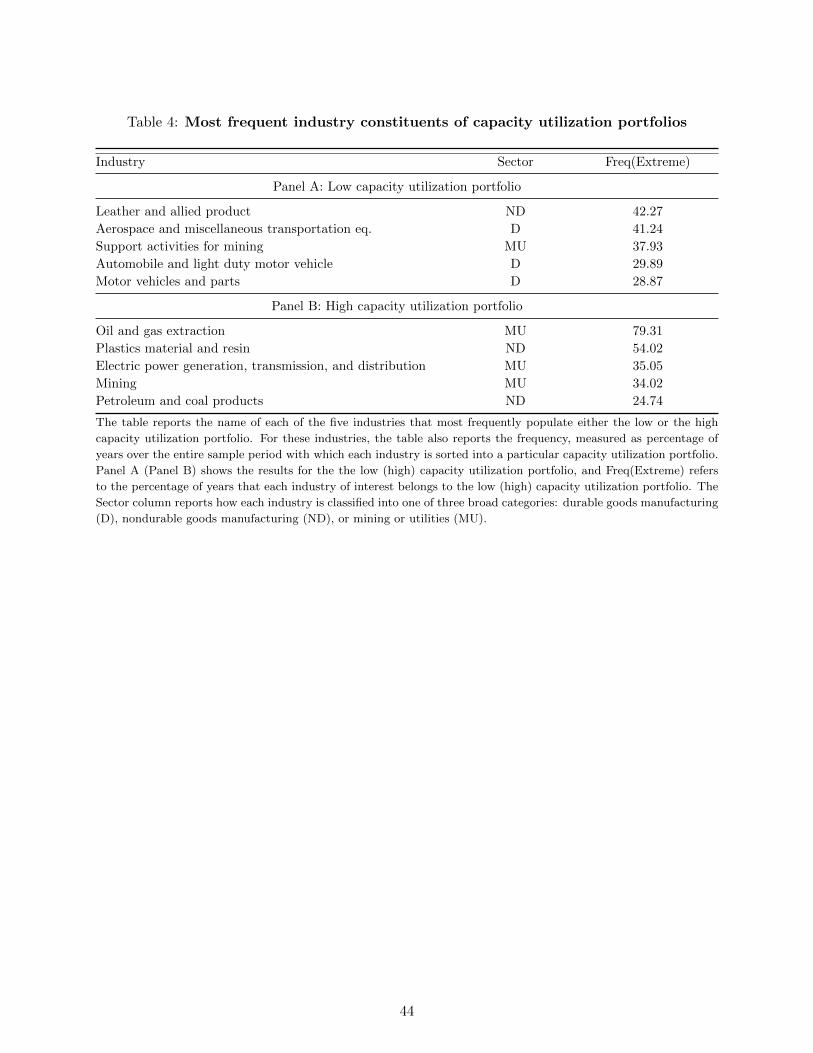
Table 4: Most frequent industry constituents of capacity utilization portfolios

Industry Sector Freq(Extreme)

Panel A: Low capacity utilization portfolio

Leather and allied product ND 42.27

Aerospace and miscellaneous transportation eq. D 41.24

Support activities for mining MU 37.93

Automobile and light duty motor vehicle D 29.89

Motor vehicles and parts D 28.87

Panel B: High capacity utilization portfolio

Oil and gas extraction MU 79.31

Plastics material and resin ND 54.02

Electric power generation, transmission, and distribution MU 35.05

Mining MU 34.02

Petroleum and coal products ND 24.74

The table reports the name of each of the five industries that most frequently populate either the low or the high

capacity utilization portfolio. For these industries, the table also reports the frequency, measured as percentage of

years over the entire sample period with which each industry is sorted into a particular capacity utilization portfolio.

Panel A (Panel B) shows the results for the the low (high) capacity utilization portfolio, and Freq(Extreme) refers

to the percentage of years that each industry of interest belongs to the low (high) capacity utilization portfolio. The

Sector column reports how each industry is classified into one of three broad categories: durable goods manufacturing

(D), nondurable goods manufacturing (ND), or mining or utilities (MU).

44

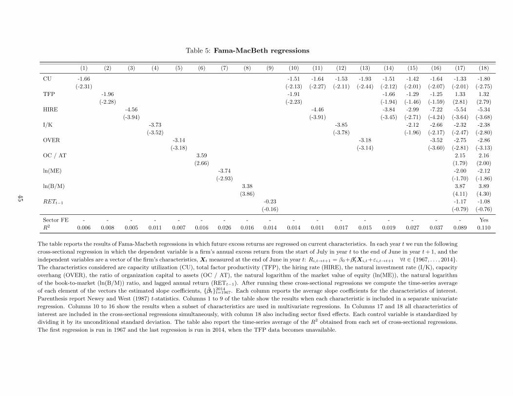
Table 5: Fama-MacBeth regressions

(1) (2) (3) (4) (5) (6) (7) (8) (9) (10) (11) (12) (13) (14) (15) (16) (17) (18)

CU -1.66 -1.51 -1.64 -1.53 -1.93 -1.51 -1.42 -1.64 -1.33 -1.80

(-2.31) (-2.13) (-2.27) (-2.11) (-2.44) (-2.12) (-2.01) (-2.07) (-2.01) (-2.75)

TFP -1.96 -1.91 -1.66 -1.29 -1.25 1.33 1.32

(-2.28) (-2.23) (-1.94) (-1.46) (-1.59) (2.81) (2.79)

HIRE -4.56 -4.46 -3.84 -2.99 -7.22 -5.54 -5.34

(-3.94) (-3.91) (-3.45) (-2.71) (-4.24) (-3.64) (-3.68)

I/K -3.73 -3.85 -2.12 -2.66 -2.32 -2.38

(-3.52) (-3.78) (-1.96) (-2.17) (-2.47) (-2.80)

OVER -3.14 -3.18 -3.52 -2.75 -2.86

(-3.18) (-3.14) (-3.60) (-2.81) (-3.13)

OC / AT 3.59 2.15 2.16

(2.66) (1.79) (2.00)

ln(ME) -3.74 -2.00 -2.12

(-2.93) (-1.70) (-1.86)

ln(B/M) 3.38 3.87 3.89

(3.86) (4.11) (4.30)

RETt−1 -0.23 -1.17 -1.08

(-0.16) (-0.79) (-0.76)

Sector FE - - - - - - - - - - - - - - - - - Yes

R2 0.006 0.008 0.005 0.011 0.007 0.016 0.026 0.016 0.014 0.014 0.011 0.017 0.015 0.019 0.027 0.037 0.089 0.110

The table reports the results of Fama-Macbeth regressions in which future excess returns are regressed on current characteristics. In each year t we run the following

cross-sectional regression in which the dependent variable is a firm’s annual excess return from the start of July in year t to the end of June in year t+ 1, and the

independent variables are a vector of the firm’s characteristics, Xt measured at the end of June in year t: Ri,t→t+1 = β0+β′tXi,t+εi,t→t+1 ∀t ∈ {1967, . . . , 2014}.The characteristics considered are capacity utilization (CU), total factor productivity (TFP), the hiring rate (HIRE), the natural investment rate (I/K), capacity

overhang (OVER), the ratio of organization capital to assets (OC / AT), the natural logarithm of the market value of equity (ln(ME)), the natural logarithm

of the book-to-market (ln(B/M)) ratio, and lagged annual return (RETt−1). After running these cross-sectional regressions we compute the time-series average

of each element of the vectors the estimated slope coefficients, {βt}2014t=1967. Each column reports the average slope coefficients for the characteristics of interest.

Parenthesis report Newey and West (1987) t-statistics. Columns 1 to 9 of the table show the results when each characteristic is included in a separate univariate

regression. Columns 10 to 16 show the results when a subset of characteristics are used in multivariate regressions. In Columns 17 and 18 all characteristics of

interest are included in the cross-sectional regressions simultaneously, with column 18 also including sector fixed effects. Each control variable is standardized by

dividing it by its unconditional standard deviation. The table also report the time-series average of the R2 obtained from each set of cross-sectional regressions.

The first regression is run in 1967 and the last regression is run in 2014, when the TFP data becomes unavailable.

45

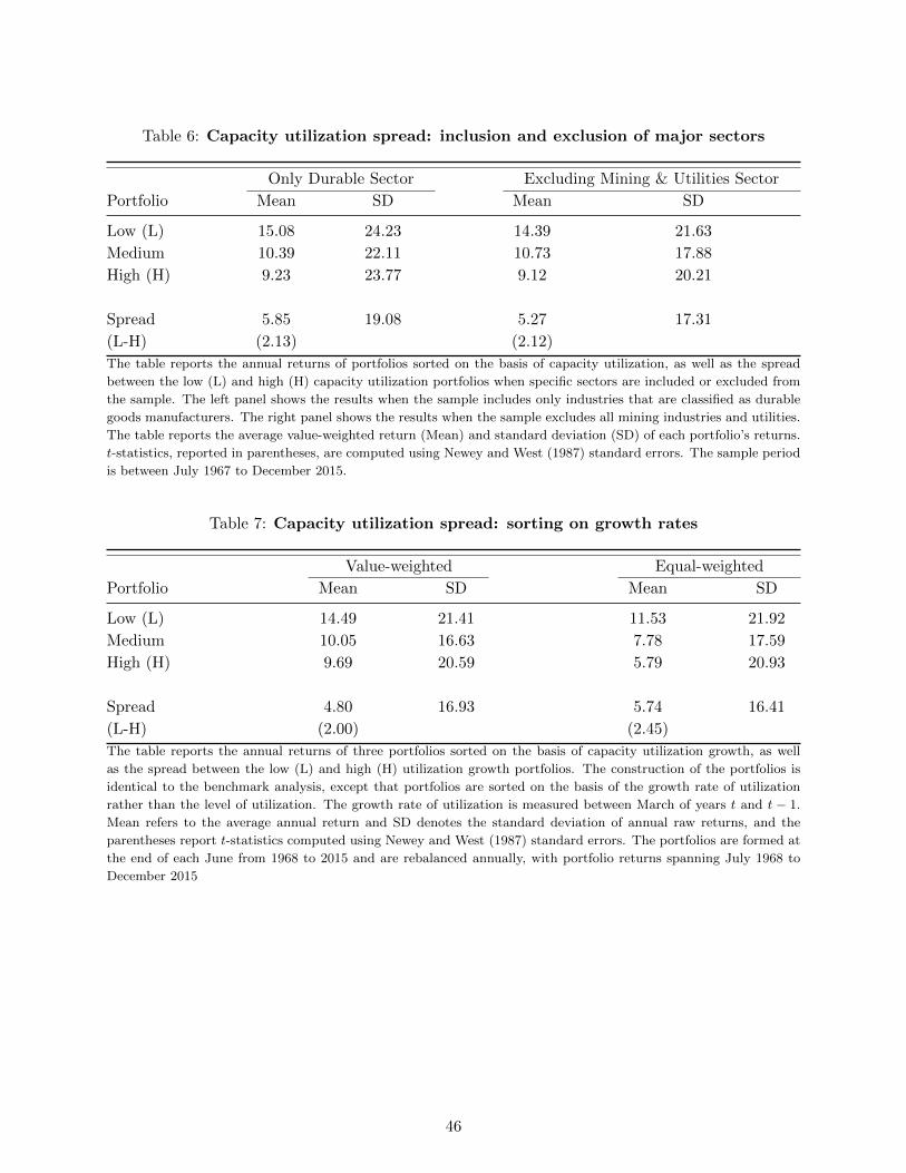
Table 6: Capacity utilization spread: inclusion and exclusion of major sectors

Only Durable Sector Excluding Mining & Utilities Sector

Portfolio Mean SD Mean SD

Low (L) 15.08 24.23 14.39 21.63

Medium 10.39 22.11 10.73 17.88

High (H) 9.23 23.77 9.12 20.21

Spread 5.85 19.08 5.27 17.31

(L-H) (2.13) (2.12)

The table reports the annual returns of portfolios sorted on the basis of capacity utilization, as well as the spread

between the low (L) and high (H) capacity utilization portfolios when specific sectors are included or excluded from

the sample. The left panel shows the results when the sample includes only industries that are classified as durable

goods manufacturers. The right panel shows the results when the sample excludes all mining industries and utilities.

The table reports the average value-weighted return (Mean) and standard deviation (SD) of each portfolio’s returns.

t-statistics, reported in parentheses, are computed using Newey and West (1987) standard errors. The sample period

is between July 1967 to December 2015.

Table 7: Capacity utilization spread: sorting on growth rates

Value-weighted Equal-weighted

Portfolio Mean SD Mean SD

Low (L) 14.49 21.41 11.53 21.92

Medium 10.05 16.63 7.78 17.59

High (H) 9.69 20.59 5.79 20.93

Spread 4.80 16.93 5.74 16.41

(L-H) (2.00) (2.45)

The table reports the annual returns of three portfolios sorted on the basis of capacity utilization growth, as well

as the spread between the low (L) and high (H) utilization growth portfolios. The construction of the portfolios is

identical to the benchmark analysis, except that portfolios are sorted on the basis of the growth rate of utilization

rather than the level of utilization. The growth rate of utilization is measured between March of years t and t − 1.

Mean refers to the average annual return and SD denotes the standard deviation of annual raw returns, and the

parentheses report t-statistics computed using Newey and West (1987) standard errors. The portfolios are formed at

the end of each June from 1968 to 2015 and are rebalanced annually, with portfolio returns spanning July 1968 to

December 2015

46

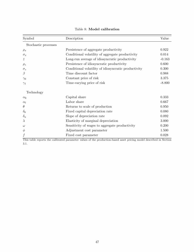
Table 8: Model calibration

Symbol Description Value

Stochastic processes

ρx Persistence of aggregate productivity 0.922

σx Conditional volatility of aggregate productivity 0.014

z Long-run average of idiosyncratic productivity -0.163

ρz Persistence of idiosyncratic productivity 0.600

σz Conditional volatility of idiosyncratic productivity 0.300

β Time discount factor 0.988

γ0 Constant price of risk 3.375

γ1 Time-varying price of risk -8.800

Technology

αk Capital share 0.333

αl Labor share 0.667

θ Returns to scale of production 0.950

δk Fixed capital depreciation rate 0.080

δu Slope of depreciation rate 0.092

λ Elasticity of marginal depreciation 3.000

ω Sensitivity of wages to aggregate productivity 0.200

φ Adjustment cost parameter 1.500

f Fixed cost parameter 0.028

This table reports the calibrated parameter values of the production-based asset pricing model described in Section

3.1.

47

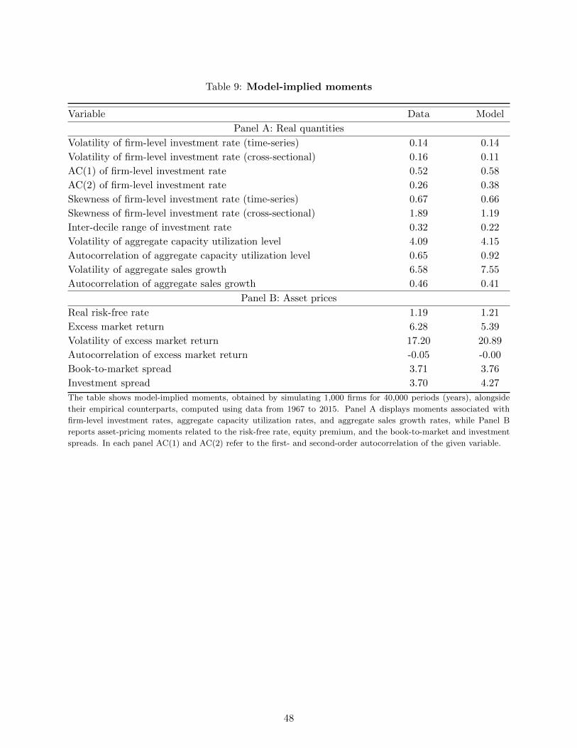
Table 9: Model-implied moments

Variable Data Model

Panel A: Real quantities

Volatility of firm-level investment rate (time-series) 0.14 0.14

Volatility of firm-level investment rate (cross-sectional) 0.16 0.11

AC(1) of firm-level investment rate 0.52 0.58

AC(2) of firm-level investment rate 0.26 0.38

Skewness of firm-level investment rate (time-series) 0.67 0.66

Skewness of firm-level investment rate (cross-sectional) 1.89 1.19

Inter-decile range of investment rate 0.32 0.22

Volatility of aggregate capacity utilization level 4.09 4.15

Autocorrelation of aggregate capacity utilization level 0.65 0.92

Volatility of aggregate sales growth 6.58 7.55

Autocorrelation of aggregate sales growth 0.46 0.41

Panel B: Asset prices

Real risk-free rate 1.19 1.21

Excess market return 6.28 5.39

Volatility of excess market return 17.20 20.89

Autocorrelation of excess market return -0.05 -0.00

Book-to-market spread 3.71 3.76

Investment spread 3.70 4.27

The table shows model-implied moments, obtained by simulating 1,000 firms for 40,000 periods (years), alongside

their empirical counterparts, computed using data from 1967 to 2015. Panel A displays moments associated with

firm-level investment rates, aggregate capacity utilization rates, and aggregate sales growth rates, while Panel B

reports asset-pricing moments related to the risk-free rate, equity premium, and the book-to-market and investment

spreads. In each panel AC(1) and AC(2) refer to the first- and second-order autocorrelation of the given variable.

48

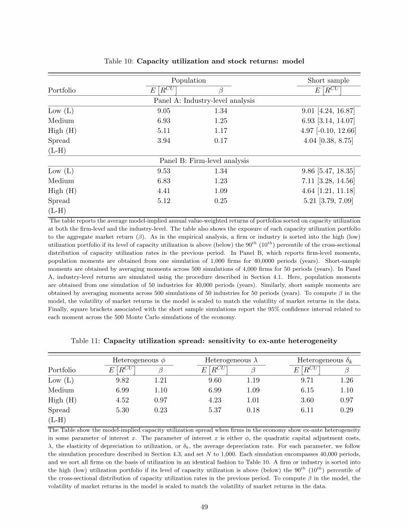
Table 10: Capacity utilization and stock returns: model

Population Short sample

Portfolio E[RCU

]β E

[RCU

]Panel A: Industry-level analysis

Low (L) 9.05 1.34 9.01 [4.24, 16.87]

Medium 6.93 1.25 6.93 [3.14, 14.07]

High (H) 5.11 1.17 4.97 [-0.10, 12.66]

Spread 3.94 0.17 4.04 [0.38, 8.75]

(L-H)

Panel B: Firm-level analysis

Low (L) 9.53 1.34 9.86 [5.47, 18.35]

Medium 6.83 1.23 7.11 [3.28, 14.56]

High (H) 4.41 1.09 4.64 [1.21, 11.18]

Spread 5.12 0.25 5.21 [3.79, 7.09]

(L-H)

The table reports the average model-implied annual value-weighted returns of portfolios sorted on capacity utilization

at both the firm-level and the industry-level. The table also shows the exposure of each capacity utilization portfolio

to the aggregate market return (β). As in the empirical analysis, a firm or industry is sorted into the high (low)

utilization portfolio if its level of capacity utilization is above (below) the 90th (10th) percentile of the cross-sectional

distribution of capacity utilization rates in the previous period. In Panel B, which reports firm-level moments,

population moments are obtained from one simulation of 1,000 firms for 40,0000 periods (years). Short-sample

moments are obtained by averaging moments across 500 simulations of 4,000 firms for 50 periods (years). In Panel

A, industry-level returns are simulated using the procedure described in Section 4.1. Here, population moments

are obtained from one simulation of 50 industries for 40,000 periods (years). Similarly, short sample moments are

obtained by averaging moments across 500 simulations of 50 industries for 50 periods (years). To compute β in the

model, the volatility of market returns in the model is scaled to match the volatility of market returns in the data.

Finally, square brackets associated with the short sample simulations report the 95% confidence interval related to

each moment across the 500 Monte Carlo simulations of the economy.

Table 11: Capacity utilization spread: sensitivity to ex-ante heterogeneity

Heterogeneous φ Heterogeneous λ Heterogeneous δkPortfolio E

[RCU

]β E

[RCU

]β E

[RCU

]β

Low (L) 9.82 1.21 9.60 1.19 9.71 1.26

Medium 6.99 1.10 6.99 1.09 6.15 1.10

High (H) 4.52 0.97 4.23 1.01 3.60 0.97

Spread 5.30 0.23 5.37 0.18 6.11 0.29

(L-H)

The Table show the model-implied capacity utilization spread when firms in the economy show ex-ante heterogeneity

in some parameter of interest x. The parameter of interest x is either φ, the quadratic capital adjustment costs,

λ, the elasticity of depreciation to utilization, or δk, the average depreciation rate. For each parameter, we follow

the simulation procedure described in Section 4.3, and set N to 1,000. Each simulation encompasses 40,000 periods,

and we sort all firms on the basis of utilization in an identical fashion to Table 10. A firm or industry is sorted into

the high (low) utilization portfolio if its level of capacity utilization is above (below) the 90th (10th) percentile of

the cross-sectional distribution of capacity utilization rates in the previous period. To compute β in the model, the

volatility of market returns in the model is scaled to match the volatility of market returns in the data.

49

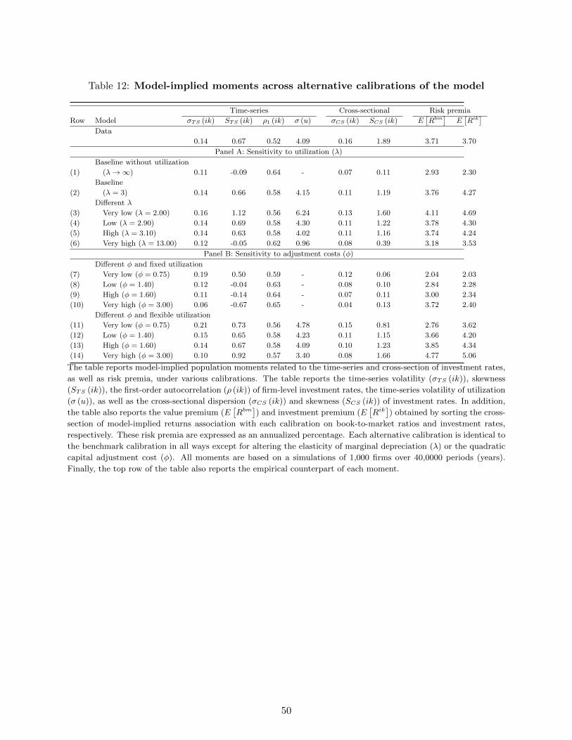
Table 12: Model-implied moments across alternative calibrations of the model

Time-series Cross-sectional Risk premia

Row Model σTS (ik) STS (ik) ρ1 (ik) σ (u) σCS (ik) SCS (ik) E[Rbm

]E[Rik

]Data

0.14 0.67 0.52 4.09 0.16 1.89 3.71 3.70

Panel A: Sensitivity to utilization (λ)

Baseline without utilization

(1) (λ→∞) 0.11 -0.09 0.64 - 0.07 0.11 2.93 2.30

Baseline

(2) (λ = 3) 0.14 0.66 0.58 4.15 0.11 1.19 3.76 4.27

Different λ

(3) Very low (λ = 2.00) 0.16 1.12 0.56 6.24 0.13 1.60 4.11 4.69

(4) Low (λ = 2.90) 0.14 0.69 0.58 4.30 0.11 1.22 3.78 4.30

(5) High (λ = 3.10) 0.14 0.63 0.58 4.02 0.11 1.16 3.74 4.24

(6) Very high (λ = 13.00) 0.12 -0.05 0.62 0.96 0.08 0.39 3.18 3.53

Panel B: Sensitivity to adjustment costs (φ)

Different φ and fixed utilization

(7) Very low (φ = 0.75) 0.19 0.50 0.59 - 0.12 0.06 2.04 2.03

(8) Low (φ = 1.40) 0.12 -0.04 0.63 - 0.08 0.10 2.84 2.28

(9) High (φ = 1.60) 0.11 -0.14 0.64 - 0.07 0.11 3.00 2.34

(10) Very high (φ = 3.00) 0.06 -0.67 0.65 - 0.04 0.13 3.72 2.40

Different φ and flexible utilization

(11) Very low (φ = 0.75) 0.21 0.73 0.56 4.78 0.15 0.81 2.76 3.62

(12) Low (φ = 1.40) 0.15 0.65 0.58 4.23 0.11 1.15 3.66 4.20

(13) High (φ = 1.60) 0.14 0.67 0.58 4.09 0.10 1.23 3.85 4.34

(14) Very high (φ = 3.00) 0.10 0.92 0.57 3.40 0.08 1.66 4.77 5.06

The table reports model-implied population moments related to the time-series and cross-section of investment rates,

as well as risk premia, under various calibrations. The table reports the time-series volatility (σTS (ik)), skewness

(STS (ik)), the first-order autocorrelation (ρ (ik)) of firm-level investment rates, the time-series volatility of utilization

(σ (u)), as well as the cross-sectional dispersion (σCS (ik)) and skewness (SCS (ik)) of investment rates. In addition,

the table also reports the value premium (E[Rbm

]) and investment premium (E

[Rik

]) obtained by sorting the cross-

section of model-implied returns association with each calibration on book-to-market ratios and investment rates,

respectively. These risk premia are expressed as an annualized percentage. Each alternative calibration is identical to

the benchmark calibration in all ways except for altering the elasticity of marginal depreciation (λ) or the quadratic

capital adjustment cost (φ). All moments are based on a simulations of 1,000 firms over 40,0000 periods (years).

Finally, the top row of the table also reports the empirical counterpart of each moment.

50

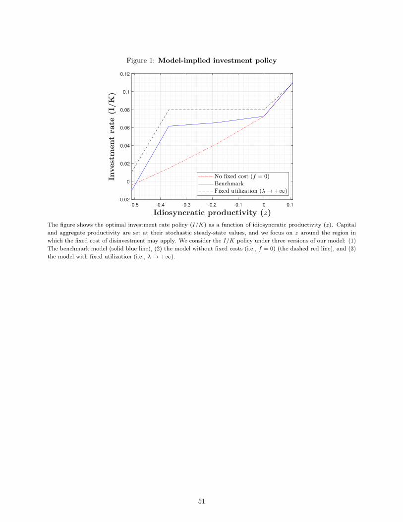
Figure 1: Model-implied investment policy

-0.5 -0.4 -0.3 -0.2 -0.1 0 0.1

-0.02

0

0.02

0.04

0.06

0.08

0.1

0.12

The figure shows the optimal investment rate policy (I/K) as a function of idiosyncratic productivity (z). Capital

and aggregate productivity are set at their stochastic steady-state values, and we focus on z around the region in

which the fixed cost of disinvestment may apply. We consider the I/K policy under three versions of our model: (1)

The benchmark model (solid blue line), (2) the model without fixed costs (i.e., f = 0) (the dashed red line), and (3)

the model with fixed utilization (i.e., λ→ +∞).

51

A Internet appendix

OA.1 Variable description and construction

Asset growth. Asset growth is calculated as the year-on-year annual growth rate of total

assets (Compustat Annual item AT) betweens years t− 1 and t. This definition of asset growth is

drawn from Cooper, Gulen, and Schill (2008).

Book-to-market (BE/ME). A firm’s book-to-market ratio is constructed by following Daniel

and Titman (2006). Book equity is defined as shareholders’ equity minus the value of preferred

stock. If available, shareholders’ equity is set equal to stockholders’ equity (Compustat Annual

item SEQ). If stockholders’ equity is missing, then common equity (Compustat Annual item CEQ)

plus the par value of preferred stock (Compustat Annual item PSTK) is used instead. If neither of

the two previous definitions of stockholders’ equity can be constructed, then shareholders’ equity is

the difference between total assets (Compustat Annual item AT) and total liabilities (Compustat

Annual item LT). For the value of preferred stock we use the redemption value (Compustat Annual

item PSTKRV), the liquidating value (Compustat Annual item PSTKL), or the carrying value

(Compustat Annual item PSTK), in that order of preference. We also add the value of deferred

taxes and investment tax credits (Compustat Annual item TXDITC) to, and subtract the value of

post retirement benefits (Compustat Annual item PRBA) from, the value of book equity if either

variable is available. Finally, the book value of equity in the fiscal year ending in calendar year

t− 1 is divided by the market value of common equity from December of year t− 1.

Capacity. The capacity estimate measures the maximum amount of output that an indus-

try can produce, assuming the sufficient availability of inputs to production and a realistic work

schedule. The FRB relies on a variety of sources to determine the capacity of each industry. The

primary source of capacity data for manufacturing industries, which make up the bulk of our sam-

ple, is currently the Quarterly Survey of Plant Capacity Utilization (QPC). For approximately 20%

industries, including a subset of manufacturers, capacity is reported in physical units obtained from

government or trade sources, such as the United States Geological Survey. Finally, for a small pro-

portion of industries for which neither of the aforementioned data sources are available, the FRB

estimates capacity based on trends through peaks in production. Gilbert, Morin, and Raddock

(2000) and Board of Govenors of the Federal Reserve System (2017) provide overviews of how the

FRB measures capacity.

Capacity overhang (OVER). We construct a monthly measure of capacity overhang by

following the procedure described by Aretz and Pope (2018). In particular we recursively estimate

equation (1) of Aretz and Pope (2018) using total assets (Compustat Annual item AT) as our

measure of installed capacity.

Debt growth. We measure the growth rate of a firm’s debt by calculating the annual per-

centage change in outstanding total debt, expressed in real terms. We define total real debt as the

sum of long-term debt (Compustat Annual item DLTT) and debt in current liabilities (Compustat

Annual item DLC), scaled by the value of the consumer price index. When computing this quantity

we require firms to have at least $10m of debt outstanding in year t− 1.

Depreciation rate (BEA implied). To compute the BEA-implied depreciation rate we take

Internet appendix - p.1

the GDP-weighted average of the industry-level depreciation rates associated with equipment and

structures.

Depreciation rate (Compustat implied). We compute Compustat-implied industry-level

depreciation rates by first constructing firm-level depreciation rates. A firm’s depreciation rate is

defined as the firm’s depreciation expense (Compustat annual item DP) minus the firm’s amor-

tization (Compustat annual item AM) scaled by net property, plant, and equipment (Compustat

annual item PPENT). We then aggregate these firm-level depreciation rates to the industry-level

by computing the value-weighted depreciation rate across all firms assigned to a particular industry.

Equity issuance. Gross equity issuance is defined as the sale of common and preferred stock

(Compustat Annual item SSTK) divided by the lagged value of book equity, as per Belo et al.

(2018).

Gross profitability (GP). Consistent with Novy-Marx (2013), gross profitability is calculated

as total revenue (Compustat Annual item REVT) minus the cost of goods sold (Compustat Annual

item COGS), divided by total assets (Compustat Annual item AT).

Hiring rate. The hiring rate is computed following Belo et al. (2014a). Specifically, the hiring

rate in year t is the change in the number of employees (Compustat Annual item EMP) from year

t− 1 to year t, divided by the mean employees over years t− 1 and t.

Idiosyncratic volatility (IVOL). Idiosyncratic volatility is computed in accordance with

Ang et al. (2006). At the end of month t, a firm’s idiosyncratic volatility over the past month is

obtained by regressing its daily excess returns on the Fama and French (1993) factors, provided

there are at least 15 valid daily returns in the month. Idiosyncratic volatility is then defined as the

standard deviation of the residuals from the aforementioned regression.

Intangible investment rate (R&D / ME). We follow Lin (2012) and define a firm’s

intangible investment rate as the firm’s R&D expense (Compustat Annual item XRD) divided by

the firm’s market capitalization.

Inventory growth. The inventory growth rate is defined following Belo and Lin (2012). That

is, we compute the annual percentage change in each firm’s inventory holdings (Compustat Annual

item INVT) after converting the value of inventories to real terms.

Investment rate. We follow Stambaugh and Yuan (2017) and compute the investment rate

as the change in gross property, plant, and equipment (Compustat Annual item PPEGT) plus the

change in inventory (Compustat Annual item INVT) between years t − 1 and t, divided by the

value of total assets (Compustat Annual item AT) in year t− 1.

Leverage. We define a firm’s leverage ratio as long-term debt (Compustat Annual item DLTT)

plus debt in current liabilities (Compustat Annual item DLC) divided by total assets (Compustat

Annual item AT).

Market capitalization. A firm’s end of month t market capitalization is computed as the

firm’s end of month t stock price (CRSP Monthly item PRC) multiplied by the firm’s number of

shares outstanding (CRSP Monthly item SHROUT).

Natural investment rate. Following Belo et al. (2014a) the natural rate of investment is

computed as capital expenditure (Compustat Annual item CAPX) minus the sales of property,

planet, and equipment (Compustat Annual item SPPE) scaled by the average net property, planet,

and equipment in years t and t− 1 (Compustat Annual item PPENT). Missing values of SPPE are

set to zero.

Internet appendix - p.2

Organizational capital (OC). We construct the stock of a firm’s organizational capital by

following the perpetual inventory inventory method described by Eisfeldt and Papanikolaou (2013).

That is, we recursively accumulate a firm’s real selling, general and administrative expenses (Com-

pustat Annual item XSGA) over time, and scale the stock of organizational capital by the firm’s

total assets (Compustat Annual item AT).

Return-on-assets (ROA). Following Imrohoroglu and Tuzel (2014) return on assets (ROA)

is computed as net income before extraordinary items (Computat Annual item IB) minus preferred

dividends (Compustat Annual item DVP), if available, plus deferred income taxes (Compustat

Annual item TXDI), if available, scaled by total assets (Compustat Annual item AT).

TechMark. Recalling equation (27), total factor productivity (TFP) is comprised of three dis-

tinct components: technology, time-varying markups, and time-varying capacity utilization rates.

We isolate the components of TFP related to technology and markups, referred to as “TechMark,”

as follows. First, we obtain firm-level estimates of the natural logarithm of TFP from Imrohoroglu

and Tuzel (2014). We refer to this variable as ln (TFPi,t). Next, we assign industry-level capac-

ity utilization rates to individual firms by following the matching algorithm described in Section

OA.3.3. We take the natural logarithm of these firm firm-level capacity utilization rates, and

denote this quantity ln (CUi,t). Finally, we define the TechMark variable for firm i at time t as

TechMarki,t = ln (TFPi,t)− ln (CUi,t).

Total factor productivity (TFP). The firm-level estimates of TFP are drawn from Imro-

horoglu and Tuzel (2014).

OA.2 Capacity utilization data and summary statistics

The public report on industrial capacity utilization covers 57 industries. These industries are

defined at different levels of aggregation ranging from two- to six-digit North American Industry

Classification System (NAICS) codes. Specifically, 12 of the industries are crude aggregates that

span multiple two-digit NAICS codes. For example, one of these 12 aggregates includes the average

capacity utilization rate of all manufacturers in the U.S. We remove these 12 crude aggregates from

our benchmark sample for two reasons. First, these aggregates do not provide new information as

they are spanned by more granularly defined sub-industries that are also included in the sample.

Second, these aggregates represents a considerable proportion of total market value and would

consequently dominate the returns of the value-weighted portfolios we form in Section 2. Removing

these 12 crude aggregates leaves us with a benchmark cross-section of 45 industries that features a

mix of durable manufacturers, nondurable manufacturers, and miners and utilities.42

As the 45 industries included in the benchmark sample are defined from the relatively coarse

two-digit NAICS code level to the most granular six-digit NAICS code level, the benchmark cross-

section includes a number of overlapping industries.43 For instance, the capacity utilization rate

of food manufacturers is included in the utilization rate of two industries reported by the FRB:

“Food,” as well as “Food, beverage, and tobacco.” Since removing overlapping industries from our

42A list of these 45 industries, along with each industry’s sectoral affiliation, is provided in Table OA.2.1 of theOnline Appendix.

43In particular, our final sample consists of one sector defined at the two-digit NAICS level, 27 subsectors definedat the three-digit NAICS level, 13 industry groups defined at the four-digit NAICS level, two industries defined atthe five-digit NAICS level, and two U.S. industries defined at the six-digit NAICS level. In Section OA.3 we ensurethat our results are robust to this heterogeneity in classification levels.

Internet appendix - p.3

benchmark sample would significantly reduce the number of cross-sectional assets, and thus, make

certain asset pricing tests, such as portfolio double sorts, infeasible, we deal with this overlap in

two ways. First, in robustness section OA.3.1 we remove the industries that overlap with others

and conduct our baseline empirical tests in a sub-sample of 24 distinct non-overlapping industries,

each of which corresponds to a unique three-digit NAICS code. Following the example above, this

set of distinct industries includes both “Food”’ and “Beverage and Tobacco” manufacturers, but

excludes the composite index that covers both groups of manufacturers. Table OA.3.6 shows that

the utilization premium is significant even within this narrower sample. Second, we verify that our

results are not driven by any particular industry that dominates the sample (see Tables 4 and 6).

Monthly capacity utilization data for 32 industries is available beginning in January 1967, and

data for an additional 25 industries becomes available in January 1972.44 The capacity utilization

data we collect ends in December 2015, when we commenced the empirical analysis of the paper.

We verify in Section OA.3.1 that our results hold when we only consider the most recent half of

the sample period.

OA.2.1 Summary statistics

Below, we describe the properties of the aggregate capacity utilization rate and report summary

statistics related to the cross-section of industry-level utilization rates.

Figure OA.2.1 shows the annual growth rate of aggregate capacity utilization over the sample

period. The figure shows that capacity utilization fluctuates significantly over time and that the

growth rate of aggregate utilization is procylical. The aggregate utilization rate drops during reces-

sions, particularly during the Great Recession. The growth rate of aggregate capacity utilization

tends to slightly lead the business cycle, and has often served as an early warning for recessions.

In five out of the seven recessions during our sample period the growth rate of utilization begins to

drop prior to the start of the NBER defined recession. The growth rate of capacity utilization in-

creases during the technological revolution of the late 1990’s, the housing bubble, and the recovery

from the Great Recession.

As illustrated by equation (1), the capacity utilization rate is a combination of both industrial

production and capacity. The former variable is studied extensively in the macroeconomic and

finance literature, and features prominently in the context of asset pricing. For instance, Cooper

et al. (2008) document a premium for firms with lower total asset growth. The growth rate of assets

is directly linked to firms’ output, and is consequently captured by the FRB’s measure of industrial

production. To establish the empirical novelty in examining capacity utilization, we examine the

extent to which utilization fluctuates independently of industrial production using the following

projection:

∆CUt = β0 + β1∆IPt + εt. (22)

Here, ∆CUt (∆IPt) is annual growth rate of aggregate capacity utilization (industrial production),

and the residual εt captures the component of capacity utilization that is orthogonal to industrial

production. Figure OA.2.1 also displays this orthogonal component over the sample period. The

dynamics of this orthogonal component do not appear to reflect the dynamics of a white noise

process. εt is smoother than utilization growth, and changes in εt are largely procylical. Similar

44There are only 11 monthly time-series reported between January 1948 to December 1966. As eleven industries isa very small cross-section, we do not consider the pre-1967 period in our benchmark sample.

Internet appendix - p.4

to utilization growth, εt tends to drop during NBER recessions. In some instances the orthogonal

component also deviates significantly from capacity utilization growth. For example, during the

technology boom of mid-1990’s, the orthogonal component declines whereas capacity utilization

increases. The orthogonal component drops due to an acceleration in the growth of capacity that

was likely facilitated by the technological advancements of the era (Bansak, Morin, and Starr,

2007).

Table OA.2.2 reports summary statistics for the capacity utilization rates of each sector in our

benchmark sample. The average rate of aggregate capacity utilization rate is 79.91%. This figure

for the U.S. is close to the average capacity utilization rates of 81.17%, 84.69%, and 82.49% for the

Euro Zone, China, and Israel, respectively.45

The majority of the capacity utilization data in the sample pertains to the manufacturing sector,

with an almost even split between the number of durable and nondurable manufacturing industries.

The mean annual utilization rate is 77.39% (80.09%) for durable (nondurable) manufacturers. Each

of these rates is statistically indistinguishable from the average rate of capacity utilization across all

industries in the sample. The fact that the average capacity utilization rate of the manufacturing

sector, and of the durable and nondurable manufacturing subsectors, is not statistically different

from the U.S. average alleviates the concern that our results are driven by ex-ante heterogeneity

between sectors.

Among mining industries and utilities the average capacity utilization rate is 84.13%. This

average rate is slightly higher than, and statistically different from, the average rate across all

industries. Due to this difference in average capacity utilization rates we verify that our empirical

results are robust to excluding mining industries and utilities from our sample. We also verify

that our results still hold when we conduct tests using the growth rate of capacity utilization that

eliminates differences in levels by construction. The results of both of these tests are reported in

Section OA.3.

Table OA.2.2 also reports the volatility and autocorrelation of utilization for the different sectors

in our sample. The volatility of the capacity utilization rate is comparable across sectors and ranges

from 6.67% per annum for mining to 8.29% per annum for durables. The autocorrelation ranges

from 0.52 to 0.61, with an all-industry mean of 0.58. These statistics affirm the notion that the

level of utilization follows similar dynamics regardless of sector.

Overall, Table OA.2.2 shows that the unconditional average rate of capacity utilization is only

slightly different between sectors. In particular, most differences between the average utilization rate

of a sector and the average aggregate utilization rate are statistically indistinguishable from zero.

In contrast to these unconditional differences, the asset pricing tests we conduct rely on conditional

variation in utilization rates. In other words, our tests exploit the fact that the relative ranking

of industries in terms of capacity utilization changes over time. Untabulated results show that if

we assume that utilization rates are constant over time, and try to utilize the small unconditional

differences in the average rate of capacity utilization between industries to perform the empirical

tests, our results cease to hold.

Finally, Table OA.2.3 shows the correlation between capacity utilization and other industry-

45See https://www.dallasfed.org/institute/oecd for data on these capacity utilization rates, as recorded bythe Organization for Economic Cooperation and Development (OECD) and made available by the Federal ReserveBank of Dallas.

Internet appendix - p.5

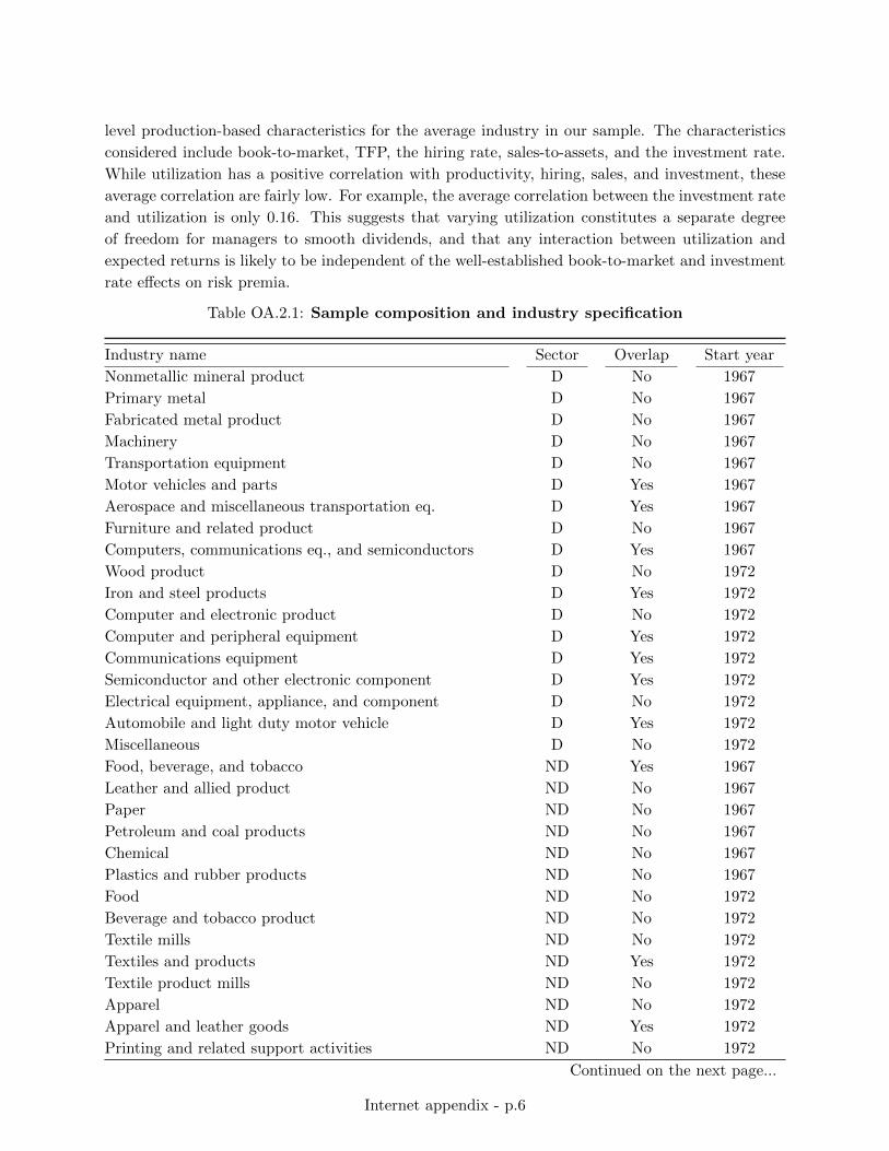
level production-based characteristics for the average industry in our sample. The characteristics

considered include book-to-market, TFP, the hiring rate, sales-to-assets, and the investment rate.

While utilization has a positive correlation with productivity, hiring, sales, and investment, these

average correlation are fairly low. For example, the average correlation between the investment rate

and utilization is only 0.16. This suggests that varying utilization constitutes a separate degree

of freedom for managers to smooth dividends, and that any interaction between utilization and

expected returns is likely to be independent of the well-established book-to-market and investment

rate effects on risk premia.

Table OA.2.1: Sample composition and industry specification

Industry name Sector Overlap Start year

Nonmetallic mineral product D No 1967

Primary metal D No 1967

Fabricated metal product D No 1967

Machinery D No 1967

Transportation equipment D No 1967

Motor vehicles and parts D Yes 1967

Aerospace and miscellaneous transportation eq. D Yes 1967

Furniture and related product D No 1967

Computers, communications eq., and semiconductors D Yes 1967

Wood product D No 1972

Iron and steel products D Yes 1972

Computer and electronic product D No 1972

Computer and peripheral equipment D Yes 1972

Communications equipment D Yes 1972

Semiconductor and other electronic component D Yes 1972

Electrical equipment, appliance, and component D No 1972

Automobile and light duty motor vehicle D Yes 1972

Miscellaneous D No 1972

Food, beverage, and tobacco ND Yes 1967

Leather and allied product ND No 1967

Paper ND No 1967

Petroleum and coal products ND No 1967

Chemical ND No 1967

Plastics and rubber products ND No 1967

Food ND No 1972

Beverage and tobacco product ND No 1972

Textile mills ND No 1972

Textiles and products ND Yes 1972

Textile product mills ND No 1972

Apparel ND No 1972

Apparel and leather goods ND Yes 1972

Printing and related support activities ND No 1972

Continued on the next page...

Internet appendix - p.6

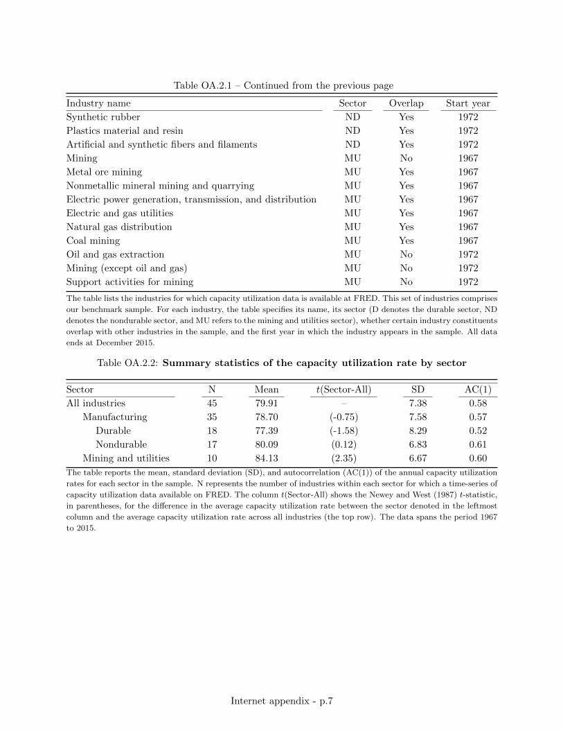
Table OA.2.1 – Continued from the previous page

Industry name Sector Overlap Start year

Synthetic rubber ND Yes 1972

Plastics material and resin ND Yes 1972

Artificial and synthetic fibers and filaments ND Yes 1972

Mining MU No 1967

Metal ore mining MU Yes 1967

Nonmetallic mineral mining and quarrying MU Yes 1967

Electric power generation, transmission, and distribution MU Yes 1967

Electric and gas utilities MU Yes 1967

Natural gas distribution MU Yes 1967

Coal mining MU Yes 1967

Oil and gas extraction MU No 1972

Mining (except oil and gas) MU No 1972

Support activities for mining MU No 1972

The table lists the industries for which capacity utilization data is available at FRED. This set of industries comprises

our benchmark sample. For each industry, the table specifies its name, its sector (D denotes the durable sector, ND

denotes the nondurable sector, and MU refers to the mining and utilities sector), whether certain industry constituents

overlap with other industries in the sample, and the first year in which the industry appears in the sample. All data

ends at December 2015.

Table OA.2.2: Summary statistics of the capacity utilization rate by sector

Sector N Mean t(Sector-All) SD AC(1)

All industries 45 79.91 – 7.38 0.58

Manufacturing 35 78.70 (-0.75) 7.58 0.57

Durable 18 77.39 (-1.58) 8.29 0.52

Nondurable 17 80.09 (0.12) 6.83 0.61

Mining and utilities 10 84.13 (2.35) 6.67 0.60

The table reports the mean, standard deviation (SD), and autocorrelation (AC(1)) of the annual capacity utilization

rates for each sector in the sample. N represents the number of industries within each sector for which a time-series of

capacity utilization data available on FRED. The column t(Sector-All) shows the Newey and West (1987) t-statistic,

in parentheses, for the difference in the average capacity utilization rate between the sector denoted in the leftmost

column and the average capacity utilization rate across all industries (the top row). The data spans the period 1967

to 2015.

Internet appendix - p.7

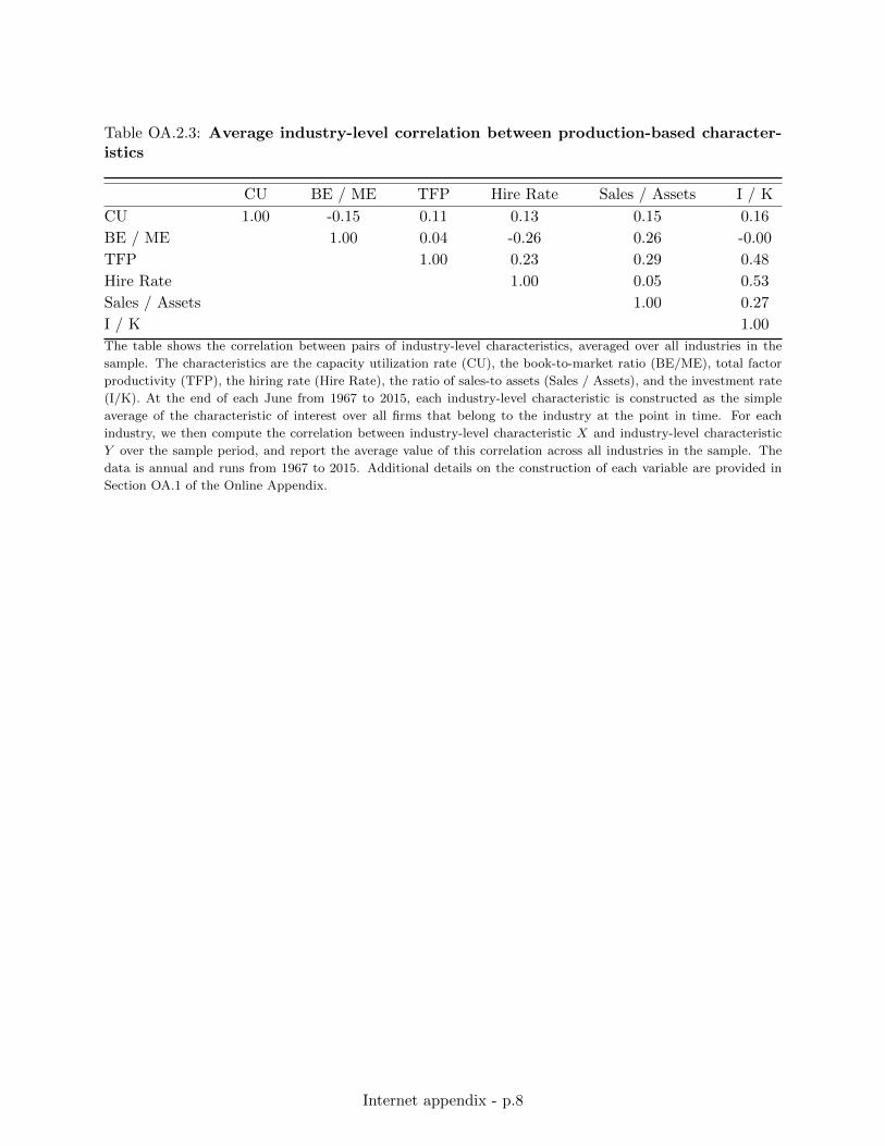
Table OA.2.3: Average industry-level correlation between production-based character-istics

CU BE / ME TFP Hire Rate Sales / Assets I / K

CU 1.00 -0.15 0.11 0.13 0.15 0.16

BE / ME 1.00 0.04 -0.26 0.26 -0.00

TFP 1.00 0.23 0.29 0.48

Hire Rate 1.00 0.05 0.53

Sales / Assets 1.00 0.27

I / K 1.00

The table shows the correlation between pairs of industry-level characteristics, averaged over all industries in the

sample. The characteristics are the capacity utilization rate (CU), the book-to-market ratio (BE/ME), total factor

productivity (TFP), the hiring rate (Hire Rate), the ratio of sales-to assets (Sales / Assets), and the investment rate

(I/K). At the end of each June from 1967 to 2015, each industry-level characteristic is constructed as the simple

average of the characteristic of interest over all firms that belong to the industry at the point in time. For each

industry, we then compute the correlation between industry-level characteristic X and industry-level characteristic

Y over the sample period, and report the average value of this correlation across all industries in the sample. The

data is annual and runs from 1967 to 2015. Additional details on the construction of each variable are provided in

Section OA.1 of the Online Appendix.

Internet appendix - p.8

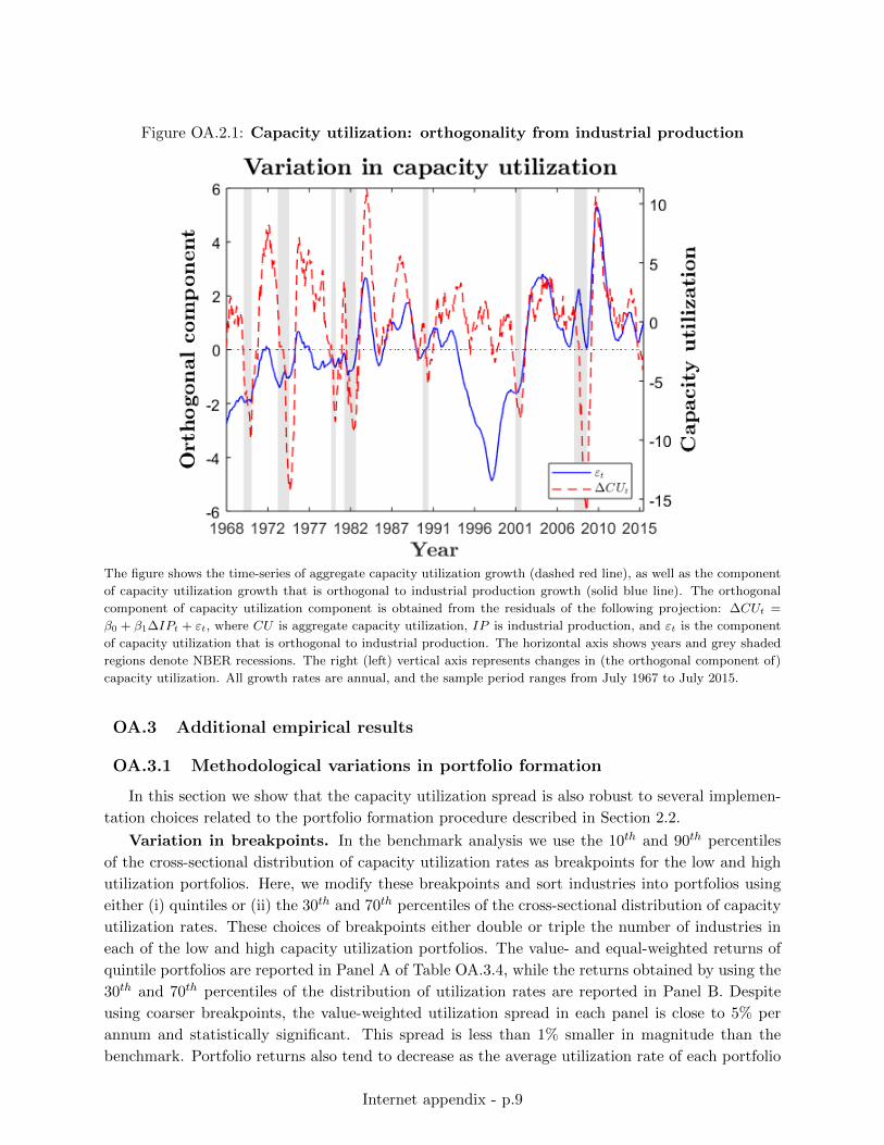
Figure OA.2.1: Capacity utilization: orthogonality from industrial production

The figure shows the time-series of aggregate capacity utilization growth (dashed red line), as well as the component

of capacity utilization growth that is orthogonal to industrial production growth (solid blue line). The orthogonal

component of capacity utilization component is obtained from the residuals of the following projection: ∆CUt =

β0 + β1∆IPt + εt, where CU is aggregate capacity utilization, IP is industrial production, and εt is the component

of capacity utilization that is orthogonal to industrial production. The horizontal axis shows years and grey shaded

regions denote NBER recessions. The right (left) vertical axis represents changes in (the orthogonal component of)

capacity utilization. All growth rates are annual, and the sample period ranges from July 1967 to July 2015.

OA.3 Additional empirical results

OA.3.1 Methodological variations in portfolio formation

In this section we show that the capacity utilization spread is also robust to several implemen-

tation choices related to the portfolio formation procedure described in Section 2.2.

Variation in breakpoints. In the benchmark analysis we use the 10th and 90th percentiles

of the cross-sectional distribution of capacity utilization rates as breakpoints for the low and high

utilization portfolios. Here, we modify these breakpoints and sort industries into portfolios using

either (i) quintiles or (ii) the 30th and 70th percentiles of the cross-sectional distribution of capacity

utilization rates. These choices of breakpoints either double or triple the number of industries in

each of the low and high capacity utilization portfolios. The value- and equal-weighted returns of

quintile portfolios are reported in Panel A of Table OA.3.4, while the returns obtained by using the

30th and 70th percentiles of the distribution of utilization rates are reported in Panel B. Despite

using coarser breakpoints, the value-weighted utilization spread in each panel is close to 5% per

annum and statistically significant. This spread is less than 1% smaller in magnitude than the

benchmark. Portfolio returns also tend to decrease as the average utilization rate of each portfolio

Internet appendix - p.9

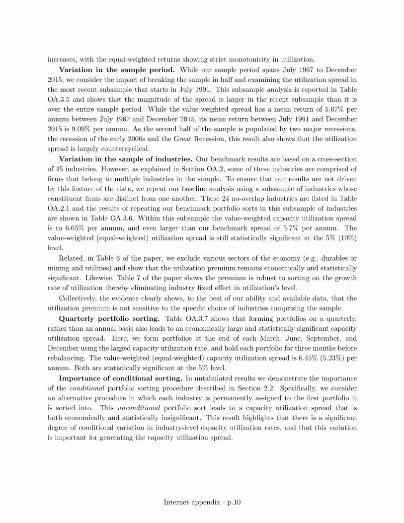
increases, with the equal-weighted returns showing strict monotonicity in utilization.

Variation in the sample period. While our sample period spans July 1967 to December

2015, we consider the impact of breaking the sample in half and examining the utilization spread in

the most recent subsample that starts in July 1991. This subsample analysis is reported in Table

OA.3.5 and shows that the magnitude of the spread is larger in the recent subsample than it is

over the entire sample period. While the value-weighted spread has a mean return of 5.67% per

annum between July 1967 and December 2015, its mean return between July 1991 and December

2015 is 9.09% per annum. As the second half of the sample is populated by two major recessions,

the recession of the early 2000s and the Great Recession, this result also shows that the utilization

spread is largely countercyclical.

Variation in the sample of industries. Our benchmark results are based on a cross-section

of 45 industries. However, as explained in Section OA.2, some of these industries are comprised of

firms that belong to multiple industries in the sample. To ensure that our results are not driven

by this feature of the data, we repeat our baseline analysis using a subsample of industries whose

constituent firms are distinct from one another. These 24 no-overlap industries are listed in Table

OA.2.1 and the results of repeating our benchmark portfolio sorts in this subsample of industries

are shown in Table OA.3.6. Within this subsample the value-weighted capacity utilization spread

is to 6.65% per annum, and even larger than our benchmark spread of 5.7% per annum. The

value-weighted (equal-weighted) utilization spread is still statistically significant at the 5% (10%)

level.

Related, in Table 6 of the paper, we exclude various sectors of the economy (e.g., durables or

mining and utilities) and show that the utilization premium remains economically and statistically

significant. Likewise, Table 7 of the paper shows the premium is robust to sorting on the growth

rate of utilization thereby eliminating industry fixed effect in utilization’s level.

Collectively, the evidence clearly shows, to the best of our ability and available data, that the

utilization premium is not sensitive to the specific choice of industries comprising the sample.

Quarterly portfolio sorting. Table OA.3.7 shows that forming portfolios on a quarterly,

rather than an annual basis also leads to an economically large and statistically significant capacity

utilization spread. Here, we form portfolios at the end of each March, June, September, and

December using the lagged capacity utilization rate, and hold each portfolio for three months before

rebalancing. The value-weighted (equal-weighted) capacity utilization spread is 6.45% (5.23%) per

annum. Both are statistically significant at the 5% level.

Importance of conditional sorting. In untabulated results we demonstrate the importance

of the conditional portfolio sorting procedure described in Section 2.2. Specifically, we consider

an alternative procedure in which each industry is permanently assigned to the first portfolio it

is sorted into. This unconditional portfolio sort leads to a capacity utilization spread that is

both economically and statistically insignificant. This result highlights that there is a significant

degree of conditional variation in industry-level capacity utilization rates, and that this variation

is important for generating the capacity utilization spread.

Internet appendix - p.10

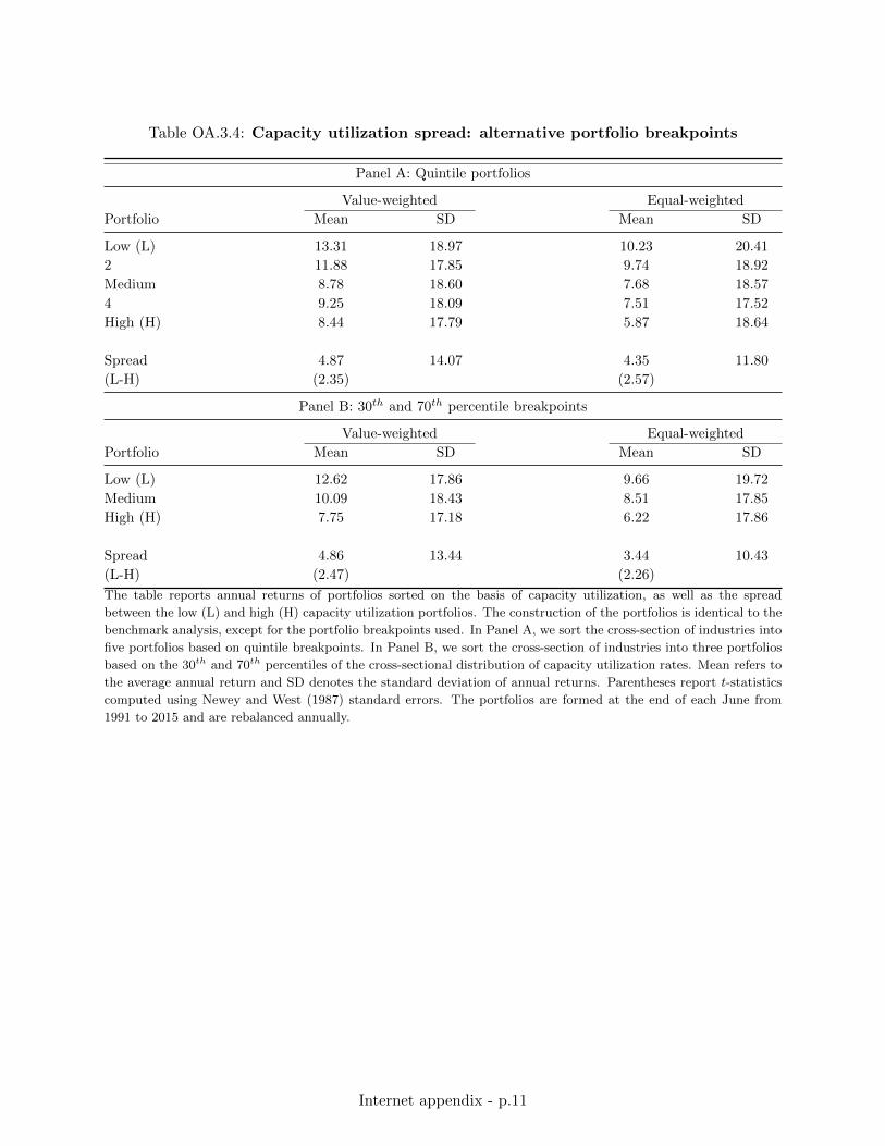
Table OA.3.4: Capacity utilization spread: alternative portfolio breakpoints

Panel A: Quintile portfolios

Value-weighted Equal-weighted

Portfolio Mean SD Mean SD

Low (L) 13.31 18.97 10.23 20.41

2 11.88 17.85 9.74 18.92

Medium 8.78 18.60 7.68 18.57

4 9.25 18.09 7.51 17.52

High (H) 8.44 17.79 5.87 18.64

Spread 4.87 14.07 4.35 11.80

(L-H) (2.35) (2.57)

Panel B: 30th and 70th percentile breakpoints

Value-weighted Equal-weighted

Portfolio Mean SD Mean SD

Low (L) 12.62 17.86 9.66 19.72

Medium 10.09 18.43 8.51 17.85

High (H) 7.75 17.18 6.22 17.86

Spread 4.86 13.44 3.44 10.43

(L-H) (2.47) (2.26)

The table reports annual returns of portfolios sorted on the basis of capacity utilization, as well as the spread

between the low (L) and high (H) capacity utilization portfolios. The construction of the portfolios is identical to the

benchmark analysis, except for the portfolio breakpoints used. In Panel A, we sort the cross-section of industries into

five portfolios based on quintile breakpoints. In Panel B, we sort the cross-section of industries into three portfolios

based on the 30th and 70th percentiles of the cross-sectional distribution of capacity utilization rates. Mean refers to

the average annual return and SD denotes the standard deviation of annual returns. Parentheses report t-statistics

computed using Newey and West (1987) standard errors. The portfolios are formed at the end of each June from

1991 to 2015 and are rebalanced annually.

Internet appendix - p.11

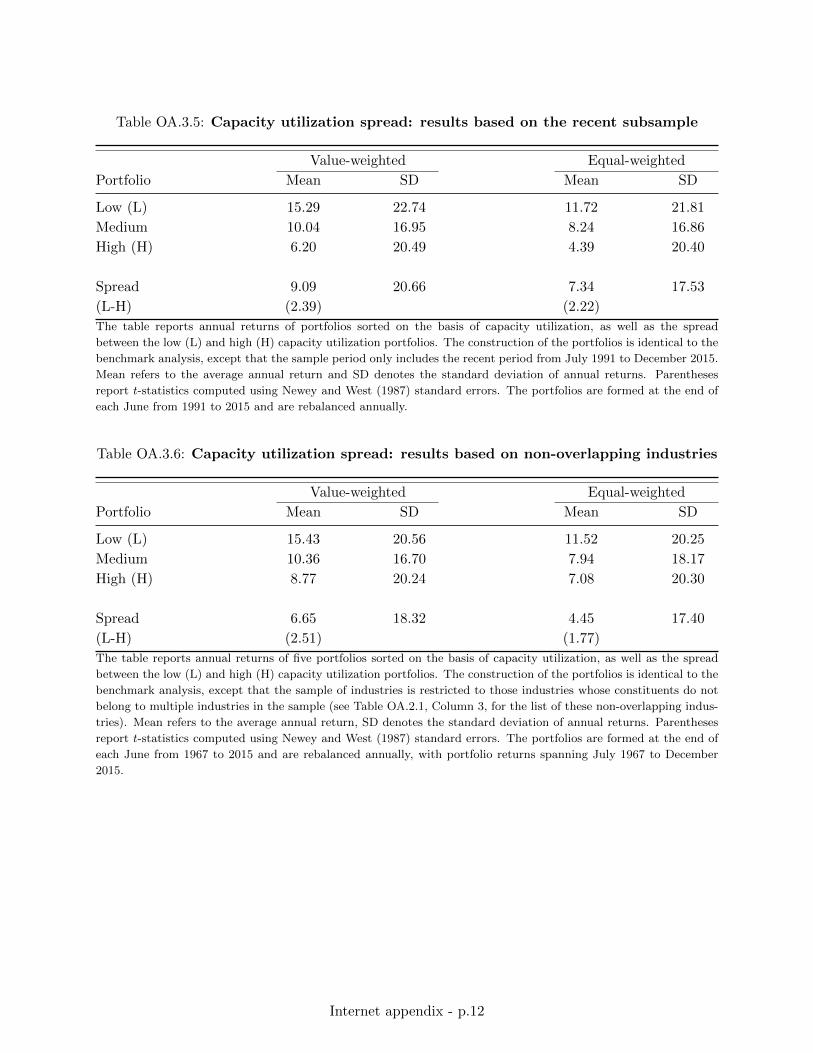
Table OA.3.5: Capacity utilization spread: results based on the recent subsample

Value-weighted Equal-weighted

Portfolio Mean SD Mean SD

Low (L) 15.29 22.74 11.72 21.81

Medium 10.04 16.95 8.24 16.86

High (H) 6.20 20.49 4.39 20.40

Spread 9.09 20.66 7.34 17.53

(L-H) (2.39) (2.22)

The table reports annual returns of portfolios sorted on the basis of capacity utilization, as well as the spread

between the low (L) and high (H) capacity utilization portfolios. The construction of the portfolios is identical to the

benchmark analysis, except that the sample period only includes the recent period from July 1991 to December 2015.

Mean refers to the average annual return and SD denotes the standard deviation of annual returns. Parentheses

report t-statistics computed using Newey and West (1987) standard errors. The portfolios are formed at the end of

each June from 1991 to 2015 and are rebalanced annually.

Table OA.3.6: Capacity utilization spread: results based on non-overlapping industries

Value-weighted Equal-weighted

Portfolio Mean SD Mean SD

Low (L) 15.43 20.56 11.52 20.25

Medium 10.36 16.70 7.94 18.17

High (H) 8.77 20.24 7.08 20.30

Spread 6.65 18.32 4.45 17.40

(L-H) (2.51) (1.77)

The table reports annual returns of five portfolios sorted on the basis of capacity utilization, as well as the spread

between the low (L) and high (H) capacity utilization portfolios. The construction of the portfolios is identical to the

benchmark analysis, except that the sample of industries is restricted to those industries whose constituents do not

belong to multiple industries in the sample (see Table OA.2.1, Column 3, for the list of these non-overlapping indus-

tries). Mean refers to the average annual return, SD denotes the standard deviation of annual returns. Parentheses

report t-statistics computed using Newey and West (1987) standard errors. The portfolios are formed at the end of

each June from 1967 to 2015 and are rebalanced annually, with portfolio returns spanning July 1967 to December

2015.

Internet appendix - p.12

Table OA.3.7: Capacity utilization spread: quarterly portfolio formation

Value-weighted Equal-weighted

Portfolio Mean SD Mean SD

Low (L) 13.66 21.91 10.33 21.52

Medium 10.69 16.65 8.23 17.55

High (H) 7.20 20.48 5.10 21.00

Spread 6.45 18.57 5.23 16.55

(L-H) (2.41) (2.21)

The table reports annual returns of three portfolios sorted on the basis of capacity utilization, as well as the spread

between the low (L) and high (H) capacity utilization portfolios. Here, portfolios are formed at the end of each

March, June, September, and December on the basis of each industry’s lagged capacity utilization rate. Each of these

portfolios is then held for three months before rebalancing. Mean refers to the average annual return, SD denotes

the standard deviation of annual returns. Parentheses report t-statistics computed using Newey and West (1987)

standard errors. The portfolios are formed at the end of each quarter from 1967 to 2015, with portfolio returns

spanning April 1967 to December 2015.

OA.3.2 Conditional CAPM and time-varying betas to aggregate productivity

In this section we show that time-varying exposures to the market (aggregate productivity)

fully absorb the utilization premium.

Conditional CAPM. We estimate the conditional CAPM to show that time variation in risk

exposures are important to reconcile the utilization premium. Here, we estimate the conditional

CAPM following the procedure outlined by Lewellen and Nagel (2006). That is, within each

year of the sample period, we estimate an unconditional CAPM regression that projects each

portfolio’s excess returns on excess market returns. We then compute the time-series average of

the corresponding CAPM alphas and betas. The results, reported in Table OA.3.8, confirm that

a single-factor model is able to explain the utilization premium. Accounting for time-variation

in CAPM betas reduces the economic magnitude of the average CAPM alpha, compared to the

unconditional specification, and renders the alpha statistically insignificant.

Internet appendix - p.13

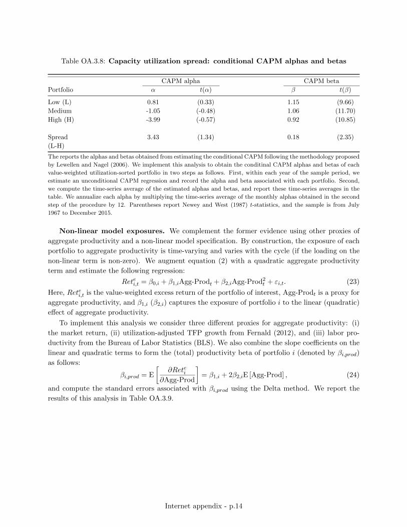
Table OA.3.8: Capacity utilization spread: conditional CAPM alphas and betas

CAPM alpha CAPM beta

Portfolio α t(α) β t(β)

Low (L) 0.81 (0.33) 1.15 (9.66)

Medium -1.05 (-0.48) 1.06 (11.70)

High (H) -3.99 (-0.57) 0.92 (10.85)

Spread 3.43 (1.34) 0.18 (2.35)

(L-H)

The reports the alphas and betas obtained from estimating the conditional CAPM following the methodology proposed

by Lewellen and Nagel (2006). We implement this analysis to obtain the conditinal CAPM alphas and betas of each

value-weighted utilization-sorted portfolio in two steps as follows. First, within each year of the sample period, we

estimate an unconditional CAPM regression and record the alpha and beta associated with each portfolio. Second,

we compute the time-series average of the estimated alphas and betas, and report these time-series averages in the

table. We annualize each alpha by multiplying the time-series average of the monthly alphas obtained in the second

step of the procedure by 12. Parentheses report Newey and West (1987) t-statistics, and the sample is from July

1967 to December 2015.

Non-linear model exposures. We complement the former evidence using other proxies of

aggregate productivity and a non-linear model specification. By construction, the exposure of each

portfolio to aggregate productivity is time-varying and varies with the cycle (if the loading on the

non-linear term is non-zero). We augment equation (2) with a quadratic aggregate productivity

term and estimate the following regression:

Retei,t = β0,i + β1,iAgg-Prodt + β2,iAgg-Prod2t + εi,t. (23)

Here, Retei,t is the value-weighted excess return of the portfolio of interest, Agg-Prodt is a proxy for

aggregate productivity, and β1,i (β2,i) captures the exposure of portfolio i to the linear (quadratic)

effect of aggregate productivity.

To implement this analysis we consider three different proxies for aggregate productivity: (i)

the market return, (ii) utilization-adjusted TFP growth from Fernald (2012), and (iii) labor pro-

ductivity from the Bureau of Labor Statistics (BLS). We also combine the slope coefficients on the

linear and quadratic terms to form the (total) productivity beta of portfolio i (denoted by βi,prod)

as follows:

βi,prod = E

[∂Retei

∂Agg-Prod

]= β1,i + 2β2,iE [Agg-Prod] , (24)

and compute the standard errors associated with βi,prod using the Delta method. We report the

results of this analysis in Table OA.3.9.

Internet appendix - p.14

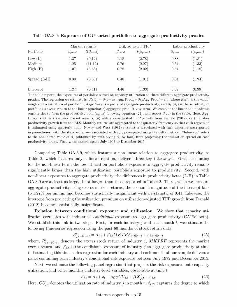
Table OA.3.9: Exposure of CU-sorted portfolios to aggregate productivity proxies

Market returns Util.-adjusted TFP Labor productivity

Portfolio βprod t(βprod) βprod t(βprod) βprod t(βprod)

Low (L) 1.37 (9.12) 1.18 (2.78) 0.88 (1.81)

Medium 1.25 (11.12) 0.76 (2.27) 0.54 (1.33)

High (H) 1.07 (6.53) 0.78 (2.02) 0.54 (1.18)

Spread (L-H) 0.30 (3.53) 0.40 (1.91) 0.34 (1.94)

Intercept 1.27 (0.41) 4.46 (1.33) 3.08 (0.99)

The table reports the exposures of portfolios sorted on capacity utilization to three different aggregate productivity

proxies. The regression we estimate is: Retei,t = β0,i+β1,iAgg-Prodt+β2,iAgg-Prod2t +εi,t, where Retei,t is the value-

weighted excess return of portfolio i, Agg-Proxy is a proxy of aggregate productivity, and β1 (β2) is the sensitivity of

portfolio i’s excess return to the linear (quadratic) aggregate productivity term. We combine the linear and quadratic

sensitivities to form the productivity beta (βprod) following equation (24), and report βprod in the table. Here, Agg-

Proxy is either (i) excess market returns, (ii) utilization-adjusted TFP growth from Fernald (2012), or (iii) labor

productivity growth from the BLS. Monthly returns are aggregated to the quarterly frequency so that each regression

is estimated using quarterly data. Newey and West (1987) t-statistics associated with each exposure are reported

in parentheses, with the standard errors associated with βprod computed using the delta method. “Intercept” refers

to the annualized value of β0 (obtained by multiplying β0 by four) from projecting the utilization spread on each

productivity proxy. Finally, the sample spans July 1967 to December 2015.

Comparing Table OA.3.9, which features a non-linear relation to aggregate productivity, to

Table 2, which features only a linear relation, delivers three key takeaways. First, accounting

for the non-linear term, the low utilization portfolio’s exposure to aggregate productivity remains

significantly larger than the high utilization portfolio’s exposure to productivity. Second, with

non-linear exposures to aggregate productivity, the differences in productivity betas (L-H) in Table

OA.3.9 are at least as large, if not larger, than those reported in Table 2. Third, when we measure

aggregate productivity using excess market returns, the economic magnitude of the intercept falls

to 1.27% per annum and becomes statistically insignificant with a t-statistic of 0.41. Likewise, the

intercept from projecting the utilization premium on utilization-adjusted TFP growth from Fernald

(2012) becomes statistically insignificant.

Relation between conditional exposure and utilization. We show that capacity uti-

lization correlates with industries’ conditional exposure to aggregate productivity (CAPM beta).

We establish this link in two steps. First, for each industry j and each month t, we estimate the

following time-series regression using the past 60 months of stock return data

Rej,t−60→t = αj,t + βj,tMKTRFt−60→t + εj,t−60→t, (25)

where, Rej,t−60→t denotes the excess stock return of industry j, MKTRF represents the market

excess return, and βj,t is the conditional exposure of industry j to aggregate productivity at time

t. Estimating this time-series regression for each industry and each month of our sample delivers a

panel containing each industry’s conditional risk exposure between July 1972 and December 2015.

Next, we estimate the following panel regression that projects the risk exposures onto capacity

utilization, and other monthly industry-level variables, observable at time t

βj,t = αj + δt + βCUCUj,t + βX′j,t + εj,t. (26)

Here, CUj,t denotes the utilization rate of industry j in month t. βCU captures the degree to which

Internet appendix - p.15

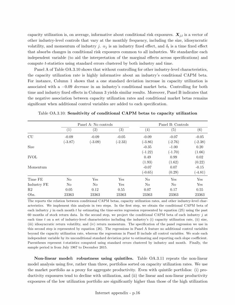
capacity utilization is, on average, informative about conditional risk exposures. Xj,t is a vector of

other industry-level controls that vary at the monthly frequency, including the size, idiosyncratic

volatility, and momentum of industry j. αj is an industry fixed effect, and δt is a time fixed effect

that absorbs changes in conditional risk exposures common to all industries. We standardize each

independent variable (to aid the interpretation of the marginal effects across specifications) and

compute t-statistics using standard errors clustered by both industry and time.

Panel A of Table OA.3.10 shows that without controlling for other industry-level characteristics,

the capacity utilization rate is highly informative about an industry’s conditional CAPM beta.

For instance, Column 1 shows that a one standard deviation increase in capacity utilization is

associated with a −0.09 decrease in an industry’s conditional market beta. Controlling for both

time and industry fixed effects in Column 3 yields similar results. Moreover, Panel B indicates that

the negative association between capacity utilization rates and conditional market betas remains

significant when additional control variables are added to each specification.

Table OA.3.10: Sensitivity of conditional CAPM betas to capacity utilization

Panel A: No controls Panel B: Controls

(1) (2) (3) (4) (5) (6)

CU -0.09 -0.09 -0.05 -0.09 -0.07 -0.05

(-3.87) (-3.09) (-2.33) (-3.86) (-2.76) (-2.38)

Size -0.35 -1.00 0.20

(-1.22) (-1.70) (1.66)

IVOL 0.49 0.99 0.02

(1.93) (1.62) (0.22)

Momentum -0.07 0.07 -0.15

(-0.65) (0.29) (-4.81)

Time FE No Yes Yes No Yes Yes

Industry FE No No Yes No No Yes

R2 0.05 0.12 0.55 0.07 0.17 0.55

Obs. 23363 23363 23363 23363 23363 23363

The reports the relation between conditional CAPM betas, capacity utilization rates, and other industry-level char-

acteristics. We implement this analysis in two steps. In the first step, we obtain the conditional CAPM beta of

each industry j in each month t by estimating the time-series regression represented by equation (25) using the past

60 months of stock return data. In the second step, we project the conditional CAPM beta of each industry j at

each time t on a set of industry-level characteristics including the industry’s (i) capacity utilization rate, (ii) size,

(iii) idiosyncratic return volatility, and (iv) return momentum. The specification of the panel regression we use in

this second step is represented by equation (26). The regressions in Panel A feature no additional control variables

beyond the capacity utilization rate, whereas the regressions in Panel B include all control variables. We scale each

independent variable by its unconditional standard deviation prior to estimating and reporting each slope coefficient.

Parentheses represent t-statistics computed using standard errors clustered by industry and month. Finally, the

sample period is from July 1967 to December 2015.

Non-linear model: robustness using quintiles. Table OA.3.11 repeats the non-linear

model analysis using five, rather than three, portfolios sorted on capacity utilization rates. We use

the market portfolio as a proxy for aggregate productivity. Even with quintile portfolios: (i) pro-

ductivity exposures tend to decline with utilization, and (ii) the linear and non-linear productivity

exposures of the low utilization portfolio are significantly higher than those of the high utilization

Internet appendix - p.16

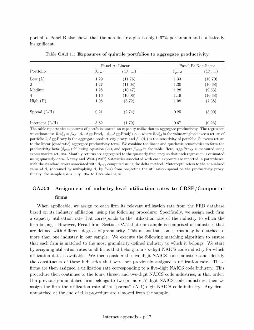
portfolio. Panel B also shows that the non-linear alpha is only 0.67% per annum and statistically

insignificant.

Table OA.3.11: Exposures of quintile portfolios to aggregate productivity

Panel A: Linear Panel B: Non-linear

Portfolio βprod t(βprod) βprod t(βprod)

Low (L) 1.29 (11.76) 1.33 (10.70)

2 1.27 (11.68) 1.30 (10.68)

Medium 1.28 (10.47) 1.28 (9.53)

4 1.16 (10.96) 1.19 (10.38)

High (H) 1.08 (8.72) 1.08 (7.38)

Spread (L-H) 0.21 (2.74) 0.25 (3.00)

Intercept (L-H) 3.82 (1.79) 0.67 (0.26)

The table reports the exposures of portfolios sorted on capacity utilization to aggregate productivity. The regression

we estimate is: Retei,t = β0,i+β1,iAgg-Prodt+β2,iAgg-Prod2t +εi,t, where Retei,t is the value-weighted excess return of

portfolio i, Agg-Proxy is the aggregate productivity proxy, and β1 (β2) is the sensitivity of portfolio i’s excess return

to the linear (quadratic) aggregate productivity term. We combine the linear and quadratic sensitivities to form the

productivity beta (βprod) following equation (24), and report βprod in the table. Here, Agg-Proxy is measured using

excess market returns. Monthly returns are aggregated to the quarterly frequency so that each regression is estimated

using quarterly data. Newey and West (1987) t-statistics associated with each exposure are reported in parentheses,

with the standard errors associated with βprod computed using the delta method. “Intercept” refers to the annualized

value of β0 (obtained by multiplying β0 by four) from projecting the utilization spread on the productivity proxy.

Finally, the sample spans July 1967 to December 2015.

OA.3.3 Assignment of industry-level utilization rates to CRSP/Compustat

firms

When applicable, we assign to each firm its relevant utilization rate from the FRB database

based on its industry affiliation, using the following procedure: Specifically, we assign each firm

a capacity utilization rate that corresponds to the utilization rate of the industry to which the

firm belongs. However, Recall from Section OA.2 that our sample is comprised of industries that

are defined with different degrees of granularity. This means that some firms may be matched to

more than one industry in our sample. We execute the following matching algorithm to ensure

that each firm is matched to the most granularity defined industry to which it belongs. We start

by assigning utilization rates to all firms that belong to a six-digit NAICS code industry for which

utilization data is available. We then consider the five-digit NAICS code industries and identify

the constituents of these industries that were not previously assigned a utilization rate. These

firms are then assigned a utilization rate corresponding to a five-digit NAICS code industry. This

procedure then continues to the four-, three-, and two-digit NAICS code industries, in that order.

If a previously unmatched firm belongs to two or more N -digit NAICS code industries, then we

assign the firm the utilization rate of its “parent” (N -1)-digit NAICS code industry. Any firms

unmatched at the end of this procedure are removed from the sample.

Internet appendix - p.17

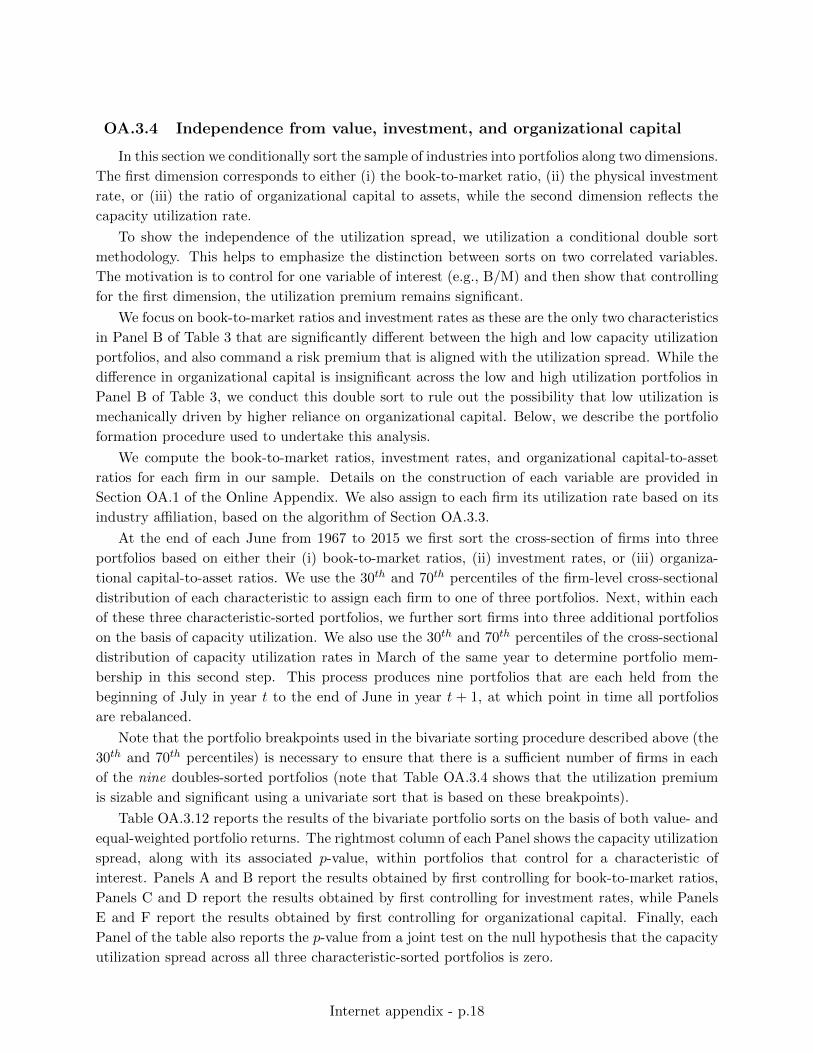
OA.3.4 Independence from value, investment, and organizational capital

In this section we conditionally sort the sample of industries into portfolios along two dimensions.

The first dimension corresponds to either (i) the book-to-market ratio, (ii) the physical investment

rate, or (iii) the ratio of organizational capital to assets, while the second dimension reflects the

capacity utilization rate.

To show the independence of the utilization spread, we utilization a conditional double sort

methodology. This helps to emphasize the distinction between sorts on two correlated variables.

The motivation is to control for one variable of interest (e.g., B/M) and then show that controlling

for the first dimension, the utilization premium remains significant.

We focus on book-to-market ratios and investment rates as these are the only two characteristics

in Panel B of Table 3 that are significantly different between the high and low capacity utilization

portfolios, and also command a risk premium that is aligned with the utilization spread. While the

difference in organizational capital is insignificant across the low and high utilization portfolios in

Panel B of Table 3, we conduct this double sort to rule out the possibility that low utilization is

mechanically driven by higher reliance on organizational capital. Below, we describe the portfolio

formation procedure used to undertake this analysis.

We compute the book-to-market ratios, investment rates, and organizational capital-to-asset

ratios for each firm in our sample. Details on the construction of each variable are provided in

Section OA.1 of the Online Appendix. We also assign to each firm its utilization rate based on its

industry affiliation, based on the algorithm of Section OA.3.3.

At the end of each June from 1967 to 2015 we first sort the cross-section of firms into three

portfolios based on either their (i) book-to-market ratios, (ii) investment rates, or (iii) organiza-

tional capital-to-asset ratios. We use the 30th and 70th percentiles of the firm-level cross-sectional

distribution of each characteristic to assign each firm to one of three portfolios. Next, within each

of these three characteristic-sorted portfolios, we further sort firms into three additional portfolios

on the basis of capacity utilization. We also use the 30th and 70th percentiles of the cross-sectional

distribution of capacity utilization rates in March of the same year to determine portfolio mem-

bership in this second step. This process produces nine portfolios that are each held from the

beginning of July in year t to the end of June in year t + 1, at which point in time all portfolios

are rebalanced.

Note that the portfolio breakpoints used in the bivariate sorting procedure described above (the

30th and 70th percentiles) is necessary to ensure that there is a sufficient number of firms in each

of the nine doubles-sorted portfolios (note that Table OA.3.4 shows that the utilization premium

is sizable and significant using a univariate sort that is based on these breakpoints).

Table OA.3.12 reports the results of the bivariate portfolio sorts on the basis of both value- and

equal-weighted portfolio returns. The rightmost column of each Panel shows the capacity utilization

spread, along with its associated p-value, within portfolios that control for a characteristic of

interest. Panels A and B report the results obtained by first controlling for book-to-market ratios,

Panels C and D report the results obtained by first controlling for investment rates, while Panels

E and F report the results obtained by first controlling for organizational capital. Finally, each

Panel of the table also reports the p-value from a joint test on the null hypothesis that the capacity

utilization spread across all three characteristic-sorted portfolios is zero.

Internet appendix - p.18

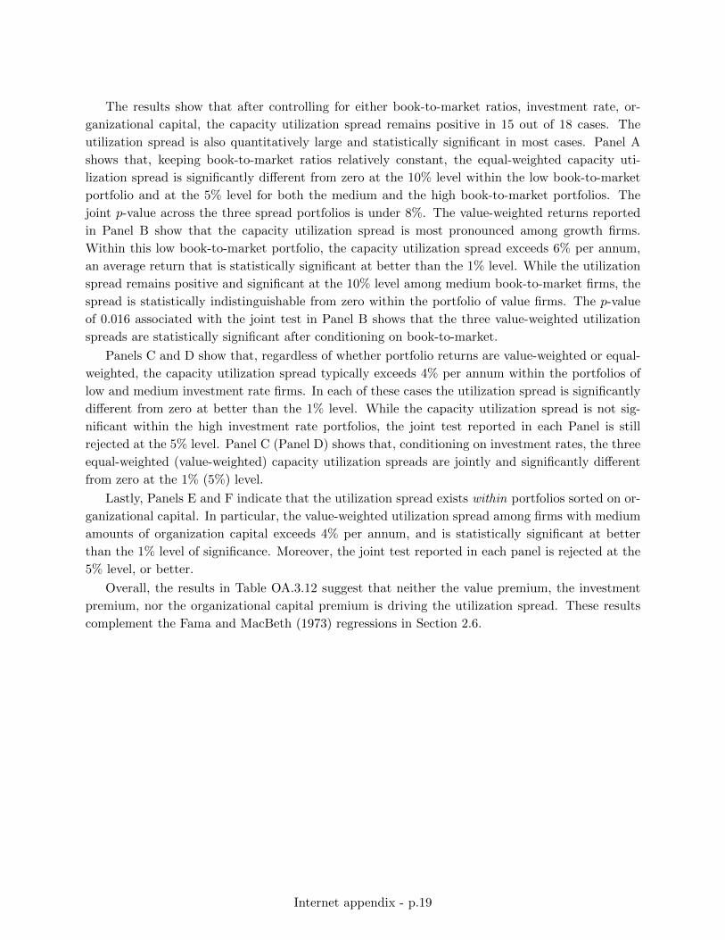
The results show that after controlling for either book-to-market ratios, investment rate, or-

ganizational capital, the capacity utilization spread remains positive in 15 out of 18 cases. The

utilization spread is also quantitatively large and statistically significant in most cases. Panel A

shows that, keeping book-to-market ratios relatively constant, the equal-weighted capacity uti-

lization spread is significantly different from zero at the 10% level within the low book-to-market

portfolio and at the 5% level for both the medium and the high book-to-market portfolios. The

joint p-value across the three spread portfolios is under 8%. The value-weighted returns reported

in Panel B show that the capacity utilization spread is most pronounced among growth firms.

Within this low book-to-market portfolio, the capacity utilization spread exceeds 6% per annum,

an average return that is statistically significant at better than the 1% level. While the utilization

spread remains positive and significant at the 10% level among medium book-to-market firms, the

spread is statistically indistinguishable from zero within the portfolio of value firms. The p-value

of 0.016 associated with the joint test in Panel B shows that the three value-weighted utilization

spreads are statistically significant after conditioning on book-to-market.

Panels C and D show that, regardless of whether portfolio returns are value-weighted or equal-

weighted, the capacity utilization spread typically exceeds 4% per annum within the portfolios of

low and medium investment rate firms. In each of these cases the utilization spread is significantly

different from zero at better than the 1% level. While the capacity utilization spread is not sig-

nificant within the high investment rate portfolios, the joint test reported in each Panel is still

rejected at the 5% level. Panel C (Panel D) shows that, conditioning on investment rates, the three

equal-weighted (value-weighted) capacity utilization spreads are jointly and significantly different

from zero at the 1% (5%) level.

Lastly, Panels E and F indicate that the utilization spread exists within portfolios sorted on or-

ganizational capital. In particular, the value-weighted utilization spread among firms with medium

amounts of organization capital exceeds 4% per annum, and is statistically significant at better

than the 1% level of significance. Moreover, the joint test reported in each panel is rejected at the

5% level, or better.

Overall, the results in Table OA.3.12 suggest that neither the value premium, the investment

premium, nor the organizational capital premium is driving the utilization spread. These results

complement the Fama and MacBeth (1973) regressions in Section 2.6.

Internet appendix - p.19

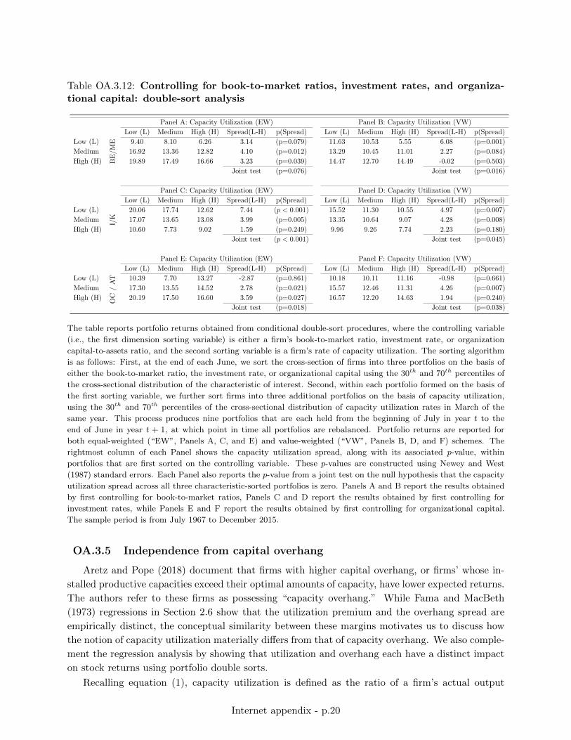
Table OA.3.12: Controlling for book-to-market ratios, investment rates, and organiza-tional capital: double-sort analysis

Panel A: Capacity Utilization (EW) Panel B: Capacity Utilization (VW)

Low (L) Medium High (H) Spread(L-H) p(Spread) Low (L) Medium High (H) Spread(L-H) p(Spread)

Low (L)

BE

/ME 9.40 8.10 6.26 3.14 (p=0.079) 11.63 10.53 5.55 6.08 (p=0.001)

Medium 16.92 13.36 12.82 4.10 (p=0.012) 13.29 10.45 11.01 2.27 (p=0.084)

High (H) 19.89 17.49 16.66 3.23 (p=0.039) 14.47 12.70 14.49 -0.02 (p=0.503)

Joint test (p=0.076) Joint test (p=0.016)

Panel C: Capacity Utilization (EW) Panel D: Capacity Utilization (VW)

Low (L) Medium High (H) Spread(L-H) p(Spread) Low (L) Medium High (H) Spread(L-H) p(Spread)

Low (L)

I/K

20.06 17.74 12.62 7.44 (p < 0.001) 15.52 11.30 10.55 4.97 (p=0.007)

Medium 17.07 13.65 13.08 3.99 (p=0.005) 13.35 10.64 9.07 4.28 (p=0.008)

High (H) 10.60 7.73 9.02 1.59 (p=0.249) 9.96 9.26 7.74 2.23 (p=0.180)

Joint test (p < 0.001) Joint test (p=0.045)

Panel E: Capacity Utilization (EW) Panel F: Capacity Utilization (VW)

Low (L) Medium High (H) Spread(L-H) p(Spread) Low (L) Medium High (H) Spread(L-H) p(Spread)

Low (L)

OC

/A

T 10.39 7.70 13.27 -2.87 (p=0.861) 10.18 10.11 11.16 -0.98 (p=0.661)

Medium 17.30 13.55 14.52 2.78 (p=0.021) 15.57 12.46 11.31 4.26 (p=0.007)

High (H) 20.19 17.50 16.60 3.59 (p=0.027) 16.57 12.20 14.63 1.94 (p=0.240)

Joint test (p=0.018) Joint test (p=0.038)

The table reports portfolio returns obtained from conditional double-sort procedures, where the controlling variable

(i.e., the first dimension sorting variable) is either a firm’s book-to-market ratio, investment rate, or organization

capital-to-assets ratio, and the second sorting variable is a firm’s rate of capacity utilization. The sorting algorithm

is as follows: First, at the end of each June, we sort the cross-section of firms into three portfolios on the basis of

either the book-to-market ratio, the investment rate, or organizational capital using the 30th and 70th percentiles of

the cross-sectional distribution of the characteristic of interest. Second, within each portfolio formed on the basis of

the first sorting variable, we further sort firms into three additional portfolios on the basis of capacity utilization,

using the 30th and 70th percentiles of the cross-sectional distribution of capacity utilization rates in March of the

same year. This process produces nine portfolios that are each held from the beginning of July in year t to the

end of June in year t + 1, at which point in time all portfolios are rebalanced. Portfolio returns are reported for

both equal-weighted (“EW”, Panels A, C, and E) and value-weighted (“VW”, Panels B, D, and F) schemes. The

rightmost column of each Panel shows the capacity utilization spread, along with its associated p-value, within

portfolios that are first sorted on the controlling variable. These p-values are constructed using Newey and West

(1987) standard errors. Each Panel also reports the p-value from a joint test on the null hypothesis that the capacity

utilization spread across all three characteristic-sorted portfolios is zero. Panels A and B report the results obtained

by first controlling for book-to-market ratios, Panels C and D report the results obtained by first controlling for

investment rates, while Panels E and F report the results obtained by first controlling for organizational capital.

The sample period is from July 1967 to December 2015.

OA.3.5 Independence from capital overhang

Aretz and Pope (2018) document that firms with higher capital overhang, or firms’ whose in-

stalled productive capacities exceed their optimal amounts of capacity, have lower expected returns.

The authors refer to these firms as possessing “capacity overhang.” While Fama and MacBeth

(1973) regressions in Section 2.6 show that the utilization premium and the overhang spread are

empirically distinct, the conceptual similarity between these margins motivates us to discuss how

the notion of capacity utilization materially differs from that of capacity overhang. We also comple-

ment the regression analysis by showing that utilization and overhang each have a distinct impact

on stock returns using portfolio double sorts.

Recalling equation (1), capacity utilization is defined as the ratio of a firm’s actual output

Internet appendix - p.20

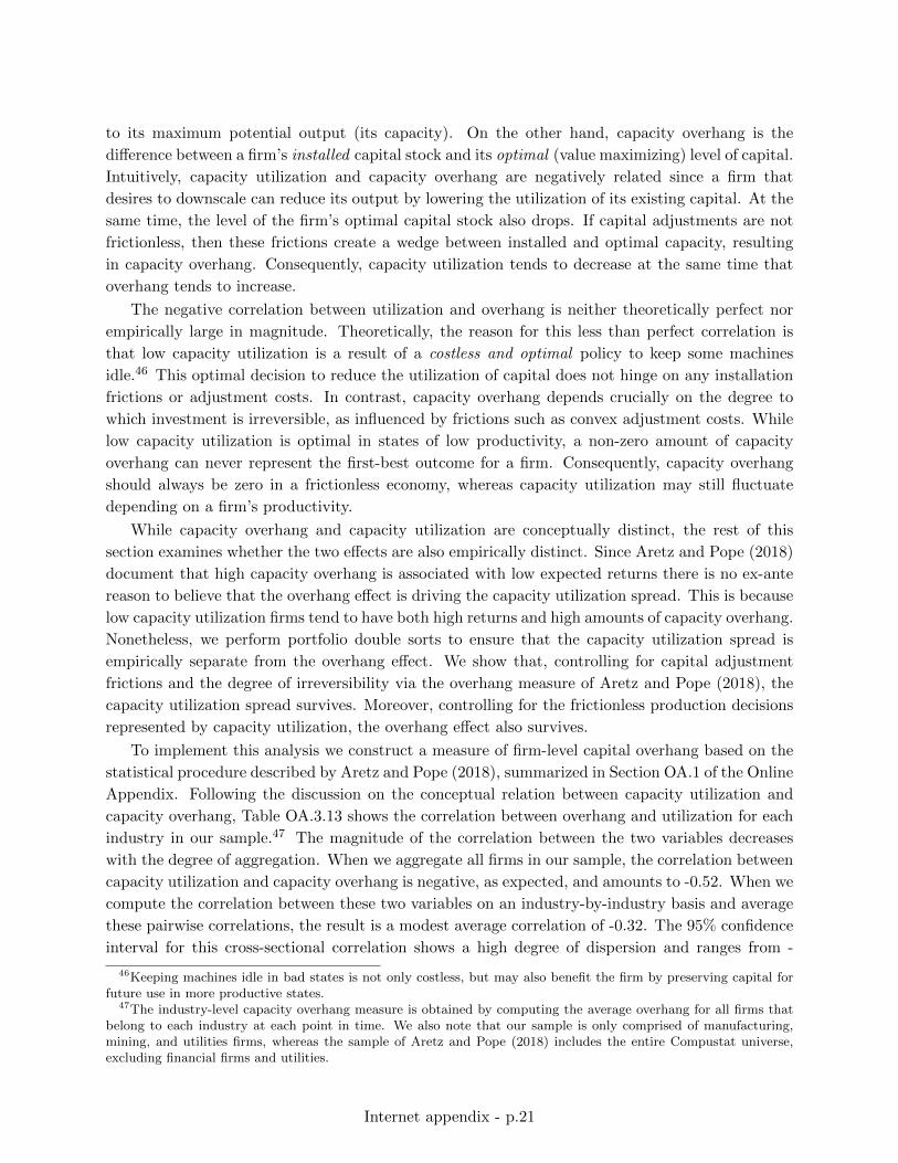
to its maximum potential output (its capacity). On the other hand, capacity overhang is the

difference between a firm’s installed capital stock and its optimal (value maximizing) level of capital.

Intuitively, capacity utilization and capacity overhang are negatively related since a firm that

desires to downscale can reduce its output by lowering the utilization of its existing capital. At the

same time, the level of the firm’s optimal capital stock also drops. If capital adjustments are not

frictionless, then these frictions create a wedge between installed and optimal capacity, resulting

in capacity overhang. Consequently, capacity utilization tends to decrease at the same time that

overhang tends to increase.

The negative correlation between utilization and overhang is neither theoretically perfect nor

empirically large in magnitude. Theoretically, the reason for this less than perfect correlation is

that low capacity utilization is a result of a costless and optimal policy to keep some machines

idle.46 This optimal decision to reduce the utilization of capital does not hinge on any installation

frictions or adjustment costs. In contrast, capacity overhang depends crucially on the degree to

which investment is irreversible, as influenced by frictions such as convex adjustment costs. While

low capacity utilization is optimal in states of low productivity, a non-zero amount of capacity

overhang can never represent the first-best outcome for a firm. Consequently, capacity overhang

should always be zero in a frictionless economy, whereas capacity utilization may still fluctuate

depending on a firm’s productivity.

While capacity overhang and capacity utilization are conceptually distinct, the rest of this

section examines whether the two effects are also empirically distinct. Since Aretz and Pope (2018)

document that high capacity overhang is associated with low expected returns there is no ex-ante

reason to believe that the overhang effect is driving the capacity utilization spread. This is because

low capacity utilization firms tend to have both high returns and high amounts of capacity overhang.

Nonetheless, we perform portfolio double sorts to ensure that the capacity utilization spread is

empirically separate from the overhang effect. We show that, controlling for capital adjustment

frictions and the degree of irreversibility via the overhang measure of Aretz and Pope (2018), the

capacity utilization spread survives. Moreover, controlling for the frictionless production decisions

represented by capacity utilization, the overhang effect also survives.

To implement this analysis we construct a measure of firm-level capital overhang based on the

statistical procedure described by Aretz and Pope (2018), summarized in Section OA.1 of the Online

Appendix. Following the discussion on the conceptual relation between capacity utilization and

capacity overhang, Table OA.3.13 shows the correlation between overhang and utilization for each

industry in our sample.47 The magnitude of the correlation between the two variables decreases

with the degree of aggregation. When we aggregate all firms in our sample, the correlation between

capacity utilization and capacity overhang is negative, as expected, and amounts to -0.52. When we

compute the correlation between these two variables on an industry-by-industry basis and average

these pairwise correlations, the result is a modest average correlation of -0.32. The 95% confidence

interval for this cross-sectional correlation shows a high degree of dispersion and ranges from -

46Keeping machines idle in bad states is not only costless, but may also benefit the firm by preserving capital forfuture use in more productive states.

47The industry-level capacity overhang measure is obtained by computing the average overhang for all firms thatbelong to each industry at each point in time. We also note that our sample is only comprised of manufacturing,mining, and utilities firms, whereas the sample of Aretz and Pope (2018) includes the entire Compustat universe,excluding financial firms and utilities.

Internet appendix - p.21

0.71 to 0.11. Panel C of this table reports that the average firm-level correlation drops to -0.11,

and shows that this correlation becomes even more dispersed in the cross-section of firms. These

results collectively highlight the fact that while capacity utilization and overhang are conceptually

negatively related, the empirical correlation between these two variables is low.

Table OA.3.14 reports the results of performing portfolio double sorts along the dimensions of

capacity utilization and capacity overhang using the conditional double-sort analysis as described

in Section OA.3.4. Panel A shows the average annual capacity utilization spread within three

capacity overhang sorted portfolios when all returns are equal-weighted. The capacity utilization

spread is positive and statistically significant within each overhang portfolio. The utilization spread

is also jointly significant across all three overhang portfolios. Panel B shows that the results are

similar when returns are value-weighted. Panels C and D report that the results are largely similar

after changing the order of the sorts. Controlling for capacity utilization, the joint tests in Panels

C and D show that the capacity overhang spread is positive and statistically significant on an

equal-weighted basis, but is insignificant on a value-weighted basis.

Internet appendix - p.22

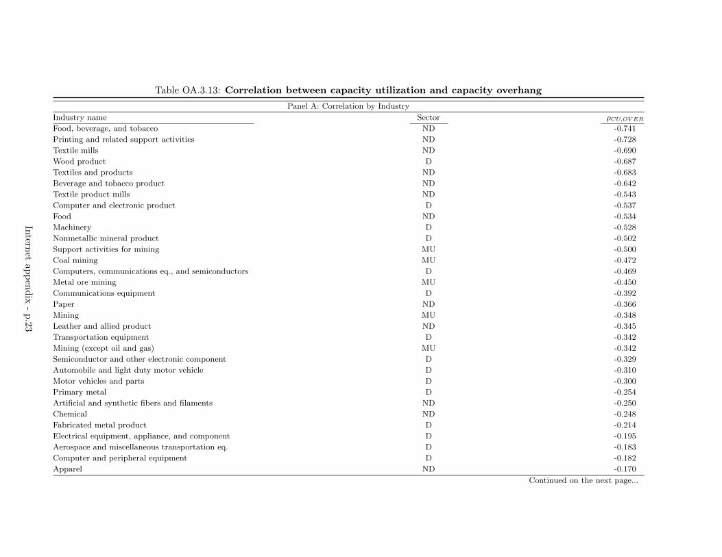
Table OA.3.13: Correlation between capacity utilization and capacity overhang

Panel A: Correlation by Industry

Industry name Sector ρCU,OV ERFood, beverage, and tobacco ND -0.741

Printing and related support activities ND -0.728

Textile mills ND -0.690

Wood product D -0.687

Textiles and products ND -0.683

Beverage and tobacco product ND -0.642

Textile product mills ND -0.543

Computer and electronic product D -0.537

Food ND -0.534

Machinery D -0.528

Nonmetallic mineral product D -0.502

Support activities for mining MU -0.500

Coal mining MU -0.472

Computers, communications eq., and semiconductors D -0.469

Metal ore mining MU -0.450

Communications equipment D -0.392

Paper ND -0.366

Mining MU -0.348

Leather and allied product ND -0.345

Transportation equipment D -0.342

Mining (except oil and gas) MU -0.342

Semiconductor and other electronic component D -0.329

Automobile and light duty motor vehicle D -0.310

Motor vehicles and parts D -0.300

Primary metal D -0.254

Artificial and synthetic fibers and filaments ND -0.250

Chemical ND -0.248

Fabricated metal product D -0.214

Electrical equipment, appliance, and component D -0.195

Aerospace and miscellaneous transportation eq. D -0.183

Computer and peripheral equipment D -0.182

Apparel ND -0.170

Continued on the next page...

Intern

etap

pen

dix

-p

.23

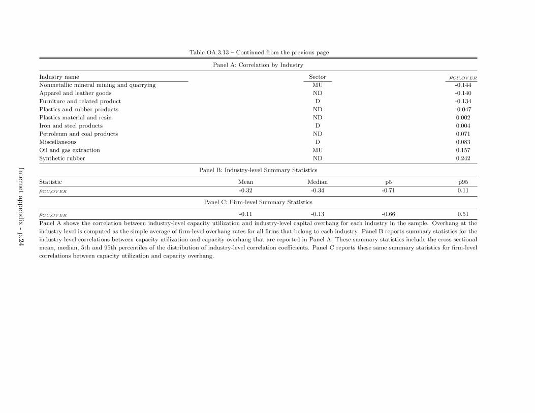
Table OA.3.13 – Continued from the previous page

Panel A: Correlation by Industry

Industry name Sector ρCU,OV ERNonmetallic mineral mining and quarrying MU -0.144

Apparel and leather goods ND -0.140

Furniture and related product D -0.134

Plastics and rubber products ND -0.047

Plastics material and resin ND 0.002

Iron and steel products D 0.004

Petroleum and coal products ND 0.071

Miscellaneous D 0.083

Oil and gas extraction MU 0.157

Synthetic rubber ND 0.242

Panel B: Industry-level Summary Statistics

Statistic Mean Median p5 p95

ρCU,OV ER -0.32 -0.34 -0.71 0.11

Panel C: Firm-level Summary Statistics

ρCU,OV ER -0.11 -0.13 -0.66 0.51

Panel A shows the correlation between industry-level capacity utilization and industry-level capital overhang for each industry in the sample. Overhang at the

industry level is computed as the simple average of firm-level overhang rates for all firms that belong to each industry. Panel B reports summary statistics for the

industry-level correlations between capacity utilization and capacity overhang that are reported in Panel A. These summary statistics include the cross-sectional

mean, median, 5th and 95th percentiles of the distribution of industry-level correlation coefficients. Panel C reports these same summary statistics for firm-level

correlations between capacity utilization and capacity overhang.

Intern

etap

pen

dix

-p

.24

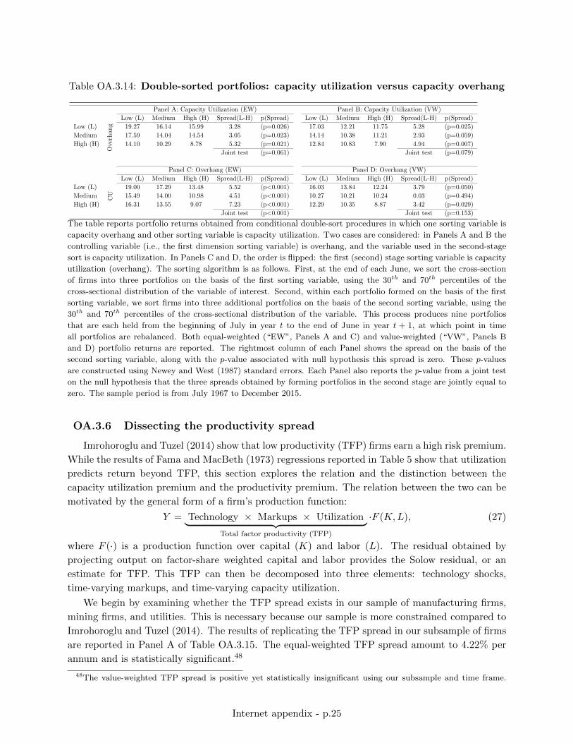
Table OA.3.14: Double-sorted portfolios: capacity utilization versus capacity overhang

Panel A: Capacity Utilization (EW) Panel B: Capacity Utilization (VW)

Low (L) Medium High (H) Spread(L-H) p(Spread) Low (L) Medium High (H) Spread(L-H) p(Spread)

Low (L)

Ove

rhan

g 19.27 16.14 15.99 3.28 (p=0.026) 17.03 12.21 11.75 5.28 (p=0.025)

Medium 17.59 14.04 14.54 3.05 (p=0.023) 14.14 10.38 11.21 2.93 (p=0.059)

High (H) 14.10 10.29 8.78 5.32 (p=0.021) 12.84 10.83 7.90 4.94 (p=0.007)

Joint test (p=0.061) Joint test (p=0.079)

Panel C: Overhang (EW) Panel D: Overhang (VW)

Low (L) Medium High (H) Spread(L-H) p(Spread) Low (L) Medium High (H) Spread(L-H) p(Spread)

Low (L)

CU

19.00 17.29 13.48 5.52 (p<0.001) 16.03 13.84 12.24 3.79 (p=0.050)

Medium 15.49 14.00 10.98 4.51 (p<0.001) 10.27 10.21 10.24 0.03 (p=0.494)

High (H) 16.31 13.55 9.07 7.23 (p<0.001) 12.29 10.35 8.87 3.42 (p=0.029)

Joint test (p<0.001) Joint test (p=0.153)

The table reports portfolio returns obtained from conditional double-sort procedures in which one sorting variable is

capacity overhang and other sorting variable is capacity utilization. Two cases are considered: in Panels A and B the

controlling variable (i.e., the first dimension sorting variable) is overhang, and the variable used in the second-stage

sort is capacity utilization. In Panels C and D, the order is flipped: the first (second) stage sorting variable is capacity

utilization (overhang). The sorting algorithm is as follows. First, at the end of each June, we sort the cross-section

of firms into three portfolios on the basis of the first sorting variable, using the 30th and 70th percentiles of the

cross-sectional distribution of the variable of interest. Second, within each portfolio formed on the basis of the first

sorting variable, we sort firms into three additional portfolios on the basis of the second sorting variable, using the

30th and 70th percentiles of the cross-sectional distribution of the variable. This process produces nine portfolios

that are each held from the beginning of July in year t to the end of June in year t + 1, at which point in time

all portfolios are rebalanced. Both equal-weighted (“EW”, Panels A and C) and value-weighted (“VW”, Panels B

and D) portfolio returns are reported. The rightmost column of each Panel shows the spread on the basis of the

second sorting variable, along with the p-value associated with null hypothesis this spread is zero. These p-values

are constructed using Newey and West (1987) standard errors. Each Panel also reports the p-value from a joint test

on the null hypothesis that the three spreads obtained by forming portfolios in the second stage are jointly equal to

zero. The sample period is from July 1967 to December 2015.

OA.3.6 Dissecting the productivity spread

Imrohoroglu and Tuzel (2014) show that low productivity (TFP) firms earn a high risk premium.

While the results of Fama and MacBeth (1973) regressions reported in Table 5 show that utilization

predicts return beyond TFP, this section explores the relation and the distinction between the

capacity utilization premium and the productivity premium. The relation between the two can be

motivated by the general form of a firm’s production function:

Y = Technology × Markups × Utilization︸ ︷︷ ︸Total factor productivity (TFP)

·F (K,L), (27)

where F (·) is a production function over capital (K) and labor (L). The residual obtained by

projecting output on factor-share weighted capital and labor provides the Solow residual, or an

estimate for TFP. This TFP can then be decomposed into three elements: technology shocks,

time-varying markups, and time-varying capacity utilization.

We begin by examining whether the TFP spread exists in our sample of manufacturing firms,

mining firms, and utilities. This is necessary because our sample is more constrained compared to

Imrohoroglu and Tuzel (2014). The results of replicating the TFP spread in our subsample of firms

are reported in Panel A of Table OA.3.15. The equal-weighted TFP spread amount to 4.22% per

annum and is statistically significant.48

48The value-weighted TFP spread is positive yet statistically insignificant using our subsample and time frame.

Internet appendix - p.25

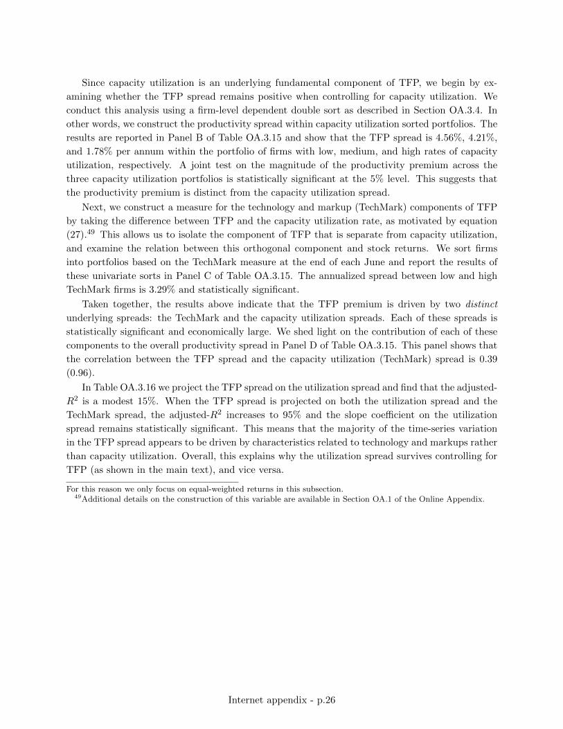
Since capacity utilization is an underlying fundamental component of TFP, we begin by ex-

amining whether the TFP spread remains positive when controlling for capacity utilization. We

conduct this analysis using a firm-level dependent double sort as described in Section OA.3.4. In

other words, we construct the productivity spread within capacity utilization sorted portfolios. The

results are reported in Panel B of Table OA.3.15 and show that the TFP spread is 4.56%, 4.21%,

and 1.78% per annum within the portfolio of firms with low, medium, and high rates of capacity

utilization, respectively. A joint test on the magnitude of the productivity premium across the

three capacity utilization portfolios is statistically significant at the 5% level. This suggests that

the productivity premium is distinct from the capacity utilization spread.

Next, we construct a measure for the technology and markup (TechMark) components of TFP

by taking the difference between TFP and the capacity utilization rate, as motivated by equation

(27).49 This allows us to isolate the component of TFP that is separate from capacity utilization,

and examine the relation between this orthogonal component and stock returns. We sort firms

into portfolios based on the TechMark measure at the end of each June and report the results of

these univariate sorts in Panel C of Table OA.3.15. The annualized spread between low and high

TechMark firms is 3.29% and statistically significant.

Taken together, the results above indicate that the TFP premium is driven by two distinct

underlying spreads: the TechMark and the capacity utilization spreads. Each of these spreads is

statistically significant and economically large. We shed light on the contribution of each of these

components to the overall productivity spread in Panel D of Table OA.3.15. This panel shows that

the correlation between the TFP spread and the capacity utilization (TechMark) spread is 0.39

(0.96).

In Table OA.3.16 we project the TFP spread on the utilization spread and find that the adjusted-

R2 is a modest 15%. When the TFP spread is projected on both the utilization spread and the

TechMark spread, the adjusted-R2 increases to 95% and the slope coefficient on the utilization

spread remains statistically significant. This means that the majority of the time-series variation

in the TFP spread appears to be driven by characteristics related to technology and markups rather

than capacity utilization. Overall, this explains why the utilization spread survives controlling for

TFP (as shown in the main text), and vice versa.

For this reason we only focus on equal-weighted returns in this subsection.49Additional details on the construction of this variable are available in Section OA.1 of the Online Appendix.

Internet appendix - p.26

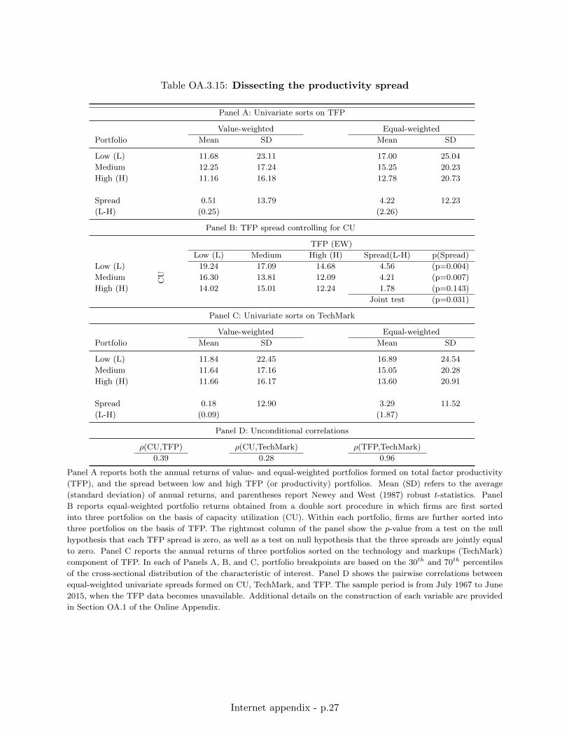
Table OA.3.15: Dissecting the productivity spread

Panel A: Univariate sorts on TFP

Value-weighted Equal-weighted

Portfolio Mean SD Mean SD

Low (L) 11.68 23.11 17.00 25.04

Medium 12.25 17.24 15.25 20.23

High (H) 11.16 16.18 12.78 20.73

Spread 0.51 13.79 4.22 12.23

(L-H) (0.25) (2.26)

Panel B: TFP spread controlling for CU

TFP (EW)

Low (L) Medium High (H) Spread(L-H) p(Spread)

Low (L)

CU

19.24 17.09 14.68 4.56 (p=0.004)

Medium 16.30 13.81 12.09 4.21 (p=0.007)

High (H) 14.02 15.01 12.24 1.78 (p=0.143)

Joint test (p=0.031)

Panel C: Univariate sorts on TechMark

Value-weighted Equal-weighted

Portfolio Mean SD Mean SD

Low (L) 11.84 22.45 16.89 24.54

Medium 11.64 17.16 15.05 20.28

High (H) 11.66 16.17 13.60 20.91

Spread 0.18 12.90 3.29 11.52

(L-H) (0.09) (1.87)

Panel D: Unconditional correlations

ρ(CU,TFP) ρ(CU,TechMark) ρ(TFP,TechMark)

0.39 0.28 0.96

Panel A reports both the annual returns of value- and equal-weighted portfolios formed on total factor productivity

(TFP), and the spread between low and high TFP (or productivity) portfolios. Mean (SD) refers to the average

(standard deviation) of annual returns, and parentheses report Newey and West (1987) robust t-statistics. Panel

B reports equal-weighted portfolio returns obtained from a double sort procedure in which firms are first sorted

into three portfolios on the basis of capacity utilization (CU). Within each portfolio, firms are further sorted into

three portfolios on the basis of TFP. The rightmost column of the panel show the p-value from a test on the null

hypothesis that each TFP spread is zero, as well as a test on null hypothesis that the three spreads are jointly equal

to zero. Panel C reports the annual returns of three portfolios sorted on the technology and markups (TechMark)

component of TFP. In each of Panels A, B, and C, portfolio breakpoints are based on the 30th and 70th percentiles

of the cross-sectional distribution of the characteristic of interest. Panel D shows the pairwise correlations between

equal-weighted univariate spreads formed on CU, TechMark, and TFP. The sample period is from July 1967 to June

2015, when the TFP data becomes unavailable. Additional details on the construction of each variable are provided

in Section OA.1 of the Online Appendix.

Internet appendix - p.27

Table OA.3.16: Projections of the TFP spread on the utilization spread

(1) (2)

β0 2.50 0.41

(1.49) (0.98)

βCU 4.34 1.43

(8.99) (6.38)

βTFP⊥ 11.82

(86.99)

R2 0.152 0.945

Panel A reports the slope coefficients from the following regression: SpreadTFP,t = β0 + βCUSpreadCU,t + εTFP,t,

where SpreadTFP,t is the productivity spread and SpreadCU,t is the utilization spread. Panel B report the coeffi-

cients of the following projection: SpreadTFP,t = β0 + βCUSpreadCU,t + βTFP⊥SpreadTechMark,t + εTFP,t, where

SpreadTechMark,t is the Technology/markup spread. Portfolios are formed annually, at the end of each June, fol-

lowing our benchmark portfolio formation procedure, and returns range from July 1967 to June 2015. t-statistics,

reported in parentheses, are computed using Newey and West (1987) standard errors.

OA.3.7 Robustness: firm-level capacity utilization

For robustness, we construct a proxy for the unobservable capacity utilization rate at the firm-

level. First, for each industry, we project the utilization rate of industry j at time t (CUj,t) on salient

industry-level production-related characteristics, contained in the vector Xj,t. For the dependent

variable, CUj,t, we use either the raw industry utilization or industry-demeaned utilization rate.

The latter approach ensures that the fitted value of this projection is not affected by fixed differences

in average utilization across industries. The choice of Xj,t is motivated by the model in Section

3. We use the logarithms of size and book-to-market, the investment-to-capital ratio, IVOL, and

TFP.50 The regression is

CUj,t = βj,0 + βjXj,t + εj,t (28)

By estimating this projection separately for each industry, the relation between utilization and the

characteristics, as measured by βj , is specific to industry j. The average R2 of this projection across

industries is sizable at 33%, suggesting that the regressors well-span utilization at the industry level.

Second, the proxy for the utilization rate of a firm i that belongs to industry j at time t

(denoted CU i,j,t) is obtained by combining the estimated slope coefficients for industry j, obtained

via equation (28), with the observable characteristics of firm i, denoted Xi,j,t,

CU i,j,t = βj,0 + βjXi,j,t. (29)

This procedure allows the utilization proxy to vary between firms within the same industry. We

use the firm-level utilization proxy to sort firms into portfolios as per Section 2.2, and report the

results in Table OA.3.17.

50Our empirical analysis shows that utilization affects the exposure of firms to aggregate productivity. Consequently,for Xj,t we choose firm-level variables that are known to also correlate with firms’ exposure to this factor. Inparticular, Zhang (2005) shows that aggregate productivity exposure interacts with book-to-market and investment.Imrohoroglu and Tuzel (2014) establish the relation between firm-level TFP and aggregate productivty. Ai andKiku (2016) document that idiosyncratic volatility serves as proxy for underlying growth options, whose riskinessdepends on aggregate consumption. Importantly, in untabulated results we verify that our findings are robust toeither removing particular characteristics (e.g., IVOL) or adding additional characteristics (e.g., hiring rates).

Internet appendix - p.28

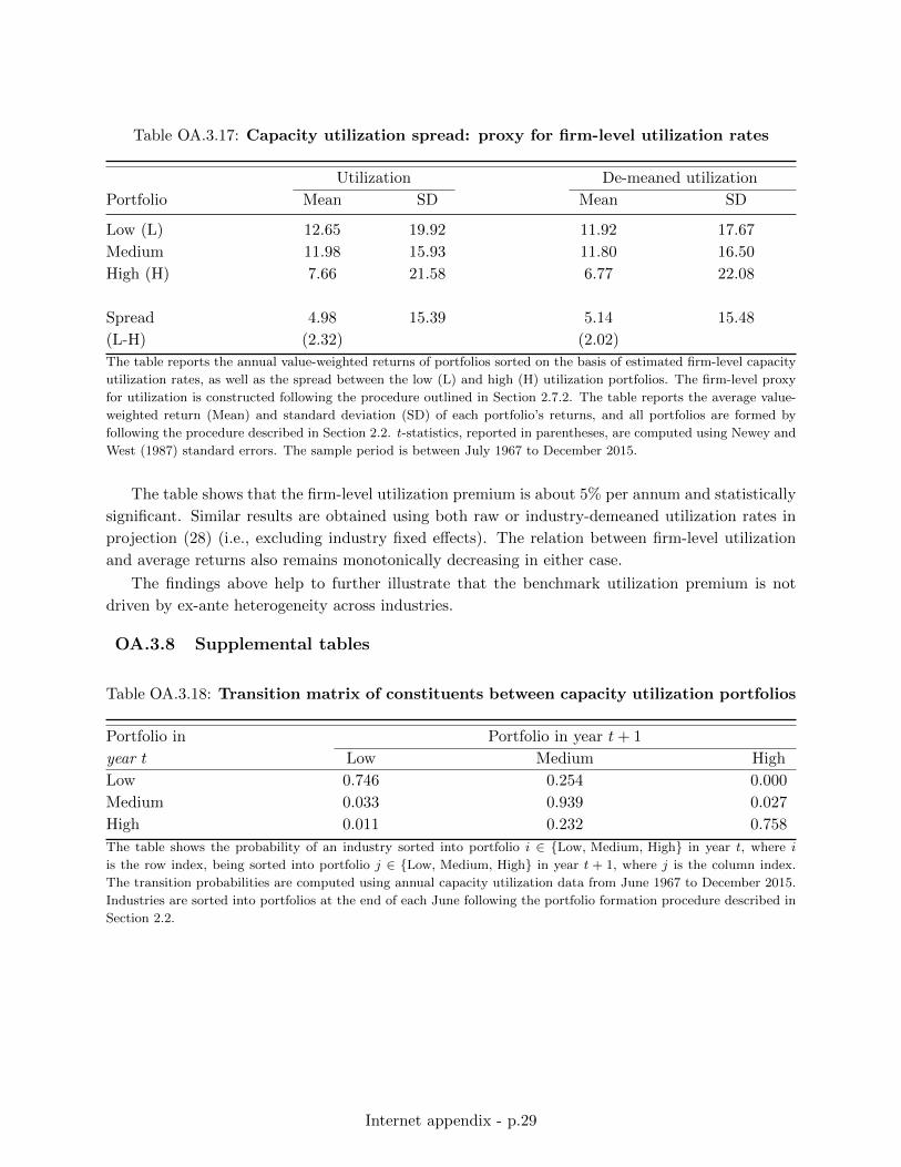
Table OA.3.17: Capacity utilization spread: proxy for firm-level utilization rates

Utilization De-meaned utilization

Portfolio Mean SD Mean SD

Low (L) 12.65 19.92 11.92 17.67

Medium 11.98 15.93 11.80 16.50

High (H) 7.66 21.58 6.77 22.08

Spread 4.98 15.39 5.14 15.48

(L-H) (2.32) (2.02)

The table reports the annual value-weighted returns of portfolios sorted on the basis of estimated firm-level capacity

utilization rates, as well as the spread between the low (L) and high (H) utilization portfolios. The firm-level proxy

for utilization is constructed following the procedure outlined in Section 2.7.2. The table reports the average value-

weighted return (Mean) and standard deviation (SD) of each portfolio’s returns, and all portfolios are formed by

following the procedure described in Section 2.2. t-statistics, reported in parentheses, are computed using Newey and

West (1987) standard errors. The sample period is between July 1967 to December 2015.

The table shows that the firm-level utilization premium is about 5% per annum and statistically

significant. Similar results are obtained using both raw or industry-demeaned utilization rates in

projection (28) (i.e., excluding industry fixed effects). The relation between firm-level utilization

and average returns also remains monotonically decreasing in either case.

The findings above help to further illustrate that the benchmark utilization premium is not

driven by ex-ante heterogeneity across industries.

OA.3.8 Supplemental tables

Table OA.3.18: Transition matrix of constituents between capacity utilization portfolios

Portfolio in Portfolio in year t+ 1

year t Low Medium High

Low 0.746 0.254 0.000

Medium 0.033 0.939 0.027

High 0.011 0.232 0.758

The table shows the probability of an industry sorted into portfolio i ∈ {Low, Medium, High} in year t, where i

is the row index, being sorted into portfolio j ∈ {Low, Medium, High} in year t + 1, where j is the column index.

The transition probabilities are computed using annual capacity utilization data from June 1967 to December 2015.

Industries are sorted into portfolios at the end of each June following the portfolio formation procedure described in

Section 2.2.

Internet appendix - p.29

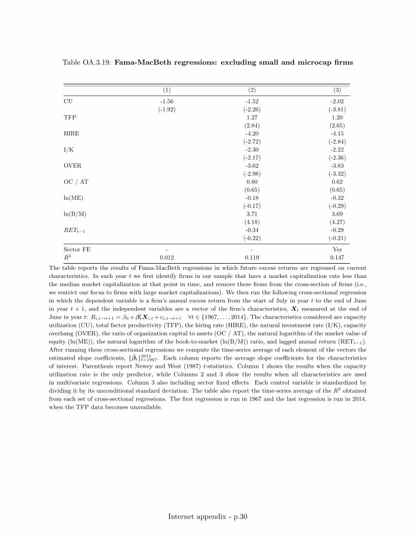
Table OA.3.19: Fama-MacBeth regressions: excluding small and microcap firms

(1) (2) (3)

CU -1.56 -1.52 -2.02

(-1.92) (-2.26) (-3.81)

TFP 1.27 1.20

(2.84) (2.65)

HIRE -4.20 -4.15

(-2.72) (-2.84)

I/K -2.30 -2.22

(-2.17) (-2.36)

OVER -3.62 -3.83

(-2.98) (-3.32)

OC / AT 0.80 0.62

(0.65) (0.65)

ln(ME) -0.18 -0.32

(-0.17) (-0.29)

ln(B/M) 3.71 3.69

(4.18) (4.27)

RETt−1 -0.34 -0.29

(-0.22) (-0.21)

Sector FE - - Yes

R2 0.012 0.119 0.147

The table reports the results of Fama-MacBeth regressions in which future excess returns are regressed on current

characteristics. In each year t we first identify firms in our sample that have a market capitalization rate less than

the median market capitalization at that point in time, and remove these firms from the cross-section of firms (i.e.,

we restrict our focus to firms with large market capitalizations). We then run the following cross-sectional regression

in which the dependent variable is a firm’s annual excess return from the start of July in year t to the end of June

in year t + 1, and the independent variables are a vector of the firm’s characteristics, Xt measured at the end of

June in year t: Ri,t→t+1 = β0 +β′tXi,t+ εi,t→t+1 ∀t ∈ {1967, . . . , 2014}. The characteristics considered are capacity

utilization (CU), total factor productivity (TFP), the hiring rate (HIRE), the natural investment rate (I/K), capacity

overhang (OVER), the ratio of organization capital to assets (OC / AT), the natural logarithm of the market value of

equity (ln(ME)), the natural logarithm of the book-to-market (ln(B/M)) ratio, and lagged annual return (RETt−1).

After running these cross-sectional regressions we compute the time-series average of each element of the vectors the

estimated slope coefficients, {βt}2014t=1967. Each column reports the average slope coefficients for the characteristics

of interest. Parenthesis report Newey and West (1987) t-statistics. Column 1 shows the results when the capacity

utilization rate is the only predictor, while Columns 2 and 3 show the results when all characteristics are used

in multivariate regressions. Column 3 also including sector fixed effects. Each control variable is standardized by

dividing it by its unconditional standard deviation. The table also report the time-series average of the R2 obtained

from each set of cross-sectional regressions. The first regression is run in 1967 and the last regression is run in 2014,

when the TFP data becomes unavailable.

Internet appendix - p.30

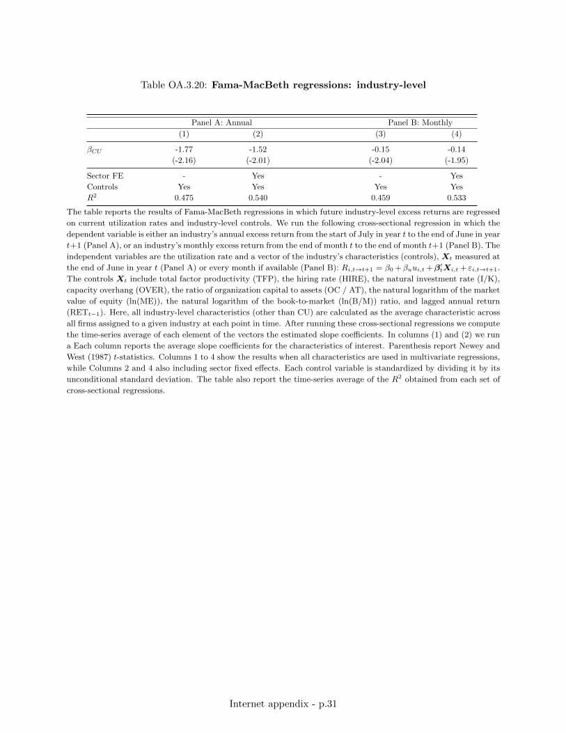
Table OA.3.20: Fama-MacBeth regressions: industry-level

Panel A: Annual Panel B: Monthly

(1) (2) (3) (4)

βCU -1.77 -1.52 -0.15 -0.14

(-2.16) (-2.01) (-2.04) (-1.95)

Sector FE - Yes - Yes

Controls Yes Yes Yes Yes

R2 0.475 0.540 0.459 0.533

The table reports the results of Fama-MacBeth regressions in which future industry-level excess returns are regressed

on current utilization rates and industry-level controls. We run the following cross-sectional regression in which the

dependent variable is either an industry’s annual excess return from the start of July in year t to the end of June in year

t+1 (Panel A), or an industry’s monthly excess return from the end of month t to the end of month t+1 (Panel B). The

independent variables are the utilization rate and a vector of the industry’s characteristics (controls), Xt measured at

the end of June in year t (Panel A) or every month if available (Panel B): Ri,t→t+1 = β0 +βuui,t +β′tXi,t + εi,t→t+1.

The controls Xt include total factor productivity (TFP), the hiring rate (HIRE), the natural investment rate (I/K),

capacity overhang (OVER), the ratio of organization capital to assets (OC / AT), the natural logarithm of the market

value of equity (ln(ME)), the natural logarithm of the book-to-market (ln(B/M)) ratio, and lagged annual return

(RETt−1). Here, all industry-level characteristics (other than CU) are calculated as the average characteristic across

all firms assigned to a given industry at each point in time. After running these cross-sectional regressions we compute

the time-series average of each element of the vectors the estimated slope coefficients. In columns (1) and (2) we run

a Each column reports the average slope coefficients for the characteristics of interest. Parenthesis report Newey and

West (1987) t-statistics. Columns 1 to 4 show the results when all characteristics are used in multivariate regressions,

while Columns 2 and 4 also including sector fixed effects. Each control variable is standardized by dividing it by its

unconditional standard deviation. The table also report the time-series average of the R2 obtained from each set of

cross-sectional regressions.

Internet appendix - p.31

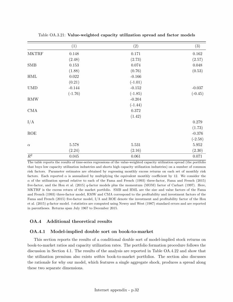
Table OA.3.21: Value-weighted capacity utilization spread and factor models

(1) (2) (3)

MKTRF 0.148 0.171 0.162

(2.48) (2.73) (2.57)

SMB 0.153 0.074 0.048

(1.88) (0.76) (0.53)

HML 0.022 -0.166

(0.21) (-1.01)

UMD -0.144 -0.152 -0.037

(-1.76) (-1.85) (-0.45)

RMW -0.204

(-1.44)

CMA 0.372

(1.42)

I/A 0.279

(1.73)

ROE -0.376

(-2.58)

α 5.578 5.531 5.952

(2.24) (2.16) (2.30)

R2 0.045 0.061 0.071

The table reports the results of time-series regressions of the value-weighted capacity utilization spread (the portfolio

that buys low capacity utilization industries and shorts high capacity utilization industries) on a number of common

risk factors. Parameter estimates are obtained by regressing monthly excess returns on each set of monthly risk

factors. Each reported α is annualized by multiplying the equivalent monthly coefficient by 12. We consider the

α of the utilization spread relative to each of the Fama and French (1993) three-factor, Fama and French (2015)

five-factor, and the Hou et al. (2015) q-factor models plus the momentum (MOM) factor of Carhart (1997). Here,

MKTRF is the excess return of the market portfolio. SMB and HML are the size and value factors of the Fama

and French (1993) three-factor model, RMW and CMA correspond to the profitability and investment factors of the

Fama and French (2015) five-factor model, I/A and ROE denote the investment and profitability factor of the Hou

et al. (2015) q-factor model. t-statistics are computed using Newey and West (1987) standard errors and are reported

in parentheses. Returns span July 1967 to December 2015.

OA.4 Additional theoretical results

OA.4.1 Model-implied double sort on book-to-market

This section reports the results of a conditional double sort of model-implied stock returns on

book-to-market ratios and capacity utilization rates. The portfolio formation procedure follows the

discussion in Section 4.1. The results of the analysis are reported in Table OA.4.22 and show that

the utilization premium also exists within book-to-market portfolios. The section also discusses

the rationale for why our model, which features a single aggregate shock, produces a spread along

these two separate dimensions.

Internet appendix - p.32

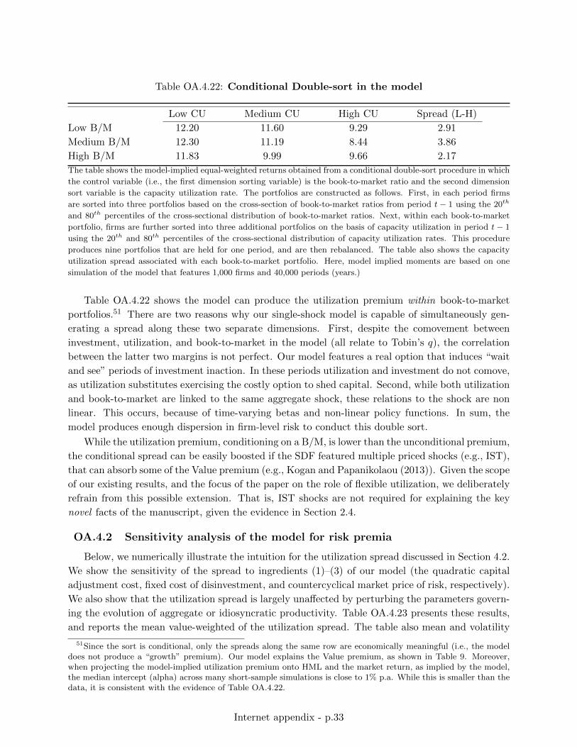
Table OA.4.22: Conditional Double-sort in the model

Low CU Medium CU High CU Spread (L-H)

Low B/M 12.20 11.60 9.29 2.91

Medium B/M 12.30 11.19 8.44 3.86

High B/M 11.83 9.99 9.66 2.17

The table shows the model-implied equal-weighted returns obtained from a conditional double-sort procedure in which

the control variable (i.e., the first dimension sorting variable) is the book-to-market ratio and the second dimension

sort variable is the capacity utilization rate. The portfolios are constructed as follows. First, in each period firms

are sorted into three portfolios based on the cross-section of book-to-market ratios from period t− 1 using the 20th

and 80th percentiles of the cross-sectional distribution of book-to-market ratios. Next, within each book-to-market

portfolio, firms are further sorted into three additional portfolios on the basis of capacity utilization in period t − 1

using the 20th and 80th percentiles of the cross-sectional distribution of capacity utilization rates. This procedure

produces nine portfolios that are held for one period, and are then rebalanced. The table also shows the capacity

utilization spread associated with each book-to-market portfolio. Here, model implied moments are based on one

simulation of the model that features 1,000 firms and 40,000 periods (years.)

Table OA.4.22 shows the model can produce the utilization premium within book-to-market

portfolios.51 There are two reasons why our single-shock model is capable of simultaneously gen-

erating a spread along these two separate dimensions. First, despite the comovement between

investment, utilization, and book-to-market in the model (all relate to Tobin’s q), the correlation

between the latter two margins is not perfect. Our model features a real option that induces “wait

and see” periods of investment inaction. In these periods utilization and investment do not comove,

as utilization substitutes exercising the costly option to shed capital. Second, while both utilization

and book-to-market are linked to the same aggregate shock, these relations to the shock are non

linear. This occurs, because of time-varying betas and non-linear policy functions. In sum, the

model produces enough dispersion in firm-level risk to conduct this double sort.

While the utilization premium, conditioning on a B/M, is lower than the unconditional premium,

the conditional spread can be easily boosted if the SDF featured multiple priced shocks (e.g., IST),

that can absorb some of the Value premium (e.g., Kogan and Papanikolaou (2013)). Given the scope

of our existing results, and the focus of the paper on the role of flexible utilization, we deliberately

refrain from this possible extension. That is, IST shocks are not required for explaining the key

novel facts of the manuscript, given the evidence in Section 2.4.

OA.4.2 Sensitivity analysis of the model for risk premia

Below, we numerically illustrate the intuition for the utilization spread discussed in Section 4.2.

We show the sensitivity of the spread to ingredients (1)–(3) of our model (the quadratic capital

adjustment cost, fixed cost of disinvestment, and countercyclical market price of risk, respectively).

We also show that the utilization spread is largely unaffected by perturbing the parameters govern-

ing the evolution of aggregate or idiosyncratic productivity. Table OA.4.23 presents these results,

and reports the mean value-weighted of the utilization spread. The table also mean and volatility

51Since the sort is conditional, only the spreads along the same row are economically meaningful (i.e., the modeldoes not produce a “growth” premium). Our model explains the Value premium, as shown in Table 9. Moreover,when projecting the model-implied utilization premium onto HML and the market return, as implied by the model,the median intercept (alpha) across many short-sample simulations is close to 1% p.a. While this is smaller than thedata, it is consistent with the evidence of Table OA.4.22.

Internet appendix - p.33

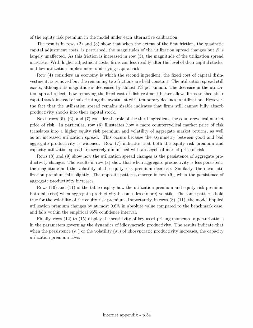
of the equity risk premium in the model under each alternative calibration.

The results in rows (2) and (3) show that when the extent of the first friction, the quadratic

capital adjustment costs, is perturbed, the magnitudes of the utilization spread changes but β is

largely unaffected. As this friction is increased in row (3), the magnitude of the utilization spread

increases. With higher adjustment costs, firms can less readily alter the level of their capital stocks,

and low utilization implies more underlying capital risk.

Row (4) considers an economy is which the second ingredient, the fixed cost of capital disin-

vestment, is removed but the remaining two frictions are held constant. The utilization spread still

exists, although its magnitude is decreased by almost 1% per annum. The decrease in the utiliza-

tion spread reflects how removing the fixed cost of disinvestment better allows firms to shed their

capital stock instead of substituting disinvestment with temporary declines in utilization. However,

the fact that the utilization spread remains sizable indicates that firms still cannot fully absorb

productivity shocks into their capital stock.

Next, rows (5), (6), and (7) consider the role of the third ingredient, the countercyclical market

price of risk. In particular, row (6) illustrates how a more countercyclical market price of risk

translates into a higher equity risk premium and volatility of aggregate market returns, as well

as an increased utilization spread. This occurs because the asymmetry between good and bad

aggregate productivity is widened. Row (7) indicates that both the equity risk premium and

capacity utilization spread are severely diminished with an acyclical market price of risk.

Rows (8) and (9) show how the utilization spread changes as the persistence of aggregate pro-

ductivity changes. The results in row (8) show that when aggregate productivity is less persistent,

the magnitude and the volatility of the equity risk premium decrease. Similarly, the mean uti-

lization premium falls slightly. The opposite patterns emerge in row (9), when the persistence of

aggregate productivity increases.

Rows (10) and (11) of the table display how the utilization premium and equity risk premium

both fall (rise) when aggregate productivity becomes less (more) volatile. The same patterns hold

true for the volatility of the equity risk premium. Importantly, in rows (8)–(11), the model implied

utilization premium changes by at most 0.6% in absolute value compared to the benchmark case,

and falls within the empirical 95% confidence interval.

Finally, rows (12) to (15) display the sensitivity of key asset-pricing moments to perturbations

in the parameters governing the dynamics of idiosyncratic productivity. The results indicate that

when the persistence (ρz) or the volatility (σz) of idiosyncratic productivity increases, the capacity

utilization premium rises.

Internet appendix - p.34

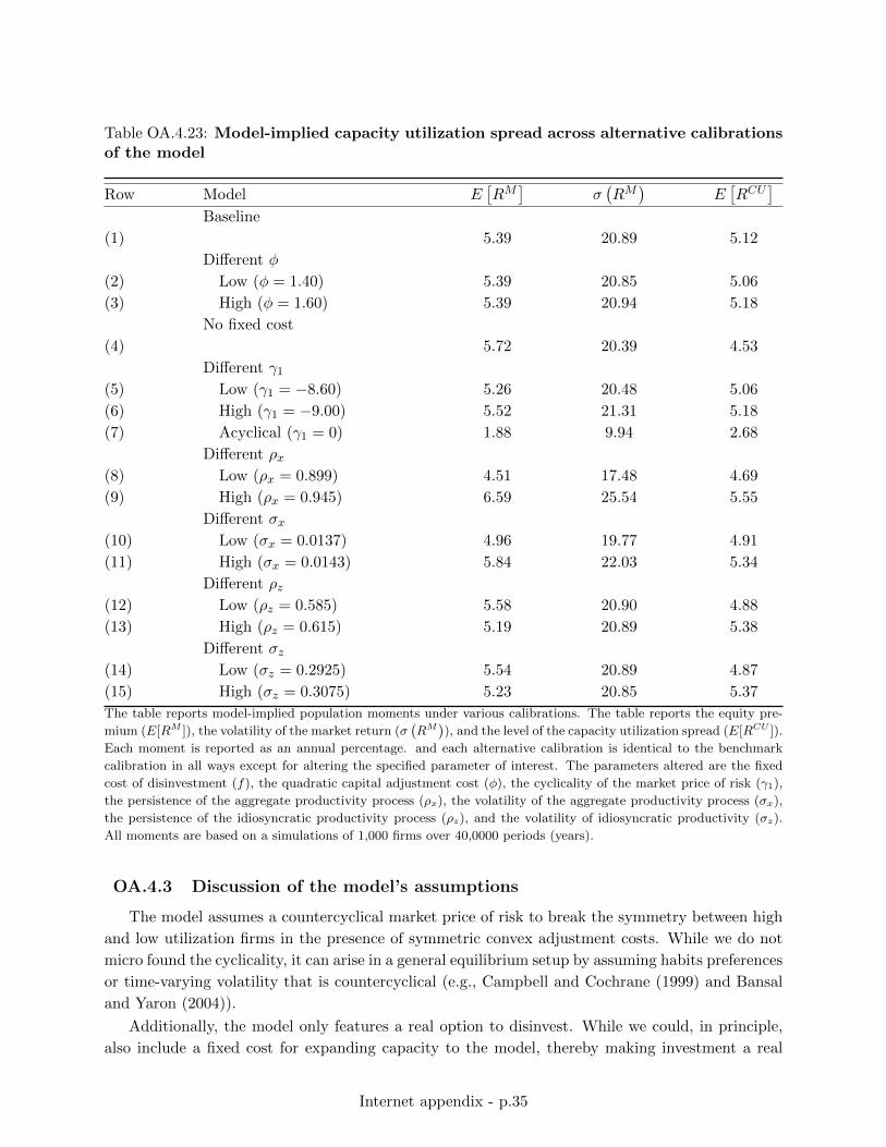
Table OA.4.23: Model-implied capacity utilization spread across alternative calibrationsof the model

Row Model E[RM

]σ(RM

)E[RCU

]Baseline

(1) 5.39 20.89 5.12

Different φ

(2) Low (φ = 1.40) 5.39 20.85 5.06

(3) High (φ = 1.60) 5.39 20.94 5.18

No fixed cost

(4) 5.72 20.39 4.53

Different γ1(5) Low (γ1 = −8.60) 5.26 20.48 5.06

(6) High (γ1 = −9.00) 5.52 21.31 5.18

(7) Acyclical (γ1 = 0) 1.88 9.94 2.68

Different ρx(8) Low (ρx = 0.899) 4.51 17.48 4.69

(9) High (ρx = 0.945) 6.59 25.54 5.55

Different σx(10) Low (σx = 0.0137) 4.96 19.77 4.91

(11) High (σx = 0.0143) 5.84 22.03 5.34

Different ρz(12) Low (ρz = 0.585) 5.58 20.90 4.88

(13) High (ρz = 0.615) 5.19 20.89 5.38

Different σz(14) Low (σz = 0.2925) 5.54 20.89 4.87

(15) High (σz = 0.3075) 5.23 20.85 5.37

The table reports model-implied population moments under various calibrations. The table reports the equity pre-

mium (E[RM ]), the volatility of the market return (σ(RM

)), and the level of the capacity utilization spread (E[RCU ]).

Each moment is reported as an annual percentage. and each alternative calibration is identical to the benchmark

calibration in all ways except for altering the specified parameter of interest. The parameters altered are the fixed

cost of disinvestment (f), the quadratic capital adjustment cost (φ), the cyclicality of the market price of risk (γ1),

the persistence of the aggregate productivity process (ρx), the volatility of the aggregate productivity process (σx),

the persistence of the idiosyncratic productivity process (ρz), and the volatility of idiosyncratic productivity (σz).

All moments are based on a simulations of 1,000 firms over 40,0000 periods (years).

OA.4.3 Discussion of the model’s assumptions

The model assumes a countercyclical market price of risk to break the symmetry between high

and low utilization firms in the presence of symmetric convex adjustment costs. While we do not

micro found the cyclicality, it can arise in a general equilibrium setup by assuming habits preferences

or time-varying volatility that is countercyclical (e.g., Campbell and Cochrane (1999) and Bansal

and Yaron (2004)).

Additionally, the model only features a real option to disinvest. While we could, in principle,

also include a fixed cost for expanding capacity to the model, thereby making investment a real

Internet appendix - p.35

option, we refrain for doing so to keep the dimensionality of the model’s parameters low. Since

the prior literature emphasizes that the adjustment costs of disinvestment are larger than those

of investment (e.g., Zhang (2005)), our model captures this notion in a parsimonious manner.

Importantly, Section 5 shows that our model with flexible utilization produces a sizable dispersion

in risk premia without relying on large adjustment frictions that distort firm-level investment

dynamics (Clementi and Palazzo, 2019).

Motivated by the empirical evidence in Sections 2.4 and OA.3.2, our framework relies on expo-

sures to a single priced state variable: productivity. Despite having only a single aggregate shock,

the model-implied CAPM alpha can be non-zero in short sample simulations (but statistically in-

distinguishable from zero when considering a 95% confidence interval), and the correlation between

utilization and investment (or book-to-market) is positive but smaller than one. The former hap-

pens because of cyclicality in risk exposures, and the latter happens as utilization can serve as a

substitute for disinvestment in downturns.

While not necessary quantitatively, featuring additional sources of aggregate risk could naturally

reduce the model-implied correlation between the utilization premium and other spreads related to

intensive-margin characteristics. We do not feature multiple shocks for parsimony.

OA.4.4 Alternative adjustment cost specification

We document that even if the capital adjustment cost function given by equation (9) is aug-

mented to include piecewise linear and quadratic terms, the model with fixed utilization is not

likely to match key investment-related moments, while generating high risk-premia spreads.

Consistent with the works of Cooper and Haltiwanger (2006), Bloom (2009), Belo and Lin

(2012), and Belo et al. (2014a), among others, we generalize the adjustment cost function employed

by our benchmark analysis to include asymmetric linear and quadratic adjustment cost. Specifically,

the adjustment cost function we employ is given by

Gi,t =

[φ+

2(nii,t)

2 1{nii,t>0} +φ−

2(nii,t)

2 1{nii,t<0} + f+1{nii,t>0} + f−1{nii,t<0}

]Ki,t. (30)

Here, ni,t ≡ Ii,tKi,t− δk denotes the net investment rate of firm i at time t, while the functions

denoted by 1{nii,t>0} (1{nii,t<0}) are indicator variables that take on a value of one when the firm

increases (reduces) its stock of capital. The adjustment parameter φ+ (φ−) capture the quadratic

adjustment cost of increasing (decreasing) capacity, while f+ (f−) captures the fixed adjustment

cost of increasing (decreasing) capacity. While our benchmark adjustment cost specification imposes

the constraints that φ+ = φ− and f+ = 0, we relax these constraints below and consider more

general specification in which φ+ 6= φ− and f+ > 0.

The model in Zhang (2005) suggests the quadratic adjustment cost for investment is around

one tenth of the magnitude of that for disinvestment. Accordingly, we focus on the case that

φ+ = φ−× 110 . Likewise, the fixed cost of investment in Belo and Lin (2012) and Belo et al. (2014a)

is approximately one third to one half of the magnitude of that for disinvestment. Consequently,

we consider the cases in which f+ = f−1 × 13 or f+ = f−1 × 1

2 . For completeness, we also consider

calibrations in which the ratios f+/f− or φ+/φ− differ from these prior studies.

Table OA.4.24 reports the model-implied time-series and cross-sectional moments of investment

rates, as well as the magnitude of cross-sectional risk premia, in a fixed-utilization model featuring

asymmetric capital adjustment costs. Rows (2) to (6) of the table consider calibrations in which

Internet appendix - p.36

φ+ = φ− in equation (30), identical to our baseline calibration reported in row (1), but f+ > 0.

We keep in f− at a positive value, consistent with the reason outlined in Section 3.1. By and large,

perturbing introducing an upside linear adjustment cost does not help to reconcile the data. For

instance, when f+ = f− × 12 in row (6) the dispersion and volatility of investment rates, as well as

the magnitudes of the risk premia, remain far lower than their counterparts in the data.

Rows (7) to (9) of the table keep f+ = 0 (identical to our baseline model) but allow for

asymmetry in the quadratic adjustment costs (i.e., φ+ 6= φ−). Focusing on row (8), a calibration

in which φ+ = φ− × 110 , shows that this asymmetry can reconcile cross-sectional moments of

investment rates with the data (e.g., the cross-sectional skewness is about 1.8 in both the model

and the data). However, the same calibration fails to match the time-series moments of investment

rates and risk premia. Specifically, the model-implied time-series volatility (skewness) of investment

rates is almost twice (five times) as high as its empirical counterpart. Moreover, risk premia in this

model are too low compared to the data.

In rows (10) and (11) the adjustment cost function is calibrated to feature both asymmetric

linear and quadratic adjustment costs. Here, the degree of asymmetry follows the degrees of

asymmetry considered in the literature (see, e.g., Zhang (2005), Belo and Lin (2012), and Belo

et al. (2014a)). The results indicate that even with the most general form of the asymmetric

adjustment costs, the fixed-utilization model is only able to reconcile the cross-sectional moments

at the expense of not matching the time-series of investment and risk premia. For instance, row

(10) is quite similar to row (8) in terms of matches and mismatches.

To complement the above evidence, we also search for a value of φ− that is able to match

the value premium, similarly to the exercise presented in Section 5.3. The search result yields

two conclusions, which are almost identical to Section 5.3. First, even though we feature a more

elaborate adjustment cost, as in Cooper and Haltiwanger (2006), we still need to increase the

exogenous amount of capital friction compared to the flexible utilization model. We find that the

downside quadratic adjustment cost φ− has to be doubled. That is, a calibration in which φ− = 3,

φ+ = φ−/10 and f+ = f−/3 yields a value premium of 3.5%, which is close to the data. Second, this

higher value of φ− renders two prominent counterfactual moments for investment: the time-series

skewness of investment is much larger than the data (about 3.5), and the cross-sectional dispersion

is about a half of the data (about 0.08).

To conclude, the evidence points out that asymmetry in the linear cost has only a marginal

effect on the results, while asymmetry in φ helps only for the cross-section of investment. In

particular, row (8) shows that without deviating from standard values of α, δk, or αl, the fixed

utilization real option model cannot match the data. Importantly, even if such calibration was

found, flexible utilization would still offer valuable merit: it provides a way to rely on a lower

dimensional adjustment cost function, and endogonize the implications of additional exogenous

calibration parameters, using a micro-founded margin. The only additional model parameter needed

to accommodate flexible utilization is λ.

Internet appendix - p.37

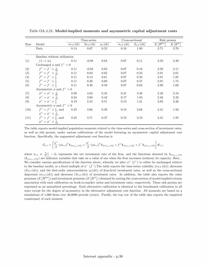
Table OA.4.24: Model-implied moments and asymmetric capital adjustment costs

Time-series Cross-sectional Risk premia

Row Model σTS (ik) STS (ik) ρ1 (ik) σCS (ik) SCS (ik) E[Rbm

]E[Rik

]Data 0.14 0.67 0.52 0.16 1.89 3.71 3.70

Baseline without utilization

(1) (λ→∞) 0.11 -0.09 0.64 0.07 0.11 2.93 2.30

Unchanged φ and f+ > 0

(2) f+ = f− × 120

0.11 -0.03 0.63 0.07 0.16 2.92 2.11

(3) f+ = f− × 110

0.11 0.03 0.62 0.07 0.23 2.91 2.01

(4) f+ = f− × 15

0.11 0.13 0.61 0.07 0.33 2.91 1.85

(5) f+ = f− × 13

0.11 0.26 0.60 0.07 0.47 2.91 1.74

(6) f+ = f− × 12

0.11 0.40 0.59 0.07 0.63 2.90 1.60

Asymmetric φ and f+ = 0

(7) φ+ = φ− × 120

0.30 4.83 0.34 0.21 2.56 2.28 2.18

(8) φ+ = φ− × 110

0.24 3.60 0.42 0.17 1.83 2.46 2.22

(9) φ+ = φ− × 15

0.19 2.45 0.51 0.13 1.21 2.62 2.26

Asymmetric φ and f+ > 0

(10) f+ = f− × 13, and 0.25 3.66 0.39 0.18 2.08 2.41 1.92

φ+ = φ− × 110

(11) f+ = f− × 12, and 0.25 3.71 0.37 0.18 2.19 2.41 1.85

φ+ = φ− × 110

The table reports model-implied population moments related to the time-series and cross-section of investment rates,

as well as risk premia, under various calibrations of the model featuring an asymmetric capital adjustment cost

function. Specifically, the augmented adjustment cost function is

Gi,t =

[φ+

2(nii,t)

2 1{nii,t>0} +φ−

2(nii,t)

2 1{nii,t<0} + f+1{nii,t>0} + f−1{nii,t<0}

]Ki,t,

where ni,t ≡ Ii,tKi,t

− δk represents the net investment rate of the firm, and the functions denoted by 1{nii,t>0}

(1{nii,t<0}) are indicator variables that take on a value of one when the firm increases (reduces) its capacity. Here, .

We consider various specifications of the function above, whereby we alter φ+ (f+) to either be unchanged relative

to the baseline model, or a fixed multiple of φ− (f−).The table reports the time-series volatility (σTS (ik)), skewness

(STS (ik)), and the first-order autocorrelation (ρ (ik)) of firm-level investment rates, as well as the cross-sectional

dispersion (σCS (ik)) and skewness (SCS (ik)) of investment rates. In addition, the table also reports the value

premium (E[Rbm

]) and investment premium (E

[Rik

]) obtained by sorting the cross-section of model-implied returns

association with each calibration on book-to-market ratios and investment rates, respectively. These risk premia are

expressed as an annualized percentage. Each alternative calibration is identical to the benchmark calibration in all

ways except for the degree of asymmetry in the alternative adjustment cost function. All moments are based on a

simulations of 1,000 firms over 40,0000 periods (years). Finally, the top row of the table also reports the empirical

counterpart of each moment.

Internet appendix - p.38

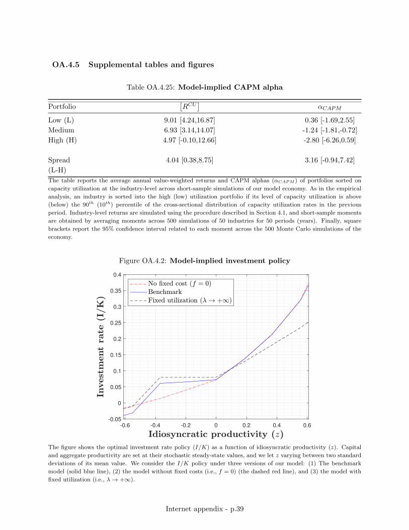
OA.4.5 Supplemental tables and figures

Table OA.4.25: Model-implied CAPM alpha

Portfolio[RCU

]αCAPM

Low (L) 9.01 [4.24,16.87] 0.36 [-1.69,2.55]

Medium 6.93 [3.14,14.07] -1.24 [-1.81,-0.72]

High (H) 4.97 [-0.10,12.66] -2.80 [-6.26,0.59]

Spread 4.04 [0.38,8.75] 3.16 [-0.94,7.42]

(L-H)

The table reports the average annual value-weighted returns and CAPM alphas (αCAPM ) of portfolios sorted on

capacity utilization at the industry-level across short-sample simulations of our model economy. As in the empirical

analysis, an industry is sorted into the high (low) utilization portfolio if its level of capacity utilization is above

(below) the 90th (10th) percentile of the cross-sectional distribution of capacity utilization rates in the previous

period. Industry-level returns are simulated using the procedure described in Section 4.1, and short-sample moments

are obtained by averaging moments across 500 simulations of 50 industries for 50 periods (years). Finally, square

brackets report the 95% confidence interval related to each moment across the 500 Monte Carlo simulations of the

economy.

Figure OA.4.2: Model-implied investment policy

-0.6 -0.4 -0.2 0 0.2 0.4 0.6

-0.05

0

0.05

0.1

0.15

0.2

0.25

0.3

0.35

0.4

The figure shows the optimal investment rate policy (I/K) as a function of idiosyncratic productivity (z). Capital

and aggregate productivity are set at their stochastic steady-state values, and we let z varying between two standard

deviations of its mean value. We consider the I/K policy under three versions of our model: (1) The benchmark

model (solid blue line), (2) the model without fixed costs (i.e., f = 0) (the dashed red line), and (3) the model with

fixed utilization (i.e., λ→ +∞).

Internet appendix - p.39

OA.5 Utilization and depreciation: Empirical evidence and model extensions

OA.5.1 Utilization and depreciation dynamics

Equation (8) suggests that firms’ depreciation rates should correlate positively with their uti-

lization rates. In this section we check this prediction and explore its implications for the accuracy

and the frequency of depreciation’s measurement.

We examine the relation between utilization and depreciation via the projection

∆δj,t = dj + du∆uj,t + dxXj,t + εj,t,

where j denotes an industry index, ∆δj,t is the log growth of industry j’s depreciation rate from

BEA, ∆uj,t is the log growth of industry j’s utilization rate, and Xj,t is a control variable. We

use the log growth of depreciation and utilization to reduce persistence in these variables, and

to account for a non-linear relation between the level of the two. All variables are standardized

for the ease of interpretation. The results of the projection are reported in Table OA.5.26. In

columns (1) and (2) of the table we run the projection without any controls. We show that the

simple correlation between log depreciation growth and log utilization growth is 30%, and that this

correlation is not affected by the inclusion of industry fixed effects.

Table OA.5.26: Empirical relation between capacity utilization and depreciation rates

(1) (2) (3) (4) (5) (6)

βUTIL 0.30 0.30 0.28 0.28

(3.11) (3.14) (2.80) (2.83)

βCOMP 0.03 0.03 0.13 0.14

(3.50) (3.53) (3.54) (3.58)

Industry FE No Yes No Yes No Yes

R2 0.09 0.09 0.02 0.02 0.10 0.10

The table reports the empirical relation between the industry-level capacity utilization rate, industry-level depre-

ciation rate from the BEA, and industry-level depreciation rate from Compustat. In each specification considered

in the table we run projections of the log-growth rate of BEA-implied depreciation on the log-growth rates of ca-

pacity utilization and Compustat-implied depreciation rates, and standardize all variables for ease of interpretation.

Columns (1), (3), and (5) of the table estimated pooled-OLS regressions, whereas columns (2), (4), and (6) of the

table estimate panel regressions including industry fixed effects. t-statistics, reported in parentheses, and computed

using standard errors clustered at the industry level. Finally, the time span underlying the regressions is from January

1967 to December 2015.

Recent studies in production-based asset pricing show that BEA- and Compustat-implied de-

preciation rates are strikingly different. The use of one over the other can lead to economically

sizable differences in the distribution of gross investment rates (e.g., Clementi and Palazzo (2019);

Bai et al. (2019)). In line with these papers, columns (3) and (4) of Table OA.5.26 demonstrate the

discrepancy between these two depreciation measures. We set Xj,t to be the log growth of industry

j’s Compustat-based depreciation rate, and restrict du to zero. The correlation between the growth

of these depreciation measures is only 3%.52

In columns (5) and (6) we do not restrict du to be zero. First, the positive correlation between

BEA-implied depreciation growth and utilization growth remains positive and sizable when con-

trolling for Compustat-implied depreciation. Second, the (partial) correlation between the growth

52We describe the measurement of the these depreciation rates in Section OA.1 of the Online Appendix.

Internet appendix - p.40

rates of BEA- and Compustat-implied depreciation increases to 14%. Thus, utilization narrows

the wedge between these two measures. While measurement error may exist in both measures, the

fact that the correlation between the two increases when controlling for utilization suggests that

utilization can be used to accurately filter the true depreciation rate. We briefly illustrate this

point in the next subsection.

OA.5.2 High-frequency depreciation based on utilization data

As utilization data is available at the monthly frequency, the utilization-implied depreciation

rate we propose is computed at a higher frequency than depreciation rates implied by either BEA

or Compustat. First, to be consistent with the model, we adjust each industry’s utilization rate

to have a mean of one. Then, for each industry j, we obtain a utilization-implied depreciation

rate, δ(uj), by applying equation (8) to the industry’s utilization data. Here, we use the model

parameters in Table 8. Second, we average these depreciation rates across all industries to obtain an

aggregate utilization-implied depreciation rate, δ(uagg). Third, we adjust δ(uagg) to share the same

trend as the aggregate depreciation rate from the BEA. We do this by combining the business-cycle

component of δ(uagg) with the stochastic trend component of the BEA’s aggregate depreciation

rate.53 We obtain the components of each time-series using the Hodrick and Prescott (1997) filter.

In Figure OA.5.3 we plot the monthly time-series of δ(uagg) alongside the trend of the BEA’s

aggregate depreciation rate. By construction, the two time-series share the same trend, but δ(uagg)

shows high-frequency business-cycle fluctuations around this common trend. These fluctuations

could be important as they amplify the volatility of gross investment rates and can help to reconcile

the dynamics of BEA- and Compustat-implied depreciation rates.

OA.5.3 The effect of stochastic depreciation shocks

We pursue an extension of our model motivated by the empirical evidence in Section OA.5.1.

Specifically, while our baseline model assumes that depreciation rates correlate positively with uti-

lization rates (recall equation (8)), Table OA.5.26 shows that these two quantities comove together,

but not perfectly. As a result, we modify equation (8) to also feature an exogenous shock to the

depreciation rate. This implies that a firm’s depreciation rate becomes a combination of (i) its

choice of utilization rate, and (ii) a stochastic shock. This augmented depreciation function is

δ(ui,t) = δk + δu

[u1+λi,t − 1

1 + λ

]+ dt, where dt+1 = ρddt + σdε

δt+1, (31)

and εδt is a standard normal i.i.d. shock to depreciation. Since depreciation shocks can be corre-

lated with aggregate productivity, we consider two extreme cases: shocks that are both perfectly

positively and perfectly negatively correlated with aggregate productivity.

We calibrate ρd and σd such that the largest value of |dt| in a discrete state space with a

truncated support (i.e., two standard deviations from zero) causes the depreciation rate to change

by up to 2.58%. As the unconditional depreciation rate in the model (δk) is 8%, the impact of the

largest depreciation shock causes a firm’s depreciation rate to change by roughly 33% compared

to its unconditional mean. Given the large magnitude of these calibrated depreciation shocks, this

exercises places an upper bound on the effect that these shocks can have on the utilization premium.

53The third step is optional and meant to ensure both series follow the same trend. An alternative measure of theutilization-implied depreciation rate involves only the first two steps, with similar results.

Internet appendix - p.41

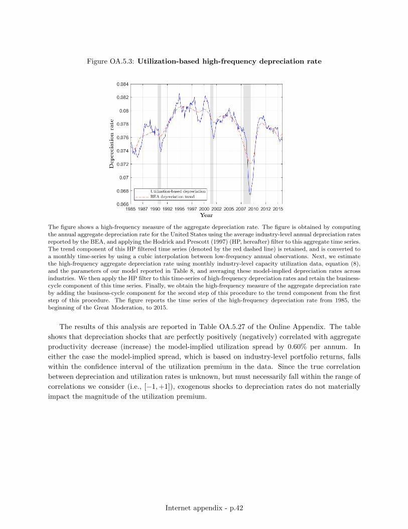
Figure OA.5.3: Utilization-based high-frequency depreciation rate

The figure shows a high-frequency measure of the aggregate depreciation rate. The figure is obtained by computingthe annual aggregate depreciation rate for the United States using the average industry-level annual depreciation ratesreported by the BEA, and applying the Hodrick and Prescott (1997) (HP, hereafter) filter to this aggregate time series.The trend component of this HP filtered time series (denoted by the red dashed line) is retained, and is converted toa monthly time-series by using a cubic interpolation between low-frequency annual observations. Next, we estimatethe high-frequency aggregate depreciation rate using monthly industry-level capacity utilization data, equation (8),and the parameters of our model reported in Table 8, and averaging these model-implied depreciation rates acrossindustries. We then apply the HP filter to this time-series of high-frequency depreciation rates and retain the business-cycle component of this time series. Finally, we obtain the high-frequency measure of the aggregate depreciation rateby adding the business-cycle component for the second step of this procedure to the trend component from the firststep of this procedure. The figure reports the time series of the high-frequency depreciation rate from 1985, thebeginning of the Great Moderation, to 2015.

The results of this analysis are reported in Table OA.5.27 of the Online Appendix. The table

shows that depreciation shocks that are perfectly positively (negatively) correlated with aggregate

productivity decrease (increase) the model-implied utilization spread by 0.60% per annum. In

either the case the model-implied spread, which is based on industry-level portfolio returns, falls

within the confidence interval of the utilization premium in the data. Since the true correlation

between depreciation and utilization rates is unknown, but must necessarily fall within the range of

correlations we consider (i.e., [−1,+1]), exogenous shocks to depreciation rates do not materially

impact the magnitude of the utilization premium.

Internet appendix - p.42

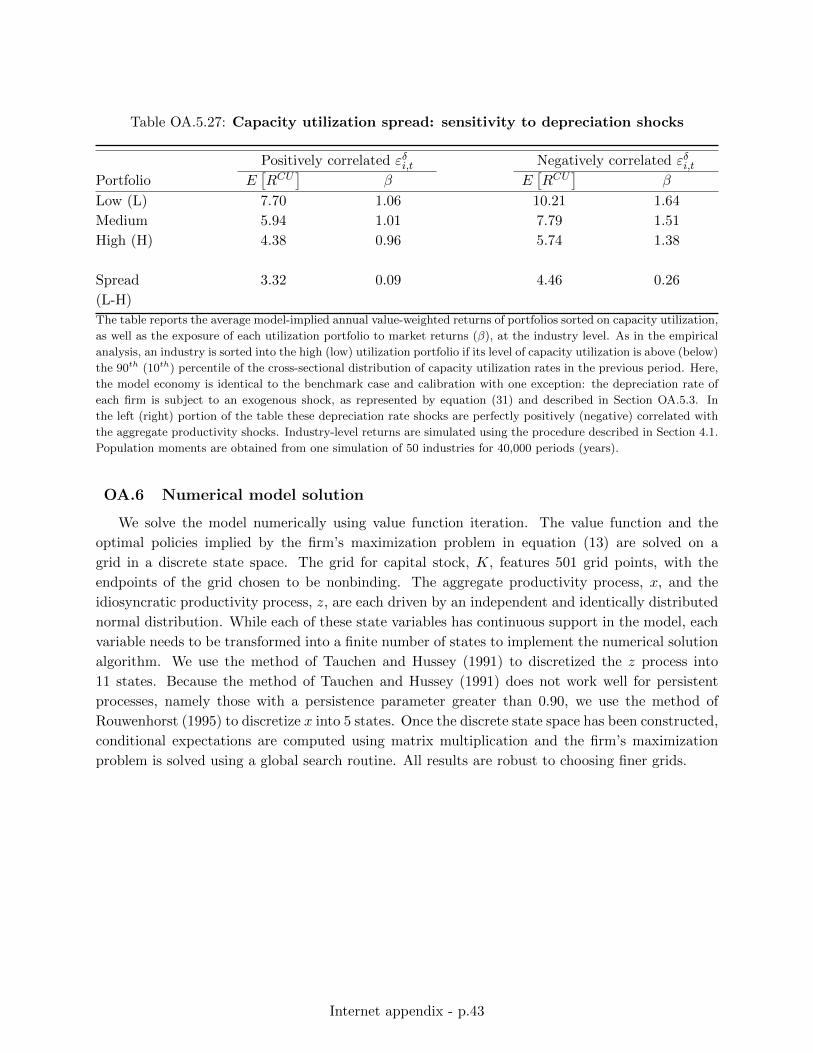
Table OA.5.27: Capacity utilization spread: sensitivity to depreciation shocks

Positively correlated εδi,t Negatively correlated εδi,tPortfolio E

[RCU

]β E

[RCU

]β

Low (L) 7.70 1.06 10.21 1.64

Medium 5.94 1.01 7.79 1.51

High (H) 4.38 0.96 5.74 1.38

Spread 3.32 0.09 4.46 0.26

(L-H)

The table reports the average model-implied annual value-weighted returns of portfolios sorted on capacity utilization,

as well as the exposure of each utilization portfolio to market returns (β), at the industry level. As in the empirical

analysis, an industry is sorted into the high (low) utilization portfolio if its level of capacity utilization is above (below)

the 90th (10th) percentile of the cross-sectional distribution of capacity utilization rates in the previous period. Here,

the model economy is identical to the benchmark case and calibration with one exception: the depreciation rate of

each firm is subject to an exogenous shock, as represented by equation (31) and described in Section OA.5.3. In

the left (right) portion of the table these depreciation rate shocks are perfectly positively (negative) correlated with

the aggregate productivity shocks. Industry-level returns are simulated using the procedure described in Section 4.1.

Population moments are obtained from one simulation of 50 industries for 40,000 periods (years).

OA.6 Numerical model solution

We solve the model numerically using value function iteration. The value function and the

optimal policies implied by the firm’s maximization problem in equation (13) are solved on a

grid in a discrete state space. The grid for capital stock, K, features 501 grid points, with the

endpoints of the grid chosen to be nonbinding. The aggregate productivity process, x, and the

idiosyncratic productivity process, z, are each driven by an independent and identically distributed

normal distribution. While each of these state variables has continuous support in the model, each

variable needs to be transformed into a finite number of states to implement the numerical solution

algorithm. We use the method of Tauchen and Hussey (1991) to discretized the z process into

11 states. Because the method of Tauchen and Hussey (1991) does not work well for persistent

processes, namely those with a persistence parameter greater than 0.90, we use the method of

Rouwenhorst (1995) to discretize x into 5 states. Once the discrete state space has been constructed,

conditional expectations are computed using matrix multiplication and the firm’s maximization

problem is solved using a global search routine. All results are robust to choosing finer grids.

Internet appendix - p.43