The utilisation of an adaptive 3D Gauss-Legendre quadrature in the simulation of sound propagation outdoors for sources with variable power distribution

Technical note

The utilisation of an adaptive 3DGauss-Legendre quadrature in the simulationof sound propagation outdoors for sources

with variable power distribution

Shahrir Abdullah *, Mohd. Jailani Mohd. Nor

Department of Mechanical and Materials Engineering, Faculty of Engineering, Universiti Kebangsaan

Malaysia, 43600 UKM Bangi, Selangor, Malaysia

Received 28 September 1999; received in revised form 7 January 2000; accepted 13 March 2000

Abstract

This paper presents the utilisation of sound propagation outdoors using an adaptive 3DGauss-Legendre quadrature method for generating contours for sound pressure levels, which

is based on the di�used-®eld theory. The main advantage of this method is that it takes intoaccount the geometry of the de®ned sound sources and produces the appropriate contoursconforming to the shape of the sources. In addition, the variation in sound power distribution

can also be simulated, where the appropriate distribution is decided from measurements. Bymodelling any source shape as an array of point sources which are in forms of lines, planes or3D blocks, sound level at any position can be calculated using line, surface and volume inte-grals, respectively. This model is mostly suitable to be used for modelling huge sound sources

such as power plants, or highways, and has been successfully used in the EnvironmentalImpact Assessment studies involving noise issues. # 2000 Elsevier Science Ltd. All rightsreserved.

Keywords: Sound propagation outdoors; Noise simulation; Pressure level contours; Adaptive Gauss

quadrature; 3D numerical integration

1. Introduction

Sound propagation outdoors is commonly discussed in three components: source,path and receiver [1]. First, the source emits sound power, resulting in sound levels

Applied Acoustics 62 (2001) 65±83

www.elsevier.com/locate/apacoust

0003-682X/01/$ - see front matter # 2000 Elsevier Science Ltd. All rights reserved.

PI I : S0003-682X(00 )00021 -9

* Corresponding author. Fax: +603-8259659.

E-mail address: [email protected] (S. Abdullah).

that can be measured in the vicinity of the source. Next, the sound level diminishesas the sound propagates outward along the path from the source to receiver. Finally,sound levels from all sources combine at the receiver.Early investigations for sound propagation outdoors are already in the literature,

for example in [2±4]. From these references, the equations used to calculate soundlevel were a mixture of experimental and physical scale models, guided by theory.O�cial methods were also being established as reported in [1,5±7], where thesemethods can provide guidance in performing noise assessment analysis. By usingthese guidelines, outdoor noise propagation at a site can be studied. In many cases,however, only the pressure levels for the point source were determined analytically,whereas others were determined empirically.Up to this date, there are a number of computer schemes, which had been

designed for this purpose [6,9±12], and the accuracy of �2-5 dB had been claimed[8,13,14]. However, these schemes also generally rely heavily upon empirical infor-mation determined from ®eld survey, but gradually empiricism is being replacedwith well-established analysis based upon extensive research. All of these methodsare known as di�use-®eld theory, which is based on the spherical divergence of pointsource and can be extended to other shapes as an array of point sources. Other morecomprehensive prediction models include the method of images [15,16], whichreplaces re¯ected sound rays with a direct ray, and the ray tracing technique [17,18],which generates a large number of rays from sources to be followed as they propa-gate in the ®eld. However, both of the methods are more suitable for indoor noisepropagation where reverberation is signi®cant.Analytical solution for a ®nite and in®nite line source had been derived by Rathe

[19]. Although this formulation has been originally derived for a straight line, it canbe adapted to model complex and curvy line sources by segmenting it into a groupof piecewise lines. For plane sources, its analytical solution has been developed byHohenwarter [20], and thus buildings with interior sources, such as power stationsand boiler houses, can be modelled as a group of plane radiators. However,Hohenwarter's formulation utilised the integration of a solid angle for a particularsource plane, which is equal to zero at any position inline with the plane, and thisleads to logarithmic singularity at those particular positions.Therefore, this paper presents an alternative method to calculate pressure levels

for the given sound sources, and the main focus is to obtain pressure level contoursin a large site, which conform to the shapes of the source. In reality, the sourcegeometry and its power distribution can be very complex, such as curvy highways orrailway interchanges to be modelled as curvy line sources, process plant equipmentand power station building should be treated as an array of 3D prism blocks withvariable power distribution. The proposed method will integrate the analyticalsolution of the point spherical source via line, surface and volume integrals, respec-tively. The integration was carried out numerically via an adaptive 3D Gauss-Legendre quadrature method to allow sound power be de®ned in terms of its den-sity, where this scheme enables the variation of source power level throughout thegeometry. This variable power density can be seen as an integrated feature of sourcedirectivity.

66 S. Abdullah, M.J.M. Nor /Applied Acoustics 62 (2001) 65±83

2. Theoretical background

The following sections give brief explanations on the theory of sound propagationoutdoors.

2.1. Di�use-®eld theory

Generally, the di�use-®eld theory is based on the spherical divergence of a pointsource in a free space. The sound pressure p due to a point source of power Wdecreases with the distance r between the source and the receiver. Since a soundwave is generated through collision among air molecules, its pressure is usuallymeasured and analysed in terms of its time-averaged squared, or also known as theroot-mean-square, pressure prms, its relation with the sound power W is [7]

p2rms ��cQW

4�r2�1�

where �, c and Q are density of air, speed of sound in air and source directivity in thereceiver direction, respectively. Based on Eq. (1), the formulation for noise level canbe established in logarithmic form, such that

Lp � LW � 10 log10Q

4�r2

� �� 10 log10

�cWref

p2ref

� ��2�

Lp � LW � 10 log10 Qÿ 20 log10 rÿ C �3�

Here, the referenced values for the sound power and pressure are Wref � 10ÿ2 Wand pref � 2� 10ÿ5 Pa, respectively. In Eq. (3), and the second left-hand side term10 log10 Q is also known as directivity index (DI), while the last left-hand term Crepresents the default attenuation where its formula can be extracted from Eq. (2).Eq. (3) results in the reduction of 6 dB for a doubling distance and can be used tomodel small sound sources radiating spherical waves, such as pumps and processequipment, or even a building from a certain distance.

2.2. Formulation for sound propagation outdoors

The basic equation of sound propagation outdoors explicitly contains sourcedirectivity, the e�ects of wave divergence and excess attenuation from all signi®cantpropagation mechanisms between source and receiver. Generally for a source withsound power level LW, the equation for the sound pressure level Lp is [7]

Lp � LW �DIÿ Adiv ÿ Aexc ÿ C �4�

In this work, for shaped sources, the term DI is omitted and the source directivityis determined by the power density distribution de®ned for each shaped source.

S. Abdullah, M.J.M. Nor /Applied Acoustics 62 (2001) 65±83 67

Also, Adiv is the attenuation due to wave divergence and Aexc is the excess attenua-tion due to other factors such as barrier, ground re¯ection or absorption, airabsorption, foliage, terrain pro®le and meteorological e�ects, and C is the defaultattenuation as discussed earlier. For a point source, the wave divergence attenuationAdiv is represented by the term 20 log10 r in Eq. (3). At present, the most successfulschemes utilise a mixture of both theory and empiricism as discussed in [7].

2.3. Analytical solution for shaped sources

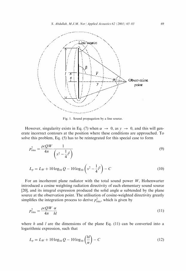
For a straight incoherent line source having a ®nite length l and a sound powerdistribution w x� �, as illustrated in Fig. 1, it is equivalent to having a group of pointsources aligned in a line and the root-mean-square pressure prms can be derived usingEq. (1), that is [15]

p2rms ��x2x1

�cQ

4��w x� �r2

dx �5�

where x is the curvilinear coordinate along the line source and r is the variable dis-tance between the real position of x and the observation point. If the parameters �,c, Q and w x� � are all constants, and w x� � �W=l, where W is the total sound powerfor the source, and if the line is straight, the integration of Eq. (5) leads to [15]

p2rms ��cQW

4�y��l

�6�

where y � r� sin � is the normal distance from the source to the observation point, r� isthe mean distance between the centre of the source and the observation point and �is the angle subtended by the source at the observation point (see Fig. 1). This Eq.(6) can be expressed in logarithmic form such that

Lp � LW � 10 log10 Qÿ 10 log10 ly=�� ÿ C �7�

In a far ®eld (r�� l), it can be shown that Eq. (7) reduces to a form similar to Eq.(3) and, from this distance, the line source can be treated as a point source.This formulation may be used to model line sources, which radiate cylindrical

waves (for in®nite length), or elliptic waves (for ®nite length), such as tra�c andrailways. For a considerably long, steady-state noise source, it may be more con-venient to express the source power in form of power per unit length w �W=l. Inthe case where w is constant, for a straight in®nite source length l ! 1; � ! �� ,Eq. (5) reduces to

Lp � Lw � 10 log10 Qÿ 10 log10 y=�� ÿ C �8�

which also results in the reduction of 3 dB for a doubling distance.


However, singularity exists in Eq. (7) when � ! 0, as y ! 0, and this will gen-erate incorrect contours at the position where these conditions are approached. Tosolve this problem, Eq. (5) has to be reintegrated for this special case to form

p2rms ��cQW

4�� 1

x2 ÿ 1

4l2

� � �9�

Lp � LW � 10 log10 Qÿ 10 log10 x2 ÿ 1

4l2

� �ÿ C �10�

For an incoherent plane radiator with the total sound power W, Hohenwarterintroduced a cosine weighting radiation directivity of each elementary sound source[20], and its integral expression produced the solid angle � subtended by the planesource at the observation point. The utilisation of cosine-weighted directivity greatlysimpli®es the integration process to derive p2rms, which is given by

p2rms ��cQW

4��hl

�11�

where h and l are the dimensions of the plane Eq. (11) can be converted into alogarithmic expression, such that

Lp � LW � 10 log10 Qÿ 10 log10hl

�

� �ÿ C �12�

Fig. 1. Sound propagation by a line source.


This formulation may be used to model sound sources, which radiate planarwaves conforming to the source geometry such building walls with interior sourcelike power stations and boiler houses. However, the use of this formulation can leadserious singularity problem at any position in-plane with the radiator since � ! 0(see Eq. 12).

2.4. Excess attenuation

During the calculation process, the formulation for air attenuation is adaptedfrom Sutherland et al. [21], who has presented a table of air absorption coe�cientsper 1000 m travelling distance for each octave band, and the coe�cients are depen-dent on the ambient temperature and humidity of the studied site. The formulationfor ground attenuation for each octave band is presented in [6], which is dependenton ground absorption parameter G, that is, G equals to zero for acoustically hardground and unity for acoustically soft ground. Other types of attenuation which aredue to barrier, foliage and terrain pro®les, are excluded in this study since its e�ectare more localised and it require more extensive data such as the exact position andextension of the barrier or foliage, and earth surface topology for the particular site.Hence, this study applies to a huge area in which these factors are not signi®cant.Furthermore, attenuation due to the meteorological aspects such as winds is alsoexcluded since these e�ects are transient, whereas the study will focus on the generalsteady-state propagation of sound waves.

3. Modelling formulation

The following sections discuss the mathematical and numerical formulations,which are utilised in this study.

3.1. Integral equations

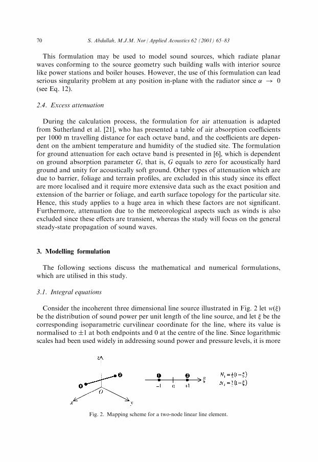
Consider the incoherent three dimensional line source illustrated in Fig. 2 let w �� be the distribution of sound power per unit length of the line source, and let � be thecorresponding isoparametric curvilinear coordinate for the line, where its value isnormalised to �1 at both endpoints and 0 at the centre of the line. Since logarithmicscales had been used widely in addressing sound power and pressure levels, it is more

Fig. 2. Mapping scheme for a two-node linear line element.


convenient to express w in the form of its distributed sound power Lw. From Fig. 3,the relation between the Cartesian coordinates, their derivatives and the distributedpower level with the parameter � can be written as

x �Xni�1

Ni �� xi; y �Xni�1

Ni �� yi; z �Xni�1

Ni �� zi; Lw �Xni�1

Ni �� Lwi

@x

@��Xni�1

@Ni

@��xi; @y

@��Xni�1

@Ni

@��yi; @z

@��Xni�1

@Ni

@��zi �13�

where n is the number of points which de®nes the line element, and in this casen � 2. Also, Ni is the shape, or interpolation function of the element (see Fig. 2), andits implementation is similar to that employed in the well-known ®nite elementanalysis [22].If �, c andQ are all constants, thus Eq. (5) can be rewritten in form of line integral as

p2rms ��cQ

4�

��1ÿ1

wd�

xÿ xr� �2� yÿ yr� �2� zÿ zr� �2 �@x

@�i� @y

@�j� @z

@�k

�14�

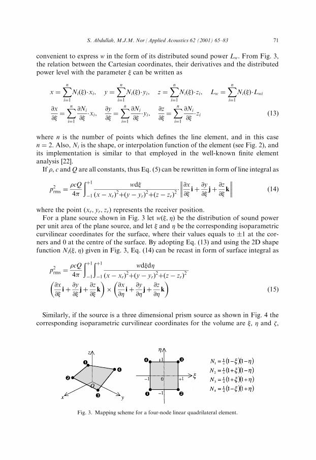
where the point xr; yr; zr� � represents the receiver position.For a plane source shown in Fig. 3 let w �; �� be the distribution of sound power

per unit area of the plane source, and let � and � be the corresponding isoparametriccurvilinear coordinates for the surface, where their values equals to �1 at the cor-ners and 0 at the centre of the surface. By adopting Eq. (13) and using the 2D shapefunction Ni �; �� given in Fig. 3, Eq. (14) can be recast in form of surface integral as

p2rms ��cQ

4�

��1ÿ1

��1ÿ1

wd�d�

xÿ xr� �2� yÿ yr� �2� zÿ zr� �2�

@x

@�i� @y

@�j� @z

@�k

� �� @x

@�i� @y

@�j� @z

@�k

� ��15�

Similarly, if the source is a three dimensional prism source as shown in Fig. 4 thecorresponding isoparametric curvilinear coordinates for the volume are �, � and �,

Fig. 3. Mapping scheme for a four-node linear quadrilateral element.


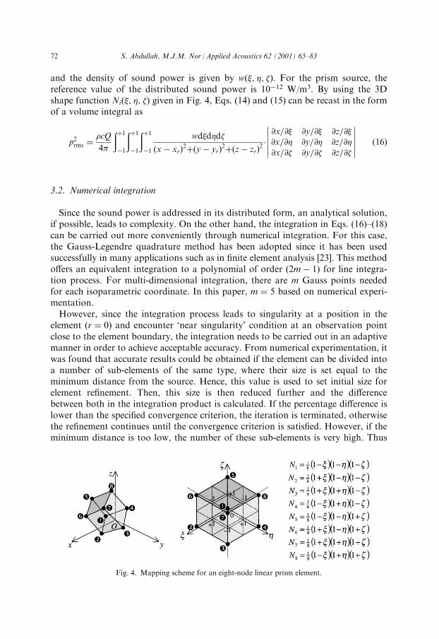
and the density of sound power is given by w �; �; �� . For the prism source, thereference value of the distributed sound power is 10ÿ12 W/m3. By using the 3Dshape function Ni �; �; �� given in Fig. 4, Eqs. (14) and (15) can be recast in the formof a volume integral as

p2rms ��cQ

4�

��1ÿ1

��1ÿ1

��1ÿ1

wd�d�d�

xÿ xr� �2� yÿ yr� �2� zÿ zr� �2 �@x=@� @y=@� @z=@�@x=@� @y=@� @z=@�@x=@� @y=@� @z=@�

�� 16�

3.2. Numerical integration

Since the sound power is addressed in its distributed form, an analytical solution,if possible, leads to complexity. On the other hand, the integration in Eqs. (16)±(18)can be carried out more conveniently through numerical integration. For this case,the Gauss-Legendre quadrature method has been adopted since it has been usedsuccessfully in many applications such as in ®nite element analysis [23]. This methodo�ers an equivalent integration to a polynomial of order (2mÿ 1) for line integra-tion process. For multi-dimensional integration, there are m Gauss points neededfor each isoparametric coordinate. In this paper, m � 5 based on numerical experi-mentation.However, since the integration process leads to singularity at a position in the

element (r � 0) and encounter `near singularity' condition at an observation pointclose to the element boundary, the integration needs to be carried out in an adaptivemanner in order to achieve acceptable accuracy. From numerical experimentation, itwas found that accurate results could be obtained if the element can be divided intoa number of sub-elements of the same type, where their size is set equal to theminimum distance from the source. Hence, this value is used to set initial size forelement re®nement. Then, this size is then reduced further and the di�erencebetween both in the integration product is calculated. If the percentage di�erence islower than the speci®ed convergence criterion, the iteration is terminated, otherwisethe re®nement continues until the convergence criterion is satis®ed. However, if theminimum distance is too low, the number of these sub-elements is very high. Thus

Fig. 4. Mapping scheme for an eight-node linear prism element.


for this case, the number of division is truncated to 103. By using this technique, thecalculated noise levels produced were very accurate even in the near ®eld, forexample an error less 0.2% at x=l � 0:0001 (see the next section for details).

3.3. Formula validations

The following sections describe the benchmarking aspects, which con®rm theaccuracy of the proposed algorithm. In these sections, the results from the proposedalgorithm for line and plane sources were validated and compared with those gen-erated using other methods in the literature. Also, it is worth noting that, in thiswork, the noise contours were produced by interpolating the data in logarithmicscale, instead linear scale as this type of interpolation is more appropriate for noiselevel contouring.

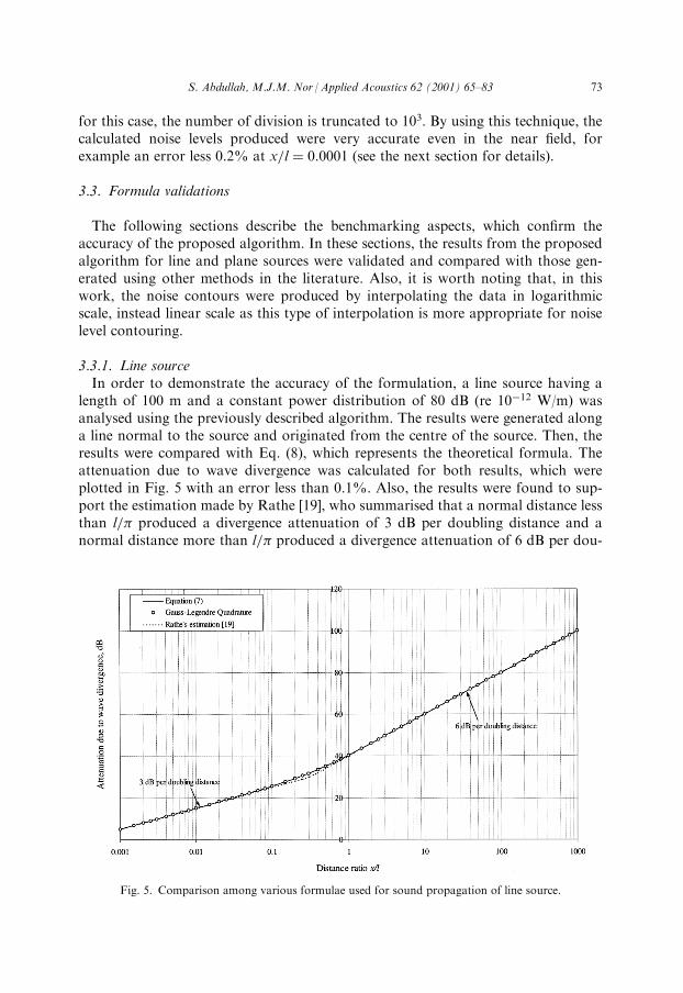
3.3.1. Line sourceIn order to demonstrate the accuracy of the formulation, a line source having a

length of 100 m and a constant power distribution of 80 dB (re 10ÿ12 W/m) wasanalysed using the previously described algorithm. The results were generated alonga line normal to the source and originated from the centre of the source. Then, theresults were compared with Eq. (8), which represents the theoretical formula. Theattenuation due to wave divergence was calculated for both results, which wereplotted in Fig. 5 with an error less than 0.1%. Also, the results were found to sup-port the estimation made by Rathe [19], who summarised that a normal distance lessthan l=� produced a divergence attenuation of 3 dB per doubling distance and anormal distance more than l=� produced a divergence attenuation of 6 dB per dou-

Fig. 5. Comparison among various formulae used for sound propagation of line source.


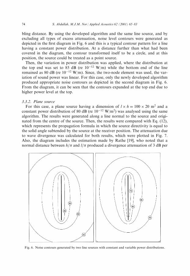
bling distance. By using the developed algorithm and the same line source, and byexcluding all types of excess attenuation, noise level contours were generated asdepicted in the ®rst diagram in Fig. 6 and this is a typical contour pattern for a linehaving a constant power distribution. At a distance further than what had beencovered in the diagram, the contour transformed itself to be a circle, and at thisposition, the source could be treated as a point source.Then, the variation in power distribution was applied, where the distribution at

the top end was set to 85 dB (re 10ÿ12 W/m) while the bottom end of the lineremained as 80 dB (re 10ÿ12 W/m). Since, the two-node element was used, the var-iation of sound power was linear. For this case, only the newly developed algorithmproduced appropriate noise contours as depicted in the second diagram in Fig. 6.From the diagram, it can be seen that the contours expanded at the top end due tohigher power level at the top.

3.3.2. Plane sourceFor this case, a plane source having a dimension of l� h � 100� 20 m2 and a

constant power distribution of 80 dB (re 10ÿ12 W/m2) was analysed using the samealgorithm. The results were generated along a line normal to the source and origi-nated from the centre of the source. Then, the results were compared with Eq. (12),which represents the propagation formula in which the source directivity is equal tothe solid angle subtended by the source at the receiver position. The attenuation dueto wave divergence was calculated for both results, which were plotted in Fig. 7.Also, the diagram includes the estimation made by Rathe [19], who noted that anormal distance between h=� and l=� produced a divergence attenuation of 3 dB per

Fig. 6. Noise contours generated by two line sources with constant and variable power distributions.


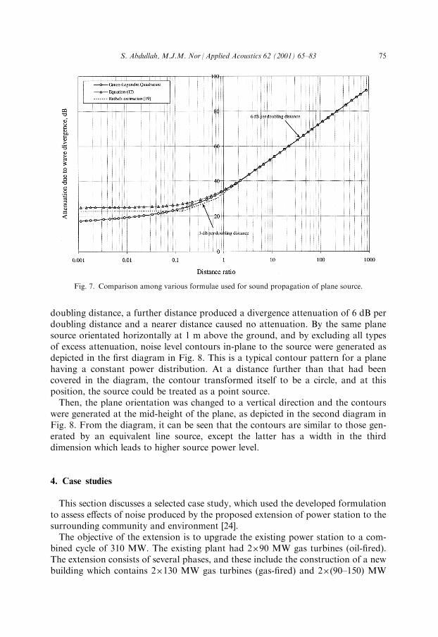
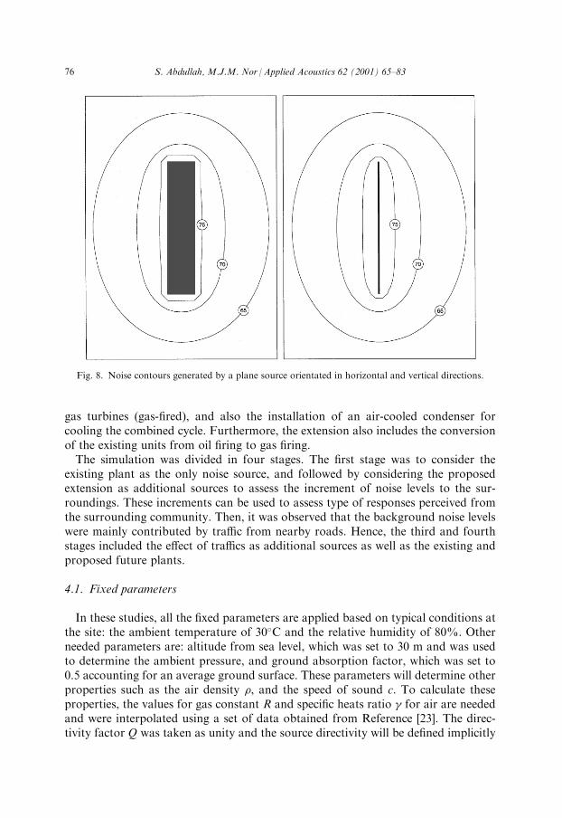
doubling distance, a further distance produced a divergence attenuation of 6 dB perdoubling distance and a nearer distance caused no attenuation. By the same planesource orientated horizontally at 1 m above the ground, and by excluding all typesof excess attenuation, noise level contours in-plane to the source were generated asdepicted in the ®rst diagram in Fig. 8. This is a typical contour pattern for a planehaving a constant power distribution. At a distance further than that had beencovered in the diagram, the contour transformed itself to be a circle, and at thisposition, the source could be treated as a point source.Then, the plane orientation was changed to a vertical direction and the contours

were generated at the mid-height of the plane, as depicted in the second diagram inFig. 8. From the diagram, it can be seen that the contours are similar to those gen-erated by an equivalent line source, except the latter has a width in the thirddimension which leads to higher source power level.

4. Case studies

This section discusses a selected case study, which used the developed formulationto assess e�ects of noise produced by the proposed extension of power station to thesurrounding community and environment [24].The objective of the extension is to upgrade the existing power station to a com-

bined cycle of 310 MW. The existing plant had 2�90 MW gas turbines (oil-®red).The extension consists of several phases, and these include the construction of a newbuilding which contains 2�130 MW gas turbines (gas-®red) and 2�(90±150) MW

Fig. 7. Comparison among various formulae used for sound propagation of plane source.


gas turbines (gas-®red), and also the installation of an air-cooled condenser forcooling the combined cycle. Furthermore, the extension also includes the conversionof the existing units from oil ®ring to gas ®ring.The simulation was divided in four stages. The ®rst stage was to consider the

existing plant as the only noise source, and followed by considering the proposedextension as additional sources to assess the increment of noise levels to the sur-roundings. These increments can be used to assess type of responses perceived fromthe surrounding community. Then, it was observed that the background noise levelswere mainly contributed by tra�c from nearby roads. Hence, the third and fourthstages included the e�ect of tra�cs as additional sources as well as the existing andproposed future plants.

4.1. Fixed parameters

In these studies, all the ®xed parameters are applied based on typical conditions atthe site: the ambient temperature of 30�C and the relative humidity of 80%. Otherneeded parameters are: altitude from sea level, which was set to 30 m and was usedto determine the ambient pressure, and ground absorption factor, which was set to0.5 accounting for an average ground surface. These parameters will determine otherproperties such as the air density �, and the speed of sound c. To calculate theseproperties, the values for gas constant R and speci®c heats ratio for air are neededand were interpolated using a set of data obtained from Reference [23]. The direc-tivity factor Q was taken as unity and the source directivity will be de®ned implicitly

Fig. 8. Noise contours generated by a plane source orientated in horizontal and vertical directions.


through variable distribution of sound power levels of shaped sources. Furthermore,since the simulation was done in three dimensions but the results were plotted in twodimensions, the contours were generated at a particular height, in this case at 1 mabove the ground.

4.2. Measurement of sound pressure levels

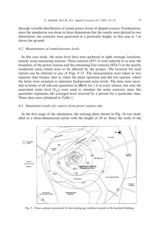
In this case study, the noise level data were gathered at eight strategic locations,namely noise measuring stations. Three stations (ST1-3) were selected in or near theboundary of the power station and the remaining four stations (ST4-7) in the nearbyresidential areas which were to be a�ected by the project. The location for eachstation can be referred to any of Figs. 9±12. The measurement were taken in twoseparate time frames, that is, when the plant operated and did not operate, wherethe latter were assumed to represent background noise levels. The data were recor-ded in forms of all relevant quantities in dB(A) for 1 h at every station, but only theequivalent noise level (Leq) were used to simulate the noise contours since thisquantities represents the averaged level received by a person for a particular time.These data were tabulated in Table 1.

4.3. Simulation results for sources from power station only

In the ®rst stage of the simulation, the existing plant shown in Fig. 10 was mod-elled as a three-dimensional prism with the height of 30 m. Since the walls of the

Fig. 9. Noise contours generated by the existing gas turbines located in the hatched building.


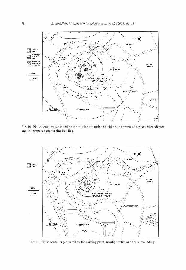
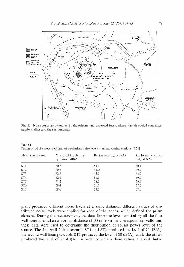
Fig. 11. Noise contours generated by the existing plant, nearby tra�cs and the surroundings.

Fig. 10. Noise contours generated by the existing gas turbine building, the proposed air-cooled condenser

and the proposed gas turbine building.


plant produced di�erent noise levels at a same distance, di�erent values of dis-tributed noise levels were applied for each of the nodes, which de®ned the prismelement. During the measurement, the data for noise levels emitted by all the fourwall were also taken a normal distance of 30 m from the corresponding walls, andthese data were used to determine the distribution of sound power level of thesource. The ®rst wall facing towards ST1 and ST2 produced the level of 79 dB(A),the second wall facing towards ST5 produced the level of 80 dB(A), while the othersproduced the level of 75 dB(A). In order to obtain these values, the distributed

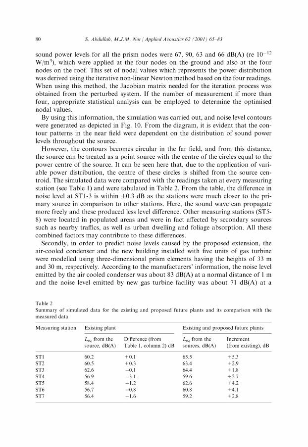
Fig. 12. Noise contours generated by the existing and proposed future plants, the air-cooled condenser,

nearby tra�cs and the surroundings.

Table 1

Summary of the measured data of equivalent noise levels at all measuring stations [8,24]

Measuring station Measured Leq during

operation, dB(A)

Background Leq, dB(A) Leq from the source

only, dB(A)

ST1 60.5 50.0 60.1

ST2 60.3 43..5 60.2

ST3 62.8 45.0 62.7

ST4 62.1 58.0 60.0

ST5 61.2 56.0 59.6

ST6 58.4 51.0 57.5

ST7 58.6 50.0 58.0


sound power levels for all the prism nodes were 67, 90, 63 and 66 dB(A) (re 10ÿ12

W/m3), which were applied at the four nodes on the ground and also at the fournodes on the roof. This set of nodal values which represents the power distributionwas derived using the iterative non-linear Newton method based on the four readings.When using this method, the Jacobian matrix needed for the iteration process wasobtained from the perturbed system. If the number of measurement if more thanfour, appropriate statistical analysis can be employed to determine the optimisednodal values.By using this information, the simulation was carried out, and noise level contours

were generated as depicted in Fig. 10. From the diagram, it is evident that the con-tour patterns in the near ®eld were dependent on the distribution of sound powerlevels throughout the source.However, the contours becomes circular in the far ®eld, and from this distance,

the source can be treated as a point source with the centre of the circles equal to thepower centre of the source. It can be seen here that, due to the application of vari-able power distribution, the centre of these circles is shifted from the source cen-troid. The simulated data were compared with the readings taken at every measuringstation (see Table 1) and were tabulated in Table 2. From the table, the di�erence innoise level at ST1-3 is within �0.3 dB as the stations were much closer to the pri-mary source in comparison to other stations. Here, the sound wave can propagatemore freely and these produced less level di�erence. Other measuring stations (ST5-8) were located in populated areas and were in fact a�ected by secondary sourcessuch as nearby tra�cs, as well as urban dwelling and foliage absorption. All thesecombined factors may contribute to these di�erences.Secondly, in order to predict noise levels caused by the proposed extension, the

air-cooled condenser and the new building installed with ®ve units of gas turbinewere modelled using three-dimensional prism elements having the heights of 33 mand 30 m, respectively. According to the manufacturers' information, the noise levelemitted by the air cooled condenser was about 83 dB(A) at a normal distance of 1 mand the noise level emitted by new gas turbine facility was about 71 dB(A) at a

Table 2

Summary of simulated data for the existing and proposed future plants and its comparison with the

measured data

Measuring station Existing plant Existing and proposed future plants

Leq from the

source, dB(A)

Di�erence (from

Table 1, column 2) dB

Leq from the

sources, dB(A)

Increment

(from existing), dB

ST1 60.2 +0.1 65.5 +5.3

ST2 60.5 +0.3 63.4 +2.9

ST3 62.6 ÿ0.1 64.4 +1.8

ST4 56.9 ÿ3.1 59.6 +2.7

ST5 58.4 ÿ1.2 62.6 +4.2

ST6 56.7 ÿ0.8 60.8 +4.1

ST7 56.4 ÿ1.6 59.2 +2.8


normal distance of 30 m. The predicted level for the new facility is much lower thanthat experienced in the existing plant since the new gas-®red units operated quieterthan the existing units, which were oil-®red. By assuming a constant sound powerdistribution, the distributed sound power levels were speci®ed as 67.4 dB(A) and 75dB(A) (re 10ÿ12 W/m3) for the air cooled condenser and the new gas turbines facil-ity, respectively. Then, the simulation was carried out and noise level contours weregenerated as depicted in Fig. 10. The summary of the increment of noise levels foreach measuring station was tabulated in Table 2. From these table, it was found thatthe noise levels at all stations were generally higher than the existing levels and thedi�erences were logarithmically proportional to the mean distance from the de®nedsources.

4.4. Simulation results for sources from power station and road tra�cs

In the third stage of the simulation, background noise was included so that theactual noise contours for the whole area of study can be produced. From Table 1,the background noise levels were varied for every measuring station, and it wasobserved that the main source of background noise was nearby road tra�cs. Others,which came from the surroundings, such as peoples, river ¯ow, birds, trees andwinds, were considered to be very minimal. Furthermore, even though the area ofstudy also has railway tracks, noise from passing trains was not considered heresince the frequency of the train passing across the area of study was very low. Allthese minor factors were combined to form a ¯oor value for noise levels. In thisstudy, the ¯oor value was taken as equal to 45 dB(A), that is, the background noiseat ST3, since this location was very remote and thus the background noise wasalmost purely attributed from all these minor e�ects.In order to derive the suitable distribution of sound power level for tra�cs, the

reading at ST4 was taken as a reference since this station was the closest to the mainroad and across the bridge. By assuming constant tra�c ¯ow, it was found that thesuitable value was 83.4 dB(A) (re 10ÿ12 W/m) for main road. Also, by assuming thatthe smaller road was half of those speci®ed for main roads, the distribution of soundpower level for smaller roads was set at 80.4 dB(A) (re 10ÿ12 W/m). Since the roadwidth was generally too small in comparison with the area of study, these curvytra�cs can be modelled using piecewise line elements. Hence, the simulation wascarried out for the existing source and the tra�cs, and the noise level contours areillustrated in Fig 11. The simulated data were again compared with the readingstaken at every measuring station (see Table 1) and were tabulated in Table 3. Themean di�erence shown in Table 3 was found higher than the mean di�erence illu-strated in Table 1. This was due to inconsistency of noise sources occurred at dif-ferent time frames selected during the measurement of noise levels when the existingplant operated and the measurement of background noise levels. However, thissimulation can be accepted to represent the real scenario since the overall level dif-ference is less than �1.2 dB.Lastly, in the fourth stage of the simulation, all the existing and proposed future

plants were combined with the source from tra�cs and the background noise levels


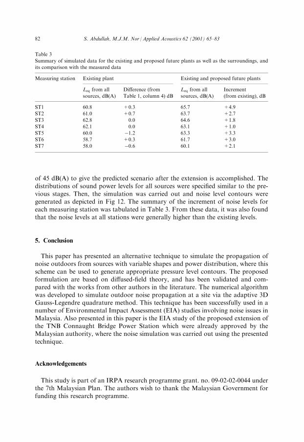
of 45 dB(A) to give the predicted scenario after the extension is accomplished. Thedistributions of sound power levels for all sources were speci®ed similar to the pre-vious stages. Then, the simulation was carried out and noise level contours weregenerated as depicted in Fig 12. The summary of the increment of noise levels foreach measuring station was tabulated in Table 3. From these data, it was also foundthat the noise levels at all stations were generally higher than the existing levels.

5. Conclusion

This paper has presented an alternative technique to simulate the propagation ofnoise outdoors from sources with variable shapes and power distribution, where thisscheme can be used to generate appropriate pressure level contours. The proposedformulation are based on di�used-®eld theory, and has been validated and com-pared with the works from other authors in the literature. The numerical algorithmwas developed to simulate outdoor noise propagation at a site via the adaptive 3DGauss-Legendre quadrature method. This technique has been successfully used in anumber of Environmental Impact Assessment (EIA) studies involving noise issues inMalaysia. Also presented in this paper is the EIA study of the proposed extension ofthe TNB Connaught Bridge Power Station which were already approved by theMalaysian authority, where the noise simulation was carried out using the presentedtechnique.

Acknowledgements

This study is part of an IRPA research programme grant. no. 09-02-02-0044 underthe 7th Malaysian Plan. The authors wish to thank the Malaysian Government forfunding this research programme.

Table 3

Summary of simulated data for the existing and proposed future plants as well as the surroundings, and

its comparison with the measured data

Measuring station Existing plant Existing and proposed future plants

Leq from all

sources, dB(A)

Di�erence (from

Table 1, column 4) dB

Leq from all

sources, dB(A)

Increment

(from existing), dB

ST1 60.8 +0.3 65.7 +4.9

ST2 61.0 +0.7 63.7 +2.7

ST3 62.8 0.0 64.6 +1.8

ST4 62.1 0.0 63.1 +1.0

ST5 60.0 ÿ1.2 63.3 +3.3

ST6 58.7 +0.3 61.7 +3.0

ST7 58.0 ÿ0.6 60.1 +2.1


References

[1] Anderson GS, Kurze UJ. Outdoor sound propagation. In: Beranek LL, VeÂ r IL, editors. Noise and

vibration control engineering Ð principles and applications, New York: John Wiley & Sons, 1992.

[2] Piercy JE, Embleton TFW, Sutherland LC. Review of noise propagation in the atmosphere. Journal

of the Acoustical Society of America 1977;61:1403±18.

[3] Delany ME. Sound propagation in the atmosphere: a historical review. Proceedings of the Institution

of Acoustics 1978;1:32±72.

[4] Embleton TFW. Sound propagation outdoors: improved prediction schemes for the 80's. Noise

Control Engineering 1982;18:30±9.

[5] Harris CW. Handbook of noise control. 2nd Ed. New York: McGraw-Hill, 1979.

[6] ISO/DIS 9613-2. Acoustics: attenuation of sound during propagation outdoors Ð part 2 (Draft

Standard), International Organisation for Standardisation, Geneva, 1995.

[7] Bies DA, Hansen CH. Engineering noise control Ð theory and practice. 2nd Ed. London: E & FN

Spon, 1996.

[8] Mohd Nor MJ, Abdullah S. Development of noise assessment software (NAS). In: Proceedings of

MINDEX/SIRIM '92, Kuala Lumpur, Malaysia, Aug. 1992.

[9] Chambers C. Speci®cation Nos. NWG-1, NWG-2, NWG-3 (Revision 1), Oil Companies Materials

Association, London, 1972.

[10] Jenkins RH, Johnson JB. The assessment and monitoring of the contribution from a large petro-

chemical complex to neighbourhood noise levels. Noise Control Vibration and Insulation:328±35

[11] Sutton P. Process noise: evaluation and control. Applied Acoustics 1976;9:17±38.

[12] Tonin R. Estimating noise levels from petrochemical plants, mines and industrial complexes.

Acoustics Australia 1985;13:59±67.

[13] Marsh KJ. Speci®cation and prediction of noise levels in oil re®neries and petrochemical plants.

Applied Acoustics 1976;9:1±15.

[14] Marsh KJ. The CONCAWE model for calculating the propagation of noise from open air industrial

plants. Applied Acoustics 1982;15:411±28.

[15] Allen JB, Berkeley DA. Image method for e�ciently simulating small-room acoustics. Journal of the

Acoustical Society of America 1979;65:943±50.

[16] Borish J. Extension of the image model to arbitrary polyhedra. Journal of the Acoustical Society of

America 1984;75:1827±36.

[17] Krokstad A, Strom S, Sorsdal S. Calculating the acoustical room response by the use of a ray-tracing

technique. Journal of Sound and Vibration 1968;8:118±25.

[18] Ondet AM, Barbry JL. Modelling of sound propagation in ®tted workshops using ray tracing.

Journal of the Acoustical Society of America 1989;85:787±96.

[19] Rathe EJ. Note on two common problems on sound propagation. Journal of Sound and Vibration

1969;10:472±9.

[20] Hohenwarter D. Noise radiation of (rectangular) plane sources. Applied Acoustics 1991;33:45±62.

[21] Sutherland LC, Piercy JF, Bass HE, Evans LB. Method for calculating the absorption of sound by

the atmosphere. Journal of the Acoustical Society of America, 1974; 56 (Suppl. 1) (abstract).

[22] Zienkiewicz OC, Taylor RL. The ®nite element method (Vol. I Ð basic formulation). 4th Ed. Lon-

don: McGraw-Hill, 1989.

[23] Perry RH, Green DW, Maloney JO. Perry's chemical engineers' handbook. 6th Ed. New York:

McGraw-Hill, 1984.

[24] Tenaga Nasional Berhad. Environmental inpact assessment: proposed extension Connaught Bridge

power station, Klang, Selangor Darul Ehsan. Bureau of Research and Consultancy, National Uni-

versity of Malaysia, June 1991.


The utilisation of an adaptive 3D Gauss-Legendre quadrature in the simulation of sound propagation outdoors for sources with variable power distribution

Documents