The use of electrical resistivity tomography (ERT) to ...

Scholars' Mine Scholars' Mine

Masters Theses Student Theses and Dissertations

Spring 2012

The use of electrical resistivity tomography (ERT) to delineate The use of electrical resistivity tomography (ERT) to delineate

water-filled vugs near a bridge foundation water-filled vugs near a bridge foundation

Jeremiah Chukwunonso Obi

Follow this and additional works at: https://scholarsmine.mst.edu/masters_theses

Part of the Geological Engineering Commons

Department: Department:

Recommended Citation Recommended Citation Obi, Jeremiah Chukwunonso, "The use of electrical resistivity tomography (ERT) to delineate water-filled vugs near a bridge foundation" (2012). Masters Theses. 5146. https://scholarsmine.mst.edu/masters_theses/5146

This thesis is brought to you by Scholars' Mine, a service of the Missouri S&T Library and Learning Resources. This work is protected by U. S. Copyright Law. Unauthorized use including reproduction for redistribution requires the permission of the copyright holder. For more information, please contact [email protected].

https://library.mst.edu/

https://library.mst.edu/

https://scholarsmine.mst.edu/

https://scholarsmine.mst.edu/masters_theses

https://scholarsmine.mst.edu/student-tds

https://scholarsmine.mst.edu/masters_theses?utm_source=scholarsmine.mst.edu%2Fmasters_theses%2F5146&utm_medium=PDF&utm_campaign=PDFCoverPages

http://network.bepress.com/hgg/discipline/1400?utm_source=scholarsmine.mst.edu%2Fmasters_theses%2F5146&utm_medium=PDF&utm_campaign=PDFCoverPages

https://scholarsmine.mst.edu/masters_theses/5146?utm_source=scholarsmine.mst.edu%2Fmasters_theses%2F5146&utm_medium=PDF&utm_campaign=PDFCoverPages

mailto:[email protected]

i

i

THE USE OF ELECTRICAL RESISTIVITY TOMOGRAPHY (ERT) TO DELINEATE

WATER-FILLED VUGS NEAR A BRIDGE FOUNDATION

by

JEREMIAH CHUKWUNONSO OBI

A THESIS

Presented to the Faculty of the Graduate School of the

MISSOURI UNIVERSITY OF SCIENCE AND TECHNOLOGY

In Partial Fulfillment of the Requirements for the Degree

MASTER OF SCIENCE IN GEOLOGICAL ENGINEERING

2012

Approved by

Neil Anderson, Advisor

David J. Rogers

Leslie Gertsch

ii

2012

Jeremiah Chukwunonso Obi

All Rights Reserved

iii

ABSTRACT

A structural support was needed to strengthen the load-bearing capacity of an

unnamed bridge foundation in Laclede County in South-Central Missouri due to

increasing traffic volume and age of the bridge. This area is characterized by karstic

features such as losing streams, underground caves and sinkholes. During the

construction of a drilled shaft for the substructure, a few feet north of the north footing of

the pier, voids were noted beneath a roughly 2 foot thick cap of dolomite rock. Because

of this, there were concerns about the integrity of the rock beneath the existing bridge

foundation.

Consequently, subsurface investigation was conducted at the site using borings.

Results from the borings confirmed the presence of voids adjacent to or at the foundation

bearing level of the northern and central pier footings. This information alone provides

accurate data only at the sampling location, so control elsewhere has to be interpolated,

which can result in erroneous interpretation. To map the lateral and vertical extent of the

voids, electrical resistivity tomography (ERT) was employed using the SuperSting R8/IP

Earth resistivity meter. The result obtained was used to complement the borehole

information. Dipole-dipole electrode configuration was used. Based on the interpretation

of the results of the ERT survey and borehole control, it was concluded that the bedrock

in the area was mainly dolomite dipping from east to west, and appears to be competent

bedrock. Voids encountered were not of room-sizes as to breach the integrity of the

bridge foundation. Compaction grouting was the engineering solution employed to fill the

voids and stabilize the ground around the structure.

iv

ACKNOWLEDGEMENTS

My immense gratitude goes to Dr. Neil Anderson, my advisor for his invaluable

contribution towards the success of this thesis. He directed and encouraged me to take up

this topic. I also thank Dr. David J. Rogers and Dr. Leslie Gertsch for accepting to be on

my committee. Their insightful comments and suggestions were great.

My special thanks go to my family and friends for their unflinching support and

encouragement throughout my graduate studies.

v

TABLE OF CONTENTS

Page

ABSTRACT .................................................................................................................. iii

ACKNOWLEDGMENTS ............................................................................................. iv

LIST OF ILLUSTRATIONS ........................................................................................ vii

LIST OF TABLES ........................................................................................................ ix

SECTION

1. INTRODUCTION ...................................................................................................1

1.1. OBJECTIVE ....................................................................................................1

1.2. SITE DESCRIPTION ......................................................................................2

2. GEOLOGIC OVERVIEW OF STRATIGRAPHIC UNITS IN LACLEDE

COUNTY, MISSOURI ...........................................................................................5

2.1. BEDROCK DISTRIBUTION IN THE AREA .................................................6

2.1.1. Ordovician System .................................................................................6

2.1.2. Canadian Series .....................................................................................7

2.1.2.1. Gasconade formation ................................................................ 7

2.1.2.2. Roubidoux formation . .............................................................. 8

2.1.2.3. Jefferson City formation … ....................................................... 8

2.1.2.4. Cotter formation ....................................................................... 9

2.2. SURFICIAL MATERIALS IN LACLEDE COUNTY, MISSOURI ................9

2.3. FAULTING .................................................................................................. 10

3. THEORY OF KARST FORMATION .................................................................. 11

4. GEOPHYSICAL APPLICATION ......................................................................... 16

4.1. GEOPHYSICAL TOOLS USED TO MAP VOIDS AND CAVES ................ 17

4.1.1. Ground Penetrating Radar (GPR) Method ............................................ 17

4.1.2. Gravity Method .................................................................................... 17

4.1.3. Electromagnetic Method (EM) ............................................................. 18

4.1.4. Seismic Reflection Method .................................................................. 18

4.1.5. Electrical Resistivity Tomography Method........................................... 19

vi

5. LITERATURE REVIEW: ELECTRICAL RESISTIVITY

TOMOGRAPHY (ERT) ........................................................................................ 20

5.1. CURRENT FLOW IN THE SUBSURFACE ................................................. 21

5.2. RELATIONSHIP BETWEEN GEOLOGY AND RESISTIVITY .................. 22

5.3. OHM'S LAW AND RESISTIVITY ............................................................... 23

5.4. THEORETICAL DETERMINATION OF RESISTIVITY ............................. 24

5.5. APPARENT RESISTIVITY .......................................................................... 28

5.6. ELECTRICAL RESISTIVITY ARRAY CONFIGURATION ........................ 30

5.7. 2-D RESISTIVITY ARRAYS ........................................................................ 30

6. DATA ACQUISITION ......................................................................................... 34

6.1. EQUIPMENT USED FOR ERT ……….....………………………………….38

6.2. ELECTRICAL RESISTIVITY TOMOGRAPHY DATA PROCESSING ...... 40

6.3. RESOLUTION LIMITATION OF ERT METHOD ....................................... 47

7. DATA INTERPRETATION ................................................................................. 49

7.1. GENERAL GUIDE TO ERT DATA INTERPRETATION ............................ 50

7.2. ENGINEERING SOLUTION APPLIED ....................................................... 58

8. CONCLUSION ..................................................................................................... 61

BIBLIOGRAPHY ......................................................................................................... 63

VITA ............................................................................................................................ 65

vii

LIST OF ILLUSTRATIONS

Figure Page

1.1. Location of the project site in Laclede County, Missouri. ..........................................3

1.2. Data acquisition of ERT at the site and the nature of the site .....................................4

2.1. Fault pattern in southwestern Missouri (geosphere.gsapubs.org) ............................. 10

3.1. Karst map of the US published by AGI (Veni et al., 2001) ...................................... 11

3.2. Stages of sinkhole formation ................................................................................... 14

3.3. Nature of a fully developed sinkhole (http://news.nationalgeographic.com) ............ 15

3.4. Karst feature near bridge pier at the project site. ...................................................... 15

5.1. Electric circuit for illustration of Ohm’s Law. ......................................................... 24

5.2. Current lines radiating from the source and converging on the sink electrodes…….25

5.3.Current lines and equipotential surfaces in a medium of uniform resistivity ............. 27

5.4. Current electrodes A and B and potential electrodes M and N ................................. 28

5.5. The most common electrode array configurations ................................................... 31

6.1. Data acquisition of profile 1 .................................................................................... 34

6.2. Data acquisition of profile 2 .................................................................................... 35

6.3. Data acquisition of profile 5. ................................................................................... 35

6.4. Sketch of electrical resistivity traverses at project site. ............................................ 36

6.5. General site plan .................................................................................................... 37

6.6. Earth resistivity meter-SuperSting R8/IP, product of Advanced Geosciences Inc.. .. 39

6.7. Electrical resistivity dipole-dipole array configuration used in the field ................... 39

6.8. Example of a data set with a few bad data points (Loke, 2004). ............................... 41

6.9. Arrangement of the blocks used in a model together with the data points. ............... 42

viii

6.10. Unedited/raw profile 1 .......................................................................................... 43





7.1. Interpreted profile 1 ................................................................................................ 52





7.6. Lineament showing horizontal bedding plane.......................................................... 60

ix

LIST OF TABLES

Table Page

2.1. Geologic and stratigraphic units in Laclede County (Vandike, 1993) ....................5

5.1. Resistivity of common Earth’s materials (Robinson, 1988) ................................ 22

7.1. Summary of results of boring logs at the project site .......................................... 50

7.2. Summary of sizes of voids and volume of grout used to seal the voids ............... 58

1

1. INTRODUCTION

1.1. OBJECTIVE

A structural support was needed to support an unnamed bridge foundation located

in Laclede County in South-Central Missouri. The purpose for the construction of this

structural support for the existing bridge was to strengthen the load bearing capacity of

the bridge due to increasing volume of traffic and age of the bridge.

During the construction of a drilled shaft for the substructure, a few feet north of

the footing of the pier 6, voids were noted beneath a roughly 2-foot-thick cap of dolomite

rock. Because of this, there were concerns about the integrity of the rock beneath the

existing bridge foundation. Background information obtained from borings confirmed the

presence of voids adjacent to or at the foundation bearing level of the northern and

central pier footings.

The geophysical laboratory at the Missouri University of Science and Technology

(MS&T) was contracted to carry out a geophysical investigation of the project site to map

the lateral and vertical extent of the voids detected near the pier. The result of the

investigation had to be compared with the existing boring results for ground truth. This

would ensure that subsurface conditions that would affect the integrity of the bridge

foundation were detected and proper engineering solution such as compaction grouting

employed.

With this task in mind, electrical resistivity tomography (ERT) method was

deemed the appropriate geophysical tool to be employed for this project because it has

proven to be an effective tool in mapping hidden karst features especially in areas with

2

highly variable elevation of bedrock. Data acquisition using electrical resistivity

tomography is automated. The interpretations are normally highly reliable if constrained

with borehole data. Also, proper use of this technique for karstic voids can often help

geotechnical engineers develop an effective program of test borings and grouting, since if

the bore spacing is greater than the cavity dimensions, it is possible to miss the cavity

completely. Bedrock voids, whether filled with air, water, or sediment, constitute

“missing mass” in comparison to solid rocks.

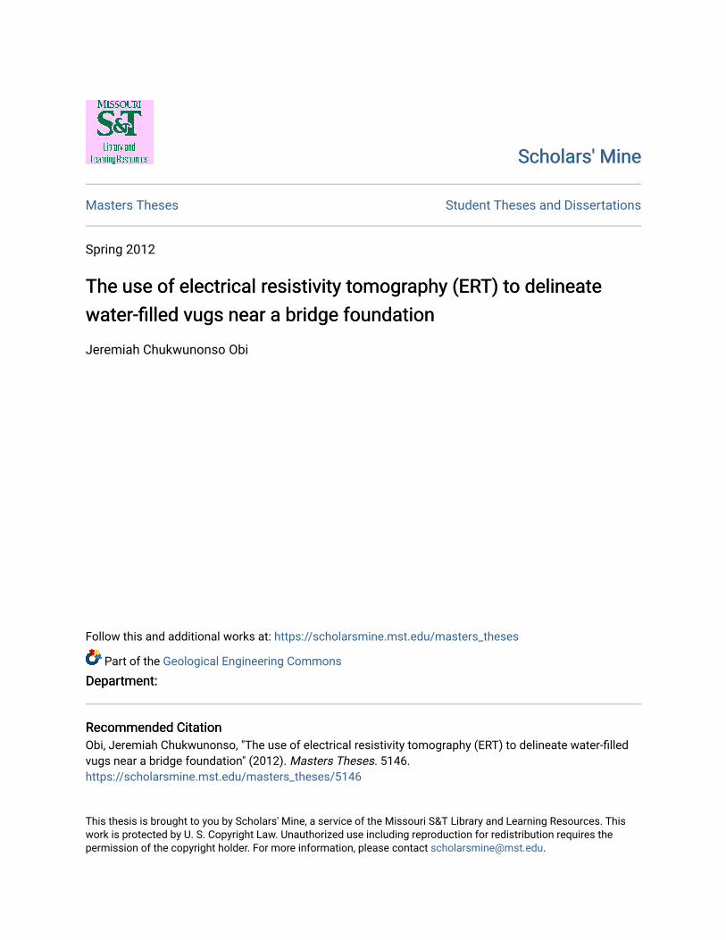
1.2. SITE DESCRIPTION

The project site is located in Laclede County, South-Central Missouri. It is part of

the Ozark Highland Area. The area is known for the development of karstic feautures

such as caves, springs, and sinkholes. The sinkholes that frequently develop on the broad,

prairie-like uplands vary from broad bowl-shaped depressions encompassing several

acres to steep-walled pits over 50 feet (15.2m) deep and 400 feet (121.9m) wide .

The area is underlain by sedimentary rocks of Ordovician age, namely the

Gasconade Formation, the Roubidoux Formation, Jefferson City Formation and Cotter

Formation. The Gasconade Formation is overlain by the Roubidoux Formation which is

overlain by the Jefferson City Formation that caps the upland in the project site. These

sedimentary strata are generally flat-lying. There is an area where the sloping valley floor

intercepts the Gasconade Formation directly upstream of the project site. The Gasconade

Formation is predominantly light brownish cherty dolomite, and consists of upper

Gasconade dolomite and lower Gasconade dolomite.

3

The Roubidoux Formation consists of dolomite, cherty dolomite, sandy dolomite and

dolomitic sandstone.

The Jefferson City Formation consists primarily of medium to finely-crystalline

dolomite. The location of the project site is shown in Figure 1.1.

Figure 1.1. Location of the project site in Laclede County, Missouri

The project site is underlain mainly by the Gasconade Formation (Lower

Gasconade Dolomite and Upper Gasconade Dolomite) and Roubidoux Formation,

according to information from literature and types of rocks and rock samples collected

from the site. The project site has an undulating topography with majority of the sloped

Location

4

areas covered with grasses, shrubs and trees. The area is covered mostly by alluvium;

weathered or eroded particles of minerals which are transported by a river and deposited

usually temporarily at points along the flood plain of a river. The alluvium consists of

chert gravels and cobbles interbeded with clay, silt, and sand. The cherty residuum is

developed from weathering of dolomite, chert and sandstone. This type of geologic

formation (Figure 1.2) is prone to sinkholes, losing streams, caves, and springs.

Figure 1.2. Data acquisition of ERT at the site and the nature of the site

5

2. GEOLOGIC OVERVIEW OF STRATIGRAPHIC UNITS IN LACLEDE

COUNTY, MISSOURI

The geologic overview of the stratigraphic units in Laclede County, Missouri

presented here is based on work of Martin, et al. (1961). The geologic and stratigraphic

units of the study area belong to the Ordovician System and specifically the Canadian

series as presented in Table 2.1.

Table 2.1. Geologic and stratigraphic units in Laclede County (Vandike, 1993)

System Series Group Formation Regional

Thickness

(ft.)

Mis

siss

ippia

n

Osa

gea

n Burlington-Keokuk Formation 150-270

Elsey Formation 25-75

Reeds-Spring Formation 125

Pierson Formation 90

Kin

der

hookia

n

Choute

au Northview Formation 5-80

Compton Formation 30

Ord

ovic

ian

Can

adia

n

Cotter Formation

600 Jefferson-City Formation

Rubidoux Formation 150

Gas

conad

e F

orm

atio

n Upper Gasconade Dolomite

350

Lower Gasconade Dolomite

Gunter Sandstone Member

25

6

Table 2.1. Cont’d. Geologic and stratigraphic units in Laclede County (Vandike, 1993)

System

Series

Group Formation Thickness (ft.)

Cam

bri

an

Upper

Eminence Formation

500 Potosi Formation

Elv

is

Derby-Doerun Formation

Davis Formation 150

System Series Group Formation

Thickness

(ft.)

Bonneterre Formation 200

Lamotte Formation 150

Precambrian Crystalline rock

2.1. BEDROCK DISTRIBUTION IN THE AREA

The geologic and stratigraphic succession in Missouri presented here is based on

the work of James A. Martin, Robert D. Knight, and William C. Hayes, “The

Stratigraphic succession in Missouri”, 1961. The project site belongs to Ordovician

System and Canadian Series and is described as follows:

2.1.1. Ordovician System. Rocks of Ordovician age are exposed over

approximately one-third of the state of Missouri and attain aggregate thickness of

approximately 3,800 feet (1158.2m). They crop out chiefly in the southern, eastern, and

central parts of the state where they lie around the flanks of the Ozark Dome, sloping

downward from the center in all directions. There are unconformities at both the base and

the top of the system, with many significant unconformities being recognized as series

and stage boundaries within the system. There are Canadian Series, the Champlainian

Series, and Cincinnatian Series in the state that make up the Ordovician System. The

7

Canadian Series is one of the most extensive series represented in the state. The project

site belongs mainly to the Canadian Series.

2.1.2. Canadian Series. The rocks of the Canadian Series in Missouri are

principally arenaceous and consist of cherty dolomite and sandstone. They immediately

underlie the surface in a large part of the state south of the Missouri River. They are

bounded at the base and top by regional unconformities. Four bedrock Formations are

present in this series; all of them represent the Canadian Series of the Ordovician System

of Paleozoic Era. The bedrock formations, from oldest (lowest) to youngest, are

described as follows, based on reconnaissance mapping by Middendorf and Thompson

(1987) and Duley et al.1992).

2.1.2.1. Gasconade formation. The Gasconade is predominantly a light

brownish-gray, cherty dolomite. There is also a persistent sandstone unit in its lowest part

that is called the Gunter Member. The Gasconade Dolomite is typically light gray in

color, medium to coarsely - crystalline, thin to thick - bedded, cherty dolomite, and is

divisible into two units. The upper unit is a massively-bedded and relatively chert-free

dolomite that forms bluffs and pinnacle glades. It is medium to coarsely crystalline, and

weathers to a coarsely-pitted surface. It contains brown chert nodules or stringers with

some druses. Thickness of the upper unit ranges from 40 to 70 feet (12.2 to 21.3m). The

lower unit contains 30 to 50 percent chert and is light gray, medium-to coarsely

crystalline dolomite with thin beds or nodules of white to gray porcelaneous chert and

thin beds of silicified oolites. Cryptozoan reef structures are common and the top of the

lower part is marked by a persistent, locally silicified cryptozoan reef 2 to 8 feet (0.6 to

2.4m) thick. The formation is about 300 to 350 feet (91.4 to 106.7m) thick, but in the

8

project area, only the upper 50 to 100 feet (15.2 to 30.4 m) are exposed in valleys

bordering major rivers.

2.1.2.2. Roubidoux formation. The Roubidoux formation consists of sandstone,

dolomitic sandstone, and cherty dolomite. The sandstone is composed of fine-to medium-

grained quartz sand which characteristically is sub rounded and frosted. Gray and brown

colors are predominant on weathered surfaces, but the color of the fresh sandstone is

commonly light yellow, tan, or red at the surface and white in the subsurface. The

dolomite in the Roubidoux Formation is finely crystalline, light gray to brown in color,

and thinly to thickly bedded. Individual beds contain brown to gray, banded, oolitic,

sandy chert. White to dark-gray or brown chert is present as irregular layers, nodules, and

lenses in the dolomite. Cryptozoan reef structures are present locally as concentrically

banded chert masses up to 2 feet (0.6m) in diameter. Near the basal contact, brecciated

chert masses weather to boulders and blocks. The unit is about 120 to 150 feet (36.6 to

45.7m) thick.

2.1.2.3. Jefferson City formation. The Jefferson City formation is composed

principally of light brown to brown, medium to finely crystalline dolomite and

argillaceous dolomite. It typically contains banded chert nodules or thin seams of white to

light-gray chert with some generally discontinuous lenses of shale and fine-to medium

grained, poorly sorted white to light-gray sandstones up to 6 inches (0.15m) thick. A

persistent marker bed, 15 to 20 feet (4.6 to 6m) thick, of brown and gray-mottled,

medium-crystalline, thick-bedded dolomite weathers to a distinctive coarsely-pitted

ledge. This occurs about 30 feet (9.1m) above the base. The thickness of the Jefferson

9

City Formation ranges from 125 to 350 feet (38.1 to 106.7m); its average thickness is

about 200 feet (61m).

2.1.2.4. Cotter formation. The Cotter formation is composed mainly of light gray

to light brown, medium to finely crystalline, cherty dolomite. It contains thin

intercalated beds of green shale and sandstone. It is normally medium to thinly

bedded.

2.2. SURFICIAL MATERIALS IN LACLEDE COUNTY, MISSOURI

Surficial materials are defined as all solid earth materials (clay, silt, sand, gravel

and boulders) between the land surface and the top of bedrock (Vandike et al. 1992). In

the project area, the dominant surficial material is residuum, a product formed from the

disintegration and decomposition of Ordovician-age cherty dolomite and sandstone from

Gasconade Formation. Other surficial materials in this area are

loess; wind-deposited, clayey silt.

colluvium; sediment eroded and transported down slope by gravitational forces,

lag gravel; an accumulation of stones on an old surface from which the clay

matrix has been eroded.

alluvium; waterborne sediments of clay, silt, sand and gravel deposited in stream

channels and flood plains.

On the uplands, a composite surficial material profile consists of a thin layer of

loess on the surface, underlain by colluvium, lag gravel, residuum, and bedrock. The

distribution and thickness of surficial materials are controlled by topography, weathering,

erosion, and bedrock.

10

2.3. FAULTING

A distinctive pattern of faults crosses the area in a northwesterly trend; a less

well-defined series of faults crosses in a northeasterly trend (Vandike et al. 1992). The

faults have been inactive for millions of years, but weathering of bedrock along them has

produced a pattern of northwest-trending, solution-enlarged joints and fractures that may

control groundwater movement. Many of the river and creek channels have also

developed a northwesterly trend that reflects the primary fault direction. The Reelfoot

fault is the fault that trends northwest across the area as shown by black lines in Figure

2.1.

Figure 2.1. Fault pattern in southwestern Missouri (geosphere.gsapubs.org)

11

3.THEORY OF KARST FORMATION

The general representation of U.S. Karst areas published by American geological

institute (AGI) (Veni et. al., 2001) indicates that almost all southern Missouri is underlain

by carbonate rocks and recognized as a Karst terrain (shown in green color with star

symbol on the map, Figure 3.1).

Figure 3.1. Karst map of the US published by AGI (Veni et al., 2001)

Missouri

12

Karst is a term used to describe areas where the dissolving of soluble bedrock by

groundwater and surface water has played a dominant role in developing topographic and

drainage features. Karst features include sinkholes, losing streams, caves and springs.

Sinkholes are bowl-shaped depressions in the landscape resulting from solutional activity

underground.

Carbonate rocks (limestone and dolostone) are predominantly composed of calcite

mineral (CaCO3) and dolomite mineral (CaMg (CO3)2), and both, especially calcite,

dissolve in slightly acidic waters; the dissolved materials, along with the remaining

insoluble parts of the rock, are transported from the site through solution enlarged

openings in the bedrock. Over time, a void or opening develops in the shallow subsurface

that enlarges to the point where its roof can no longer sustain its own weight, and a

collapse occurs. If the void develops mostly in surficial materials and not bedrock, the

resulting sinkhole will initially have nearly vertical or overhung sides with little or no

bedrock exposed in the walls.

These materials are eroded by run-off from rainfall, eroding materials from the

rim of the sinkhole to form typical bowl-shaped depressions. In some cases the collapse

occurs within a cave passage or void developed in bedrock. In this case the shape of the

resulting sinkhole is more dependent on the configuration of the bedrock void. The

sinkhole may contain vertical bedrock walls along parts or all of its perimeter, and may

contain an enterable cave passage. The vast majority of sinkholes in the study area and

its environs are developed in surficial materials, and few have bedrock walls. Sinkholes

can be found in any of the four geologic formations exposed in this area, but are most

13

commonly developed in deeply-weathered Roubidoux Formation and Jefferson City

Dolomite.

Stages of sinkhole formation are illustrated in Figure 3.2. The illustration is

conceptual, meaning that actual conditions in nature may vary. For instance, the rock and

soil layers may be thicker or thinner, the fractures and cave passages may be larger or

smaller, and surfaces are likely to be much more irregular in shape. The stages are

described as follows (www.dnr.mo.gov/.../geores/sinkholeformation.htm):

Stage 1 –The opening in the bedrock surface allows overlying soil to move

downwards into a cave passage. In this case the solution-widened fracture in the

bedrock is choked with soil.

Stage 2 – The collected soil from stage one is carried away by flowing water.

Stage 3 – Soil in the fracture or bedrock opening collapses into the cave or is

washed into the cave by water movement from the soil into the cave.

Stage 4 – Voids form at the bedrock due to additional soil movement or collapse.

Stage 5 – There is upward movement in the soil profile as a result of enlargement

of the void. This process is known as stopping.

Stage 6 – The void enlarges eventually until only a thin layer of soil remains at

the surface.

Stage 7 – The thinned soil roof can no longer support itself, thereby creating a

surface collapse that may or may not choke the hole in the bedrock.

Stage 8 – If the bedrock throat of the sinkhole remains plugged with the collapsed

soil, the surface hole may fill with other eroded soil. If the steep surface is

unstable, the hole may widen into a conical depression. If the throat is plugged

14

with soil, water may pond in the depression, forming a sinkhole lake. A fully

developed sinkhole is typically funnel-shaped (Figure 3.3) and forms one of the

signs of karst features observed at the project site (Figure 3.4).

Figure 3.2. Stages of sinkhole formation

(www.dnr.mo.gov/.../geores/sinkholeformation.htm)

http://www.dnr.mo.gov/geology/geosrv/geores/sinkholeformation.htm

15

Figure 3.2 Cont’d. Stages of sinkhole formation

Figure 3.3. Nature of a fully developed sinkhole (http://news.nationalgeographic.com)

Figure 3.4. Karst feature near bridge pier at the project site

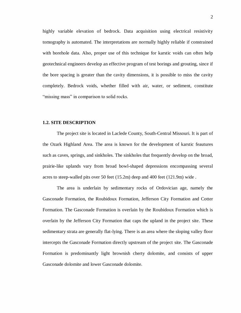
16

4. GEOPHYSICAL APPLICATION

Geophysical methods employ indirect, non-intrusive observations to characterize

and map variations in the physical properties of what lies concealed beneath the ground

surface. According to the Encycoledia of Caves and Karstic Science, 2004, “All

geophysical techniques require contrasts of some physical properties (density, electrical

resistivity, magnetic susceptibility and seismic velocity) between subsurface structures.

Although void space in rock may represent an enormous contrast in physical properties

that can be advantageous to an investigator seeking concealed caves, underground karst

openings are frequently small, irregular targets whose effects are easily masked by those

of surface irreglarities. In deep exploration, techniques that are useful usually are at the

expense of resolution and accuracy; conversely, techniques capable of generating high-

resolution images of shallow features are often based on high-frequency signals that are

rapidly attenuated as they propagate through deeper soil and rock”.

It is conventional in geotechnical engineering practice to obtain subsurface

information before embarking on any project. Mapping hidden karst is necessary when

engineering projects are planned in rock formations known to contain caves, because

karstic voids and collapses can compromise the integrity of building foundations, dams,

and bridges. Drilling of boreholes is one of the methods of obtaining subsurface

information. But if detailed subsurface information is needed, boreholes have to be

closely spaced in order to produce a reliable image of the subsurface. Unfortunately, such

drilling of multiple boreholes is time-consuming and uneconomical. More so, even

though the subsurface information obtained at boring location is very accurate, the

17

interpolation between boreholes can sometimes be erroneous due to significant variations

in karst terrain. Use of geophysical tools as a control reduces the number of required

boreholes and significantly decreases the ambiguity of the subsurface conditions.

4.1. GEOPHYSICAL TOOLS USED TO MAP VOIDS AND CAVES

Some of the common geophysical techniques that can be used to detect caves and

karstic voids are electrical resistivity, ground penetrating radar (GPR), gravity,

electromagnetic (EM), and seismic reflection. All these methods have their strengths and

weaknesses, so the choice of method to use depends on a number of factors such as the

size and depth of anticipated voids, reason for delineating voids, desired resolution of

voids, nature of background materials or bedrock surrounding the voids, type of materials

that may fill the voids (such as clay or water), depth to groundwater, size of the

investigation area and sources of cultural interference like power lines and fences in the

investigation area.

4.1.1. Ground Penetrating Radar (GPR) Method. In ground penetrating radar

(GPR) method, pulses of electromagnetic energy penetrate the ground and are partially or

totally reflected from rock or soil boundaries with contrasting electrical properties

(notably their dielectric constants, or permittivity). Air-filled voids and layers of water-

saturated sediment are strong radar reflectors. The reflected signals are detected on the

ground surface and are collated by computer to produce the ground profiles. But clay-rich

soils attenuate GPR signals and can restrict depth investigation to just 1foot (0.30m).

4.1.2. Gravity Method. In gravity method, the negative density contrast between

the target and the surrounding earth materials is identifiable as a local reduction in the

18

Earth’s gravitational acceleration (g) measured at the surface. Gravity surveys can

distinguish heavily karstified zones from nearby areas with a lower overall void space,

but gravity tells us little about the size and shape of individual voids. Also, interpretation

of gravity anomaly is limited by ambiguities; voids may still be present where no

anomaly is detected due to coincidental combination of additive and negative anomalies.

Another drawback is that gravity data needs a lot of corrections such as topography,

elevation, latitude and tidal corrections. All these have to be applied to the data before

they can be modeled.

4.1.3. Electromagnetic Method (EM). Electromagnetic method (EM) also uses

electromagnetic waves that are transmitted into the ground. Where the waves encounter

electrical conductors in the ground, they induce electrical currents in these conductors,

which in turn generate electromagnetic waves that can be collected at the surface by an

antenna. It can be useful in clay and water-filled voids. Its limitations are that air-filled

voids or fractures are transparent to electromagnetic signal and are difficult to detect.

Another major limitation of EM is ambiguity, because it may be difficult to isolate

changes in depth to bedrock from lateral changes in electrical conductivity.

4.1.4. Seismic Reflection Method. Seismic reflection surveys can detect voids

because the large negative reflection coefficient that exists between air and rock, or water

and rock, generates an echo that is strong and reverses the phase of the signal. Single sets

of ground-based seismic data have often failed to produce interpretable results, but

tomographic sections (imaging by sections or layers) have proved more useful. The major

limitation is that it demands expensive exploration infrastructure such as computer

analysis of large banks of data and incorporation of boreholes.

19

4.1.5. Electrical Resistivity Tomography Method. Electrical resistivity method

utilizes contrasting electrical properties to characterize and map buried rock. Electrical

current is transmitted directly into the ground through a pair of electrodes, which results

in a voltage change measured between a second pair of electrodes. The apparent

resistivity (ρa) of the ground can be calculated, and since low porosity bedrock usually

exhibits an electrical resistivity higher than overlying sediment, the buried topography

can be interpreted. Electrical resistivity can map lateral and vertical variations in apparent

resistivity of geologic material. It can approximate the size, shape and depth of air-filled

caves.

20

5. LITERATURE REVIEW: ELECTRICAL RESISTIVITY

TOMOGRAPHY (ERT)

Tomography means using any kind of penetrating wave for sectional imaging of a

structure or object, while the image produced is a tomogram. The method of using

electrical resistivity to partition the earth based on varying resistive properties of the earth

materials to produce a tomogram is called electrical resistivity tomography (ERT).

Electrical resistivity tomography (ERT) has proven to be an effective geotechnical

and environmental engineering tool. It is widely applied in determining the depth to

bedrock, locating of contaminated plumes, acquiring information on elevation of

groundwater table, etc. This method is especially preferred for site characterization in

karst terrains (Zhou, 1990). When electrical resistivity tomography is used in

combination with exploratory boreholes, the cost and time required for project execution

and completion can be significantly reduced. When the geophysical data are constrained

by borehole control, they can provide accurate and high resolution interpretations. Also,

the use of this geophysical method can be of immense help in terms of sitting additional

borehole control.

Electrical resistivity tomography technique has been successfully used in different

situations by numerous investigators (Anderson, et al., 2006; Hiltunen D. R. and Roth M.

J. S., 2008; Garman, K. M. and Purcell, S. F., 2008; Loke, M. H., 2008; Zhou, et al.,

2002; Zhou, et al., 2000; Hamzah, et al., 2006; Cardimona, S., 2008; Dong, et al., 2008)

to assess karst terrains.

Electrical resistivity tomography when compared with other geotechnical

investigation techniques such as trenching and borehole drilling proves to be rapid in

21

terms of data acquisition. It is also relatively inexpensive and less labor intensive. In karst

terrains where lateral variations in the depth to bedrock vary greatly, interpolation of the

subsurface conditions between two boreholes can often provide erroneous results. The

use of electrical resistivity tomography (ERT) can provide more precise information on

ground conditions between borehole locations. Also data can be obtained without

interrupting investigated objects or area (Non-Destructive Test).

Like most engineering and geophysical techniques, electrical resistivity

tomography (ERT) has its limitations and challenges. For example, if an area is covered

by concrete or asphalt, it is difficult to plant the metal stakes used to connect electrodes to

the ground for resistivity measurement to be taken. Also, vertical resolution of resistivity

data tends to decrease with depth.

The basic concepts of electrical resistivity technique used for this project are

described below.

5.1. CURRENT FLOW IN THE SUBSURFACE

Electrical current flow in the subsurface is primarily electrolytic. Electrolytic

conduction involves passage of charged particles by means of groundwater. Charged

particles move through liquids that infill the interconnected pores of permeable materials

(Robinson, 1988). When an electrical resistivity tomography survey is conducted in karst

terrain, current flow is generally assumed to be electrolytic rather than electronic.

22

5.2. RELATIONSHIP BETWEEN GEOLOGY AND RESISTIVITY

Variations in the resistivity of subsurface materials are mostly a function of

lithology. Information about resistivity variations within the subsurface can be associated

with different materials. Some resistivity values are given in Table 5.1.

Table 5.1.Resistivity of common Earth’s materials (Robinson, 1988)

Earth Material

Resistivity,

Average or Range

(Ohm-m)

Earth Material

Resistivity,

Average or Range

(Ohm-m)

Granite 102-10

6 Sandstone 1-10

8

Diorite 104-10

5 Limestone 50-10

7

Gabbro 103-10

6 Dolomite 10

2-10

4

Andesite 102-

104

Sand 1-103

Basalt 10-107

Clay 1-102

Peridotite 102-10

3 Brackish water 0.3-1

Air ˜ 0

Seawater 0.2

From Table 5.1, it can be noted that most materials are characterized by resistivity

values that vary by several orders of magnitude. For example, limestone has resistivity

values ranging from 50 ohm-m to 107 ohm-m. Most minerals are considered to be

insulators or resistive conductors. So in the majority of rocks, electrical current flow is

accomplished by passage of ions in pore fluids (electrolytic conduction). The

conductivity, which is the inverse of resistivity, is mostly affected by porosity, saturation,

salinity, lithology, clay content and to some degree by temperature. Accordingly,

materials with constant mineralogical composition can possess different resistivity

values, depending on all the above mentioned parameters.

23

5.3. OHM’S LAW AND RESISTIVITY

In 1872, George Simon Ohm derived empirical relationship between the

resistance (R) of a resistor in a simple series circuit, the current passing through the

resistor (I), and the corresponding change in potential (Δ V) :

Δ V = I R (5.1)

A simple series circuit that consists of a battery connected to a resistor by a wire

demonstrates this relationship (Figure 5.1). By using Ohm’s Law, the value of resistance

(R) can easily be calculated by plugging values of voltage (Δ V) and current (I) in the

equation (5.1). The last two values are given because they can be measured. The

electrical resistivity tomography concept is based on this relationship (Equation 5.1), with

the assumption that the resistor in the circuit (Figure 5.1) is the Earth.

There is another relationship that defines resistance (R) as a function of geometry

of a resistor and the resistivity of the cylindrical-shaped body:

R= ρL/A (5.2)

This equation shows that the magnitude of resistance is affected by the length (L)

and the cross-sectional area (A) (Figure 5.1) of the cylindrical-shaped body through

which electrical current flows (resistor). A factor that defines the ease with which

electrical current flows through the media is known as resistivity (ρ).

24

Figure 5.1.Electric circuit for illustration of Ohm’s Law

By rearranging equation (5.2), the resistivity can be expressed as:

ρ = R A/L (5.3)

The electrical resistivity of any material is the resistance between the opposite

faces of a unit cube of the material. Resistivity is an internal parameter of the material

through which current is compelled to flow and describes how easily this material can

transmit an electrical current. High values of resistivity imply that the material making up

the wire is very resistant to the flow of electricity. Low values of resistivity show that the

material making up the wire transmits electrical current very easily.

5.4. THEORETICAL DETERMINATION OF RESISTIVITY

The estimation of the apparent resistivity of the earth is relatively simple if

several assumptions are made.

The first assumption is that a model-Earth is uniform and homogeneous, thus it

possesses constant resistivity throughout the entire earth.

25

The second assumption is that the Earth is a hemispherical resistor in a simple

circuit consisting of a battery and two electrodes (the source and the sink electrodes)

pounded into the ground (Figure 5.2). The battery generates direct electrical current that

enters the Earth at the source electrode connected to the positive portal of the battery. The

current exists at the sink electrode coupled to the negative portal of the battery.

Figure 5.2.Current lines radiating from the source and converging on the sink electrodes

(Edwin S. Robinson, 1989)

When the current is introduced to the ground, it is compelled to move outward

from the source electrode. Due to the assumption that the earth is homogeneous, the

current spreads outward in all directions from the electrode, and at each moment of time,

the current front will move through a hemispherical zone. The area of such a

hemispherical zone can be found from the relationship:

26

A = 2πd2 (5.4)

Where d is the distance from the source electrode to the point on the hemispherical

surface defined by Equation (5.4), Figure 5.2.

By substituting equation (5.4) into equation (5.3), we can obtain an expression

that defines the resistance of the media at a point separated from the source by distance d:

R = ρ/ 2πd (5.5)

The potential difference resulting from the flow of current through the hemispherical

resistor can be found from combining Ohm’s law expressed by Equation (5.1) and

Equation (5.5):

V= ρ π = V0- Vd (5.6)

Where V0 is a potential at the source electrode and Vd is a potential at the surface of the

hemisphere with radius d.

This equation demonstrates that for any point located at the hemispherical surface

with radius d, the potential between this point and the source electrode is the same. Such

a hemisphere is a surface of constant potential and is called an equipotential surface. In

other words, the potential difference between a source and any point on the equipotential

surface has the same numerical value.

27

When the two electrodes are at a finite distance from each other, the potential at

any point M separated by distance d1 from the source electrode, and distance d2 from the

sink electrode, can be found as the sum of the potential contributions from source and

sink electrodes for point M (Figure 5.3).

Iρ/2π [1/d1 -1/d2] (5.7)

This equation can be employed to calculate the potential point by point

throughout the earth. By plotting these points and connecting those that are equal, the

equipotential surfaces can be obtained (Figure 5.3).

Figure 5.3.Current lines and equipotential surfaces in a medium of uniform resistivity

(Edwin S. Robinson, 1989)

28

5.5. APPARENT RESISTIVITY

To acquire 2-D electrical resistivity tomography data in the field, a four- electrode

array can be used. Two of these electrodes are used to inject electrical current into the

ground and are referred to as current electrodes (Figure 5.4; indicated by letters A and B),

and the other two electrodes are connected to a voltmeter and are used to measure the

potential difference between electrodes (Figure 5.4; shown by letters N and M).

Figure 5.4. Current electrodes A and B and potential electrodes M and N

Current flow direction is shown by red lines and equipotential surfaces are

indicated by blue lines. The assumption that the media through which the current is

compelled to flow is homogeneous provides for a constant value of resistivity irrespective

of where the voltmeter electrodes are placed.

29

Taking into account the geometry of the electrodes’ configuration, as illustrated in

Figure 5.4, the electric potential at point M can be deduced from the equation:

VM = Iρ/2π [1/d1 - 1/d2] (5.8)

VN = Iρ/2π [1/d3 - 1/d4] (5.9)

Therefore, the potential gradient between these two points, VMN, is

VMN = VM - VN = Iρ/2π [1/d1 - 1/d2-1/d3 + 1/d4] (5.10)

In practice, subsurface materials possess different physical characteristics, and the

assumption that resistivity is the same everywhere is not true. Thus, resistivity values that

are measured in the field are average resistivity values between two equipotential

surfaces, and are known as apparent resistivity values ρa. It can be expressed as:

ρ a = K * VMN/ I (5.11)

Where K is the geometric factor that depends on the electrode array configuration.

K = 2π/ [1/d1 - 1/d2-1/d3 + 1/d4] (5.12)

30

5.6. ELECTRICAL RESISTIVITY ARRAY CONFIGURATION

For modern electrical resistivity tomography surveys, multi-electrode systems are

preferred. The greater the number of electrodes permanently attached to multi-core cable,

the higher the investigation capabilities, and less time is spent in the field. Use of multi-

electrode system allows combination of vertical sounding and horizontal profiling data to

be collected simultaneously. Also it allows the generation of a two-dimensional model of

resistivity distribution (Lateral and Vertical).

For 2-D imaging using a modern multi-electrode system, the spacing between

electrodes stays fixed for the entire survey. Measurements are taken sequentially using

different sets of four electrodes controlled by switching device. The depth of

investigation is a function of the array type, the length of array and the physical

parameters of material underlying the area of interest, and typically ranges from one-third

to one- fifth of the length of the entire array (Robinson et al., 1988).

5.7. 2-D RESISTIVITY ARRAYS

Some of the more common electrode configurations such as Wenner array,

Schlumberger array, and Dipole-dipole array are briefly discussed below. The geometry

of an electrode array depends on the target depth, the time allowable for data acquisition,

and the required spatial resolution.

When a multi-electrode system is used, the spacing between all electrodes

remains the same, while the distance between current and potential electrodes depends on

electrode configuration. This distance is controlled automatically by resistivity meter.

31

Most electrical resistivity tomography surveying is done with one of the electrode

geometries illustrated in Figure 5.5.

For the 2-D Wenner Array (Figure 5.5), current and potential electrodes are

separated by equal distance ‘a’ such that,

AM = MN = NB = a (5.13)

All the electrodes are arranged along a continuous line, also known as survey line

or traverse. The geometric factor for Wenner Array can be expressed as,

KW = 2 * π * a (5.14)

Figure 5.5. The most common electrode array configurations

(http://pangea.stanford.edu/research/groups/sfmf/docs/DCResistivity.pdf).

32

Figure 5.5. Cont’d. The most common electrode array configurations

For the 2-D Schlumberger array (Figure 5.5), the current electrodes A and B are

located on the opposite sides from center point of the array .The passive electrodes N and

M are placed between A and B electrodes.

Suppose the current electrodes A and B are separated by distance ‘L ‘, and the

passive electrodes N and M are separated from the center by distance ‘b’, the geometric

factor for Schlumberger array can be given by the expression:

KS = π (L2 - b

2 ) /2b (5.15)

The third geometry is attributed to the Dipole - dipole configuration, where the potential

electrodes M and N are not placed between the current electrodes A and B (Figure 5.5).

33

The Dipole - dipole array is logistically the most convenient array used in the field,

especially for large scale projects. In this type of array, all four electrodes are placed

along the same line, and the distance between the current electrodes A and B is equal to

the distance between the potential electrodes M and N, represented by ‘a’, given by the

following,

AB = MN = a (5.16)

The distance between the middle points of current and the passive electrode sets is

an integer multiple of a, and the factor itself is assigned to be equal to n (Figure 5.5).

The geometric factor K can be found from the following expression:

K DD = π *n (n2 -1)*a (5.17)

The dipole-dipole method was used in this project because this type of array has proven

to be the most efficient in areas with great lateral variations in depth to bedrock (Zhou,

2000).

34

6. DATA ACQUISITION

The geophysical investigation was conducted towards the end of February 2011,

when the average temperature was about 30 degrees F. The initial plan for the project was

to run six electrical resistivity profiles; four would be parallel to the bridge pier in

question and two traverses would be roughly perpendicular or at a skewed angle on either

side of the bridge bent. The parallel profiles would be one on either side of the bridge

pier. The first profile acquired was profile 1(Figure 6.1), and was close to profile 2

(Figure 6.2). Profile 5 (Figure 6.3) was roughly perpendicular to other profiles.

Figure 6.1. Data acquisition of profile 1

35



36

But after acquiring the fifth resistivity data set (profile 5), the equipment

developed a fault, and the sixth data set (profile 6) could not be acquired. Profiles 5 and 6

were supposed to be the perpendicular profiles, so data interpretation was based on five

profiles (profiles 1-5) as shown in Figure 6.4.

The site plan (Figure 6.5) shows the location of all the boreholes and resistivity

profiles with respect to the bridge piers. Bridge pier 6 (C6) is the primary exploration

target.

5

1

2

Bridge Pier Θ Θ Voids

3

4

5

Figure 6.4. Sketch of electrical resistivity traverses at project site

37

Figure 6.5. General site plan

Locations of fourteen boreholes drilled at the site are shown as green dots, C

represents the bridge pier. Bridge pier C6 is the primary exploration target. Boreholes

SW-1, BW-1, BW-2, BW-3 and BW- 3A are not logged. Boreholes T-11-03 to T-11-10

are logged boreholes. The five resistivity profiles are represented by T1, T2, T3, T4 and

T5.

The electrical resistivity profiles were acquired using a SuperSting R8 resistivity

unit with 72 electrodes spaced at 2.5 feet (0.76m) each for a total traverse length of about

177.5 feet (54.1m). The profiles were separated from one another by 4.5 feet (1.4m)

C6

C1

C2

C3

T-11-07

T-11-03 T-11-05

T-11-10

BW-1

BW-2

BW-3A

BW-3

T-11-08

SW-1

T-11-04

T-11-09

T-11-06

T-11-06R

38

except profiles 2 and 3 which had a separation distance of about 7.5 feet (2.3m) due to

presence of the bridge pier.

The SuperSting R8 resistivity unit makes use of dipole-dipole array

configuration. This type of configuration is very sensitive to horizontal changes in

resistivity (Zhou, 2007), which means that it performs well in mapping vertical structures

such as vertically oriented solution-widened joints. A small electrode interval of 2.5 feet

(0.76m) was chosen to ensure high resolution at the required depth of investigation. Each

profile length was approximately 177.5 feet (54.1m) long and the profiles were separated

from one another by 6 feet (1.82m) interval except profile 2 and 3 with separation

distance of about 10.7 feet (3.26m) due to obstacle.

6.1. EQUIPMENT USED FOR ERT

Electrical resistivity tomography (ERT) involves introduction of electrical current

into the subsurface by means of electrodes attached to the ground. All required

measurements are by resistivity meter. For this project, a multi-channel portable memory

Earth resistivity meter-SuperSting R8/IP, manufactured by Advanced Geosciences, Inc.,

(Figure 6.6) was used. The SuperSting was powered by a 12-volt battery. For larger scale

projects, two batteries can be used.

39

Figure 6.6. Earth resistivity meter-SuperSting R8/IP, manufactured by Advanced

Geosciences Inc.

For this project, seventy two (72) electrodes were connected to the insulated low

resistance multi-core cable. Each electrode is tied to a metal stake pounded on the ground

using a rubber - band, this allows electric current to flow from the electrode to the ground

or subsurface. The electrodes are connected to the switching unit which also connects the

SuperSting. Laptop computer is connected to the SuperSting, and the whole set up is

powered by a 12- volt battery. Dipole - dipole array configuration was used.

In dipole - dipole array configuration, as shown in Figure 6.7, the electrodes are

attached to a multi-core cable in a straight line.

Figure 6.7. Electrical resistivity dipole-dipole array configuration used in the field

40

The cable is connected to the switching unit hardwired into the SuperSting

resistivity meter. The unit controls the selection of the current (A&B) and potential

(M&N) electrodes for each measurement. The SuperSting resistivity meter is connected

to a laptop computer where the data is stored.

6.2. ELECTRICAL RESISTIVITY TOMOGRAPHY DATA PROCESSING

The resistivity data sets collected in the field were converted into resistivity

models for interpretation of subsurface conditions using the RES2DINV software.

ERT data was processed using the following steps;

Inspection of the resistivity data sets for presence of unreasonably high and low

(negative) resistivity values called “ bad data points” (Loke, 2004).

Removal of “bad data points”.

Compilation of a resistivity model/ERT resistivity profile that displays horizontal

and vertical resistivity distribution.

Before processing, the data acquired had to be inspected for presence of “bad data

points” (Loke, 2004). “Bad data points” mean resistivities of unrealistically high or low

(negative) values. “Bad data points” can be caused by several factors, such as failure

during survey of equipment used, for example electrode malfunction. Also, very poor

electrode - ground contact can result to “bad data points”. In addition, when a metal stake

attached to an electrode is driven into an ice lens, resistivity measurements are affected.

Ice acts as an insulator, and affects resistivity measurements. This is a problem for

surveys done in winter.

41

Inspection of “bad data points” is done by viewing a profile plot, illustrated in

Figure 6.8. The “bad data points” appear as stand out points. All “bad data points” are

marked as red plus signs. The RES2DINV software offers an option that allows for

removal of such points manually by simply clicking on them. After the resistivity data

sets acquired in the field were inspected and all unrealistic values removed, the

RES2DINV software used an inversion algorithm to convert the measured resistivity

model/ERT resistivity profiles to a geologic model which reflect lateral and vertical

resistivity distribution.

Figure 6.8. Example of a data set with a few bad data points (Loke, 2004)

The software creates a resistivity model/resistivity profile that has the same

resistivity distribution as the actual resistivity distribution below the corresponding

traverse. To increase the quality of the calculated model, the Root Mean Square (RMS)

42

method is used, (Loke, 2004). In this method, the smaller the RMS value, the better the

calculated model correlates with real resistivity distribution. In this project, an RMS

value of 50% was used.

To create a resistivity model, the RES2DINV subdivides the subsurface into a

finite number of rectangular pixels. Each pixel is assigned a resistivity value which

represents the resistivity of different materials encompassed within that discrete pixel;

therefore some lateral and vertical smoothing takes place (Anderson, 2006).

The size of the pixels is affected by the spacing between the adjacent electrodes.

Horizontal dimension of a pixel is equal to lateral distance between adjacent electrodes,

and at shallow depth, the vertical dimension is approximately equal to 20% of the spacing

between two adjacent electrodes. With increasing depth of investigation, the vertical

dimension of pixels gradually increases up to 100% of the distance between adjacent

electrodes (Anderson et al., 2006). The resolution of the output model is a function of the

pixel size (Figure 6.9). Thus, with increasing depth of investigation, resolution decreases.

Figure 6.9. Arrangement of the blocks used in a model together with the data points

43

When a Dipole-dipole array is used, the maximum depth of investigation is

approximately 20%-25% of the array length but this is affected by subsurface condition

such as the top layer of the ground being very dry. For this project, the depth of

investigation was about 36 ft (11m).

The ERT resistivity profiles generated (Figure 6.10 - Figure 6.14) are later

interpreted by picking the inverse model resistivity sections.

Caption A (Figure 6.10) is the measured apparent resistivity pseudosection which

represents the data set acquired in the field, caption B is the calculated apparent

resistivity pseudosection which represents a synthetic model that is used to estimate the

size of the pixels at different layers and C represents the Inverse model resistivity section

which represents the true geologic model of the subsurface. The unit electrode spacing

was 2.5 feet (0.76m).

Figure 6.10. Unedited/raw profile 1

A

B

C

44






was 2.5 feet (0.76m).






A

B

C

45


was 2.5 feet (0.76m).







was 2.5 feet (0.76m).

A

B

C

46







was 2.5 feet (0.76m).

A

B

C

47


6.3. RESOLUTION LIMITATION OF ERT METHOD

Resolution is a function of electrode spacing and resistivity contrast between

lithologically different earth materials. The resolution of electrical resistivity tomography

(ERT) profile defines the accuracy of interpretation of subsurface conditions. The size of

a pixel is a main estimate of ERT imaging resolution. In this thesis, at shallow depth, the

width of the pixel is about 2.5ft (0.76m) and the vertical dimension of the pixel is around

0.5ft (0.15m). This means that at this shallow depth, all objects that are less than the size

of the pixel will be easily detected. With increasing depth, the vertical dimension of the

pixels becomes greater and that reduces ERT resolution. To estimate the size of all

detectable objects at a certain depth, it is recommended to compile a synthetic resistivity

model. The model can be used to visually estimate the size of the pixels at different depth

A

B

C

48

layers. During ERT survey, when current is induced to flow through deeper layers, the

distance between current and potential electrodes is gradually increased. This affects the

sensitivity of the ERT method. Gradually increasing the distance between electrodes

lowers the intensity of current flow, and accordingly the sensitivity of ERT survey. Thus,

interpretation of smaller scale objects at greater depths becomes increasingly difficult and

sometimes small objects can be missed or misinterpreted.

Resistivity contrast is another parameter that defines the resolution of ERT

profile. When lithologically different materials exhibit similar conductivity parameters,

sometimes it is difficult to differentiate them simply on the basis of their resistivity

parameters. For example, both intact bedrock and air-filled voids typically are

characterized by high resistivity values. When an air-filled void is embedded in intact

limestone, it typically cannot be easily detected on resistivity profile because of low

resistivity contrast. In the project site, there are some areas where resistivity

measurements were not acquired due to lack of resistivity contrast between the soils and

fractured bedrock. Resistivity contrast plays a major role in ERT method, but in a

situation where there is no signal due to close resistivity properties between earth

materials; borehole information can be used to complement resistivity data.

49

7. DATA INTERPRETATION

Because of variability in resistivities of earth materials, interpretation of electrical

resistivity tomography (ERT) data must be handled with caution. Factors such as

temperature, porosity, conductivity, salinity, clay content, saturation and lithology

generally affect the resistivity of earth materials. There are also overlaps of the resistivity

values of earth materials which in most cases are given as ranges of values rather than

absolute values. For example sandstone, limestone, dolomite, sand, and clay have

resistivity values that can range from 1 ohm-m to 108 ohm-m. For more effective data

interpretation, resistivity control for the lithologic materials in the study area would help

to reduce any ambiguity.

The objective of this survey was to map the lateral and vertical extent of water-

filled vugs near the unnamed bridge foundation at the project site, and possibly locate the

top of bedrock in that vicinity. With this, it would be possible to design an appropriate

engineering solution such to strengthen the load-bearing capacity of the bridge

foundation.

The ERT resistivity profile and model were used for interpretation of subsurface

conditions within the study site. This ERT survey was complemented by geotechnical

ground sampling obtained from borings. Nine boreholes, designated T-11-03 through T-

11-11 were drilled more-or-less along the resistivity traverses for site characterization.

The soil encountered in the borings consisted of lean clay and silty alluvium with varying

amounts of sand and gravel. The rock encountered on site was typically dolomite of

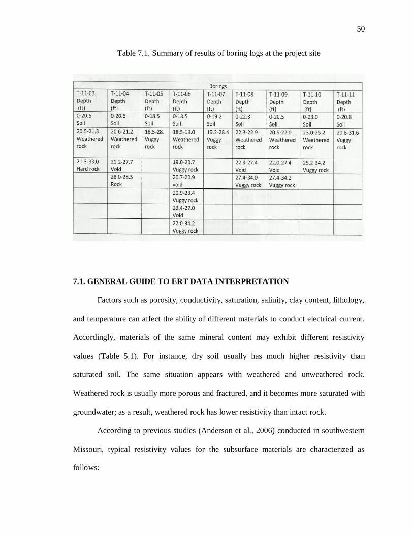
varying degrees of vuggyness and weathering. These results are summarized in Table 7.1.

50

Table 7.1. Summary of results of boring logs at the project site

7.1. GENERAL GUIDE TO ERT DATA INTERPRETATION

Factors such as porosity, conductivity, saturation, salinity, clay content, lithology,

and temperature can affect the ability of different materials to conduct electrical current.

Accordingly, materials of the same mineral content may exhibit different resistivity

values (Table 5.1). For instance, dry soil usually has much higher resistivity than

saturated soil. The same situation appears with weathered and unweathered rock.

Weathered rock is usually more porous and fractured, and it becomes more saturated with

groundwater; as a result, weathered rock has lower resistivity than intact rock.

According to previous studies (Anderson et al., 2006) conducted in southwestern

Missouri, typical resistivity values for the subsurface materials are characterized as

follows:

51

Moist clays in southwestern Missouri are normally characterized by low

resistivity values (usually less than 100 ohm-m) and may vary due to different

degrees of saturation, porosity, and layer thicknesses.

Moist soils and intensively fractured rocks intermixed with clay typically have

resistivity values between 100 and 400 ohm-m. Such variation is explained by

different porosity, saturation, clay content, and layer thicknesses.

Relatively intact limestone with minimal clay content is characterized by higher

resistivity values, typically more than 400 ohm-m. Resistivity values of intact

limestone may vary due to varying layer thickness, moisture content, porosity,

saturation, and impurities.

Air-filled cavities usually show very high resistivity values, usually more than

1000 ohm-m, but again, are variable depending on the conductivity of the

surrounding strata and depth/size/shape of void. Zones where relatively intact

bedrock is surrounded by moist loose materials (such as clay), or zones where air-

filled voids are embedded in relatively intact limestone, are zones of electrical

resistivity contrast. These zones can be successfully detected by electrical

resistivity tools.

The following explanations are necessary in ERT data interpretation.

The apparent resistivity is a term used for the field measurement, since without

interpretation; the resistivity measurement does not refer to any particular geologic

layer. The resistivity pseudosection produced consists of the measured apparent

resistivity pseudosection, the calculated apparent resistivity pseudosection and the

inverse model resistivity section. In this case, they are referred to as raw or unedited

52

profiles. In order to interpret a profile, say profile 1; the profile has to be edited. In

that case, the inverse resistivity model is picked and interpreted because it represents

the actual geologic model of the subsurface; which gives information on the vertical

distribution of layer thicknesses, depths and resistivities (Figure 7.1-Figure 7.5).

Figure 7.1. Interpreted profile 1

The black line indicates the interpreted top of bedrock; the resistivity value is less

than 400 ohm-m, this is based on studies conducted in southwestern Missouri (Anderson

et al., 2006) which showed that intensively fractured rocks intermixed with clay are

typically of resistivity values between 100 and 400 ohm-m. The rock is also highly

saturated. This is consistent with borehole control, where borehole T-11-07 was drilled

along traverse 1. The blue color with resistivity value less than 10 ohm-m appears to

represent a sediment/clay-filled vug , this is based on studies conducted in southwestern

53

Missouri where moist clays are normally characterized by low resistivity values usually

less than 100 ohm-m. The result shows that bedrock dips steeply from east to west.


The superposed black line indicates the interpreted top of bedrock, the resistivity

value is less than 400 ohm-m, this is based on studies conducted in southwestern

Missouri (Anderson et al., 2006) which showed that intensively fractured rocks

intermixed with clay typically have resistivity values between 100 and 400 ohm-m.

Resistivity value of about 110 ohm-m was recorded. The rock is also highly saturated;

this is consistent with borehole control T-11-05. The blue spots appear to be

sediment/clay-filled vugs with resistivity values less than10 ohm-m, this is based on

studies conducted in southwestern Missouri (Anderson et al., 2006) where moist clays are

normally characterized by low resistivity values usually less than 100 ohm-m. Bedrock

dips from east to west.

54

Figure7.3. Interpreted profile 3

The bridge pier, C6 is the primary exploration target, as such; four boreholes (B5,

B6, B8, and B9) which are designated as T-11-05, T-11-06, T-11-08 and T-11-09 in

boring table (Table 7.1) were drilled along traverse 3. The superposed black line indicates

the interpreted top of bedrock, a resistivity value of around 110 ohm-m was recorded,

indicating that the top of the bedrock is highly fractured; this is based on studies

conducted in southwestern Missouri (Anderson et al., 2006) which showed that

intensively fractured rocks intermixed with clay typically have resistivity values between

100 and 400 ohm-m. The bedrock here appears to be competent bedrock, with resistivity

value more than 1000 ohm-m. Void was encountered on this profile, and according to

studies in southwestern Missouri (Anderson et al., 2006), air-filled cavities usually show

very high resistivity values, usually more than 1000 ohm-m, but again, are variable,

depending on the conductivity of the surrounding strata and depth/size/shape of void.

55

The high resistivity value could also be as a result of the grout placed below the footing

years ago. Voids were encountered in boreholes B6, B8 and B9; this is consistent with

borehole control. The blue spots appear to be sediment/clay-filled vugs with resistivity

values less than10 ohm-m. This is based on studies conducted in southwestern Missouri

where moist clays are normally characterized by low resistivity values usually less than

100 ohm-m (Anderson et al., 2006).


The superposed black line indicates the interpreted top of bedrock .Void was

encountered on this traverse; this is consistent with borehole control where B4, B8 and

B9 designated as T-11-04, T-11-08 and T-11-09 in the boring log encountered voids

(Table7.1). Sediment/clay-filled vugs were few and small in sizes, with resistivity values

56

less than10 ohm-m. A high resistivity value above 3700 ohm-m observed, appears to be

gravel.


In this profile, T1, T2, T3 and T4 are positions of ERT profiles 1, 2, 3 and 4 with

respect to profile 5, and C3 is the position of bridge pier 3. This profile is orthogonal in

direction with the rest of the traverses; no borehole was drilled along this traverse as at

the time of this project. The black line indicates the top of bedrock with resistivity value

of about 110 0hm-m, this is based on studies conducted in southwestern Missouri

(Anderson et al., 2006) which showed that intensively fractured rocks intermixed with

clay typically have resistivity values between 100 and 400 ohm-m. Sediment/clay-filled

vugs are few and small in sizes with resistivity values less than10 ohm-m. High

resistivity value above 3700 ohm-m observed, appears to be saturated gravel used as

embankment fill.

57

Geophysical data, along with boring information was used to interpret the

subsurface conditions; consequently, the following conclusions were made:

Bedrock beneath the bridge pier is generally characterized by resistivity values of

less than 400 ohm-m, except on ERT profile 3 in immediate proximity to the

columns, where resistivity value up to 1000 ohm-m was observed. This relatively

low resistivity of bedrock is an indication that this rock is extensively fractured

and saturated.

Top of bedrock in proximity to the pier is interpreted as being at a shallow depth

to the east of the structure (based on ERT profile1) and at depths on the order of

20 feet (6m) immediately to the west of the structure . This indicates that bedrock

dips steeply from east to west beneath the pier.

The top of bedrock cannot be mapped with confidence on all the ERT profiles due

to the fact that interpreted fractured rock, in most places, is characterized by

resistivity values that are the same as the overlying soil. In places where they are

mapped, the top of bedrock is at a depth of around 20 feet (6m); this is consistent

with borehole control (Table 7.1).

At the eastern side of the pier, bedrock beneath the pier is generally characterized

by resistivity values of between 400 and 4000 ohm-m, and is interpreted as

competent rock except where shallow gravels appear to be present.

58

7.2. ENGINEERING SOLUTION APPLIED

Compaction grouting was the engineering solution employed to seal the voids,

and was based on the result of ERT and boreholes drilled at the project site (Table 7.2).

Table 7.2. Summary of sizes of voids and volume of grout used to seal the voids

Borehole Total depth

(ft.)

Range of voids

(ft.)

Vertical extent

(ft.)

Volume of grout placed

(cu.ft.)

T-11-04 28.5 21.2-27.7 6.5 378

T-11-06 34.2 20.7-27.0 3.8 410.4

T-11-08 34.0 22.9-27.4 4.5 506.2

T-11-09 34.2 22.0-27.4 5.4 492.7

BW-1 34.2 Not logged Not logged 26.9

BW-2 29.2 Not logged Not logged 13.5

BW-3 N/A Not logged Not logged Drilling aborted

BW-3a 25.0 Not logged Not logged 378.0

SW-1 27.5 Not logged Not logged 6.7

Total Volume of grout used: 2212.4 cubic feet = 81.94 cubic yards.

59

Based on the result of the borings and ERT, voids were detected in nine boreholes

drilled along resistivity traverses close to the bridge pier in question (C6) as shown in

Table 7.2. The voids were grouted using compaction grouting technique. Compaction

grouting, also known as low mobility grouting is a grouting technique that displaces and

densifies loose granular soils, reinforces fine grained soils and stabilizes subsurface voids

or sinkholes. This is usually done by injecting low-slump, low-mobility aggregate grout

using an injection pipe. From the result of the grouting program, a total volume of about

2212.4 cubic feet (81.94 cubic yards) of grout was used to seal the voids and stabilize the

ground around the structure.

The result of the interpretation of the five ERT profiles acquired showed a linear

topographic feature (Figure 7.6) that is believed to reflect groundwater flow direction.

Groundwater is continually moving, often very slowly. The movement is controlled by

gravity, topography and geology. Gravity is the major driving force and thus groundwater

is always moving from areas of higher elevation to lower elevation. The project site has

an undulating topography which controls groundwater movement. Another important

factor that controls groundwater movement in this area is the nature of rock formations

that are found in the area. Rock formations in the area are predominantly dolomite

(Gasconade dolomite) which dissolves in slightly acidic waters; the dissolved materials,

along with the remaining insoluble parts of the rock are transported from the site through

solution enlarged openings in the bedrock. Also, the top of bedrock in the project site is

highly fractured, so fracture is also a factor in groundwater flow direction in the site.

60

Figure 7.6. Lineament showing horizontal bedding plane

The interpretation is consistent with borehole data which shows that voids occur

approximately at the same depth of around 22 feet (6.7m). This lineament as (Figure 7.6)

is an indication that solution cavities encountered beneath the bridge developed most

probably along horizontal bedding planes rather than vertical bedrock joints.

61

8. CONCLUSION

A structural support was needed to strengthen the load-bearing capacity of a

bridge foundation in Laclede County in South-Central Missouri due to increasing volume

of traffic and age of the bridge (constructed in 1955). During the construction of a drilled

shaft for the substructure a few feet north of the north footing of the pier, voids were

noted beneath a roughly 2 - foot (0.6m) - thick cap of dolomite rock near the bridge.

Water - filled voids were also observed very close to the bridge pier. Because of these,

there were concerns about the integrity of the rock beneath the existing bridge

foundation, and had to be mapped to determine the extent of the voids.

In order to map the lateral and vertical extent of the voids, as well as locate the

top of bedrock near the bridge foundation, electrical resistivity tomography (ERT) was

deemed the appropriate geophysical tool to be used for site characterization,

complemented by borehole information (borehole control). The result of this survey was

used to determine the proper engineering solution to be employed to achieve this purpose.

According to the results obtained, the following conclusions were made:

Solution cavities encountered beneath the bridge are limited in size and extent.

They developed most probably along horizontal bedding planes rather than

vertical bedrock joints, and are likely to be partially clay-filled.

The ERT survey did not show any room-sized void, showing that the voids are

limited in size and extent based on the volume of grout used (2212.4 cubic

feet/81.94 cubic yards) to seal the voids.

62

The voids present on site appear to be filled with dirty water and as such exhibit

resistive properties very close to the surrounding vuggy rock.

Choosing the appropriate geophysical method and constraining it with ground

truth from borings will enhance site characterization for geotechnical practice. The choice

of method to use depends on a number of factors such as the size and depth of anticipated

voids, reason for delineating voids, desired resolution of voids, nature of background

materials or bedrock surrounding the voids, type of materials that may fill the voids (such

as clay or water), depth to groundwater, size of the investigation area and sources of

cultural interference in the investigation area. In some cases, different electrode

configurations used in electrical resistivity tomography (ERT) method show similar

results especially in a site that is uniform, though each configuration has advantages and

disadvantages depending on the physical properties of the host environment and the

desired target. Cultural interference in this context refers to power lines and fences which

affects resistivity measurements when present at project site. Because power lines and

fences are conductive, and conductivity is an inverse of resistivity, these materials lower

the resistivity of earth materials in the investigation area, thereby giving inaccurate

resistivity measurements.

63

BIBLIOGRAPHY

Advanced Geosciences, Inc., “Instruction Manual for the SuperSting with Swift

Automatic Resistivity and IP System,” 2011.http://www.agiusa.com.

Aley, Thomas J., Williams, James H., Massello and James W., “Groundwater

Contamination and Sinkhole Collapse Induced by Leaky Impoundments in

Soluble Rock Terrain,” Missouri Geological Survey and water Resources,

Engineering Geology Report; Number 5, 1972.

Edwin S. Robinson, “Current lines Radiating from the Source Electrode and Converging

on the Sink Electrode,” Field Geophysics, Open University Press and Halsted

press Inc., 1989.

Encyclopedia of Caves and Karst Science, “Geophysical Detection of Caves and Karstic

Voids,” ISBN: 0-203-48385-5, January 2004.

Geotomo Software Malaysia, “Geoelectrical Imaging 2D & 3D, RES2DINV, Ver 3.56,”

2011. www.geoelectrical.com.

Haobin Dong, Chuanlei Wang, Huaping Wang, Xinhui Cai and C. Richard Liu, “Two-

Dimensional Resistivity Imaging Survey for Detecting Termitaria in a Dam”

2011.http://ieeexplore.ieee.org/stamp/stamp.jsp?tp=&arnumber=1673257&userT

ype=inst.

Hiltunen, D. R., and Roth, M. J. S., “Investigation of Bridge Foundation Sites in

Karst Terrains via Multi –Electrode Electrical Resistivity,” 2011.

http://www.dot.state.fl.us/statematerialsoffice/geotechnical/conference/materials/h

iltunen-roth.pdf.

James A. Martin, Robert D. Knight and William C. Hayes “The Stratigraphic

Succession in Missouri; Ordovician System,” Missouri Geological Survey and

Water resources, 1961.

James E. Vandike, “Geologic and Stratigraphic Units in Laclede County,” Missouri

Geological Survey and Water Resources, 1993.

James W.Duley, John W.Whitfield, Ardel W.Rueff and James E.Vandike,

“Geologic and Hydrologic Resources of Laclede County, Missouri, open file

Report,” 1992.

http://www.geoelectrical.com/

http://ieeexplore.ieee.org/stamp/stamp.jsp?tp=&arnumber=1673257&userType=inst

http://ieeexplore.ieee.org/stamp/stamp.jsp?tp=&arnumber=1673257&userType=inst

64

K. Michael Garman and Scott Purcell, “Three-Dimensional Electrical Resistivity

Surveys to Identify Buried Karst Features Affecting Road projects,” 2011.

http://www.dot.state.fl.us/statematerialsoffice/geotechnical/conference/materials/g

arman-purcell.pdf.

Karst Map of the US, Published by AGI, http://www.caves.org/pub/journal/pdf/V64/

V64n1-Veni.pdf. 2011.

Loke, M. H., “Electrical Imaging Surveys for Environmental and Engineering Studies,”

2011. http://www.terraip.co.jp/lokenote.pdf, Pp 445-478.

Neil L. Anderson, Derek B.Apel and Ahmed Ismail “Assessment of Karst Activity

At Highway Construction Sites Using the Electrical Resistivity Method,”

unpublished report for MoDOT, 2006.

P.J. Gibson, P. Lyle, and D.M.George, “Application of Resistivity and Magnetometry

Geophysical Techniques for near-surface Investigation in Karstic Terrains in

Ireland,”Journal of Cave and Karstic Studies; Volume 39, August 2004; pp 35-38.

Steve Cardimona, “Electrical Resistivity Technique for Subsurface Investigation,” 2011.

http://citeseerx.ist.psu.edu/viewdoc/download?doi=10.1.1.135.2978&rep=rep.

Taylor and Francis, “Geophysical Detection of Caves and Karstic Voids,”

Encyclopedia of Caves and Karst Science, 2011.

Umar Hamzah, Rahman Yaacup, Abdul Rahim Samsudin, Mohd Shahid Ayub

“Electrical Resistivity Imaging of the Groundwater Aquifer at Banting, Selangor,

Malaysia,” Journal of Environmental Geology; Volume 49, Number 8/April,

2006; pp1156-1162.

Wallace B. Howe and John Koenig, “The Stratigraphic Succession in Missouri,” Volume

XL, Second Series, Missouri Geological Survey and Water Resources, 1961.

Wanfang Zhou, Barry F. Beck and Angela L. Adams, “Effective Electrode Array in

Mapping Karst Hazards in Electrical Resistivity Tomography,” Journal of

Environmental Geology; Volume 32, Number 8/ November, 2002; pp 922-928.

W. Zhou, B. F. Beck, and J.B. Stevenson, “Reliability of Dipole-Dipole electrical

Resistivity Tomography for Defining Depth to Bedrock in Covered Karst

Terrains,” Journal of Environmental Geology; Volume 39, Number 7/May, 2000;

pp 760-766.

http://www.dot.state.fl.us/statematerialsoffice/geotechnical/conference/materials/garman-purcell.pdf

http://www.dot.state.fl.us/statematerialsoffice/geotechnical/conference/materials/garman-purcell.pdf

http://www.caves/

http://www.terraip.co.jp/lokenote.pdf

http://citeseerx.ist.psu.edu/viewdoc/download?doi=10.1.1.135.2978&rep=rep

65

VITA

Jeremiah Chukwunonso Obi was born in Ogidi, Anambra State, Nigeria. He

received his Bachelors degree (BSc.hons.) in Geological Sciences in 1997 from Nnamdi

Azikiwe University Awka, Nigeria. He moved to the United States in 2008, worked for

some time and got admission into Missouri University of Science and Technology where

he received his Masters degree (M.S.) in Geological Engineering in May 2012.

The use of electrical resistivity tomography (ERT) to ...

Documents