The Use of AVHRR Thermal Infrared Imagery to Determine …pubs.aina.ucalgary.ca/arctic/Arctic44-S-130.pdf · to Determine Sea Ice Thickness within the Chukchi Polynya ... Polynyas

VOL. 4 4 , SUPP. 1 (1991) P. 130-139 ARCTIC

The Use of AVHRR Thermal Infrared Imagery to Determine Sea Ice Thickness within the Chukchi Polynya

J.E. GROVES’ and W.J. STRINGER’

(Received 4 October 1990; accepted in revised form 29 July 1991)

ABSTRACT. Sea ice thickness changes over a nine-day period are determined for the Chukchi Polynya using Maykut’s (1986) and Kuhn et al.’s (1975) theoretical predictive models. The models relate ice thickness to sea ice surface temperature., air temperature, wind speed, and sea water temperature. Sea ice surface temperatures are derived from AVHRR imagery and meteorological observations are taken from the synoptic weather station at Barrow, Alaska. The Maykut equation yields results that appear to be realistic for the ice thickness distribution within the polynya at the beginning stages of polynya formation. Ice thickness calculations at the later stages of polynya formation are partially invalidated by the movement of large floes to the oldest part of the polynya in response to a wind from the northeast. Such a major disturbance on the surface of the polynya com- plicates the identification of the type and thickness of ice that is forming. These results offer encouragement for the prospects of future field studies to validate and refine the technique and for the extension of the technique to calculation of heat transfer and salt rejection within the Chukchi Polynya and other polynyas. Key words: polynya, Chukchi Sea, ice thickness, AVHRR imagery, surface heat transfer, ice growth

RÉSUMB. On a déterminé les changements dans I’épaisseur de la glace sur une #riode de neuf jours dans la polynia de la mer des Tchouktches, en utilisant les modbles de prédiction théoriques de Maykut (1986) et de Kuhn et al. (1975). Ces modbles établissent une relation entre d’une part I’épaisseur de la glace et d’autre part sa temp6rature de surface, la temp6rature de l’air, la vitesse du vent et la temp6rature de l’eau de mer. Les tem- pératures de la surface de l’eau de mer sont tirées des images prises au radiombtre perfectionné B trbs haute résolution, et les observations météorologiques proviennent de la station de météorologie synoptique de Barrow en Alaska. L’Cquation de Maykut donne des r6sultats qui semblent réalistes pour la distribution de I’épaisseur de la glace dans la polynia, aux stades initiaux de sa formation. Les calculs de I’épaisseur de la glace durant les stades ultérieurs de formation de la polynia deviennent en partie non valides B cause du mouvement de grands glaçons flottants vers la partie la plus ancienne de la polynia, mouvement dû B un vent du nord-est. Une perturbation de ce genre & la surface de la polynia complique I’identification du type de glace en formation et de son épaisseur. Ces résultats offrent un encouragement pour de futures études éventuelles sur le terrain en vue de valider et de perfectionner cette technique ainsi que de l’étendre au calcul du transfert thermique et du rejet salin dans la polynia de la mer des Tchouktches et d’autres polynias. Mots clés: polynia, mer des Tchouktches, épaisseur de la glace, images prises au radar perfectionné B trbs haute résolution, transfert thermique de surface, croissance de la glace

~.

Traduit pour le journal par Nésida Loyer.

INTRODUCTION

Polynyas are mesoscale areas of open water or thin ice in sea ice covered regions. Stringer and Groves (1991) find that at maximum from 2 to 5% of the surface normally covered by ice in the Bering and Chukchi seas is present as open water within coastal polynyas. Participants in the International Arctic Polynya Program (IAP2, 1989) state that open water in polynyas represents 3-4% of the surface area of the Arctic. Polynyas are responsible for u to 50% of its oceanic and atmospheric heat transfer (IAP , 1989). This transfer takes place at the surface of thin ice, as well as open water. For this reason, ice surface temperature analysis of internal structure and ice thickness within polynyas is a first step in understand- ing the quantitative effect polynyas may have in global change processes.

There are generally considered to be two types of polynyas (Smith et al., 1990) - latent heat polynyas (also referred to as mechanically generated or wind-driven polynyas) and sensible heat polynyas. Latent heat polynyas occur in regions where seawater is at the freezing point. Heat loss to the atmosphere leads to ice formation rather than to additional cooling of the water column. Therefore in order for a polynya to form, the ice that forms must be physically removed from the region by some combination of winds and currents - hence the terms “mechanically generated” and “wind-driven’’ polynyas. Sensi- ble heat polynyas occur where seawater is above the freezing point and sufficient oceanic heat is available to the water surface to prevent ice from forming. The upward heat transfer can

4

occur through vertical mixing of heat from deeper water or through upward advection of heat by upwelling (Smith et al., 1990). Smith et al. (1990) note that these two mechanisms are not mutually exclusive and both can contribute to the mainte- nance of a polynya.

Stringer and Groves (1991) cataloged the polynyas that occur in the Bering and Chukchi seas and estimated areal extent for these polynyas. Smith et al. (1990) identify those polynyas that form off the south-facing coastlines in the Bering and Chukchi seas as latent heat polynyas.

Pease (1987) has developed and tested a model relating wind speed and heat transfer to polynya size for the polynyas that form off the south-facing coasts of St. Lawrence Island and the Seward Peninsula. Ou (1988) developed an idealized model to examine the temporal behavior of a coastal polynya driven by an offshore wind. Air temperature appears to have a larger effect on polynya size than wind speed both from an observational (Pease, 1987; Stringer and Groves, 1988) and a theoretical (Pease, 1987; Ou, 1988) viewpoint. Kozo et al. (1990), using appropriate mesoscale meteorological networks for calculating geostrophic wind, predicted polynya length to better than 90% of the measured length for polynyas forming off the southern coasts of St. Matthew, St. Lawrence and Nunivak islands.

Several studies have focused on the use of remote sensing methods for determining sea ice thickness. Maykut (1986) out- lines theoretical considerations for calculation of ice thickness if the sea ice surface temperature, the surface air temperature,

’Geophysical Institute, University of Alaska Fairbanks, Fairbanks, Alaska 99775-0800, U.S.A. @The Arctic Institute of North America

and the freezing temperature of seawater are known. Kuhn et al. (1975) describe the use of airborne infrared imagery for this purpose in the northern Bering Sea. Eppler and Farmer (1991) describe the use of 33.6 Ghz passive microwave for detecting formation of ice within polynyas. All studies men- tion the presence of fallen snow upon the ice or water surface as a complicating factor. Martin and Cavalieri (1989) used a combination of coastal weather data, oceanographic data, and satellite observations from the Nimbus-7 scanning multichan- nel microwave radiometer (SMMR) with 15 km spatial resolution to determine polynya area and location to estimate heat fluxes from open water surface of polynyas.

We think AVHRR (advanced very high resolution radiometer) thermal infrared (TIR) imagery can distinguish between thin ice and open water in polynyas, determine polynya area, and provide data to enable ice thickness calculations. Further- more, AVHRR data are calibrated regularly and are available several times daily. This will provide more accurate estimates of heat fluxes from polynya surfaces than use of the passive microwave sensors, because of the greater spatial resolution of AVHRR (1 km) and because of the ability to include the heat flux from thin ice in the estimates.

The Chukchi Polynya (Fig. l), which forms in the Chukchi Sea off the northwest coast of Alaska between Cape Lisburne and Icy Cape (Stringer and Groves, 1991) was chosen as a site to study the feasibility of using AVHRR TIR imagery data in ice thickness calculations. The Chukchi Polynya can be present both as a continuous linear feature or, more frequently, as

HG. 1. Location of polynyas along the Chukchi coast of Alaska. A) Chukchi Polynya; B) Cape Lisbume Polynya; C) Cape Thompson Polynya; D) Kotzebue Sound Polynya; E) Peard Bay Polynya.

USING AVHRR IMAGERY TO DETERMINE SEA ICE THICKNESS / 131

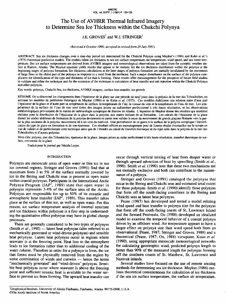
one or more isolated regions of open water or thin ice. We searched for an extended period of clear, cloud-free weather during which the formation of a freshly generated ice surface was observed in the polynya and during which one could be certain no snowfall occurred. For the period selected, the Chukchi Polynya formed between Icy Cape and Cape Lis- bume. It extended 125 km south from Icy Cape, and its great- est width was 20 km. Water depth in this region is 15-25 m. The polynya (Figs. 2, 3, 4) displayed the banding or striping parallel to the coast typical of many polynyas. This banding or striping is generally thought to be caused by the episodic freezing of the sea surface as the polynya opened under the influence of wind and reflects differences in ice thicknesses and ice surface temperature within the polynya. The width of the strips and their gray value appeared to change with time.

In the discussion that follows we will 1) justify the identification of the distinctive striping observed within the polynya on the AVHRR imagery as thin ice of graded thicknesses, 2) describe the precision and accuracy of the temperature assignments to the thin ice within the strips, 3) evaluate the choices of the temperature and wind variables from those recorded at the synoptic weather stations at Barrow and Kotzebue, and 4) examine the use of the ice thickness equations described previously.

METHODOLOGY

An exceptionally cloud-free period on the Chukchi coast between Barrow and Pt. Hope was identified for 12-21 March 1987. Nine AVHRR computer-compatible tapes (CCTs) for the polar-orbiting NOAA-09 and NOAA-10 satellites (Table 1)

FIG. 2. The Chukchi Polynya as it appeared on 15 March 1987 on the AVHRR thermal infrared band. This image has been enhanced to reveal the internal structw of the polynya; features within the pack ice and fast ice and on land are unenhanced. The four enhanced strips have median values of -7.6OC (black), -10.2"C (dark gray), -12.9"C (light gray), and -15.5OC (white) and display the warmest temperatures in the image. Temperatures in the unenhanced part of the image are <-19.OoC.

132 / J.E. GROVES and W.J. STRINGER

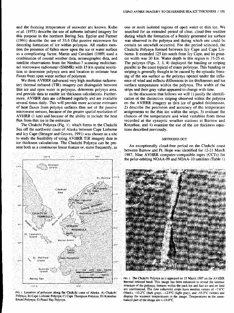
FIG. 3. The Chukchi Polynya as it appeared on 15 March 1987 in the AVHRR visible band. This image is unenhanced.

were ordered from the Satellite, Data, and Information Service's National Climatic Data Center in Washington, D.C. (NESDIS).

The nine CCTs were analyzed at the Alaska Data Visual- ization and Analysis Laboratory (ADVAL), located at the Geophysical Institute, University of Alaska Fairbanks. Each image was geo-registered to an Alaska Map E base. The pri- mary analysis emphasis was on the thermal infrared band (10.3-1 1.5 Pm), which was used to obtain surface temperatures of ice forming on the surface of the polynya. However the visible band (0.58-0.68 gm) and near infrared band (0.72-1.1 Pm) were also inspected. Visible and near infrared imagery were available for 7 of the 9 images. As the 17 and 21 March images were obtained during the night, only thermal imagery was use- ful. The remaining images were acquired at approximately the same time each day. This gave an approximately 24 h spacing between each scene. The 13 and 14 March images were consecutive images. Temperature calibration for each of the nine CCTs was accomplished using the method described by Lauritson et al. (1979).

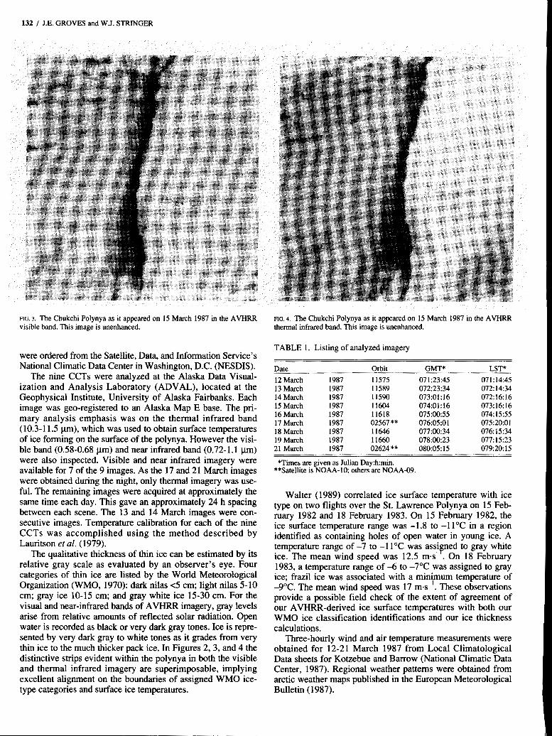
The qualitative thickness of thin ice can be estimated by its relative gray scale as evaluated by an observer's eye. Four categories of thin ice are listed by the World Meteorological Organization (WMO, 1970): dark nilas 4 cm; light nilas 5-10 cm; gray ice 10-15 cm; and gray white ice 15-30 cm. For the visual and near-infrared bands of AVHRR imagery, gray levels arise from relative amounts of reflected solar radiation. Open water is recorded as black or very dark gray tones. Ice is represented by very dark gray to white tones as it grades from very thin ice to the much thicker pack ice. In Figures 2, 3, and 4 the distinctive strips evident within the polynya in both the visible and thermal infrared imagery are superimposable, implying excellent alignment on the boundaries of assigned WMO ice- type categories and surface ice temperatures.

FIG. 4. The Chukchi Polynya as it appeared on 15 March 1987 in the AVHRR thermal infrared band. This image is unenhanced.

TABLE 1. Listing of analyzed imagery

Date Orbit GMT* LST* 12 March 1987 11575 07 1 :23:45 07 1 : 14:45 13 March 1987 1 1589 072:23:34 072:14:34 14 March 1987 11590 073:01:16 072:16:16 15 March 1987 11604 074:01:16 073:16:16 16 March 1987 11618 075:00:55 074: 15:55 17 March 1987 02567 ** 076:05:01 075:20:01 18 March 1987 11646 077:00:34 076:15:34 19 March 1987 11660 078:00:23 077:15:23 21 March 1987 02624 ** 080:05:15 079:20:15

**Satellite is NOAA-IO; others are NOAA-09. *Times are given as Julian Day:h:min.

Walter (1989) correlated ice surface temperature with ice type on two flights over the St. Lawrence Polynya on 15 Feb- ruary 1982 and 18 February 1983. On 15 February 1982, the ice surface temperature range was -1.8 to -11°C in a region identified as containing holes of open water in young ice. A temperature range of -7 to -1 1°C was assi ned to gray white ice. The mean wind speed was 12.5 mes . On 18 February 1983, a temperature range of -6 to -7°C was assigned to gray ice; frazil ice was associated with a minimum temperature of -9°C. The mean wind speed was 17 m-s". These observations provide a possible field check of the extent of agreement of our AVHRR-derived ice surface temperatures with both our WMO ice classification identifications and our ice thickness calculations.

Three-hourly wind and air temperature measurements were obtained for 12-21 March 1987 from Local Climatological Data sheets for Kotzebue and Barrow (National Climatic Data Center, 1987). Regional weather patterns were obtained from arctic weather maps published in the European Meteorological Bulletin (1987).

-F


The precision of the AVHRR temperature calculations derives from the method of temperature calibration described in Lauritson et al. (1979). Each satellite has a unique calibration curve from which a look-up table is created, where the radiance values are recorded as integer values related to temperature differences of about 0.15"C. Variation of the calibration coefficients used for calculation of the calibration curve cause a variation of kO.05"C for each radiance value for both NOAA-09 and NOAA-10 imagery. Thus the assertion that the sea ice surface temperature reported for each band of thin ice is precise to M.2"C is justified for each NOAA satellite scene. However, problems still exist comparing temperature assignments between satellites, implying that despite the precision of 0.2"C, the actual temperature values are not that accurate.

There are several approaches for assessment of the accuracy of the temperatures. The temperatures derived from AVHRR data are brightness temperatures and do not match true surface temperatures except under special circumstances. Li (pers. comm. 1991) states that the emissivity for ice and water near the freezing point is 0.998, and AVHRR brightness temperatures do approximate the true surface temperature. However, for Barrow and Kotzebue, assuming an emissivity of 0.97 for terrestrial snow, the AVHRR brightness temperatures for the snow surface are approximately 1.5"C lower than the synoptic air temperatures. We compared the AVHRR terrestrial snow surface brightness temperatures with synoptic air temperatures recorded at Barrow and Kotzebue near the time of the passes, and the AVHRR brightness temperatures were 2-6°C lower. Barton et al. (1989) state that it is possible to determine SST for open water in mid-latitudes under clear sky conditions to an accuracy of 0.7"C.

Our temperature assignments for the polynya strips may be as accurate as the 0.7"C observed at mid-latitudes and are likely within the +2"C accuracy implied by both the theoretical and observational differences noted between AVHRR brightness temperatures and true ground temperatures at high latitudes. For this study our temperature assignments are more likely to be 2°C lower than the true ground temperature, not 2°C higher.

The sources of meteorological data closest to the Chukchi Polynya are the synoptic weather stations operated by the National Weather Service at Barrow and Kotzebue, Alaska. Two western branches of the Brooks Range, the Delong and Baird mountains, separate Kotzebue from Barrow and from the Chukchi Polynya, which is located between Icy Cape and Cape Lisburne on the western edge of a flat arctic plain (Fig. 1). During the spring this region is often covered by large regional weather systems, creating fairly uniform temperatures across the arctic plain. Thus the record at Barrow (though 250 km north of the Chukchi Polynya) was selected as being more likely representative of conditions off the coast between Pt. Lay and Icy Cape than the Kotzebue data.

Polar arctic weather maps published in the European Meteorological Bulletin (1987) prepared by the German Weather Service were inspected for two purposes. Surface charts at OOO GMT were used to determine wind direction at the times of the satellite passes (Table 1). These passes occurred between 2300 of the previous day and 0100 of the day of the weather map. The first objective was to correlate opening and closing of the Chukchi Polynya with wind direction in a broad qualitative way (Table 2). Table 2 suggests that polynya opening and closing are affected by wind and temperature variables averaged over a 24 h period prior to the pass. The second objective

TABLE 2. Qualitative history of the opening and closing of the Chukchi Polynya, 2-21 March 1987

Wind Date direction from* Temp C** Status of polynya formation***

2 March 3 March

4 March

5 March

6 March 7 March

8 March 9 March

10 March 1 1 March 12 March 13 March 14 March 15 March 16March

17 March

18 March

19 March

20 March

21 March

East East

Southeast

south

West West

Southeast Southeast

South West West East East Northeast Northeast

Northeast

Northeast

Northeast

Northeast

Northeast

-3 2 -33

-3 1

-27

-19 -19

-22 -14

- 8 -17 -23 -23 -27 -26 -28

-3 1

-30

-27

-32

-3 1

Polynya starting to open Open and banded from Lisburne

Open and banded from Lisbume

Open and banded from Lisburne

Closed, but cloudy Open north of Icy Cape; freezing

over Cloudy Open north of Icy Cape with

Cloudy Closed; lead not polynya Closed; lead not polynya Polynya starting to open Polynya opening Polynya at its maximum size Polynya starting to close; floes

Polynya starting to close; floes





to Barrow

to Barrow

to Barrow

freezing leads

move to SW

move to SW

move to SW

move to SW

move to SW

move to SW

*Wind direction for Barrow and the Chukchi coast from the European

**Temperatures from monthly summary Local Climatic Data sheets Meteorological Bulletin G m 2 3 59.

GMT23 59. ***Observations from photographic record of AVHRR imagery.

was to provide independent confirmation of the suitability of representing conditions on the Chukchi coast with the mean daily averaged wind vectors observed at Barrow. The quantitative wind vectors at Barrow agree well with the directions indicated on the weather maps.

Based on the evaluations described above, we selected mean daily air temperatures and wind vectors derived from the Observations at 3-hour Intervals Table in the Local Climato- logical Data Sheets. Averaging was performed over the 24 h period immediately preceding the satellite pass.

Figure 5 displays the mean daily wind vectors at Barrow for the study period. The vectors were compiled from the Observations at 3-hour Intervals Table. The 24 h period used for the averaging was the day (GMT) previous to the average time of the satellite passes, most of which occurred an hour before or after 2400.

Prior to the study period, inspection of the Barrow record revealed that the first week of March 1987 was cold, the second week was warmer, and the study period itself was very cold and characterized by a cooling trend - a pattern in the Kotzebue record as well. Figure 6 displays the temperatures recorded at the synoptic weather stations at Barrow and Kotzebue for the study period near the time of each satellite pass. The two plots define the limits of the temperature one might expect to find at the Chukchi Polynya for the study period.


An ice surface temperature analysis was performed utiliz- ing a discrete series of gray-scale values stepping in increments of 2°C for images of the Chukchi Polynya. The series encom- passed a linear gray-scale temperature range from -2.9"C to -3O.O"C. This enhancement was used for ice thickness calculations because it defined unique regions of ice with a known average sea ice temperature. Figure 2 illustrates how the striping appeared in the thermal band on 15 March. The tempera-

WIND DIRECTION AND SPEED (cm/sec) RECORDED AT BARROW BETWEEN MARCH 10 AND 2 1. 1 9 8 7 (GMT)

MARCH 10 MARCH 11 MARCH 1 2 MARCH 15

MARCH 18 MARCH 19 MARCH 20 MARCH 21

SPEED. 225crnk.e~ PER DIVISION DIRECTION: ARROW POINTS IN DIRECTION TOWARD WHICH THE WIND IS BLOWING

FIG. 5. Daily modal wind direction at Barrow.

TEMPERATURE CHANGE AT BARROW AND KOTZEBUE BETWEEN MARCH 10 AND 21, 1 9 8 7

- - - Kotzebue

0 NOAA-IO Satellite PSS

0 NOAA-09 Satellite Parr

\ \ \ \

' I

- 34 1 1 1 1 1 1 1 1 1 1 1 1

10 11 12 13 14 15 16 17 18 19 20 21 (GMT) MARCH

Temperatures are selected as those closest to the time of satellite pass; dates are Greenwich Mean Time (CMT).

FIG. 6. Air temperatures at the Synoptic Weather Stations at Barrow and Kotzebue near the time of each satellite pass.

ture boundaries for the striping in Figure 2 are those chosen to display the strips clearly. This series consists of four equal steps between -6°C and -16.5"C.

Ice thicknesses were calculated using two models that allow such determinations based on observed ice surface temperatures (To). The first is that of Maykut (1986) and the second is from Kuhn et al. (1975).

Kuhn et al. model (1975): HK = - - KiK (TF - To)

Table 3 defines and compares the variables and coefficients used in each model.

The Maykut thickness model is a formulation of the empirical observation that good estimates of ice thickness can be obtained from computation of cumulative freezing-degree days alone (Anderson, 1961). The model states that heat loss at the upper ice surface must equal the heat gained at the upper surface by conduction from the lower surface through the thin ice layer (FcM):

where - (TF- To) = FcM; the conductive heat flux KiM

HM The constant (KIM) for the thermal conductivity of ice

yields a 24 h estimation of the ice thickness. The constant C,, which describes sensible and latent heat exchange, has a slightly higher value than that for sensible heat loss alone. Latent heat loss, while not negligible, is assumed to be minimal.

The Kuhn model assumes an equilibrium between heat conduction through the ice layer (FcK) and net total radiant heat exchange (FNT) and sensible heat loss at the upper ice surface PSI:

KiK - HK

KiK where - (TF - To) = FcK; the conductive heat flux HK

The constant (KiK) for the thermal conductivity of ice yields an instantaneous estimation of ice thickness. Latent heat exchange is considered negligible.

Kuhn et al. assign the value 1.6 x 10" calcm .s to FNp the net total (IR and solar) radiation balance at the ice surface. This value is derived from observations on T-3, an ice island that inhabited the polar ice pack for a number of years. Sensi- ble heat exchange, F,, is calculated by the equation in Table 3. Kuhn et al. assign the values recorded in Table 3 to the convective heat transfer coefficient (Ce), the density of air (p), and the specific heat of air (Cp). The temperature difference (To - Ta), the difference between sea ice surface temperature and air temperature, is treated as identical to the (To - T,) term in the Maykut model in that we use the mean daily air temperature at Barrow for T,. For wind speed U in rn-s" we use the mean daily wind vector at Barrow. For the convective heat transfer coefficient (Ce) we use the value (1.1 x observed by Walter (1989) in the St. Lawrence Island Polynya.

-2 -1

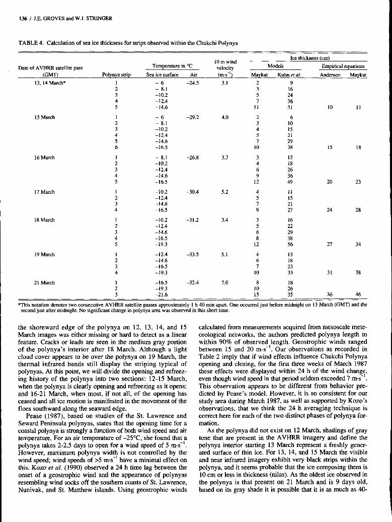
Using the median ice surface temperature values from each of the strips defining the discrete series and Maykut's and Kuhn er al.'s equations, ice thicknesses were calculated for all strips observed seaward of the fast ice. The visible and near- infrared bands were checked to establish that these strips cor- responded to open water, black ice, or thin ice and were not associated with the fast ice or pack ice. The values from each method of sea ice thickness calculation are compared in Table 4.

Cumulative ice growth calculations were made as an independent check on these models of the ice thickness. Maykut (1985) described empirical methods of calculating young ice growth from cumulative freezing-degree days (0). One freezing-degree day is defined as the difference between the freezing temperature of seawater and the mean daily temperature to the nearest "C. Two of these methods were used to estimate how much ice could have been generated during the opening of the shore lead to form the polynya during the 24 h period between 12 March and 13-14 March (i.e., the first day's ice growth) and how much would have been generated cumula- tively at the time of each satellite pass for the entire nine-day period. These are listed in Table 4.

The first method is a quadratic equation derived by Ander- son (1961) to fit field data from Greenland relating cumulative freezing-degree days (e) to measured ice thickness. This equation is valid for thicknesses (H) from 10 to 80 cm under conditions of minimal snow cover.

H2 + 5.1H = 6.70 8

Maykut presents the theoretical expression

H2 - H2, + (2k,/k,(H,) + 2k,/C,) (H - H$) = 2k,/pi L(0) where H, is the initial thickness of the ice, ki is the average thermal conductivity of the ice, k, is the thermal conductivity of the snow, pi is the density of ice, L is the latent heat of fusion, C, is a bulk transfer coefficient describing turbulent heat transfer between the ice and atmosphere, and H, is the snow depth.

With nominal values for the thermal properties and H, = H, = 0, the above equation is written as: H2 + 16.8H = 12.90; Maykut states that with no snow cover this equation predicts too rapid growth.

RESULTS

In this discussion we will 1) relate meteorological variables to polynya formation, 2) describe qualitatively the ice proper-


ties within the polynya that may be deduced from observation of AVHRR imagery, 3) discuss the capability of AVHRR to distinguish changes in ice thickness, and 4) discuss the ice thickness calculations in reference to two distinct periods of polynya formation.

The Chukchi Polynya is a latent heat polynya; its size and the motion of the ice at its seaward edge over time appear to be largely a reflection of the action of wind, although other factors such as air temperature probably play a significant role in its morphology. The relationship between polynya opening and closing and wind direction for the first three weeks in March is presented in Table 2. A wind from the east, southeast, or south results in opening of the polynya. A wind from the northeast results in southwestward motion of floes along the seaward (west) side of the polynya. These effects are evident within 24 h of the onset of the wind. On 12 March at 1445 AST the Chukchi Polynya was not present; in its place was a shore lead extending from Cape Lisbume to Icy Cape. On both the visible and near infrared imagery the interior region of the lead was very dark, implying open water or very thin ice. The borders of the lead were bright white and very distinct from the lead itself. On 13 March, some 24 h later, the lead had opened to the point that the Chukchi Polynya was formed, displaying the typical striped appearance of an opening polynya. The strip patterns seen on all three AVHRR bands for 13 March and for subsequent images were superimposable, implying excellent agreement among all three bands on the boundaries of the polynya and ice thickness categories within it. The boundary between the darker strips and very white tones, representing the pack ice, was very smooth and distinct. This description held for the 14 and 15 March images. Figures 2,3, and 4 illustrate the agreement on location of polynya striping in the different AVHRR bands. Figure 5 displays wind direction and speed for the study period. For 13- 22 March, excepting 14 March, the wind is from the northeast, which is normal for Barrow in March (Brower et al., 1988). On 14 March, the wind was from the east; its speed was 5-12.5 ms". On 16 March, the boundary between the pack ice and the interior of the polynya became more irregular. Several large floes at various positions along the seaward edge were identified and tracked. Between 12 and 15 March, no significant motion of floes was noted. On 16 March the floes began to move to the southwest, matching the northeasterly winds observed after 16 March. In some cases they moved 30 krnd". Significant southwesterly motion was observed through the 21st. On 18 and 19 March the very black strip characterizing

TABLE 3. Definition and Comparison of Variables and Coefficients used for Ice Thickness Calculations ~ ~~~~~ ~ ~ ~~

Maykut (1986) Kuhn er ai. ( 1975) Ice thickness (cm) H, }The cumulative ice growth in a 24 h period HK )The instantaneous ice thickness Thermal conductivity of ice K,, = 419.9 cal-cm"d0c" Ki, = 4.86 x c a l a n - l d " C ' Conductive heat flux FcM (calcm-*.d") F ~ , (calan-'.s") Freezing point of seawater or seawater temperature ("C) Ice surface temperature ("C) Air temperature ("C) Average transfer coefficient describing sensible and latent

Net total (IR and solar) radiation balance Sensible heat exchange Convective heat transfer coefficient Density of air Specific heat of air Wind speed (ms")

T, = -1.8oC TF = -1.8"C TO To Ta T.

heat exchange C, = 50 calcm".d""C-' - - FNT = 1.6 x IO4 cal.crn-'.s"

C, = 134 x

C, = 1004 J.deg-l.kg" U

Included in C, FS=C C,(T,-TJU - - p = 1.3 kg~rn-~ - -


TABLE 4. Calculation of sea ice thickness for strips observed within the Chukchi Polynya

10 m wind Ice thickness (cm)

Date of AVHRR satellite pass Temperature in "C velocity Models Empirical equations (GMT) Polynya strip Sea ice surface Air (ms") Maykut Kuhn et al. Anderson Maykut

13.14 March*

15 March

16 March

17 March

18 March

19 March

21 March

1 2 3 4 5

1 2 3 4 5 6

1 2 3 4 5

1 2 3 4

1 2 3 4 5

1 2 3 4

1 2 3

- 6 - 8.1 -10.2 -12.4 -14.6

- 6 - 8.1 -10.2 -12.4 -14.6 -16.5

- 8.1 -10.2 -12.4 -14.6 -16.5

-10.2 -12.4 -14.6 -16.5

-10.2 -12.4 -14.6 -16.5 -19.3

-12.4 -14.6 -16.5 -19.3

-16.5 -19.3 -21.6

-24.5

-29.2

-26.8

-30.4

-31.2

-33.5

-32.4

3.1 2 3 5 7

11

4.0 2 3 4 5 7

10

3.7 3 4 6 9

12

5.2 4 5 7 9

3.4 3 5 6 8

12

5.1 4 6 7

10

7.0 8 10 15

9 16 24 36 51 10

6 10 15 21 29 38 15

12 18 26 36 49 20

1 1 15 21 27 24

16 22 29 38 56 27

13 18 23 33 31

18 26 35 36

11

18

23

28

34

38

46

*This notation denotes two consecutive AVHRR satellite passes approximately 1 h 40 min apart. One occurred just before midnight on 13 March (GMT) and the second just after midnight. No significant change in polynya area was observed in this short time.

the shoreward edge of the polynya on 12, 13, 14, and 15 March images was either missing or hard to detect as a linear feature. Cracks or leads are seen in the medium gray portion of the polynya's interior after 18 March. Although a light cloud cover appears to be over the polynya on 19 March, the thermal infrared bands still display the striping typical of polynyas. At this point, we will divide the opening and refreezing history of the polynya into two sections: 12-15 March, when the polynya is clearly opening and refreezing as it opens; and 16-21 March, when most, if not all, of the opening has ceased and all ice motion is manifested in the movement of the floes southward along the seaward edge.

Pease (1987), based on studies of the St. Lawrence and Seward Peninsula polynyas, states that the opening time for a coastal polynya is strongly a function of both wind speed and air temperature. For an air temperature of -25OC, she found that 1" polynya takes 2-2.5 days to open for a wind speed of 5 ms- . However, maximum polynya width is not controlled by the wind speed; wind speeds of >5 m-s" have a minimal effect on this. Kozo et al. (1990) observed a 24 h time lag between the onset of a geostrophic wind and the appearance of polynyas resembling wind socks off the southern coasts of St. Lawrence, Nunivak, and St. Matthew islands. Using geostrophic winds

calculated from measurements acquired from mesoscale meteorological networks, the authors predicted polynya length to within 90% of observed length. Geostrophic winds ranged between 15 and 20 mas". Our observations as recorded in Table 2 imply that if wind effects influence Chukchi Polynya opening and closing, for the first three weeks of March 1987 these effects were displayed within 24 h of the wind change, even though wind speed in that period seldom exceeded 7 m-s" . This observation appears to be different from behavior predicted by Pease's model. However, it is so consistent for our study area during March 1987, as well as supported by Kozo's observations, that we think the 24 h averaging technique is correct here for each of the two distinct phases of polynya formation.

As the polynya did not exist on 12 March, shadings of gray tone that are present in the AVHRR imagery and define the polynya interior starting 13 March represent a freshly generated surface of thin ice. For 13, 14, and 15 March the visible and near infrared imagery exhibit very black strips within the polynya, and it seems probable that the ice composing them is 10 cm or less in thickness (nilas). As the oldest ice observed in the polynya is that present on 21 March and is 9 days old, based on its gray shade it is possible that it is as much as 40-

50 cm thick where it is piling up at the southwestern end; yet there may be ice even less than 15 cm thick (i.e., nilas and gray ice only) in small pockets at the northeast end of the polynya. The excellent agreement among the visible, near infrared, and thermal infrared bands for the boundaries of the internal structure of the polynya at the beginning of the study period con- firm that one can use the visible and near infrared bands to check validity of the polynya boundaries indicated by the thermal infrared; and in the absence of visible imagery, such as in the case of nighttime images, the thermal infrared alone gives valid boundaries.

Two approaches were investigated concerning the capability of the AVHRR thermal infrared imagery to associate the temperature changes of identifiable strips within the polynya with the growth of a quantifiable thickness of ice. We estimate our temperature assignments for the various ice strips to be good to +2”C for the purpose of comparing one image with another. (Relative temperature assignments within each indi- vidual image are much better.) This uncertainty amounts to +lo%, or 0.2 cm for a 2 cm ice thickness as calculated from the Maykut (1986) thickness model.

The second approach asks how much ice can be generated for a heat loss to the atmosphere represented by an air temperature change of 1OC. The value assigned to the latent heat of ice is important, since, at least for the 12-15 March period, we are definitely observing the active formation of thin ice. Maykut’s empirical ice growth equation (1985) for relating ice thickness to degree days assumes a value of 72 cal-g” for the latent heat of ice of 4%0 (approximately 13% of the salinity to be expected off Pt. Lay in March [32.5%0; Coachman et al., 19751) and assumes the formation of a solid sheet of ice. Solving the equation H2 + 16.796 H = 12.9 8 for 8 = lOC-day, one calculates that 1°C-day results in the formation of 0.7 cm of thin ice. The initial stage of freeze-up for a polynya under windy conditions has been observed to be the formation of frazil ice (Bauer and Martin, 1983). If we assume that the “thin ice” we observe forming 12-15 March is a water/ice mixture containing 50% frazil ice with an effective latent heat of 50% of 72 calvg”, the Maykut empirical ice growth equation yields the result that 1’C-day forms 1.4 cm of frazil. One concludes that whatever the type of ice forming at the surface of the polynya, AVHRR imagery in theory ought to be able to detect ice growth increments as small as 1 cm. We estimate our experimental uncertainty for ice growth at f 1 cm.

Let us compare the adequacies of the Maykut and Kuhn et al. thickness models to describe ice thickness within the Chukchi Polynya. The period 13-15 March is a simple case of the polynya opening and new ice forming in distinctive bands parallel to the retreating seaward edge of the polynya. The critical issue is the nature of the ice forming. Bauer and Martin (1983) differentiate between ice formed in calm conditions and that formed under the presence of high winds (2 10 m.sec”). For calm conditions a skim is formed horizontally. Bauer and Martin’s ice growth model is restricted to wind speeds 2 10 m d . In the first phase, winds 1 10 mes” result in the formation of frazil ice, which is advected downwind, where it piles up against the seaward edge of the polynya. In the second phase of ice formation, the accumulated frazil ice forms a layer of grease ice, which advances upwind. For 13-15 March the wind speed was 3-4 m-s-’. Pease (1987) states that h y

-model for polynya size is not valid for wind speed I 5 m.s- . These model studies suggest that our study period (with low


wind speed) occurred during a transition from calm conditions (where solid ice forms as a skim on the surface and contributions from latent heat of formation of ice are most influential in determining ice thickness) to high wind conditions (where ice thickness is characterized primarily by the action of wind piling up frazil ice).

One can account for this difference in the nature of the ice layer either by changing the effective latent heat of ice by a factor representative of the composition of water and frazil ice in the ice layer or by stating, as Kuhn does, that the latent heat of ice is negligible. The Maykut thickness model and the Ander- son and Maykut empirical ice growth equations, in effect, assume the formation of solid ice, and the Kuhn et al. equation, by neglecting the latent heat of ice, behaves as an estimation of the thickness of a mixed frazil ice/water layer, although this was probably not the intention of Kuhn et al. in formulat- ing the equation.

We assume that the first period of ice formation (12-15 March) is characterized by calm wind, and ice growth occurs as a skim of solid ice. The Maykut ice thickness model, which accounts for the latent heat of ice and discounts the effect of wind speed, ought to be best suited for ice thickness calculations for this period. This is supported by the observation that the Maykut thickness calculations agree well with the appearance and gradual freezing of nilas recorded in the visual and near infrared imagery.

The second period of ice growth (16-21 March) is also characterized by low wind speed. However, ice growth is complicated by the movement of ice floes to the southwest. Bauer and Martin’s model (1983) calculates the frazil ice depth for a wide range of wind speed, but only for a narrow range of fetch (50-500 m). We hypothesize that low wind speed (e 5 mas- ) from a direction parallel to the 125 km axis of the polynya (in contrast to perpendicular to the axis, as on 12-15 March) represents such a large fetch that even very low winds can cause the build-up of considerable frazil as well as the movement of the floes. Thus for this period, the Kuhn et al. equation might by coincidence approximate the frazil depth. Nevertheless, even in this second period, portions of the surface of the polynya must be covered with ice solid and thick enough to yield surface temperatures -6°C and lower.

For the first day’s ice growth, Anderson’s and Maykut’s empirical degree-day growth equations give 10 cm and 11 cm respectively. For the first day’s polynya opening, the oldest (most seaward) strip within the polynya is 11 cm thick using the thermal data applied to Maykut’s ice thickness model, which agrees with the 10-1 1 cm predicted empirically for the ice that grew in the 24 h period beginning with the opening of the lead. These calculations agree well because they represent the growth of a thin skim of ice under calm conditions. Kuhn et al.’s thickness model yields a thickness of 5 1 cm.

At the time of the second day’s observation, the oldest identifiable strip is 10 cm thick using Maykut’s thickness model and 38 cm thick using Kuhn et al. For the accumulated ice growth over the two-day period, Maykut’s empirical ice growth equation gives 18 cm and Anderson’s 15 cm. As the ice formation conditions are still calm, the Maykut thickness model and the Anderson and Maykut empirical ice growth equations should agree better. Agreement may be poor because we are unable to identify the two-day-old ice strip that has been piled up at the seaward edge of the polynya. The Maykut thickness model follows an identifiable ice strip as it moves in the expansion of the polynya.


For 16 March, the first day of the second stage of polynya formation, we note the start of southward movement of several large floes. This movement must also be accompanied by build-up of ice through pile-up and rafting at the southwestward end of the polynya. While the thermal infrared analysis still reveals strips of ice parallel to the coast and broader at the southern end of the polynya, the thickness distribution within some strips must be deformed by the movement of the floes within the polynya. On 16 March, Maykut’s ice thickness model gives 12 cm for the thickness of the oldest observable strip, Kuhn et ai. 49 cm, and the cumulative ice growth equations 20 and 23 cm. On 21 March, Maykut’s ice thickness model gives 15 cm for the thickness of the oldest strip, Kuhn et ai. 35 cm, and the cumulative ice growth equations 36 and 46 cm. Because of the above complications associated with polynya formation, it is not easy to judge which model most closely models ice thickness within the polynya.

The Maykut ice thickness model is inadequate to determine ice thickness under these conditions because it presumes the formation of a skim of solid ice under low wind conditions. Bauer and Martin’s (1983) study implies that for a fetch of 125 km considerable formation of frazil can accumulate even under low wind speed (< 5 mms-’). Maykut’s ice thickness model is not suited for frazil ice.

DISCUSSION

A comparison of our gray scale interpretation of the AVHRR imagery and the associated calculated ice thicknesses with Walter’s (1989) field observations of the St. Lawrence Island Polynya is given in Table 5. Table 5 reveals that what we labeled as dark nilas (I 5 cm) is calculated to be I 5 cm thick using the Maykut model and has a temperature of -6 to -10.2”C for both 13 and 15 March. Walter (1989) labeled as gray young ice (10-15 cm thick) ice having surface temperatures of -6 to -7°C. Walter’s ice thicknesses and ice surface temperatures are in better agreement with Kuhn et al.’s calculations (Table 4).

We think the closer agreement of Maykut’s thickness calculations with the cumulative ice calculations confirms these calculations, and our assignments of ice type according to the WMO standard are better estimations of ice thickness for the Chukchi Polynya for the period 13-15 March than Kuhn et d ’ s

thickness calculations and Walter’s field observations of ice quality of the St. Lawrence Polynya. This is because the surface of the polynya from 13 to 15 March is likely less hetero- geneous than the polynya surface observed by Walter.

For the period 16-21 March, many discrepancies between ice thickness calculations, cumulative ice thicknesses, and gray scale interpretation exist. Walter (1989) describes the surface of the St. Lawrence Island Polynya as highly heteroge- neous and composed of frazil ice, open water, frozen holes, and the previously mentioned gray young and white young ice; it is subjected to winds of 12-17 mas”. This type of hetero- geneity most likely characterizes the surface of the Chukchi Polynya as well, especially for the period 16-21 March. Walter (1989) also determined bulk heat transfer coefficients for the ice he observed; they ranged from 0.6 x for frazil to 1.1 x

for the other forms of ice. Therefore, we chose Walter’s value (1.1 x for the bulk heat transfer coefficient in Kuhn et al.’s ice model, rather than Pease’s (1987) of 2.0 x

for o en water in polynyas or Kuhn et al.’s (1.4 x to 1.7 x 10- ) for ice in leads. Even taking into account the above factors, assessment of the performance of either ice thickness model for the latter period is difficult.

After 16 March the cumulative ice thickness calculations are in better agreement with the Kuhn et ai. model thicknesses than with the Maykut model thicknesses (Table 4). This is most likely because we are no longer able to identify the oldest strips of ice. However, it is not possible to correlate ice surface temperatures of the strips with the temperature ranges Walter observed associated with frazil and gray young and gray white ice in the St. Lawrence Island Polynya.

The Kuhn et al. ice thickness model is intriguing in that, unlike the other models, as it is sensitive to wind speed, it may mimic frazil ice thickness. However, studies such as Bauer and Martin’s (1983) document that the factors determining frazil or grease ice depth depend on many more factors than wind speed. Field observations, such as Walter’s for the St. Lawrence Island Polynya, document the extent of ice type variability that can occur within polynyas. Cumulative ice thickness equations that measure the thickness of relatively static ice are inappropriate for ice undergoing considerable deformation, such as during 16-21 March. We conclude that we cannot select one method of thin ice calculation as superior to the others for the period 16-21 March.

9

TABLE 5. Comparison of Chukchi Polynya AVHRR ice surface temperatures and associated ice thicknesses with gray scale assignments from the WMO classification and Walter’s field observations at St. Lawrence Polynya

Walter (1989) Chukchi Polynya, 13 March 1987 (St. Lawrence Polynya) Polynya strip temperature (“C) Thickness (cm) using Maykut (1986) WMO (1970) classification gray young ice -6 to -7°C 10-15 cm thick whlte young Ice -7 to 11°C 15-30 cm thick

- 6.0 - 8.1 -10.2 -12.2 -14.6

2 3 5 7

1 1

dark nilas 1 5 cm

light nilas 5-10 cm

Walter (1989) Chukchi Polynya, 15 March 1987 (St. Lawrence Polynya) Polynya strip temperature PC) Thickness (cm) using Maykut (1986) WMO (1970) classification

gray young ice -6 to -7°C - 6.0 2 dark nilas 10-15 cm thick - 8.1 3 S 5 c m whlte young Ice -7 to 1 l0C -10.2 4 15-30 cm thick -12.4 5 light nilas

-14.6 7 5-10 cm -16.5 10

Finally, most studies of polynyas have focused on latent heat polynyas formed under wind speeds of at least 5 mes" and more frequently 10 m-s". Brower et al. (1988) document the most frequent winds recorded at Barrow, Pt. Lay, and Cape Lisburne in the range of 5-8 m-s". Investigations involv- ing polynyas in the Chukchi Sea will have to address low wind conditions.

CONCLUSIONS

The thermal infrared band of AVHRR imagery is shown to give realistic sea ice surface temperatures that can be used for thin sea ice thickness calculations. Maykut's (1986) ice thickness model relating air temperature, sea ice surface temperature, and seawater temperature to sea ice thickness is shown to give the most reasonable results for daily changes in thickness of the freshly generated ice surface of a polynya under the conditions that low wind speed (e 5 mns") and a small fetch limit the formation of frazil ice. This study implies that one may also be able to calculate frazil ice thickness from sea ice surface temperature. Field studies are needed to refine and expand the technique, especially for low wind speeds. Better correlations must be found between ice type or roughness and the bulk heat transfer coefficient.

ACKNOWLEDGEMENTS

This study was funded in part under Contract #59 ABNC-00045 by the Minerals Management Service, U.S. Department of the Interior, through an interagency agreement with the National Oceanic and Atmospheric Administration, U.S. Department of Commerce, as part of the Outer Continental Shelf Environmental Assessment Program.

REFERENCES

ANDERSON, D.L. 1961. Growth rate of sea ice. Journal of Glaciology

BARTON, I.J., ZAVODY, A.M., O'BRIEN, D.M., CULLEN, D.R., SAUNDERS, R.W., and LLEWELLYN-JONES, D.T. 1989. Theoretical algorithms for satellite-derived sea surface temperatures. Journal of Geophysical Research 94:3365-3375.

BAUER, J., and MARTIN, S. 1983. A model of grease ice growth in small leads. Journal of Geophysical Research 88(C5):2917-2925.

BROWER, W.A., BALDWIN, R.G., WILLIAMS, C.N., WISE, J.E., Jr., and LESLIE, L.D. 1988. Climatic atlas of the outer continental shelf waters

3:1170-1172.


and coastal regions of Alaska. Vol. III. Chukchi-Beaufort Sea. Anchorage: Arctic Environmental Information and Data Center, and Asheville: U.S. National Climatic Data Center.

COACHMAN, L.K., AAGAARD, K., and TRIPP, R.B. 1975. Bering strait; The physical oceanography. Seattle: University of Washington Press. 172 p.

EPPLER, D.T., and FARMER, L.D. 1991. Texture analysis of radiometric signatures of new ice forming in arctic leads. IEEE Transactions on

EUROPEAN METEOROLOGICAL BULLETIN. 1987. Offenbach am Main, Geoscience and Remote Sensing 2(2):233-241.

F.R.G.: German Weather Service, Central Ofice. I& (International Arctic Polynya Program). 1989. Fairbanks: Institute of

Marine Science, University of Alaska Fairbanks. KOZO, T.L., FARMER, L.D., and WELSH, J.P. 1990. Wind-generated

polynyas off the coasts of the Bering Sea islands. In: Ackley, S.F., and Weeks, W.F., eds. Proceedings of the W.F. Weeks Sea Ice Symposium, Sea Ice Properties and Processes. CRREL Monograph 90-1 : 126-1 32.

KUHN, P.M., STERNS, L.P., and RAMSEIER, R.O. 1975. Airborne infrared imagery of arctic sea ice thickness. NOAA Technical Report ERL. 331- APCL 34. Boulder: U.S. Department of Commerce, NOAA, Environ- mental Research Laboratories.

LAURITSON, L., NELSON, G.J., and PORTO, F.W. 1979. Data extraction and calibration of TIROS-N/NOAA radiometers. NOAA Technical Memorandum NESS 107.73 p.

MARTIN, S., and CAVALIERI, D.J. 1989. Contributions of the Siberian shelf polynyas to the Arctic Ocean intermediate and deep water. Journal of Geophysical Research 94(0):12725-12738.

MAYKUT, G.A. 1985. The ice environment. In: Homer, R.A., ed. Sea ice biota. Boca Raton: CRC Press Inc. 21-82.

. 1986. The surface heat and mass balance. In: Untersteiner, N., ed. Geophysics of Sea Ice. NATO Advanced Science Institutes Series B, Physics, Vol. 146. New York Plenum Press. 395-463.

NATIONAL CLIMATIC DATA CENTER. 1987. Local Climatological Data. Asheville, North Carolina: U.S. Department of Commerce, NOAA.

OU, H.W. 1988. A time-dependent model of a coastal polynya. Journal of Physical Oceanography 18:584-590.

PEASE, C.H. 1987. The size of wind-driven coastal polynyas. Journal of Geophysical Research 92(C7):7049-7059.

SMITH, S.D., MUENCH, R.D., and PEASE, C.H. 1990. Polynyas and leads: An overview of physical processes and environment. Journal of Geophysical Research 95(C6):9461-9479.

STRINGER, W.J., and GROVES, J.E. 1988. A study of possible meteorological influences on polynya size. Fairbanks: Geophysical Institute, Uni- versity of Alaska Fairbanks, NOAA-OCS Contract No. ABNC-60041, November 1988.

STRINGER, W.J., and GROVES, J.E. 1991. Location and areal extent of polynyas in the Bering and Chukchi seas. Arctic 44 (Supp. 1): 164-171.

WALTER, B.A. 1989. A study of the planetary boundary layer over the polynya downwind of St. Lawrence Island in the Bering Sea using aircraft data. Boundary-Layer Meteorology 48:255-282.

WMO. 1970. Sea-Ice Nomenclature. No. 259, TP 145. Geneva: Secretariat of the World Meteorological Organization.

The Use of AVHRR Thermal Infrared Imagery to Determine …pubs.aina.ucalgary.ca/arctic/Arctic44-S-130.pdf · to Determine Sea Ice Thickness within the Chukchi Polynya ... Polynyas

Documents