TEXAS STATE BOARD OF WATER ENGINEERS Hal A. Beckwith, Chairman Andrew P. Rollins, Member James S. Guleke, Member THE UNIT HYDROGRAPH - ITS CONSTRUCTION AND USES Roy C. Garrett - Hydraulic Engineer Arthur H. Woolverton - Chief Hydraulic Engineer August, 1951

Welcome message from author
This document is posted to help you gain knowledge. Please leave a comment to let me know what you think about it! Share it to your friends and learn new things together.
Transcript
TEXAS STATE BOARD OF WATER ENGINEERS
Hal A. Beckwith, Chairman
Andrew P. Rollins, Member
James S. Guleke, Member
THE UNIT HYDROGRAPH -
ITS CONSTRUCTION AND USES
Roy C. Garrett - Hydraulic EngineerArthur H. Woolverton - Chief Hydraulic Engineer
August, 1951
FOREWORD
The unit hydrograph theory has received the attention of eminent hydrolo-gists since its introduction in 193 2. A number of articles concerning the subjectare to be found in the literature The information contained herein regardingthe unit hydrograph and its uses is presented with the hope that it will aid inengineering studies in the field of hydrology.
THE UNIT HYDROGRAPH - ITS CONSTRUCTION AND USES
INTRODUCTION
8A hydrograph of a stream as defined by Wisler and Brater is a graphical
representation of its fluctuations in flow arranged in chronological order. A
complete hydrograph shows every minor variation in flow and can therefore be
obtained only from an instrument that continuously records these changes, for
no stream is constant in flow even for short periods of time. Frequently,
however, such continuous records are not available and either instantaneous, or
mean daily readings, must be used in preparing the hydrograph. For instance,
the stream discharge records as given in the U. S. Geological Survey Water
Supply Papers are mean daily discharges. The beginning of the flood discharge
during the 24 hour period, the amount of the peak discharge and the time the
peak occurred are not commonly available in these records. Similarly the pre
cipitation records as published by the U. S. Weather Bureau usually give the
total precipitation for a 24 hour period. Thus it is not possible to tell from
these records the time a rain commences, when it ended, or the rate at which it
fell. Neither is it possible to tell with any degree of accuracy its direction of
travel across a watershed.
Naturally, if all of the factors mentioned above were known, a much more
accurate hydrograph could be produced* In constructing stream hydrographs,
judgement and experience must sometimes be used to overcome this lack of
information.
THE UNIT HYDROGRAPH
5The unit hydrograph, or unit graph, as defined by Sherman is a graph
representing 1, 00 inch of runoff from a watershed. This unit graph may be
-2-
prepared from a known hydrograph, and may then be used to compute a hydro-
graph of runoff for this area for any particular storm or sequence of storms
of any duration or intensity over any period of time.
Construction of the Unit Hydrograph
For simplicity of presentation the procedure for constructing the unit
hydrograph will be given step by step, and the construction of a unit hydro-
graph for Richland Creek in Navarro County, Texas, will be used as an example.
The steps in the construction of the unit hydrograph are as follows:
1. Selecting typical storm data.
Search the rainfall and stream discharge records of the watershed in
question for an isolated 24 hour rain storm which covers the area fairly
uniformly and which produces a rather large discharge. (Preferably,
but not necessarily, over 1. 00 inch of runoff over the watershed. ) It is
preferable that the flow of the stream be low, or normal, prior to the
rain, and that no additional rain fell during the flood runoff. Sherman
gives methods for separating the runoff resulting from antecedent and
subsequent rainfall, but these will not. be presented in this simple dis
cussion.
2. Obtaining the average rainfall over the area.
On a map, or map overlay, trace out the watershed in question. Locate
the gaging station and the precipitation stations in, and surrounding, the
area on the overlay. One of the standard methods of converting gage meas
urements to areal averages should be used to give the average depth of
precipitation over the area. Most good hydrology books will give a discussion
-3-
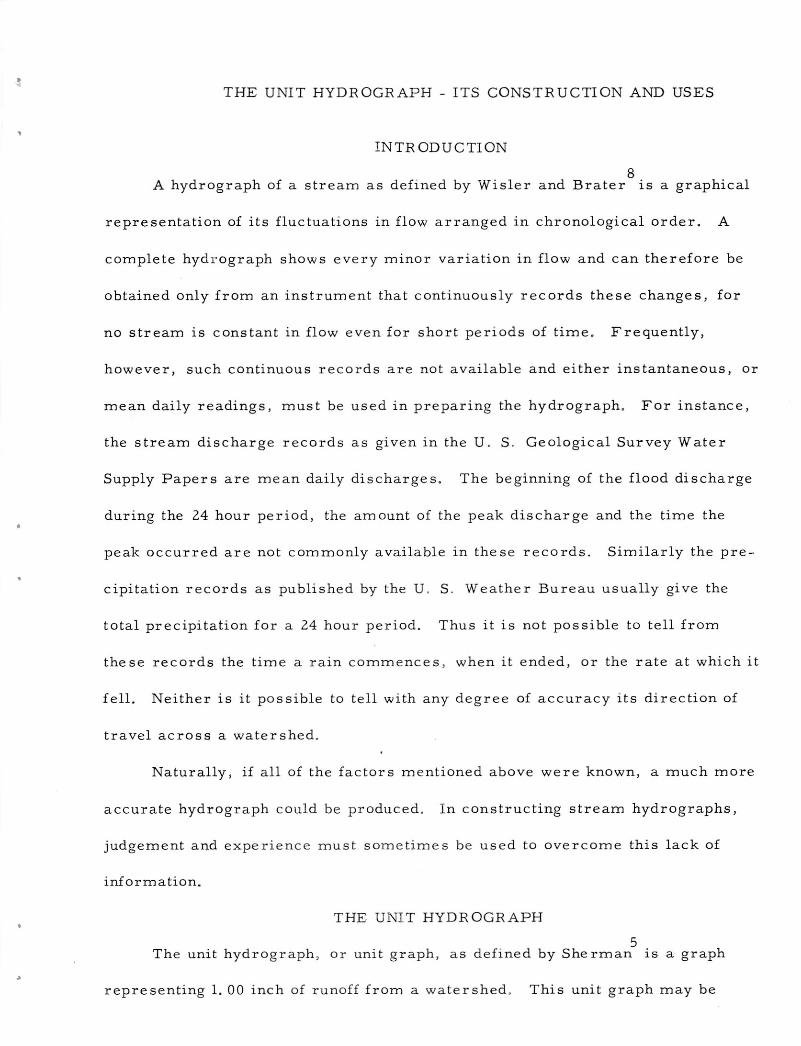
of these methods. Thiessens method was used on the Richland Creek area
because it is more accurate than the arithmetical mean method, yet is
simpler than the isohyetal map method. A Thiessen network is constructed
by locating the stations on a map and drawing the perpendicular bisectors
to the line connecting the stations. The polygons thus formed around each
station are the boundaries of the effective area assumed to be controlled
by that station. The area governed by each station is planimetered and
expressed as a percentage of the whole area. In the Richland Creek water
shed 25 percent of the area is closer to the Mexia gage than to any other
station, 38 percent closer to the Hillsboro gage and 37 percent closer to
the Corsicana gage as shown by Figure 1. It can be seen that in this method
the gages at Waco and Waxahachie should not be considered. Weighted
average rainfall for the basin is computed by multiplying each station's
precipitation by its assigned percentage of area and totaling as shown in
Table I. The use to be made of this weighted precipitation will be discussed
later.
TABLE I
WEIGHTED RAINFALL OVER
RICHLAND CREEK DRAINAGE AREA FOR SELECTED STORMS
Percent of Weighted
Gage R ainfall in in. area R ainfall (in. )March 7, 1947
Corsicana 1.36 37 . 50
Mexia 2. 00 25 . 50
Hillsboro 1. 15 38 .44
May 11-13, 19481.44
Corsicana 5. 86 37 2. 17
Mexia 2. 90 25 . 73
Hillsboro 3. 70 38 1.41
4. 31
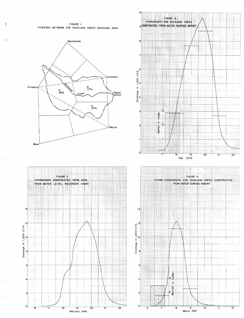
FIGURE I
THIESSEN NETWORK FOR RICHLAND CREEK DRAINAGE AREA
Hillsboro^- ~
Waco
18 19 20
February 1946
Mexico
<o ,£~
• • +rr-
PP 1 : : :
:::: i:r:'::::JRE >
B1CHL,
•--•
:~:~::::~VTER IURFA
—
::±:::::::
14 — \ ....
:::
: - —-+F Tr fftj W-:-.:'
. . A :::'2
.
/ \ H£
:/:: ::iV ::':H ri:
i $ .7::. .::
1 .
TTTi:i:'~T! TT 7™ "
' ! j: ;!::\
• • 1;...
/a?: . . !Ill . k. j ;.
\——. i$ • 1 z-—-V
$i'jM:- \% ii ; 1 . . .
Mi> ssii
i^lljIitJiUli...... y^
0 at!n 9
March 1947
10 I I
Dis
char
ge
in1
,00
0C
.FS
3&
9
Dis
harg
ein
1,0
00
C.F
S.
Dis
char
gein
1,0
00
C.F
S
;_•R
ainf
all
inin
eh
is
_
—t-—
.;'
{••:•
::::!:::::
•:|:
:•:•
:::.
::::
:::::
::::::
::r:—
rrj_
_
^^
*K
'
S-
::::
.::
::~
—f—
ift-
e—_
._
^:
:•
••
••
i
1::-
:i!i
iii:
:::
::::
::::
::::
::::
:i
_
::tf
:"";
:~-j
.i:
~r-^
^;:
—•
,
—.
z^rr
p~
.1
•j—
j.
——
—.
ml
^—
-"•
::::
:::::::::
:::
::::
.:::
:::
:-:r
r:^
:g-.
.
jSr.
.;.-..:,
;i;';::
:iijjH
i'inuf
ftIt^
:::;
*r^
-
o.......
—.—
_
nil
11
j-L-_
L_lJJ
_—
—_
i__
=
..
...
-
•
—J-
,.
,.
=====1==
[=======
=======l
===:
Ij
re
:|:"
"":::
-_
±±
:-
::::
••
J---
oto
*0
1
Dis
cho
rge
in1
,00
0C
.FS
.co
oro
•«»o
i
Htt
"if
':
:;
nL
::::
::::
::::
:::
::||
|#4-
=-
==H
-:-t|
:::±::::
:::El --
----
----
—j--
Uj:
•
<z
tfi>
X
'_
•iii
....
-
....._
...
—'.
.i.
-'itij
iiUiji 1
lil|M
ii,:-
z=
\
....
.:..
-4"
r:•;
•..
.
=^
-TT
i'!l
••
^E
8:
::::
::zi
rt+
r:.j
.-j—
,—1
_-
-C
l-
:::
#.....---
;:r
!;;
-r.~
^••;,
,frj
S3
i"
IC
I
.::::
-rg
r—
":••-.-
ri:
;:
|"•'
|~
^~
~-
-—•:
..:
—1
»-»
+•
.^-i
^-T
—X
-—^^
.-
a
!:
zr*
1 L—
——
"~1^
I'4=F
=—
[—
1.1;
:.::
i:::
:!:::
:r'1
=i
/
1/ i i L. l
_
:-:--_
-•
:.
::::::!::•
....
I.—
,—„
.........
.1
••
'::;;;
;ljh
:~~
™z=
=
11
••
::i:
j.::
i;::i:
:;:
::::;::::
iiiii
;:
::
.:'•
::":
::l~
:1
jzt
iz^
i":
discharge•in1,000C.FS.—nr\j<uoj
1tainfdllin
<»:::::;;
iniiiJ|i1p^=i ••••i••--i—i-1ii
j;•1r||]!•.1-1•
N"i£=^
*ii .
Jn.
\A
w\^S\;QrrT \^
•A~rv"\->i"'-3-__j—j_.j_,_|
•**—,^*v^;ii]1,:Lr..±..--:.I--.ij—I—J.
M—-i;'.-—,_J-_1JL4+--}---1{.'̂5.-LL_—[___;J.J—_^
-;-—r*JJ_—#1—,i|'|j/-^^
11QlliL^-iL_JF,x...—rH ;———'
/
'—7^:::3:5::
jf•Hri—>m-n
i,—-i—t—:—j——1-
•
....•i'|j1"-'[---$a:i-p——r±±:::
::••~r.::-H-.::_:oU'••**^
—
T":r•4'fa—'
-r-it—j>
,
PercentRunoff—upu^U01->JCO40
OOOOOOoooo
»ijd::jj|tjj:i::::|i^jH,!ii:;iiii::4:iiiiiiiii \LnfKtIn>.!3-•-iiiViiSi^iSiii.::i:i:iii: Iw\l•CEX:'.ill.:....£
!::XS£S5fev.::"iii:it••'••M3y4-m&=«••••••••••••v>«-•••• :::t*:::pr:%\:..:;-::r:\:;•;:.:-:>'c!!':::
V\i
Sfflffl!ml\1W TfE2,\*£rE:i:::::H:-JfL*\VA
TTi\'iH\1t—-i—t"VW
Dischargein1,000C.F.S
-4-
3. Plotting the storm hydrograph.
On arithmetical cross section, or hydrograph paper, plot the storm
hydrograph with flow in cubic feet per second as ordinates and days as
abcissae. The first step is to decide what scale to use; next make a bar
graph of the flow by drawing horizontal lines between the days representing
the mean discharge for the day. The area under each bar then represents
the total discharge for that day in second-feet days, and their sums would
represent the total discharge during the storm. It can be readily seen that
the rates during the day may vary appreciably from the mean daily dis
charge rate.. The hydrograph of a stream shows instantaneous rates of
flow; however, the area under the hydrograph represents the total flow and
should equal the area under the bar graph. It follows that although the hydro
graph will not necessarily cross the top of each bar graph at mid-day, the
total area under each should be equal for any day. The process of draw
ing the hydrograph then becomes one of drawing a curve of best fit, repre
senting instantaneous rates of flow such that the area, under the curve
represents total flow. The storm hydrograph obtained by the above method
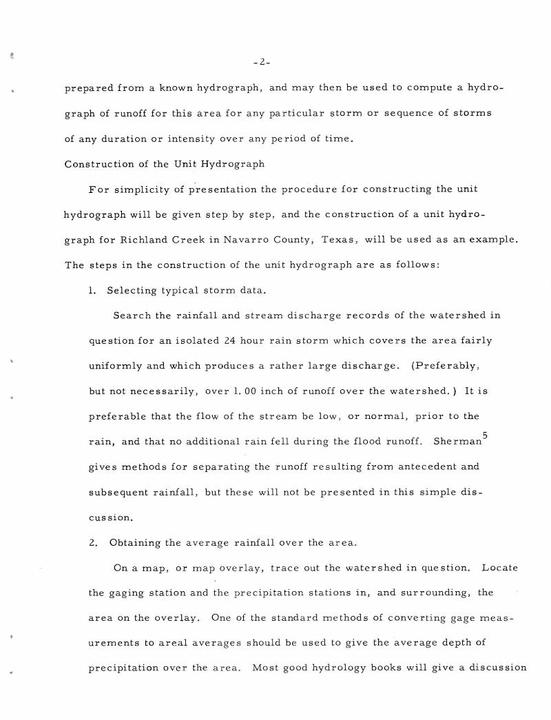
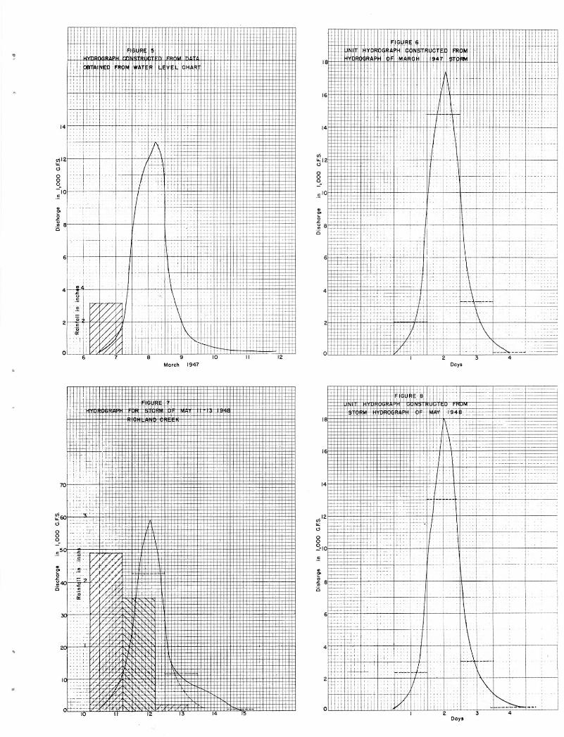
may not, in all cases, be identical with the actual hydrograph. Figure 2
is the hydrograph resulting from a rain storm occurring between late
afternoon of February 17, 1946 and the same time February 18; 1946 on the
Richland Creek watershed. This hydrograph was obtained by the method
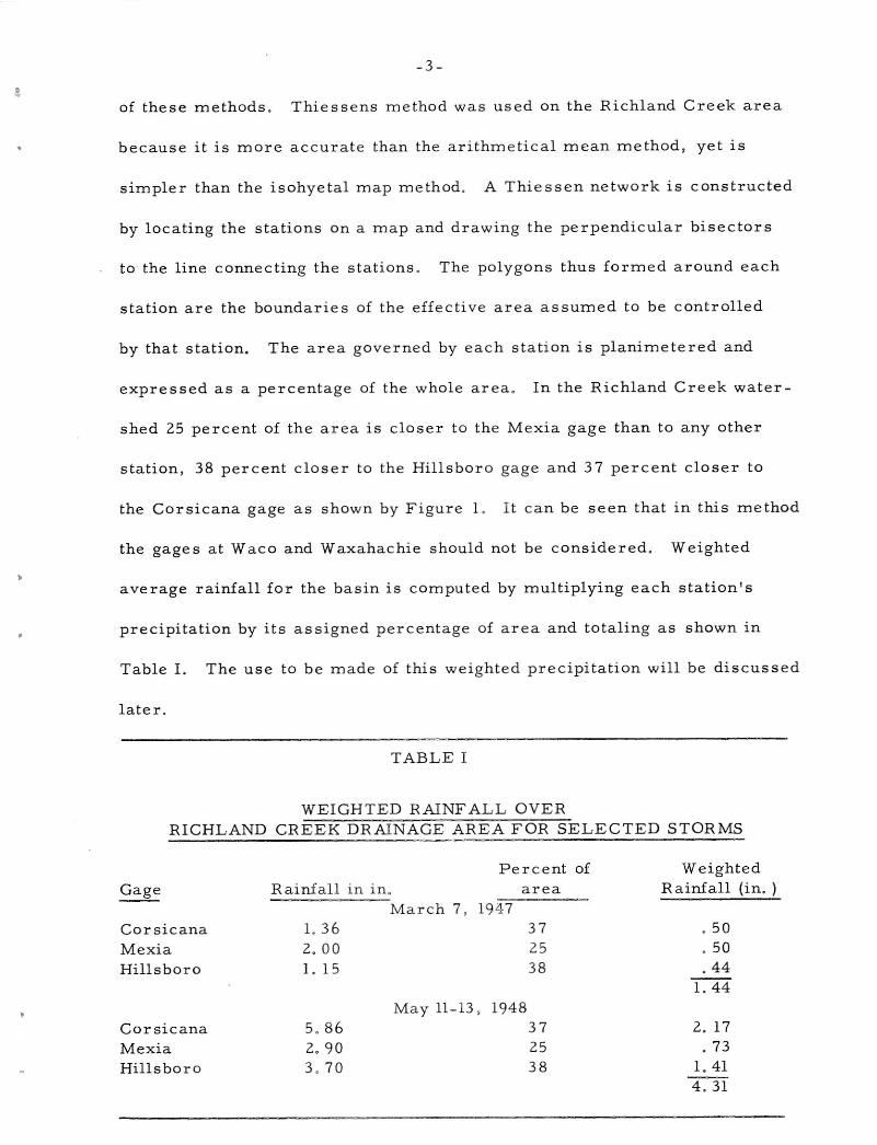
presented above.. Figure 3 is the hydrograph of the same period obtained
from the chart of the water level recorder.
-5-
When the above method is used in plotting the storm hydrograph the
peak obtained may differ materially from the actual peak obtained from
gaging records. This may be noted in Figures 2, 3, 4 and 5. Where the
peak discharge for a given storm is not given in the water supply paper,
it can usually be obtained by writing the U. S. Geological Survey. When
the hydrograph must be plotted without information regarding the peak
flow, the peak discharge for several storms, as given in the water supply
paper, may be compared to their maximum mean daily discharges to obtain
a ratio between the two, which then may be applied to the storm in question.
4. Constructing the unit hydrograph.
The first step in the construction of the unit hydrograph is to separate
the normal or groundwater flow from the total flow. In cases where the
flow was uniform prior to the storm this can be accomplished by drawing
a line across the base of the graph representing this normal flow. All
flow above this line could then be considered as flood flow; In cases where
the flow was affected by an antecedent storm the storm and groundwater
flow can be separated by reproducing across the hydrograph base the
descending leg of the hydrograph from a point equal to the flow just prior
to the storm in question,,
The next step is the determination of the figures for a unit graph for
this drainage area. It will have the same time base as the graph of the
isolated storm in question. The ordinates will be in proportion to the
ordmates of the storm hydrograph as 1, 00 inch is to the depth of runoff
from the area.
-6-
The storm runoff depth is found as follows:
The sum of the average runoff in Column 4 of Table II for period
March 7-10, 1947, is 15, 23 0 second-feet days. This total volume of run
off equals 567 inch miles.
15, 230 sec, ft days X 3600 sec/day X 24 hrs/day X 12 in. /ft 567 m. miles43560 sq, ft. /acre X 640 acres sq. mi.
The total volume of rainfall for this period was 1. 55 in. X 760 sq. mi,
= 1178 in. miles. The percentage of runoff— 567 X 100 — 48.13 percent.1178
The depth of runoff - 1. 55 in. X 48. 13 - .75 in. Column 5 in Table II is
obtained by dividing the values in Column 4 by 0. 75. These values are the
ordinates for the unit graph. The total of Column 5 expressed as inch
miles should equal the drainage area.
It is possible to construct a unit hydrograph from a storm hydrograph
without going through the procedure of weighting the rainfall over the water
shed. In this procedure the depth of runoff over the area is determined
from the volume of storm runoff. If the net runoff of 15, 230 second feet
days, as shown in column 4 of Table II, be converted to depth of runoff
over the 760 square miles of the Richland Creek drainage area, it will
be found to equal , 75 inch which checks with the depth obtained by the other
procedure. The longer procedure of studying the rainfall prior to drawing
the unit graph will allow a more intelligent selection of uniform storms
from which to construct the unit graph.
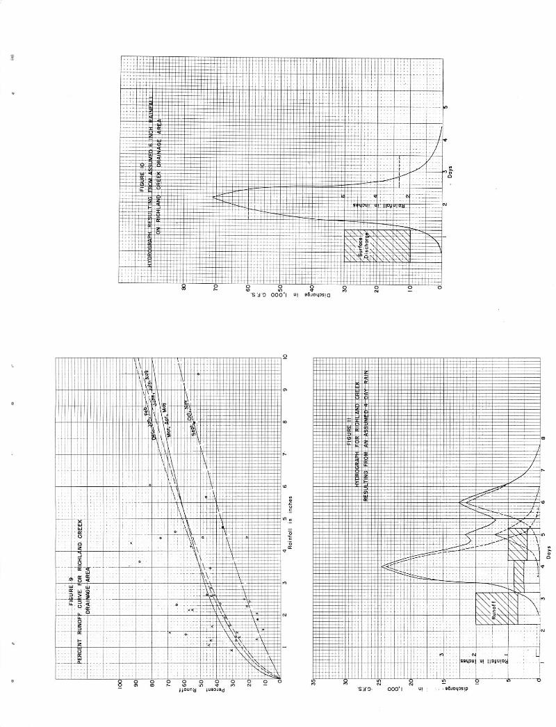
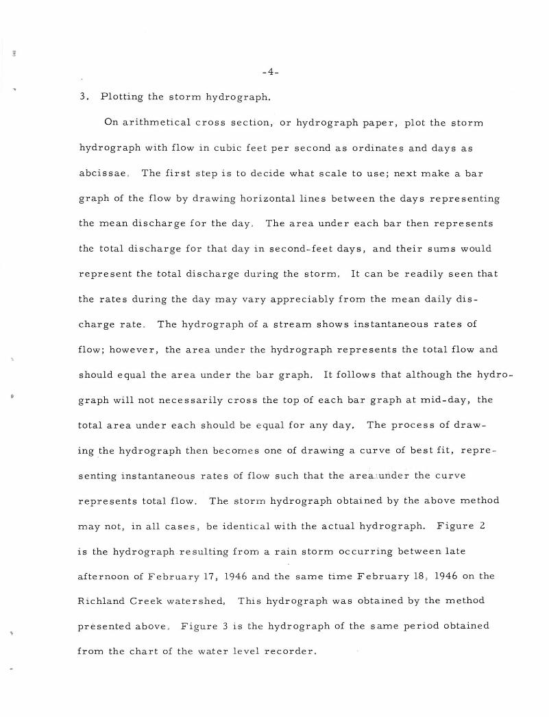
Figure 6 is the unit hydrograph for Richland Creek constructed from
the storm hydrograph of March 6-10, 1947, as shown in Figure 5, As
-7-
mentioned previously this storm hydrograph was plotted from readings
taken off the water level recorder chart. Figure 8 is the unit hydrograph
for this same watershed constructed from the storm hydrograph of May 11-15,
1948. This storm hydrograph was plotted from information as contained in
the U. S. Geological Survey Water Supply Papers; that is, the average daily
flows, and the peak discharge. The receding leg of this hydrograph was
apparently affected by the rainfall on May 13. The runoff for this rainfall
was separated by plotting the normal recession curve for this watershed
as obtained from other hydrographs.
TABLE II
COMPUTATION OF UNIT GRAPHS FOR RICHLAND CREEK
Deduction of
Observed runoff base flow Net runoff Unit graph
Date sec. ft. sec. ft. sec. ft. sec. ft.
March - 1947
6 48 48 ...
7 1600 50 1550 2067
8 112Q0 100 11100 14800
9 2630 150 2480 3307
10 300 200 100 133
11 176 176
Total sec. ft. days 15 230 20307
Total m. miles 567
Total rainfall 1. 44 X 760 = 1094 in. miles
567
1094 = 51. 83 percent runo:iiDepth of runoff • 1. 44 X 51. 83 = .75 in.
May - 194810 24
11 7890
25
50 7840 2676
12 42800 100 42700 14573
13 9000 150 8850 3020
14 600 200 400 137
15 200 200 ___
16 187 187
"59790
...
Total sec. ft. days 20406
Total in. miLes 2224
Total rainfall 4. 3.1 X 760 = 3276
— — 67. 89 percent runoff3 276 - r
Depth of runoff = 4. 31 X 67. 89 = 2. 93
It is to be noted that the two unit graphs thus compare very closely
as to ordinate and base, but there is a small difference in their peaks.
If a number of suitable storm records can be found for the watershed
in question, a unit hydrograph can be prepared from each set of records
and then the peaks of the unit graphs averaged to give the peak of the
3average unit graph. In this regard Linsley, Kohler, and Paulhus state,
"The correct average unit graph should be obtained by locating the aver =
age peak height and time and sketching a mean graph having an area equal
to 1 inch of runoff and resembling the individual graphs as much as possible
It will be noted that the peaks of the various unit graphs will not coincide
nor will the bases be exactly identical." These discrepancies are due in
the main to the inadequacy of the records, which have been mentioned
previously. Rainfall distribution over the watershed will also affect the
detailed shape of the hydrograph.
SYNTHETIC UNIT HYDROGRAPHS
Synthetic unit hydrographs, or hydrographs produced from rainfall and
watershed characteristics rather than from actual stream gaging records,
have two important uses, First, they may be used to check actual unit hydro-
graphs. Second, and most important, the synthetic methods may be applied
to the construction of unit graphs for areas where no gaging records are avail
able,
In synthetic studies, the basic element is the time interval between rain-
7fall and runoff, Snyder has applied the term "lag" to this time interval and
has defined it as the time between center of mass of rainfall excess and the
-9-
resulting peak discharge at the location being studied. In certain other studies,
such as that by Horner and Flynt , there has been used the time interval from
the center of mass of rainfall excess to center of mass of runoff. This has
also been called the "lag. " For this discussion the definition as used by
Snyder will be accepted. The lag for any area may be determined from a study
of rainfall and stream gaging records if such are available; however, in the
procedure to be presented herein it will be assumed that such records are
not available and that the synthetic graph must be derived using only the infor
mation that is to be found on a topographic map,
The following symbols as used by Snyder will be used in this presentation:
t — "Lag" in hoursP 5
t — Unit of duration of surface- runoff producing rain in hours.
t_ — Length of surface runoff producing rain in hours.
T — Time base of unit graph in days.
L = Length of area in miles, measured along the stream.
L„_ = Distance from station on the stream to center of area in miles.C d
A — Effective area contributing to the peak-flow in square miles.
q — Peak-rate of discharge of unit graph in cubic feet per second.
A — Drainage area in square miles.
Ct and C„ — Coefficients depending on units and drainage basin characteristics.
Procedure
1. Determine the center of area of the drainage basin. (A simple method
is to trace the basin outline on stiff paper. Cut it out and suspend it by means
of a string fastened to a pin through a point near the edge and extend the vertical
-10-
line through the area. A line formed by suspending from a second point gives
an intersection, and a third suspension serves as a check. )
Z._ Determine the distance along the stream to the center of area. If the
center of areas is not on the main channel then to a point opposite the center
of area.
3. Determine the length of the stream from the station to its upper end.
0. 34. Determine the lag, by means of formula t = Ct (LcaL) ' , as pro-
5posed by Snyder .
5. By formula qD — C 640/t determine peak flow per square mile of
watershed.
6. Duration of surface runoff is next obtained from the following formula:
T= 3 + 3 (tp/24)
7. A graph is constructed showing the relation of basin-lag and the daily
values of the distribution graph in percent.
8. From the information available a distribution graph and unit hydrograph
are produced.
Example:
The procedure used in developing a synthetic unit graph for Jim Ned Creek
above Colorado Camp dam site in Texas will be given.
From a map of the area the following information was obtained:
L = 52 miles
L__ — 24 miles
0. 3The time lag for the watershed, t — Ct (LcaL) can now be determined
provided a value for C. can be arrived at. Snyder states, "From a study of
-11-
rainfall and gaging records of similar area this value can be determined. " For
the Jim Ned Creek the Corps of Engineers arrived at a value of 1. 0 for this
coefficient. Using this value,
0. 3t _ (1152 X 24)
t — 8, 5 hours (use 9. )
The peak discharge of the unit graph in c. f. s. per square mile is,
qp = Cp 640/tp
For Snyder's studies C ranged from 0. 56 to 0. 69. From the Corps of
Engineers ; studies on Jim Ned Creek it appears that a value of 0. 60 should
be used for C ,
Then,
q - .6 (640)P 9
q _ 42.67 c.f. s. per square mile
The contributing area in this case is 593 sq. miles; therefore,
Q = 42. 67 X 593 - 25,3 03 c.f. s.P
The duration of surface runoff according to Snyder ;s formula is,
T - 3 + 3(9/24)- 4. 125 days
(This value does not check with a unit hydrograph obtained from actual
gaging records on Pecan Bayou, of which Jim Ned Creek is a tributary. The
Pecan Bayou unit graph has a base of 48 hours. )
The time from the beginning of surface runoff to the peak of the unit
graph is equal to t + t /2, and for a 3 hour rain on Jim Ned Creek should be
10. 5 hours.
-12-
There is now available the peak discharge in c.f. s, for the unit graph,
the time from the beginning of surface runoff to the peak in hours, the time
for the base of the hydrograph and the total volume. (1 in runoff from 593 sq.
mi. ) From this information the unit hydrograph curve can be drawn. For
7further refinements in this procedure the reader is referred to Mr, Snyder's
article.
Accuracy of the Method
4Mitchell computed 58 synthetic unit hydrographs for Illinois streams and
checked them against unit graphs computed from actual stream measurements.
He found a probable error of 39. 0 percent in magnitude of crest and 37, 5 percent
in timing.
The accuracy of the synthetic unit hydrograph is dependent to a large
degree on the selection of proper coefficients. These coefficients are arrived
at from consideration of measurements on other watersheds and are in the
main dependent on the judgement and personal opinion of the individual doing
the selecting.
The results obtained by Mitchell are none too good and in the hands of an
inexperienced person the accuracy to be expected would be considerably lessened.
THE USE OF THE UNIT HYDROGRAPH
Constructing a Storm Hydrograph from the Unit Hydrograph
A hydrograph is developed from a unit graph through the following procedure
(a) Daily rainfall properly weighted is listed by date,
(b) A coefficient is applied, reducing rainfall to runoff in inches ofdepth.
-13-
(c) The unit graph value for each day, multiplied bj the runoff depth,gives the increment of stream flow attributable on that day to thedaily rainfall so affected
(d) The horizontal summation of the runoff increments, day by day,produces the total flow and becomes the ordinates of the graph.
This process may be used to
(1) Develop hydrographs for areas where no records are available.These areas should be similar in drainage characteristics andsize to the area from which the unit graph was developed
(2) To develop hydrographs during periods where no records, orincomplete records are available for the watershed in question,
(3) To develop hydrographs for assumed or predicted rain stormsover the subject watershed or similar watershed,
(4) To build a composite unit graph for large areas.
As mentioned above, one of the factors to be considered in developing a
hydrograph from the unit graph is the percentage of runoff to be expected from
the weighted rainfall over the watershed,
Sherman points out that if our consideration be confined to surface runoff
as compared with groundwater subflow seepage, or base flow, we find that the
percentage of runoff increases with the rate and duration of precipitation. The
percentage is also increased by the occurrence of previous precipitations. It
varies with the season according to the temperatures and amount of vegeta
tion, the topography, soil and conditions causing pocket storage and pondage,
Percentages of runoff for different watersheds, or the same watershed,
under varying conditions, may vary greatly, However, if observations are
confined to a sizable area and if they are segregated according to seasons,
5then the data will be quite consistent according to Sherman. If, in addition,

-14 •
the effect of prior precipitation is considered, then the percentage of runoff
will be in harmonious accord. From computations made of percent runoff
of several storms of varying intensity occurring under similar conditions, a
set of curves showing the percent runoff to be expected from storms of vary
ing intensity occurring at different seasons of the year may be drawn, A set
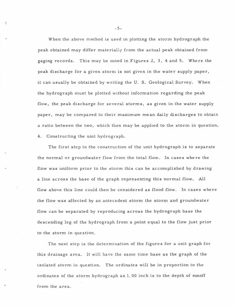
of such curves for Richland Creek is shown in Figure 9
A procedure for estimating the volume of infiltration and surface runoff
has been proposed by Sherman and Mayer , and has been used by Mitchell ,
and others in preference to the percent runoff concept. The procedure as
proposed requires hourly precipitation and runoff records, which are not
always available.
The infiltration approach has not been universally accepted by hydrol-
3ogists. In this regard Linsley, Kohler and Paulhus state as follows:
"Basically the infiltration approach is exceedingly simple, and it is consid
ered by many to be the rational approach. In practical application to natural
drainage basins of sizable proportions, however, so many complications
arise that the procedure is of little value, " These authors further state,
"The infiltration concept can be applied to the rational computation of surface
runoff only when the following factors are essentially uniform throughout the
area under consideration (1) amount, intensity, and duration of rainfall,
(2) infiltration characteristics, (3) surface storage characteristics. These
drastic limitations naturally preclude direct application of the infiltration
approach to any area other than a small plot or experimental basin. "
-15-
It is not the intent in this paper to attempt to discredit either method
but rather to point out that a universally acceptable method for determining
abstractions from precipitation has not been presented at this time.
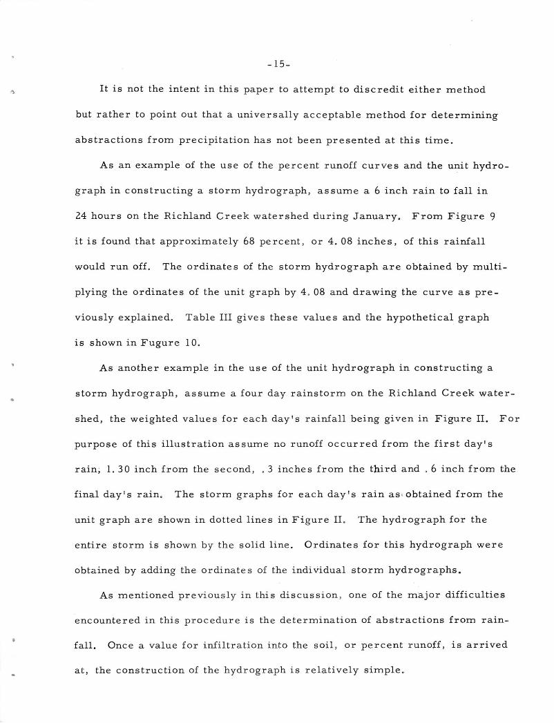
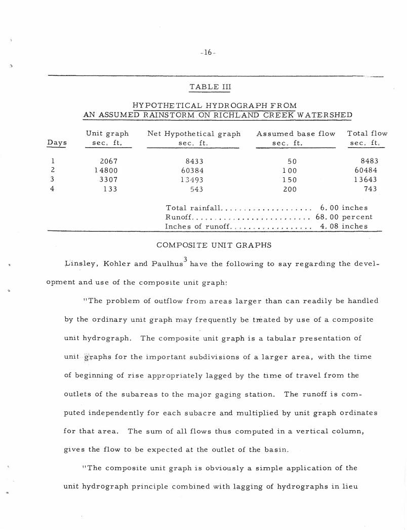
As an example of the use of the percent runoff curves and the unit hydro-
graph in constructing a storm hydrograph, assume a 6 inch rain to fall in
24 hours on the Richland Creek watershed during January. From Figure 9
it is found that approximately 68 percent, or 4. 08 inches, of this rainfall
would run off. The ordinates of the storm hydrograph are obtained by multi
plying the ordinates of the unit graph by 4. 08 and drawing the curve as pre
viously explained. Table III gives these values and the hypothetical graph
is shown in Fugure 10.
As another example in the use of the unit hydrograph in constructing a
storm hydrograph, assume a four day rainstorm on the Richland Creek water
shed, the weighted values for each day's rainfall being given in Figure II. For
purpose of this illustration assume no runoff occurred from the first day's
rain, 1. 30 inch from the second, . 3 inches from the third and . 6 inch from the
final day's rain. The storm graphs for each day's rain as> obtained from the
unit graph are shown in dotted lines in Figure II. The hydrograph for the
entire storm is shown by the solid line. Ordinates for this hydrograph were
obtained by adding the ordinates of the individual storm hydrographs.
As mentioned previously in this discussion, one of the major difficulties
encountered in this procedure is the determination of abstractions from rain
fall. Once a value for infiltration into the soil, or percent runoff, is arrived
at, the construction of the hydrograph is relatively simple.
16
TABLE III
HYPOTHETICAL HYDROGRAPH FROM
AN ASSUMED RAINSTORM ON RICHLAND CREEK WATERSHED
Unit graph Net Hypothetical graph Assumed base flow Total flowDays sec. ft. sec. ft. sec, ft. sec. ft,
1 2067 8433 50 8483
2 14800 60384 100 60484
3 3307 13493 150 13643
4 133 543 200 743
Total rainfall, 6. 00 inches
Runoff. , 68. 00 percent________ Inches of runoff, ..,,.., 4. 08 inches
COMPOSITE UNIT GRAPHS
3Linsley, Kohler and Paulhus have the following to say regarding the devel
opment and use of the composite unit graph:
"The problem of outflow from areas larger than can readily be handled
by the ordinary unit graph may frequently be treated by use of a composite
unit hydrograph. The composite unit graph is a tabular presentation of
unit graphs for the important subdivisions of a larger area, with the time
of beginning of rise appropriately lagged by the time of travel from the
outlets of the subareas to the major gaging station. The runoff is com
puted independently for each subacre and multiplied by unit graph ordinates
for that area. The sum of all flows thus computed in a vertical column,
gives the flow to be expected at the outlet of the basin.
"The composite unit graph is obviously a simple application of the
unit hydrograph principle combined with lagging of hydrographs in lieu
-17-
of routing. It does not account for variations in travel time, which may
be anticipated with widely varying patterns of runoff distribution. Hence
it must be expected to yield only a first approximation to outflow from
areas far greater than those ordinarily treated by the unit graph method.
Its simplicity makes it a useful tool for quick solutions such as may be
required for preliminary design surveys or river forecasting. "
-18-
SUMMARY
Construction of the Unit Hydrograph
The procedure for building a stream hydrograph may be summarized as
follows:
(1) From a study of rainfall and stream gaging records select the
storms to be used
(2) Determine the average depth of precipitation over the area for
the storms selected.
(3) Plot the storm hydrograph.
(4) Separate the normal flow from the flood flow.
(5) Determine the ordinates for the unit graph.
(6) In case more than one storm was selected, average the values
for the peaks of the unit graphs obtained from each storm to obtain
a more accurate unit graph peak for the area.
References Used
1. Corps of Engineers, U. S Army - Report on Pecos Bayou, Texas,
2. Horner, W. W, and Flynt, F L. , Relation Between Rainfall and Runofffrom Small Urban Areas. Trans, American Soc. Civ, Eng. , V. 101,
pp. 140-206. 1936.
3. Linsley, R. K, , Jr., Kohler, M, A., and Paulhus, J. L. H, , AppliedHydrology; McGraw-Hill; New York; 1949..
4. Mitchell, W. D, ; Unit Hydrographs in Illinois, United States Departmentof the Interior and Division of Waterways, State of Illinois; 1948.
5. Sherman, L. K. ; Streamflow from Rainfall by the Unit-graph Method;Eng. News Record; Vol. 108, pp. 501-504, 1932. -----
6. Sherman, L. K. , and Mayer, L. C. , Application of the Infiltration Theoryto Engineering Practice, Trans, American Geophys Union; Part III,pp. 666-77, 1941.
7. Snyder, F. F. ; Synthetic Unit Graphs, Trans. American Geophysical Union;pp. 447-454; 19387
8. Wisler, C. O. , and Brater, E. F. ; Hydrology; John Wiley and Sons, Inc. ;New York; 1949.
Related Documents