The Troublesome Probabilistic Powerdomain

The Troublesome Probabilistic Powerdomain

Achim Jung Regina Tix

Cite as:A. Jung and R. Tix. The troublesome probabilistic powerdomain. In A. Edalat,A. Jung, K. Keimel, and M. Kwiatkowska, editors, Proceedings of the Third Work-shop on Computation and Approximation, volume 13 of Electronic Notes in The-oretical Computer Science. Elsevier Science Publishers B.V., 1998. 23 pages.

Abstract

In [12] it is shown that the probabilistic powerdomain of a continuousdomain is again continuous. The category of continuous domains, however,is not cartesian closed, and one has to look at subcategories such as RB,the retracts of bifinite domains. [8] offers a proof that the probabilisticpowerdomain construction can be restricted to RB.

In this paper, we give a counterexample to Graham’s proof and describeour own attempts at proving a closure result for the probabilistic power-domain construction. We have positive results for finite trees and finitereversed trees. These illustrate the difficulties we face, rather than being asatisfying answer to the question of whether the probabilistic powerdomainand function spaces can be reconciled.

We are more successful with coherent or Lawson-compact domains.These form a category with many pleasing properties but they fall shortof supporting function spaces.

Along the way, we give a new proof of Jones’ Splitting Lemma.

1 Introduction

This paper attempts to highlight one of the unresolved issues in the theory ofthe probabilistic powerdomain. Briefly, the question is whether the probabilisticpowerdomain construction can be defined on a universe of semantic domainswhich is closed under the usual constructions. What we find, in particular, is thatthe probabilistic powerdomain construction is in conflict with function spaces.

The probabilistic powerdomain was first defined by Saheb-Djahromi in 1980,[26]. It has since been studied extensively by Plotkin, Graham, Jones, Kirch,Heckmann and the second author, [25, 8, 13, 12, 21, 9, 10, 28]. Originally, theprobabilistic powerdomain was introduced as a tool in denotational semantics

1

but, more recently, Edalat demonstrated its usefulness in more mainstream math-ematics, most notably in the theory of integration, [2, 4, 3].

From a structural point of view, the probabilistic powerdomain constructionleads to domains with complex internal structure. Topologically, it producescontinuous rather than algebraic domains because of its connection with realnumbers. Order-theoretically, it seems to destroy all lattice-like structure (seeExample 14 below). The first phenomenon is not particularly worrying becausecontinuous domains have been studied alongside algebraic ones since the verybeginning of domain theory, [27, 7, 1]; the second is not new either as the Plotkinpowerdomain construction, [24], has a similar effect.

Considering the use of domains in semantics, one would hope for a “universe”of domains which allows one to perform all kinds of constructions easily and with-out restrictions. Furthermore, one would like these constructions to have good(i.e. meaningful) categorical properties and simple concrete definitions. One wayto go about creating such a semantic universe is to concentrate on the categoricalproperties of the constructions. This is the route taken by axiomatic domaintheory, [6, 5]. The more traditional way is to define constructions concretely andthen prove the categorical properties. The latter approach frequently requiresadditional assumptions about the spaces employed.

Let us illustrate these two alternatives with the probabilistic powerdomainconstruction. While it is true that the probabilistic powerdomain can be definedfor arbitrary dcpo’s (all topological spaces, in fact) and will always yield anotherdcpo, it has been shown to satisfy the axioms for a commutative monad onlyon the much smaller category CONT of continuous domains. If one wants toinsist on the categorical properties for all dcpo’s one must work with an abstractdefinition of a probabilistic powerdomain (for example, as a free probabilisticalgebra), and one loses useful tools and intuitions from measure and integrationtheory.

On the other hand, the concrete approach is not without difficulties either. Infact, the work reported in this paper leads us to believe that some problems maybe insurmountable. These difficulties stem from the fact that CONT as a wholeis not closed under the function space construction. In order to accommodatefunction spaces it is necessary to confine oneself to one of the closed subcategoriesof CONT. These have been completely classified, [15, 1], and the candidate cat-egories in the present setting are RB (also known as RSFP) and FS. The morelattice-like categories such as continuous Scott-domains are unsuitable becausethe probabilistic powerdomain, like the Plotkin powerdomain, destroys existingsuprema. It was claimed in [25, 8] that the probabilistic powerdomain construc-tion applied to an RB-domain yields another RB-domain. The proof offered isnot valid, unfortunately, and whether the statement holds or not is an open ques-tion. We explore this problem in some detail in Section 3, concentrating on theprobabilistic powerdomain of finite posets. Even in this very restricted settingthe problem seems extremely difficult. Our positive results concern trees and re-

2

versed trees but there does not seem to be an easy way to generalize the methodsto all finite posets.

In the last section we explore a more lenient notion of “closed” category,encouraged by our work on relational rather than functional semantics, [16]. Weare able to establish that the probabilistic powerdomain construction behaves wellon Lawson-compact domains. The proof is a bit technical but not too difficult.A more structural proof, preferably applicable to all coherent spaces, would bedesirable.

2 Background

We assume familiarity with the theory of continuous domains as laid out in [1]or [23].

The definition of the probabilistic powerdomain employs the unit intervalI = [0, 1] ⊆ R. We will frequently refer to the order of approximation �I on I,which is characterized simply by a�I b iff a = 0 or a < b.

Definition 1 Let (X, τ) be a topological space. A valuation on X is a functionµ : τ → [0, 1] ⊆ R with the properties

1. µ(∅) = 0;

2. µ(O) + µ(U) = µ(O ∪ U) + µ(O ∩ U), O,U ∈ τ ;

3. O ⊆ U =⇒ µ(O) ≤ µ(U).

In deviation from general practice we will also require a valuation to be Scott-continuous with respect to the Scott-topologies on I and the complete lattice (τ,⊆).

The set of all (continuous) valuations on (X, τ) is called the probabilisticpowerdomain of X. We denote it by PX. On PX one considers the pointwiseordering between valuations

µ ≤ µ′ if µ(O) ≤ µ′(O) for all O ∈ τ .

Valuations have a long history in measure and lattice theory, see [22] andthe references given there. As a construction in denotational semantics, theprobabilistic powerdomain was first defined by Saheb-Djahromi in [26], with theadditional restriction µ(X) = 1. The definition we have chosen is the one of [12].It was later shown by Kirch, [21], that one can extend the range of valuations toR0,+ or even R0,+ ∪ {∞}, retaining the core properties. This extension has theadvantage that we can freely add valuations

(µ+ µ′)(O) = µ(O) + µ′(O)

3

and multiply by non-negative scalars

(r · µ)(O) = r · µ(O) .

PX then becomes an ordered cone. For more details see [28]. For technical reasonswe will stick with Jones’ definition, i.e. we will limit the range of a valuation tothe unit interval.

As every dcpo D is also a topological space when equipped with the Scott-topology σ(D), we can define the probabilistic powerdomain on all dcpo’s. Be-cause addition is a Scott-continuous operation on (R,≤) it follows that PX isagain a dcpo if X = (D, σ(D)). Furthermore, if f : D → E is a Scott-continuousmap between dcpo’s then so is Pf : PD → PE, where

Pf(µ)(O) = µ(f−1(O)), O ∈ σ(E) .

It follows that P is indeed a functor on the category DCPO.Very little is known about the properties of this functor in general. How-

ever, if we restrict its domain of definition to CONT, the category of continuousdomains, then the situation is much better. That is because for continuous do-mains we can make use of so-called simple valuations. In the remainder of thissection we develop the theory of simple valuations in as far as it is relevant forthe purposes of this paper.

Definition 2 A valuation is called simple if it takes on only finitely many dif-ferent values.

Alternatively, simple valuations can be characterised with the help of pointvaluations, as follows.

Proposition 3 Let (X, τ) be a topological space and x ∈ X. Then the followingdefines a valuation ηx on X

ηx(O) =

{1, if x ∈ O;0, otherwise.

We call ηx the point valuation centered at x.

Proposition 4 ([28]) On a sober space X, a valuation µ is simple if and onlyif it is expressible as a linear combination of point evaluations µ =

∑m∈M rmηm,

where M is a finite subset of X.

For a simple valuation µ =∑

m∈M rmηm the measure of an open set O isjust

∑m∈O rm. On a finite poset D equipped with it Scott-topology σ(D), every

valuation is simple since there are only finitely many open sets. If we allow

4

zero weights then we can write every valuation as a linear combination of pointevaluations

µ =∑x∈D

rxηx

with the index set being all points of D. In this case, we can give the followingsimple formula for the weights

rx = µ(↑x)− µ(↑x \ {x}) . (1)

The key result for studying the probabilistic powerdomain construction oncontinuous domains is the so-called Splitting Lemma:

Lemma 5 ([12]) For two simple valuations µ =∑

m∈M rmηm and ν =∑

n∈N rnηnon a continuous domain the following are equivalent

1. µ ≤ ν.

2. There exist non-negative real numbers (tm,n)m∈M,n∈N such that

• ∀m ∈M.∑n∈N

tm,n = rm,

• ∀n ∈ N.∑m∈M

tm,n ≤ rn,

• ∀m ∈M,n ∈ N. If tm,n 6= 0 then m ≤ n.

Throughout this paper, we will call the tm,n appearing in this characterisationthe transport numbers. Although the proof of the Splitting Lemma in [12] is verypretty one may wonder whether there exists a more direct argument. We thereforeinclude the following.

Proof. We show (1) =⇒ (2), which is the difficult direction. Let us call afamily of non-negative real numbers (tm,n)m∈M,n∈N a semi-splitting if the followingis true:

∀m ∈M.∑

n∈N tm,n ≤ rm∀n ∈ N.

∑m∈M tm,n ≤ rn

∀m ∈M,n ∈ N. tm,n 6= 0 =⇒ m ≤ n.

This, of course, is just a slight weakening of the conditions in the statement ofthe lemma.

The set of all semi-splittings is a subset of some Rk (where k = |N | · |M |),which is non-empty (because the null vector belongs to it), closed (because itis defined through inequalities), and bounded (because each tm,n is less than orequal to rn and rm). Therefore this set is compact in the usual metric topologyon Rk.

For a given semi-splitting (tm,n)m∈M,n∈N we call (∑

n∈N tm,n)m∈M the rs-vector(as in row summation). The goal is to show that there exists a semi-splitting

5

whose rs-vector equals (rm)m∈M . Such a semi-splitting would satisfy the condi-tions in (2).

Since the set of all semi-splittings is compact, and since the passage fromsemi-splittings to their rs-vectors is continuous, there exists a semi-splitting withmaximal rs-vector, where “maximal” is taken with respect to the coordinatewiseorder on Rk. We will show that such a semi-splitting is indeed a splitting asrequired.

Assume, for the sake of contradiction, that (tm,n)m∈M,n∈N is a semi-splittingwith maximal rs-vector and that there exists m0 ∈ M with

∑n∈N tm0,n < rm0 .

Define subsets M ′ ⊆M , N ′ ⊆ N inductively by:

1. m0 ∈M ′

2. m ∈M ′,m ≤ n ∈ N =⇒ n ∈ N ′

3. n ∈ N ′, n ≥ m ∈M, tm,n > 0 =⇒ m ∈M ′

Since M and N are finite sets, these subsets are well-defined. Further, let M ′′ =↑M ′ ∩M and O be an open set containing ↑M ′ = ↑M ′′, which does not containany element from either M \M ′′ or N \N ′. We calculate:∑

n∈N ′∑

m∈M tm,n =∑

n∈N ′∑

m∈M ′ tm,n Rule 3=

∑n∈N ′

∑m∈M ′′ tm,n M ′ ⊆M ′′ ⊆M

=∑

m∈M ′′∑

n∈N ′ tm,n<

∑m∈M ′′ rm since m0 ∈M ′′

= (∑

m∈M rmηm)(O) since O ∩M = M ′′

≤ (∑

n∈N rnηn)(O) Assumption=

∑n∈N ′ rn since O ∩N = N ′

Comparing the first and the last term in this chain of inequalities, we observethat there must exist some n ∈ N ′ with

∑m∈M tm,n < rn. Since n belongs to the

inductively defined set N ′, there is a finite chain m0 ≤ no ≥ m1 ≤ n1 ≥ . . . ≤nl = n, pictorially:

m0 m1 m2 ml

n0 n1 n2 nl

On all dotted edges, the transport number tmi+1,niis strictly positive. Therefore,

the following number is also strictly positive:

ε = min {tmi+1,ni| i = 0, . . . , l − 1} ∪ {rn −

∑m∈M

tm,n} ∪ {rm0 −∑n∈N

tm0,n}

6

We define a new semi-splitting by setting

tm,n =

tm,n + ε (m,n) = (mi, ni), i = 0, . . . , l;tm,n − ε (m,n) = (mi+1, ni), i = 0, . . . , l − 1;tm,n otherwise

Pictorially:

m0 m1 m2 ml

n0 n1 n2 nl

ǫ

+ǫ

ǫ ǫ

This adjustment does not change the value of the row summations∑

m∈M tm,ni

for i = 0, . . . , l− 1, and the column summations∑

n∈N tmi,n for i = 1, . . . , l. Thevalues for

∑m∈M tm,nl

and∑

n∈N tm0,n increase by ε each but this is all rightbecause of the second and the third term in the definition of ε. Now observe thatwe have created a semi-splitting (tm,n) whose rs-vector is strictly larger than thatof (tm,n). This contradicts the assumed maximality of the rs-vector for (tm,n) andthe lemma is proven.

Later on we will be concerned with valuations on a fixed finite domain. Forthis case we can formulate the Splitting Lemma even more nicely. Recall thatevery valuation on a finite domain can be written in the form

∑x∈D rxηx with

rx ∈ [0, 1]. The following is then obvious:

Lemma 6 (Elementary Steps) Let D be a finite domain. Consider the fol-lowing relations between valuations on D.

1.∑

x∈D rxηx ≤1

∑x∈D sxηx if there exists x0 ∈ D with rx0 ≤ sx0, and for all

x ∈ D \ {x0}, rx = sx.

2.∑

x∈D rxηx ≤2

∑x∈D sxηx if there exist x0 < x1, where x1 is an upper

neighbour of x0, such that rx1 ≤ sx1 and rx0 + rx1 = sx0 + sx1, and for allx ∈ D \ {x0, x1}, rx = sx.

The order between valuations on D is the transitive hull of ≤1 ∪ ≤2.

In other words, a step of type 1 consists of increasing the mass at some pointof D, and a step of type 2 consists of shifting some mass from a point to one ofits upper neighbours. The lemma states that any two valuations on D, which arecomparable, can be connected by a finite sequence of elementary steps.

Carefully exploiting the information contained in the Splitting Lemma, onecan also give a characterisation of the order of approximation:

7

Lemma 7 ([12]) For two simple valuations µ =∑

m∈M rmηm and ν =∑

n∈N rnηnon a continuous domain the following are equivalent

1. µ� ν.

2. There exist non-negative real numbers (tm,n)m∈M,n∈N such that

• ∀m ∈M.∑n∈N

tm,n = rm,

• ∀n ∈ N.∑m∈M

tm,n �I rn,

• ∀m ∈M,n ∈ N. If tm,n 6= 0 then m� n.

This is instrumental in proving the following:

Theorem 8 ([12]) The probabilistic powerdomain of a continuous domain isagain continuous. A basis is given by the set of simple valuations.

3 The probabilistic powerdomain on cartesian

closed categories

The interpretation of functional types requires a function space construction inthe semantic universe. Since CONT is well pointed there is no choice in thedefinition of a function space; it has to be the set of all continuous functionsordered pointwise. Unfortunately, this dcpo is not continuous in general, see [1,Chapter 4] for a full discussion of this phenomenon. The way out is to considercontinuous domains with additional properties and, indeed, there are a numberof possible definitions. Broadly, these fall into two categories, the lattice-likedomains, where one assumes the existence of certain least upper bounds, andthe compact domains, which are defined with reference to finite posets. ClaireJones demonstrated that lattice-like structure is destroyed by the probabilisticpowerdomain construction in even the simplest cases, so we concentrate attentionon the second kind.

3.1 Trees and RB-domains

Let us first look at retracts of bifinite domains, or RB-domains. We will mostlywork with the following simple internal characterisation of these spaces, [14, The-orem 4.1].

Definition 9 A dcpo D is called an RB-domain if there exists a directed family(fi)i∈I of Scott-continuous functions from D to itself with the following properties.

8

1.∨ ↑

i∈I fi = idD;

2. The image of each fi is finite.

Functions with these properties are called deflations. The full subcategory ofCONT consisting of RB-domains is denoted by RB.

Example 10 Consider the unit interval I = [0, 1] with its usual order. We candefine functions fn : I → I with the desired properties by setting

fn(x) =max {m ∈ N | m�I n · x}

n,

in other words, fn(x) is the largest multiple of 1n

approximating x. (Recall thatr �I s if and only if r = 0 or r < s.)

The function space of two RB-domains is again an object in RB and thereare a number of other pleasing closure properties of this category. The questionthen is whether the probabilistic powerdomain construction can be restricted (or,rather, co-restricted) to RB. This was claimed in [25, 12]. [8] offers a proof butunfortunately it is not valid, and the question in fact remains open.

The problem can easily be reduced to finite posets as follows.

Lemma 11 If it is true that the probabilistic powerdomain of every finite poset isan RB-domain then RB is closed under the probabilistic powerdomain construc-tion.

Proof. Let D be a retract of the bifinite domain E = bilim(Ei) where all Ei arefinite posets. The probabilistic powerdomain functor is locally continuous, hencePD is a retract of PE = bilim(PEi). By assumption, all PEi are RB-domains. Itwas shown in [14, Theorem 4.6] that RB is closed under the formation of bilimits(non-trivial) and retracts (trivial), hence PD belongs to RB.

In order to get the desired closure result one might first try to post-composevaluations directly with the deflations fn : I → I from Example 10. This, how-ever, would destroy modularity.

Since by the previous lemma we can restrict ourselves to finite posets, we canexploit the fact that every valuation on a finite poset D is of the form

∑d∈D rdηd,

with rd ∈ I, ηd the point valuation centered at d ∈ D, and∑

d∈D rd ≤ 1. Ina second attempt we can then apply the deflations fn to weights rather thanvaluations:

Gn : PD → PD, Gn(∑d∈D

rdηd) =∑d∈D

fn(rd)ηd . (2)

This idea is the starting point for the “proof” contained in [8]. While it is truethat each Gn is below idPD and has finite image, and also that

∨ ↑n∈NGn = idPD,

it is unfortunately not the case that they are monotone:

9

Example 12 Consider the two-element chain ⊥ ≤ > and let 0 < ε < 1n< 2ε.

Then 2εη⊥ < εη⊥ + εη> but the images are in reversed order, 1nη⊥ > 0.

What is happening here is that the Gn deal with elementary steps of type 1but not with those of type 2. Our positive result regarding RB concerns finitetrees only; we have not been able to extend it to more general posets.

Theorem 13 The probabilistic powerdomain of a finite tree belongs to RB.

Proof. Every open set in a finite tree is a unique disjoint union of principalfilters (i.e. sets of the form ↑x). We define a deflation on valuations by describingits action on the values for principal filters:

Fn : PD → PD, Fn(µ)(↑x) = fn(µ(↑x)) ,

where the fn are the deflations on I from Example 10. For an arbitrary open setO = ↑y1 ∪ . . . ∪ ↑yk set Fn(µ)(O) =

∑ki=1 fn(µ(↑yi)). We need to show that the

resulting function Fn is a deflation on PD. To this end, we first need to establishthat Fn(µ) is again a valuation on D. Consider first whether Fn(µ) is compatiblewith the relationships between principal filters: if ↑x ⊆ ↑y then µ(↑x) ≤ µ(↑y)and we have Fn(µ)(↑x) ≤ Fn(µ)(↑y) because the fn are monotone.

Next let O be an arbitrary open subset contained in ↑x. Because we areworking on a finite tree, O can be written as a disjoint union ↑y1 ∪ . . .∪ ↑yk. Weneed Fn(µ)(O) ≤ Fn(µ)(↑x) which is equivalent to

∑ki=1 fn(µ(↑yi)) ≤ fn(µ(↑x)).

This relation is a consequence of the super-additivity of the deflations fn:

fn(x) + fn(y) ≤ fn(x+ y)

and the fact that µ itself is a valuation. Now we can apply 1 and recover thepoint masses. This shows that Fn(µ) is indeed a valuation.

So we see that the weight at each node x, calculated as Fn(µ)(↑x)−Fn(µ)(↑x\{x}), is non-negative. Hence Fn(µ) is a valuation.

Monotonicity and continuity of Fn as an operation from PD to PD followfrom the monotonicity and continuity of fn.

Clearly, Fn has finite image because only multiples of 1n

occur as values forFn(µ)(O).

Applying Fn to the valuation ( 1n−ε)η⊥+2εη> on the two-element chain (where

ε < 12n

) we get 1nη⊥. From this we see that the mass assigned to individual points

can be increased by the deflation.An alternative method of proof for the preceding theorem is to establish that

the probabilistic powerdomain of a finite tree is a continuous bounded-completedomain [1, Definition 4.1.1], and to rely on the fact that bc-domains belongto RB. We will not pursue this any further, because the situation for trees isindeed very special in this respect. Already the simplest poset, which is not atree, has a probabilistic powerdomain which is not bounded-complete:

10

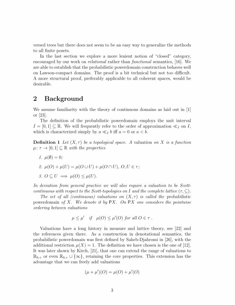
Example 14 ([12]) Consider the poset

c

a b

and the valuations 12ηa and 1

2ηb. They have two distinct minimal upper bounds:

12ηa + 1

2ηb and 1

2ηc.

3.2 Reversed trees and FS-domains

A category related to RB was introduced in [15]. It is also cartesian closed andin fact maximal with this property among the full subcategories of CONT.

Definition 15 A dcpo D is called an FS-domain if there exists a directed family(fi)i∈I of Scott-continuous functions from D to itself with the following properties.

1.∨ ↑

i∈I fi = idD;

2. Every fi is finitely separated from idD in the sense that there exists a finiteset Mi ⊆ D with the property ∀x ∈ D∃m ∈Mi. fi(x) ≤ m ≤ x.

The full subcategory of CONT consisting of FS-domains is denoted by FS.

It is immediate from the definition that every RB-domain belongs to FS aswell. Whether this inclusion is proper is not known.

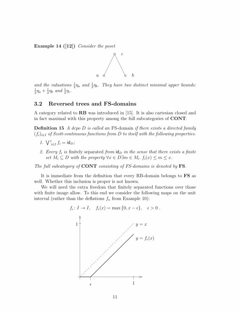
We will need the extra freedom that finitely separated functions over thosewith finite image allow. To this end we consider the following maps on the unitinterval (rather than the deflations fn from Example 10):

fε : I → I, fε(x) = max {0, x− ε}, ε > 0 .

y = x

1

1

ǫ

y = fǫ(x)

11

We shall need some special properties of these functions in our calculations below.

Lemma 16 The functions fε are monotone, Scott-continuous, Hausdorff-contin-uous, and convex. They satisfy the following laws:

a ≤ b =⇒ a− fε(a) ≤ b− fε(b) (3)

a ≤ b, δ ≥ 0 =⇒ fε(b)− fε(a) ≤ fε(b+ δ)− fε(a+ δ) (4)

Each fε is finitely separated from the identity on I. Their supremum equals idI .

Proof. Convexity of functions is equivalent to convexity of the hyper-graph.This is obvious in this case, as are monotonicity and continuity. The two inequal-ities are more interesting:

The first law is proven by a case analysis. If b ≥ a ≥ ε then fε(a) = a− ε andfε(b) = b− ε and both sides of the inequality equal ε. If a < ε ≤ b then fε(a) = 0and fε(b) = b − ε. We get a − fε(a) = a < ε = b − fε(b). Finally, if a ≤ b ≤ εthen both fε(a) and fε(b) equal zero.

The second law is a consequence of convexity. By the convexity property wehave

fε(a+ δ) = fε(b−ab+δ−a · a+ δ

b+δ−a · (b+ δ)) ≤ b−ab+δ−a · fε(a) + δ

b+δ−a · fε(b+ δ)

fε(b) = fε(δ

b+δ−a · a+ b−ab+δ−a · (b+ δ)) ≤ δ

b+δ−a · fε(a) + b−ab+δ−a · fε(b+ δ))

Adding the two inequalities we get

fε(a+ δ) + fε(b) ≤ fε(a) + fε(b+ δ)

from which the desired inequality follows by re-arrangement.As a separating subset for fε one can choose all multiples of ε in I. It is clear

that in the limit we get back idI .

No deflation on I except the constant zero function is convex because convex-ity implies Hausdorff-continuity.

At this point we must confess that we do not have an analogue of Lemma 11for FS-domains. Whether the following results about finite posets will ever beuseful is therefore not at all clear. They do, however, illustrate the technicaldifficulties one faces when trying to establish a general result about the structureof the probabilistic powerdomain construction.

Theorem 17 The probabilistic powerdomain of a finite reversed tree is an FS-domain.

Proof. Since we are working with a reversed tree, every element, except thetop element, has a unique ancestor. Denote the ancestor of x by px. We will needthis (partial) function only to denote open sets of the form ↑px. Setting ↑px = ∅for x = >, the top element, allows us to use a more uniform formalism below.

12

In particular, the translation from values for principal filters to point evaluationstakes the following form. Assume that µ =

∑x∈D rxηx and O ∈ σ(D). Then

µ(O) =∑x∈O

rx =∑x∈O

(µ(↑x)− µ(↑px)

). (5)

Using the functions fε : I → I from above we define a mapping Fε on PD asfollows. For principal filters we set

Fε(µ)(↑x) = fε(µ(↑x)), x ∈ D . (6)

For general open sets O we use the translation from measures for filters to weightson points (Equation 1):

Fε(µ)(O) =∑x∈O

(Fε(µ)(↑x)− Fε(µ)(↑px)

)=

∑x∈O

(fε(µ(↑x))− fε(µ(↑px))

). (7)

The resulting function Fε(µ) is again a valuation, because fε is monotone andso with µ(↑x) ≥ µ(↑px) = µ(↑x \ {x}) we also have Fε(µ)(↑x) = fε(µ(↑x)) ≥fε(µ(↑px)) = Fε(µ)(↑px), that is, the resulting weights are all non-negative.

The crucial part of the proof is in showing that the Fε are monotone. Forthis we need to employ Lemma 6. Assume, therefore, that µ is related to µ′ byan elementary step of type 1, that is, the point mass at some x0 ∈ D is smallerfor µ than it is for µ′ but all other weights are the same. We need to show thatFε(µ)(O) ≤ Fε(µ

′)(O) for all open set O. We will use the definition of Fε(µ)(O)as given in equation 7. To this end we distinguish three kinds of points in D:

Class I consists of those x ∈ D for which x 6≤ x0. Here we have no change inthe measure of principal filters:

fε(µ(↑x))− fε(µ(↑px)) = fε(µ′(↑x))− fε(µ′(↑px))

Class II consists of just x0. Here we have µ(↑x0) ≤ µ′(↑x0) and µ(↑px0) =µ′(↑px0). Hence

fε(µ(↑x0))− fε(µ(↑px0)) ≤ fε(µ′(↑x0))− fε(µ′(↑px0))

Class III contains all elements strictly below x0. This is the trickiest partbecause both ↑x and ↑px are affected by the change at x0. It is here that wemake use of the convexity of fε through rule 4, instantiated as

a := µ(↑px) b := µ(↑x) δ := µ′(↑x)− µ(↑x) = µ′(↑px)− µ(↑px)

13

We getfε(µ(↑x))− fε(µ(↑px)) ≤ fε(µ

′(↑x))− fε(µ′(↑px))

which is the inequality we need. Summing up gives monotonicity for Fε becauseevery x ∈ O belongs to precisely one of the three classes.

Assume now that µ and µ′ are related by an elementary step of type 2, thatis, there exists x0 ∈ D such that some mass has been shifted from x0 to px0 inthe passage from µ to µ′. In order to evaluate equation 7 we again distinguish anumber of cases.

I := {x ∈ D | x 6≤ px0}II := {x ∈ D | x 6≤ x0, x < px0}

III := {x0, px0}IV := {x ∈ D | x < x0}

There is no change in passing from µ to µ′ for elements of class I and IV. The effectfor elements of class II is the same as that for those of class III in the previousparagraph. The two elements in class III need to be considered together.

fε(µ(↑x0))− fε(µ(↑px0)) + fε(µ(↑px0))− fε(µ(↑ppx0)) =

= fε(µ(↑x0))− fε(µ(↑ppx0))= fε(µ

′(↑x0))− fε(µ′(↑ppx0))= fε(µ

′(↑x0))− fε(µ′(↑px0)) + fε(µ′(↑px0))− fε(µ′(↑ppx0))

Summing up over all x gives the desired inequality.Scott-continuity of the Fε follows from the Scott-continuity of the fε.We next show that Fε(µ) ≤ µ holds. To this end we show that the weight at

each point of D is decreased. We use equation 3 from Lemma 16, instantiatedwith b = µ(↑x) and a = µ(↑px):

fε(µ(↑x))− fε(µ(↑px)) ≤ µ(↑x)− µ(↑px)

We also need to check that Fε is finitely separated from the identity on PD.For this we use Graham’s non-monotone (!) functionsGn (Equation 2) with n ∈ Nchosen so that 1

n< ε|D| holds. We prove that for every µ ∈ PD, Fε(µ) ≤ Gε(µ) ≤ µ

holds. Since Gn produces only finitely many different valuations, this will showfinite separation for Fε.

For Fε(µ) ≤ Gε(µ) let O be an open subset of D. We distinguish two cases:either there exists a principal filter ↑X ⊆ O with µ(↑x) ≥ ε or not. In the firstcase, Fε(µ)(O) = fε(µ(↑x)) +

∑y∈O,y 6≥x fε(µ(↑x)) − fε(µ(↑px)) ≤ µ(↑x) − ε +∑

y∈O,y 6≥x µ(↑x) − µ(↑px) where we have used the definition of fε and the factthat Fε reduces the weight at every point. Since Gn can reduce the weight ateach point by at most 1

n< ε|D| , we have Fε(µ) ≤ Gε(µ).

14

In the second case, Fε(µ)(O) = 0 and the desired relationship also holds.The inequality Gn ≤ idPD is trivial.Finally, we want

∨ ↑ε>0 Fε = idPD. This is obvious from the way the Fε are

constructed.

In the proof we have pointed out why it is necessary to have convex approx-imating functions fε on I. There are no convex deflations on I except for theconstant zero map and, indeed, we do not know whether the probabilistic pow-erdomain of a finite reversed tree belongs to RB or not. These spaces, therefore,provide a whole family of domains who may serve as examples that FS is strictlylarger than RB. The only other example is due to Jimmie Lawson; it is describedin [1, p. 60].

4 A positive result for compact domains

If we relax the requirement for function spaces in our universe of semantic do-mains then we get new possibilities. Foremost, there is Jones’ result that theprobabilistic powerdomain construction maps continuous domains to continuousdomains. Topologically, continuous domains are still quite general spaces and itmakes sense to impose further conditions. One of the best known in this con-text is coherence, introduced in [11]. See [1, Section 7.2.4] for an introductionand [23, 18, 19] for some of the many pleasing properties of coherent domains.Recently, it was also shown that these spaces arise quite naturally in a logicalapproach to denotational semantics, [16, 17].

In combination with a continuous dcpo structure, coherence can be charac-terized by Lawson-compactness. We will work with the following criterion forLawson-compactness whose prove is similar to that of Lemma 4.18 in [14]:

Lemma 18 A continuous domain D with bottom element is Lawson-compact, ifand only if, for every situation x � x′, y � y′ there exist finitely many pointsa1, . . . , an in ub{x, y} such that ub{x′, y′} ⊆ ↑{a1, . . . , an}.

Theorem 19 Let D be a Lawson-compact, continuous domain with bottom ele-ment. Then the probabilistic powerdomain is also Lawson-compact.

Proof. We use the characterisation given in Lemma 18 in a slightly sharpenedform by assuming that the two strongly related points are actually taken from abasis. So let µ � µ′ and ν � ν ′ be simple valuations with support M,M ′, N ,and N ′, respectively. We look for finitely many (simple) valuations χ above µand ν, such that every valuation κ above µ′ and ν ′ is above some χ. We may,without loss of generality, assume that κ, too, is simple. In the calculations tofollow it may be helpful to refer to the following picture:

15

m′

m

tm,m′

tm′,k

tm,k

tm,x

x = s(k)

n

n′

k

tx,k

All χ will have the same support X, which we now define. For each pair ofsubsets A′ ⊆M ′, B′ ⊆ N ′ let XA′,B′ be a finite set of upper bounds for ↓↓A′ ∩M ,

↓↓B′ ∩ N which covers ub(A′ ∪ B′). The existence of these sets is guaranteed bythe Lawson-compactness of D (Lemma 18). Let X be the union of all XA′,B′ .

In a first step we will, for a given simple valuation κ above µ′ and ν ′, definea simple valuation χ which is below κ, above µ and ν, and which has its supportin X.

Let such a κ be given. We denote its support by K. The transport numbers,whose existence is guaranteed by the Splitting Lemma, are denoted by tm′,k etc.From the construction of X it then follows that there exists a (not necessarilyinjective) mapping s from K to X with the properties

1. s(k) ≤ k,

2. m� m′ ≤ k =⇒ m ≤ s(k),

3. n� n′ ≤ k =⇒ n ≤ s(k).

Our definition of χ and the corresponding transport numbers are derived fromparticular transport numbers tm,k and tn,k. We calculate these from the transportnumbers corresponding to µ� µ′ ≤ κ as follows:

tm,k :=∑m′∈M ′

tm′,k

rm′tm,m′ and tn,k :=

∑n′∈N ′

tn′,k

rn′tn,n′ .

16

These are valid transport numbers for µ ≤ κ and ν ≤ κ, respectively, since∑k∈K

tm,k =∑k∈K

∑m′∈M ′

tm′,k

rm′tm,m′

=∑m′∈M ′

∑k∈K

tm′,k

rm′tm,m′

=∑m′∈M ′

tm,m′

rm′

∑k∈K

tm′,k

=∑m′∈M ′

tm,m′

rm′rm′

=∑m′∈M ′

tm,m′ = rm

and ∑m∈M

tm,k =∑m∈M

∑m′∈M ′

tm′,k

rm′tm,m′

=∑m′∈M ′

∑m∈M

tm′,k

rm′tm,m′

≤∑m′∈M ′

tm′,k

rm′rm′ ≤ rk

Now we settm,x :=

∑k∈K

s(k)=x

tm,k and tn,x :=∑k∈K

s(k)=x

tn,k .

This definition is necessary because s might not be injective. But s is still afunction, so we retain the properties

rm =∑x∈X

tm,x and rn =∑x∈X

tn,x .

Next we set

ts(k),k := max

{∑m∈M

tm,k,∑n∈N

tn,k

}and for all other x ∈ X we let tx,k := 0. Finally, we can define the weights for χ:

rx :=∑k∈K

tx,k .

Let us now check that χ is indeed above µ and ν and below κ. For this we employthe Splitting Lemma in the reverse direction. We begin with µ ≤ χ: We have

17

already noted that rm =∑

x∈X tm,x. For the inequality we calculate∑m∈M

tm,x =∑m∈M

∑k∈K

s(k)=x

tm,k

=∑k∈K

s(k)=x

∑m∈M

tm,k

≤∑k∈K

s(k)=x

tx,k = rx

The third condition also holds because if tm,x is non-vanishing, then by definitionat least one tm,k with x = s(k) is non-zero. Since we defined tm,k as the sum∑

m′∈M ′tm′,krm′

tm,m′ , at least one termtm′,krm′

tm,m′ is different from zero. This implies

that m� m′ ≤ k holds for this point m′ ∈M ′ and then (2) above yields m ≤ x.Let us now go through the same three steps to show χ ≤ κ. The first condition

holds by definition of the weights of χ. For the second we calculate∑x∈X

tx,k = ts(k),k

=∑n∈N

tn,k (or∑

m∈M tm,k)

≤ rk

The third condition was explicitly enforced.So far, so good. But we get too many valuations χ this way, depending on

how the weight is distributed in the κ’s. We will now show that it is in factpossible to restrict the weights for the valuations χ.

From the relations µ � µ′ and ν � ν ′ we know that∑

m∈M tm,m′ < rm′

and∑

n∈N tn,n′ < rn′ , respectively. As there are just |M ′| + |N ′|-many of thesedifferences we may take their minimum ε1 and set

ε :=ε1

max{|M |, |N |}+ 1.

Consider new valuations µ, ν with weights

rm := rm + ε and rn := rn + ε .

We define transport numbers from µ′ to µ and from ν ′ to ν by setting

tm,m′ :=tm,m′

rmrm and tn,n′ :=

tn,n′

rnrn .

Then µ is still way-below µ′ (and also ν � ν ′):∑m′∈M ′

tm,m′ =∑m′∈M ′

tm,m′

rmrm =

rmrmrm = rm

18

and ∑m∈M

tm,m′ =∑m∈M

tm,m′

rmrm

=∑m∈M

tm,m′

rm(rm + ε)

=∑m∈M

tm,m′ + ε∑m∈M

tm,m′

rm

≤∑m∈M

tm,m′ + ε|M |

<∑m∈M

tm,m′ + ε1 ≤ rm′

For an upper bound κ of µ′ and ν ′ we perform the construction as before, but inthe end we let the weight at each x ∈ X be rx := brxcε, where ε := ε

|X| and brcεis the largest multiple of ε below or equal to r. Because of this alteration, thevaluation χ may no longer be above µ or ν, but it will still be above µ and ν. Forthis we argue from the definition. Let O be a Scott-open set in D which containsat least one element of M (otherwise µ(O) = 0). Then

µ(O) ≤ µ(O)− ε ≤ χ(O)− ε ≤ χ(O) .

There are only finitely many χ if we restrict the maximal weight at each x ∈ Xto be less than or equal to max{µ(D), ν(D)}+ ε1. This completes the proof.

As a concluding remark we observe that this proof is valid independent ofwhether the total mass of valuations is restricted to be 1, to be less than or equalto 1, or whether it is allowed to be any number from the positive extended reals.

5 Open problems

It is annoying and almost embarrassing that we still don’t know whether functionspaces and the probabilistic powerdomain can be reconciled in a category ofcontinuous domains. The question has the irritating feature that it is easier tocome up with a “natural proof” than it is to find the right counterexample. Wehave gone through this iteration a number of times ourselves and our insight intothe problem has not improved much. Theorems 13 and 17 demonstrate that evenfor well-structured posets the formal argument is quite involved.

If we were to suggest further work on the problem then we would probablyrecommend to start with parallel-serial posets. This, however, cannot be thewhole story because we have a proof (not included in this paper) that everyposet of height 2 leads to a probabilistic powerdomain which is FS, and not everysuch poset is parallel-serial.

19

More interesting than a further partial result for finite posets would be ananalogue of Lemma 11 for FS-domains, that is, to show that if the probabilisticpowerdomain of every finite poset is FS then every FS-domain has an FS prob-abilistic powerdomain. Such a proof would almost certainly shed light on otherunresolved issues regarding the category FS.

As indicated at the end of Section 3, the results in this paper provide newexamples of domains which are demonstrably FS but which are not known to bein RB. It would be very nice if we could make further progress on the questionwhether these two categories are different or not.

With respect to the last section it would be quite interesting to see whether aclosure result holds for all coherent spaces, not just the coherent domains. A proofwould have to work quite differently (for example, the topology on PX would notbe the Scott-topology in general) and would most likely be more structural thanthe one offered here.

Acknowledgements

A number of people have been subjected to our (mostly flawed) attempts to provea general closure theorem for the probabilistic powerdomain construction, and wegratefully acknowledge the patience and encouragement of the research teams inDarmstadt and Birmingham.

We would also like to thank two anonymous referees for their comments andMathias Kegelmann for very careful reading and many suggestions for improve-ment.

The result in Section 4 was obtained while the first author visited the IsaacNewton Institute in Cambridge.

References

[1] S. Abramsky and A. Jung. Domain theory. In S. Abramsky, D. M. Gabbay,and T. S. E. Maibaum, editors, Semantic Structures, volume 3 of Handbookof Logic in Computer Science, pages 1–168. Clarendon Press, 1994.

[2] A. Edalat. Dynamical systems, measures and fractals via domain theory:extended abstract. In G. Burn, S. Gay, and M. Ryan, editors, Theory andFormal Methods 1993, Workshops in Computing, pages 82–99. Springer Ver-lag, 1993.

[3] A. Edalat. Domain theory and integration. Theoretical Computer Science,151:163–193, 1995.

[4] A. Edalat. Dynamical systems, measures and fractals via domain theory.Information and Computation, 120(1):32–48, 1995.

20

[5] M. P. Fiore. Axiomatic Domain Theory in Categories of Partial Maps. PhDthesis, University of Edinburgh, 1994. To be published by Cambridge Uni-versity Press in the Distinguished Dissertations Series.

[6] M. P. Fiore, A. Jung, E. Moggi, P. O’Hearn, J. Riecke, G. Rosolini, andI. Stark. Domains and denotational semantics: History, accomplishmentsand open problems. Technical Report CSR-96-2, School of Computer Sci-ence, The University of Birmingham, 1996. 30pp., available from http:-

//www.cs.bham.ac.uk.

[7] G. Gierz, K. H. Hofmann, K. Keimel, J. D. Lawson, M. Mislove, and D. S.Scott. A Compendium of Continuous Lattices. Springer Verlag, 1980.

[8] S. Graham. Closure properties of a probabilistic powerdomain construction.In M. Main, A. Melton, M. Mislove, and D. Schmidt, editors, MathematicalFoundations of Programming Language Semantics, volume 298 of LectureNotes in Computer Science, pages 213–233. Springer Verlag, 1988.

[9] R. Heckmann. Probabilistic power domains, information systems, and lo-cales. In S. Brookes, M. Main, A. Melton, M. Mislove, and D. Schmidt,editors, Mathematical Foundations of Programming Semantics VIII, volume802 of Lecture Notes in Computer Science, pages 410–437. Springer Verlag,1994.

[10] R. Heckmann. Spaces of valuations. In S. Andima, R. C. Flagg, G. Itzkowitz,P. Misra, Y. Kong, and R. Kopperman, editors, Papers on General Topologyand Applications: Eleventh Summer Conference at the University of South-ern Maine, volume 806 of Annals of the New York Academy of Sciences,pages 174–200, 1996.

[11] K. H. Hofmann and M. Mislove. Local compactness and continuous lattices.In B. Banaschewski and R.-E. Hoffmann, editors, Continuous Lattices, Pro-ceedings Bremen 1979, volume 871 of Lecture Notes in Mathematics, pages209–248. Springer Verlag, 1981.

[12] C. Jones. Probabilistic Non-Determinism. PhD thesis, University of Edin-burgh, Edinburgh, 1990. Also published as Technical Report No. CST-63-90.

[13] C. Jones and G. Plotkin. A probabilistic powerdomain of evaluations. InProceedings of the 4th Annual Symposium on Logic in Computer Science,pages 186–195. IEEE Computer Society Press, 1989.

[14] A. Jung. Cartesian Closed Categories of Domains, volume 66 of CWI Tracts.Centrum voor Wiskunde en Informatica, Amsterdam, 1989. 107 pp.

21

[15] A. Jung. The classification of continuous domains. In Proceedings, FifthAnnual IEEE Symposium on Logic in Computer Science, pages 35–40. IEEEComputer Society Press, 1990.

[16] A. Jung, M. Kegelmann, and M. A. Moshier. Multi lingual sequent calculusand coherent spaces. In S. Brookes and M. Mislove, editors, 13th Conferenceon Mathematical Foundations of Programming Semantics, volume 6 of Elec-tronic Notes in Theoretical Computer Science. Elsevier Science PublishersB.V., 1997. 18 pages.

[17] A. Jung, M. Kegelmann, and M. A. Moshier. Multi lingual sequent calcu-lus and coherent spaces. Technical Report CSR-97-9, School of ComputerScience, The University of Birmingham, 1997. 41 pages, (submitted forpublication).

[18] A. Jung and Ph. Sunderhauf. On the duality of compact vs. open. InS. Andima, R. C. Flagg, G. Itzkowitz, P. Misra, Y. Kong, and R. Kopperman,editors, Papers on General Topology and Applications: Eleventh SummerConference at the University of Southern Maine, volume 806 of Annals ofthe New York Academy of Sciences, pages 214–230, 1996.

[19] A. Jung and Ph. Sunderhauf. Uniform approximation of topological spaces.Topology and its Applications, 83(1):23–38, 1998.

[20] A. Jung and R. Tix. The troublesome probabilistic powerdomain. InA. Edalat, A. Jung, K. Keimel, and M. Kwiatkowska, editors, Proceedingsof the Third Workshop on Computation and Approximation, volume 13 ofElectronic Notes in Theoretical Computer Science. Elsevier Science Publish-ers B.V., 1998. 23 pages.

[21] O. Kirch. Bereiche und Bewertungen. Master’s thesis, Technische HochschuleDarmstadt, June 1993. 77pp.

[22] J. D. Lawson. Valuations on continuous lattices. In Rudolf-Eberhard Hoff-mann, editor, Continuous Lattices and Related Topics, volume 27 of Mathe-matik Arbeitspapiere, pages 204–225. Universitat Bremen, 1982.

[23] J. D. Lawson. The versatile continuous order. In M. Main, A. Melton,M. Mislove, and D. Schmidt, editors, Mathematical Foundations of Pro-gramming Language Semantics, volume 298 of Lecture Notes in ComputerScience, pages 134–160. Springer Verlag, 1988.

[24] G. D. Plotkin. A powerdomain construction. SIAM Journal on Computing,5:452–487, 1976.

22

[25] G. D. Plotkin. Probabilistic powerdomains. In Proceedings CAAP, pages271–287, 1982.

[26] N. Saheb-Djahromi. CPO’s of measures for nondeterminism. TheoreticalComputer Science, 12:19–37, 1980.

[27] D. S. Scott. Continuous lattices. In E. Lawvere, editor, Toposes, AlgebraicGeometry and Logic, volume 274 of Lecture Notes in Mathematics, pages97–136. Springer Verlag, 1972.

[28] R. Tix. Stetige Bewertungen auf topologischen Raumen. Master’s thesis,Technische Hochschule Darmstadt, June 1995. 51pp.

Achim JungSchool of Computer ScienceThe University of BirminghamEdgbastonBirmingham, B15 [email protected]

Regina TixFachbereich MathematikTechnische Universitat DarmstadtD–64289 [email protected]

23