The trouble with H0 - arXiv

Prepared for submission to JCAP

The trouble with H0

Jose Luis Bernala,b Licia Verdea,c,d,e,f Adam G. Riessg,h

aICC, University of Barcelona, IEEC-UB, Martı i Franques, 1, E08028 Barcelona, SpainbDept. de Fısica Quantica i Astrofısica, Universitat de Barcelona, Martı i Franques 1, E08028Barcelona, SpaincICREA, Pg. Lluıs Companys 23, 08010 Barcelona, SpaindRadcliffe Institute for Advanced Study, Harvard University, MA 02138, USAf Institute for Theory and Computation, Harvard-Smithsonian Center for Astrophysics, 60 GardenStreet, Cambridge, MA 02138, USAeInstitute of Theoretical Astrophysics, University of Oslo, 0315, Oslo, NorwaygDepartment of Physics and Astronomy, Johns Hopkins University, Baltimore, MD 21218hSpace Telescope Science Institute, 3700 San Martin Drive, Baltimore, MD 21218

E-mail: [email protected], [email protected], [email protected]

Abstract. We perform a comprehensive cosmological study of the H0 tension between the directlocal measurement and the model-dependent value inferred from the Cosmic Microwave Background.With the recent measurement of H0 this tension has raised to more than 3σ. We consider changes inthe early time physics without modifying the late time cosmology. We also reconstruct the late timeexpansion history in a model independent way with minimal assumptions using distance measurementsfrom Baryon Acoustic Oscillations and Type Ia Supernovae, finding that at z < 0.6 the recoveredshape of the expansion history is less than 5% different than that of a standard ΛCDM model. Theseprobes also provide a model insensitive constraint on the low-redshift standard ruler, measuringdirectly the combination rsh where H0 = h×100 Mpc−1km/s and rs is the sound horizon at radiationdrag (the standard ruler), traditionally constrained by CMB observations. Thus rs and H0 provideabsolute scales for distance measurements (anchors) at opposite ends of the observable Universe. Wecalibrate the cosmic distance ladder and obtain a model-independent determination of the standardruler for acoustic scale, rs. The tension in H0 reflects a mismatch between our determination ofrs and its standard, CMB-inferred value. Without including high-` Planck CMB polarization data(i.e., only considering the “recommended baseline” low-` polarisation and temperature and the high `temperature data), a modification of the early-time physics to include a component of dark radiationwith an effective number of species around 0.4 would reconcile the CMB-inferred constraints, and thelocal H0 and standard ruler determinations. The inclusion of the “preliminary” high-` Planck CMBpolarisation data disfavours this solution.

arX

iv:1

607.

0561

7v2

[as

tro-

ph.C

O]

20

Oct

201

6

Contents

1 Introduction 1

2 Data 3

3 Methods 4

4 Modifying early Universe physics: effect on H0 and rs 6

5 Changing late-time cosmology 95.1 Reconstruction independent from the early-time physics 13

6 Discussion and Conclusions 17

1 Introduction

In the last few years, the determination of cosmological parameters has reached astonishing andunprecedented precision. Within the standard Λ - Cold Dark Matter (ΛCDM) cosmological modelsome parameters are constrained at or below the percent level. This model assumes a spatially flatcosmology and matter content dominated by cold dark matter but with total matter energy densitydominated by a cosmological constant, which drives a late time accelerated expansion. Such precisionhas been driven by a major observational effort. This is especially true in the case of Cosmic MicrowaveBackground (CMB) experiments, where WMAP [1, 2] and Planck [3] have played a key role, but alsoin the measurements of Baryon Acoustic Oscillations (BAO) [4, 5], where the evolution of the cosmicdistance scale is now measured with a ∼ 1% uncertainty.

The Planck Collaboration 2015 [3] presents the strongest constraints so far in key parameters,such as geometry, the predicted Hubble constant, H0, and the sound horizon at radiation drag epoch,rs. These last two quantities provide an absolute scale for distance measurements at opposite ends ofthe observable Universe (see e.g., [6, 7]), which makes them essential to build the distance ladder andmodel the expansion history of the Universe. However, they are indirect measurements and as suchthey are model-dependent. Whereas the H0 constraint assumes an expansion history model (whichheavily relies on late time physics assumptions such as the details of late-time cosmic acceleration,or equivalently, the properties of dark energy), rs is a derived parameter which relies on early timephysics (such as the density and equation of state parameters of the different species in the earlyuniverse).

This is why having model-independent, direct measurements of these same quantities is of utmostimportance. In the absence of significant systematic errors, if the standard cosmological model isthe correct model, indirect (model-dependent) and direct (model-independent) constraints on theseparameters should agree. If they are significantly inconsistent, this will provide evidence of physicsbeyond the standard model (or unaccounted systematic errors).

Direct measurements of H0 rely on the ability to measure absolute distances to > 100 Mpc, usu-ally through the use of coincident geometric and relative distance indicators. H0 can be interpreted asthe normalization of the Hubble parameter, H(z), which describes the expansion rate of the Universeas function of redshift. Previous constraints on H0 (i.e. [8]) are consistent with the final results fromthe WMAP mission, but are in 2-2.5σ tensions with Planck when ΛCDM model is assumed [9–11].The low value of H0 found, within the ΛCDM model, by the Planck Collaboration since its first datarelease [12], and confirmed by the latest data release [3], has attracted a lot of attention. Re-analysesof the direct measurements of H0 have been performed ([13] including the recalibration of distances of[14]); physics beyond the standard model has been advocated to alleviate the tension, especially highernumber of effective relativistic species, dynamical dark energy and non-zero curvature [7, 15–19].

– 1 –

In some of these model extensions, by allowing the extra parameter to vary, tension is reduced butthis is mainly due to weaker constraints on H0 (because of the increased number of model parameters),rather than an actual shift in the central value. In many cases, non-standard values of the extraparameter appear disfavoured by other data sets.

Recent improvements in the process of measuring H0 (an increase in the number of SNeIa cal-ibrated by Cepheids from 8 to 19, new parallax measurements, stronger constraints on the Hubbleflow and a refined computation of distance to NGC4258 from maser data) have made possible a 2.4%measurement of H0: H0 = 73.24 ± 1.74 Mpc−1km/s [20]. This new measurement increases the ten-sion with respect to the latest Planck-inferred value [21] to ∼ 3.4σ. This calibration of H0 has beensuccessfully tested with recent Gaia DR1 parallax measurements of cepheids in [22].

Time-delay cosmography measurements of quasars which pass through strong lenses is anotherway to set independent constraints on H0. Effort in this direction is represented by the H0LiCOWproject [23]. Using three strong lenses, they find H0 = 71.9+2.4

−3.0 Mpc−1km/s, within flat ΛCDM withfree matter and energy density [24]. Fixing ΩM = 0.32 (motivated by the Planck results [3]), yieldsa value H0 = 72.8± 2.4 Mpc−1km/s. These results are in 1.7σ and 2.5σ tension with respect to themost-recent CMB inferred value, while are perfectly consistent with the local measurement of [20].

In addition, in [25], it is shown that the value of H0 depends strongly on the CMB multipolerange analysed. Analysing only temperature power spectrum, tension of 2.3σ between the H0 from` < 1000 and from ` ≥ 1000 is found, the former being consistent with the direct measurement of[20]. However, Ref. [26] finds that the shifts in the cosmological parameters values inferred from lowversus high multipoles are not highly improbable in a ΛCDM model (consistent with the expectationswithin a 10%). These shifts appear because when considering only multipoles ` < 800 (approximatelythe range explored by WMAP) the cosmological parameters are more strongly affected by the wellknown ` < 10 power deficit.

Explanation for this tension in H0 includes internal inconsistencies in Planck data systematicsin the local determination of H0 or physics beyond the standard model. These recent results clearlymotivate a detailed study of possible extensions of the ΛCDM model and an inspection of the currentcosmological data sets, checking for inconsistencies.

In figure 1, we summarize the current constraints on H0 tied to the CMB and low-redshift mea-surements. We show results from the public posterior samples provided by the Planck Collaboration2015 [3], WMAP9 [1] (analysed with the same assumptions of Planck)1, the results of the work ofAddison et al. [25] and the quasar time-delay cosmography measurements of H0 [24], along with thelocal measurement of [20]. CMB constraints are shown for two models: a standard flat ΛCDM anda model where the effective number of relativistic species Neff is varied in addition to the standardΛCDM parameters. Of all the popular ΛCDM model extensions, this is the most promising one toreduce the tension. Assuming ΛCDM, the CMB-inferred H0 is consistent with the local measurementonly when ` < 1000 are considered (the work of Addison et al. and WMAP9). However when BAOmeasurements are added to WMAP9 data, the tension reappears, but at a lower level (2.8σ).

On the other hand, rs is the standard ruler which calibrates the distance scale measurementsof BAO. Since BAO measure DV /rs (or DA/rs and Hrs in the anisotropic analysis) the only wayto constrain rs without making assumptions about the early universe physics is combining the BAOmeasurement with other probes of the expansion rate (such as H0, cosmic clocks [29] or gravitationallensing time delays [23]). When no cosmological model is assumed, H0 and rs are understood asanchors of the cosmic distance ladder and the inverse cosmic distance ladder, respectively. As BAOmeasurements always depends on the product H0rs (see Equations (5.1), (5.2) and (5.3)), when theUniverse expansion history is probed by BAO, the two anchors are related by H0rs = constant. Thiswas illustrated in [30] and more recently in [31], where only weak assumptions are made on the shapeof H(z), and in [6], where the normal and inverse distance ladder are studied in the context of ΛCDMand typical extensions.

1The values of rs in WMAP’s public posterior samples were computed using the approximation of [27], which differsfrom the values computed by current Boltzmann codes and used in Planck’s analysis by several percent, as pointed inthe appendix B of Ref. [28]. As WMAP’s data have been re-analysed by the Planck Collaboration, the values reportedhere are all computed with the same definition.

– 2 –

60 65 70 75 80

H0 (Mpc−1 km/s)

0

5

10

15

20

25

30

WMAP9

WMAP9+BAO

P15 (TT)

P15 (T+P)

P15 (T+P)+lensing

P15 (T+P)+BAO

P15 (T+P)+lensing+ext

P15 (TT) `<1000

P15 (TT) `≥1000

H0LiCOW

H0LiCOW +ΩM prior

P15 (TT)

P15 (T+P)

P15 (T+P)+lensing

P15 (T+P)+BAO

P15 (T+P)+lensing+ext

(1.3σ)

(2.8σ)

(3.2σ)

(3.4σ)

(3.1σ)

(3.2σ)

(3.0σ)

(1.5σ)

(3.8σ)

(0.4σ)

(0.2σ)

(1.7σ)

(2.7σ)

(2.8σ)

(2.7σ)

(2.6σ)

CMB ΛCDM+Neff

H0LiCOW

CMB ΛCDM

R16

Figure 1. Marginalised 68% and 95% constraints on H0 from different analysis of CMB data, obtained from PlanckCollaboration 2015 public chains [3], WMAP9 [1] (analysed with the same assumptions than Planck) and the results ofthe work of Addison et al. [25] and Bonvin et al. [24]. We show the constraints obtained in a ΛCDM context in blue,ΛCDM+Neff in red, quasar time-delay cosmography results (taken from H0LiCOW project [24], for a ΛCDM model,with and without relying on a CMB prior for ΩM) in green and the constraints of the independent direct measurementof [20] in black. We report in parenthesis the tension with respect to the direct measurement.

While the model-independent measurement of rs [30] is consistent with Planck, the model-dependent value of [6] is in 2σ tension with it. Both of these measurements use H0 ≈ 73.0 ±2.4Mpc−1km/s, so, this modest tension is expected to increase with the new constraint on H0.

In this paper we quantify the tension in H0 and explore how it could be resolved –withoutinvoking systematic errors in the measurements– by studying separately changes in the early timephysics and in the late time physics

We follow three avenues. Firstly, we allow the early cosmology (probed mostly by the CMB)to deviate from the standard ΛCDM assumptions, leaving unaltered the late cosmology (e.g., theexpansion history at redshift below z ∼ 1000 is given by the ΛCDM model). Secondly, we allowfor changes in the late time cosmology, in particular in the expansion history at z ≤ 1.3, assumingstandard early cosmology (i.e., physics is standard until recombination, but the expansion history atlate time is allowed to be non-standard). Finally, we reconstruct in a model-independent way, the late-time expansion history without making any assumption about the early-time physics, besides assumingthat the BAO scale corresponds to a standard ruler (with unknown length). By combining BAO withSNeIa and H0 measurements we are able to measure the standard ruler in a model-independent way.Comparison with the Planck-derived determination of the sound horizon at radiation drag allows usto assess the consistency of the two measurements within the assumed cosmological model.

In section 2 we present the data sets used in this work and in section 3 we describe the methodol-ogy. We explore modifications of early-time physics from the standard ΛCDM (leaving unaltered thelate-time ones) in section 4 while changes in the late-time cosmology are explored in section 5. Herewe present the findings both assuming standard early-time physics and in a way that is independentfrom it. Finally we summarize the conclusions of this work in section 6.

2 Data

The observational data we consider are: measurements of the Cosmic Microwave Background (CMB),Baryon Acoustic Oscillations (BAO), Type Ia Supernovae (SNeIa) and direct measurements of theHubble constant H0.

– 3 –

We consider the full Planck 2015 temperature (TT), polarization (EE) and the cross correlationof temperature and polarization (TE) angular data [3], corresponding to the following likelihoods:Planck high ` (30 ≤ ` ≤ 2508) TTTEEE for TT (high ` TT), EE and TE (high ` TEEE) and thePlanck low` for TT, EE, TE and BB (lowP, 2 ≤ ` ≤ 29). The Planck team [3, 32] identifies thelowP + high ` TT as the “recommended baseline” dataset and the high ` polarisation (high ` TEEE)as “preliminary”, because of evidence of low level systematics (∼ (µK)2 in `(` + 1)C`). While thelevel of systematic contamination does not appear to affect parameter estimation, we neverthelesspresent results both excluding and including the high ` polarisation data. In addition, we use thelensing reconstruction signal for the range 40 ≤ L ≤ 400, which we refer to as CMB lensing. For somemodels we use the publicly available posterior samples (i.e., public chains) provided by the Planckcollaboration: ΛCDM, ΛCDM+Neff (a base ΛCDM model with an extra parameter for the effectivenumber of neutrino species) and ΛCDM +Y BBN

P (a base ΛCDM model with an extra parameter forthe primordial Helium abundance). In addition, we use the analysis of WMAP9 data with the sameassumptions of Planck, which is publicly available along with the rest of Planck data. We also usethe results of Addison et al. [25], where the Planck’s temperature power spectrum is analysed in twoseparate multipole ranges: ` < 1000 and ` ≥ 1000.

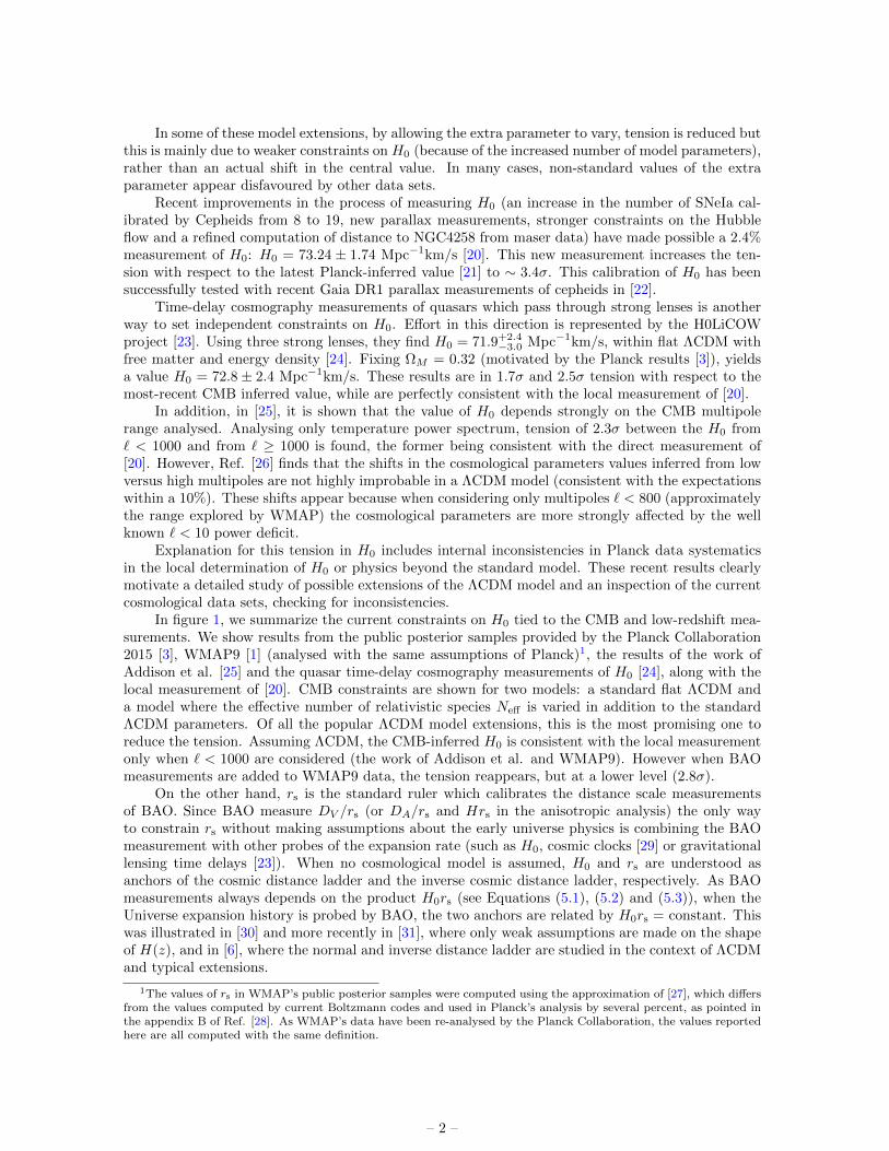
We use constraints on BAO from the following galaxy surveys: Six Degree Field Galaxy Survey(6dF) [33], the Main Galaxy Sample of Data Release 7 of Sloan Digital Sky Survey (SDSS-MGS)[34], the LOWZ and CMASS galaxy samples of the Baryon Oscillation Spectroscopic Survey (BOSS-LOWZ and BOSS-CMASS, respectively) [5], and the reanalysed measurements of WiggleZ [35]. Thesemeasurements, and their corresponding effective redshift zeff , are summarized in table 1. Note that forBOSS-CMASS there is an isotropic measurement (DV /rs) and an anisotropic measurement (DA/rs,Hrs), which, of course, we never combine. When we use the anisotropic values from BOSS-CMASSin section 4, we take into account that they are correlated (their correlation coefficient is 0.55). Weuse the covariance matrix for the measurements of WiggleZ as indicated in Ref. [35]. We considerthat the measurements of BOSS-CMASS and WiggleZ are independent, although the regions coveredby both surveys overlap. We can do so because this overlap includes a small fraction of the BOSS-CMASS sample and the correlation is very small too (always below 4%) [5, 36], hence the constraintswhich come from both surveys are fairly independent. The BOSS collaboration also provides a BAOmeasurement at z ∼ 2.5 obtained from Lymanα forest observed in Quasars spectra. We do not includethis measurement because, as it will be clear later, our approach relies on having BAO and SNeIa datacovering roughly the same redshift range. Considering an extra BAO point at high redshift wouldhave increased the number of parameters needed to describe the expansion history without improvingconstraints in any of the quantities we are interested in.

The publicly available Planck 2015 posterior sampling uses a slightly different BAO data set (seeRef. [3] for details). However the small difference in the data set does not drive any significant effectin the parameter constraints.

For SNeIa cosmological observations, we use the SDSS-II/SNLS3 Joint Light-curve Analysis(JLA) data compilation [37]. This catalog contains 740 spectroscopically confirmed SNeIa obtainedfrom low redshift samples (z < 0.1), all three seasons of the Sky Digital Sky Survey II (SDSS-II)(0.05 < z < 0.4) and the three years of the SuperNovae Legacy Survey (SNLS) (0.2 < z < 1) togetherwith nine additional SNeIa at high redshift from HST (0.8 < z < 1.3). We use the compressed formof the JLA likelihood (Appendix E of Ref. [37]).

Finally, we use the distance recalibrated direct measurement of H0 from [20], which is H0 =73.24± 1.74 Mpc−1km/s.

3 Methods

We use the public Boltzmann code CLASS [38, 39] and the Monte Carlo public code Monte Python[40] to analyse the CMB data sets discussed in section 2 when for the selected model there are noposterior samples officially provided by the Planck collaboration. We modify the codes to include theparametrized extra dark radiation, ∆Neff and the effective parameters to describe its behaviour, c2s

– 4 –

Survey zeff Parameter Measurement

6dF [33] 0.106 rs/DV 0.327± 0.015

SDSS-MGS [34] 0.15 DV /rs 4.47± 0.16

BOSS-LOWZ [5] 0.32 DV /rs 8.59± 0.15

WiggleZ [35] 0.44 DV /rs 11.6± 0.6

BOSS-CMASS [5] 0.57 DV /rs 13.79± 0.14

BOSS-CMASS [5] 0.57 DA/rs 9.52± 0.14

BOSS-CMASS [5] 0.57 Hrs 14750± 540

WiggleZ [35] 0.6 DV /rs 15.0± 0.7

WiggleZ [35] 0.73 DV /rs 16.9± 0.6

Table 1. BAO data measurements included in our analysis, specifying the survey that obtained each measurementand the corresponding effective redshift zeff . In the case where we change the late time cosmology, we use the isotropicmeasurements. We take into account the correlation between the anisotropic measurements of BOSS-CMASS andamong the values from WiggleZ.

and c2vis (section 4) additional parameters to the Planck “base” model 2 . We adopt uniform priors forall the parameters, except for ∆Neff , for which we sample ∆N2

eff (see section 4). We only set a lowerlimit in the sampling range for As, ns, τ and ∆Neff (0.0 in all cases but for τ , which is 0.04). Theprior in τ has virtually no effect on the reported constraints and is justified by observations of theGunn–Peterson effect, see e.g., Ref. [41]. Our sampling method of choice when CMB data are involvedis the Metropolis Hastings algorithm; we run sixteen Monte Carlo Markov Chains (MCMC) for eachensemble of data sets until the fundamental parameters reach a convergence parameter R− 1 < 0.03,according to the Gelman-Rubin criterion [42].

When interpreting the low redshift probes of the expansion history (see section 5), we use adifferent methodology. We aim to reconstruct H(z) (the main observable related with the expansionof the Universe) in the most model-independent way possible, but still requiring a smooth expansionhistory. For this reason the Hubble function is expressed as piece-wise natural cubic splines in theredshift range 0 ≤ z ≤ 1.3. We specify the spline function Hrecon(z) by the values it takes at N“knots” in redshift. These values uniquely define the piecewise cubic spline once we ask for continuityof Hrecon(z) and its first and second derivatives at the knots, and two boundary conditions. Werequire the second derivative to vanish at the exterior knots. Thus, our free parameters are the valuesof Hrecon(zknot), where zknot are the redshifts correspondent to the “knots”. We also consider cases inwhich we vary the sound horizon at radiation drag and the curvature of the Universe (via Ωk). Thelocation of the knots is arbitrary and we place them at z = [0, 0.2, 0.57, 0.8, 1.3] to match the BAOdata constraining power and encompass the SNeIa redshift range. When SNeIa are not included, welimit the fit of Hrecon(z) to the range 0 ≤ z ≤ 0.8 (and vary one less parameter).

We set uniform priors for all the parameters, with limits which are never explored by the MCMC.We use the public emcee code [43], which implements the Affine Invariant Markov Ensemble sampleras sampling method [44] to fit the splines to the cosmological measurements discussed in the previoussection. To obtain the likelihood of each position in the parameter space, we integrate the correspon-dent Hrecon(z) to compute DV (z) and luminosity distance DL(z) and calculate the χ2 for BAO andSNeIa, respectively. In addition, we fit Hrecon(z = 0) to the direct measurement of H0. We run 500walkers for 10000 steps each and remove the first 400 steps from each walker (as burn-in phase), asthis interval corresponds to several autocorrelation times.

In section 5.1, we quantify the tension between the different joint constraints on the plane H0-rs

following [10]. This method is based on the evidence ratio of the product of the distributions withrespect to the –ideal , and ad hoc– case when the maxima of the posteriors coincide (maintainingshape and size).

2The Planck “base” model is a flat, power law power spectrum ΛCDM model with three neutrino species, with totalmass 0.06eV)

– 5 –

Then, if we call PA to the posterior of the experiment A and E to the ‘unnormalized’ evidence,and with a bar we refer to the shifted case,

T =E |maxA=maxB

E=

∫PAPBdx∫PAPBdx

. (3.1)

T is the degree of tension and can be interpreted in the modified Jeffrey’s scale. The odds for thenull hypothesis (i.e. both posteriors are fully consistent) are 1 : T .

4 Modifying early Universe physics: effect on H0 and rs

It is well known that there are two promising ways to alter early cosmology so that the tensionbetween CMB-inferred value and measured value of H0 is reduced. These are changing the early timeexpansion history and changing the details of recombination.

60 65 70 75 80

H0 Mpc−1 km/s

0.16

0.18

0.20

0.22

0.24

0.26

0.28

0.30

0.32

YB

BN

P

Planck TTTEEE+lowP

Planck TTTEEE+lowP + BAO

60 65 70 75 80

H0 Mpc−1 km/s

0.16

0.18

0.20

0.22

0.24

0.26

0.28

0.30

0.32

YB

BN

P

Planck TT+lowP

Planck TT+lowP + BAO

Figure 2. 68% and 95% confidence joint constraints in the H0-Y BBNP parameter space for Planck 2015 using

temperature and polarization power spectra (left) and without include high ` polarization data (right). Thevertical bands correspond to the local H0 measurement [20]. The horizontal black dashed lines correspondto the measurement (mean and 1 and 2 σ) of the primordial abundance of [45], and in magenta of [46], bothfrom chemical abundances in metal-poor HII regions. The red dotted horizontal line is the 2 σ upper limit ofthe recent measurement of initial Solar helium abundance of [47].

Changes in the details of nucleosynthesis can be captured by changes in the primordial Heliummass fraction, parametrised by Y BBN

P . In the standard analyses, since the process of standard bigbang nucleosynthesis (BBN) can be accurately modelled and gives a predicted relation between Y BBN

P ,the photon-baryon ratio, and the expansion rate, the value of Y BBN

P is computed consistently withBBN for every model sampled, but one can also relax any BBN prior and let Y BBN

P vary freely,which has an influence on the recombination history and affects CMB anisotropies mainly throughthe redshift of last scattering and the diffusion damping scale. The effect of this extra degree offreedom on the inferred value of H0 can be seen in figure 2 (obtained using the publicly releasedPlanck team’s MCMC), the local H0 measurement [20], and the measurements (mean and 1 and 2 σ)of the primordial abundance of [45] and [46] (which is less conservative) from chemical abundancesin metal-poor HII regions and the conservative 95% upper limit of the measured initial Solar heliumabundance of [47].

Even varying Y BBNP without a BBN prior, the joint H0-Y BBN

P constraints are in a ∼ 2.7σ dis-agreement (when using lowP and high ` TTTEEE) with the new measurement of H0 [20]. If high `polarization data is not included, the tension is reduced because of the larger error bars. However, theconstraints from Planck are not in agreement with both H0 and primordial abundance measurementsat the same time, even considering the more conservative measurement of [45].

– 6 –

60 65 70 75 80

H0 Mpc−1 km/s

2.0

2.5

3.0

3.5

4.0N

eff

Planck TTTEEE+lowP

Planck TTTEEE+lowP + BAO

60 65 70 75 80

H0 Mpc−1 km/s

2.0

2.5

3.0

3.5

4.0

Nef

f

Planck TT+lowP

Planck TT+lowP + BAO

Figure 3. Confidence regions (68% and 95%) of the joint constraints in the H0-Neff parameter space forPlanck 2015 data (blue) and Planck 2015 + BAO data (green) using full temperature and polarization powerspectra (left) and without including high ` polarization data (right). Here all species behave like neutrinoswhen perturbations are concerned. The vertical bands correspond to the local H0 measurement [20].

Changes on the early time expansion history are usually enclosed in the parameter Neff : theeffective number of relativistic species. For three standard neutrinos Neff = 3.0463 [48]. In fact lightneutrinos are relativistic at decoupling time and they behave like radiation: changing Neff changesthe composition of the energy density, changing therefore the early expansion history. This has beencalled “dark radiation” but it can mimic several other physical effects see e.g., [49–60]. For example amodel such as the one proposed in [51] of a thermalized massless boson, has a ∆Neff between ∼ 0.57and 0.39 depending on the decoupling temperature [3].

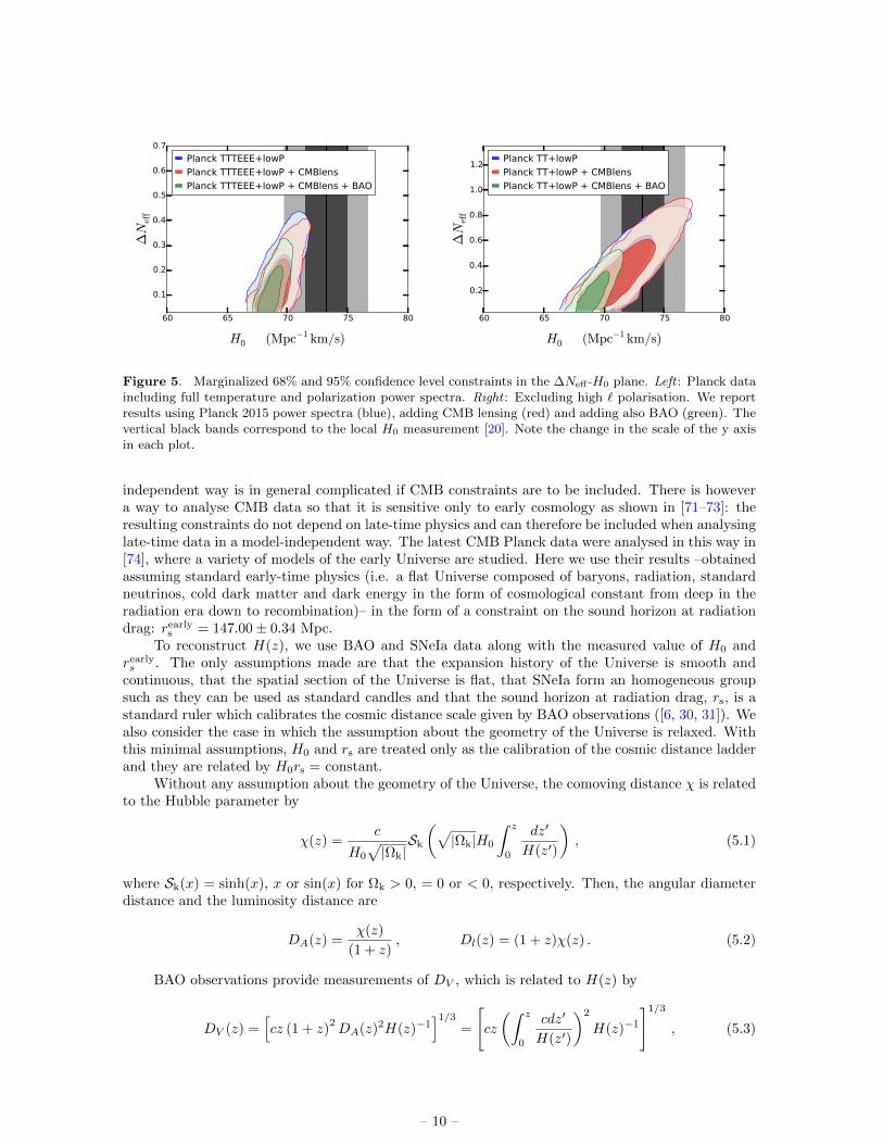
If we define ∆Neff as Neff − 3.04, it is well known that a ∆Neff > 0 would increase the CMB-inferred H0 value, bringing it closer to the locally measured one. This can be appreciated in Fig. 3,where we show the results of Planck 2015 for a model where Neff is an additional free parameter andthe extra radiation behaves like neutrinos. In the H0-Neff parameter space we show the joint 68% and95% confidence regions for Planck 2015 data (blue) and Planck 2015 + BAO data (green) obtainedfrom the Planck team’s public chains, both using polarization and temperature power spectra (left)or just temperature power spectrum and lowP (right). The vertical bands correspond to the local H0

measurement [20].A high value of Neff (∆Neff ∼ 0.4) would alleviate the tension in H0 and still be allowed by

the Planck lowP and high ` temperature power spectra and BAO data as pointed out in [20]. The“preliminary” high ` polarization data, disfavours such large ∆Neff (at ∼ 2σ level), as polarizationconstrains strongly the effective number of relativistic species.

This is however not the full story. State-of-the-art CMB data have enough statistical power tomeasure not just the effect of thisNeff on the expansion history but also on the perturbations. Neutrinodensity/pressure perturbations, bulk velocity and anisotropic stress are additional sources for thegravitational potential via the Einstein equations (see e.g., [61–63]). The effect on the perturbationsis described by the effective parameters sound speed and viscosity c2s, c

2vis [64–67]. Neutrinos have

c2s, c2vis = 1/3, 1/3, but other values describe other physics, for example a perfect relativisticfluid will have 1/3, 0 and a scalar field oscillating in a quartic potential 1, 0. Different valuesof c2s and c2vis would describe other dark radiation candidates. This parametrisation is consideredflexible enough for providing a good approximation to several alternatives to the standard case offree-streaming particles e.g., [68, 69].

Recent analyses have shown that if all Neff species have the same effective parameters c2s, c2vis,

Planck data constraints are tight [3, 70]: c2s = 0.3240 ± 0.0060, c2vis = 0.327 ± 0.037 (with fixedNeff = 3.046; Planck 2015). Moreover, the Neff constraints are not significantly affected compared tothe standard case: Neff = 3.22+0.32

−0.37 ([70]) against Neff = 3.13± 0.31 (Planck 2015) at 68% confidence

3The number of (active) neutrinos species is 3, the small correction accounts for the fact that the neutrino decouplingepoch was immediately followed by e+e− annihilation.

– 7 –

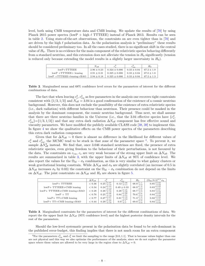
level, both using CMB temperature data and CMB lensing. We update the results of [70] by usingPlanck 2015 power spectra (lowP + high ` TTTEEE) instead of Planck 2013. Results can be seenin table 2. Using state-of-the-art observations, the constraints on are even tighter than in [70] andare driven by the high ` polarisation data. As the polarisation analysis is “preliminary” these resultsshould be considered preliminary too. In all the cases studied, there is no significant shift in the centralvalue ofH0. There is no evidence for the main component of the relativistic species behaving differentlyfrom a standard neutrino, and this extension does not alleviate the tension in H0 significantly (tensionis reduced only because extending the model results in a slightly larger uncertainty in H0).

Neff c2s c2vis H0

lowP+TTTEEE 2.96± 0.23 0.324± 0.006 0.33± 0.04 67.2± 1.9

lowP +TTTEEE+ lensing 2.91± 0.21 0.325± 0.006 0.33± 0.04 67.0± 1.8

lowP +TTTEEE+lensing+BAO 2.94± 0.18 0.325± 0.006 0.33± 0.04 67.2± 1.3

Table 2. Marginalised mean and 68% confidence level errors for the parameters of interest for the differentcombinations of data.

The fact that when leaving c2s, c2vis as free parameters in the analysis one recovers tight constraints

consistent with 1/3, 1/3 and Neff = 3.04 is a good confirmation of the existence of a cosmic neutrinobackground. However, this does not exclude the possibility of the existence of extra relativistic species(i.e., dark radiation) with different behaviour than neutrinos. Their presence could be masked in theanalysis by the dominant component, the cosmic neutrino background. Thus next, we shall assumethat there are three neutrino families in the Universe (i.e., that the 3.04 effective species have c2s,c2vis=1/3, 1/3) and that any extra dark radiation ∆Neff component has free effective sound andviscosity parameters. We have modified the publicly available CLASS code [38, 39] to implement this.In figure 4 we show the qualitative effects on the CMB power spectra of the parameters describingthis extra dark radiation component.

Given that for ∆Neff ∼ 0 there is almost no difference in the likelihood for different values ofc2s and c2vis, the MCMC tend to be stuck in that zone of the parameter space 4. To prevent it, wesample ∆N2

eff instead. We find that, once 3.046 standard neutrinos are fixed, the presence of extrarelativistic species, even giving freedom to the behaviour of their perturbations, is not favoured bythe data. The constraints on cvis, cs are very weak because of the strong upper limit on ∆Neff . Theresults are summarized in table 3, with the upper limits of ∆Neff at 95% of confidence level. Wealso report the values for the ΩM − σ8 combination, as this is very similar to what galaxy clusters orweak gravitational lensing constrain. While ∆Neff and σ8 are slightly correlated (an increase of 0.5 in∆Neff increases σ8 by 0.03) the constraint on the ΩM − σ8 combination do not depend on the limitson ∆Neff . The joint constraints on ∆Neff and H0 are shown in figure 5.

∆Neff c2s c2vis H0 (ΩM/0.3)0.5 σ8

lowP+ TTTEEE < 0.36 0.25+0.07−0.15 0.12+0.58

−0.11 68.9+1.1−0.9 0.85+0.02

−0.02

lowP+ TTTEEE+CMB lensing < 0.34 0.24+0.10−0.13 0.49± 0.33 68.9+1.2

−0.9 0.83+0.02−0.01

lowP+ TTTEEE+CMB lensing+BAO < 0.28 0.26+0.09−0.16 0.28+0.45

−0.26 68.7+0.6−0.7 0.84+0.01

−0.02

lowP + TT < 0.76 0.25+0.08−0.10 0.84+0.20

−0.51 70.6+2.6−2.0 0.84+0.03

−0.04

lowP+ TT+CMB lensing < 0.77 0.27+0.07−0.11 0.81+0.19

−0.50 71.3+1.9−2.2 0.82+0.02

−0.01

lowP+ TT+CMB lensing+BAO < 0.44 0.29+0.20−0.16 0.9+0.1

−0.7 69.0+0.9−0.8 0.84+0.01

−0.02

Table 3. Marginalised constraints for the parameters of interest for the different combinations of data. Wereport the the upper limit for ∆Neff (95% confidence level) and the highest posterior density intervals for therest of the parameters.

Should the low-level systematic present in the polarisation data be found to be sub-dominant inthe published error-budget, this finding implies that there is not much room for an extra component

4For the parameters c2vis and c2s we limit the sampling to the range [0.0, 1.1]. That is because values higher than oneare not physical and this way we also optimize the performance of the analysis, since we do not explore the parameterspace where these values are allowed to be very large in the region close to ∆Neff = 0.

– 8 –

ΛCDM ∆Neff=1,ν ∆Neff=1,φ ∆Neff=2,φ ∆Neff=0.1,c 2eff =10,c 2vis=5

0 500 1000 1500 2000 2500 30000

2000

4000

6000

DTT

`(µ

K2

)

0 500 1000 1500 2000 2500 3000

`

0.0

0.2

0.4

DTT

`/D

TT

` ΛC

DM−

1

0 500 1000 1500 2000 2500 3000200

100

0

100

200

DTE

`(µ

K2

)

0 500 1000 1500 2000 2500 3000

`

100

50

0

50

DTE

`−D

TE

` ΛC

DM(µ

K2

)

0 500 1000 1500 2000 2500 30000

10

20

30

40

50

60

DEE

`(µ

K2

)

0 500 1000 1500 2000 2500 3000

`

0.5

0.0

0.5

1.0

DEE

`/D

EE

` ΛC

DM−

1

Figure 4. CMB temperature (left), temperature and polarization cross correlation (right) and polarization(bottom) power spectra predictions for ΛCDM (red) and the following extensions: one more neutrino (blue),one scalar field (green), two scalar fields (black) and a illustrative case with extreme (non physical) values ofc2s and c2vis with ∆Neff = 0.1 (orange).

in the early universe whose density scales with the expansion like radiation but whose perturbationshave the freedom to behave like a perfect fluid, a neutrino, a scalar field or anything in between. Thisoffers a useful confirmation of one of the key standard assumptions on which the standard cosmologicalmodel is built. Also in this more general model, of the CMB data, it is the high-` polarisation whatdisfavor high values of H0. On the other hand, the freedom on the nature of the extra relativisticspecies produces a small shift in H0 towards higher values and, when high ` polarization data of theCMB are not included, our constraints are fully compatible with the direct measurement (right panelof figure 5). However, when BAO data are included, the constraint on ∆Neff is tighter, because thedegeneracy with ΩM.

5 Changing late-time cosmology

The CMB is sensitive to both late and early cosmology. When fitting the CMB power spectrumsimultaneous assumptions about the early and late cosmology must be made, with the implicationthat the physics of both epochs are entwined in the resulting constraints. Then, it is difficult todetermine what physics beyond ΛCDM would be the responsible of possible deviations from themodel. Exploring non-standard late cosmology evolution, possibly in a minimally-parametric or model

– 9 –

60 65 70 75 80

H0 (Mpc−1 km/s)

0.1

0.2

0.3

0.4

0.5

0.6

0.7∆N

eff

Planck TTTEEE+lowP

Planck TTTEEE+lowP + CMBlens

Planck TTTEEE+lowP + CMBlens + BAO

60 65 70 75 80

H0 (Mpc−1 km/s)

0.2

0.4

0.6

0.8

1.0

1.2

∆N

eff

Planck TT+lowP

Planck TT+lowP + CMBlens

Planck TT+lowP + CMBlens + BAO

Figure 5. Marginalized 68% and 95% confidence level constraints in the ∆Neff -H0 plane. Left : Planck dataincluding full temperature and polarization power spectra. Right : Excluding high ` polarisation. We reportresults using Planck 2015 power spectra (blue), adding CMB lensing (red) and adding also BAO (green). Thevertical black bands correspond to the local H0 measurement [20]. Note the change in the scale of the y axisin each plot.

independent way is in general complicated if CMB constraints are to be included. There is howevera way to analyse CMB data so that it is sensitive only to early cosmology as shown in [71–73]: theresulting constraints do not depend on late-time physics and can therefore be included when analysinglate-time data in a model-independent way. The latest CMB Planck data were analysed in this way in[74], where a variety of models of the early Universe are studied. Here we use their results –obtainedassuming standard early-time physics (i.e. a flat Universe composed of baryons, radiation, standardneutrinos, cold dark matter and dark energy in the form of cosmological constant from deep in theradiation era down to recombination)– in the form of a constraint on the sound horizon at radiationdrag: rearly

s = 147.00± 0.34 Mpc.To reconstruct H(z), we use BAO and SNeIa data along with the measured value of H0 and

rearlys . The only assumptions made are that the expansion history of the Universe is smooth and

continuous, that the spatial section of the Universe is flat, that SNeIa form an homogeneous groupsuch as they can be used as standard candles and that the sound horizon at radiation drag, rs, is astandard ruler which calibrates the cosmic distance scale given by BAO observations ([6, 30, 31]). Wealso consider the case in which the assumption about the geometry of the Universe is relaxed. Withthis minimal assumptions, H0 and rs are treated only as the calibration of the cosmic distance ladderand they are related by H0rs = constant.

Without any assumption about the geometry of the Universe, the comoving distance χ is relatedto the Hubble parameter by

χ(z) =c

H0

√|Ωk|Sk

(√|Ωk|H0

∫ z

0

dz′

H(z′)

), (5.1)

where Sk(x) = sinh(x), x or sin(x) for Ωk > 0, = 0 or < 0, respectively. Then, the angular diameterdistance and the luminosity distance are

DA(z) =χ(z)

(1 + z), Dl(z) = (1 + z)χ(z) . (5.2)

BAO observations provide measurements of DV , which is related to H(z) by

DV (z) =[cz (1 + z)

2DA(z)2H(z)−1

]1/3=

[cz

(∫ z

0

cdz′

H(z′)

)2

H(z)−1

]1/3

, (5.3)

– 10 –

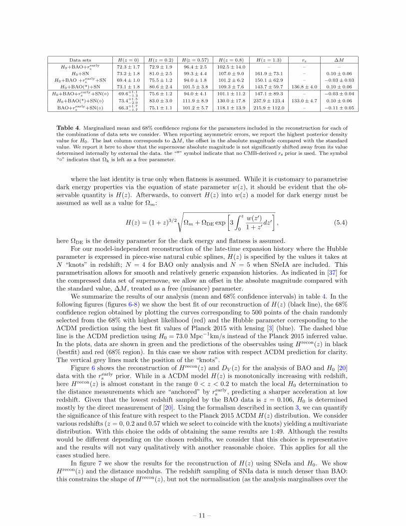
Data sets H(z = 0) H(z = 0.2) H(z = 0.57) H(z = 0.8) H(z = 1.3) rs ∆M

H0+BAO+rearlys 72.3± 1.7 72.9± 1.9 96.4± 2.5 102.5± 14.0 – – –

H0+SN 73.2± 1.8 81.0± 2.5 99.3± 4.4 107.0± 9.0 161.9± 73.1 – 0.10± 0.06

H0+BAO +rearlys +SN 69.4± 1.0 75.5± 1.2 94.0± 1.8 101.2± 6.2 150.1± 62.9 – −0.03± 0.03

H0+BAO(*)+SN 73.1± 1.8 80.6± 2.4 101.5± 3.8 109.3± 7.6 143.7± 59.7 136.8± 4.0 0.10± 0.06

H0+BAO+rearlys +SN() 69.6+1.1−1.3 75.6± 1.2 94.0± 4.1 101.1± 11.2 147.1± 89.3 – −0.03± 0.04

H0+BAO(*)+SN() 73.4+1.5−2.0 83.0± 3.0 111.9± 8.9 130.0± 17.8 237.9± 123.4 133.0± 4.7 0.10± 0.06

BAO+rearlys +SN() 66.3+1.7−1.7 75.1± 1.1 101.2± 5.7 118.1± 13.9 215.9± 112.0 – −0.11± 0.05

Table 4. Marginalized mean and 68% confidence regions for the parameters included in the reconstruction for each ofthe combinations of data sets we consider. When reporting asymmetric errors, we report the highest posterior densityvalue for H0. The last column corresponds to ∆M , the offset in the absolute magnitude compared with the standardvalue. We report it here to show that the supernovae absolute magnitude is not significantly shifted away from its valuedetermined internally by external the data. the “*” symbol indicate that no CMB-derived rs prior is used. The symbol“” indicates that Ωk is left as a free parameter.

where the last identity is true only when flatness is assumed. While it is customary to parametrisedark energy properties via the equation of state parameter w(z), it should be evident that the ob-servable quantity is H(z). Afterwards, to convert H(z) into w(z) a model for dark energy must beassumed as well as a value for Ωm:

H(z) = (1 + z)3/2

√Ωm + ΩDE exp

[3

∫ z

0

w(z′)

1 + z′dz′], (5.4)

here ΩDE is the density parameter for the dark energy and flatness is assumed.For our model-independent reconstruction of the late-time expansion history where the Hubble

parameter is expressed in piece-wise natural cubic splines, H(z) is specified by the values it takes atN “knots” in redshift; N = 4 for BAO only analysis and N = 5 when SNeIA are included. Thisparametrisation allows for smooth and relatively generic expansion histories. As indicated in [37] forthe compressed data set of supernovae, we allow an offset in the absolute magnitude compared withthe standard value, ∆M , treated as a free (nuisance) parameter.

We summarize the results of our analysis (mean and 68% confidence intervals) in table 4. In thefollowing figures (figures 6-8) we show the best fit of our reconstruction of H(z) (black line), the 68%confidence region obtained by plotting the curves corresponding to 500 points of the chain randomlyselected from the 68% with highest likelihood (red) and the Hubble parameter corresponding to theΛCDM prediction using the best fit values of Planck 2015 with lensing [3] (blue). The dashed blueline is the ΛCDM prediction using H0 = 73.0 Mpc−1km/s instead of the Planck 2015 inferred value.In the plots, data are shown in green and the predictions of the observables using Hrecon(z) in black(bestfit) and red (68% region). In this case we show ratios with respect ΛCDM prediction for clarity.The vertical grey lines mark the position of the “knots”.

Figure 6 shows the reconstruction of Hrecon(z) and DV (z) for the analysis of BAO and H0 [20]data with the rearly

s prior. While in a ΛCDM model H(z) is monotonically increasing with redshift,here Hrecon(z) is almost constant in the range 0 < z < 0.2 to match the local H0 determination tothe distance measurements which are “anchored” by rearly

s , predicting a sharper acceleration at lowredshift. Given that the lowest redshift sampled by the BAO data is z = 0.106, H0 is determinedmostly by the direct measurement of [20]. Using the formalism described in section 3, we can quantifythe significance of this feature with respect to the Planck 2015 ΛCDM H(z) distribution. We considervarious redshifts (z = 0, 0.2 and 0.57 which we select to coincide with the knots) yielding a multivariatedistribution. With this choice the odds of obtaining the same results are 1:49. Although the resultswould be different depending on the chosen redshifts, we consider that this choice is representativeand the results will not vary qualitatively with another reasonable choice. This applies for all thecases studied here.

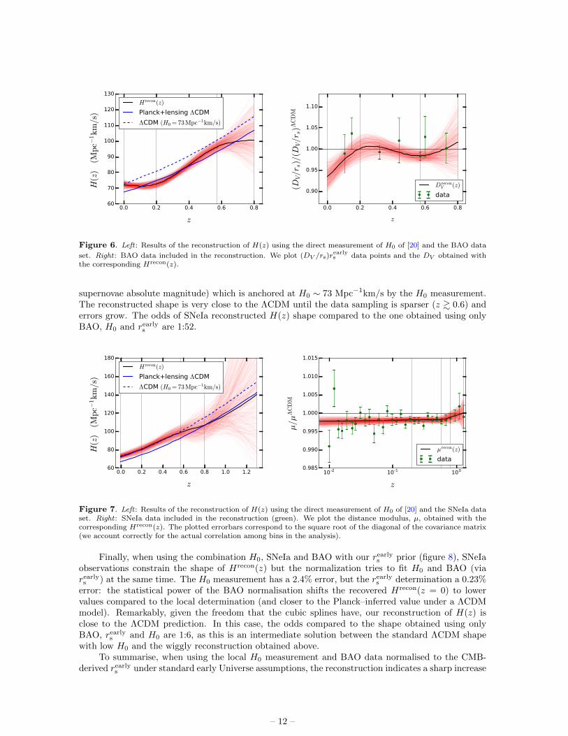
In figure 7 we show the results for the reconstruction of H(z) using SNeIa and H0. We showHrecon(z) and the distance modulus. The redshift sampling of SNIa data is much denser than BAO:this constrains the shape of Hrecon(z), but not the normalisation (as the analysis marginalises over the

– 11 –

0.0 0.2 0.4 0.6 0.8

z

60

70

80

90

100

110

120

130H

(z)

(Mpc−

1km/s

) H recon(z)

Planck+lensing ΛCDM

ΛCDM (H0 = 73Mpc−1km/s)

0.0 0.2 0.4 0.6 0.8

z

0.90

0.95

1.00

1.05

1.10

(DV/r

s)/

(DV/r

s)Λ

CD

M

D reconV (z)

data

Figure 6. Left : Results of the reconstruction of H(z) using the direct measurement of H0 of [20] and the BAO data

set. Right : BAO data included in the reconstruction. We plot (DV /rs)rearlys data points and the DV obtained with

the corresponding Hrecon(z).

supernovae absolute magnitude) which is anchored at H0 ∼ 73 Mpc−1km/s by the H0 measurement.The reconstructed shape is very close to the ΛCDM until the data sampling is sparser (z & 0.6) anderrors grow. The odds of SNeIa reconstructed H(z) shape compared to the one obtained using onlyBAO, H0 and rearly

s are 1:52.

0.0 0.2 0.4 0.6 0.8 1.0 1.2

z

60

80

100

120

140

160

180

H(z

)(M

pc−

1km/s

)

H recon(z)

Planck+lensing ΛCDM

ΛCDM (H0 = 73Mpc−1km/s)

10-2 10-1 100

z

0.985

0.990

0.995

1.000

1.005

1.010

1.015

µ/µ

ΛC

DM

µrecon(z)

data

Figure 7. Left : Results of the reconstruction of H(z) using the direct measurement of H0 of [20] and the SNeIa dataset. Right : SNeIa data included in the reconstruction (green). We plot the distance modulus, µ, obtained with thecorresponding Hrecon(z). The plotted errorbars correspond to the square root of the diagonal of the covariance matrix(we account correctly for the actual correlation among bins in the analysis).

Finally, when using the combination H0, SNeIa and BAO with our rearlys prior (figure 8), SNeIa

observations constrain the shape of Hrecon(z) but the normalization tries to fit H0 and BAO (viarearlys ) at the same time. The H0 measurement has a 2.4% error, but the rearly

s determination a 0.23%error: the statistical power of the BAO normalisation shifts the recovered Hrecon(z = 0) to lowervalues compared to the local determination (and closer to the Planck–inferred value under a ΛCDMmodel). Remarkably, given the freedom that the cubic splines have, our reconstruction of H(z) isclose to the ΛCDM prediction. In this case, the odds compared to the shape obtained using onlyBAO, rearly

s and H0 are 1:6, as this is an intermediate solution between the standard ΛCDM shapewith low H0 and the wiggly reconstruction obtained above.

To summarise, when using the local H0 measurement and BAO data normalised to the CMB-derived rearly

s under standard early Universe assumptions, the reconstruction indicates a sharp increase

– 12 –

0.0 0.2 0.4 0.6 0.8 1.0 1.2

z

60

80

100

120

140

160

180H

(z)

(Mpc−

1km/s)

H recon(z)

Planck+lensing ΛCDM

ΛCDM (H0 = 73Mpc−1km/s)

0.0 0.2 0.4 0.6 0.8

z

0.90

0.95

1.00

1.05

1.10

(DV/r s

)/(D

V/r s

)ΛC

DM

D reconV (z)

data

10-2 10-1 100

z

0.985

0.990

0.995

1.000

1.005

1.010

1.015

µ/µ

ΛC

DM

µrecon(z)

data

Figure 8. Left : Results of the reconstruction of H(z) using the direct measurement of H0 of [20], BAO and SNeIadata set with a CMB-derived rs prior. Middle and right : Observational data included in the reconstruction (green), asin the previous cases, and the prediction using the corresponding Hrecon(z).

in the cosmic acceleration rate (H(z) ∼constant) at z < 0.2, where the BAO data have little statisticalpower. A dark energy equation of state parameter w < −1 (or dropping recently below −1) wouldfit the bill. However, when including SNeIa the shape of the expansion history is constrained not todeviate significantly from that of ΛCDM (at z < 0.6 where there are many data points) and thusonly the normalisation can adjust, taking a value intermediate between the low and high redshift“anchors”, as H0rs ≈ constant. Thus a phantom dark energy is not favoured by the data. Below wewill show that relaxing the flatness assumption does not change the results qualitatively.

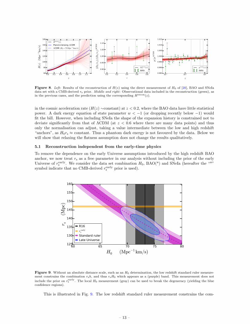
5.1 Reconstruction independent from the early-time physics

To remove the dependence on the early Universe assumptions introduced by the high redshift BAOanchor, we now treat rs as a free parameter in our analysis without including the prior of the earlyUniverse of rearly

s . We consider the data set combination H0, BAO(*) and SNeIa (hereafter the “*”symbol indicate that no CMB-derived rearly

s prior is used).

60 65 70 75 80

H0 (Mpc−1 km/s)

125

130

135

140

145

150

155

160

r s(M

pc)

R16

r earlys

Standard ruler

Late Universe

Figure 9. Without an absolute distance scale, such as an H0 determination, the low redshift standard ruler measure-ment constrains the combination rsh, and thus rsH0 which appears as a (purple) band. This measurement does not

include the prior on rearlys . The local H0 measurement (gray) can be used to break the degeneracy (yielding the blue

confidence regions).

This is illustrated in Fig. 9. The low redshift standard ruler measurement constrains the com-

– 13 –

bination rsh which is reported here as a band in the H0-rs plane, constraining H0rs = constant.This constraint only relies on the BAO yielding a standard ruler (of unknown length), on SNe beingstandard candles (of unknown luminosity), on spatial flatness and on a smooth expansion history.The local H0 measurement or the early-time rs “anchors” can be used to break the degeneracy. Thers measurement relies on early-time physics assumptions (i.e. the value of Neff , Y BBN

P , recombinationphysics, epoch of matter-radiation equality etc.). The H0 measurement relies on local calibrators ofthe cosmic distance ladder.

0.0 0.2 0.4 0.6 0.8 1.0 1.2

z

60

80

100

120

140

160

180

H(z

)(M

pc−

1km/s)

H recon(z)

Planck+lensing ΛCDM

ΛCDM (H0 = 73Mpc−1km/s)

0.0 0.2 0.4 0.6 0.8

z

0.90

0.95

1.00

1.05

1.10

(DV/r s

)/(D

V/r s

)ΛC

DM

D reconV (z)

data

10-2 10-1 100

z

0.985

0.990

0.995

1.000

1.005

1.010

1.015

µ/µ

ΛC

DM

µrecon(z)

data

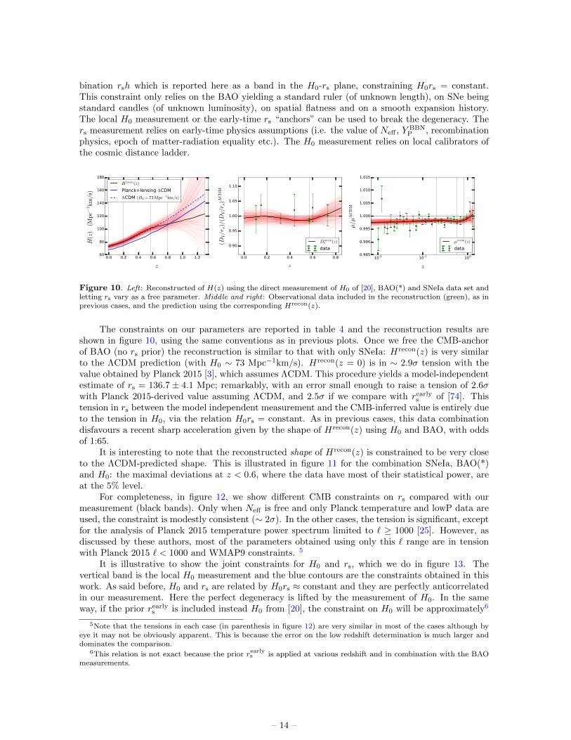
Figure 10. Left : Reconstructed of H(z) using the direct measurement of H0 of [20], BAO(*) and SNeIa data set andletting rs vary as a free parameter. Middle and right : Observational data included in the reconstruction (green), as inprevious cases, and the prediction using the corresponding Hrecon(z).

The constraints on our parameters are reported in table 4 and the reconstruction results areshown in figure 10, using the same conventions as in previous plots. Once we free the CMB-anchorof BAO (no rs prior) the reconstruction is similar to that with only SNeIa: Hrecon(z) is very similarto the ΛCDM prediction (with H0 ∼ 73 Mpc−1km/s). Hrecon(z = 0) is in ∼ 2.9σ tension with thevalue obtained by Planck 2015 [3], which assumes ΛCDM. This procedure yields a model-independentestimate of rs = 136.7 ± 4.1 Mpc; remarkably, with an error small enough to raise a tension of 2.6σwith Planck 2015-derived value assuming ΛCDM, and 2.5σ if we compare with rearly

s of [74]. Thistension in rs between the model independent measurement and the CMB-inferred value is entirely dueto the tension in H0, via the relation H0rs = constant. As in previous cases, this data combinationdisfavours a recent sharp acceleration given by the shape of Hrecon(z) using H0 and BAO, with oddsof 1:65.

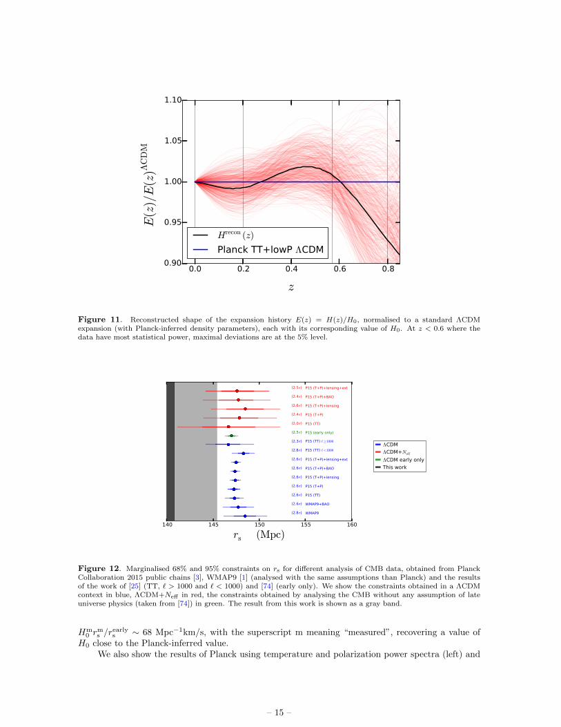
It is interesting to note that the reconstructed shape of Hrecon(z) is constrained to be very closeto the ΛCDM-predicted shape. This is illustrated in figure 11 for the combination SNeIa, BAO(*)and H0: the maximal deviations at z < 0.6, where the data have most of their statistical power, areat the 5% level.

For completeness, in figure 12, we show different CMB constraints on rs compared with ourmeasurement (black bands). Only when Neff is free and only Planck temperature and lowP data areused, the constraint is modestly consistent (∼ 2σ). In the other cases, the tension is significant, exceptfor the analysis of Planck 2015 temperature power spectrum limited to ` ≥ 1000 [25]. However, asdiscussed by these authors, most of the parameters obtained using only this ` range are in tensionwith Planck 2015 ` < 1000 and WMAP9 constraints. 5

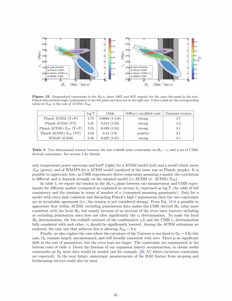
It is illustrative to show the joint constraints for H0 and rs, which we do in figure 13. Thevertical band is the local H0 measurement and the blue contours are the constraints obtained in thiswork. As said before, H0 and rs are related by H0rs ≈ constant and they are perfectly anticorrelatedin our measurement. Here the perfect degeneracy is lifted by the measurement of H0. In the sameway, if the prior rearly

s is included instead H0 from [20], the constraint on H0 will be approximately6

5Note that the tensions in each case (in parenthesis in figure 12) are very similar in most of the cases although byeye it may not be obviously apparent. This is because the error on the low redshift determination is much larger anddominates the comparison.

6This relation is not exact because the prior rearlys is applied at various redshift and in combination with the BAO

measurements.

– 14 –

0.0 0.2 0.4 0.6 0.8

z

0.90

0.95

1.00

1.05

1.10

E(z

)/E

(z)Λ

CD

M

Hrecon (z)

Planck TT+lowP ΛCDM

Figure 11. Reconstructed shape of the expansion history E(z) = H(z)/H0, normalised to a standard ΛCDMexpansion (with Planck-inferred density parameters), each with its corresponding value of H0. At z < 0.6 where thedata have most statistical power, maximal deviations are at the 5% level.

140 145 150 155 160

rs (Mpc)

0

5

10

15

20

25

30

WMAP9

WMAP9+BAO

P15 (TT)

P15 (T+P)

P15 (T+P)+lensing

P15 (T+P)+BAO

P15 (T+P)+lensing+ext

P15 (TT) `<1000

P15 (TT) `≥1000

P15 (early only)

P15 (TT)

P15 (T+P)

P15 (T+P)+lensing

P15 (T+P)+BAO

P15 (T+P)+lensing+ext

(2.8σ)

(2.6σ)

(2.6σ)

(2.6σ)

(2.6σ)

(2.6σ)

(2.6σ)

(2.8σ)

(2.3σ)

(2.5σ)

(2.0σ)

(2.4σ)

(2.6σ)

(2.4σ)

(2.5σ)

ΛCDMΛCDM+Neff

ΛCDM early onlyThis work

Figure 12. Marginalised 68% and 95% constraints on rs for different analysis of CMB data, obtained from PlanckCollaboration 2015 public chains [3], WMAP9 [1] (analysed with the same assumptions than Planck) and the resultsof the work of [25] (TT, ` > 1000 and ` < 1000) and [74] (early only). We show the constraints obtained in a ΛCDMcontext in blue, ΛCDM+Neff in red, the constraints obtained by analysing the CMB without any assumption of lateuniverse physics (taken from [74]) in green. The result from this work is shown as a gray band.

Hm0 r

ms /r

earlys ∼ 68 Mpc−1km/s, with the superscript m meaning “measured”, recovering a value of

H0 close to the Planck-inferred value.We also show the results of Planck using temperature and polarization power spectra (left) and

– 15 –

60 65 70 75 80

H0 (Mpc−1 km/s)

125

130

135

140

145

150

155

160r s

(Mpc)

Late UniversePlanck ΛCDM

Planck ΛCDM+Neff

WMAP ΛCDM2.55

2.70

2.85

3.00

3.15

3.30

3.45

Neff

60 65 70 75 80

H0 (Mpc−1 km/s)

125

130

135

140

145

150

155

160

r s(M

pc)

Late UniversePlanck ΛCDM

Planck ΛCDM+Neff

WMAP ΛCDM2.4

2.6

2.8

3.0

3.2

3.4

3.6

3.8

4.0

Neff

Figure 13. Marginalized constraints in the H0-rs plane (68% and 95% regions) for the cases discussed in the text.Planck data includes high ` polarization in the left panel and does not in the right one. Color-coded are the correspondingvalues of Neff in the case of ΛCDM+Neff .

log T Odds Jeffrey’s modified scale Gaussian tension

Planck ΛCDM (T+P) 4.75 0.0086 (1:116) strong 3.7

Planck ΛCDM (TT) 4.31 0.013 (1:76) strong 3.5

Planck ΛCDM+Neff (T+P) 3.55 0.029 (1:34) strong 3.1

Planck ΛCDM+Neff (TT) 2.02 0.13 (1:8) positive 2.1

WMAP ΛCDM 3.59 0.027 (1:37) strong 3.1

Table 5. Two dimensional tension between the low redshift joint constraints on H0 − rs and a set of CMB-derived constraints. See section 3 for details.

only temperature power spectrum and lowP (right) for a ΛCDM model (red) and a model which variesNeff (green); and of WMAP9 for a ΛCDM model (analysed in the same way as Planck, purple). It ispossible to appreciate how, as CMB experiments derive constraints assuming a model, the correlationis different and it depends strongly on the adopted model (i.e ΛCDM vs. ΛCDM+Neff).

In table 5, we report the tension in the H0-rs plane between our measurement and CMB exper-iments for different models (computed as explained in section 3), expressed as log T , the odds of fullconsistency and the tensions in terms of number of σ (computed assuming gaussianity). Only for amodel with extra dark radiation and discarding Planck’s high ` polarisation data the two constraintsare in acceptable agreement (i.e., the tension is not considered strong). From Fig. 13 it is possible toappreciate that within ΛCDM, excluding polarisation data makes the CMB–derived H0 value moreconsistent with the local H0, but mainly because of an increase of the error bars; however includingor excluding polarisation data does not alter significantly the rs determination. To make the localH0 determination, the low-redshift estimate of the combination rsh and the CMB rs determinationfully consistent with each other, rs should be significantly lowered. Among the ΛCDM extensions weexplored, the only one that achieves this is allowing Neff ∼ 3.4.

Finally, we also explore the case where the curvature of the Universe is not fixed to Ωk = 0.In thiscase, Ωk remains largely unconstrained, and still broadly consistent with zero. There is no significantshift in the rest of parameters, but the error bars are larger. The constraints are summarized in thebottom rows of table 4. Given the freedom of our expansion history reconstruction, to obtain usefulconstraints on Ωk more data would be needed (see for example, [30, 31] where curvature constraintsare reported). In the near future, anisotropic measurements of the BAO feature from on-going andforthcoming surveys could also be used.

– 16 –

6 Discussion and Conclusions

The standard ΛCDM model with only a handful of parameters, provides an excellent description of ahost of cosmological observations with remarkably few exceptions. The most notable and persistentone is the local determination of the Hubble constant H0, which, with the recent improvement by[20], presents a ∼ 3σ tension with respect to the value inferred by the Planck Collaboration (as-suming ΛCDM). The CMB is mostly sensitive to early-Universe physics, and the CMB-inferred H0

measurement thus depends on assumptions about both early time and late-time physics. A relatedquantity that the CMB can measure in a way that does not depend on late-time physics is the soundhorizon at radiation drag, rs. This measurement however is still model-dependent in that it relieson standard assumptions about early-time physics. On the other hand the local measurement of H0

is model-independent as it does not depend on cosmological assumptions. As this work was near-ing completion, new quasar time-delay cosmography data became available [24]. Within the ΛCDMmodel these provide an H0 constraint centered around 72 Mpc−1km/s, with a 4% error and thusshows reduced tension.

The two parameters rs and H0 are strictly related when we consider also BAO observations.Expansion history probes such as BAO and SNIa can provide a model-independent estimate of the low-redshift standard ruler, constraining directly the combination rsh (with H0 = h× 100 Mpc−1km/s).Thus rs and H0 provide absolute scales for distance measurements (anchors) at opposite ends ofthe observable Universe. In the absence of systematic errors in the measurements, if the standardcosmological model is the correct model, indirect (model-dependent) and direct (model-independent)constraints on these parameters should agree. The tension could thus provide evidence of physicsbeyond the standard model (or unaccounted systematic errors).

We have performed a complete cosmological study of the current tension between the inferredvalue of H0 from the latest CMB data (as provided by the Planck satellite) [3] and its direct mea-surement, with the recent update from [20]. This reflects into a tension between cosmological model-dependent and model-independent constraints on rs.

We first have explored models for deviations from the standard ΛCDM in the early-Universephysics. When including CMB data alone (or in combination with geometric measurements thatdo not rely on the H0 anchor such as BAO) we find no evidence for deviations from the standardΛCDM model and in particular no evidence for extra effective relativistic species beyond three activeneutrinos. This conclusion is unchanged if we allow additional freedom in the behaviour of theperturbations, both in all relativistic species or only in the additional ones.

Therefore we put limits on the possible presence of a Universe component whose mean energyscales like radiation with the Universe expansion but which perturbations could behave like radiation,a perfect fluid, a scalar field or anything else in between. On the other hand the value for the Hubbleconstant inferred by these analyses and other promising modifications of early-time physics, is alwayssignificantly lower than the local measurement of [20]. Should the low-level systematics present in thehigh ` “preliminary” Planck polarisation data be found to be non-negligible, the TEEE data shouldnot be included in the analysis. In this case, including only the “recommended” baseline of low `temperature and polarisation data and only temperature for high `, the tight limits relax and thetension disappears for a cosmological model with extra dark radiation corresponding to ∆Neff ∼ 0.4.However the tension appears (but at an acceptable level) again when BAO data is included. Theconstraints on the effective parameters which describe the behaviour of the extra radiation in termsof perturbations are too weak to discriminate among the different candidates.

Another possible way to reconcile the CMB-derived H0 value and the local measurement is toallow deviations from the standard late-time expansion history of the Universe. Rather than invokingspecific models we have reconstructed the expansion history in a model-independent, minimally para-metric way. Our method to reconstruct H(z) does not rely on any model and only require minimalassumptions. These are: SNeIa form a homogeneous group and can be used as standard candles,rs is a standard ruler for BAO corresponding to the sound horizon at radiation drag, the expansionhistory is smooth and continuous and the Universe is spatially flat. When only using BAO, and theH0 measurement with an early Universe rs prior, the reconstructed H(z) shows a sharp increase in

– 17 –

acceleration at low redshift, such as that provided by a phantom equation of state parameter for darkenergy. However when SNeIa are included, the shape of H(z) cannot deviate significantly from thatof a ΛCDM, disfavouring therefore the phantom dark energy solution. When the CMB rs prior isremoved, this procedure yields a model-independent determination of rs (and the expansion history)without any assumption on the early Universe. The rs value so obtained is significantly lower thanthat obtained from the CMB assuming standard early-time physics (2.6σ tension). When we relaxthe assumption about the flatness of the Universe, the curvature remains largely unconstrained andthe error on the other parameters grow slightly. We do not find significant shifts in the rest of theparameters.

Of course this hinges on identifying the BAO standard ruler with the sound horizon at radiationdrag. Several processes have been proposed that could displace the BAO feature, the most importantbeing non-linearities, bias e.g., [75, 76] and non-zero baryon-dark matter relative velocity [77–79].These effects however have been found to be below current errors [80–82] and below the 1% level. Itis therefore hard to imagine how these effects could introduce the 5− 7% shift required to solve thetension.

In summary, because the shape of the expansion history is tightly constrained by current data,in a model–independent way, the H0 tension can be restated as a mis-match in the normalisationof the cosmic distance ladder between the two anchors: H0 at low redshift and rs at high redshift.In the absence of systematic errors, especially in the high ` CMB polarisation data and/or in thelocal H0 measurement, the mismatch suggest reconsidering the standard assumptions about early-time physics. Should the “preliminary” high ` CMB polarisation data be found to be affected bysignificant systematics and excluded from the analysis, the mismatch could be resolved by allowingan extra component behaving like dark radiation at the background level with a ∆Neff ∼ 0.4. Othernew physics in the early Universe that reduce the CMB-inferred sound horizon at radiation drag by∼ 10 Mpc (6%) would have the same effect.

Acknowledgments

We thank Graeme Addison, Alan Heavens and Antonio J. Cuesta for valuable discussion during thedevelopment of this study, which helped to improve this work. JLB is supported by the SpanishMINECO under grant BES-2015-071307, co-funded by the ESF. Funding for this work was partiallyprovided by the Spanish MINECO under projects AYA2014-58747-P and MDM-2014- 0369 of ICCUB(Unidad de Excelencia Maria de Maeztu). JLB acknowledges hospitality of Radcliffe Institute forAdvanced Study, Harvard University.

Based on observations obtained with Planck (http://www.esa.int/Planck), an ESA science mis-sion with instruments and contributions directly funded by ESA Member States, NASA, and Canada.

Funding for SDSS-III has been provided by the Alfred P. Sloan Foundation, the ParticipatingInstitutions, the National Science Foundation, and the U.S. Department of Energy Office of Science.The SDSS-III web site is http://www.sdss3.org/.

SDSS-III is managed by the Astrophysical Research Consortium for the Participating Institutionsof the SDSS-III Collaboration including the University of Arizona, the Brazilian Participation Group,Brookhaven National Laboratory, Carnegie Mellon University, University of Florida, the French Par-ticipation Group, the German Participation Group, Harvard University, the Instituto de Astrofisicade Canarias, the Michigan State/Notre Dame/JINA Participation Group, Johns Hopkins University,Lawrence Berkeley National Laboratory, Max Planck Institute for Astrophysics, Max Planck Insti-tute for Extraterrestrial Physics, New Mexico State University, New York University, Ohio StateUniversity, Pennsylvania State University, University of Portsmouth, Princeton University, the Span-ish Participation Group, University of Tokyo, University of Utah, Vanderbilt University, Universityof Virginia, University of Washington, and Yale University.

References

[1] G. Hinshaw, D. Larson, E. Komatsu, D. N. Spergel, C. L. Bennett, J. Dunkley, M. R. Nolta,M. Halpern, R. S. Hill, N. Odegard, L. Page, K. M. Smith, J. L. Weiland, B. Gold, N. Jarosik,

– 18 –

A. Kogut, M. Limon, S. S. Meyer, G. S. Tucker, E. Wollack, and E. L. Wright, “Nine-year WilkinsonMicrowave Anisotropy Probe (WMAP) Observations: Cosmological Parameter Results,”Astrophys.J.Sup 208 (Oct., 2013) 19, arXiv:1212.5226.

[2] C. L. Bennett, D. Larson, J. L. Weiland, N. Jarosik, G. Hinshaw, N. Odegard, K. M. Smith, R. S. Hill,B. Gold, M. Halpern, E. Komatsu, M. R. Nolta, L. Page, D. N. Spergel, E. Wollack, J. Dunkley,A. Kogut, M. Limon, S. S. Meyer, G. S. Tucker, and E. L. Wright, “Nine-year Wilkinson MicrowaveAnisotropy Probe (WMAP) Observations: Final Maps and Results,” Astrophys.J.Sup. 208 (Oct., 2013)20, arXiv:1212.5225.

[3] Planck Collaboration, P. A. R. Ade et al., “Planck 2015 results. XIII. Cosmological parameters,”arXiv:1502.01589 [astro-ph.CO].

[4] e. a. Anderson L., “The clustering of galaxies in the SDSS-III Baryon Oscillation Spectroscopic Survey:baryon acoustic oscillations in the Data Releases 10 and 11 Galaxy samples,” Mon. Not. Roy. Astron.Soc. 441 (June, 2014) 24–62, arXiv:1312.4877.

[5] A. J. Cuesta, M. Vargas-Magana, F. Beutler, A. S. Bolton, J. R. Brownstein, D. J. Eisenstein,H. Gil-Marın, S. Ho, C. K. McBride, C. Maraston, N. Padmanabhan, W. J. Percival, B. A. Reid, A. J.Ross, N. P. Ross, A. G. Sanchez, D. J. Schlegel, D. P. Schneider, D. Thomas, J. Tinker, R. Tojeiro,L. Verde, and M. White, “The clustering of galaxies in the SDSS-III Baryon Oscillation SpectroscopicSurvey: baryon acoustic oscillations in the correlation function of LOWZ and CMASS galaxies in DataRelease 12,” Mon. Not. Roy. Astron. Soc. 457 (Apr., 2016) 1770–1785, arXiv:1509.06371.

[6] A. J. Cuesta, L. Verde, A. Riess, and R. Jimenez, “Calibrating the cosmic distance scale ladder: therole of the sound horizon scale and the local expansion rate as distance anchors,” Mon. Not. Roy.Astron. Soc. 448 no. 4, (2015) 3463–3471, arXiv:1411.1094 [astro-ph.CO].

[7] E. e. a. Aubourg, “Cosmological implications of baryon acoustic oscillation measurements,” Phys. Rev.D 92 no. 12, (Dec., 2015) 123516, arXiv:1411.1074.

[8] A. G. Riess, L. Macri, S. Casertano, H. Lampeitl, H. C. Ferguson, A. V. Filippenko, S. W. Jha, W. Li,and R. Chornock, “A 3% Solution: Determination of the Hubble Constant with the Hubble SpaceTelescope and Wide Field Camera 3,” Astrophys. J. 730 (2011) 119, arXiv:1103.2976 [astro-ph.CO].[Erratum: Astrophys. J.732,129(2011)].

[9] V. Marra, L. Amendola, I. Sawicki, and W. Valkenburg, “Cosmic Variance and the Measurement of theLocal Hubble Parameter,” Physical Review Letters 110 no. 24, (June, 2013) 241305, arXiv:1303.3121[astro-ph.CO].

[10] L. Verde, P. Protopapas, and R. Jimenez, “Planck and the local Universe: Quantifying the tension,”Physics of the Dark Universe 2 (Sept., 2013) 166–175, arXiv:1306.6766 [astro-ph.CO].

[11] C. L. Bennett, D. Larson, J. L. Weiland, and G. Hinshaw, “The 1% Concordance Hubble Constant,”Astrophys. J. 794 (Oct., 2014) 135, arXiv:1406.1718.

[12] Planck Collaboration, P. A. R. Ade, N. Aghanim, C. Armitage-Caplan, M. Arnaud, M. Ashdown,F. Atrio-Barandela, J. Aumont, C. Baccigalupi, A. J. Banday, and et al., “Planck 2013 results. XVI.Cosmological parameters,” Astron. Astrophys. 571 (Nov., 2014) A16, arXiv:1303.5076.

[13] G. Efstathiou, “H0 revisited,” Mon. Not. Roy. Astron. Soc. 440 (May, 2014) 1138–1152,arXiv:1311.3461.

[14] E. M. L. Humphreys, M. J. Reid, J. M. Moran, L. J. Greenhill, and A. L. Argon, “Toward a NewGeometric Distance to the Active Galaxy NGC 4258. III. Final Results and the Hubble Constant,”Astrophys. J. 775 (Sept., 2013) 13, arXiv:1307.6031.

[15] M. Wyman, D. H. Rudd, R. A. Vanderveld, and W. Hu, “Neutrinos Help Reconcile PlanckMeasurements with the Local Universe,” Physical Review Letters 112 no. 5, (Feb., 2014) 051302,arXiv:1307.7715 [astro-ph.CO].

[16] C. Dvorkin, M. Wyman, D. H. Rudd, and W. Hu, “Neutrinos help reconcile Planck measurements withboth the early and local Universe,” Phys. Rev. D 90 no. 8, (Oct., 2014) 083503, arXiv:1403.8049.

[17] B. Leistedt, H. V. Peiris, and L. Verde, “No New Cosmological Concordance with Massive SterileNeutrinos,” Physical Review Letters 113 no. 4, (July, 2014) 041301, arXiv:1404.5950.

– 19 –

[18] Planck Collaboration, P. A. R. Ade, N. Aghanim, M. Arnaud, M. Ashdown, J. Aumont,C. Baccigalupi, A. J. Banday, R. B. Barreiro, N. Bartolo, and et al., “Planck 2015 results. XIV. Darkenergy and modified gravity,” ArXiv e-prints (Feb., 2015) , arXiv:1502.01590.

[19] E. Di Valentino, A. Melchiorri and J. Silk, “Reconciling Planck with the local value of H0 in extendedparameter space,” ArXiv e-prints (Jun., 2016) , arXiv:1606.00634.

[20] A. G. Riess, L. M. Macri, S. L. Hoffmann, D. Scolnic, S. Casertano, A. V. Filippenko, B. E. Tucker,M. J. Reid, D. O. Jones, J. M. Silverman, R. Chornock, P. Challis, W. Yuan, and R. J. Foley, “A 2.4%Determination of the Local Value of the Hubble Constant,” Astrophys. J. 826 (July, 2016) 56, ,arXiv:1604.01424.

[21] Planck Collaboration, N. Aghanim, et al., “Planck intermediate results. XLVI. Reduction of large-scalesystematic effects in HFI polarization maps and estimation of the reionization optical depth,” ArXive-prints (May, 2016) , arXiv:1605.02985.

[22] S. Casertano, A. G. Riess, B. Bucciarelli, and M. G. Lattanzi, “A test of Gaia Data Release 1parallaxes: implications for the local distance scale,” ArXiv e-prints (Sept., 2016) , arXiv:1609.05175.

[23] S. H. Suyu and et al.., “H0LiCOW I. H0 Lenses in COSMOGRAIL’s Wellspring: Program Overview,”ArXiv e-prints (June, 2016) , arXiv:1607.00017.

[24] V. Bonvin and et al., “H0LiCOW V. New COSMOGRAIL time delays of HE0435-1223: H0 to 3.8%precision from strong lensing in a flat ΛCDM model,” arXiv:1607.01790v1.

[25] G. E. Addison, Y. Huang, D. J. Watts, C. L. Bennett, M. Halpern, G. Hinshaw, and J. L. Weiland,“Quantifying Discordance in the 2015 Planck CMB Spectrum,” Astrophys. J. 818 (Feb., 2016) 132,arXiv:1511.00055.

[26] Planck Collaboration, N. Aghanim, et al., “Planck 2016 intermediate results. LI. Features in the cosmicmicrowave background temperature power spectrum and shifts in cosmological parameters,” ArXive-prints (Aug., 2016) , arXiv:1608.02487.

[27] D. J. Eisenstein and W. Hu, “Baryonic Features in the Matter Transfer Function,” Astrophys. J. 496(Mar., 1998) 605–614, astro-ph/9709112.

[28] J. Hamann, S. Hannestad, J. Lesgourgues, C. Rampf, and Y. Y. Y. Wong, “Cosmological parametersfrom large scale structure - geometric versus shape information,” JCAP 7 (July, 2010) 022,arXiv:1003.3999.

[29] R. Jimenez and A. Loeb, “Constraining Cosmological Parameters Based on Relative Galaxy Ages,”Astrophys. J. 573 (July, 2002) 37–42, astro-ph/0106145.

[30] A. Heavens, R. Jimenez, and L. Verde, “Standard rulers, candles, and clocks from the low-redshiftUniverse,” Phys. Rev. Lett. 113 no. 24, (2014) 241302, arXiv:1409.6217 [astro-ph.CO].

[31] L. Verde, J. L. Bernal, A. Heavens, and R. Jimenez, “The length of the local standard ruler,” ArXive-prints (July, 2016) , arXiv:1607.05297.

[32] Planck Collaboration, N. Aghanim, M. Arnaud, M. Ashdown, J. Aumont, C. Baccigalupi, A. J.Banday, R. B. Barreiro, J. G. Bartlett, N. Bartolo, and et al., “Planck 2015 results. XI. CMB powerspectra, likelihoods, and robustness of parameters,” ArXiv e-prints (July, 2015) , arXiv:1507.02704.

[33] F. Beutler, C. Blake, M. Colless, D. H. Jones, L. Staveley-Smith, L. Campbell, Q. Parker, W. Saunders,and F. Watson, “The 6dF Galaxy Survey: baryon acoustic oscillations and the local Hubble constant,”Mon. Not. Roy. Astron. Soc. 416 (Oct., 2011) 3017–3032, arXiv:1106.3366.

[34] A. J. Ross, L. Samushia, C. Howlett, W. J. Percival, A. Burden, and M. Manera, “The clustering of theSDSS DR7 main Galaxy sample - I. A 4 per cent distance measure at z = 0.15,” Mon. Not. Roy.Astron. Soc. 449 (May, 2015) 835–847, arXiv:1409.3242.

[35] E. A. Kazin, J. Koda, C. Blake, N. Padmanabhan, S. Brough, M. Colless, C. Contreras, W. Couch,S. Croom, D. J. Croton, T. M. Davis, M. J. Drinkwater, K. Forster, D. Gilbank, M. Gladders,K. Glazebrook, B. Jelliffe, R. J. Jurek, I.-h. Li, B. Madore, D. C. Martin, K. Pimbblet, G. B. Poole,M. Pracy, R. Sharp, E. Wisnioski, D. Woods, T. K. Wyder, and H. K. C. Yee, “The WiggleZ DarkEnergy Survey: improved distance measurements to z = 1 with reconstruction of the baryonic acousticfeature,” Mon. Not. Roy. Astron. Soc. 441 (July, 2014) 3524–3542, arXiv:1401.0358.

– 20 –

[36] F. Beutler, C. Blake, J. Koda, F. A. Marın, H.-J. Seo, A. J. Cuesta, and D. P. Schneider, “TheBOSS-WiggleZ overlap region - I. Baryon acoustic oscillations,” Mon. Not. Roy. Astron. Soc. 455(Jan., 2016) 3230–3248, arXiv:1506.03900.

[37] M. Betoule et al., “Improved cosmological constraints from a joint analysis of the SDSS-II and SNLSsupernova samples,” Astron. Astrophys. 568 (Aug., 2014) A22, arXiv:1401.4064.

[38] J. Lesgourgues, “The Cosmic Linear Anisotropy Solving System (CLASS) I: Overview,”arXiv:1104.2932 [astro-ph.IM].

[39] D. Blas, J. Lesgourgues, and T. Tram, “The Cosmic Linear Anisotropy Solving System (CLASS) II:Approximation schemes,” JCAP 1107 (2011) 034, arXiv:1104.2933 [astro-ph.CO].

[40] B. Audren, J. Lesgourgues, K. Benabed, and S. Prunet, “Conservative constraints on early cosmologywith MONTE PYTHON,” JCAP 2 (Feb., 2013) 1, arXiv:1210.7183.

[41] J. Caruana, A. J. Bunker, S. M. Wilkins, E. R. Stanway, S. Lorenzoni, M. J. Jarvis, and H. Ebert,“Spectroscopy of z 7 candidate galaxies: using Lyman α to constrain the neutral fraction of hydrogenin the high-redshift universe,” Mon. Not. Roy. Astron. Soc. 443 (Oct., 2014) 2831–2842,arXiv:1311.0057.

[42] A. Gelman and D. Rubin, “Inference from iterative simulation using multiple sequences,” StatisticalScience 7 (1992) 457–511. http://www.stat.columbia.edu/~gelman/research/published/itsim.pdf.

[43] D. Foreman-Mackey, D. W. Hogg, D. Lang, and J. Goodman, “emcee: The MCMC Hammer,”Publications of the Astronomical Society of the Pacific 125 (Mar., 2013) 306–312, arXiv:1202.3665[astro-ph.IM].

[44] J. Goodman and J. Weare, “Ensemble samplers with affine invariance,” Comm. App. Math. Comp. 5(2010) 65–80.

[45] E. Aver, K. A. Olive, R. L. Porter, and E. D. Skillman, “The primordial helium abundance fromupdated emissivities,” JCAP 1311 (2013) 017, arXiv:1309.0047 [astro-ph.CO].

[46] Y. I. Izotov, T. X. Thuan, and N. G. Guseva, “A new determination of the primordial He abundanceusing the He I λ10830 A emission line: cosmological implications,” Mon. Not. Roy. Astron. Soc. 445(Nov., 2014) 778–793, arXiv:1408.6953.

[47] A. Serenelli and S. Basu, “Determining the initial helium abundance of the Sun,” Astrophys. J. 719(2010) 865–872, arXiv:1006.0244 [astro-ph.SR].

[48] G. Mangano, G. Miele, S. Pastor, T. Pinto, O. Pisanti, et al., “Relic neutrino decoupling includingflavor oscillations,” Nucl.Phys. B729 (2005) 221–234, arXiv:hep-ph/0506164 [hep-ph].

[49] L. Ackerman, M. R. Buckley, S. M. Carroll, and M. Kamionkowski, “Dark Matter and DarkRadiation,” Phys.Rev. D79 (2009) 023519, arXiv:0810.5126 [hep-ph].

[50] K. Abazajian, M. Acero, S. Agarwalla, A. Aguilar-Arevalo, C. Albright, et al., “Light Sterile Neutrinos:A White Paper,” arXiv:1204.5379 [hep-ph].

[51] S. Weinberg, “Goldstone Bosons as Fractional Cosmic Neutrinos,” Phys.Rev.Lett. 110 no. 24, (2013)241301, arXiv:1305.1971 [astro-ph.CO].

[52] C. Kelso, S. Profumo, and F. S. Queiroz, “Nonthermal WIMPs as ”Dark Radiation” in Light ofATACAMA, SPT, WMAP9 and Planck,” Phys.Rev. D88 no. 2, (2013) 023511, arXiv:1304.5243[hep-ph].

[53] J. Mastache and A. de la Macorra, “Extra relativistic degrees of freedom without extra particles usingPlanck data,” Phys.Rev. D88 (2013) 043506, arXiv:1303.7038 [gr-qc].

[54] P. Di Bari, S. F. King, and A. Merle, “Dark Radiation or Warm Dark Matter from long lived particledecays in the light of Planck,” Phys.Lett. B724 (2013) 77–83, arXiv:1303.6267 [hep-ph].

[55] M. Archidiacono, E. Giusarma, S. Hannestad, and O. Mena, “Cosmic dark radiation and neutrinos,”Adv.High Energy Phys. 2013 (2013) 191047, arXiv:1307.0637 [astro-ph.CO].

[56] C. Boehm, M. J. Dolan, and C. McCabe, “Increasing Neff with particles in thermal equilibrium withneutrinos,” JCAP 1212 (2012) 027, arXiv:1207.0497 [astro-ph.CO].

– 21 –

[57] J. Hasenkamp and J. Kersten, “Dark radiation from particle decay: cosmological constraints andopportunities,” JCAP 1308 (2013) 024, arXiv:1212.4160 [hep-ph].

[58] L. A. Anchordoqui, H. Goldberg, X. Huang, and B. J. Vlcek, “Reconciling BICEP2 and Planck resultswith right-handed Dirac neutrinos in the fundamental representation of grand unified E6,” JCAP 1406(2014) 042, arXiv:1404.1825 [hep-ph].

[59] A. Solaguren-Beascoa and M. Gonzalez-Garcia, “Dark Radiation Confronting LHC in Z’ Models,”Phys.Lett. B719 (2013) 121–125, arXiv:1210.6350 [hep-ph].

[60] M. Gonzalez-Garcia, V. Niro, and J. Salvado, “Dark Radiation and Decaying Matter,” JHEP 1304(2013) 052, arXiv:1212.1472 [hep-ph].

[61] S. Bashinsky and U. Seljak, “Neutrino perturbations in CMB anisotropy and matter clustering,”Phys.Rev. D69 (2004) 083002, arXiv:astro-ph/0310198 [astro-ph].

[62] Z. Hou, R. Keisler, L. Knox, M. Millea, and C. Reichardt, “How Additional Massless Neutrinos Affectthe Cosmic Microwave Background Damping Tail,” Phys.Rev. D87 (2013) 083008, arXiv:1104.2333[astro-ph.CO].

[63] J. Lesgourgues, G. Mangano, G. Miele, and S. Pastor, Neutrino cosmology. Cambridge Univ. Press,Cambridge, 2013.

[64] W. Hu, D. J. Eisenstein, M. Tegmark, and M. J. White, “Observationally determining the properties ofdark matter,” Phys. Rev. D59 (1999) 023512, arXiv:astro-ph/9806362 [astro-ph].

[65] W. Hu, “Structure formation with generalized dark matter,” Astrophys. J. 506 (1998) 485–494,arXiv:astro-ph/9801234 [astro-ph].

[66] R. Trotta and A. Melchiorri, “Indication for primordial anisotropies in the neutrino background fromWMAP and SDSS,” Phys.Rev.Lett. 95 (2005) 011305, arXiv:astro-ph/0412066 [astro-ph].

[67] T. L. Smith, S. Das, and O. Zahn, “Constraints on neutrino and dark radiation interactions usingcosmological observations,” Phys.Rev. D85 (2012) 023001, arXiv:1105.3246 [astro-ph.CO].

[68] F.-Y. Cyr-Racine and K. Sigurdson, “Limits on Neutrino-Neutrino Scattering in the Early Universe,”Phys.Rev. D90 (2014) 123533, arXiv:1306.1536 [astro-ph.CO].

[69] I. M. Oldengott, C. Rampf, and Y. Y. Y. Wong, “Boltzmann hierarchy for interacting neutrinos I:formalism,” JCAP 1504 (2015) 016, arXiv:1409.1577 [astro-ph.CO].

[70] B. Audren et al., “Robustness of cosmic neutrino background detection in the cosmic microwavebackground,” JCAP 1503 (2015) 036, arXiv:1412.5948 [astro-ph.CO].

[71] M. Vonlanthen, S. Rasanen, and R. Durrer, “Model-independent cosmological constraints from theCMB,” JCAP 1008 (2010) 023, arXiv:1003.0810 [astro-ph.CO].

[72] B. Audren, “Separate Constraints on Early and Late Cosmology,” Mon. Not. Roy. Astron. Soc. 444no. 1, (2014) 827–832, arXiv:1312.5696 [astro-ph.CO].

[73] B. Audren, J. Lesgourgues, K. Benabed, and S. Prunet, “Conservative Constraints on EarlyCosmology: an illustration of the Monte Python cosmological parameter inference code,” JCAP 1302(2013) 001, arXiv:1210.7183 [astro-ph.CO].

[74] E. Bellini and et al., “in preparation,”.

[75] R. E. Angulo, S. D. M. White, V. Springel, and B. Henriques, “Galaxy formation on the largest scales:the impact of astrophysics on the baryonic acoustic oscillation peak,” Mon. Not. Roy. Astron. Soc. 442(Aug., 2014) 2131–2144, arXiv:1311.7100.

[76] Y. Rasera, P.-S. Corasaniti, J.-M. Alimi, V. Bouillot, V. Reverdy, and I. Balmes, “Cosmic-variancelimited Baryon Acoustic Oscillations from the DEUS-FUR ΛCDM simulation,” Mon. Not. Roy. Astron.Soc. 440 (May, 2014) 1420–1434, arXiv:1311.5662.

[77] D. Tseliakhovich and C. Hirata, “Relative velocity of dark matter and baryonic fluids and theformation of the first structures,” Phys. Rev. D. 82 no. 8, (Oct., 2010) 083520, arXiv:1005.2416.

[78] N. Dalal, U.-L. Pen, and U. Seljak, “Large-scale BAO signatures of the smallest galaxies,” JCAP 11(Nov., 2010) 007, arXiv:1009.4704 [astro-ph.CO].

– 22 –

[79] Z. Slepian and D. J. Eisenstein, “On the signature of the baryon-dark matter relative velocity in thetwo- and three-point galaxy correlation functions,” Mon. Not. Roy. Astron. Soc. 448 (Mar., 2015)9–26, arXiv:1411.4052.

[80] N. Padmanabhan and M. White, “Calibrating the baryon oscillation ruler for matter and halos,” Phys.Rev. D 80 (Sep, 2009) 063508. http://link.aps.org/doi/10.1103/PhysRevD.80.063508.

[81] J. A. Blazek, J. E. McEwen, and C. M. Hirata, “Streaming Velocities and the Baryon AcousticOscillation Scale,” Phys. Rev. Lett. 116 (Mar, 2016) 121303.http://link.aps.org/doi/10.1103/PhysRevLett.116.121303.

[82] Z. Slepian, D. J Eisenstein, J. A. Blazek, J. R. Brownstein, C.-H. Chuang, H. Gil-Marın, S. Ho, F.-S.Kitaura, J. E. McEwen, W. J. Percival, A. J. Ross, G. Rossi, H.-J. Seo, A. Slosar and M.Vargas-Magana, “Constraining the Baryon-Dark Matter Relative Velocity with the Large-Scale 3-PointCorrelation Function of the SDSS BOSS DR12 CMASS Galaxies,” ArXiv e-prints (July, 2016) ,arXiv:1607.06098.

– 23 –