The Transition Problem in Product Development Nelson P

The Transition Problem in ProductDevelopment

Nelson P. Repenning

#403 6-98-MSA October, 1998

The Transition Problem in Product Development

Nelson P. Repenning

Department of Operations Management/System Dynamics GroupSloan School of Management

Massachusetts Institute of TechnologyE53-339, 30 Wadsworth St.Cambridge, MA USA 02142

Phone 617-258-6889; Fax: 617-258-7579; E-Mail: <[email protected]>

October 1998

version 1.0

DRAFT FOR COMMENT ONLY - NOT FOR QUOTATION OR CITATION

Work reported here was supported by the MIT Center for Innovation in ProductDevelopment under NSF Cooperative Agreement Number EEC-9529140, the Harley-Davidson Motor Company and the Ford Motor Company. Extremely valuablecomments have been provided by Andrew Jones, John Sterman, Scott Rockart,Rogelio Oliva and Steven Eppinger. Minsoo Cho developed the web site thataccompanies this paper. Special thanks to Don Kieffer of Harley-Davidson forproviding the catalyst for this study.

Complete documentation of the model as well as more information on the research programthat generated this paper can be found at <http://web.mit.edu/nelsonr/www/>.

Abstract

Managers and scholars have increasingly come to recognize the central role that design and

engineering play in the process of delivering products to the final customer. Given their critical

role, it is not surprising that such processes have increasingly become the focus of improvement

and redesign efforts. Unfortunately, these efforts often do not succeed. In this paper one

hypothesis for the difficulty of making the transition between existing and new development

processes is developed. The starting point for the analysis is the observation that in an

organization in which multiple products are being developed, scarce resources must be allocated

between competing projects in different phases of the development process. The scarcity of

resources creates interdependence; the performance of a given project is not independent of the

outcomes of other projects. Resource dependence among projects leads to the two main ideas

presented in the paper. First, the existence of resource dependence between projects, coupled with

locally rational decision making, leads to an undesirable allocation of resources between competing

activities. Second, this error is self-reinforcing. Strategies for mitigating these undesirable

dynamics are considered.

2

1. Introduction1.1 The Transition Problem in Product DevelopmentManagers and scholars have increasingly come to recognize the central role that design and

engineering play in the process of delivering products to the final customer (Zangwill 1993;

Wheelwright and Clark 1992; Clark and Fujimoto 1991; Dertouszos, Lester and Solow 1989).

Give this critical role, it is not surprising that product development processes are often the focus of

redesign and improvement efforts. There is a growing literature, targeted at a wide range of

audiences, that details the elements of effective design and engineering processes (Ulrich and

Eppinger 1995, Zangwill 1993, Wheelwright and Clark 1992). Managers are also showing a

strong interest in improving their design and engineering functions. Many companies have, at one

time or another, undertaken serious efforts to redesign and improve their product development

processes (Repenning 1996, Krahmer and Oliva 1996, and Jones and Repenning 1997 document a

few such efforts), and the frequency and scope of such efforts continues to increase.

Unfortunately, it appears that, for all the time and energy invested in designing new development

processes, many efforts to implement those processes fail. Wheelwright and Clark (1995) discuss

this paradox and Repenning and Sterman (1997), Jones and Repenning (1997), and Repenning

(1996) all document cases in which firms invested substantial time, money and energy in

developing new product development processes yet saw little benefit from their efforts.

Surprisingly, the efficacy of the new process is rarely contested. In the studies just cited, all report

that most people interviewed within the organization agreed that the new process constituted a

better way to develop products, yet the usage of the new process was sporadic at best. One

engineer summed up his experience in a process redesign effort by saying "The [new process] is a

good one. Some day I'd like to work on a project that actually uses it."

Existing theory has little to offer in answering the question of why a new design process does not

get used even when participants agree that it would outperform the process currently in place. A

1

large literature has developed on the subject of organizational change (for overviews see Van de

Ven and Poole 1995; Huber and Glick 1993; Kanter, Jick and Stein 1992), but unfortunately,

whereas product development scholars have focused almost exclusively on process design,

organizational scholars have focused on generic change processes. Less attention has been paid to

how change efforts in product development might differ from those in other functions, and little

theory exists to understand how the structure of a product development system and the behaviors

displayed by those within that system might interact to facilitate or impede change.

To take full advantage of the substantial progress made in process design, a better theory of

process implementation is needed. To that end, this study is focused on the transition problem in

product development: why is it so difficult to implement a new process and what actions are

required to move an organization from its current process to that which it desires?

1.2 Resource Dependence and the Tilting HypothesisThe starting point for the theory developed here is the observation that, in organizations in which

multiple products are being developed, scarce resources must often be allocated between competing

projects in different phases of the development process. The scarcity of resources creates

interdependence; the performance of a given project is not independent of the outcomes of other

projects. Instead, a decision to allocate more resources to a given project influences every other

project currently underway and, potentially, every project to come. The need to allocate resources

among projects in different phases adds a fundamentally dynamic character to the problem.

Resource dependence among projects leads to the two main ideas presented in the paper. First, the

existence of resource dependence between projects, coupled with locally rational decision making,

can lead to an undesirable allocation of resources between competing activities. Second, the

structure of the product development system, rather than correcting any initial error in resource

allocation, amplifies it, creating a vicious cycle that drives the system to a low level of

2

performance. The phenomenon is termed the 'tilting' hypothesis to capture the idea that once the

distribution of resources begins to 'tilt' towards those projects closer to their introduction into the

market, the imbalance is progressively amplified to the point where much of the organization's

resources are focused on 'fire fighting' and little time is invested in future projects.

The tilting hypothesis has an important implication for the implementation of new tools and

processes. Up-front activities such as documenting customer requirements and establishing

technical feasibility play a critical role in many suggested process designs (Ulrich and Eppinger

1995, Zangwill 1993, Wheelwright and Clark 1992). Organizations that suffer from the tilting

dynamic are stuck in the 'fire fighting' mode and allocate most of their resources to fixing

problems in products late in their development cycle. Thus, prior to taking full advantage of

innovations that focus on the early phases of the development process, the allocation of resources

between current and advanced projects must be redressed. In fact, the naive introduction of new

tools and processes may actually worsen the resource imbalance rather than improve it.

1.3 Connections with Existing LiteratureMathematical models have become increasingly popular tools for understanding and optimizing

design and engineering processes (Eppinger et al. 1997). Although this is a rapidly growing

literature, the model presented here differs from existing work in three significant ways. First, the

analysis focuses on the transition between an old process and a new one. Existing models

typically focus on either performance analysis or optimization (Eppinger et al. 1997), and in both

cases, the structure of the process is taken as given. The dynamics around the transition between

old and new structures have received scant discussion in the scholarly literature and have not been

the focus of any formal modeling efforts with which the author is aware.

Second, as Adler et al. (1995) point out, most existing models focus on single development

projects. The key insights in this analysis stem from the existence of multiple projects underway

3

within a single development organization. In this sense, the model displays emergent properties,

those which could not be identified in a model that focused on a single project.

Third, of those authors who do focus on processes in which multiple products are in progress, the

predominant modeling approach is to analyze such systems as queuing networks. Adler et al.

(1995) use a queuing formulation in which product design and engineering are modeled as a

stochastic processing network in which "...engineering resources are workstations and projects are

jobs that flow between workstations." A core assumption of this approach is that work moves but

resources do not. Such an approach is appropriate in manufacturing when machines are typically

attached to the shop floor and in engineering processes, like testing operations, that rely on

dedicated people and machinery. Other resources like engineers, however, are more mobile and

fungible. In some cases engineers follow the project they are working on through multiple phases,

while in others engineers may work on different projects while those projects are in different

phases. The model presented here takes a first step towards understanding how the mobility and

fungibility of resources may influence system performance.

1.4 Organization of the PaperThe paper is organized as follows. In section two the model is presented and the main insight

developed. In section three the intuition is extended to understand the dynamics of introducing a

new process and why such efforts may fail. In section four policies for improving the system's

performance are analyzed and section five contains discussion and concluding thoughts.

2. The Model2.1 Model StructureOverview

An overview of the model's structure is shown in Figure 1. The model represents a development

system that introduces a new product into the market at a fixed time interval called the model year.

Two model years are required to develop a product, so at any moment in time two development

4

projects are under way. New projects are introduced into the system at fixed intervals coinciding

with the product introduction date. The development cycle is divided into two phases. The first is

the up-front or advanced phase while the second is the current phase.

roduct nrg- ,-'wi!;--- i r - - - -!!-pnc-' Jaed Phase 1 . Current Phase

Product n+1_Advanced Phase 1 Current Phase

Product n+2f -~ -Tj- 6 ed-F~ - F SrFe - -a TeIIAdvanced Phase i Current Phase '.......... -I….. .J

Model Year s Model Year s+1 Model Year s+2 Model Year s+3

Figure

Within each phase there is a set of tasks to be completed. Although developing a real product

requires a variety of different activities, in the model these are aggregated into two types of tasks,

advanced and current. Current tasks represent those activities required to physically create the

product, mainly detailed design and engineering. Advanced tasks are those activities which make

the subsequent current work more effective, including documenting customer requirements and

establishing the feasibility of the technologies planned for the product. Only one type of resource,

engineering hours, is needed to accomplish both types of tasks.

When a project reaches the current phase, there is some probability, PD, that each task is done

incorrectly, must be reworked and, thus, requires additional resources. Critically, PD is a function

of the number of tasks completed when the project was in its advanced phase. This structure

creates dependence between projects since the decision to allocate resources to a project in the

current phase affects not only that project, but also the project in the advanced phase.

Detailed Structure

The model year transitions are discrete and indexed by s. Within a given model year the model is

formulated in continuous time indexed by t. Each model year is T time periods long. A product

launched at the end of year s is composed of two sets of tasks, A(s-1), the advanced tasks, and

5

C(s), the current tasks. The model year index s will be suppressed unless it is needed to avoid

confusion.

At any time t in model year s, the system is characterized by seven states or stocks. Within the

advanced phase tasks have either been completed and reside in the stock AC(t), or remain to be

completed and reside in Ar(t). In the current phase tasks can either remain to be completed, Cr(t),

have been completed but require testing ,V(t), have been found to be defective and require rework,

R(t), or have successfully passed testing and are completed, CU(t). The final state,f(s), represents

the fraction of advanced tasks that were completed in model year s. At the model year transition, all

states are reset to their initial values except forf(s). Figure 2 shows the states and how they are

interrelated in the form of a stock, flow, and information feedback diagram.

Given these states, resources are allocated in the following order: first priority is given to current

tasks that have yet to be completed, second priority is given to current tasks that have been

completed but are found to be defective, and any resources that remain are allocated to advanced

work. This ordering represents the common practice of focusing attention on the project nearest its

introduction date. Although this policy will be shown to be sub-optimal in some cases, there are a

number of reasons why it might be used. First, projects closer to their introduction date tend to be

more salient and tangible and thus people will be biased towards working on them (Repenning and

Sterman 1997 and Plous 1993). Second, in organizations focused on short term profit and cash

flow, projects closer to introduction represent a more immediate return on investment. Third, as

projects reach their introduction date, other investments are predicated on that date such as

production tools and dedicated production lines. One engineer at a major automobile manufacturer

studied in Repenning and Sterman (1997) described the incentive structure facing engineers who

had to allocate their time between competing projects as, "The only thing they shoot you for is

missing product launch. Everything else is negotiable."

6

Figure 2

The rate at which current tasks are completed c(t) is determined by the minimum of development

capacity, K, and the desired task completion rate, c*(t).

c(t)= Min(K, c*(t)) (1)

Tasks completed accumulate in the stock of tasks awaiting testing, V(t). Testing is represented by

a simple exponential delay so the stock of tasks awaiting testing drains at a rate of V(t)/ v, where v

represents the average time to complete a test. Tasks either pass the test, in which case they

accumulate in the stock of tasks completed, C(t), or fail and flow to the stock of tasks awaiting

rework, R(t). The rate at which tasks fail during model year s is PD(S).

7

The stock of outstanding rework, R(t), is drained by the rework completion rate, r(t). The rate of

rework completion is equal to the minimum of available capacity to do rework, K-c(t), and the

desired rework completion rate, r*(t):

r(t)=Min(K-c(t), r*(t)) (2)

The rate of advanced task completion, a(t), is equal to the minimum of the desired advanced task

completion rate, a*(t), and the remaining development capacity, K-c(t)-r(t). Thus:

a(t)=Min(K-c(t)-r(t),a*(t)) (3)

Advanced tasks are always done correctly (for a more complete model see Repenning 1997a).

The desired completion rates, c*(t), r*(t), and a*(t) are each computed in a similar fashion. In

anticipation of future rework, engineers are assumed to try to complete each of these tasks as

quickly as possible, so:

C*=C/rc (4)r*=Rr/rc (5)

a*=A r/c (6)

where 'c represents the average time required to complete a task.

The only dependence between model years is captured in PD(s), the probability of doing a current

task incorrectly. PD(s), is a function of Ac(s-l), the number of advanced tasks completed when the

product was in its advanced phase:

PD(S)=P+P(J1-f(s-1)) (7)

P, represents the portion of the defect fraction that cannot be eliminated by doing advanced work,

while Pp represents the portion of the defect fraction that can. The termf(s-1) is the fraction of the

total advanced tasks completed in the previous phase:

8

AC(s, T)f(s) = A(s) (8)

The measure of system performance used in this study is, r(s), the quality of the product at its

introduction date measured as the fraction of its constituent tasks that are defective.

) R(s, T) + PD (S) * V(s, T)- (s)= (9)

With this structure and resource allocation policy, the system contains three important feedback

loops (also shown in Figure 2). The first two, B 1 and B2, are negative feedback loops that control

the rates of current task and current rework completion. In both cases as the stock of outstanding

work increases, more resources are allocated to increase the respective completion rates, thus

reducing the stock of outstanding work. The third is a positive feedback loop. If the resources

dedicated to current work increase, then fewer resources are dedicated to advanced work, reducing

the advanced task completion rate and, ultimately, the completion fraction. If the completion

fraction declines, in the next model year the defect rate is higher, more rework is generated, more

resources are required for current work, and even fewer advanced tasks are completed. The loop

can also operate in the opposite direction. If resources dedicated to current work decrease, then

more advanced tasks are completed, and the completion fraction rises. In the next model year

fewer tasks are done incorrectly, and the required resource level decreases further. This positive

loop can play a critical role in determining the dynamics of this system.

2.2 Analysis

While much of the analysis will be conducted via simulation, the core insight is first developed

analytically. Within any given model year, the system's dynamics can be complicated due to its

higher order structure, but only one variable carries over between model years. Thus, with

suitable approximations to the within-year dynamics, the model can be reduced to a one-

dimensional map inf(s). The details of this reduction are discussed in the appendix. The critical

9

step is to eliminate the delay in testing by assuming all defects are discovered immediately and

make corresponding changes in the desired completion rates. The resulting equation forf(s) is:

(10)

There are two methods for determining the conditions under which the system will be in

equilibrium. The direct approach requires settingf(s)=f(s-1) and solving the resulting quadratic for

the equilibrium condition. Unfortunately, the resulting condition yields little intuition. A second

approach, however, yields more insight.

An equilibrium will exist atf(s)=l when the second term inside the minimum function of (10) is

greater than or equal to 1. Thus, to get such an equilibrium:

K T> A+C/(1-P) (11)

The quantity on the right-hand side of the inequality represents the total number of tasks required to

develop a product when all the advanced tasks are completed, and, as a result, the defect rate is at

its minimum. Equation (11) indicates that for the system to have the potential to operate atf(s)=l,

annual capacity, KoT, must be greater than or equal to that number of tasks.

Similarly, an equilibrium will exist atf*(s)=O when the first term inside the maximum function of

(10) is less than or equal to zero. Such an equilibrium requires:

K-T < C/(l-(Px+Pp)) (12)

The right-hand side of this equation represents the number of tasks required to develop a product

when no work is done in the advanced phase and, as a consequence, the defect rate is at its

maximum. Equation (12) indicates that for an equilibrium to exist atf(s)=O, the capacity level has

to be less than this quantity.

10

-

.

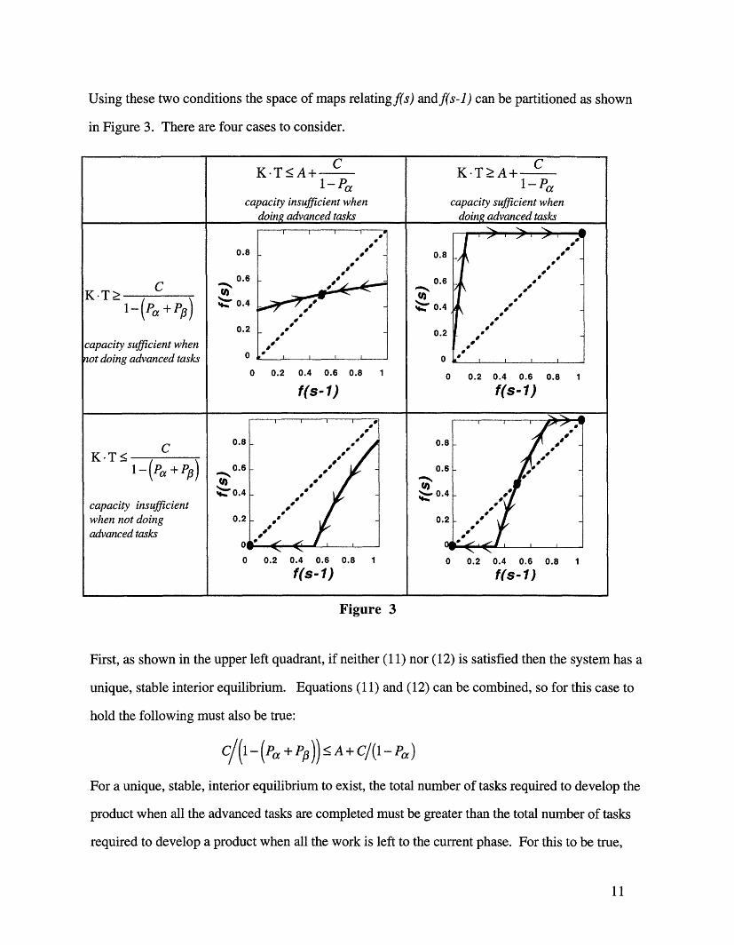
Using these two conditions the space of maps relatingf(s) andf(s-1) can be partitioned as shown

in Figure 3. There are four cases to consider.

> C1-(P +Pp

capacity sufficient when,ot doing advanced tasks

K.-T<>-(Pa +Pp)

capacity insufficientwhen not doingadvanced tasks

K.T<A+ 1-P a

capacity insufficient whendoine advanced tasks

0.8

0.6

U)t 0.4

0.2

0

0 0.2 0.4 0.6 0.8 1

f(s-1)

0 0.2 0.4 0.6 0.8 1

f(s-1)

K-T>A+ 1 - Pa

capacity sufficient whendoing advanced tasks

0.8

0.6

U)

0.4

0.2

0

0

0.

0.

U)" 0.

0o.

0.2 0.4 0.6 0.8

f(s-1)

0 0.2 0.4 0.6 0.8

f(s-1)

Figure 3

First, as shown in the upper left quadrant, if neither (11) nor (12) is satisfied then the system has a

unique, stable interior equilibrium. Equations (11) and (12) can be combined, so for this case to

hold the following must also be true:

/( - (P + Pp))< A + C/(1- P)

For a unique, stable, interior equilibrium to exist, the total number of tasks required to develop the

product when all the advanced tasks are completed must be greater than the total number of tasks

required to develop a product when all the work is left to the current phase. For this to be true,

11

I I I

0°

- 00

I

0

t_ II

- dP

- 0 >0

I00

0

00

0

00

0

I I I

8 - 0 -

6 4

4 000

02 - -

0/ 0

1

1

I1 II_1

_ _

l

advanced tasks must require more resources to complete than they save via the reduced defect

fraction. This situation occurs only when advanced tasks are not economical. Thus although the

model indicates that some advanced work is accomplished, the organization would be better off

ignoring it and doing more current tasks.

Second, as shown in the upper right quadrant, if (11) is satisfied and (12) is not, then the system

has one stable equilibrium atf*(s)=l. This case indicates that for the system to have a unique

equilibrium in which all advanced tasks are completed, total capacity, KT, must be greater than the

workload regardless of whether or not advanced tasks are completed. Thus, the only way to

eliminate the possibility that the system might settle into a regime in which advanced tasks are not

completed is to set resources at such a level that there is no benefit from doing those tasks.

Third, as shown in the lower left corner, if (12) is satisfied and (11) is not then the system has one

equilibrium atf*(s)=O. In this case resources are insufficient to support development regardless

of whether or not advanced work is completed. This suggests the fairly intuitive result that when

resources are over-utilized, performance will always tend towards the lower limit and, absent an

additional intervention, it is impossible for the system to operate at the desired equilibrium in

steady state. Under these conditions improvement efforts focused on up-front activities are

doomed to failure. Thus, a necessary condition for moving to a process with a significant amount

of up-front work is that sufficient resources be available to do that work. Empirical data suggests

that this case is more likely to occur than the previous one. For example Wheelwright and Clark

(1992) report that most of the firms they studied had, on average, twice as many projects in

progress as they had resources to complete them.

Fourth, as shown in the lower right quadrant, if both (1 1) and (12) are satisfied then the system

has three equilibria, two are stable and one is unstable. In contrast to the first case, if both (11)

and (12) hold then the following must also be true:

12

C CA+ < (13)

'-Pa -(P)+Pp)

Case number four requires that capacity be sufficient to support complete development when all

advanced tasks are done, but insufficient when the advanced work is not completed.

Thus, if (1) advanced tasks save more resources than they consume, and (2) resources are not

sufficient to support development when advanced work is completely ignored, then only two cases

are possible. Either resources are totally insufficient and the system will always tend towards a

minimum performance level, or the system has multiple equilibria. The stable equilibria occur at

f*(s)=l andf*(s)=O while the unstable equilibrium is at an interior point.

The existence of the unstable equilibrium underlies the core insight of this study: when conditions

(11), (12), and (13) are satisfied, the positive feedback loop dominates the behavior of this system

and drives it to one of the two stable equilibria. The dominance of this loop implies that the

system will display one of two behavior modes. The loop can work in the virtuous direction-

more advanced tasks completed, a lower defect rate, more resources dedicated to advanced tasks-

and drive the system towards the desirable equilibrium atf*(s)=l and the maximum performance

level. Or the loop can work in a vicious direction-fewer advanced tasks completed, a higher defect

rate, fewer resources dedicated to advanced tasks-and drive the system towards the undesirable

equilibrium atft(s)=O and a low performance level.

The location of the unstable equilibrium determines which of these two behaviors will prevail. It

represents the point at which the system begins to tilt one way or the other. The unstable

equilibrium is a bifurcation point in this system: if the system starts at any point below the unstable

equilibrium, then it will moved towards f(s)=O, and if the system starts from any point above the

unstable equilibrium, then it will moved towardsf*(s)=l.

13

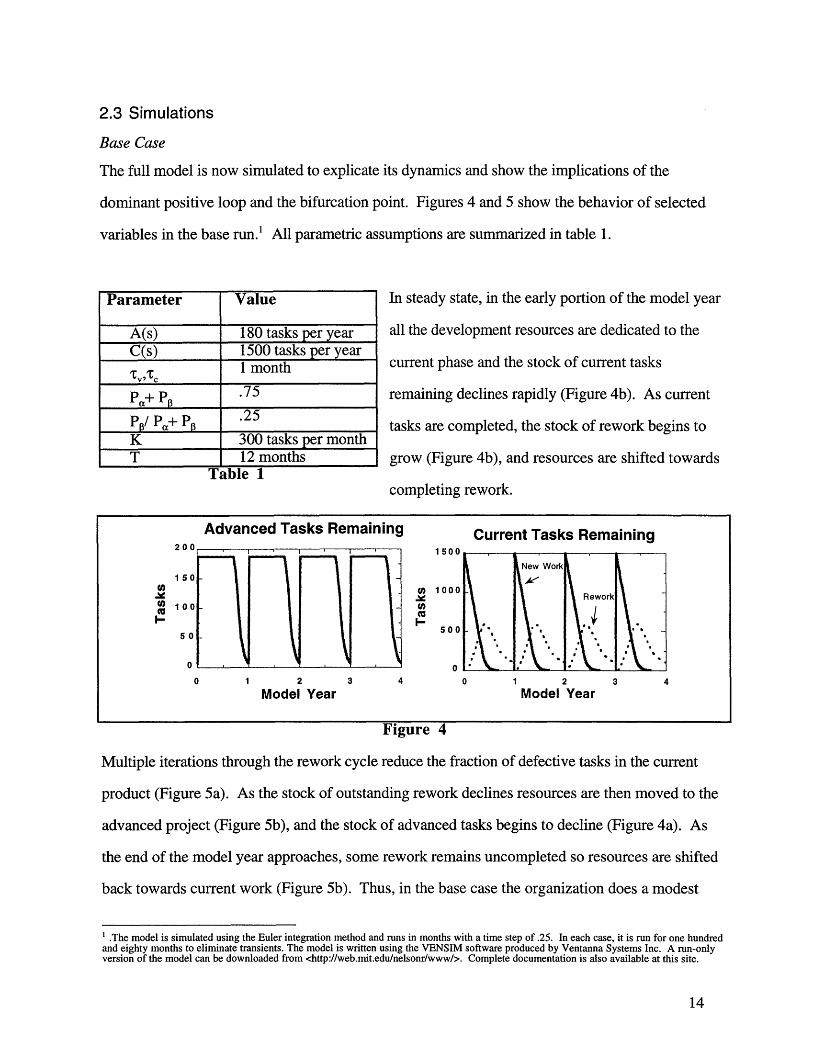
2.3 Simulations

Base Case

The full model is now simulated to explicate its dynamics and show the implications of the

dominant positive loop and the bifurcation point. Figures 4 and 5 show the behavior of selected

variables in the base run.' All parametric assumptions are summarized in table 1.

Parameter Value

A(s) 180 tasks per yearC(s) 1500 tasks per year

1 month

P, P .75

/ Pa+ PI .25K 300 tasks per monthT 12 months

Table 1

Advanced Tasks Remaining200

150

1005 0I

50

0

0 1 2

Model Year

In steady state, in the early portion of the model year

all the development resources are dedicated to the

current phase and the stock of current tasks

remaining declines rapidly (Figure 4b). As current

tasks are completed, the stock of rework begins to

grow (Figure 4b), and resources are shifted towards

completing rework.

Current Tasks Remaining

) 1

co

3 4 0 1 2Model Year

3 4

Figure 4

Multiple iterations through the rework cycle reduce the fraction of defective tasks in the current

product (Figure 5a). As the stock of outstanding rework declines resources are then moved to the

advanced project (Figure 5b), and the stock of advanced tasks begins to decline (Figure 4a). As

the end of the model year approaches, some rework remains uncompleted so resources are shifted

back towards current work (Figure 5b). Thus, in the base case the organization does a modest

.The model is simulated using the Euler integration method and runs in months with a time step of .25. In each case, it is run for one hundredand eighty months to eliminate transients. The model is written using the VENSIM software produced by Ventanna Systems Inc. A run-onlyversion of the model can be downloaded from <http://web.mit.edu/nelsonr/www/>. Complete documentation is also available at this site.

14

I I IJ

amount of 'fire fighting'. In the last month of the model year almost all the resources are focused

on improving the quality of the product in the current phase.

Fraction of Current Tasks Defective Fraction of Resources to Current Work

0a °.S > a 0.75 E0

0 2 3 40 2 3 4

Model Year Model Year

Figure 5

The base case depicts an organization that uses a relatively small set of up-front tools, but does

have a sufficient amount of resources to complete those advanced tasks it undertakes.

Transient Response

An instructive test of the model's behavior is to introduce a one-time increase in the amount of

development work. In the two new simulations shown below, in model year one, the number of

tasks required per project is increased by 20% and 25% respectively and then, in subsequent model

years, returned to the base level.

% of Advanced Work Completed Quality of Finished Design1.0 .5

X - 0 25% increase ................Base Case

0. 20% increase 0.25 20% increaseE 0.

25% increase

Base Case0 , I - -6..., ...... ... 0 - I

0 2 4 6 8 10 0 2 4 6 8 10Model Year Model Year

Figure 6

In the first model year after the increase the additional work reduces the fraction of advanced work

completed (Figure 6a). This leads to an increase in the defect rate for current work (Figure 7a) and

15

additional rework (Figure 7b). The 20% change prevents the advanced task completion fraction

from returning to its pre-pulse level, but it does increase over the previous year (Figure 7a).

% of Current Tasks Defective Rework to be Completed1.0 1000

25% increase 20% increase 25% increase20% increase Base

-OR sase

0 I C a s e

, .

0 1 2 3 4 5 6 7 0 1 2 3 4 5 6 7

Model Year Model Year

Figure 7

The increased completion fraction means the defect rate begins to decline, the resources required

for rework in subsequent years decline, and the completion fraction increases further. In this case,

the positive loop works in a virtuous direction and drives the system back to the initial equilibrium

and performance level (Figure 6b).

In contrast, the 25% increase shows different behavior. Due to the larger pulse, the initial decline

in the advanced completion fraction is greater (Figure 6a). The larger decline leads to a higher

defect rate for subsequent current work (Figure 7a), and creates additional rework (Figure 7b).

Critically, in contrast to the previous case, the growth in the resources required for rework is large

enough to cause the completion fraction to decline further in subsequent model years rather than

begin to recover as in the previous case (Figure 6a). Here the positive loop works in a vicious

direction and drives the system away from the initial, desirable equilibrium, towards the

undesirable one and causes a significant deterioration in performance (Figure 6b).

In the second case a temporary change in workload, the pulse, causes a permanent decline in

performance. The change only occurs in the second test because only in this case is the pulse large

enough to move the system beyond the bifurcation point and cause the dominant feedback loop to

work in the opposite direction. Figure 8 gives another view of the bifurcation point.

16

0

0.375 a

co0

.25

0.125

a

0.3

Pulse

Figure 8

The figure was generated by running the model for a range of pulse sizes and plotting the response

surface. The surface shows how the positive feedback loop creates a system with the potential to

operate at multiple equilibria and a system that can show dramatic changes in performance initiated

by small changes in inputs. At pulse sizes of less than 20% of the base level the system is robust

to perturbation. As the pulse size grows above 20%, however, the system's ability to recover is

lost. The change occurs because at that point, the dominant positive loop begins to work in the

opposite direction and drives the system to a different equilibrium.

3. Introducing New Up-front ToolsSo far the analysis suggests that, under the conditions outlined above, product development

systems can have multiple steady state equilibria and a temporary external shock can cause a

permanent change in performance. In this section, the response of the system to the introduction

of new development tools is analyzed.

17

0.5

v

3.1 Model StructureThe model developed so far is based on the assumption that the defect fraction, PD, is divided into

two fixed components, P,, the fraction of defects that cannot be eliminated by advanced tasks, and,

Pp, the fraction that can. The introduction of additional development tools is modeled by making

these two parameters variable and assuming that they are determined by the size of the set of tools

currently in use. The introduction of a new set of tools means that A, the set of up-front activities,

is increased. So in the year of introduction, A is increased from A' to A2 (A 2DA'). The cost of

introducing new tools is captured by the fact that A is now larger and thus requires more resources.

The benefit of the new tools is captured by changes in Pa and P. Specifically, the sum of P, and

Pp is assumed to be constant, Pa+P,=Pm and the split between the two probabilities is determined

by the variable w(s):

P(s) =P x.(1 -w(s))

Ps)=P w(s)

w(s) captures the organization's current ability to use the tools it has at its disposal and is

determined by the following equations:

w(s)=y-w(s-1)+(1-y)z(s), Y E [0,1]

Z() = z(s-1)+(1- ) ( Amax A ' [0,1]

(14)

(15)

(16)

(17)

w(s), the organization's current ability, is a moving average of z(s), the organization's current

knowledge of the tools. Equation (16) captures that fact that, once a tool is learned, time is

required to develop experience before it can be used effectively. 1/y represents the average time

required to gain such experience and is assumed to be one and one half model years.

18

z(s) is determined by AC(s, T)/A m where A"' is the maximum available set of tools and

Ac(s, T)/Ama represents that fraction of that set used in year s. To capture the delays inherent in

learning how to use new tools, z(s) is assumed to be a weighted average of that fraction where 1/k

represents the average learning delay (assumed to be one and one half model years). Thus, if the

feasible set of tools is increased, the organization does not immediately benefit from using them.

Instead time is required to learn the new tools and develop the appropriate skill.

3.2 Simulations

Figures 9 and 10 show two simulations in which new tools are introduced. In the base case the

firm is assumed to use only 25% of the available tools, but at 100% effectiveness

(A 1/Ama=w(s)=.25). In the first simulation, in model year one, the set of tools is doubled so that

A2/Amax=.5. In the second, the set of tools is increased to the maximum level so A2 /Ama =1.

% of Advanced Work Completed Experience with Advanced Tools1.0 1.0

0 Base Case 0) Z 50% Introduction7 0. 5 A 50% Introduction O 100% IntroductionE ..0.5.........

W. Base Case100% Introduction

0 0

0 2 4 6 8 10 0 2 4 6 8 10Model Year Model Year

Figure 9

In both cases, due to the initial increase in the number of advanced tasks, the fraction of advanced

work completed declines (Figure 9a). In the case of a 50% introduction, the initial decrease is

small and insufficient to initiate the downward spiral. Further, since the fraction of advanced work

stays high, experience with the tools, represented by w(s), begins to increase (figure 9b), and the

fraction of defects that can be eliminated by advanced work increases. The increase in Pp makes the

dominant positive loop stronger, further speeding the virtuous cycle that drives the system towards

19

f*(s)=1. The steady state performance of the model is improved as the additional tools enable a

larger fraction of defects to be eliminated (Figure 10).

Quality of Finished Design.Q5 t o F ini , I In contrast, although the second simulation is identical

100% Introduction - ------.' to the first in every respect except that more tools are

0 0.2 5 Base Case' introduced, the results are quite different. The more

OR ' ° "- 50% Introduction ambitious change in the process causes a larger initial

0 2 4 6 8 10 decline in the advanced task completion fractionModel Year

(Figure 9a), a greater defect probability in current

Figure 10 tasks, and a further reduction in the completion

fraction. Initially experience with the new tools begins to rise making current work more

productive (Figure 9b), but the growth is more than offset by the decline in the advanced task

completion rate. As the rate of advanced task completion declines, with a delay, experience with

and knowledge about the tools also begins to decline. The downward spiral continues until the

model reaches the undesirable equilibrium with little advanced work being accomplished and a

substantial decline in steady state performance (Figure 10). The cause of the decline is the

introduction of a tool set sufficiently large that the initial cost of learning moves the system past the

bifurcation point. Once beyond the bifurcation point, the positive loop progressively reduces the

amount of advanced work completed in each subsequent model year, increasing the current work

defect fraction and reducing the levels of knowledge and experience. Figure 11 shows the

response surface for a range of introduction strategies.

The figure shows how the dominant positive loop creates a highly non-linear response to the

introduction of additional up-front activities. As the size of the set of tools introduced increases,

steady state performance also improves until the bifurcation point is reached. Beyond an

introduction level of 40%, the loop operates in the opposite direction and pushes the system

towards the undesirable equilibrium. Thus, although the tools would unequivocally help the

20

organization if the appropriate knowledge and experience were developed, their introduction has

the potential to make the system's performance worse rather than better.

Figure 11

4. Policies for System Improvement4.1 Aggregate Resource Planning

In this section policy changes that might improve performance are discussed. The most obvious of

these is to closely match the workload with the available resources. This does not constitute a

particularly novel insight and this is not the first study to suggest that overloading a development

system hurts performance. Wheelwright and Clark (1992) describe the 'canary cage' problem: too

many birds in a cage reduce the available resources, food, water, and space, and none of the

animals thrive. Similarly, in product development, they argue, too many projects leads to a poor

allocation of resources and mediocre products. The rule implicit in the 'canary cage' metaphor is

even allocation across all projects and, as a consequence, the dynamics around projects in different

phases of development are not discussed. Thus, they reach the conclusion suggested by case

number three in section 2.2: if resources are insufficient, even when the process is executed

21

0.5-

(0 0.40

a:> 0.300

o a 0.:O.- O .

0.

o

).75

0

2o °' 00 ,-

---~~~~~~~~~~~~~~~~~~~~~~

I I1

correctly, then performance will tend towards the minimum level and 'fire fighting' dynamics will

ensue. The model presented here extends this argument and yields two additional conclusions.

First, the analysis shows that an organization may have sufficient resources to execute the process

correctly for all projects, but could still be stuck at the undesirable equilibrium. Thus, when doing

resource planning it is critical to assess the resource requirements for projects given the current

state of the development process, not that which would be required were the process operating as

desired. To move a system out of the undesirable equilibrium, the number of projects in progress

may need to be reduced until the balance between advanced and current work is improved.

This dynamic can be worse when a change effort is underway. A failure mode observed in a large

scale product development improvement effort studied in Repenning and Sterman (1997) was the

allocation of resources under the assumption that the new process was already in place and

operating at full capability. This rule was not inadvertent, but an explicit part of the improvement

strategy under the rationale that if the resources were removed participants would have no choice

but to follow the process to get their work done. The flaw in this logic is that there were already

projects in progress that had not been done using the new process and thus required more

resources than the new process dictated. The ensuing scarcity initiated the downward spiral and

caused a significant decline in capability and the failure of the initiative.

Second, the analysis highlights the role of variability and unpredictability: even if the system

operates at the desired state, variations in the workload, if they push the system beyond the

bifurcation point, can initiate the downward spiral and drive the system to a low performance level.

It is easy to show that the location of the bifurcation point (the unstable equilibrium) is determined

by resource utilization; as the resource level is increased, the bifurcation point moves closer to the

equilibrium atf*(s)=O, and a larger shock is required to move the system to the undesirable

equilibrium. In fact, if resources are sufficiently increased the undesirable equilibrium disappears

22

altogether (case number two from section 2.2). Such a policy, however, requires that the system

is only loaded to the point where projects can be completed without advanced work, thus nullifying

any savings generated by the introduction of those activities. Thus, there is a direct trade-off

between the robustness to tilting and steady state performance. Resource plans need to account for

the uncertainty in the estimated requirements.

As important as is good resource planning, estimating project requirements and quantifying the

remaining uncertainty is difficult. The difficulty is further compounded if the effectiveness of the

process is changing due to ongoing improvement activity. Thus, although good resource planning

is important, the difficulty of doing it precisely suggests that it is valuable to consider other

complementary options. In the rest of this section another policy is investigated, one that can make

the system more robust to errors in resource planning.

4.2 Limiting Strategies

The policy analyzed here is based on the idea that an organization often has a number of ways to

compensate for low process capability including fixing defects as they occur and investing in long

run improvements that eliminate those defects in the first place (the classic prevention/correction

distinction). Frequently both paths cannot be pursued simultaneously and the organization must

allocate scarce resources between fixing current problems and preventing future ones. Repenning

and Sterman (1997) discuss in detail why there is a strong bias in many organizations towards

correction and away from prevention. To counteract this bias, Repenning (in progress) introduces

the concept of limiting strategies. Limiting strategies are based on the idea that effective

implementation of new improvement methods focused on prevention requires eliminating the

organization's ability to use short-cut correction methods. The archetypal example of such a

strategy is the use of inventory reduction to drive fundamental improvements in machine up-time

and yield in manufacturing operations. As the amount of material released to the production

system is reduced, operators and supervisors are less able to compensate for low yield and up-time

23

by running machines longer and holdinthe only

Way to meet production objectives is through fundamentalimprovemens.

The first step in Using a limitig strategy is to identiy the key mechanisms through hich theorganiza n COmpensate for low rocess capability , In product development systemsone ay toCOmpensate for low capability is to redo existing ork to correct defets. In the model, this isrepresented by multiple iterations through the re-work cycl .To use mdel thau cction f resurcek m ust be ts a ing strategy theallocation of to re-work ust be constrained. In the model this is implementesimple fashion. During the current phase a design freeze is introduced and, from that date

forward, no resources are allocated to re-work. at

Workload Variaions Under Limitation

Figure 1 shows e response when theFigure 12 shows the response When these s system is again subjected to pulses of various Sizes. The

only difference between these simulations and those Used to generate Figure 8 is that a designfreeze has been introduced with one month rems.ning tho

,,~ m on t iihr- Figure 8 is that a design

24

v

The surface shows that the system's robustness to pulse inputs is greatly increased under the freeze

policy. Larger pulses cause larger increases in the defect fraction, but in all cases the change is

temporary. The policy works because it weakens the positive feedback loop responsible for the

undesirable behavior. Figure 13 shows the phase plot for the system when the freeze policy is in

place. The freeze policy eliminates the equilibrium atf*(s)=O by insuring that some advanced

work gets done each period.

0.8 13

'+. 0.4 _

0.2 ,"

0 I

0 0.2 0.4 0.6 0.8 1

f(s-1)Figure 13

Although the policy is effective in increasing the

robustness of the system to variation in workload, it is

not free. In the new, freeze-date equilibrium, the fraction

of released product that is defective is now higher.

The Introduction of New Tools with Limitation

The freeze policy has a more dramatic impact when coupled with the introduction of additional

tools. Recall from section three that if capacity is insufficient and too large a set of tools is

introduced, the tilting dynamic can be initiated. Figure 14 shows this simulation along with

another experiment in which the freeze policy is in place.

% of Advanced Work Completed Quality of Finished Design1.0 ---- .

_t ' Base Case 0 100% IntroductionBase Case without Freeze /

V. ' =0. 5 \ *. , 100% Introduction 4)0.25 - Base Case

o with Freeze

o 100% Introduction 100% Introduction6 fi ^ without freeze

0 0 with Freeze" 0 'I

0 2 4 6 8 10 0 2 4 6 8 10Model Year Model Year

Figure 14

25

As in the previous case, the introduction of the new tools causes a decline in the fraction of

advanced work that is completed. However, with the freeze date in place, the decline is only

temporary and, with time, the fraction recovers. Similarly, the defect fraction initially rises and

only declines after a number of model years. The length of the transient depends on the learning

delay, here assumed to be three model years. The freeze policy eliminates the undesirable

equilibrium, but as in the previous case, the policy is not free. The steady state performance of this

system prior to the introduction of the new tools is lower with the freeze policy in place. Figure 15

shows the surface plot for the range of tool introductions with the freeze policy in place.

I I

Figure 15

5. Discussion and Conclusion5.1 From Robust Product Design to Robust Process Design

It has become an article of faith among business writers that managers should focus on whole

systems and processes, not specific pieces and functions (Garvin 1998, Senge 1990, Stata 1989),

and many authors have recognized that managers who treat development projects as independent

entities do so at their peril (e.g. Wheelwright and Clark 1992, 1995 and Zangwill 1995). The

model presented here shows one example of how a system-level perspective leads to insights that

26

0.5-

0.4a00 0.

00.

I 0.

0.7.75

)a

;o

P.

20

could not be gained if the focus was restricted to an individual project. These insights have a

number of implications for both managers and researchers which have already been discussed.

There is, however, a larger message for both the academic and practitioner communities. Decision

making processes are the major focus of much of the literature on managing product development.

This study has tried to demonstrate that the behavior of product development systems is influenced

in important ways by positive feedback loops and time delays, two elements that comprise complex

dynamic systems (Sterman 1994). Unfortunately, experimental research on human decision

making in such contexts shows that people perform very poorly when trying to manage dynamic

systems of even modest complexity (Sterman 1989a, 1989b; Brehmer 1992; Funke 1991), and that

very little learning occurs in such environments (Paich and Sterman 1993, Diehl and Sterman

1995). Thus any effort to influence the day-to-day decision processes of managers in complicated,

dynamic environments faces a difficult challenge.

As a consequence, an alternative and complementary approach to influencing such systems may be

in order. Specifically, this study suggests that changes to the structure of the process may have

more leverage than improving the quality of decisions made within that structure. To use an

analogy from product engineering, a major insight underlying robust design methods is that it is

often more productive to change a product's design to make it more robust to variability in the

dimensions of its constituent components than to reduce the variability of the on-going

manufacturing processes that create those components. Similarly, in some cases it may be more

effective to create a development process that is robust to variations in the quality of decision

making rather than to try to improve that quality.

For example, the analysis suggests that improving managers' ability to estimate resource

requirements accurately can enhance the system's performance Unfortunately, there are a host of

reasons why these estimates are difficult to make. First, as mentioned previously, under any

27

circumstances estimating the capacity of a product development system can be very difficult and

imprecise. Second, absent an accurate estimate, managers are often tempted to overload

development systems to insure that resources are fully utilized. Third, the conditions in such

systems are very poor for learning (Sterman 1994), and may, in many cases, teach managers

exactly the wrong lessons (Repenning and Sterman 1997).

A complementary approach to improvement is to focus not on the decisions, but on the structure of

the process itself. In the model presented here, a policy of fixing a portion of the resource

allocation, rather than leaving it to the discretion of managers, is a simple solution that greatly

increases the robustness of the process to variations in workload. The policy can also dramatically

improve the chance that a new tool will be successfully adopted.

Thus, the study suggests that a core idea of robust design is potentially applicable to the design of

processes and organizations. There are, however, two very important differences. First, in robust

product design the variability is physical in nature and its causes well understood. In designing

robust processes, the variability is primarily behavioral. Existing research on decision making in

dynamic environments should inform new designs of product development processes, and more

research is needed on how people behave in such environments.

Second, it can be prohibitively costly to run the needed experiments in actual organizations and,

unlike in product development, prototyping is often not an option. Thus, the development of

formal models that accurately capture the dynamics of such processes is critical to understanding

which policies are robust to behavioral variation. The methodology used here as well as many

others can provide the means to generate useful models of organizations and processes focused on

improving their design. Simulation has been used successfully to improve the performance of a

wide range of business systems including preventive maintenance programs (Carroll, Markus and

Sterman 1997), process improvement programs in manufacturing (Sterman, Repenning and

28

Kofman 1997, Repenning 1997b), and large-scale project management (Cooper 1980, Abdel-

Hamid and Madnick 1991).

5.2 Future Work

The model could be profitably extended in a number of directions. In the interest of simplicity a

number of assumptions have been made that could be relaxed. Foremost among these is the fixed

product introduction date. This assumption is a good approximation to the actual practice in some

industries, such as automotive manufacturing, but not others. In many cases the introduction date

can be postponed until the product achieves a desired performance level. Some form of the tilting

dynamic could still be present in these situations. Typically a product plan is established that

outlines future development projects for an extended period of time. Tilting could occur in this

type of system if, when one of these projects is completed after the planned date, the completion

dates for subsequent projects are not updated to reflect the change. It seems plausible that in such

systems people might try to 'catch-up' on subsequent projects, and do so by ignoring up-front

activities. If so, then the same results discussed here might apply. Verifying that this is in fact the

case, however, remains for future work.

Alternatively, there are also additional insights that might be obtained within the existing model

structure but with new modes of analysis, mainly optimization. Two important trade-offs have

been identified, but no attempt made to calculate their optimal resolution. First, the analysis shows

a trade-off between steady-state performance and robustness to variability. Second, it also shows

a trade-off between the size of the set of tools introduced and the resulting worse-before-better

behavior (under the freeze policy). Additional insight may result from analyzing this in more

detail. More generally, the analysis suggests that the sequence and timing of tool introduction

matters. In an expanded framework that captures a more heterogeneous set of tools, optimally

calculating the sequence and timing of introduction may yield valuable insight.

29

6. ReferencesAbdel-Hamid, T. and S. Madnick (1991). Software Project Dynamics: an integrated approach,

Englewood NJ, Prentice Hall.

Adler, P.S., A. Mandelbaum, V. Nguyen and E. Schwerer (1995). From product to processmanagement: an empirically-based framework for analyzing product development time,Management Science, 41, 3:458-484.

Brehmer, B., (1992). Dynamic Decision Making: Human Control of Complex Systems, ActaPsychologica, 81, 211-241.

Carroll, J., J. Sterman, and A. Markus (1997). Playing the Maintenance Game: How MentalModels Drive Organization Decisions. R. Stern and J. Halpern (eds.) Debating Rationality:Nonrational Elements of Organizational Decision Making. Ithaca, NY, ILR Press.

Clark, K. and T. Fujimoto (1991). Product Development Performance: Strategy, Organizations,and Management, Boston, MA, HBS Press.

Cooper, K (1980). Naval Ship Production: A Claim Settled and a Framework Built,INTERFACES, 10, 6.

Diehl, E. and J.D. Sterman (1995). Effects of Feedback Complexity on Dynamic DecisionMaking, Organizational Behavior and Human Decision Processes, 62(2): 198-215.

Dertouszos, M., R. Lester, and R. Solow (1989). Made in America: Regaining the ProductiveEdge, The MIT Press, Cambridge, MA.

Eppinger, S.D, M.V. Nukala and D.E. Whitney (1997). Generalized Models of Design IterationUsing Signal Flow Graphs, Research in Engineering Design, 9: 112-123.

Funke, J. (1991). Solving Complex Problems: Exploration and Control of Complex Systems, inR. Sternberg and P. Frensch (eds.), Complex Problem Solving: Principles andMechanisms. Hillsdale, NJ: Lawrence Erlbaum Associates.

Garvin, D.A. (1998). The Processes of Organization and Management, Sloan ManagementReview, 39,4:33-50.

Huber, G.P. and W.H. Glick (1993), Organizational Change and Redesign: Ideas and InsightsforImproving Performance. New York, Oxford University Press.

Jones, A.P. and N. P. Repenning (1997). Sustaining Process Improvement at Harley-Davidson.Case Study available from second author, MIT Sloan School of Management, Cambridge,MA 02142.

Kanter, R.M., T.D. Jick, and R. A. Stein (1992). The Challenge of Organizational Change. NewYork, Free Press

Krahmer, E. & R. Oliva (1996). A Dynamic Theory of Sustaining Process Improvement Teams inProduct Development., in Beyerlein, M. and D Johnson (eds), Advances inInterdisciplinary Studies of Teams, Greenwhich, CT, JAI Press..

Paich, M. and Sterman, J. (1993). Boom, Bust, and Failures to Learn in Experimental Markets.Management Science, 39(12), 1439-1458.

Plous, S. (1993). The Psychology of Judgment and Decision Making, New York, McGraw-Hill.

Repenning, N. (in progress). Improvisational Change, Process Improvement, and LimitingStrategies. Working Paper Available from author, Sloan School of Management, MIT,Cambridge, MA 02142.

30

Repenning N. and J. Sterman (1997). Getting Quality the Old-Fashion Way: Self-ConfirmingAttributions in the Dynamics of Process Improvement, to appear in Improving Research inTotal Quality Management, National Research Council Volume, Richard Scott and RobertCole, eds.

Repenning, N. (1997a). Resource Dependence in Product Development Improvement Efforts.working paper available from the author, MIT Sloan School of Management, CambridgeMA 02142.

Repenning, N. (1997b). Successful Change Sometimes Ends with Results. working paperavailable from the author, MIT Sloan School of Management, Cambridge MA 02142.

Repenning, N. (1996). Reducing Product Development Time at Ford Electronics, Case Studyavailable from author, MIT Sloan School of Management, Cambridge MA 02142.

Senge, P. (1990). The Fifth Discipline: The Art and Practice of the Learning Organizations,Doubleday, New York, NY.

Stata, R. (1989). Organizational Learning: The Key to Management Innovation, SloanManagement Review, 30(3), Spring, 63-74.

Sterman, J.D. (1994). Learning in and about complex systems, System Dynamics Review,10,3:291-332.

Sterman, J. D. (1989a). Misperceptions of Feedback in Dynamic Decision Making. OrganizationalBehavior and Human Decision Processes 43 (3): 301-335.

Sterman, J. D. (1989b). Modeling Managerial Behavior: Misperceptions of Feedback in a DynamicDecision Making Experiment. Management Science 35 (3): 321-339.

Sterman, J., N. Repenning, and F. Kofman (1997). Unanticipated Side Effects of SuccessfulQuality Programs: Exploring a Paradox of Organizational Improvement. ManagementScience, April, 503-521.

Van de Ven, A., and M.S. Poole (1995). Explaining Development and Change and Organizations,Academy of Management Review, Vol. 20, No. 3, 510-540

Wheelwright, S. and K. Clark (1992). Revolutionizing Product Development: Quantum Leaps inSpeed Efficiency and Quality, The Free Press, New York, NY.

Wheelwright, S. and K. Clark (1995). Leading Product Development, The Free Press, New York,NY.

Ulrich, K. and S. Eppinger (1995). Product Design and Development, McGraw-Hill Inc., NewYork, NY.

Zangwill, W. (1993). Lightning Strategies for Innovation: how the world's best create newprojects, Lexington Books, New Your, NY.

31

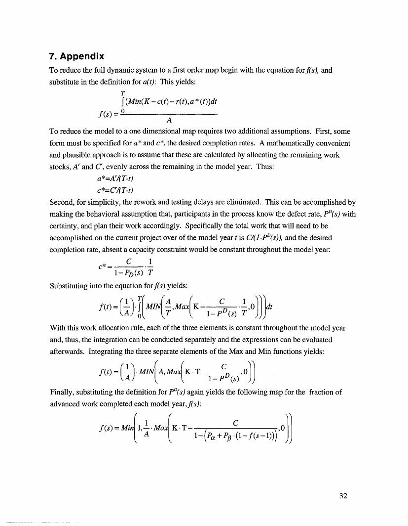
7. AppendixTo reduce the full dynamic system to a first order map begin with the equation forf(s), and

substitute in the definition for a(t): This yields:

T

J(Min(K - c(t) - r(t),a * (t))dt

f(s) = 0A

To reduce the model to a one dimensional map requires two additional assumptions. First, some

form must be specified for a* and c*, the desired completion rates. A mathematically convenient

and plausible approach is to assume that these are calculated by allocating the remaining work

stocks, A r and C, evenly across the remaining in the model year. Thus:

a*=Ar/(T-t)

c*=C/(T-t)

Second, for simplicity, the rework and testing delays are eliminated. This can be accomplished by

making the behavioral assumption that, participants in the process know the defect rate, P°(s) with

certainty, and plan their work accordingly. Specifically the total work that will need to be

accomplished on the current project over of the model year t is C/(1-PD(s)), and the desired

completion rate, absent a capacity constraint would be constant throughout the model year:

C 11 -PD(s) T

Substituting into the equation forf(s) yields:

(A JMIN T , Max K - pD(s) T O))jdt

With this work allocation rule, each of the three elements is constant throughout the model year

and, thus, the integration can be conducted separately and the expressions can be evaluated

afterwards. Integrating the three separate elements of the Max and Min functions yields:

f(t) = 1 MINjA,MaxK. T- -D 0A \LI-(A~i · ··i 1- PD(s)

Finally, substituting the definition for PD(s) again yields the following map for the fraction of

advanced work completed each model year,f(s):

f(s)=Min 1, -MaxK T - C !oA 1-(Pa + Pp (1 - f(s - 1))) '

32