The Transition of Corruption: From Poverty to Honesty

The transition of corruption: From poverty to honesty by Erich Gundlach and Martin Paldam

No. 1411| March, 2008

Kiel Institute for the World Economy, Düsternbrooker Weg 120, 24105 Kiel, Germany

Kiel Working Paper No. 1411| March, 2008

The transition of corruption:

From poverty to honesty

Erich Gundlach and Martin Paldam

Abstract: Measures of corruption and income are highly correlated across countries. We use prehistoric measures of biogeography as instruments for modern income levels. We find that our instrumented incomes explain the cross-country pattern of corruption just as well as do actual incomes. This result demonstrates that the long-run causality is entirely from income to corruption. Hence, there is a Corruption Transition: As countries get rich, corruption vanishes.

Keywords: Long-run development, corruption, biogeography

JEL classification: B25, O1

Erich Gundlach Kiel Institute for the World Economy 24100 Kiel, Germany Telephone: +49 431 8814 284 E-mail: [email protected]

Martin Paldam School of Economics and Management University of Aarhus DK-8000 Aarhus C Telephone: +45 8626 3140 E-mail: [email protected]

____________________________________ The responsibility for the contents of the working papers rests with the author, not the Institute. Since working papers are of a preliminary nature, it may be useful to contact the author of a particular working paper about results or caveats before referring to, or quoting, a paper. Any comments on working papers should be sent directly to the author. Coverphoto: uni_com on photocase.com

1. Introduction

Measures of corruption and income are highly correlated across countries, as shown by Table

1, but no agreement has been reached in the literature about the main direction of causality

between the two variables. Some (as Lambsdorff 2007) claim that corruption is a vice causing

low growth, so that causality is mainly from corruption to long-run income. Others (Treisman

2000; Paldam 2001, 2002) claim that corruption is a poverty driven disease that vanishes

when countries develop, so that causality is mainly from income to corruption.

The empirical problem is that the available series of corruption perceptions are still

rather short and they contain much autocorrelation. Hence it will take some time before they

permit formal time series tests of causality. We have summarized the empirical findings till

now in Paldam and Gundlach (2008), which also provides an informal causality analysis. This

informal test suggests that the relation between income and corruption is just another

transition that occurs when countries develop from poor to rich.1 The purpose of the present

paper is to provide a new formal test of the long-run direction of causality between income

and corruption. Our test is based on the present cross-country pattern (c-cp) of corruption and

income, and uses instrumental variables to identify the long-run direction of causality.

Given that all countries experienced fairly similar average income levels 200-500

years ago, modern income levels reveal cross-country differences in the long-run growth rate.

So regressing measures of corruption on levels of income will identify the long-run income

effect if the possible reverse causality from corruption to income can be controlled for. In

order to obtain a measure of corruption-free incomes, we explain the present c-cp of income

by a set of extreme instruments that refer to prehistoric measures of biogeography. We then

show that these incomes explain the c-cp of corruption just as well as the actual c-cp of

incomes. It follows that all long-run causality is from income to corruption: hence there is a

Corruption Transition.

The paper proceeds as follows. Section 2 explains the logic of our test and presents the

main result. Section 3 discusses some robustness test, and Section 4 concludes. We are brief

since a parallel paper analyzing the relation between democracy and income (Gundlach and

Paldam 2008) provides a more detailed discussion of our empirical model and of the literature

that motivates our empirical strategy. All variables used are defined in the appendix. 1. We use the term Grand Transition for the set of transitions (the demographic, the urban, the democratic, etc.), which together constitute development, see Paldam and Gundlach (2008).

2

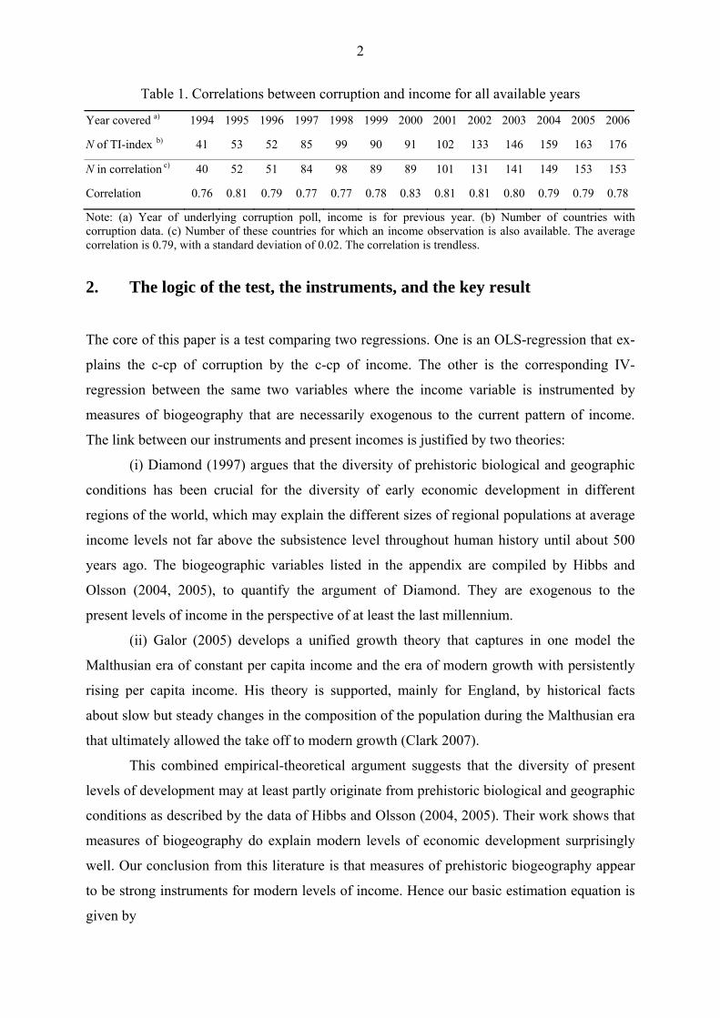
Table 1. Correlations between corruption and income for all available years

Year covered a) 1994 1995 1996 1997 1998 1999 2000 2001 2002 2003 2004 2005 2006

N of TI-index b) 41 53 52 85 99 90 91 102 133 146 159 163 176

N in correlation c) 40 52 51 84 98 89 89 101 131 141 149 153 153

Correlation 0.76 0.81 0.79 0.77 0.77 0.78 0.83 0.81 0.81 0.80 0.79 0.79 0.78

Note: (a) Year of underlying corruption poll, income is for previous year. (b) Number of countries with corruption data. (c) Number of these countries for which an income observation is also available. The average correlation is 0.79, with a standard deviation of 0.02. The correlation is trendless.

2. The logic of the test, the instruments, and the key result

The core of this paper is a test comparing two regressions. One is an OLS-regression that ex-

plains the c-cp of corruption by the c-cp of income. The other is the corresponding IV-

regression between the same two variables where the income variable is instrumented by

measures of biogeography that are necessarily exogenous to the current pattern of income.

The link between our instruments and present incomes is justified by two theories:

(i) Diamond (1997) argues that the diversity of prehistoric biological and geographic

conditions has been crucial for the diversity of early economic development in different

regions of the world, which may explain the different sizes of regional populations at average

income levels not far above the subsistence level throughout human history until about 500

years ago. The biogeographic variables listed in the appendix are compiled by Hibbs and

Olsson (2004, 2005), to quantify the argument of Diamond. They are exogenous to the

present levels of income in the perspective of at least the last millennium.

(ii) Galor (2005) develops a unified growth theory that captures in one model the

Malthusian era of constant per capita income and the era of modern growth with persistently

rising per capita income. His theory is supported, mainly for England, by historical facts

about slow but steady changes in the composition of the population during the Malthusian era

that ultimately allowed the take off to modern growth (Clark 2007).

This combined empirical-theoretical argument suggests that the diversity of present

levels of development may at least partly originate from prehistoric biological and geographic

conditions as described by the data of Hibbs and Olsson (2004, 2005). Their work shows that

measures of biogeography do explain modern levels of economic development surprisingly

well. Our conclusion from this literature is that measures of prehistoric biogeography appear

to be strong instruments for modern levels of income. Hence our basic estimation equation is

given by

3

, (1) iiii y εγβακ +Χ++= '

where iκ is the degree of corruption in country i, is the natural logarithm of GDP per

capita in constant international dollars, is a matrix of other covariates that may be

included,

iy

'iΧ

α is a regression constant, ε is an error term, and β is the coefficient of interest

that measures the long-run effect of income on corruption once income is appropriately

instrumented.

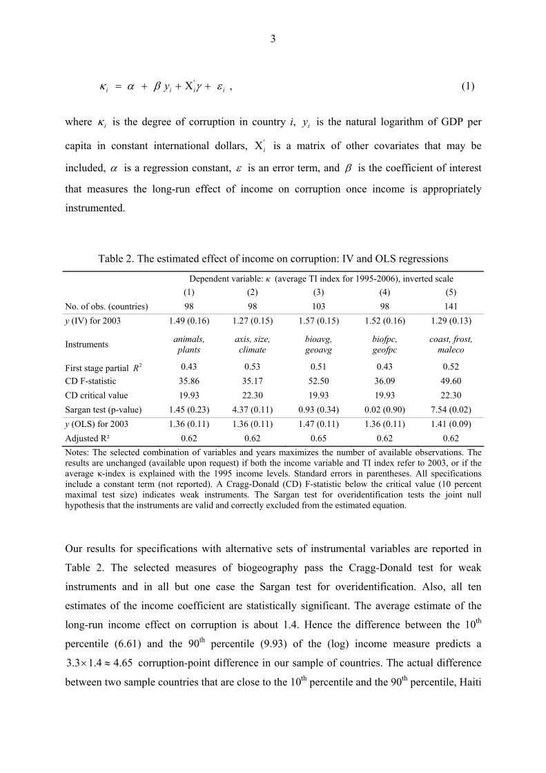
Table 2. The estimated effect of income on corruption: IV and OLS regressions

Dependent variable: κ (average TI index for 1995-2006), inverted scale (1) (2) (3) (4) (5) No. of obs. (countries) 98 98 103 98 141 y (IV) for 2003 1.49 (0.16) 1.27 (0.15) 1.57 (0.15) 1.52 (0.16) 1.29 (0.13)

Instruments animals, plants

axis, size, climate

bioavg, geoavg

biofpc, geofpc

coast, frost, maleco

First stage partial 2R 0.43 0.53 0.51 0.43 0.52 CD F-statistic 35.86 35.17 52.50 36.09 49.60 CD critical value 19.93 22.30 19.93 19.93 22.30 Sargan test (p-value) 1.45 (0.23) 4.37 (0.11) 0.93 (0.34) 0.02 (0.90) 7.54 (0.02) y (OLS) for 2003 1.36 (0.11) 1.36 (0.11) 1.47 (0.11) 1.36 (0.11) 1.41 (0.09) Adjusted R² 0.62 0.62 0.65 0.62 0.62 Notes: The selected combination of variables and years maximizes the number of available observations. The results are unchanged (available upon request) if both the income variable and TI index refer to 2003, or if the average κ-index is explained with the 1995 income levels. Standard errors in parentheses. All specifications include a constant term (not reported). A Cragg-Donald (CD) F-statistic below the critical value (10 percent maximal test size) indicates weak instruments. The Sargan test for overidentification tests the joint null hypothesis that the instruments are valid and correctly excluded from the estimated equation.

Our results for specifications with alternative sets of instrumental variables are reported in

Table 2. The selected measures of biogeography pass the Cragg-Donald test for weak

instruments and in all but one case the Sargan test for overidentification. Also, all ten

estimates of the income coefficient are statistically significant. The average estimate of the

long-run income effect on corruption is about 1.4. Hence the difference between the 10th

percentile (6.61) and the 90th percentile (9.93) of the (log) income measure predicts a

corruption-point difference in our sample of countries. The actual difference

between two sample countries that are close to the 10

65.44.13.3 ≈×th percentile and the 90th percentile, Haiti

4

and Finland, is 7.85 corruption points, so our estimate explains about 60 percent of the

observed difference in the corruption index of the two countries.

The key result from Table 2 is that the IV-results do not differ significantly from the

corresponding OLS-results in any of the five specifications, so there is obviously no upward

bias due to reverse causality. All five pairs of estimates suggest that the long run causality is

entirely from income to corruption. Our further results are based on the specification in

column (4), which uses our preferred instruments.

3. Robustness of the main result

One major objection to our main result in Table 2 is that our estimates are biased due to

omitted variables. We check the robustness of our estimate of the income effect by adding ten

control variables one by one to avoid multicollinearity. Our control variables are either socio-

political (Table 3) or ethno-cultural (Table 4). We speculate that these variables have an effect

on corruption which may either be independent of the income effect or may even dominate

the presumed income effect.2

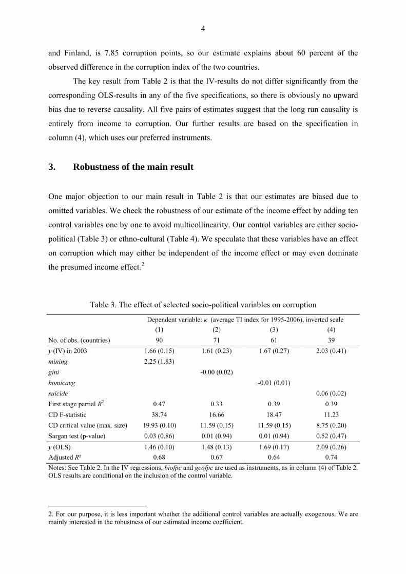
Table 3. The effect of selected socio-political variables on corruption

Dependent variable: κ (average TI index for 1995-2006), inverted scale (1) (2) (3) (4) No. of obs. (countries) 90 71 61 39 y (IV) in 2003 1.66 (0.15) 1.61 (0.23) 1.67 (0.27) 2.03 (0.41) mining 2.25 (1.83) gini -0.00 (0.02) homicavg -0.01 (0.01) suicide 0.06 (0.02) First stage partial R2 0.47 0.33 0.39 0.39 CD F-statistic 38.74 16.66 18.47 11.23 CD critical value (max. size) 19.93 (0.10) 11.59 (0.15) 11.59 (0.15) 8.75 (0.20) Sargan test (p-value) 0.03 (0.86) 0.01 (0.94) 0.01 (0.94) 0.52 (0.47) y (OLS) 1.46 (0.10) 1.48 (0.13) 1.69 (0.17) 2.09 (0.26) Adjusted R² 0.68 0.67 0.64 0.74 Notes: See Table 2. In the IV regressions, biofpc and geofpc are used as instruments, as in column (4) of Table 2. OLS results are conditional on the inclusion of the control variable.

2. For our purpose, it is less important whether the additional control variables are actually exogenous. We are mainly interested in the robustness of our estimated income coefficient.

5

Table 3 considers four variables characterized as socio-political controls, namely proxies for

rent seeking (mining), distributional conflict (gini), violence (homicide), or psychic depression

(suicide). Here the Cragg-Donald test for weak instruments indicates a larger maximal size of

15 percent in columns (2) and (3) and of 20 percent in column (4), so the IV results may not

be fully reliable. However, the first stage partial R² remains high in all specifications and the

estimated income effects are not statistically significantly different from the estimates in

Table 1. Only the suicide rate appears to be statistically significantly correlated with the

degree of corruption once the level of income is controlled for, but this does not change the

estimated income effect in a statistically significant way.

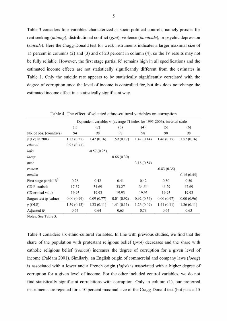
Table 4. The effect of selected ethno-cultural variables on corruption

Dependent variable: κ (average TI index for 1995-2006), inverted scale (1) (2) (3) (4) (5) (6) No. of obs. (countries) 94 98 98 98 98 98 y (IV) in 2003 1.83 (0.25) 1.42 (0.16) 1.59 (0.17) 1.42 (0.14) 1.46 (0.15) 1.52 (0.16) ethnoel 0.93 (0.71) lofre -0.57 (0.25) loeng 0.66 (0.30) prot 3.18 (0.54) romcat -0.83 (0.35) muslim 0.15 (0.45) First stage partial R2 0.28 0.42 0.41 0.42 0.50 0.50 CD F-statistic 17.57 34.69 33.27 34.54 46.29 47.69 CD critical value 19.93 19.93 19.93 19.93 19.93 19.93 Sargan test (p-value) 0.00 (0.99) 0.09 (0.77) 0.01 (0.92) 0.92 (0.34) 0.00 (0.97) 0.00 (0.96) y (OLS) 1.39 (0.13) 1.33 (0.11) 1.41 (0.11) 1.26 (0.09) 1.41 (0.11) 1.36 (0.11) Adjusted R² 0.64 0.64 0.63 0.73 0.64 0.63 Notes: See Table 3.

Table 4 considers six ethno-cultural variables. In line with previous studies, we find that the

share of the population with protestant religious belief (prot) decreases and the share with

catholic religious belief (romcat) increases the degree of corruption for a given level of

income (Paldam 2001). Similarly, an English origin of commercial and company laws (loeng)

is associated with a lower and a French origin (lofre) is associated with a higher degree of

corruption for a given level of income. For the other included control variables, we do not

find statistically significant correlations with corruption. Only in column (1), our preferred

instruments are rejected for a 10 percent maximal size of the Cragg-Donald test (but pass a 15

6

percent maximal test size). Our estimates of the income effect on corruption again remain the

same as before, with all OLS-estimates within the 95 percent confidence interval of the IV

estimates. More generally, we find with only one (narrow) exception that an estimate of 1.4 is

within the 95 percent confidence interval of all income effects reported in Tables 2-4.

4. The Corruption Transition

We follow Simon Kuznets (1965) and many later researchers by arguing that current cross-

country levels of income provide the best information about cross-country differences in long-

run development. Our paper uses the cross-country levels of income to explain the long-run

causality from income to corruption. We handle the problem of reverse causality by a unique

set of prehistoric measures of biogeography, which pass statistical tests for weak instruments.

Our main results are:

The cross-country pattern of corruption can be fully explained by the cross-country

pattern of income. To the extent that there is short-run interaction between corruption and

income – as there may very well be – it is irrelevant for the long-run effect. The long-run

causality is entirely from income to corruption. Corruption vanishes as countries get rich, and

there is a transition from poverty to honesty.

7

References: Clark, G., 2007. A Farewell to Alms: A Brief Economic History of the World. Princeton U.P., Princeton.

Deininger, K., Squire, L., 1996. A new data set measuring income inequality. World Bank Economic Review 10,

565-91.

Diamond, J., 1997. Guns, Germs, and Steel: The Fates of Human Societies. Norton, New York.

Galor, O., 2005. From stagnation to growth: Unified growth theory. Ch 4, 171-293, in Aghion, P., Durlauf, S.,

eds., Handbook of Economic Growth, Vol. 1A, North-Holland.

Gundlach, E., Paldam, M., 2008. A farewell to critical junctures. Sorting out the long-run causality of income

and democracy. University of Aarhus, School of Economics and Management, Economics Working

Paper, 2008-4. http://www.econ.au.dk/afn/abstr08/04.htm.

Hall, R.E., Jones, C.I., 1999. Why do some countries produce so much more output per worker than others?

Quarterly Journal of Economics 114, 83-116.

Hibbs, D.A.Jr., Olsson, O., 2004. Geography, biogeography, and why some countries are rich and others are

poor. Proceedings of the National Academy of Sciences of the United States (PNAS) 101, 3715-40. Kuznets, S., 1965. Economic Growth and Structure (Essays 1954-64). Norton, New York.

La Porta, R., Lopez-de-Silane, F., Shleifer, A., Vishny, R., 1998. The quality of government. Journal of Law,

Economics, and Organization 15, 222-79.

Lambsdorff, J.G., 2007. The Institutional Economics of Corruption and Reform. Cambridge UP, Cambridge, UK

Maddison homepage: http://www.ggdc.net/maddison/.

Maddison, A., 2003. The World Economy: Historical Statistics. OECD, Paris. Updated versions available from

Maddison homepage.

Masters, W.A., McMillan, M.S., 2001. Climate and scale in economic growth. Journal of Economic Growth 6,

167-86.

McArthur, J.W., Sachs, J.D., 2001. Institutions and geography: A comment. NBER Working Paper, 8114.

Olsson, O., Hibbs D.A.Jr., 2005. Biogeography and long-run economic development. European Economic

Review 49, 909-38. Paldam, M., 2001. Corruption and religion. Adding to the economic model. Kyklos 54, 383-414.

Paldam, M., 2002. The big pattern of corruption. Economics, culture and the seesaw dynamics. European

Journal of Political Economy 18, 215-40.

Paldam, M., Gundlach, E., 2008. Two views on institutions and development: The Grand Transition vs the

Primacy of Institutions. Kyklos 61, 65-100.

Parker, P.M., 1997. National Cultures of the World. A Statistical Reference. Greenwood Press, Westport, CT.

Transparency International homepage: http://www.transparency.org/.

Treisman, D., 2000. The causes of corruption: A cross-national study. Journal of Public Economics 76, 399-457. United Nations Office on Drugs and Crime (UNODC), 2005. The Eighth Survey on Crime Trends and the

Operations of Criminal Justice Systems (2001 – 2002). Downloaded from: http://www.unodc.org/.

8

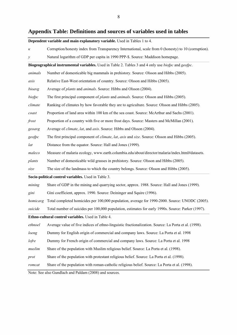
Appendix Table: Definitions and sources of variables used in tables

Dependent variable and main explanatory variable. Used in Tables 1 to 4.

κ Corruption/honesty index from Transparency International, scale from 0 (honesty) to 10 (corruption).

y Natural logarithm of GDP per capita in 1990 PPP-$. Source: Maddison homepage.

Biogeographical instrumental variables. Used in Table 2. Tables 3 and 4 only use biofpc and geofpc.

animals Number of domesticable big mammals in prehistory. Source: Olsson and Hibbs (2005).

axis Relative East-West orientation of country. Source: Olsson and Hibbs (2005).

bioavg Average of plants and animals. Source: Hibbs and Olsson (2004).

biofpc The first principal component of plants and animals. Source: Olsson and Hibbs (2005).

climate Ranking of climates by how favorable they are to agriculture. Source: Olsson and Hibbs (2005).

coast Proportion of land area within 100 km of the sea coast. Source: McArthur and Sachs (2001).

frost Proportion of a country with five or more frost days. Source: Masters and McMillan (2001).

geoavg Average of climate, lat, and axis. Source: Hibbs and Olsson (2004).

geofpc The first principal component of climate, lat, axis and size. Source: Olsson and Hibbs (2005).

lat Distance from the equator. Source: Hall and Jones (1999).

maleco Measure of malaria ecology, www.earth.columbia.edu/about/director/malaria/index.html#datasets.

plants Number of domesticable wild grasses in prehistory. Source: Olsson and Hibbs (2005).

size The size of the landmass to which the country belongs. Source: Olsson and Hibbs (2005).

Socio-political control variables. Used in Table 3.

mining Share of GDP in the mining and quarrying sector, approx. 1988. Source: Hall and Jones (1999).

gini Gini coefficient, approx. 1990. Source: Deininger and Squire (1996).

homicavg Total completed homicides per 100,000 population, average for 1990-2000. Source: UNODC (2005).

suicide Total number of suicides per 100,000 population, estimates for early 1990s. Source: Parker (1997).

Ethno-cultural control variables. Used in Table 4.

ethnoel Average value of five indices of ethno-linguistic fractionalization. Source: La Porta et al. (1998).

loeng Dummy for English origin of commercial and company laws. Source: La Porta et al. 1998

lofre Dummy for French origin of commercial and company laws. Source: La Porta et al. 1998

muslim Share of the population with Muslim religious belief. Source: La Porta et al. (1998).

prot Share of the population with protestant religious belief. Source: La Porta et al. (1998).

romcat Share of the population with roman-catholic religious belief. Source: La Porta et al. (1998).

Note: See also Gundlach and Paldam (2008) and sources.