The Transfer Efficiency Assessment of Individual Income · PDF file · 2007-03-01The Transfer Efficiency Assessment of Individual Income-Based Whole Farm Support Programs ... o n

The Transfer Efficiency Assessment of Individual Income-Based Whole Farm Support Programs

Technical Paper 5-95

Prepared by

Calum TurveyKarl Meilke

Alfons WeersinkKevin Chen

Rakhal Sarker

25 September 1997

Farm Management Solutions Inc. and The Department of Agricultural Economicsand Business, The University of Guelph

i

EXECUTIVE SUMMARY

Government intervention in agriculture is common place in Canada. During the lastthree decades farm support programs as well as support levels have increasedsubstantially. Because of growing fiscal deficits and public debts all government programsincluding those for agriculture are currently under review. Transfer efficiency of all farmprograms are being investigated and more efficient and trade friendly farm supportprograms are being sought. In light of the recent GATT Agreement, the current directionof Canadian agricultural policy is towards whole farm income stabilization and away fromtraditional commodity specific price and income support programs. New tools andconcepts are required to evaluate such whole farm based programs. The major objectiveof this study is to develop a framework capable of evaluating whole farm based programs.In addition to the theoretical framework, a prototype programming model is developed toexamine quantitatively the effects of various support programs on farm level productiondecisions. The report consists of five major sections.

Section two of the report reviews the classical economic arguments for governmentintervention in the market place including highly inelastic supply and demand,technological change, low farm incomes, incomplete contingency markets etc. To counterthese problems governments have undertaken actions to distribute income from one partof the economy (consumers and tax payers) to another (farmers). The measurement ofefficiency depends on what exactly is to be transferred and who is the intendedbeneficiary. Transfer efficiency is a measure of benefit distributions to the agri-foodsector. Payments targeted to farmers may involve seepage to input suppliers, processorsand consumers. Who gains, who loses and the degree of seepage depends very muchon the relationship between domestic and international markets. For example, most of thebenefits of transfer in a closed economy or in an economy with substantial market poweraccrues to consumers. However, in an export economy which is a price taker in the worldmarket, much of the benefit accrues to producers, suppliers of inputs and processors.

The first part of section three provides an overview of the existing support programsfor Canadian agriculture. It provides a brief historical perspective on the original intent ofthe current farm programs and how these programs evolved through time. The basicfeatures of each program are described and their possible future directions are discussed.While the future directions of traditional commodity based price and income supportprograms like GRIP, NTSP etc., are uncertain, the future of whole farm based supportprograms like NISA or VAISA looks quite promising at the present time.

The second part of section three provides alternative definitions and interpretationsof decoupled farm programs. The academic definition of decoupled programs differ fromtheir institutional definition. While most economists consider production neutrality as an

ii

important criteria for decoupledness, the GATT definition of the term emphasizes on thedegree of trade-distortion. So, a program may not be production neutral but it can still betermed decoupled under the GATT definition.

Based on the degree of trade distortions, all farm programs can be classified intosix major groups. Level 1 being the least trade-distorting and level 6 being the most.Level 1 refers to universal programs available to everyone; Level 2 constrains universalprograms available only to producers; Level 3 provides payments to producers and someproduction of agricultural goods is required; Level 4 payments are related to the level ofoutput but with limits; Level 5 provides open-ended direct payments related to the level ofoutput/input use; and Level 6 provides administered prices applicable to all output withborder controls and distorted consumption. Level 2-3 distortions would result from publicresearch and administration such as inspection, infrastructure, and domestic food aid;supply management would be a level 4 distortion; GRIP and NTSP would be a level 5distortion. It is unclear how NISA or VAISA would be considered since the GATT doesprovide criteria under which these programs would be `deemed' decoupled, including astipulation that payment can't be triggered for losses above 70% of long-run averages. Itis shown in section four that the NISA or NISA type programs would be risk as well asproduction neutral.

Section four of the report develops a general framework for analyzing the farm firmand examines the impacts of price stabilization/insurance and crop insurance, both ofwhich can be viewed as Level 5 distortions, on farm level production decisions. It takesa different view of the problem and in doing so, provides a rationale for criticizing the wayin which farm program distortions are defined and measured.

The premise here is that farmers are risk averse, and will, in the absence of farmpolicy, produce at a level of output below the optimum. With agricultural insurance tworesponses are recognized: First, the initial response by farmers is to increase output inresponse to decreased business risk (the risk adjustment effect); and second, asubsequent response to the degree by which premiums are subsidized in relationship tothe expected benefits of the program. It can be argued that the risk reduction effect is anatural response to the provision of contingent markets. The only reason governments getinvolved in such programs is that contingent markets are incomplete, and this has alreadybeen cited as a reason for intervention. If contingent markets were complete then farmerscould pay a premium to private insurers and speculators at least equal to the expectedbenefits. If such contingent markets were operated by the private sector they could not bedeemed trade-distorting, even though adoption of contingent instruments would, throughrisk sharing, lead to increased output.

In contrast, subsidizing premiums, whether privately or publicly, results in a furtherexpansion of output. It is this incremental increase in output which should be targeted bytrade agreements.

iii

Unfortunately this is not the way things work! Producer subsidy equivalents use anex post measure of subsidy which is based on total payments after risk realizations havebeen observed, and trade-distortion is measured relative to the total output effect, ratherthan the incremental effect to subsidization alone. Although it is possible that evencommodity specific policies can be deemed decoupled by the 5% de minimus standard.

In terms of transfer efficiency, benefits to producers, consumers and supplies ofinputs depend on the degree of risk aversion within the agricultural sector, the relativeelasticities of supply and demand, the existence of import and export markets and others.For example, programs used for commodities in which domestic production exertssubstantial market power, or programs which influence production of commodities forwhich there is international market power, will not result in a great amount of transfer goingto farmers, but rather to consumers, suppliers of inputs, and consumers in importingcountries. In contrast, if domestic producers are price takers whose actions have littleeffect on market prices, then most of the transfers will accrue to them and the suppliers ofinputs, with little benefit accruing to consumers. These transfers are impacted by relativelyinelastic supply curves which become more elastic or shift outwards, and relativelyinelastic input demand curves becoming more elastic.

The production and trade neutrality of commodity specific programs arequestionable. One should exercise caution, however, in making broad statements inregards to whether all policies fall into the GATT 'amber' category. There are tworesponses to stabilization. The first is through risk reduction. Farmers' response to riskreduction is a natural one and should not be considered an 'amber' response if premiumsare actuarially fair. For example, farmers will behave in a similar fashion to selection ofoptions on futures contracts as a risk management tool. The problem in regards to GATTand other trade agreements is in the subsidies associated with these policies rather thanthe policies themselves. Farmers' response to subsidies is an income effect whichexacerbates any output response from risk reduction. Therefore, any challenge to theseprograms by Canada's trading partners should be targeted only to the incrementalresponse to the income effect, not the risk reduction effect.

Since the gains from incremental risk taking are high relative to the possibleincrease in NISA contributions it is unlikely that NISA will encourage risk taking activities.On the contrary, as NISA savings become economically more important, farmers will havethe incentive to reduce revenue risks and they may achieve this through diversification intolower risk crops.

The results from the prototype model illustrate how agricultural policies affect farmlevel production decisions. The results indicate that none of the currently availablecommodity specific programs is decoupled. However, just because a program is notdecoupled does not necessarily mean that there will be an increased output response.Given limited resources, farmers will substitute the most favourable crops, increasing

iv

supply in some markets, but decreasing supply in others. The efficiency of agriculturalpolicies depends on the interrelationships among risky variables. In the above example,each crop was offered the same policy options, but still there were changes. Anotherissue relevant to the measurement of transfer efficiency is that not all policies are designedequiproportionately. Policy design can have a significant impact on the distribution ofresources within the farm, so that the true source of observed changes at the aggregatelevel cannot easily be distinguished. It is possible to examine these impacts at the farmlevel using simple optimization models such as the one presented here.

v

TABLE OF CONTENTS

1. INTRODUCTION . . . . . . . . . . . . . . . . . . . . . . . . . . . . . . . . . . . . . . . . . . . . . . . . . . 11.1. Background: . . . . . . . . . . . . . . . . . . . . . . . . . . . . . . . . . . . . . . . . . . . . . . . 11.2. Objectives and Organization of the Report: . . . . . . . . . . . . . . . . . . . . . . . 1

2. THE ECONOMICS OF TRANSFER EFFICIENCY . . . . . . . . . . . . . . . . . . . . . . . . . 2

3. SAFETY NET PROGRAMS VS. DECOUPLED FARM PROGRAMS . . . . . . . . . . 53.1. An Overview of Canadian Safety Net Programs for Agriculture: . . . . . . . 5

3.1.1. The Western Grain Transportation Act (WGTA): . . . . . . . . . . . . 63.1.2. The Future directions of the WGTA . . . . . . . . . . . . . . . . . . . . . . 83.1.3. Feed Freight Assistance Program (FFA): . . . . . . . . . . . . . . . . . . 93.1.4. The National Tripartite Stabilization Program (NTSP): . . . . . . . . 103.1.5. The Future of the National Tripartite Stabilization Programs in

Canada . . . . . . . . . . . . . . . . . . . . . . . . . . . . . . . . . . . . . . . . . . . . 113.1.6. The Gross Revenue Insurance Plan (GRIP): . . . . . . . . . . . . . . . 123.1.7. How Does GRIP Work? An Ontario Example . . . . . . . . . . . . . . 133.1.8. The Future of GRIP . . . . . . . . . . . . . . . . . . . . . . . . . . . . . . . . . . . 133.1.9. The Net Income Stabilization Account (NISA): . . . . . . . . . . . . . . 143.1.10. Value-Added Income Stabilization Accounts (VAISA): . . . . . . . 153.1.11. A Negative Income Tax (NIT): . . . . . . . . . . . . . . . . . . . . . . . . . . 16

3.2. Possible Future Directions of the Safety Net Programs for Agriculture . . 173.3. Decoupled Farm Programs: . . . . . . . . . . . . . . . . . . . . . . . . . . . . . . . . . . . 19

3.3.1. De Minimis Standard . . . . . . . . . . . . . . . . . . . . . . . . . . . . . . . . . . 223.3.2. Support for General Services . . . . . . . . . . . . . . . . . . . . . . . . . . . 223.3.3. Direct Payments Involving Supply Management . . . . . . . . . . . . . 233.3.4. Direct Payments to Producers Not Involving Supply

Management . . . . . . . . . . . . . . . . . . . . . . . . . . . . . . . . . . . . . . . . 23

4. A GENERAL APPROACH TO MEASURING THE TRANSFER EFFICIENCY OFGOVERNMENT SUPPORT PROGRAMS . . . . . . . . . . . . . . . . . . . . . . . . . . . . 254.1. The Firm's Response to Uncertainty: . . . . . . . . . . . . . . . . . . . . . . . . . . . . 264.2. Output and Price Uncertainty . . . . . . . . . . . . . . . . . . . . . . . . . . . . . . . . . . 264.3. The Effect of Price Insurance and Stabilization: . . . . . . . . . . . . . . . . . . . . 264.4. Market Impacts of Stabilization and Agricultural Insurance Policies: . . . . 314.5. The Transfer Efficiency of Crop Insurance: . . . . . . . . . . . . . . . . . . . . . . . 344.6. The Market Effects of Crop Insurance: . . . . . . . . . . . . . . . . . . . . . . . . . . . 374.7. Transfer Efficiency of Agricultural Insurance Policies: . . . . . . . . . . . . . . . 374.8. The Impact of Stabilization Programs on Input Demand and Input

Markets: . . . . . . . . . . . . . . . . . . . . . . . . . . . . . . . . . . . . . . . . . . . . . . . . 42

vi

4.9. NISA and Whole Farm Programs: . . . . . . . . . . . . . . . . . . . . . . . . . . . . . . 424.10. A Simplified Approach to the Analysis of NISA and NISA Type

Programs . . . . . . . . . . . . . . . . . . . . . . . . . . . . . . . . . . . . . . . . . . . . . . . . 434.10.1. An Analytical Approach to Analyzing NISA . . . . . . . . . . . . . . . . 44

4.11. Summary and Conclusions: . . . . . . . . . . . . . . . . . . . . . . . . . . . . . . . . . . 47

5. FRAMEWORK FOR INVESTIGATING TRANSFER EFFICIENCY . . . . . . . . . . . . 495.1. Incorporating the Stabilization Model Framework into the Deloitte and

Touche Framework . . . . . . . . . . . . . . . . . . . . . . . . . . . . . . . . . . . . . . . . 495.2. Transportation and Ad Hoc Subsidies . . . . . . . . . . . . . . . . . . . . . . . . . . . 505.3. Stabilization Programs . . . . . . . . . . . . . . . . . . . . . . . . . . . . . . . . . . . . . . . 515.4. Incorporating NISA into the Deloitte and Touche Framework . . . . . . . . . . 52

6.0 FARM LEVEL MODELLING OF COMMODITY SPECIFIC PROGRAMS . . . . . . 546.1. Risk Aversion . . . . . . . . . . . . . . . . . . . . . . . . . . . . . . . . . . . . . . . . . . . . . . 546.2. The B.E.A.R.Plus Farm Planning Program: A General Description . . . . 55

6.2.1 The Budget Module . . . . . . . . . . . . . . . . . . . . . . . . . . . . . . . . . . . 556.2.2 The Financial Statements Module . . . . . . . . . . . . . . . . . . . . . . . . 55

6.3. B.E.A.R.Plus and Whole Farm Optimization . . . . . . . . . . . . . . . . . . . . . . 556.4. The Prototype Farm Planning Model . . . . . . . . . . . . . . . . . . . . . . . . . . . . 566.5. Potential Market Response to Agricultural Insurance: . . . . . . . . . . . . . . . 646.6. Summary and Conclusion . . . . . . . . . . . . . . . . . . . . . . . . . . . . . . . . . . . . . 64

REFERENCES . . . . . . . . . . . . . . . . . . . . . . . . . . . . . . . . . . . . . . . . . . . . . . . . . . . . . . 66

Appendix A: Risk Aversion and Production . . . . . . . . . . . . . . . . . . . . . . . . . . . . . . 68

Appendix B: Truncated Risk and the Pricing of Insurance . . . . . . . . . . . . . . . . . . 69

Appendix C: Crop Insurance . . . . . . . . . . . . . . . . . . . . . . . . . . . . . . . . . . . . . . . . . . 71

Appendix D: Impact of Stabilization on Input Demand and Input Markets . . . . . 73

1

1. INTRODUCTION

1.1 Background:

Governments of western democracies have been transferring considerable amountof public funds to their respective agricultural sectors through various price and incomesupport programs since the Second World War. The number of such farm supportprograms as well as the levels of protection afforded have grown substantially throughtime. The growing fiscal deficits and public debt problems in these countries in the 1990sgenerated public pressure for rational evaluation of all government programs.Consequently, the programs for agriculture are also being placed under the microscope.Two major issues are being considered: (1) how efficient the existing farm programs arein transferring income to agriculture? and, (2) how can the farm programs be changed orrepackaged to make them more efficient?

Agriculture Canada contracted Deloitte & Touche Management Consultants toinvestigate the effects of agricultural programs on the agri-food sector. The Deloitte &Touche report, How Governments Affect Agriculture, provides a framework for assessingtransfer efficiency of various agricultural programs. The report examines how the benefitsof government farm programs are shared among farmers, input suppliers, processors,consumers and government agencies. The study, however, focuses on the aggregatelevel with little emphasis on what happens at the farm level. Moreover, in light of therecent GATT Agreements there is a greater demand for developing domestic farm policieswhich are trade friendly.

1.2 Objectives and Organization of the Report:

One of the major objectives of this study is to analyze the rationale for, and theeconomic effects of trade friendly policies that reduce farmers production and consumptionrisks. The current direction of Canadian agricultural policy is away from commodityspecific price and income support towards whole farm income stabilization. The analysesof this type of program requires tools and concepts not previously applied to the evaluationof government programs. This study is an attempt to fill part of this knowledge gap. Thesecond major objective is to develop a prototype empirical model to examine how variousgovernment policies affect farm level production decisions.

Section two defines transfer efficiency and provides a brief review of the literatureon transfer efficiency. Section three provides an overview of current safety net programsfor Canadian agriculture. Section three also provides alternative definitions of decoupledfarm programs with particular emphasis on the GATT (1994) criteria for decoupledprograms. Section four develops a general framework for measuring the transfer efficiencyof various government support programs. The analysis focus on farm level decision

2

making rather than on the farm sector as a whole. Section five outlines an empiricalmethodology and develops a prototype model. Using the prototype model, this sectionalso illustrates how various agricultural programs affect farm level production decisions.

3

2. THE ECONOMICS OF TRANSFER EFFICIENCY

Transfer efficiency is broadly defined as a measure of benefit distributions withinthe agri-food sector and effectiveness in farm income transfer due to governmentagricultural support programs and initiatives. In examining the efficiency of governmentprograms and how such efficiency has been modeled, it is instructive to initially examinewhy governments intervene in the agricultural sector. The dominant view has been thatagricultural policy is necessary to solve social problems related to market failures. A morerecent alternative view is that government intervention is the result of rent seekingactivities by producers.

The social problem that has tended to justify government aid to the agriculturalsector is the tendency for low commodity prices to cause sudden drops in farm income andthe secular decline in the number of farms. This "farm problem" has often been explainedin terms of simple supply and demand concepts. The basic features of agriculturecharacterized by this model are the highly inelastic demand, the slow growth of totaldemand, rapid technological change which increases supply over time, and the tendencyof resources to become fixed within the industry (Rausser and Hochman, 1979). Sincesupply has historically increased faster than demand, real commodity prices have fallen.Asset fixity with limited labour mobility means that the price decline is translated throughto lower farm income and return on investments (Gardner, 1987b).

The farm problem scenario would predict chronic declines in land prices and farmwage rates, given the declining commodity prices over the last several decades. However,this has not occurred and farmers may be described as relatively wealthy. Thus, therationale for public intervention in agriculture is now focused on public goods argumentsinvolving the correction of market failures (Gardner, 1992). Several types of failures havebeen identified by Stiglitz (1987) to justify government support as a second-best policy.One failure is the incompleteness of insurance and credit markets to stabilize income forfarmers who are subject to large and unpredictable market risks. A second is the level andvariability of farm income which has been viewed as unacceptable by society. Anotherpossible failure is imperfect competition in the markets faced by producers (McCalla andCarter, 1976). A fourth market failure that makes intervention attractive involves the publicgood aspects of information and the generation of new technology (Gardner, 1992).Another market failure is the existence of environmental externalities which may justifyinterventions such as government subsidization of soil conservation practices.Understanding the primary reasons for agricultural policy are necessary in order toevaluate their effectiveness.

Each possible form of government intervention will have positive and negativeeffects on at least part of the public. In order to evaluate the gains and losses from thealternate policy options, an objective method is required. Welfare economics has provided

4

for the base for that method of measuring and weighting the net benefits (or losses) tomarket participants. The following review briefly summarizes how welfare economics hasbeen used by agricultural economists to examine the transfer efficiency of governmentpolicy. The review highlights how the definition of transfer efficiency has been broadenedover time.

The first studies estimating the benefit and costs of farm programs were by Wallace(1962) and Nerlove (1958). The redistribution of producers' and consumers' surplus undervarious policy instruments were approximated from data on the price wedge created by thepolicy and elasticities of supply and demand. The approach introduced by Wallace andNerlove has been followed by most subsequent studies. The refinements to the basicsupply and demand model are outlined below.

Efficient redistribution of income to support agriculture would increase producersurplus by a dollar, for every dollar that consumer surplus fell. In a single commoditymarket, as examined by Nerlove and Wallace, Gardner shows how a surplustransformation curve can be obtained by solving for the producer surplus as a function ofconsumer surplus. The deadweight loss can then be depicted as the distance betweenany point on this curve and the efficient redistribution line. The optimal intervention canbe found through the use of a social welfare function which aggregates consumers' andproducers' surplus.

In reality, commodity markets are not isolated from one another. In addition, theinconsistencies resulting from the simple formulation of the farm problem as outlinedabove, has led to more detail in specifying supply-demand for agricultural factors ofproduction and their relationship to commodity markets. However, the efficiency ofmultimarket commodity programs can not be found by simply summing the net gains ineach market individually and in isolation from other markets. For example, the effects ofa price rise in one commodity depends upon its substitutability with other products. Theefficiency of programs in multimarkets consequently not only depends on the supply anddemand elasticities of a single good, but also on the elasticity of substitution betweeninputs; the supply elasticity of these inputs, who owns the inputs, and the cross elasticitiesof demand for other products. The beneficiaries under this model have been expandedfrom only aggregate producers and consumers under the supply and demand model of asingle market to include producers and consumers of various outputs and inputs. Thismodel has been used by Deloitte and Touche in their 1992 analysis of net benefits ofgovernment programs and in their 1993 report on how governments affect agriculture.Maier has extended (1994) this analysis to examine the effects at different stages in themarketing chain and for the impacts of imperfect competition.

Gardner (1987b) presents various refinements to the multimarket supply anddemand model now used as the standard to examine the transfer efficiency of governmentpolicies. One of the extensions is to account for rational expectations where the producer

5

decides how much to produce based on the best information available about future marketconditions at the time that production decisions are made. Related to the issue ofincomplete information is the inherent uncertainty in agriculture which, as discussedearlier, can be used to justify government action. Instability associated with sharp shortterm price fluctuations, random production due to natural events, unpredictedmacroeconomic policies etc. impose losses on people which may be moderated bygovernmental intervention. Assuming farmers are risk averse there are social benefits ofrisk reduction since farmers will produce more when revenues fluctuate less. Thesubsequent increase in supply will then lower consumer prices. Just, Hueth and Schmitz(1982) show how such producer gains can be measured and conclude that the moreinelastic the demand function, the more likely that risk averse producers will gain fromstabilization. However, Gardner (1987a) concludes that policy analyses have not beenable to incorporate risk considerations quantitatively in any convincing way. Instead, hesuggests consideration of risk may be more fruitfully introduced in terms of the supply anddemand for price insurance rather than by modifying commodity supply and demandfunctions.

The closed economy models outlined above can be substantially altered byinternational trade considerations. For example, an increase in the producer support levelmay not result in the expected decrease in consumer prices if the region is a price takerin the world market. The text by McCalla and Josling (1985) summarizes the basiceconomics of alternative policy instruments for importing and exporting countries. Themodel has been applied by de Gorter and Meilke (1989) in their evaluation of policiesbeing considered by the EC in modifying the Common Agricultural Policy.

A final element to be considered in the assessment of the efficiency of governmentprograms is the excess burden of taxation imposed on the public through the cost of theseprograms. Substitution effects created by taxes alter economic decisions and create a lossin welfare in addition to the tax revenues collected. Given the possibility of distortionarycosts from general income (sales) taxes, it is important to examine whether payments tofarmers financed from the collection of these taxes is more or less efficient than consumertransfers to farmers via commodity market intervention (Deloitte & Touche, 1993). Alstonand Hurd (1990) propose that taxes be put on specific agricultural commodities until themarginal deadweight cost of distorting consumption in that commodity equals the marginaldeadweight costs of the existing income tax. However, Ballard and Fullerton (1992) arguethat the marginal excess burden of taxation is close to zero. Deloitte & Touche assumethis value for general expenditure programs but not for programs based on raising marketprices.

6

3. SAFETY NET PROGRAMS VS. DECOUPLED FARM PROGRAMS

3.1 An Overview of Canadian Safety Net Programs for Agriculture:

Safety net programs have been an integral part of Canadian agriculture during thepost-war period. During difficult times, agricultural producers across Canada havebenefited from various support programs under the: Agricultural Stabilization Act (ASA),Western Grain Stabilization Act (WGSA), Crop Insurance Act (CIA), Western GrainTransportation Act (WGTA), Feed Freight Assistance (FFA), Tripartite Stabilization etc.Some of these programs have been modified during the 1970's and in the early 1980's tomake them more efficient under the changing economic environment.

Although the modifications served the interests of farm producers during the late1970's and early 1980's, developments outside the Canadian economy made some of thesafety net programs less effective during the late 1980's. This is particularly true for thegrains and oilseeds sectors. The emergence of the European Union as a surplus producerof grains and oilseeds intensified the competition for export markets and led to competitivesubsidization between the United States and the EU. Small exporters like Canada,Australia and Argentina were caught in the middle. The price of major grains, especiallywheat in the international market, fell below $90/t. Even efficient Canadian producerscould not cover their costs of production at this price. The safety net programs such asthe WGSA and the ASA were judged not to provide enough financial support to grainproducers under these circumstances. The federal and provincial governments deviseda Special Assistance Program for grain and oilseed producers (called the Special CanadaGrains Program). Under this special assistance program several billion dollars weretransferred to prairie grain and oilseed producers during the late 1980's. Despitenegotiations between the U.S. and the EU, and the launch of the GATT negotiations, theinternational agricultural trade situation remained largely unchanged. The specialassistance programs also generated an equity debate between grain and oilseedproducers in eastern and western Canada. Moreover, some of the Canadian safety netprograms were coming under increasing criticism during the Uruguay Round of GATTnegotiations.

Under these circumstances, the federal Minister of Agriculture initiated the NationalAgri-Food Policy Review in November 1989. The review was based on four basicprinciples: market responsiveness, self reliance, regional sensitivity and environmentalsustainability. As a result of this review a safety net committee made up of farmers, andfederal and provincial representatives was formed to provide advice on the longer termneeds and sustainability of the agricultural sector. Based on the recommendations of theAgri-Food Policy Review, the federal government established the Grain and Oilseed SafetyNet Task Force in January 1990. The responsibility of the task force was to develop a newnational safety net program for the grain sector which could deal with low farm gaterevenues. The task force recommended in January 1991, the establishment of the Gross

7

Revenue Insurance Plan (GRIP) and the Net Income Stabilization Account (NISA) as newsafety net programs for agriculture. In March 1991, the Minister of Agriculture tabled thesafety net legislation in the form of the Farm Income Protection Act (FIPA) [Bill C-98]. Thisbill consolidated all existing safety net programs as well as the newly developed programs,GRIP and NISA, under one Act. FIPA also repealed ASA, WGSA and CIA. Through theintroduction of GRIP and NISA, the Farm Income Protection Act has dramatically alteredthe nature of agricultural stabilization in Canada.

The objective of this section is to provide an overview of the existing supportprograms for Canadian agriculture. The programs were designed to address the price,income and welfare concerns of various commodity groups from time to time. Although theoriginal intent of most farm program has changed through time, to have a betterunderstanding of the policies and programs, an attempt is made here to briefly documentthe original intent of each of the existing programs. The basic features of each of theprograms are described and the possible future directions of the programs are discussed.Finally, an attempt is made to define decoupled farm programs and rate existing farmprograms in Canada on the scale of acceptability under the recently concluded GATTAgreements.

3.1.1. The Western Grain Transportation Act (WGTA):

During the late 19th century and early 20th century the federal government usedimmigration policies and grain transportation subsidies as key instruments for regionaldevelopment in western Canada. As an important component of the regional developmentstrategy, the federal government signed an agreement with the Canadian Pacific Railway(CPR) in 1887, popularly known as the Crow's Nest Pass Agreement. Under thisagreement, the federal government provided a subsidy for the construction of a 300 milerail line from Lethbridge, Alberta to Nelson, British Columbia and the CPR, in return,agreed to a rate ceiling for moving grain and grain products eastward on its lines. TheCPR also agreed to rate ceilings for moving a variety of settlers' effects to the west. Therate ceilings for settlers' effects were discontinued in 1925 and the rates were fixed instatue for grains. A number of amendments were made to the Agreement over the yearsto make grain by-products and oilseeds eligible for the special rates. From time-to-time,the federal government intervened to maintain freight rate differentials between raw andprocessed products from prairie agriculture. The primary objectives of this agreementwere to stimulate agricultural production, particularly grains and oilseeds in the prairieregion, and to reduce the financial risks to the railway companies associated with theconstruction of railroads across the prairie region, which was sparsely populated andunderdeveloped at that time. The secondary objective was to keep the U.S. expansionforces at bay from western Canada.

The railway subsidy worked well for agricultural growth in western Canada. Grain

8

transportation subsidies along with the production incentives implicit in various price andincome stabilization programs, introduced since the Second World War, resulted in a hugeexpansion of agricultural production in the prairie region. New export opportunities abroadand technological progress in agriculture sustained the momentum for expansionaryagriculture. In the early 1960's, while the cost of labour and other inputs increased dueto inflation, the statutory grain-rail rates remained fixed at the 1925 levels. As a result,Canadian railways were experiencing growing revenue losses on grain shipments. In1961, the MacPherson Royal Commission reported that the railways were losing moneyin grain transportation. Consistently large revenue shortfalls on grain shipments startingin 1960, and the lack of public support for freight adjustments to reflect changedcircumstances led to the deterioration of the grain transportation system. During the mid1970's when the export demand for Canadian grains increased significantly, the railwaycapacity to handle the increased grain shipments to the export ports became limiting. Thishelped to focus public attention on the fixed grain transportation rates.

In 1975, the Minister of Transport established the Snavely Commission toinvestigate the costs and revenues associated with transporting statutory grains by therailways, and the Grain Handling and Transport Commission, headed by Justice E. Hallto evaluate the needs for prairie rail branch lines. The Snavely Commission reported thatthe cost of transporting grain was 2.6 times higher than the statutory rate being paid by theproducers while the Hall Commission recommended streamlining some prairie rail branchlines. In light of the findings of these commissions, a number of ad hoc measures weretaken to fix the deteriorating grain transportation system and to expand its capacity;boxcars were repaired, hopper cars were purchased, ports were improved. Despite thesemeasures, the grain transportation system continued to deteriorate. Under thesecircumstances, on Feb. 8, 1982 the federal government initiated a consultative process ledby Dr. J.C. Gilson. A number of major policy and financial parameters recommended byprevious commissions on grain transportation were used to guide the consultations. A setof basic principles to reform the grain handling and transportation system in Canadaemerged from the Gilson consultation process. Based on the recommendations of thisconsultation process, the federal government passed the Western Grain TransportationAct (WGTA, Bill C-155) in 1983 (Tyrchniewicz 1984).

The key provisions of the WGTA are as follows:

1. Freight Rates: Under this Act freight rates are set each crop year for movinggrain and grain products and oilseeds to various export destinations. The rates are basedon forecast grain volumes, provided by the Grain Transportation Agency (GTA), and theestimated costs to the railways of moving grains to different ports, calculated by theNational Transportation Agency (NTA). The freight rate structure is distance-based andis shared by the producers and the government. In 1993/94, for example, the producersand government shares of the freight rate were 42.8% and 57.2% respectively. For ahauling distance of 976-1000 miles the rate was $32.07/tonne; the producer paid

9

$13,73/tonne and the rest was paid by the government. In the future, the producers' shareof the freight rate is expected to rise gradually.

2. Crow Benefit: The Crow Benefit is the federal government's revenue shortfallcommitment to the railways under the WGTA. The Act provides for the payment of the1981-82 railway revenue shortfall of $659 million on an annual basis by the federalgovernment to the railways. This payment has been made entirely to the railways up tonow. According to the Federal Budget of 1995, this Crow Benefit subsidy will beterminated on July 31, 1995.

3. Future cost sharing: The producers would pay a maximum of 3% per year ofthe future cost increases until 1985-86; any additional cost increases would be borne bythe federal government. Beyond the 1985-86 season, the producers share would rise to6% per year. This provision is no longer relevant. The Crow subsidy will be eliminatedon July 31, 1995. The grain shippers will have to pay the full grain shipment costs by railstarting from August 1, 1995. However, the maximum legislated grain freight rates will beretained until 2000.

4. Volume Limitation: The Act provides for a volume cap of 31.5 million tonnesof grain. If shipments are higher than 31.5 million tonnes, the additional volume is chargedthe full cost of transport. This will be less binding after August 1, 1995 and irrelevant after1999 when the grain freight rates are expected to be deregulated.

5. Shipper Share Limitation: Under this legislation, the producers share of thefreight rate would not be allowed to exceed a fixed percentage of the weighted averageprice of the six major grains. The share was increased from 4% in 1984 to 10% in 1988.This provision has not been activated so far.

6. Eligible Commodities: The list of eligible products was expanded to includecanola seed, oil and meal, linseed oil and meal, sunflower seed and oil, corn, mustardseed, canary seed, triticale, dehydrated alfalfa, and peas, beans, lentil, and theirderivatives.

7. Grain Transportation Agency (GTA): The Act establishes the GrainTransportation Agency (GTA) and the Senior Grain Transportation Committee, andoutlines their responsibilities. In particular, the GTA is responsible for promoting systemefficiency, monitoring railway performance and investment, and rail car allocation. Underthe Act, the GTA may "hold back" some portion of the annual subsidy to the railways if therailways do not meet performance and investment standards.

8. Costing Review: The Act requires the National Transportation Agency (NTA)to review the railways costs of moving grain every four years. The Act also requires theMinister of Transportation to undertake a review of the operations of the major sections of

10

the Act on a regular basis.

3.1.2. The Future directions of the WGTA:

The domestic and international production and trade environments have changedsignificantly since the 1980s. The interests and issues which generated the need for theCrow's Nest Pass Agreement and the subsequent enactment of the Western GrainTransportation Act are not as relevant as they were in the past. The transport subsidiesare now considered as impediments to the diversification of prairie agriculture favouringthe production of high value crops and livestock products. The federal governmentsfinancial commitments are also expected to change in light of increasing fiscal constraints.Moreover, under the recent GATT Agreement, the WGTA subsidies are considered exportsubsidies. In the Federal Budget of 1995, the annual subsidy under the WGTA has beenterminated. Farmers shipping grains will have to pay the full grain shipment costs via railstarting from August 1, 1995. A one-time payment of $1.6 B will be made to prairie farmersas compensation for the loss of their crow benefits.

3.1.3. Feed Freight Assistance Program (FFA):

The Feed Freight Assistance program was originally conceived as a war timemeasure during the Second World War. In 1941, the Federal Department of Agricultureintroduced this program in an effort to increase livestock production required to meet thewar-time demand for meats. Under this program, the federal government paid a subsidyon the transportation of feed grains from the prairie provinces to eastern Canada andBritish Columbia. This program lowered the delivered cost of feed grains to livestockproducers both in Eastern Canada and British Columbia. Since there were effective pricecontrols over meats during the war, the FFA subsidy ensured a reasonable profit forlivestock producers across Canada. The objectives of the program were as follows:

1. To make available adequate supplies of feed to maintain livestock productionfor domestic and export requirements;

2. To keep the costs of livestock production down during a period of pricecontrol over livestock and livestock products; and,

3. To equalize prices paid by users of feed grains across Canada.

The program was so rich during the war time that it virtually eliminated the freightcost of moving feed grains from the prairie provinces to feed deficit areas (i.e., Ontario,Quebec, Maritime provinces and British Columbia). Although it was initiated as a war time

11

measure, it became a part of the post-war Canadian agricultural policy. During the post-war period, the continuation of the FFA was viewed as a way to preserve domestic marketsfor prairie grains. The original FFA program, however, has undergone a series of changesduring the last four decades in response to changes in market conditions.

The opening of the St. Lawrence Seaway in 1959 reduced the costs of transportinggrains to Ontario and Quebec and the FFA rates were adjusted to reflect this. In 1966, thefederal government enacted the "Livestock Feed Assistance Act" (LFAA) and establishedthe Canadian Livestock Feed Board (CLFB). The Board was given the responsibility ofensuring adequate supplies of feed grains to livestock producers in eastern Canada andin British Columbia at reasonably stable and fair prices. The Board was also responsiblefor making payments under the FFA program. In 1967, feed corn grown in Ontario andshipped to the Atlantic provinces became eligible for FFA payments. The FFA rates weremodified in a major way in 1976. The subsidies under the FFA were eliminated for Ontarioand western Quebec and the rates were reduced for the central Quebec. The rates fornorthern and eastern Quebec and for the Atlantic provinces remained unchanged. In1980, transportation of feed grains to the Yukon and Northwest Territories became eligiblefor the FFA payment. Finally, in 1984, all feed grains of Canadian origin (local as well asthose produced in other Canadian provinces), which passed through the commercialchannels to users in areas eligible for FFA payments, were made eligible for FFA. Alsothe rates were raised for the Maritime provinces so that the grain prices paid by theMaritime users remained at par with the prices paid by grain users in Montreal. Since1990, transportation costs beyond the lower St. Lawrence (up to $50/tonne) are eligiblefor the FFA subsidy. In 1990, the dairy and poultry sectors received about 67% of the FFAsubsidies and British Columbia was the largest beneficiary (about 30% of total paymentsunder the FFA).

The Federal Budget of 1995 has also eliminated the FFA subsidy. As of October1, 1995, the FFA will cease to exist. An adjustment fund has been created to help thefarmers benefiting from the FFA subsidies.

3.1.4. The National Tripartite Stabilization Program (NTSP):

The amendments to the ASA in 1975 represented a significant commitment on thepart of the federal government to stabilize farm income (not only farm prices) at a politicallyacceptable level. It expanded the commodity coverage, changed the base period from aten year to a five-year moving average, increased the guaranteed minimum support levelfrom 80% to 90% of the base period price, introduced cost indexing of the support pricesand introduced provisions for joint federal-provincial programs to provide support levelshigher than the minimum guaranteed prices in the ASA. While these amendments weresupported by most farm groups at that time, steadily increasing feed prices during the earlyand mid 70's made these programs rather unattractive for livestock producers. British

12

Columbia and Quebec introduced provincial income support programs for red meatproducers which were considerably richer than those provided under the ASA. The redmeat producers in other provinces put pressure on their respective provincial governmentsto implement similar programs.

A wide variety of provincial programs for the red meat sector emerged between themid-1970's and the mid-1980's. While these programs were voluntary and requiredproducers contributions, the richness of the programs varied considerably acrossprovinces raising serious concerns about the equity of support levels offered. The equitysituation deteriorated despite the threat from the federal government for a dollar-for-dollardeduction from its payment under the ASA to provinces which had richer provincialprograms. The proliferation of provincial commodity-based price and income supportprograms also generated a national economic and political problem.

Under these circumstances, the federal and provincial authorities initiateddiscussions on "tripartite stabilization" programs in the fall of 1977. In January 1985, theASA was amended to allow the formation of tripartite agreements. Tripartite Stabilizationprograms for red meats were effective on January 1, 1986 for Alberta, Saskatchewan,Manitoba and Ontario. Tripartite agreements were signed by other provinces for redmeats, at a later date. Similar tripartite stabilization agreements were also signed forbeans, apples, honey and sugar beets. Thus, the dissatisfaction of red meat producersand other commodity groups with the level of support payments under the 1975 ASA andthe subsequent proliferation of provincial support programs were largely responsible forthe establishment of tripartite stabilization programs in Canada. The tripartite stabilizationprograms are commodity specific and some aspects of the programs are designed to suitethe needs of specific commodity groups. There are, however, certain generic features ofthe program. Those are as follows:

1. Nature: All producers of a particular commodity receive the same level ofsupport per unit of production across Canada. All commodity plans established under thenational tripartite program receive a comparable level of support.

2. Program Costs: All costs of the program are shared equally by the federal andprovincial governments and participating producers. For some commodities(e.g., hogs,cattle and lambs), restrictions are in place for the maximum share of the program costs tobe borne by the federal and provincial governments.

3. Support Levels & Payouts: Under this program, support levels are determinedbased on a guaranteed margin approach. Stabilization payments are made to theproducers if the current year's margin falls below the minimum guaranteed margin.

4. Entry and Exit: In most cases, enrolment is voluntary up to the initial deadline.After the initial deadline, enrolments are subject to a phase-in rule. Under a phase-in rule,

13

a new participant will pay the full premiums for a certain period but will receive only partial(but gradually increasing [25% first quarter/year, 50% next, followed by 75% and finally100% of the payments]) share of any declared stabilization payments. Producers canwithdraw from the program by giving a notice three-years in advance. Producers whowithdraw cannot rejoin the program until two years after the withdrawal takes effect. Anyproducers who may want to rejoin the program are considered late entrants and aresubject to the phase-in rule. Thus, in most cases, entry and exit are rare.

3.1.5. The Future of the National Tripartite Stabilization Programs in Canada:

Like many other agricultural support programs currently available, the future of theNTSP is uncertain. Under the recently concluded GATT rules, stabilization payments areproduction and trade distorting and hence, countervailable by Canada's trading partners.It is, indeed, a challenge to devise agricultural stabilization programs which providepolitically acceptable levels of support to commodity producers and yet are consideredGATT green (i.e., decoupled under GATT rules). The NTSPs for cattle and hogs havealready expired as of December 31, 1994. These programs have not been renewed orreplaced with any other programs. Indications are that the remaining tripartite stabilizationprograms will also be discontinued. A number of discussions have been initiated toreplace the NTSPs with VAISA type programs. It remains to be seen how such VAISAprograms would be designed.

3.1.6. The Gross Revenue Insurance Plan (GRIP):

The Gross Revenue Insurance Plan is one of the two major safety net programsestablished under the FIPA of 1991. In fact, because of its remarkable departure fromprevious safety net programs for grains and oilseeds, GRIP has generated muchdiscussion and debate among farmers and policy makers across Canada. At the time ofits introduction, GRIP had been hailed in the policy making circle as a new generationsafety net program which would eliminate differences in financial support to grain andoilseed producers in eastern and western Canada. The last four years of operationindicate that GRIP has failed to offer harmonized supports to grain and oilseed producersacross Canada. Indeed, provincial top-loading continues through GRIP. Consequently,the GRIP in one province looks quite different than the GRIP in another province; both thestructure of the program and support levels vary considerably across provinces (Turveyand Chen 1994).

The primary objective of GRIP is to provide gross revenue protection to grain andoilseed producers. In the past, price protection was offered largely through the ASA andthe WGSA and limited yield protection was provided through crop insurance programs.The intent of providing price and yield protection through a single program was a clear

14

departure from past tradition. In principle, GRIP is a tripartite stabilization program thedirect costs of which are shared by the federal and provincial governments and farmers.The basic features of GRIP are as follows:

1. Nature: GRIP is a commodity-based voluntary insurance program in whichparticipating farmers pay premiums and receive indemnities if their market revenues fallbelow the target revenues in a particular year. GRIP consists of two basic components:crop insurance and market/gross revenue insurance. In some provinces, these twocomponents are integrated but they are offered separately in the majority of the provinces.

2. Administration: GRIP is administered provincially. The federal and provincialgovernments equally share the administrative costs of the program. The cost of insurancepremiums is shared by the federal and provincial governments and farmers. Farmers pay33%, the federal government pays 42% and the provincial government pays 25% of theinsurance premiums.

3. Commodity coverage: All grain and oilseed crops covered by crop insuranceare eligible for GRIP benefits. In addition, on-farm fed grain and grain crop silage are alsoeligible for this program.

4. Support levels: The support levels for each eligible crop under GRIP aredetermined by using target price and target yield levels. The target price for a crop isdetermined as the 15-year moving average provincial price for that crop adjusted forchanges in Farm Input Price Index. The target yields are the historic average yield figuresdefined by crop insurance. For those not in the crop insurance, average yields of the last7 to 15 years (depending on the province) are used as target yields. In most cases, 80-90% of the indexed moving average prices and 70-95% of the historic average yields areused as target figures to calculate indemnities for participating farmers.

5. Payouts: Payouts under GRIP are issued though the provincial crop or incomeinsurance agencies. Provinces can make up to three interim payments and one finalpayment. Interim payments, however, are limited to a maximum of 75% of the totalpayment for the year. Since the payout levels for GRIP are based on the differencebetween the target revenue and the market returns for a given year, program payouts canresult in a deficit. If a deficit is incurred, the federal and provincial governments advance65% and 35% of the deficit respectively.

6. Entry and Exit: While entry into the GRIP is perfectly voluntary, exiting theprogram is not. Producers are required to give an exit notice three-years in advance. Inaddition, a farmer is not allowed to re-enter the program for two years after opting out.However, producers exiting grain farming or leaving farming for good are not penalized.

15

3.1.7. How Does GRIP Work? An Ontario Example:

Ontario has adopted a GRIP formula which combines market revenue insurancewith crop insurance. The target price is based on 80% of the 15 year moving-averageOntario price and the target yield is 80% of the individual producer's long-run averageyield. Suppose the 15 year average price is $3.82/bu. and average yield is 120bu./acre.Also, suppose the farmer insured 90% of his historic yield through crop insurance (i.e., at108bu./acre). If, in a particular year, his yield drops to 60bu./acre and market price is only$2.50/bu., then he receives a payout through market revenue insurance worth (($3.18-$2.50)*(0.80*120)) or $65.28/acre. Crop insurance gives him another $120.00/acre. Hismarket revenue is $150.00/acre but his total (gross) revenue including the GRIP benefitis $335.28/acre.

3.1.8. The Future of GRIP:

The future of GRIP is not very promising. There are economic and political reasonsfor this grim forecast. The program did not deliver comparable financial benefits to farmersin eastern and western Canada. During the first two years of the program when the worldgrains markets were depressed, the 15-year indexed moving average price (whichincluded high real prices from the mid to late 1970's) were very attractive and farmersreceived substantial financial support through the program. However, the indexing formulahas no relationship to current market conditions and hence the policy is rooted in the past.The averaging procedure will also eventually reduce the GRIP benefits causing an exodusfrom the program when payments seem remote.

The actuarial soundness of the GRIP is still a big question. The program hasaccumulated almost a billion dollar deficit during its first four years. While actuarialsoundness is related to the entire life of the program and net payouts are expected duringinitial years, the voluntary nature of the program makes it difficult to predict the life spanover which the GRIP would be actuarially sound. Evidence suggests that the premiumscharged have little relationship to the underlying crop risks. Critics also argue that relativeto other farm programs GRIP has a higher potential for generating moral hazard andadverse selection problems in agriculture. These problems may also jeopardize the long-run viability of the GRIP as a safety net program. Experts have also voiced their concernsabout altered crop portfolio choices induced by GRIP. While these are all legitimateconcerns, it is too early to undertake any empirical assessment of these inadequacies.

There are indications that GRIP may suffer a premature death. Its survival needsparticipation from all provinces. Newfoundland did not implement GRIP, Saskatchewanpulled out of the program at the end of the 1994 crop year and Manitoba is likely to exit atthe end of 1995. Alberta has also given a notice of withdrawal. In view of its richness,adverse resource allocation effects at the farm level and its long-run financial viability, the

16

current federal government is planning to discontinue the program and replace it with awhole-farm based income insurance program.

3.1.9. The Net Income Stabilization Account (NISA):

The Farm Income Protection Act of 1991 introduced a second safety net programfor agriculture in addition to GRIP called the Net Income Stabilization Account (NISA).This program provides income stabilization through an individual account whichencourages farmers to set aside money in individual accounts in high income years for usein bad years. NISA is designed as a whole farm based program in which participatingfarmers must register all crops. Other distinguishing features of NISA are as follows:

1. Contribution: NISA is a voluntary program. Once enroled in NISA, a farmer canhave his or her own NISA account. He can contribute up to 2% of eligible net commoditysales (defined as gross farm receipts minus the cost of seed, livestock and feedpurchased) in the NISA account each year. This amount receives a matching contributionfrom the government. The maximum net sale qualifying matching government contributionis set at $250,000 per farm. The cost of the matching deposits are split equally betweenthe federal and provincial governments. In addition to the 2% the eligible sales, aproducer may also contribute an additional 20% of net sales up to a maximum of $50,000.But this amount will not be matched. All contributions to the account will earn interest ata competitive rate. In addition, contributions made by the farmer will receive a 3% interestbonus over and above the competitive rates.

2. Withdrawals: Under NISA producers may also withdraw funds from theiraccount on an annual basis. There are two ways a withdrawal can be triggered. First, ifthe farm's gross margin falls below the average gross margin for the previous five years(the stabilization trigger). For example, if the cash costs were $60,000 and net sales$80,000, the gross margin would be $20,000. If the average gross margin for the previousfive years was $30,000, the farmer would be able to withdraw $10,000 from his account.Second, if the producers taxable income falls below $10,000 per enroled family member(the minimum income trigger). The farmer can withdraw the larger of the two amountstriggered. However, unlike GRIP, the withdrawal cannot exceed the account balanceunder NISA. Farmers do not have to make withdrawals as long as the account balancedoes not exceed their average net sales. Once the account balance is higher than netsales, the farmer can decline to withdraw only once in every five years.

3. Commodity coverage: NISA currently covers grains and oilseeds includingfarm-fed grains and edible horticultural crops (except apples, onions and white andcoloured beans which are already covered by the National Tripartite StabilizationProgram). In addition, red meats, sugar beets, tobacco, forage, other livestock and supplymanaged commodities are not currently covered under NISA. To make NISA a decoupled

17

program according to the GATT regulations, all agricultural sectors would have to bebrought under the program. Currently, the concept of a Value Added type of NISA is beingdiscussed for red meats and other sectors which are not included in the current program.However, the dairy sector, and other supply managed sectors are resisting participationbecause of the stability ensured by formula pricing.

4. Administration: NISA is a national program administered by a National NISAcommittee formed by the representatives of federal and provincial governments andfarmers' unions. The head office is located in Winnipeg, Manitoba. The administrativecosts are shared by the participants and both level of governments.

5. Entry and Exit: Both entry and exit are voluntary under NISA. When a farmerquits farming or fails to report his sales, the government moves to close the account. Theentire balance including government contributions and interest accrues to the farmer. Theretiring farmer has to withdraw the entire balance within five years. While the farmer'scontributions are not taxable, the government matching contributions and the interestearned are, and taxes will be deducted from these amounts at the time of withdrawal.

The future of NISA seems quite promising as a safety net program in Canada.Although offered under the same legislation, there is a fundamental difference betweenGRIP and NISA. The former is essentially an insurance program; farmers enroled in GRIPreceive payouts only under certain circumstances. NISA, on the other hand, is anindividual producer's program. The funds contributed by the producer and the federal andprovincial governments on the producer's behalf can only be withdrawn by the producer.Thus, a transfer of funds between producers cannot occur under NISA and it may proveto be a good program for encouraging self-reliance among farmers in Canada.

3.1.10. Value-Added Income Stabilization Accounts (VAISA):

The Value-Added Income Stabilization Account (VAISA) is a proposed safety netprogram which has the potential to replace NISA. As a safety net program, it is identicalto NISA in all respects except for the calculation of contributions and payouts. It isproposed that under VAISA the contributions and payouts be based on Gross Value-Added figures rather than net eligible sales. Gross Value-Added is defined as gross farmreceipts (including subsidies and income from custom work) less total farm operatingexpenses, plus all wages paid (to operators, family members and hired workers), plus rentpaid (including crop share rent), plus gross property taxes paid, plus interest, plus capitalcost allowance (or depreciation). Defined in this manner, gross value-added representsthe return to land, labour, capital and management skills committed to farming. A closelyrelated concept, Net Value-Added (which is equal to Gross Value-Added less depreciationcharges), is also being discussed by stakeholders.

18

If implemented, VAISA will be a whole farm income stabilization program and willconform to most of the GATT regulations. Proponents of VAISA argue that a safety netprogram like VAISA will contribute to more efficient farming in Canada by inducing morerational input use decisions at the farm level.

3.1.11. A Negative Income Tax (NIT):

A negative income tax is a policy tool originally designed to combat poverty bymaking taxes negative at low income levels. It is based on the notion that in each societythere is a poverty threshold; if a farm has an income above the threshold, it pays taxes.If, however, a farm has an income below the poverty threshold, it receives a payment (i.e.,receives a tax credit from the government). A negative income tax program is simpler andperhaps easier to administer than many of the existing support programs in Canada. Ifdesigned properly, a negative income tax program has the potential of helping thefinancially constrained small and medium sized family farms to help themselves. Since theincentive to work on the farm will not be compromised under such a program, it may helpreduce the burden of chronic and perpetual insolvency for some family farms in the long-run.

Different versions of the NIT have been proposed in the literature. We will discussonly two types to illustrate the basic feature of the program. Suppose that all Canadiansagreed that a family of four should be allowed a minimum annual income of $12,000. Theobjective of the NIT program is to guarantee this income to a deserving farm family withoutremoving it's incentive to work on the farm and become self-supporting in the future. Oneway to operationalize this program is to give each of the qualifying farmers $12,000 peryear and let them find gainful employment in farming or outside. The income they will earnabove $12,000 can be taxed at a constant rate (say, 40 cents of each dollar earned willbe paid as tax) or at progressively higher rates (i.e., higher the income, the higher the taxrate).

A second version of the NIT could be tied to gainful employment in farming andincome tax return. While society guarantees a minimum annual income in principle, it hasno obligation to guarantee this income to a healthy adult (farmer or not) who do not work(the physically and mentally challenged and terminally ill are excepted). This is, indeed,a tougher version of the NIT. To qualify for the NIT benefit, for example, a farmer mustearn some income from farming and file an income tax return. The government can adda tax credit (say, 15%) on the reported income up to $18,000. Any farmer earning morethat $18,000 per year will pay a positive income tax. If earned farm income is zero, theamount of tax credit a farmer will receive is zero (i.e., 0 times 15%).

In a loose federation like Canada where the provinces have diverse income supportand redistribution programs, it may well prove to be very difficult to agree on a minimum

19

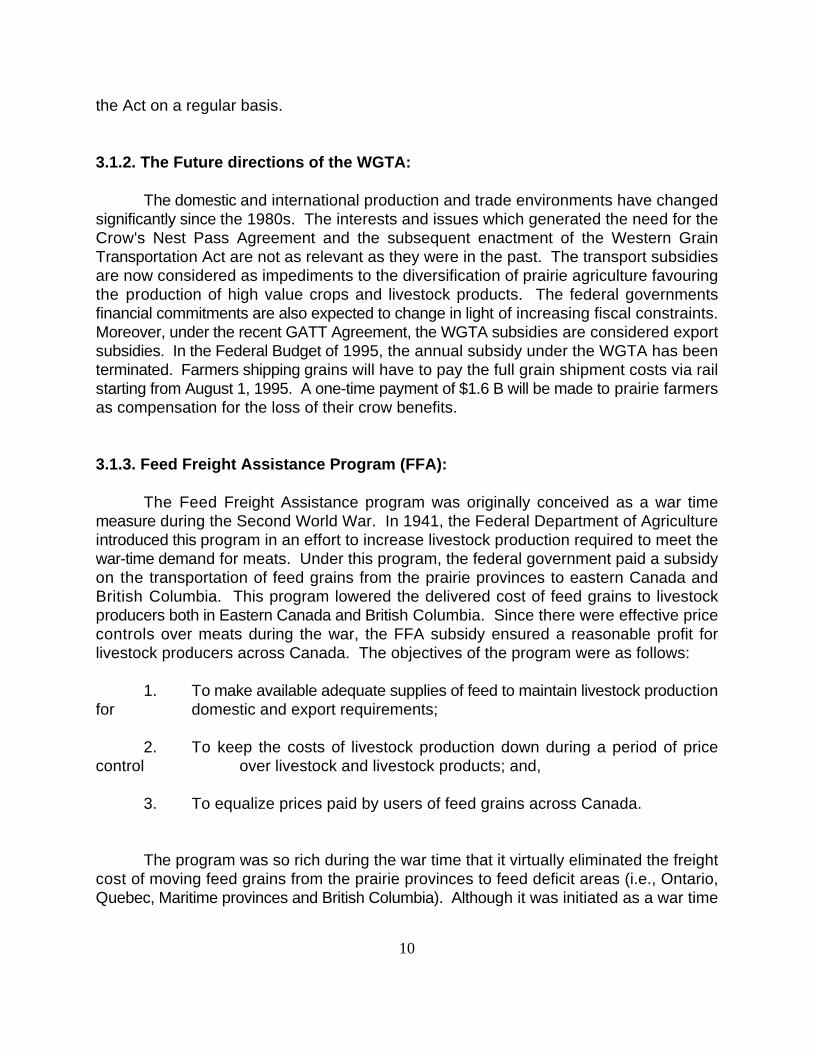
annual income to be supported throughout the country. If there is an agreement, however,it will go a long way to improve the financial viability of small and mid-sized family farmsin this country. Since a negative income tax is calculated based on one's whole farmincome, it is production and trade neutral and hence, could be considered 'GATT green'.A synoptic overview of various farm programs is given in Table 3.1.

3.2. Possible Future Directions of the Safety Net Programs for Agriculture:

In order to make domestic agricultural policies compatible with GATT regulationsthe current safety net programs for agriculture in Canada are expected to be redesigned.In this retooling process some existing programs may disappear and some new programsmay be introduced. The following are some of the policy issues which have beendiscussed in recent months:

1. The Gross Revenue Insurance Plan appears to be in trouble both economicallyand politically. Saskatchewan has already pulled out of the GRIP. Manitoba is expectedto exit as well. Alberta has also given a notice. As support levels under the GRIP decline,farmers in other provinces may find it less attractive, leading to a mass exodus from theprogram. The GRIP is also subject to our reduction commitments under GATT (1994)because of its production and trade distorting features. It seems likely that the federalgovernment will kill GRIP by the end of 1995. A whole-farm income insurance programhas been proposed as a replacement for GRIP. Under this program farmers will paypremiums into the program and will get payouts when farm income drops below their five-year average. However, farmers who get payouts will be defined as high risk and theirpremiums will go up. To avoid higher premiums, a farmer could withdraw money from hisNISA account to supplement income.

2. Another proposal calls for a stronger NISA in 1995. It would be a whole farmbased program for any agricultural product. The cost of the program would be shared bythe producers (50%), the federal government (33%) and the provincial governments (17%).The value-added form of NISA could be used instead of the currently available NISA.

3. In case market revenue insurance under GRIP is eliminated, an enhanced NISAcould replace it. Under this proposal, supply managed commodities could be included inthe program and the cost of the program would be shared by producers (50%), the federalgovernment (25%)

20

Table 3.1: An Overview of the Canadian Safety Net Programs for Agriculture

Program Starting Year Basic Features

Efficiency Implications for

Farm Production Input Supplies Processing Program Cost Risk &Sector Uncertainty

Western Grain Transportation Act 1983 - Freight rates are shared by the producers Increased for Increased Reduced High Reduced(WGTA) and the government; supported

- The government pays Crow Benefit worth commodities$659 million/year to railways;- Only the initial 31.5 mil. tonnes of grain receive subsidized freight rates;- Subject to our reduction commitments underGATT

Feed Freight Assistance (FFA) 1941 - Ensures adequate supplies of feed to Increased Increased Increased Low Neutrallivestock producers in deficit regions;- Equalizes feed grain prices across Canada;- Considered 'GATT Green'.

National Tripartite Stabilization 1986 - Commodity specific; Increased Increased Increased High ReducedProgram (NTSP) - Support based on a guaranteed margin;

- Costs shared equally by three parties;-Subject to our reduction commitments underGATT

Gross Revenue Insurance Plan 1991 - A form of tripartite stabilization program; Increased for grains Increased Increased High Reduced(GRIP) - Provides both price and yield protection; & oilseeds but

- Support based on target price and target reduced for othersyield levels;-Subject to our reduction commitments underGATT

Net Income Stabilization Account 1991 - Producers contribute 2% of eligible sales Neutral Neutral Neutral Moderate Neutral(NISA)[or Value Added Income (max. $5,000) matched by government Stabilization Account (VAISA)] contribution;

- Producers can contribute additional 20% of eligible sales (max. $50,000);- All producers' contributions earn 3% interest bonus;- Withdrawal can be triggered by a fall in either gross margin or net income below athreshold;- Considered 'GATT Amber'.

Negative Income Tax (NIT) Being discussed - No producer contribution; Neutral Neutral Neutral Low Neutral- Support based on net farm income;- Would be considered 'GATT Green'.

21

and the provincial governments (25%). If supply managed commodities are left out ofNISA, the general availability nature of NISA would be compromised under GATTregulations.

3.3 Decoupled Farm Programs:

Decoupled, production neutral and minimally trade distorting are all terms that havebeen added to the trade policy analysts lexicon in the past decade. While exact definitionsof these terms vary across analysts the basic concept is simple; income support tofarmers, which may be desirable on political grounds, should be provided in ways thatleave production, consumption and hence trade unchanged from its competitive level.

Magiera, et al. have defined a decoupled government payment as one where"neither the implementation nor removal of a payment has any effect on production ...(p.7)". Obviously, in order for the payment to be completely non-trade distorting, it shouldhave no impact on consumption. Using this strict definition of decoupling it is unlikely thatany payments targeted to the agricultural sector are completely decoupled since they allaffect the level of resources employed in agriculture, labour-leisure choices and/orproducers' risk attitudes.

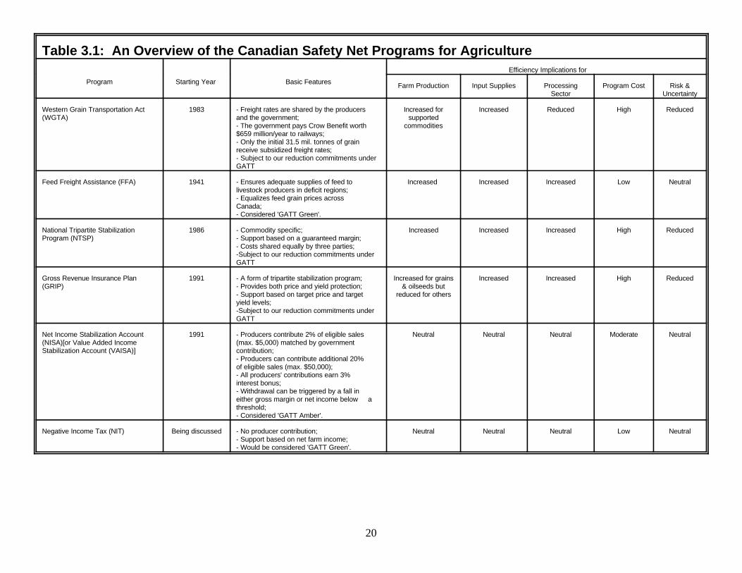
Although completely decoupled farm program payments are rare, there is little doubtthat some ways of providing farm income support are more production and trade distortingthan others. Magiera et al. categorized programs into six types, ranging from the least tothe most trade distorting (Table 3.2). It is useful to review these, noting at the outset thatthe discussion is focused on domestic policy options. Frontier measures, which arerequired for the successful implementation of some domestic policies, are seen as thenecessary outgrowths of these domestic policies. If the domestic policies are dismantledor reinstrumented in trade friendly ways, then there is little necessity for the bordermeasures.

Turning to Table 3.2, the least trade distorting type of program (level 1) is a programwhich is generally available across the entire economy and which requires no agriculturalactivity to obtain. These national policies are not controversial, at least in trade policyterms, and minimally distorting. All nations deem these policies to be politically sovereignand desirable in a modern society; they are not the focus of attention in trade liberalizationdiscussions.

Level 2 programs differ from level 1 programs in that they are available only to theagricultural sector. However, direct payments to individuals do not require the recipientto remain in farming to receive the program benefits. If the payments are tied to aresource, eg. land or labour, this resource is not required to remain in agriculture toreceive the payment. Even though these programs are targeted at the agricultural sector,

22

since agricultural activity is not required to receive benefits these policies should remainrelatively production neutral. Examples of level 2 programs might include early retirementbonuses paid to older farmers or per area payments used to achieve conservation orenvironmental goals, while not requiring continued use in agriculture.

23

Table 3.2: Characteristics of Agricultural Programs and the Level of Trade Distortion

Trade Descriptive Characteristics of Programs

Distortion Level ______________________________________________________________________________

Least Level 1 Available to AnyoneNo Agricultural Activity Required

Low Level 2 Available Only to Agricultural ProducersNo Agricultural Activity RequiredPayments Unrelated to Output/Input Use

Level 3 Available Only to Agricultural ProducersAgricultural Activity RequiredPayments Unrelated to Level of Output/Input Use

Level 4 Available Only to Agricultural ProducersAgricultural Activity RequiredPayments Related to Level of Output/Input Usebut With Limits on the Level of Output/InputReceiving Support

High Level 5 Open-ended Direct Payments Related to the Level of Output/Input Use

Most Level 6 Administered Prices Applicable to Total Output -Maintained with Border Controls and Involving aConsumption Distortion

______________________________________________________________________________

24

The degree of potential distortion increases sharply as programs move into the level3 category. In level 3, agricultural output is required to receive program benefits. This hasthe effect of holding land, labour and capital in the agricultural sector, and hence distortsproduction decisions. However, the fact that the benefits are not tied to the level of outputor input use serves to eliminate the incentive to expand agricultural production to increaseprogram rewards.

Most agricultural programs in Canada and elsewhere are level 4 or higher. Level4 programs link payments directly to the level of output or input use but restrict the size ofthe program benefits by limiting the quantity of output or input to which the subsidy applies.

Level 5 programs are the same as level 4 programs but the extent of governmenttransfers are open-ended. This provides an incentive to expand production to maximizeprofits, inclusive of the government payment. The larger and more certain this payment,and the more price elastic the producer's supply response, the more production and tradedistorting the program. Historically, Canada has had several programs of this type: theAgricultural Stabilization Act, the National Tripartite Stabilization Program and the GrossRevenue Insurance Program come immediately to mind.

The final category of programs (level 6) provides open-ended administrative pricesupports coupled with a consumption distortion, which requires border controls to beeffective. The Common Agricultural Policy of the European Union is of this type. Level5 and level 6 programs are the most distorting of those surveyed. These programs changeproducer's marginal revenue and marginal cost calculations and encourage them toexpand output in response to the availability of governmental subsidies.

One of the goals of the Uruguay Round of trade negotiations on agriculture was toprovide an incentive for countries to move away from the most trade distorting policies andtowards more trade friendly regimes. Unfortunately, no form of agricultural policy waseliminated. However, the constraints on export subsidies (both in volume and expenditureterms) and minimum access requirements will constrain countries use of the most highlydistorting programs. In addition, the discipline on domestic support, the identification of"green" programs, the desire to avoid countervailing duties, and individual countries owndesire to limit budget exposure will result, over time, in more trade friendly policies.

One issue addressed only indirectly in the work by Magiera, et al. is the effect ofgovernment policies that reduce the risk faced by primary producers. Welfare theorysuggests that government intervention can be justified where there are incomplete marketsin insurance and credit and agricultural producers are unquestionably subject to large andunpredictable market risks. Some risks can be hedged on organized future markets andfarmers can also self-insure through precautionary savings, but these tools typicallyprovide protection for only short periods.

25

The practical definition of decoupled income support is likely to be developedthrough multilateral trade negotiations. These are the rules that will provide the pragmaticanswer to whether a sovereign nation's agricultural policies are in conformity with thecommitments it has made in the GATT, and if these policies are countervailable. For thatreason it is useful to review what was decided in the Uruguay Round and how Canada'sagricultural policies stack up against these rules.

The GATT (1994) agreement on agriculture has adopted two general criteria todefine decoupled or "green" programs. Green programs are important because they arenot subject to the domestic support reduction requirements negotiated in GATT (1994) andin some cases are exempt from countervailing duty action.

The two general criteria were adopted for "decoupled" programs:

@ Support must be provided through a publicly funded programme notinvolving transfers from consumers; and

@ the support in question shall not have the effect of providing price supportto producers.

The GATT (1994) goes on to further define specific criteria that can be used toexempt certain types of support to the agricultural sector from negotiated reductions.These can be delineated into four broad groupings: (1) production or trade distortingsupport that falls below a de minimis standard; (2) support for general services which doesnot involve a direct payment to producers; (3) direct payments to producers coupled withsupply management; and (4) direct payments to producers not requiring supplymanagement. The criteria for each of these "green" program types is reviewed below.

3.3.1. De Minimis Standard:

GATT (1994) states that government support provided to individual agriculturalproducers and to the sector in general is considered minimally trade distorting if it meetsthe following criteria:

@ product specific domestic support where such support does not exceed 5 percentof the value of production; and

@ non-product specific domestic support where this support does not exceed 5percent of the total value of production.

These rules allow for some minimal support to all commodity sectors.

26

3.3.2. Support for General Services:

Support provided to the agricultural sector but not to individual producers is exemptfrom domestic support reductions if it involves: 1) research, 2) pest and disease control,3) training services, 4) extension and advisory services, 5) inspection services, 6)marketing and promotion services, 7) infrastructure services, involving off-farm capitalprojects; 8) public stockholding for food security purposes, and 9) domestic food aid.

Programs falling into this category would be classified as level 2 or level 3 programsin terms of their distortionary impacts (Magiera, et al.).

3.3.3. Direct Payments Involving Supply Management:

These programs, level 4 in terms of production and trade distortions, were includedin GATT (1994) to exempt certain forms of income support used in the EU and U.S. fromthe domestic support reduction commitments. Pragmatically, this "omission" wasnecessary to reach a successful conclusion to the Round.

The specific criteria state that direct payments made to producers are consideredminimally trade distorting if:

@ payments are based on a fixed area and yield; or

@ payments are made on 85% or less of the base level of production; or

@ livestock payments are based on a fixed number of head.

Interestingly, the degree of production restriction required to be considered underthese criteria in GATT (1994) is left unstated. Under certain conditions these programswould be consistent with the idea of a production entitlement guarantee (IATRC).

3.3.4. Direct Payments to Producers Not Involving Supply Management:

While open-ended direct payments to producers (level 5) are one of the mostdistorting forms of agricultural program the GATT (1994) has adopted criteria that allowsgovernments to give income support to producers under specified conditions whichexempts them from domestic support reduction commitments.

A number of program types are considered under this category. Structuraladjustment programs involving producer retirement programs, resource adjustmentprograms and investment aids are all allowed as long as the payments are not related to

27

current production, prices or input use. Likewise, payments for the relief from naturaldisasters, environmental programs and regional assistance programs are exempt subjectto certain conditions.

However, of most interest for this project are the criteria for decoupled incomesupport and acceptable government contributions to income insurance and safety-netprograms.

In order for GATT (1994) to consider income support to be decoupled, eligibility forpayments must be determined by clearly defined criteria during a base period. In addition,the amount of the payments should not be influenced by the type or volume of production,prices or the use of factors of production beyond the base period; and no productionshould be required to receive these payments. The authors are unaware of any seriouspolicy consideration being given to Canadian programs that would meet these criteria.

Of more interest are the criteria for income insurance and safety-net programs. TheGATT (1994) criteria for these programs are:

@ eligibility for payments based on income loss, which exceeds 30% of averagegross income (or the equivalent in net income terms) in the proceeding 3year period, or a three year average based on the proceeding 5 year period,excluding the highest and lowest entries;

@ payments should compensate for less than 70 percent of the income loss; and

@ the amount of payments should relate solely to income, not to type or volume ofproduction, prices of factors of production.

If NISA is extended to all commodities, it appears it could be redesigned to conformto these criteria. The empirical question is to what extent a GATT (1994) "green" safetynet program would stabilize farm income and consumption, the extent to which it would beproduction distorting, the political acceptability of such a program, the distribution ofbenefits from such a program and the transfer efficiency of such a program.

28

4. A GENERAL APPROACH TO MEASURING THE TRANSFER EFFICIENCY OFGOVERNMENT SUPPORT PROGRAMS

The measure of transfer efficiency must necessarily be identified by the incrementalbenefits associated with revenue enhancement and risk reduction. The very nature ofstabilization policies guarantee that the two attributes are not mutually exclusive and,therefore, ought not to be treated separately.

It is unreasonable to consider a farmer decision making process which excludessimultaneous consideration of risk and return, and this has implications for the assessmentof overall transfer efficiency. The following working definitions of risk reducing stabilizationpolicies identify this importance.

1) Risk reducing policies: A risk reducing policy is one in which governmentstabilization policies are defined in terms of a specific payout or indemnity related in somefashion to a pre-specified target price and the actual cash commodity price at a specificmoment, or specific moments, in time.

2) A pure stabilization policy is one in which producers direct (e.g. premiums) orindirect (e.g. set-aside or compliance) costs equal the expected benefits of the stabilizationpolicy. Such a policy is actuarial sound and is thus revenue neutral.

3) A revenue enhancing policy is one in which farmers' costs of participation areless than the actuarial value of the program. In this instance, expected revenueenhancement occurs and is equal to the difference between the farmer's actual cost andthe actuarial cost of participation.

While risk reducing transfer policies can, under some circumstances (actuarialsoundness), be deemed revenue neutral (expected benefits equal expected costs), it is nottrue that, under conditions of risk, revenue enhancing policies are not risk reducing. Thisis clear in definition (3) above for stabilization policies such as NTSP, ASA or GRIP. Evennon-targeted policies (such as lump-sum transfers, input subsidies, freight assistance, etc.)which do not affect risk directly can result in a variance preserving shift in expectedincome. When measured relative to a fixed target, lump sum transfers and other decoupledprograms will reduce the chance of actual income falling below the target and cantherefore, lead to increased output. These programs will also affect input demand.

The remainder of this section details a theoretical approach to measuring the costsand efficiencies of transfer programs and transfer efficiency in this context. Thisbackground will then be used as the basis for developing a farm-level optimization modelwhich will identify portfolio shifts as a result of a variety of stabilization policies. Theseportfolio shifts will then be used to approximate and identify the transfer efficiency ofstabilization programs.

29

4.1. The Firm's Response to Uncertainty:

Because the majority of risks in agriculture arise from prices and yields mostpolicies have been directed towards stabilizing them. In this section three models of thefirm's response to uncertainty are presented. The first two models are simple, based ona mean variance expected utility approach of the farm firm, under perfectly competitiveconditions (i.e. price is exogenous). The third model also assumes perfect competition butdiffers in that it is used to examine the portfolio effects of stabilization policies. In all 3models the focus is on output response to risk.

4.2. Output and Price Uncertainty:

In this section a simple model of production when yields are assumed deterministicbut prices are random is used to evaluate the farm's response to price risk. It is assumedthat farmers are risk averse. Under conditions of risk aversion, it is shown in Appendix Athat:

When product prices or commodity yields are risky, farmers willproduce below the profit maximizing level of output.

As shown in Appendix A, risk averse farmers will not optimize by setting marginal revenuesequal to marginal costs, but will set marginal revenues equal to marginal costs, minus adeduction for marginal risks. This latter deduction represents the marginal incomeforegone to obtain more stable returns.

The impact of risk on output is shown in Figure 4.1. The farm's average cost curveis AC while MC' and MC represent the farmers marginal costs under conditions of risk andcertainty respectively. The difference between the two marginal cost curves is attributedto farmer's risk perception. The risk premium, on the margin, is given by the verticaldistance between the two marginal cost curves.

The result is that output is lower under conditions of risk and so are net revenues.Given that total variable costs are given by the area under the MC curve, expected netrevenues are reduced by the area abc due to risk aversion.

4.3. The Effect of Price Insurance and Stabilization:

The major goal of government programs is to reduce income fluctuations and thisis done to a significant extent by stabilizing prices such as in the Agricultural StabilizationAct or providing price insurance such as market revenue insurance (GRIP) and theNational Tripartite Stabilization Policy.

The curve in Figure 4.2 represents the relationship between random prices and

30

price insurance. The bell shaped curve is the probability distribution function, f(P), whichdescribes the universe of possible price outcomes. The mean is given by P and risk ism

measured as a deviation from this mean.

31

Figure 4.1

32

Price insurance or stabilization provides a benefit to producers by `stacking'probabilities of outcomes below a target price, at the target price. For example in Figure(2), the density function is truncated at the target price P , such that the probability ofz

getting below P is zero. For example, if the market price is at P , the farmer receives anz o

indemnity equal to P -P as part of the stabilization payment.z o

The expected benefits from stabilization/insurance policies are equal to theexpected payouts across all states of nature. This relationship is shown mathematicallyin Appendix B. In agriculture, policy is not designed to charge farmers an actuarialpremium for the benefits of stabilization or insurance policies. The, now defunct,Agricultural Stabilization Act did not require producer contributions, whereas NTSP andGRIP charge a premium equal to 33% of the expected value of the policy. In the U.S.,participation in the target price-loan program requires cross compliance with conservationpolicies and land set-aside which also results in some costs being levied against thebenefits.

Stabilization policies have two, not mutually exclusive impacts on farm decisionsand transfer efficiency. The first deals with the subsidization of premiums, which is incomeenhancing, while the second deals with risk reduction. The impact of premiumsubsidization and risk reduction is derived mathematically in Appendix B. The key resultsare:

1) When farmers pay a less than actuarially fair price for agriculturalinsurance, marginal revenues per unit of output, increase, leading toincreased output;

2) the effects of risk reduction reduces the disutility associated with risk, andthe opportunity costs of risk bearing. This in turn leads to increased output,relative to the no policy case; and

3) the effects of income enhancement and risk reduction mitigate each otherso that output increases even more when both aspects of agricultural policyare present.

This is shown in Figure 4.3 where output will increase because marginal revenueshave increased and the risk premium has decreased.

The reduction in risk causes the marginal cost curve to become flatter, moving itfrom MC to MC , and increasing output from Y to Y , increasing expected net revenueso 1 o 1

by an amount equal to the area abc. This is termed the risk reduction effect and is directlyattributable to the risk reduction policies of agricultural insurance.

Farmers will view the premium subsidy on price insurance and stabilization as anincrease in marginal revenues so output increases along the new marginal cost curve MC1

from b to e, increasing output from Y to Y , and net profits by the area abed compared to1 2

the net profit without premium subsidy. This is termed the income effect, and is directly

33

attributable to the subsidization of agricultural insurance.

34

Figure 4.2

35

Figure 4.3

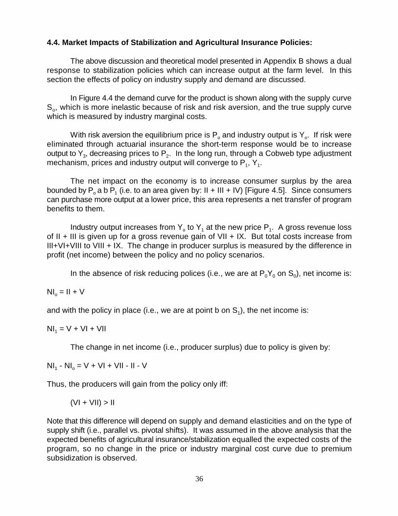
36

4.4. Market Impacts of Stabilization and Agricultural Insurance Policies:

The above discussion and theoretical model presented in Appendix B shows a dualresponse to stabilization policies which can increase output at the farm level. In thissection the effects of policy on industry supply and demand are discussed.

In Figure 4.4 the demand curve for the product is shown along with the supply curveS , which is more inelastic because of risk and risk aversion, and the true supply curveo

which is measured by industry marginal costs.

With risk aversion the equilibrium price is P and industry output is Y . If risk wereo o

eliminated through actuarial insurance the short-term response would be to increaseoutput to Y , decreasing prices to P . In the long run, through a Cobweb type adjustment3 2

mechanism, prices and industry output will converge to P , Y .1 1

The net impact on the economy is to increase consumer surplus by the areabounded by P a b P (i.e. to an area given by: II + III + IV) [Figure 4.5]. Since consumerso 1

can purchase more output at a lower price, this area represents a net transfer of programbenefits to them.

Industry output increases from Y to Y at the new price P . A gross revenue losso 1 1

of II + III is given up for a gross revenue gain of VII + IX. But total costs increase fromIII+VI+VIII to VIII + IX. The change in producer surplus is measured by the difference inprofit (net income) between the policy and no policy scenarios.

In the absence of risk reducing polices (i.e., we are at P Y on S ), net income is:0 0 0

NI = II + V o

and with the policy in place (i.e., we are at point b on S ), the net income is:1

NI = V + VI + VII1

The change in net income (i.e., producer surplus) due to policy is given by:

NI - NI = V + VI + VII - II - V1 o

Thus, the producers will gain from the policy only iff:

(VI + VII) > II

Note that this difference will depend on supply and demand elasticities and on the type ofsupply shift (i.e., parallel vs. pivotal shifts). It was assumed in the above analysis that theexpected benefits of agricultural insurance/stabilization equalled the expected costs of theprogram, so no change in the price or industry marginal cost curve due to premiumsubsidization is observed.

37

38

Figure 4.4

39

Figure 4.5

40

However if premiums are subsidized then the shadow price increases from P to Po o

+ (1+*)V over an output )Y, which we assume equal to the initial equilibrium level of output.

When producers view premiums subsidization as an increase in price then bothprice and output will fluctuate widely in the short-run. This will happen because the pricesignal received from the policy differs from that received from the market. For example,in Figure 4.6, P + *V is the price. At this price the signal is to increase output to Y . But1 1 2

at Y consumers are only willing to pay P . In the next response iteration, the price is P2 3 3

+ *V and output is reduced to Y . At this lower level of output consumers are willing to3 3

pay a higher price, and the price increases signalling an expansion of output.

Ultimately if subsidization is viewed as an increase in notional price an equilibriummay not be obtained and output and prices become, in the long run very unstable, andvariance may actually increase with divergent oscillations between low output and highprices and high output and low prices. These models are based on the assumption of aclosed economy. The impacts would be much less severe with international trade. If,indeed, competitive import and export markets exist, then net transfers to farmers willincrease.

If producers view the subsidy as a decrease in marginal costs then a stableequilibrium can be found, as shown in Figure 4.7. In Figure 4.7, the industry MC curveshifts from S to S and output increases from Y to Y while prices decrease from P to P .1 2 1 2 1 2

The transfer of income to producers through subsidized premiums will ultimately end upas a gain to consumers through an increase in consumer surplus. The extent of gain willbe lower if the policy is coupled with supply restrictions or other compliance measures.While such restriction can lead to an increase in benefits transferred to farmers it comesat a cost to society as a whole.

4.5. The Transfer Efficiency of Crop Insurance:

Crop insurance is offered in many forms to farmers across Canada. Provinciallyadministered, and financed by provincial, federal and farm contributions, it has been widelyadopted by farmers and, unlike many of the price based insurance/stabilization policies,has remained fairly consistent over time.

Like price insurance the effect of crop insurance is to truncate downside yield risks.However, the nature of risk reduction and the marginal risk response is slightly different,and is derived in Appendix C. Like price insurance, crop insurance reduces risk bytruncating the variance of yields. If insurance is offered on an actuarial basis then themarginal cost curve becomes flatter (more elastic) and an overall increase in output canbe observed.

In Figure 4.8, MC is the marginal cost adjusted for risk premium and is represented0

by a solid line. The marginal cost curve MC represented by the dashed line would have2

been the actual marginal cost curve in absence of risk. Thus, if an actuarial priced

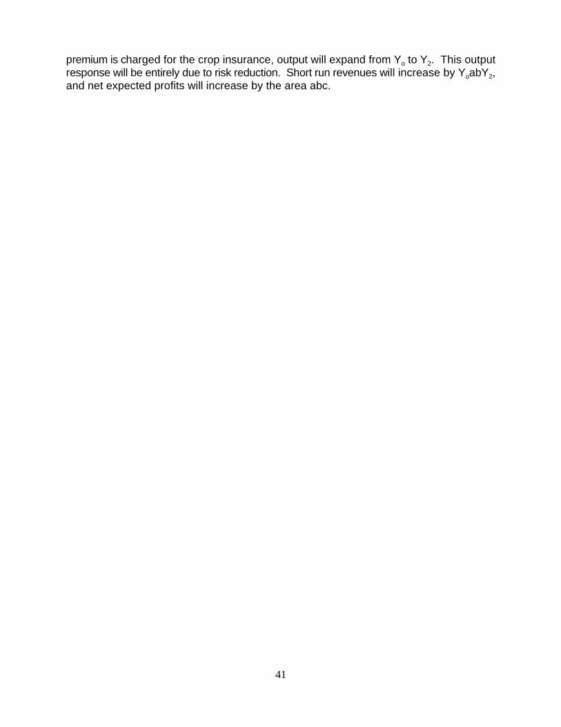
41

premium is charged for the crop insurance, output will expand from Y to Y . This outputo 2

response will be entirely due to risk reduction. Short run revenues will increase by Y abY ,o 2

and net expected profits will increase by the area abc.

42

Figure 6

43

Figure 7

44

Subsidizing crop insurance premiums can also have an effect on output. This isshown in Figure 4.9. Depending on the nature of risk and degree of premiumsubsidization, output will increase from Y to Y . Without insurance, marginal profit is2 3

given by the area Pao. With actuarial priced insurance, output increases to Y and2

marginal profit increases by the area abc. Finally, with subsidized premiums the marginalcost curve shifts to the right, output increases to Y , and net profits increases by an area3

cde.

4.6. The Market Effects of Crop Insurance:

As in the price insurance/stabilization case crop insurance can have an impact onprices at the aggregate level. This is shown in Figure 4.10.

In the absence of risk aversion, production is at Y and the market price is P . Theo o

introduction of crop insurance will, in the short run, increase output to Y due to the risk2

reduction effect, and to Y due to the income (subsidy) effect. In the long run, as markets3

adjust to excess supply conditions following a cobweb type adjustment procedure,unsubsidized insurance would result in output at Y and a price P , and when subsidized,1 1

equilibrium results in output Y at price P .2 2

Without crop insurance, consumer surplus is given by area a and producer surplusis given by b+e+j (Figure 4.11). Risk reduction with actuarial premiums increasesconsumer surplus by b + c + d. Producer surplus decreases by b + c + d but increases byf+g+k. If the objective of policy is to transfer benefits to producers through stabilizing risks,it is unlikely that producers will be the primary beneficiary. The greatest gain may go toconsumers.

Finally, the effect of subsidizing premiums is to increase output and decrease pricefurther (to P and Y ). Consumers gain e+f+g+h+i which is a loss to producers, but2 2

producers also gain an area represented by l+m+n.

4.7. Discussion on the Transfer Efficiency of Agricultural Insurance Policies:

The previous discussions focused on two aspects of transfer programs. It assumesthat producers are initially risk averse and due to this risk aversion output is reduced belowits socially optimal level.

To combat this, public policy provides an array of transfer programs to help farmers.These programs do two things: first they reduce risk and second they increase expectedreturns.

While the impact on consumers is clear - they benefit by having lower prices onmore output - the impact on farmers is less obvious. Factors which affect producer surplusor enhanced net income are the relative elasticities of supply and demand. If the demand

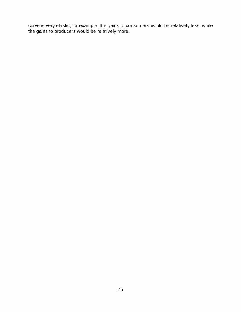
45

curve is very elastic, for example, the gains to consumers would be relatively less, whilethe gains to producers would be relatively more.

46

Figure 4.8

47

Figure 4.9

48

Figure 4.10

49

Figure 4.11

50

Collectively both price insurance and crop insurance used together can lead to asignificant increase in output. The absolute change in output, and the intermediate tolong-term market impacts depend on the elasticities of supply and demand. If supply isfairly inelastic the inevitable outcome is that it becomes less inelastic, but the change maynot be so great.

The impact on market prices will, in the intermediate to long-run, result in adecrease in domestic prices, with the greatest reduction occurring for inelastic demands.Domestic price changes will, however, be dampened if an export market exists to absorbsome of the excess supply.

4.8. The Impact of Stabilization Programs on Input Demand and Input Markets:

Under classical assumptions input demand is a function of output and the relativeprices of inputs, while supply is a function of commodity prices and input prices. Throughthe economic relationships (vis a vis Hotellings Lemma) between the cost function and theprofit function input demand can be expressed as a function of output prices and inputprices.

As shown in Appendix D, the response in input use to an increase in expectedmarginal revenues will increase the demand for agricultural inputs. The result implies anoutward shift in the input demand curve in response to a change in expected output pricedue to insurance. Costs to producers increase by the area W (X -X ) which is a directo 1 o

increase in revenue to suppliers.

In the intermediate to long-run input supply will increase to meet the excess demandand input prices will increase.

The adjustment response to agricultural insurance is thus an increased use ofinputs and an increase in price. Producer's costs ultimately increase by W X -W X for1 2 o o

total costs of W X .1 2

Revenues to input suppliers increase from W X to W X , but total costs increaseo o 1 2

by the area below the supply curve and bounded by X and X . Thus the direct effect of2 o

subsidized agricultural insurance in which dP > 0 is to increase costs to farmer andrevenues to input suppliers. The degree by which the input demand curve shifts outwardsdepends also on farmer's degree of risk aversion and the response to risk.

4.9. NISA and Whole Farm Programs:

The economics of a NISA type program has not previously been determined. NISAand VAISA type programs have been designed to encourage self reliance in meetingliquidity requirements when adverse economic conditions prevail.

51

One approach to investigating the economic consequences, and transfer efficiencyof NISA is to view the problem in the context of a savings-consumption problem rather thana production problem. This view is based on the premise that farm households are prudentin that they are willing to set aside current consumption as precautionary savings forstabilizing future consumption.

With NISA the transfer efficiency of funds are measured in terms of the matchinggovernment contributions, and the interest rate premium received on (eligible) depositedfunds. The problem is to determine whether or not the transfer of these funds results inportfolio and production effects, as a result of increased risk taking.

4.10. A Simplified Approach to the Analysis of NISA and NISA Type Programs:

The introduction of whole farm insurance is a new concept in delivering public policyprograms. There are, in essence, two distinct forms of whole farm insurance. The first iswhole farm income insurance which provides a payout to farmers if income from operationsfalls below 70% of income from the previous years, averaged. These programs affectoutput by truncating the variance of the farm crop portfolio directly. Farmers' response tothe program is based primarily on the policy parameters such as target incomes, and theamount by which portfolio variance can be reduced through truncation. A rationalresponse to whole farm income insurance is to substitute less risky crops with more riskyones. The amount of substitution depends on the target income level (e.g. 70% or 85%)and the amount by which the actuarial value of the program is subsidized. The movetowards higher risk and return opportunities will increase with increased coverage levelsand subsidies. However, since the actuarial value of portfolio insurance increases, it isunlikely that such a program will encourage an otherwise risk averse farmer to behave asa risk neutral, profit maximizing farmer. The reason for this is that the marginal increasein risk, and hence premiums, will at some point exceed the marginal increase in expectedbenefits. At this point it would no longer be rational for the farmer to substitute for furtherrisk increases.

In contrast to whole farm insurance, NISA and NISA type programs, have amechanism which works through a savings account. In years in which net income (neteligible sales) exceeds historic income, money is deposited into an interest earningsavings account which earns a premium rate, and deposits are matched by thegovernment. For years in which net eligible sales are less than the historic averagefarmers can withdraw from the NISA account to make up the difference.

The mechanics of NISA has the appearance of separating savings/consumptionpatterns from production. Because withdrawal in poor years is not mandatory, the likelyconsequence is that NISA is viewed as a buffer to stabilize variability in consumption,rather than farm income per se. Because savings-consumption patterns are separatedfrom production decisions by time, NISA type programs will have only a modest impact onproduction decisions. As shown below, factors which can possibly impact productiondecisions are the perceived correlation between production and savings; the subjective

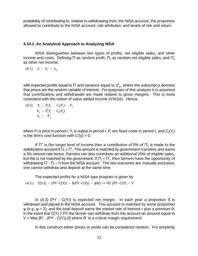
(4.1) B ' B1 % B2

(4.2) Bt ' PtYt & Ct(Yt) & Ft

B1 ' PtYt & Ct(Yt)B2 ' &Ft

(4.3.) E[B)] ' (PY&C(Y)) & *(PY&C(Y)) % R*(1%r%2) (PY&C(Y) % V

52

probability of contributing to, relative to withdrawing from, the NISA account; the proportionallowed to contribute to the NISA account; risk attributes; and levels of risk and return.

4.10.1. An Analytical Approach to Analyzing NISA

NISA distinguishes between two types of profits, net eligible sales, and otherincome and costs. Defining A as random profit, A as random net eligible sales, and A1 2

as other net income,

with expected profits equal to )A and variance equal to F , where the subscript p denotes2p

that prices are the random variable of interest. For purposes of this analysis it is assumedthat contributions and withdrawals are made relative to gross margins. This is moreconsistent with the notion of value added income (VAISA). Hence,

where P is price in period t, Y is output in period t, F are fixed costs in period t, and C (Y )t t t t t

is the firm's cost function with C'(y) > 0.

If A is the target level of income then a contribution of *% of A is made to the*1

stabilization account if A > A . This amount is matched by government transfers and earnst*

a 3% interest rate bonus. Farmers can also contribute an additional 20% of eligible sales,but this is not matched by the government. If A < A , then farmers have the opportunity oft

*

withdrawing A - A $ 0 from the NISA account. The two outcomes are mutually exclusive;*t

one cannot withdraw and deposit at the same time.

The expected profits for a NISA type program is given by

In (4.3) (PY - C(Y)) is expected net margin. In each year a proportion * iswithdrawn and placed in the NISA account. This account is matched by some proportionR (e.g. R = 2), and the total deposit earns the market rate of interest r plus a premium 2.In the event that C(Y) > PY the farmer can withdraw from the account an amount equal toV = Max [R - (PY - C(Y)),0] where R is a critical margin requirement.* *

In this construct either prices or yields can be considered random. For simplicity

(4.4.) E(B) ' (PY&C(Y)) (1%*(R(1%r%2)&1)) % v

(4.5.) F2 ' Y2(1%*(R(1%r%2) & 1))2 F2p % F2

v& 2DpvY(1%*(R(1%r%2) & 1))FpFv .

(4.6) U(B) ' (PY&C(Y)) *( % V &82

(Y 2*(2F2

p % F2v & 2DpvY*

( FpFv)

(4.7) MU(B)MY

' (P&C )(Y)) *( & 8Y(Y*(2F2

p & *( DpvFpFv)

(4.8) Y ( '(P&C )(Y)) *(

8(*(2F2

p & *(DpvFpFv)'

(P&C )(Y))

8(*(F2p & DpvFpFv)

53

it is assumed that only prices are random. Since prices are random and stochastic, aNISA-type program has the interesting attribute that farmer's contributions are stochastic,since they depend on P, and consequently accumulated savings are random.

Expected returns (equation (4.3)) can be rewritten as,

and its variance is given by,

In (4.5) variance increases with respect to all of the policy parameters includingowner contribution, government matching, and interest rates. This increase in varianceis a direct result of the fact that savings and savings-investment earnings are stochasticallyrelated to price uncertainty. The term F is the variance of withdrawals from the NISA2

v

account. It too is a random variable which depends on the outcome of P. Its relationshipto P is measured by the covariance term in Equation (4.5), where D is the correlationpv

coefficient between NISA withdrawals and random prices. D will always be non positivepv

since an increase in withdrawals is triggered by a fall in prices. If farmers contribute toNISA, but never opt to withdraw then this correlation coefficient will equal 0.

Defining * = (1 + * ( R ( 1 + r + 2) - 1)), the expected utility is given by*

First order conditions yield

and,

There are several simplifications in this attempt to derive a tractable model forempirical measurement of the effect of NISA. For example, it is possible that there is aresponse MV/MY and MF /MY in which output levels affect the expected withdrawals and thev

2

variance of those withdrawals. It is, however, unlikely that this should occur in practicesimply because risk is captured through price variability, and most of this affect is capturedthrough the price-savings covariance. Also, as long as expected growth in savings exceedwithdrawals, it is unlikely that the incentives would exist to purposefully manipulate savings

(4.9)MY (

M*('

&(P&C )(Y))F2p

8(*(F2p & DpvFpFv)

2# 0

(4.10) Y ( '(P&C )(Y))

8F2p(*

( & DpvFpFv) / F2p

'P&C )(Y))

8F2p(*

( & $pv)

54

withdrawals.

From Y the effect of * is to increase output through its risk reducing effects;* *

Therefore, it must be true that MY /MR < 0, MY /Mr < 0, and MY /M2 < 0. On the surface* * *

these results do not appear to be intuitive. However, what they imply is that as *,R,r, and2 increases they become relatively more important in maximizing expected utility. Assavings and potential earnings from savings increase, it is optimal to reduce risk in orderto enhance the expected benefits from the NISA account. In a more general problem ofportfolio choice this result would imply that in order to stabilize contributions to the NISAaccount, and hence returns to the NISA account, farmers would diversify out of high riskcrops and into low risk crops. The result parallels an investment strategy in which wealthis transferred out of risky assets and into risk free investments as the benefits of risk freeinvestments increase relative to risky investments.

This diversification or reduction in revenue risk is mitigated by savings, and thecorrelation between price risk and withdrawals. Differentiating Equation (4.8) with respectto D yields M Y /M*MD $ 0, which implies that the more highly correlated are withdrawalspv pv

2 *

to price risk, the greater the output. A high correlation would indicate a high frequency ofwithdrawals, and hence the savings incentive is somewhat diminished. A correlation equalto zero would imply that the NISA account is being used as a pure savings account, andis not used to buffer consumption.

An alternative approach to assessing NISA type programs using Equation (4.8) as

where $ is the least square regression coefficient of withdrawals regressed againstpv

output prices. Since Y $ 0, i.e. output must be non-negative, then it must be true that ** *

> *$ *. Here *$ * can be defined as the absolute value of MV/MP, the rate at which NISApv pv

withdrawals change with respect to a change in prices. With a 2% eligible salescontribution, matching contributions from government, and interest rate plus subsidy ofabout 9%, * = 1.0226, so for positive output response with NISA stabilization, *$ * must*

pv

be less than 1.0226.

Finally the above assumes that there is sufficient liquidity in the NISA/VAISAaccount. The balance in the account is equal to the annualized future value of expectedNISA account balances, i.e.

(4.11) St ' S (1 % r % 2)t&1

r % 2

(4.12) Vt # S (1 % r % 2)t&1

r % 2.

55

where )S is the average or expected savings available. A necessary condition for the aboveresults to hold is that

Quite clearly, if expected withdrawals are greater than the NISA account balance,then the liquidity provided by the NISA account is inadequate to induce any outputresponse and producers will maintain a higher level of output and risk.

From the analysis herein it does appear that some aspects of NISA may not bedecoupled from production. The critical variable most likely to increase output is *, thefarmers contribution to the NISA account. As might be expected, the larger the allowablecontribution the larger the increase in output. This response will be lower for more riskadverse individuals and high risk crops. It is interesting to note that since commodityvariance is not truncated, as in the commodity specific programs, signals related to riskand return are maintained.

If any output effect is observed with NISA then it must be due to the relationshipbetween savings and consumption. However, output response will not generally bedirected towards higher risk - higher profit crops. Rather, the more likely response is toincrease production of low risk and low return crops. Furthermore, any effect would notoccur initially but only as riskless savings increase. If riskless savings are uncorrelatedwith risky production decisions there is an opportunity to increase risk taking activity, withthe safe investment being used to leverage increased risk. However, this effect isdependent on the amount of funds in the NISA account. For example, if market revenuesfor crops sold increase over time then so will deposits and accumulated deposits in theNISA account. However, if consumption smoothing exists when markets are volatile therewill be sufficient uncertainty in the NISA account balance to dampen any incentives toincrease production risks.

The implication is that funds transferred to farmers through the NISA program willnot be transferred to other agents in the agri-food sector. At most NISA savings would beused to satisfy payable accounts on expenses used in production but NISA in itself wouldnot cause those expenses to be incurred.

4.11. Summary and Conclusions:

56

This section has developed theoretical models related to commodity specificagricultural insurance policies and examined them within the context of transfer efficiency.

With respect to agricultural insurance the following results pertain:

1) Farmers participating in programs such as GRIP or NTSP will respond to reducedrisk by increasing output. This result follows from theoretical arguments which assign a riskpremium to risk averse behaviour. This premium is a function of risk, and decreases withrisk reduction. With respect to agricultural policies risk is reduced through truncation of theunderlying probability distribution.

2) When premiums are subsidized there is a greater output response. In general,subsidized premiums can be viewed as an increase in marginal revenues. As marginalrevenues increase relative to marginal costs (including the risk premium) new equilibriaare established at outputs levels higher than what would have occurred without them. Thesame general results hold for crop insurance.

3) As output increases so does the demand for inputs. Risk reduction, and orpremium subsidization tends to make the supply curve more elastic. In response to thismarket prices to consumers fall, although this may not be sustainable in the long run asmarkets adjust. In fact, in the situation where producers view subsidies as a premium, anequilibrium can never really be achieved as market signals become mixed with revenueincreases due to premium subsidies. If, however farmers view premium subsidies as areduction in marginal costs, then a long term stable equilibrium for market prices andsupply can ultimately be determined.

4) Agricultural insurance in general, and price insurance in particular, leads to anincrease in expected revenues. This has a direct impact on input demand to satisfyincreased output. The result is a transfer of program benefits to the suppliers of inputs, andan increased cost to farmers.

The neutrality of commodity specific programs is questionable. However, oneshould be cautioned about making broad statements in regards to whether all policies fallinto the GATT 'amber' category. There are two responses to stabilization. The first isthrough risk reduction. Farmers' response to risk reduction is a natural one and should notbe considered an 'amber' response if in fact premiums are actuarially fair. For example,farmers will behave in a similar fashion to selection of options on futures contracts as arisk management tool.

The problem in regards to GATT and other trade agreements is in the subsidiesassociated with these policies rather than the policies themselves. Farmers' response tosubsidies is an income effect which exacerbates any output response from risk reduction.Importantly, any challenge to these programs should be targeted only to the incrementalresponse to the income effect, not the risk reduction effect.

5) Since the gains from incremental risk taking are high relative to the possible

57

increase in NISA contributions it is unlikely that NISA will encourage risk taking activities.On the contrary, as allowable contributions increase they become relatively more importantin the economics of production process. As these savings become more importanteconomically, farmers will have the incentives to decrease revenue risks. This could beachieved through reduction in output or through diversification into lower risk crops. If thediversification strategy is used an increase in low risk crop production may be observed.Because of the relatively low contributions (2%) required for the NISA (or VAISA) accountit is unlikely that any portfolio shifts will be significant from a macro economic perspective.Furthermore, any response will likely be dampened if NISA withdrawals are highlycorrelated with decreased prices (or yields).

(5.1) Q ' Ga "b $

(5.2) Pa ' (P%S) "Ga "&1 b $

(5.3) Pb ' (P%S) $Ga " b B&1

(5.4) P % (1&*)V ' C )(Y) % 8YF2T

(5.5) E(U) ' PQ & aPa & bPb &82

Q 2F2p

58

5. FRAMEWORK FOR INVESTIGATING TRANSFER EFFICIENCY

5.1. Incorporating the Stabilization Model Framework into the Deloitte and ToucheFramework:

This section provides an approach to incorporating the stabilization framework intothe Deloitte and Touche framework. As discussed earlier, the theoretical model is general,and holds for NTSP, ASA, GRIP or any other program which provides commodity specificsupport. The foregoing is developed as a prototype for a single commodity only, and assuch should be adaptable to the Deloitte and Touche Framework.

The first 3 equations of the Deloitte and Touche framework are given by:

where Q is output, G is a constant, a is the level of farmer owned inputs, " its productioncoefficient or elasticity, b the level of purchased inputs, $ its production coefficient orelasticity, P is the price of farmer owned inputs, P the commodity price, S the level ofa

subsidy, and P the price of purchased inputs.L

From previous sections of this report, and Appendix B the first order condition fora risk averse producer in the presence of risk reducing stabilization policies if given by,

where * is the percentage subsidy, V the actuarial cost and benefit of agriculturalinsurance, C'(Y) is the marginal cost of output, 8 is the risk aversion coefficient, Y is outputor yield (Y = Q/a), and F is truncated variance.T

2

To maintain consistency with the Deloitte and Touche model, Equation 1 inAppendix A can be used to replace Equation 1 in the Deloitte-Touche framework. Thisyields a utility function of

This form of the Deloitte Touche model assumes that 8 is the average risk aversion

ME(U)Ma

' "PGa "&1b $ & Pa & "8QGa "&1 b $ F2p

ME(U)Mb

' $PGa " b $&1 & Pb & $8QGa " b $&1 F2p

(5.6) Pa ' "Ga "&1 b $ (P&Q8F2p)

(5.7) Pb ' $Ga " b $&1 (P&Q8F2p)

(5.8)MPa

Ma' "("&1) Q

a 2(P&Q8Fp) &

Q 2

a 28F2

p "2 < 0

(5.9)M2Pa

MaM8' &"("&1)

Q 2

a 2F2

p & "2 Q 2

a 2F2

p > 0 if " > 1/2

(5.10) Pa ' "Ga "&1 b B (P%S&28QF2p)

(5.11) Pb ' $Ga " b B&1 (P%S&28QF2p)

59

coefficient of producers, and that Q is aggregate output.The first order conditions are given by,

and,

In an economy without any subsidies (5.6) and (5.7) would capture the outputeffects of a risk averse economy. The impact of risk is to dampen demand for inputs. Forexample,

which in turn implies that risk averse producers will use less of the input than (say) riskneutral producers.

5.2. Transportation and Ad Hoc Subsidies:

The basic Deloitte-Touche model assumes a subsidy which is independent of risk.Transportation subsidies, and ad hoc deficiency payments would fall into this category ofsupport. The only impact this has on the model is to add to the output price, i.e. (P+S)rather than P, and Equations (5.6) and (5.7) become

Risk under risk aversion will still dampen input demand and lower output, but theimpact of including S is to shift the demand curve outward. Thus input demand will

(5.12) Pa ' "Ga "&1 b $ (P%(1&*)V & 2Q8F2T)

(5.13) Pb ' "Ga "&1 b $ (P%(1&*)V & 2Q8F2T)

(5.14)MPa

M*' &"Ga "&1 b $V # 0

(5.15)MPa

Ma' ("&1)Ga "&2 b $ (P%(1&*)V & 28F2

T) < 0

(5.16)M2Pa

MaM*' & ("&1)Ga "&2 b $V $ 0

(5.17)M2Pa

MaM8' & 2("&1)Ga "&2 b $V $ 0

60

ultimately be higher than the case without subsidy, but will still be lower than that predictedfor a risk neutral economy.

5.3. Stabilization Programs:

Stabilization programs differ from transportation or ad hoc subsidies because theyreduce risk by truncating the variance, and increasing expected revenues through premiumsubsidization. On an actuarial basis (1-*)V is the net benefit of the program which equalsthe actuarial premium, and * is the actual premium paid by the producer i.e. (1 - *) is thelevel of subsidy). The risk effect is such that F > F where F is truncated risk.p T T

The input demand equations for a stabilization program defined by

Two impacts that such programs have on input demand and output are premiumsubsidization and risk reduction. The effect of increased subsidy is given by

indicate that all other things being equal, an increase in * (i.e. farmer pays more of thepremium) the shift in the demand curve will be less, and demand will decrease.

(5.18)M2Pa

MaMFT' & 28("&1)Ga "&1 b $V $ 0

(5.19) Maximize EU(B) ' (PQ&aPa&bPb)*(

% V &82

[Q 2*(2F2

p % F2v % 2Q*(DpvFpFv]

(5.20) Pa ' "Qa

[P & 8(Q*(F2p % DpvFpFv)]

(5.21) Pb ' $Qb

[P&8(Q*(F2p % DpvFpFv)]

61

Equations (5.15) through (5.18) show how demand changes along the demandcurve. Equation (5.15) shows that the demand curve is downward sloping. Equation (5.16)shows that the impact of a subsidy on actuarial premiums (i.e. a decreasing) results in anincrease in the demand for inputs and will result in increased output. This is the incomeeffect. Equation 5.17 reiterates theoretical results that demand decreases at an increasingrate with increased risk aversion. Equation (5.18) shows that demand decreases at anincreased rate with respect to increased risk. But the impact of stabilization policies is toreduce risk. Hence as risk decreases due to the truncation effect, input demand andoutput increases.

5.4. Incorporating NISA into the Deloitte and Touche Framework:

In the context of the Deloitte and Touche Framework a NISA-type program can beincorporated into the prototype model. From the initial premise of an expected utility ofprofit mean-variance model the objective is to

Where * is as defined with equation (4.6). Differentiating (5.19) with respect to a and b*

yields,

and,

where * is the farmer's contribution to the NISA/VAISA account, V is the expected*

withdrawal from the NISA account, F is its variance, and D is the coefficient ofv pv2

correlation between prices and savings withdrawals, which as discussed in the theoreticalsection should be non positive.

The effect of * on input demand can be observed by differentiating P or P , e.g.*a b

(5.22)MPa

M*(' "Q 2

a8F2

p < 0 ,

(5.23) Vt ' $o % $pvPt % e ;

(5.24) Pa ' "Qa

P&8F2p (Q*( % $pv)

The independent variable in (5.23) should reflect the risky variable being considered. This would1

be yield in the case of yield risk, or gross revenue, or net income in the case of revenue (price andyield) risk or portfolio risk.

62

Equation (5.22) implies that NISA may result in a decreased demand for purchased inputsas either farmer contribution, government contribution, or interest rates increase. Riskaversion and price risk, as in the other models lead to a decrease in the demand forpurchased inputs, but whatever decrease in aggregate output may be observed in the faceof risk aversion or price risk is diminished with NISA. The actual output response,however, would be small if * is small (i.e. 2 or 4%).

The correlation or covariance between prices and savings withdrawal is also animportant determinant of input demand and output. The correlation between prices andNISA withdrawals will be negative, such that a fall in prices would trigger a withdrawal fromthe NISA account. Since D < 0, the more negatively correlated are prices andpv

withdrawals, the greater the increase in input demand. Rationally, this suggestsconservative behaviour if withdrawals are frequent, purchasing less inputs and producingless output.

As discussed in the theoretical section computation of the relationships betweenrisk and withdrawals is problematic. A pragmatic approach to enumerating this could beto regress aggregate owner withdrawals against the commodity price, P , for a singlet

commodity, or price index for multiple commodities, using simple OLS regression, e.g.1

where $ = D F F /F . One can rewrite (5.20) aspv pv p v p2

and substitute $ in (5.23) for $ in (5.24).pv pv

The foregoing models which incorporate risk into the Deloitte and Touche modelmay not be easy to implement because of data limitations. In addition to the Deloitte-Touche data requirements, values on actuarial costs of insurance, risk aversionscoefficient, and ex-ante and ex-post measures of variance and the truncation effects onvariance or measure of variance reduction are needed. One approach to resolving someof these issues is the use of farm level optimization models. A prototype model isdiscussed in the following section.

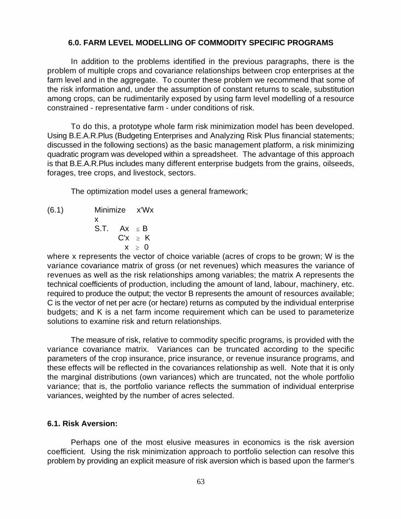
63

6.0. FARM LEVEL MODELLING OF COMMODITY SPECIFIC PROGRAMS

In addition to the problems identified in the previous paragraphs, there is theproblem of multiple crops and covariance relationships between crop enterprises at thefarm level and in the aggregate. To counter these problem we recommend that some ofthe risk information and, under the assumption of constant returns to scale, substitutionamong crops, can be rudimentarily exposed by using farm level modelling of a resourceconstrained - representative farm - under conditions of risk.

To do this, a prototype whole farm risk minimization model has been developed.Using B.E.A.R.Plus (Budgeting Enterprises and Analyzing Risk Plus financial statements;discussed in the following sections) as the basic management platform, a risk minimizingquadratic program was developed within a spreadsheet. The advantage of this approachis that B.E.A.R.Plus includes many different enterprise budgets from the grains, oilseeds,forages, tree crops, and livestock, sectors.

The optimization model uses a general framework;

(6.1) Minimize x'Wx x

S.T. Ax # B C'x $ K x $ 0where x represents the vector of choice variable (acres of crops to be grown; W is thevariance covariance matrix of gross (or net revenues) which measures the variance ofrevenues as well as the risk relationships among variables; the matrix A represents thetechnical coefficients of production, including the amount of land, labour, machinery, etc.required to produce the output; the vector B represents the amount of resources available;C is the vector of net per acre (or hectare) returns as computed by the individual enterprisebudgets; and K is a net farm income requirement which can be used to parameterizesolutions to examine risk and return relationships.

The measure of risk, relative to commodity specific programs, is provided with thevariance covariance matrix. Variances can be truncated according to the specificparameters of the crop insurance, price insurance, or revenue insurance programs, andthese effects will be reflected in the covariances relationship as well. Note that it is onlythe marginal distributions (own variances) which are truncated, not the whole portfoliovariance; that is, the portfolio variance reflects the summation of individual enterprisevariances, weighted by the number of acres selected.

6.1. Risk Aversion:

Perhaps one of the most elusive measures in economics is the risk aversioncoefficient. Using the risk minimization approach to portfolio selection can resolve thisproblem by providing an explicit measure of risk aversion which is based upon the farmer's

64

selection of a farm plan. This measure of risk aversion is obtained by taking the inverseon the shadow price or the income constraint (Turvey and Driver) and is an exact androbust measure. This measure can be obtained from the optimization model and used asa proxy within the general equilibrium model.

6.2. The B.E.A.R.Plus Farm Planning Program: A General Description

B.E.A.R.Plus is a farm management planning tool which operates in Quattro Proand provides a simple approach to farm management. It incorporates the key facets offarm financial planning, including enterprise budgets, financial statements and riskanalyses. There are three component to B.E.A.R.Plus, the Commander, the BudgetModule and the Financial Statements Module. The main purpose of the CommanderModule is to allow the user to move easily between the Budget and Financial StatementsModules.

6.2.1 The Budget Module - was developed to assist farmers in making management andplanning decisions. One of the most important and highly recommended practices is thedevelopment of enterprise budgets which are used to compare the profitability amongcompeting enterprises and in the context of the whole farm. Managers often budget thewhole farm in relation to outside competition, but place minor emphasis on competition forlimited resources within the farm. The Budget Module consolidates the enterprises (Crops,Livestock, fruits, and Vegetables) grown on the farm for comparison and evaluation.Included in B.E.A.R.Plus is over 60 enterprise budgets ranging from grain and oilseedcrops, to fruits, vegetables, beef, dairy, swine, poultry, sheep and goats. Budgets notincluded can be developed on request.

One of the unique and advanced features of B.E.A.R.Plus is its ability to performenterprise risk analyses. The inclusion of price and yield risk in the enterprise budgetsallows users to assess the probability that actual net enterprise revenues will fall aboveor below expected levels. Thus farmers, while hoping for favourable risk outcomes, cantake actions to ensure that fixed financial obligations and other cash flow requirements arefulfilled if an unfavourable risk outcome occurs.

6.2.2 The Financial Statements Module - is comprised of a set of coordinated farmfinancial statements including past and projected (cash and accrual) income statements,beginning and ending (historical cost or market value) balance sheets, statement ofchanges in financial position, statements of changes in owner's equity, debt-servicingcapacity report, a debt servicing worksheet, a cash flow statement and a farm businessanalysis report. If enterprise budgets are completed, data from the budgets can beimported to the financial statements module.

6.3. B.E.A.R.Plus and Whole Farm Optimization:

For purposes of this report, a quadratic programming module was added to

65

B.E.A.R.Plus, with the intent of providing a prototype model for investigating farm leveleffects of stabilization policies. The model queries the user for information regarding cropsgrown (through B.E.A.R.Plus), land available, resource utilization and machine timeavailable, labour requirements, and crop rotation practices. The user is also queried forup to 6 years of price and yield information as the basic input to risk analysis. Since rawdata is provided, this empirical distribution can be truncated, and by examining changesin expected values of prices, yields, and revenues, before and after truncation the actuarialvalue of crop insurance can be computed. Subsidies, measured by the difference betweenthe actuarial value of the stabilization policy, and the premium paid is then added to thegross margin of each enterprise considered. While only a few crops are examined in thisreal case farm study, the model can be used to analyze any combination of 8 crops, drawnfrom over 60 different enterprises. The model is not set up to examine NISA or other wholefarm stabilization policies, but the results of the optimization process can be used toevaluate these policies. In terms of the budget and financial statements module, only thebudgets module is used directly in the risk programming model, although information canbe transported to the financial statements module if required.

6.4. The Prototype Farm Planning Model:

This section provides the details of a spreadsheet modelling approach to evaluatingthe potential farm level impact of decoupled and partially decoupled agricultural policies.An actual case farm is then used to illustrate how the model can be used, and whatinformation can be obtained from it.

As argued in previous chapters much of the response to stabilization policies is dueto either risk reduction or income enhancement through subsidized premiums. The impactof stabilization policies on transfer efficiency is not direct because some of the benefits,e.g. risk reduction, can not ordinarily be measured in dollar terms. Subsidized premiums,on the other hand, can be measured directly, but the total effect of the subsidy should bemeasured in terms of the indirect output response as well as the direct income effect.

An appropriate methodology for measuring most of these effects is through farmlevel optimization and simulation. This research develops a prototype spreadsheetmodelling approach using the mathematical optimization routine in QUATTRO PRO anda Farm Planning Spreadsheet program called B.E.A.R.Plus (Budgeting Enterprises andAnalyzing Risks plus Financial Statements). The evaluation framework and methodologyis outlined in Figure 6.1.

The procedure starts with gathering information on a representative or case farm.The farm in this example is a 630 acre cash crop farm growing corn, white beans,soybeans, and wheat. Using enterprise budgets contained in B.E.A.R.Plus, gross marginsand anticipated yields were calculated. The example farmer maintained records andprovided 6 years of price and yield data. This data makes up the basic risk informationused in the analysis. The data are presented in Table 6.1.

66

Risk was measured in terms of truncated marginal probability distributions. Forexample if the policy being examined is crop insurance then the yield distribution wastruncated at the coverage level. The policies examined are crop insurance, crop plus priceinsurance, and gross revenue insurance.

67

Figure 6.1 the framework

68

Table 6.1 Historical Yields, Prices, and Revenues of Case Farm

Year 1993 1992 1991 1990 1989 1988 Avg. Std.

Crop Yield History (bu./acre, tonne/acre for whitebeans)

Corn 114 84 131 115 120 117 114 14.5

Beans 12 12 17 15 17 16 15 2.2

soy 39 31 54 42 32 34 39 7.9

Wheat 42 81 59 55 54 52 57 11.7

Crop Price History ($/bu., $/Tonne)

Corn 3.36 2.67 2.64 3.07 3.63 2.57 2.99 .40

Beans 23.90 20.30 22.80 25.58 32.54 21.99 24.52 3.94

Soy 7.93 6.18 6.26 6.61 8.46 7.19 7.11 .85

Wheat 2.80 3.21 3.16 3.81 4.16 4.62 3.63 .63

Crop Gross Revenue Histories ($/acre)

Corn 385 223 347 353 436 301 341 66.5

Beans 288 246 401 401 544 360 373 95.3

Soy 309 194 340 274 271 244 272 46.2

Wheat 119 259 188 210 225 240 207 45.2

69

Given the policy parameter, assumed for this example to be 85% coverage on alltypes of insurance, crop revenue variances and covariances were computed. These riskmeasures are used as the objective function in a risk minimizing quadratic program whichselects the most risk efficient farm plan given a specified level of expected income.Constraints on production are land, labour and machinery, with labour being hired asnecessary.

The comparative response to policies can be determined by optimizing the farmplan for each of the policies and comparing them to a no-policy run. The advantage of thisapproach is that different policies affect the risks of specific crops in different ways. Forexample, if a crop benefits more from crop insurance than price insurance, then ameasurable response can be obtained. In addition to this , since the measurement of risktakes into consideration the joint risks among crop substitution effects between crops canbe observed. For example if the benefits from insurance is greater for corn than soybeans,then a noticeable increase in acres of corn planted would be observed. The direct riskreducing benefits of agricultural policies can be evaluated by comparing the optimal farmplan of the policy without subsidized premiums, i.e. actuarially priced insurance, to the nopolicy scenario. The incremental effects of subsidized premiums can then be observed byrunning the model once again, with the incremental gains from insurance being includedin the marginal net revenues of the individual crops. This procedure is repeated for allpolicies to be examined.

Per acre risks are presented in Table 6.2 for the base case without insurance, andgross revenue insurance. In the base case the least risky crop is wheat, which isnegatively correlated with corn and soybeans. The most risky crop is white beans, followedby corn and soybeans. As expected in theory the highest risk crops also provide thehighest gross margin revenue. Gross margin revenues are $161/acre for corn, $220/acrefor white beans, $179/acre for soybeans, and $116/acre for wheat.

The second part of Table 6.2 illustrates the effect of stabilization policies on risk.The variance (measured in terms of $/acre squared) of corn for example is reduced from4,426 to 2,526, while the covariance between white beans and wheat is almost zero, at 11($/acre squared).

The actuarial price of the 3 insurance policies examined is found in Table 6.3. Thepremiums reflect the expected benefits from insurance and are measured on a $/acrebasis. For example, the highest price of crop insurance is for corn ($6.44/acre) while thelowest is for soybeans ($2.80/acre). A price coverage level of 85% is not sufficiently highto provide a benefit for corn and soybeans with price insurance, but price insurance isbeneficial to wheat. In terms of gross revenue insurance white beans has the highest cost.Corn premiums are zero, likely due to a strong negative correlation between prices andyields.

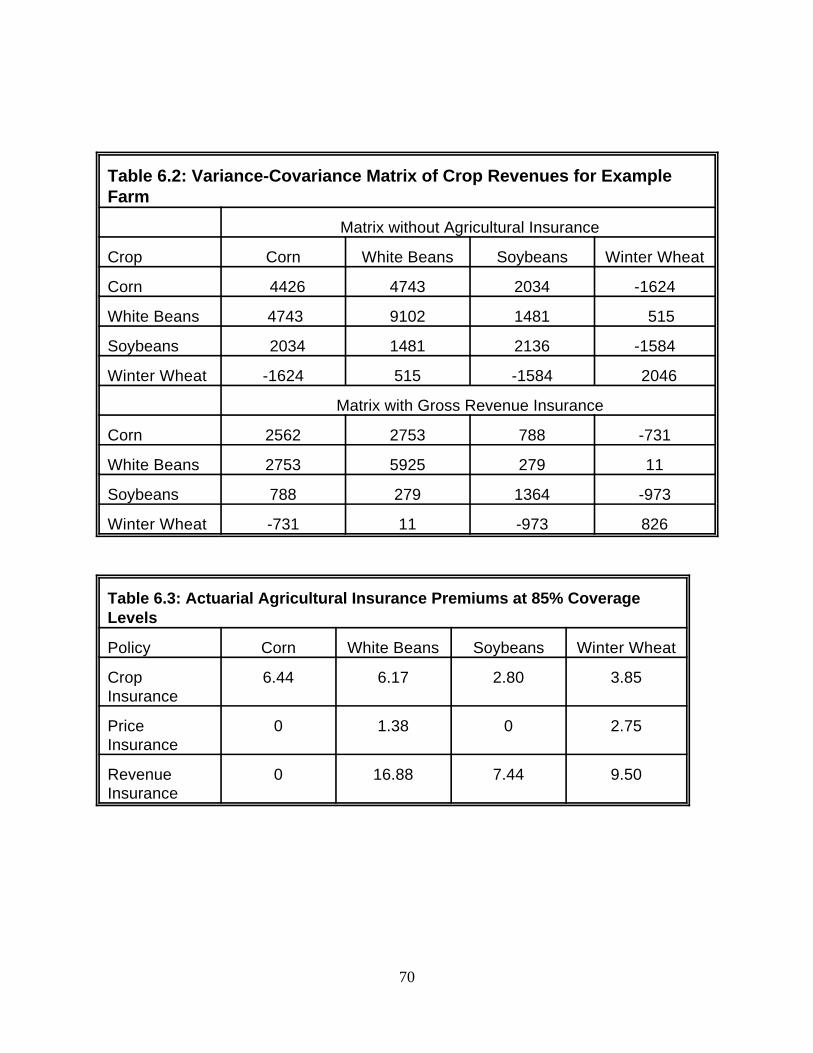
70

Table 6.2: Variance-Covariance Matrix of Crop Revenues for Example Farm

Matrix without Agricultural Insurance

Crop Corn White Beans Soybeans Winter Wheat

Corn 4426 4743 2034 -1624

White Beans 4743 9102 1481 515

Soybeans 2034 1481 2136 -1584

Winter Wheat -1624 515 -1584 2046

Matrix with Gross Revenue Insurance

Corn 2562 2753 788 -731

White Beans 2753 5925 279 11

Soybeans 788 279 1364 -973

Winter Wheat -731 11 -973 826

Table 6.3: Actuarial Agricultural Insurance Premiums at 85% CoverageLevels

Policy Corn White Beans Soybeans Winter Wheat

Crop 6.44 6.17 2.80 3.85Insurance

Price 0 1.38 0 2.75Insurance

Revenue 0 16.88 7.44 9.50Insurance

The risk aversion coefficient as measured depends on the portfolio selected. If a lower risk portfolio, with2

an expected return of $85,000 was selected this would imply a risk aversion coefficient of .0000977. In generalrisk aversion coefficients are going to reflect the income risk trade-offs, however they are also sensitive to scale.For use in the prototype D-T model the appropriate scale would depend upon the units of measurement. Forexample if dollar units were 1,000 times higher than those used here the same amount of risk aversion wouldbe of the order 98E-09. If profit maximization is assumed then the risk aversion coefficient would be 0.

71

Optimal farm plans are reported in Table 6.5, for all three policies. These solutionswill lie on an expected value=variance frontier such as that for the base case illustratedin Figure 6.2. In the absence of programs the farm would optimally grow 239 acres of corn,82 acres of white beans, 128 acres of soybeans, and 185 acres of wheat to obtainexpected income of $105,000 with a portfolio standard deviation of $23,620. By collectingthe inverse of the shadow price on the income constraint it is possible to obtain a riskaversion coefficient. The measured risk aversion of the case farmer is .0000147 which isappropriately scaled to income . The top scenario in Table 6.5 assumes that the farmer2

pays an actuarial price for protection so the only response is to reduced risk. There is noincome effect.

Under this assumption there are significant responses. For example, with cropinsurance alone, corn acres fall by 24% while soybean and white bean acres increase. Forcrop plus price insurance however there is no change in corn acres, and white beans fallby 24%. For Revenue insurance corn again falls by 24% and the response is similar to thecrop insurance case.

The income effect is noted in the lower part of Table 6.5. When insurance premiumsare subsidized this is viewed as a net increase in expected revenues. For crop insurancecorn acres increase by 1% which is in contrast to the 24% drop observed without hesubsidy. White beans which increased by 13% without the subsidy falls by 52% with the subsidy. Similarcontrasts are found for crop plus price insurance and revenue insurance.

It should be noted that all of the solutions in Table 6.5 have expected profits of$105,000. Hence farmers who target a particular income level for production can respondby reducing risk. Ideally, the quadratic program should maximize expected utility ratherthan minimize risk. One idea for this may be to run a farm plan using the risk minimizationmodel, and then derive from a given solution the risk aversion coefficient. Doing this wouldmake the income and risk reduction effects less transparent. The implication of the resultsare, however, clear. Stabilization policies do have an impact on farm portfolio decisionsand these impacts should be included in any measure of transfer efficiency at the farmlevel.

72

Figure 6.2 the E-V frontier

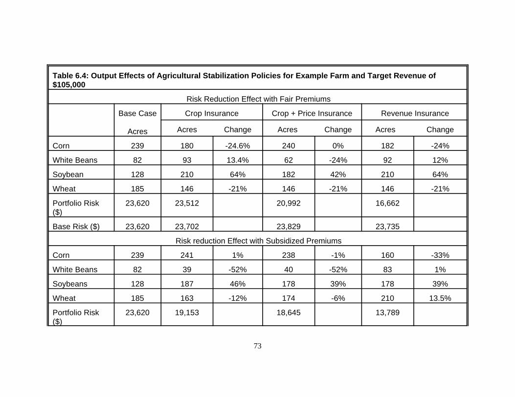
73

Table 6.4: Output Effects of Agricultural Stabilization Policies for Example Farm and Target Revenue of$105,000

Risk Reduction Effect with Fair Premiums

Base Case Crop Insurance Crop + Price Insurance Revenue Insurance

Acres Acres Change Acres Change Acres Change

Corn 239 180 -24.6% 240 0% 182 -24%

White Beans 82 93 13.4% 62 -24% 92 12%

Soybean 128 210 64% 182 42% 210 64%

Wheat 185 146 -21% 146 -21% 146 -21%

Portfolio Risk 23,620 23,512 20,992 16,662($)

Base Risk ($) 23,620 23,702 23,829 23,735

Risk reduction Effect with Subsidized Premiums

Corn 239 241 1% 238 -1% 160 -33%

White Beans 82 39 -52% 40 -52% 83 1%

Soybeans 128 187 46% 178 39% 178 39%

Wheat 185 163 -12% 174 -6% 210 13.5%

Portfolio Risk 23,620 19,153 18,645 13,789($)

74

Base Risk ($) 23.620 21,827 21,287 20,245

75

6.5. Potential Market Response to Agricultural Insurance:

In previous sections the impact of stabilization policies on supply and prices wasdiscussed. In Table 6.5 price flexibilities for the 4 crops are assumed to be -.1 for corn,soybeans and wheat, and because of the influence of Ontario white beans in the marketplace, -1 for white beans. Flexibilities can be used with a control optimization model if itassumed that technology at the farm level is linear homothetic which implies industryconstant returns to scale. Given this assumption the potential impact of the policies oncommodity prices can be derived. In the example the percentage change in prices is2.46% for unsubsidized crop insurance, but due to the smaller effect only a -.1% increasewhen the crop is subsidized. Stabilization policies favour other crops, mostly soybeans,over wheat in all but 1 instance. Market prices will increase modestly in all scenariosexcept subsidized revenue insurance which will decrease the price by 13.5%.

Table 6.5: Example of Price Flexibilities and Market Impact of Agricultural Insurance

Corn White Soybean WheatBeans

Price Flexibility (%change) -.1 -1 -.1 -.1

Crop No Subsidy 2.46% -13.4% -6.4% 2.1%

Insurance With Subsidy -.1% 52% -4.6% 1.2%

Crop + No Subsidy 0% 24% -4.2% 2.1%PriceInsurance With Subsidy -.1% 52% -3.9% .6%

Revenue No Subsidy -2.4% -12% -6.4% 2.1%

Insurance With Subsidy 3.3% -1% -3.9% -13.5%

6.6. Summary and Conclusion:

This chapter has outlined a methodology, developed a prototype model, illustratedhow agricultural policies affect farm level production decisions. It does not appear that anyof the commodity specific programs are decoupled. However, just because a program isnot decoupled does not necessarily mean that there will be an increased output response.Given limited resources, farmers will substitute the most favourable crops increasing

76

supply in some markets, but decreasing supply in others. The efficiency of agriculturalpolicies depends on the interrelationships among risky variables. In the above exampleeach crop was offered the same policy options, but still there were changes. However,there is a genuine ambiguity as to pure cause and effect, especially when it comes tosubstituting one source of risk for another.

Another issue relevant to the problem of transfer efficiency and discussed aboveis that not all policies are equal. Policy design can have an impact on the distribution ofresources within the farm, so that the true source of observed changes at the aggregatelevel cannot easily be distinguished. It is possible to examine these at the farm level usingsimple optimization models such as the one presented here.

Using a representative farm can also provide an indication of what the marketimpacts of a policy might be. In this chapter assumed price flexibilities were used toillustrate potential market price changes. While the changes appear to be dramatic insome instances, this is not unrealistic if in fact the relative shifts in product mix with therepresentative farm reflect typical farm decisions.

NISA/VAISA type programs were not included in this analysis because it wouldrequire a much more complex model requiring truncation of the joint probability distributionof outcomes as defined by the variance covariance matrix and the solutions. Furthermore,it is unlikely that NISA/VAISA type programs would have any real impact on risk bearing.For example, a risk response to VAISA (valued at gross margin such as is done here)would gain very little. In Figure 6.2 for example the farmer receiving $100,000 wouldcontribute perhaps $4000 into his NISA account. To increase this would require asubstantial increase in risk. For example, suppose that expected income were to increaseby $10,000. The incremental increase in NISA contributions would be only $400, yet theincrease in risk would be over $15,000. It is unlikely that farmers would be willing toincrease risk by so much for such modest gains in a risk free deposit account.

From another perspective, the base case scenario with $106,000 of income and aportfolio standard deviation $23,620 would only collect if (at 80% coverage) income fellbelow $84,800. The risk of the portfolio is such that the probability of exceeding $84,800is approximately 68%, which means that the chance of having to withdraw any amount isonly 32%. The fact that the likelihood of making a withdrawal is so much lower than thelikelihood of making a deposit adds further evidence to the contention that NISA-typeprograms are not going to induce dramatic increases in risk taking. Indeed, with the mostlikely outcome being deposits, these deposits take on significantly more importance andwould, then, be more likely encourage risk reducing behaviour, and portfolio shifts intolower risk, lower return crops.

77

REFERENCES

Alston, Julian M. and B. H. Hurd. 1990. Some Neglected Social costs of GovernmentSpending in Farm Programs. American Journal of Agricultural Economics, 33: 149-156.

Ballard, C. L. and D. Fullerton. 1992. Distortionary Taxes and the Provision of PublicGoods. Journal of Economic Perspectives, 6: 117-131.

de Gorter, H. and K. D. Meilke. 1989. Efficiency of Alternative Policies for the EC'sCommon Agricultural Policy. American Journal of Agricultural Economics, 71: 592-603.

Deloitte & Touche. 1993. How Governments Affect Agriculture? Report prepared forAgriculture Canada and the Industry Advisory Committee. Deloitte & ToucheManagement Consultants, 98 Macdonell Street, Guelph, Ontario.

Gardner, Bruce L. 1992. Changing Economic Perspectives on the Farm Problem. Journalof Economic Literature, 30: 62-101.

Gardner, Bruce L. 1987a. Causes of Farm Commodity Programs. Journal of PoliticalEconomy, 95: 290-310.

Gardner, Bruce L. 1987b. The Economics of Agricultural Policy. New York: MacmillanPublishing Company.

General Agreement on Tariff and Trade (GATT). 1994. Agreement on Agriculture.MTN/FA II-A1A-3, GATT, Geneva.

Just, R. E., D. L. Hueth and A. Schmitz. 1982. Applied Welfare Economics and PublicPolicy. New Jersey: Prentice Hall.

Magiera, S. L., N. Ballenger, M. E. Bredahl, R. House, K. Meilke, D. Orden and T. K.Warley. 1989. Report of the Task Force on The Reinstrumentation of AgriculturalPolicies. Working Paper # 89-7, International Agricultural Trade Research

Consortium.

Maier, L. 1994. The Costs and Benefits of U.S. Agricultural Policies with ImperfectCompetition in Food Manufacturing. New York: Garland Publishing.

McCalla, Alex F. and Harold O. Carter. 1976. Alternative Agricultural and Food PolicyDirections for the U.S. with Emphasis on a Market-Oriented Approach. In

Agricultural and Food Price and Income Policy, ed. Robert Spitze. AgriculturalExperiment Station, U. of Illinois Special Pub. 43, pp. 47-70.

78

McCalla, A. and T. Josling. 1985. Agricultural Policies and World Markets. New York:Macmillan.

Nerlove, Marc. 1958. The Dynamics of Supply. Baltimore: Johns Hopkins UniversityPress.

Rausser, Gordon C. and E. Hochman. 1979. Dynamic Agricultural Systems. New York:North Holland.

Stiglitz, J. E. 1987. Some Theoretical Aspects of Agricultural Policies. ResearchObserver, 2:43-60.

Turvey, C. G. and K. Chen. 1994. Canadian Safety Net Programs for Agriculture. Paperpresented at the AAEA Annual Meetings in San Diego, California.

Turvey, C.G. and Driver, H.C. 1986. Economics Analysis and Properties of the RiskAversion Coefficient in Constrained Mathematical Optimization. Canadian Journal ofAgricultural Economics. 34:125-137.

Tyrchniewicz, E. W. 1984. Western Grain Transportation Initiatives: Where Do We GoFrom Here? Canadian Journal of Agricultural Economics, 32: 253-268.

Wallace, T. D. 1962. Measures of Social Costs of Agricultural Programs. J. of FarmEconomics, 44: 580-594.

(A.1) EU(B) ' PY & C(Y) &82

Y 2F2p

(A.2) MEU(B)MY

' P & C )(Y) & 8YF2p ' 0 .

(A.3) P ' C )(Y) & 8YF2p

79

Appendix A: Risk Aversion and Production

This appendix develops the theoretical proposition underlying risk aversebehaviour, which states that producers, when faced with uncertain outcomes, will produceat below profit maximizing levels of output.

Here it is assumed that random price is described by P = )P + 0 where )P is thep

expected price and 0 a random deviate with mean equal to zero and variance F .p p2

A simple approach is to assume constant absolute risk aversion as the behaviourialconstraint. Then expected utility can be described by

where B is profits, Y is output, C(Y) is a quasi concave cost function, and 8 is thecoefficient of constant absolute risk aversion. Differentiating (A.1) with respect to outputyields,

The implicit solution to (A.2) provides the optimum level of output, Y . It is defined*

by

Under purely deterministic conditions or risk neutrality, )P = C'(Y), so the optimal level ofoutput is determined by setting expected prices equal to marginal costs.

The risk premium has a dampening effect on this condition. As Y increases so doesrisk and the risk premium (equal to 8/2 Y F in (A.1)). Risk averse producers will produce2 2

p

at an output level below the certainty level.

(B.1) V ' mPz

o(Pz&P)g(P)dP ' E 6Max [Pz&P,0]>

(B.2) V Y ' Y mPz

o(Pz&P) G(P)dP

(B.3) Y*V < Y mPz

o(Pz&P) G(P)dP

(B.4) (1&*)V Y1 .

80

Appendix B: Truncated Risk and the Pricing of Insurance

This appendix derives the mathematical relations of truncated distributions and thepricing of agricultural stabilization policies.

Mathematically, the formula for determining the actuarial value of agriculturalinsurance is given by;

In competitive insurance markets, V represents the actuarial value of insurance.In the absence of moral hazard and adverse selection, V plus a loading charge would bethe price that the farmer would pay for insurance coverage P . The term g(P) is thez

probability distribution function of P.

While the benefits of stabilization/insurance are paid on a unit price basis (e.g.bushels or tonnes) they are paid out on a long run average yield basis. Thus the truevalue of the program is equal to

where the left-hand side is the actuarial cost on a unit area basis (acre or hectare) and theright-hand side is the expected benefits.

There are two effects that price stabilization has on output decisions. The firsteffect deals with the subsidization of premiums while the second deals with the truncateddown-side risk.

If *, 0 # * < 1 is the rate of subsidization then

so that the expected net benefits are

(B.5) F2 ' mo(P&P)2 G(P)dP

(B.6) F2T ' m

P2

o(Pz&P)2 G(P)dP % mP2

(P&P)2 G(P)dP

' (Pz&P)2 G(Pz) % mPz(P&P)2 G(P)dP

(B.7) dF ' FT & F < 0 .

(B.8) FEU(B)MY

' P % (1&*)V & C )(Y) & 8Y F2T .

(B.9) P % (1&*)V ' C )(Y) % 8Y F2T .

81

The effect of stabilization/insurance on variance is to reduce downside risk. Bydefining variance as

The truncated variance is defined by

where G(P ) is the cumulative probability of price falling below P . The result is that thez z

change in variance due to insurance and stabilization is given by

This reduction in risk, combined with dP = (1-*) )YV (equation B.4) leads to the significantresponses to stabilization. To show this equation (A.3) can be modified as

The difference between equation (A.3) and equation (B.8) is the addition of (1-*) )YV asan increase marginal expected revenue and substituting F as the truncated variance.T

2

Rewriting yields the equilibrium condition

(C.1) Y ' Y % ,y

(C.2) EU(B) ' P Y & C(Y) &82

P 2 F2y .

(C.3) MEU(B)MY

' P & C )(Y) & 8 P 2 Fy

(C.4) P & C )(Y) ' 0

(C.5) Vy ' mYz

o(Yz&Y) F(Y)dY

(C.6) PVy ' PmYz

o(Yz&Y)F(Y)dY ,

82

Appendix C: Crop Insurance

To simplify the analytical approach it is assumed that prices are known and deterministicbut output are described by

where 0 is a random deviate from the mean )Y. The variance of yields is thus describedy

by F .y2

The expected utility model is defined by

Differentiating (C.2) with respect to Y gives

where MF /My indicates the change in risk with output. If increases in mean production arey2

variance preserving, then optimal output is given by the implicit solution to

and the optimum level of output will be higher.

The expected benefits of crop insurance are given by

which is usually on a yield per acre or hectare basis. Typically this is multiplied by anelected price so

(C.7) *yPVy < PmYz

o(Yz&Y) F(Y)dY .

(C.8) (1&*y) P MVy / MY

(C.9) MEU(B)MY

' P & C )(Y) % (1&*y) P MVy / MY & 8P 2 MFy / MY ' 0

83

and when subsidized by * ,y

Unlike price insurance a decision to increase output in response to the policy canincrease the premium as well. If (1-* ) )PV is the expected net income benefit fromy y

insurance then

indicates the change in the premium due to an output response, where MV /MY is positiveY

indicating that there is an interest to increase output based on the insurance subsidyalone. Substitution into the expected utility model's first order condition gives:

Here, as output increases and variance increases the expected benefits from subsidizationincrease. There is the potential for producers to balance the increased benefits frominsurance with the increased risk of increased production, in which case optimal outputwould occur at P = C'(Y) and production would appear as if the producer is risk neutral.If (1-* ) )PMV /MY > 8 MF /MY then output could actually increase to an amount greater thany y y

2

that implied by P = C'(Y).

(D.1) X ' X(P,W) ' X(W,Y(P,W))

(D.2) dX 'MXMW

dW %MXMY

MYMP

dP %MXMY

MYMW

dW

(D.3) dXdW

'MX(W,Y)

MW%

MX(W,Y)MY

MY(P,W)MW

# 0 ,

(D.4) dXdP

'MXMY

MYMP

$ 0

84

Appendix D: Impact of Stabilization on Input Demand and Input Markets

This section derives the mathematical relationships which show that increaseddemand for inputs can result from commodity specific programs if the programs are notoffered at an actuarial price.

If X refers to input demand then

refers to the demand as a function of input and output prices, and output.

Total differentiation yields,

and

and

If it is assumed that input prices do not adjust instantaneously to a price increase(i.e. perfectly elastic supply) then it can be assumed that the demand for inputs willincrease. In (25) dP refers to the increase in expected output price due to subsidizedagricultural insurance.