The Time Aspect of the Optimum Long-Term Open Pit Production Sequencing

2002 APCOM Symposium, Littleton, Colorado, USA

Copyright © 2002 SME

The Time Aspect of the Optimum Long-Term Open Pit

Production Sequencing*

Dr. Rossen Halatchev Private Consultant

Brisbane, AUSTRALIA

(*) This paper was published in the Proceedings of 2002 APCOM, p.133-146

ABSTRACT

The production sequence optimization of open pit mine is a procedure that reflects the exploitation conditions over life of mine. These conditions are determined by the geological characteristics of the deposit, requirements of the mining and processing technologies and economic parameters of the exploitation. From a technological point of view the production sequence optimization deals with two aspects – spatial and time. Each of them plays a tremendously important role in searching for the optimum solution of the problem. This paper treats the time aspect of the production sequence optimization. This aspect is revealed in the context of the problem of the working zone formation of the open pit mine in time. The problem formulation places an accent on the determination of the theoretically possible time distribution of the waste and ore quantities of each bench of the open pit mine. A mathematical solution to the problem has been developed based on combinatorial analysis. The solution provides a multi-variant investigation of the production sequencing with the use of an optimization model developed as a linear programming formulation. The model objective function uses the Net Present Value as a criterion for assessing the effectiveness of production sequencing. A case study is provided for the conditions of Assarel copper open pit mine (Bulgaria) to illustrate the applicability of the approach. The results obtained reveal the complex nature of the variation of the Net Present Value as a function of the mining factor.

INTRODUCTION

The problem of production sequencing optimization is a key problem in the contemporary theory of surface mining. Its solution deals directly with the management of the cash flows of each mining venture as production sequencing is considered as a first phase of the procedure of production scheduling. In other words production sequencing optimization provides the starting point of production scheduling optimization. The importance of the problem of production sequencing optimization is due to a large extent to the fact that its solution is sought always in the context of the determination of the mining system of the open pit mine exploitation over life of mine. Any mining system currently known deals with the order and direction of conducting the mining operations within the space enclosed within the ultimate pit outlines. On the other hand the production sequencing optimization also deals with the determination of the time of inclusion of the cutbacks in the mine exploitation under the requirement for meeting the mill ore demand. Another aspect of the problem importance is that the optimal production sequence of the mine, in principle, is used as a base for implementing a cutoff grade strategy in the context of the recent developments in this particular field [Lane, 1988]. In this way the optimality of the cutoff grade solution can be achieved only in an interactive way with regard to the optimality of the production sequence solution.



The problem of production sequencing has found a place in the investigations of many researchers. Significant achievements in this direction have been reached by Tan & Ramani [1992], Onur & Dowd [1993], Kim & Zhao [1994], Sevim & Lei [1996], Wang [1996], Akaike & Dagdelen [1999], Hoerger, Bachmann, Criss & Shortridge [1999]. These achievements constitute the framework for a rational approach to the problem of production sequencing optimization. The present paper offers a new vision for the problem, which places a strong emphasis on the time aspect of the production sequencing optimization and the implementation of the principle of waste deferment as one of the basic principles of mine planning.

PROBLEM FORMULATION

Production sequencing, from a technological point of view, has two aspects of consideration – spatial and time. The spatial aspect deals with the determination of the shape and size of the pit benches. In the theory of surface mining this is known as a geometric sequencing [Hustrulid & Kuhta, 1995]. The geometrical sequencing usually is achieved with the discretization of the pit space within the ultimate pit outlines into pit units. There are two known approaches for generating pit units. The first approach uses an economic discretization, which leads to designing the so-called cut-backs or push-backs, which have variable working widths. The approach is widely spread in the mining practice and it implements dominantly the famous method of Lerchs-Grossmann for generating pit shells. The other approach uses a technological discretization of the pit space into pit units, where the minimum working width is the limiting technological factor. The working widths of the benches are relatively constant and they are determined as a function of the size of the production equipment as well as the technological scheme for conducting the mining operations in the faces of the benches. The time aspect of production sequencing treats the formation of the mine production sequence in time. This formation refers to the meaning of arranging the bench rock quantities as a flow of the pit supply. This formation also means a determination of the working zone of the open pit mine, which can cover the mining operations conducted simultaneously on the benches of many pit units. For example, the production sequence of the mine can be presented as a summation of the sequences of a few cut-backs. The formulation of the problem for determining the theoretically possible variants of the mine production sequence arrangement in time is based on the following assumptions: � the sequence of each cutback is formed in the scheme “bench after bench” of conducting the

mining operations down to the bottom; � the total length of each bench (Lb) coincides with the length of the shovel front (Lb): Lb = Lsf,

i.e. each bench is excavated only by one shovel. In principle, there are other technological schemes that meet the condition Lb > Lsf;

� the mine sequence is presented by 3 possible rock types: waste, basic ore type and secondary ore. The basic ore type has a grade higher or equal to the mill-feed cutoff grade and it feeds the mill. The grade of secondary ore type is between the mill-feed cutoff grade and break-even cutoff grade. This ore type has a potential economic value and goes to stockpiles for future treatment;

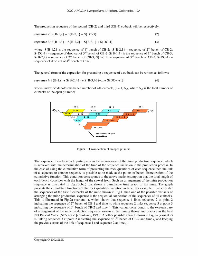
� The problem solution meets the objectives of long-term planning. Based on these assumptions let’s consider a cross-section of an example open pit mine shown in Fig.1. The pit space is discretized into cutbacks. The production sequence of the first cutback (CB-1) can be presented conditionally as follows:

sequence 1: S{B-1,1} + S{DC-2} (1) where: S{B-1,1} is the sequence of 1st bench of CB-1; S{DC-2} – sequence of drop cut of 2nd bench of CB-2;



The production sequence of the second (CB-2) and third (CB-3) cutback will be respectively: sequence 2: S{B-1,2} + S{B-2,1} + S{DC-3} (2) sequence 3: S{B-1,3} + S{B-2,2} + S{B-3,1} + S{DC-4} (3) where: S{B-1,2} is the sequence of 1st bench of CB-2; S{B-2,1} – sequence of 2nd bench of CB-2; S{DC-3} – sequence of drop cut of 3rd bench of CB-2; S{B-1,3} is the sequence of 1st bench of CB-3; S{B-2,2} – sequence of 2nd bench of CB-3; S{B-3,1} – sequence of 3rd bench of CB-3; S{DC-4} – sequence of drop cut of 4th bench of CB-3; The general form of the expression for presenting a sequence of a cutback can be written as follows: sequence i: S{B-1,i} + S{B-2,i-2} + S{B-3,i-3}+…+ S{DC-(i+1)} (4) where: index “i” denotes the bench number of i-th cutback, (i = 1, Ncb, where Ncb is the total number of cutbacks of the open pit mine).

Figure 1. Cross-section of an open pit mine

The sequence of each cutback participates in the arrangement of the mine production sequence, which is achieved with the determination of the time of the sequence inclusion in the production process. In the case of using the cumulative form of presenting the rock quantities of each sequence then the link of a sequence to another sequence is possible to be made at the points of bench discretization of the cumulative function. This condition corresponds to the above-made assumption that the total length of each bench coincides with the length of the shovel front. Such an arrangement of the mine production sequence is illustrated in Fig.2(a,b,c) that shows a cumulative time graph of the mine. The graph presents the cumulative functions of the rock quantities variation in time. For example, if we consider the sequences of the first 3 cutbacks of the mine shown in Fig.1, then one of the possible variants of arranging the mine production sequence is the sequential connection of the sequences of all cutbacks. This is illustrated in Fig.2a (variant 1), which shows that sequence 1 links sequence 2 at point 2 indicating the sequence of 2nd bench of CB-1 and time t1, while sequence 2 links sequence 3 at point 3 indicating the sequence of 3rd bench of CB-2 and time t2. This variant corresponds to the extreme case of arrangement of the mine production sequence known in the mining theory and practice as the best Net Present Value (NPV) case [Halatchev, 1993]. Another possible variant shown in Fig.2a (variant 2) is linking sequence 3 at point 2 indicating the sequence of 2nd bench of CB-2 and time t2 and keeping the previous status of the link of sequence 1 and sequence 2 at time t1.



Figure 2a. Cumulative time graph of the mine: variant 1 & variant 2

Figure 2b. Cumulative time graph of the mine: variant 3 & variant 4

Figure 2b shows two other theoretically possible variants of arrangement of the mine production sequence (variant 3 and variant 4) in the cumulative time graph. Variant 3 links sequence 3 at point 1 indicating the sequence of 1st bench of CB-2 and time t2 and keeping the previous status of the link of sequence 1 and sequence 2 at time t1. Variants 4 links sequence 2 at point 1 indicating the sequence of 1st bench of CB-1 and time t1 and keeping the status of sequential connection of sequence 2 and sequence 3 at time t2.

Figure 2c. Cumulative time graph of the mine: variant 5 & variant 6

There are another 2 possible variants (variant 5 and variant 6) shown in Fig.2c. Variant 5 links sequence 2 at point 1 indicating the sequence of 1st bench of CB-1 and time t1. Sequence 3 is linked at point 2 indicating 2nd bench of CB-2 and time t2. Variant 6 is the last theoretically possible variant. It shows that sequence 2 is linked at point 1 indicating the sequence of 1st bench of CB-1 and time t1



while sequence 3 is linked at point 2 indicating 1st bench of CB-2 and time t2. This variant is very close by technological content to the other extreme case of arrangement of the mine production sequence known as the worst NPV case [Halatchev, 1993]. The variants described give ground to conclude that the solution of the problem for determining the theoretically possible time distribution of the waste and ore quantities of each cutback bench has a multi-variant character. The two variants that correspond to the extreme best and worst NPV cases of the production sequence arrangement determine the limits of the range of all possible theoretical variants of the problem solution. The determination of the number of theoretically possible variants (

totalN ) of arranging the mine production sequence as a function of the sequences of all cutbacks of the

mine can be done with the following formula:

∏−

=

=1N

1k

ktotal

cb

mN (5)

where: mk is the number of benches of k-th cutback. Each variant of the mine production sequence arrangement, indeed, represents a variant of the formation of the working zone of the open pit mine. In this way formula (5) determines the theoretically possible variants of the formation of the working zone of the mine over life of mine.

METHOD OF PRODUCTION SCHEDULING OPTIMIZATION

The assessment of the economic effectiveness of the mine production sequencing is possible to be done only through the assessment of the production scheduling effectiveness. This specific feature explains the difference in principle between both technological procedures. The procedure of the mine production sequencing with regard to the time aspect deals only with the order of inclusion of the sequences of the cutbacks in the production process. The procedure of the production scheduling, on the other hand, deals with the transformation of the mine production sequence into a schedule that meets certain technological requirements. For example, such a requirement can be the implementation of a schedule with a constant mining rate or a schedule with a multi-stage stabilization of the mining rate. That is why the production scheduling possesses the property to assess the real economy of the mine exploitation as it determines the quantity and quality of the mining production. The method, which can implement the technique described above for determining the theoretically possible variants of the mine production sequence arrangement in time, uses the cumulative spatial and time graphs of the open pit mine as a basis of the production scheduling optimization procedure [Halatchev, 1993; Halatchev & Moustakerov, 1996]. Both graphs have a direct link as the cumulative function of the rock quantities in the cumulative time graph is presented as a mine production sequence corresponding to the curve of the best NPV case of the cumulative spatial graph. So, the cumulative function in question is defined as a common upper bound function of the rock quantities of the best NPV case. The optimum production sequence usually differs from the production sequence of the best NPV case, which is due to the conflict character of the variables participating in the optimization model of production scheduling developed as a linear programming formulation. The objective function of the optimization scheduling model has the following expression [Halatchev, 1993]:

+−−−+∑=

−

iiiiiii b

n

0i

p

b

m

bb

s

bbb

i PCCCSr1MAX )()( γγ

+−−−++ ∑=

−

iiiiiii s

n

0i

p

s

m

ss

s

sss

i PCCCSr1 )()( γγ



+ ∑∑∑∑∑= =

−

= =

−

=

− +−+−+m

1k

n

oi

kiki

im

1k

n

oi

kiki

i

i

n

0i

w

iDCur1NChr1VCr1

i)()()( (6)

where: r is the discount rate; ii sb SS , – price of basic ore type (BOT) and secondary ore type (SOT)

metal; s

s

s

b iiCC , - unit marketing cost of BOT and SOT metal;

m

s

m

b i1CC , - unit operating cost of BOT and

SOT mining; p

s

p

b iiCC , - unit operating cost of BOT and SOT processing;

iwC – unit operating cost of

waste removal; hki – unit purchase cost of production capacity of k-th shovel model; uki – unit

ownership cost of production capacity of k-th shovel model; ii sb PP , -production of BOT and SOT; Vi –

waste removal; NCki – increase of equipment capacity of k-th shovel model; DCki – decrease of equipment capacity of k-th shovel model, m – number of shovel models; n – number of time periods over life of mine. The index “i” in the objective function (6) denotes i-th time period of production scheduling optimization over life of mine. The last two terms of the objective function manage the location of the optimum production sequence in the feasible domain of the cumulative spatial graph, which results in a schedule type of multi-stage stabilization of the mining rate. CASE STUDY

Object of investigation: The case study deals with the Assarel copper open pit mine (Bulgaria). It is organized with regard to 4 cutbacks of the mine in order to show the applicability of the method for modelling all theoretically possible variants of the time arrangement of the mine production sequence. The technological ore flow of the mine is divided into two types – basic ore type (BOT) and secondary ore type (SOT). The BOT goes directly to the processing plant for producing floatation concentrate, while the SOT is stockpiled for a succeeding leaching and production of a cement concentrate. Computer implementation: The computer code “ANGEL” was developed in QuickBasic and used for the case study. The code initially calculates the input data of the production scheduling optimization and then it calls the LINDO solver – student version [Winston, 1994] as an external code for running the optimization model of production scheduling. Input data: copper price – 1800$/t; unit operating cost of BOT and SOT mining – 1.2$/t; unit operating cost of BOT processing - 3.6$/t; unit operating cost of SOT processing – 1.6$/t; unit operating cost of waste removal – 1.65$/t; interest rate – 10%. The data is borrowed from [Halatchev, 1999]. The data of the unit purchase and ownership costs of production capacity of each shovel model are summarized in Table 1. The cutoff grade is accepted to be a constant quantity over life of mine.

Table 1. Data of shovel models used

Shovel model

Number of shovels

Unit purchase cost of production capacity

$/t

Unit ownership cost of production capacity

$/t

Liebherr 994 2 0.3786 0.2272 Dresser 580 1 0.3855 0.2313

EKG_8I 2 0.3161 0.1897 EKG_4I 2 0.3331 0.1999

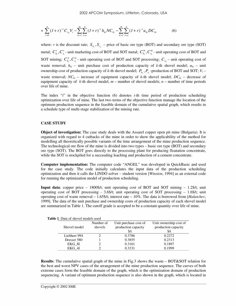
Results: The cumulative spatial graph of the mine in Fig.3 shows the waste – BOT&SOT relation for the best and worst NPV cases of the arrangement of the mine production sequence. The curves of both extreme cases form the feasible domain of the graph, which is the optimization domain of production sequencing. A variant of optimum production sequence is also shown in the graph, which is located in



the feasible domain. The optimum production sequence is a result of the implementation of the production scheduling optimization model described above and it can be treated as the optimum NPV case.

Figure 3. Cumulative spatial graph of Assarel copper mine

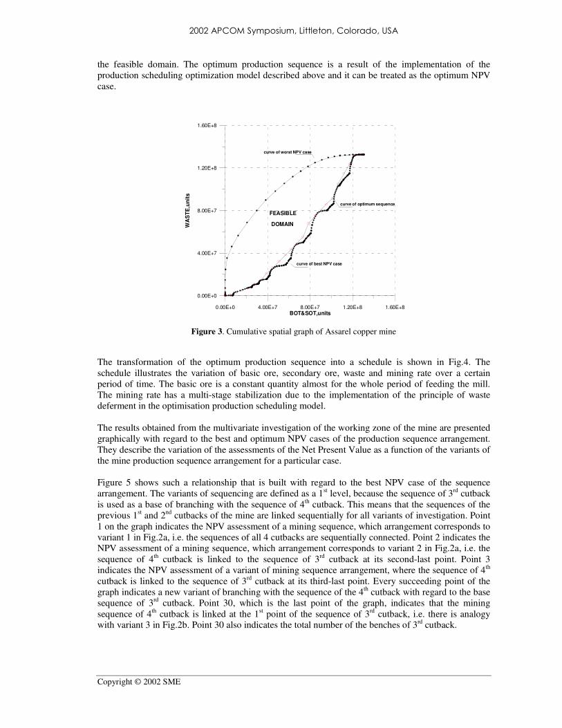
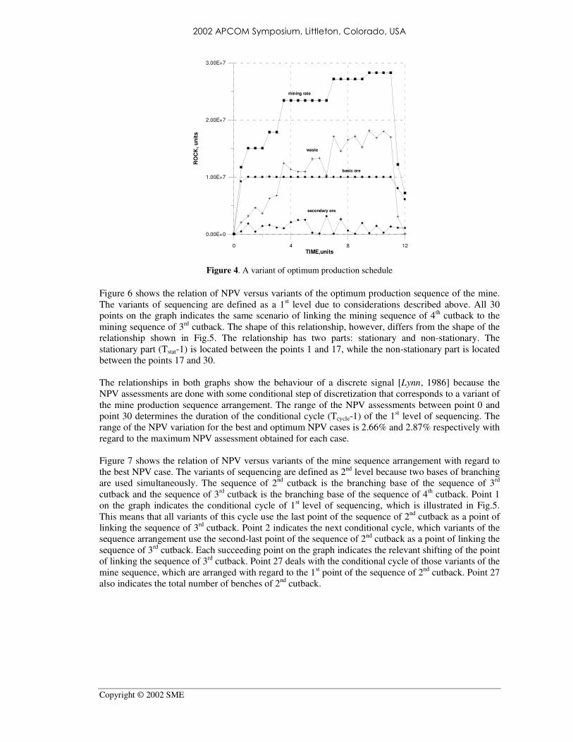
The transformation of the optimum production sequence into a schedule is shown in Fig.4. The schedule illustrates the variation of basic ore, secondary ore, waste and mining rate over a certain period of time. The basic ore is a constant quantity almost for the whole period of feeding the mill. The mining rate has a multi-stage stabilization due to the implementation of the principle of waste deferment in the optimisation production scheduling model. The results obtained from the multivariate investigation of the working zone of the mine are presented graphically with regard to the best and optimum NPV cases of the production sequence arrangement. They describe the variation of the assessments of the Net Present Value as a function of the variants of the mine production sequence arrangement for a particular case. Figure 5 shows such a relationship that is built with regard to the best NPV case of the sequence arrangement. The variants of sequencing are defined as a 1st level, because the sequence of 3rd cutback is used as a base of branching with the sequence of 4th cutback. This means that the sequences of the previous 1st and 2nd cutbacks of the mine are linked sequentially for all variants of investigation. Point 1 on the graph indicates the NPV assessment of a mining sequence, which arrangement corresponds to variant 1 in Fig.2a, i.e. the sequences of all 4 cutbacks are sequentially connected. Point 2 indicates the NPV assessment of a mining sequence, which arrangement corresponds to variant 2 in Fig.2a, i.e. the sequence of 4th cutback is linked to the sequence of 3rd cutback at its second-last point. Point 3 indicates the NPV assessment of a variant of mining sequence arrangement, where the sequence of 4th cutback is linked to the sequence of 3rd cutback at its third-last point. Every succeeding point of the graph indicates a new variant of branching with the sequence of the 4th cutback with regard to the base sequence of 3rd cutback. Point 30, which is the last point of the graph, indicates that the mining sequence of 4th cutback is linked at the 1st point of the sequence of 3rd cutback, i.e. there is analogy with variant 3 in Fig.2b. Point 30 also indicates the total number of the benches of 3rd cutback.

0.00E+0 4.00E+7 8.00E+7 1.20E+8 1.60E+8

BOT&SOT,units

0.00E+0

4.00E+7

8.00E+7

1.20E+8

1.60E+8

WA

ST

E,u

nit

s

curve of best NPV case

curve of worst NPV case

curve of optimum sequence

FEASIBLE

DOMAIN



Figure 4. A variant of optimum production schedule

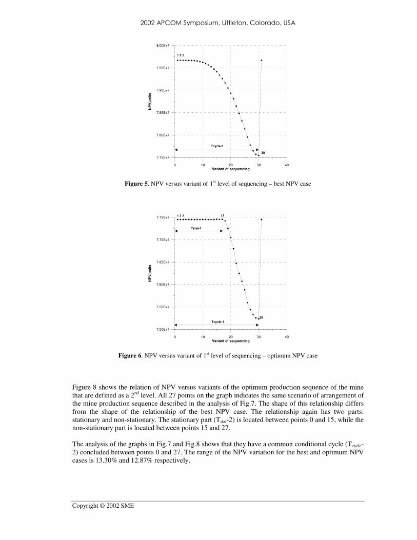
Figure 6 shows the relation of NPV versus variants of the optimum production sequence of the mine. The variants of sequencing are defined as a 1st level due to considerations described above. All 30 points on the graph indicates the same scenario of linking the mining sequence of 4th cutback to the mining sequence of 3rd cutback. The shape of this relationship, however, differs from the shape of the relationship shown in Fig.5. The relationship has two parts: stationary and non-stationary. The stationary part (Tstat-1) is located between the points 1 and 17, while the non-stationary part is located between the points 17 and 30. The relationships in both graphs show the behaviour of a discrete signal [Lynn, 1986] because the NPV assessments are done with some conditional step of discretization that corresponds to a variant of the mine production sequence arrangement. The range of the NPV assessments between point 0 and point 30 determines the duration of the conditional cycle (Tcycle-1) of the 1st level of sequencing. The range of the NPV variation for the best and optimum NPV cases is 2.66% and 2.87% respectively with regard to the maximum NPV assessment obtained for each case. Figure 7 shows the relation of NPV versus variants of the mine sequence arrangement with regard to the best NPV case. The variants of sequencing are defined as 2nd level because two bases of branching are used simultaneously. The sequence of 2nd cutback is the branching base of the sequence of 3rd cutback and the sequence of 3rd cutback is the branching base of the sequence of 4th cutback. Point 1 on the graph indicates the conditional cycle of 1st level of sequencing, which is illustrated in Fig.5. This means that all variants of this cycle use the last point of the sequence of 2nd cutback as a point of linking the sequence of 3rd cutback. Point 2 indicates the next conditional cycle, which variants of the sequence arrangement use the second-last point of the sequence of 2nd cutback as a point of linking the sequence of 3rd cutback. Each succeeding point on the graph indicates the relevant shifting of the point of linking the sequence of 3rd cutback. Point 27 deals with the conditional cycle of those variants of the mine sequence, which are arranged with regard to the 1st point of the sequence of 2nd cutback. Point 27 also indicates the total number of benches of 2nd cutback.

0 4 8 12

TIME,units

0.00E+0

1.00E+7

2.00E+7

3.00E+7

RO

CK

, u

nit

s

mining rate

waste

basic ore

secondary ore



Figure 5. NPV versus variant of 1st level of sequencing – best NPV case

Figure 6. NPV versus variant of 1st level of sequencing – optimum NPV case

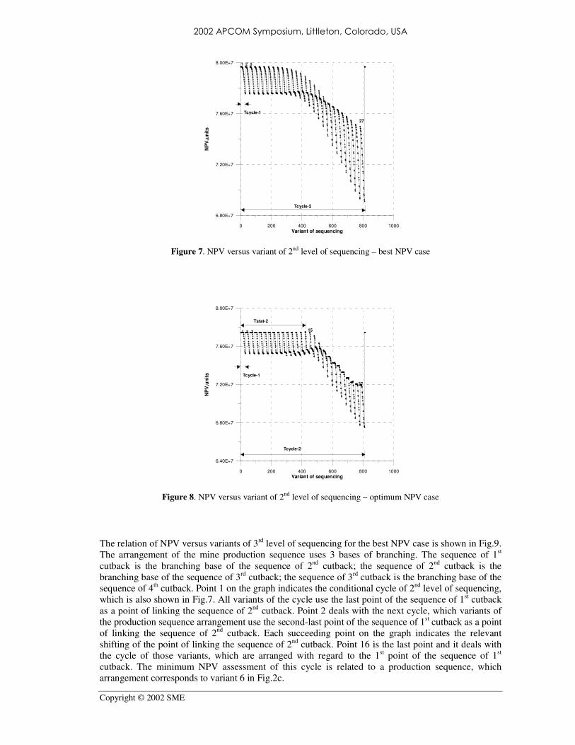
Figure 8 shows the relation of NPV versus variants of the optimum production sequence of the mine that are defined as a 2nd level. All 27 points on the graph indicates the same scenario of arrangement of the mine production sequence described in the analysis of Fig.7. The shape of this relationship differs from the shape of the relationship of the best NPV case. The relationship again has two parts: stationary and non-stationary. The stationary part (Tstat-2) is located between points 0 and 15, while the non-stationary part is located between points 15 and 27. The analysis of the graphs in Fig.7 and Fig.8 shows that they have a common conditional cycle (Tcycle-2) concluded between points 0 and 27. The range of the NPV variation for the best and optimum NPV cases is 13.30% and 12.87% respectively.

0 10 20 30 40

Variant of sequencing

7.75E+7

7.80E+7

7.85E+7

7.90E+7

7.95E+7

8.00E+7

NP

V,u

nit

sTcycle-1

30

0 10 20 30 40


7.50E+7

7.55E+7

7.60E+7

7.65E+7

7.70E+7

7.75E+7

NP

V,u

nit

s

Tcycle-1

Tstat-1

30

17



Figure 7. NPV versus variant of 2nd level of sequencing – best NPV case

Figure 8. NPV versus variant of 2nd level of sequencing – optimum NPV case

The relation of NPV versus variants of 3rd level of sequencing for the best NPV case is shown in Fig.9. The arrangement of the mine production sequence uses 3 bases of branching. The sequence of 1st cutback is the branching base of the sequence of 2nd cutback; the sequence of 2nd cutback is the branching base of the sequence of 3rd cutback; the sequence of 3rd cutback is the branching base of the sequence of 4th cutback. Point 1 on the graph indicates the conditional cycle of 2nd level of sequencing, which is also shown in Fig.7. All variants of the cycle use the last point of the sequence of 1st cutback as a point of linking the sequence of 2nd cutback. Point 2 deals with the next cycle, which variants of the production sequence arrangement use the second-last point of the sequence of 1st cutback as a point of linking the sequence of 2nd cutback. Each succeeding point on the graph indicates the relevant shifting of the point of linking the sequence of 2nd cutback. Point 16 is the last point and it deals with the cycle of those variants, which are arranged with regard to the 1st point of the sequence of 1st cutback. The minimum NPV assessment of this cycle is related to a production sequence, which arrangement corresponds to variant 6 in Fig.2c.

0 200 400 600 800 1000


6.80E+7

7.20E+7

7.60E+7

8.00E+7

NP

V,u

nit

sTcycle-2

Tcycle-1

27

0 200 400 600 800 1000


6.40E+7

6.80E+7

7.20E+7

7.60E+7

8.00E+7

NP

V,u

nit

s

Tcycle-2

Tcycle-1

Tstat-2

15

27



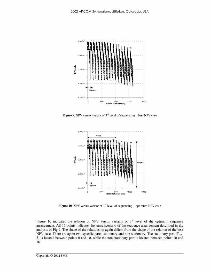
Figure 9. NPV versus variant of 3rd level of sequencing – best NPV case

Figure 10. NPV versus variant of 3rd level of sequencing – optimum NPV case

Figure 10 indicates the relation of NPV versus variants of 3rd level of the optimum sequence arrangement. All 16 points indicates the same scenario of the sequence arrangement described in the analysis of Fig.9. The shape of the relationship again differs from the shape of the relation of the best NPV case. There are again two specific parts: stationary and non-stationary. The stationary part (Tstat-3) is located between points 0 and 10, while the non-stationary part is located between points 10 and 16.

0 4000 8000 12000 16000


6.40E+7

6.80E+7

7.20E+7

7.60E+7

8.00E+7

NP

V,u

nit

s

Tcycle-2

1 2 3

16

0 4000 8000 12000 16000

Varianrt of sequencing

6.40E+7

6.80E+7

7.20E+7

7.60E+7

8.00E+7

NP

V,u

nit

s

Tcycle-2

Tstat-3

Range-3

10

16



The range of the NPV variation for the best and optimum NPV cases is 13.27% and 15.84% respectively. These assessments of the range of the NPV variation, indeed, are the overall assessments of the present case study. They reveal the economic potential of the mine exploitation in terms of all theoretically possible variants of modelling its working zone.

The analysis of the results obtained for all levels of sequencing for the best NPV case shows that there is a common trend in decreasing the NPV assessments for each succeeding cycle. This can be explained with the fact that each succeeding cycle indicates an earlier inclusion of some waste quantity in the mine exploitation, which leads to increasing the operating costs of waste removal. As a result of that the NPV assessment is affected by the implementation of the discount rate, which accounts the time effect of money. All relationships that deal with the optimum NPV case (Fig.6, 8, 10) are characterized with two parts: stationary and non-stationary. Obviously this specific feature is determined by the feasible domain of the cumulative spatial graph, which is used as an optimization domain of the production sequence optimization. Hence, the feasible domain possesses the property to produce a stationary part of the relation of NPV versus variant of optimum production sequence for each level of production sequencing. The non-stationary parts have the same explanation, which is provided above for the best NPV case of the production sequence arrangement (Fig.5, 7, 9). The NPV assessments that are related to the stationary part of the 1st level of sequencing for the optimum NPV case determine the maximum assessments of NPV variation for all succeeding levels of sequencing. It is worth noting that the relationships in Fig.6, 8 and 10 have a purely theoretical meaning because all variants of optimization of production sequence are not checked with regard to the technological requirement about the dynamics of the mining operations. This requirement aims to exclude any geometrical incompatibility of the formation of the working zone of the mine at the simultaneous exploitation of two and more cutbacks [Halatchev, 1993]. The relationships in Fig.6, 8 and 10 also can not give an answer to the question about the optimal production sequence among all optimum production sequences of the present multi-variant investigation. Every optimum production sequence implements to some degree the principle of waste deferment, which produces a schedule with a certain mining rate variation. This specific feature of the optimization of production sequence raises the matter for implementing another additional criterion to the decision-making process. Such a criterion has to deal with the viability of the mining project with regard to the choice of a practical schedule. Hence, the problem of searching for the optimal production sequence can be solved only with the implementation of multi-criteria formulation of production scheduling optimization, which has to account compulsory for the dynamics of the mining operations and viability of the production schedules. CONCLUSIONS

The technique presented in the paper provides a solution of the complex problem for modelling all theoretically possible variants of the formation of the working zone of an open pit mine through the investigation of the time aspect of production sequencing. It uses a combinatorial analysis, which simplifies the research approach. The results obtained from the technique implementation for the conditions of Assarel copper open pit mine shows that the theoretical relation of NPV versus variants of optimum production sequence arrangement reveals a large economic potential of the current mine exploitation, which is within 15.84% of the NPV variation for the scenario of cutback arrangement used in the present case study. This economic potential can be used as a reserve against the price volatility. The problem of determining the optimal production sequence among all theoretically possible variants of optimum production sequence requires further investigations about the viability of the optimum production schedules, which will determine the optimum limits of the implementation of the principle of waste deferment.



The general conclusion that can be drawn from the results of the present case study is that the mining factor plays as important a role for any surface mining venture as the other two basic factors, geological and economic. ACKNOWLEDGEMENT

The author of the present paper wishes to thank all colleagues who helped him directly or indirectly in his long-term research attempts to develop a new methodology of production scheduling. The results presented in the paper mark a certain stage of the methodology development. All comments about the paper can be sent to the address: [email protected].

REFERENCES Akaike, A. and K. Dagdelen, 1999. A strategic production scheduling method for an open pit mine. Proceedings

APCOM-99, October 20-22, 1999, Colorado School of Mines, Golden, Colorado, pp.729-738. Halatchev, R., 1993. Stage opencut exploitation of ore deposit. Proceedings 1993 Conference on the

Applications of Computers in the Mineral Industry, 5-7October, 1993, Wollongong, pp. 320-327. Halatchev, R. and I. Moustakerov, 1996. Optimum scheduling of waste and ore production. Mining Technology

Journal, Febr., Vol. 78, No. 894, pp. 61-64. Halatchev, R., 1999. Company strategy – a basis for production scheduling of an open pit complex. Proceedings

Strategic Mine Planning Conference, 23-24 March, 1999, Perth, pp.81-96. Hoerger, S., J. Bachmann, K. Criss and E. Shortridge, 1999. Long term mine and processing scheduling at

Newmont’s Nevada Operations. Proceedings APCOM-99, October 20-22, 1999, Colorado School of Mines, Golden, Colorado, pp.739-748.

Hustrulid, W. and M. Kuhta, 1995. Open pit mine planning and design. Balkema: Rotherdam, p.633. Kim, C. and Y. Zhao, 1994. Optimum open pit production sequencing – the current state of the art, in

Proceedings SME Annual Meeting 1994, Preprint N-94-224 (SME: Littleton). Lane, K., 1988. The economic definition of ore – cut-off grades theory and practice. London: Mining Journal

Books Ltd., p.149. Lynn, A., 1986. Electronic signals and systems. Macmillian Education Ltd: London, p.332. Onur, A. and P. Dowd, 1993. Open-pit optimization – part 2: production scheduling and inclusion of roadways.

Trans. Instn. Min. Metall. (Sect. A: Min. Industry), 102, pp. A105-A113. Sevim, H. and D. Lei, 1996. Production planning with working-slope maximum-metal pit sequences, Trans.

Instn Min. Metall.(Sect. A: Mining Industry), 105, pp.A93-98. Tan, S. and R. Ramani, 1992. Optimization models for scheduling ore and waste production in open pit mines.

Proceedings 23rd

Int. Conference on Application of Computers and Operations Research in the Mining

Industry, Littleton, SME: Colorado, pp.781-791. Wang, Q., 1996. Long-term open-pit production scheduling through dynamic phase-bench sequencing, Trans.

Instn Min. Metall.(Sect. A: Mining Industry), 105, pp.A99-104. Winston, W., 1994. Operations research. Applications and Algorithms. 3rd edition. Duxbury Press: Belmont,

CA, p.1319.

The Time Aspect of the Optimum Long-Term Open Pit Production Sequencing

Documents