The Three-Moment Equation for Continuous-Beam Analysis CEE 201L. Uncertainty, Design, and Optimization Department of Civil and Environmental Engineering Duke University Henri P. Gavin Spring, 2009 Consider a continuous beam over several supports carrying arbitrary loads, w(x). Using the Moment-Area Theorem, we will analyze two adjoining spans of this beam to find the relationship between the internal moments at each of the supports and the loads applied to the beam. We will label the left, center, and right supports of this two-span segment L, C , and R. The left span has length L L and flexural rigidity EI L ; the right span has length L R and flexural rigidity EI R (see figure (a)). Applying the principle of superposition to this two-span segment, we can separate the moments caused by the applied loads from the internal moments at the supports. The two-span segment can be represented by two simply- supported spans (with zero moment at L, C , and R) carrying the external loads plus two simply-supported spans carrying the internal moments M L , M C , and M R (figures (b), (c), and (d)). The applied loads are illustrated below the beam, so as not to confuse the loads with the moment diagram (shown above the beams). Note that we are being consistent with our sign convention: positive moments create positive curvature in the beam. The internal moments M L , M C , and M R are drawn in the positive directions. The

Welcome message from author
This document is posted to help you gain knowledge. Please leave a comment to let me know what you think about it! Share it to your friends and learn new things together.
Transcript
The Three-Moment Equation forContinuous-Beam Analysis
CEE 201L. Uncertainty, Design, and OptimizationDepartment of Civil and Environmental Engineering
Duke University
Henri P. GavinSpring, 2009
Consider a continuous beam over several supports carrying arbitrary loads,w(x).
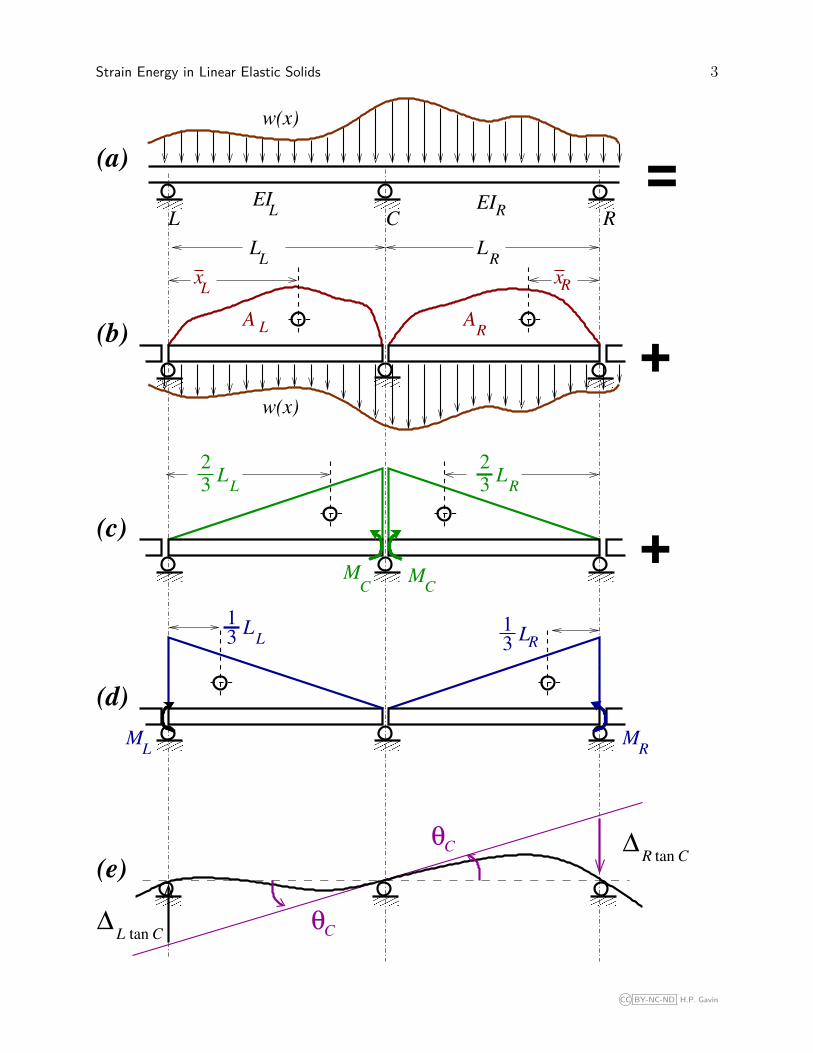
Using the Moment-Area Theorem, we will analyze two adjoining spans of thisbeam to find the relationship between the internal moments at each of thesupports and the loads applied to the beam. We will label the left, center,and right supports of this two-span segment L, C, and R. The left span haslength LL and flexural rigidity EIL; the right span has length LR and flexuralrigidity EIR (see figure (a)).
Applying the principle of superposition to this two-span segment, we canseparate the moments caused by the applied loads from the internal momentsat the supports. The two-span segment can be represented by two simply-supported spans (with zero moment at L, C, and R) carrying the externalloads plus two simply-supported spans carrying the internal moments ML,MC , and MR (figures (b), (c), and (d)). The applied loads are illustratedbelow the beam, so as not to confuse the loads with the moment diagram(shown above the beams). Note that we are being consistent with our signconvention: positive moments create positive curvature in the beam. Theinternal moments ML, MC , and MR are drawn in the positive directions. The
2 CEE 201L. – Uncertainty, Design, and Optimization – Duke University – Spring 2009 – H.P. Gavin
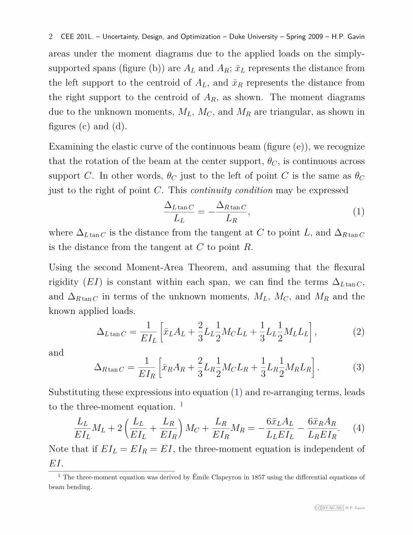
areas under the moment diagrams due to the applied loads on the simply-supported spans (figure (b)) are AL and AR; xL represents the distance fromthe left support to the centroid of AL, and xR represents the distance fromthe right support to the centroid of AR, as shown. The moment diagramsdue to the unknown moments, ML, MC , and MR are triangular, as shown infigures (c) and (d).
Examining the elastic curve of the continuous beam (figure (e)), we recognizethat the rotation of the beam at the center support, θC , is continuous acrosssupport C. In other words, θC just to the left of point C is the same as θC
just to the right of point C. This continuity condition may be expressed∆L tan C
LL= −∆R tan C
LR, (1)
where ∆L tan C is the distance from the tangent at C to point L, and ∆R tan C
is the distance from the tangent at C to point R.
Using the second Moment-Area Theorem, and assuming that the flexuralrigidity (EI) is constant within each span, we can find the terms ∆L tan C ,and ∆R tan C in terms of the unknown moments, ML, MC , and MR and theknown applied loads.
∆L tan C = 1EIL
[xLAL + 2
3LL12MCLL + 1
3LL12MLLL
], (2)
and∆R tan C = 1
EIR
[xRAR + 2
3LR12MCLR + 1
3LR12MRLR
]. (3)
Substituting these expressions into equation (1) and re-arranging terms, leadsto the three-moment equation. 1
LL
EILML + 2
(LL
EIL+ LR
EIR
)MC + LR
EIRMR = −6xLAL
LLEIL− 6xRAR
LREIR. (4)
Note that if EIL = EIR = EI, the three-moment equation is independent ofEI.
1 The three-moment equation was derived by Emile Clapeyron in 1857 using the differential equations ofbeam bending.
CC BY-NC-ND H.P. Gavin
Strain Energy in Linear Elastic Solids 3
���������
���������
���������
���������
���������
���������
������������
���������
���������
���������
���������
������������
������������
���������
���������
���������
���������
���������
���������
������������
��������
������������
��������
∆R tanC
L L
L C REIEI
RL
L
R
C
+
=
+
∆tanCL
3
R
(e)
(c)
(d)
(b)
(a)
w(x)
w(x)
1
3
A L AR
Lx Rx
MC
M
LL
2
3 RL
2
M
RL1
3
ML
LL
θC
θC
CC BY-NC-ND H.P. Gavin
4 CEE 201L. – Uncertainty, Design, and Optimization – Duke University – Spring 2009 – H.P. Gavin
To apply the three-moment equation numerically, the lengths, moments ofinertia, and applied loads must be specified for each span. Two commonlyapplied loads are point loads and uniformly distributed loads. For point loadsPL and PR acting a distance xL and xR from the left and right supports,respectively, the right hand side of the three-moment equation becomes
− 6xLAL
LLEIL− 6xRAR
LREIR= −PL
xL
LLEIL(L2
L − x2L) − PR
xR
LREIR(L2
R − x2R) . (5)
For uniformly distributed loads wL and wR on the left and right spans,
− 6xLAL
LLEIL− 6xRAR
LREIR= −wLL
3L
4EIL− wRL
3R
4EIR. (6)
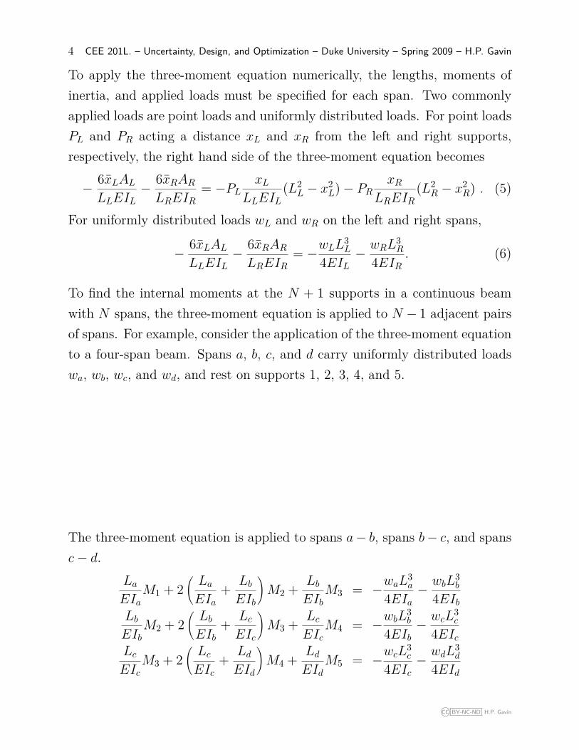
To find the internal moments at the N + 1 supports in a continuous beamwith N spans, the three-moment equation is applied to N − 1 adjacent pairsof spans. For example, consider the application of the three-moment equationto a four-span beam. Spans a, b, c, and d carry uniformly distributed loadswa, wb, wc, and wd, and rest on supports 1, 2, 3, 4, and 5.
The three-moment equation is applied to spans a− b, spans b− c, and spansc− d.
La
EIaM1 + 2
(La
EIa+ Lb
EIb
)M2 + Lb
EIbM3 = −waL
3a
4EIa− wbL
3b
4EIb
Lb
EIbM2 + 2
(Lb
EIb+ Lc
EIc
)M3 + Lc
EIcM4 = −wbL
3b
4EIb− wcL
3c
4EIc
Lc
EIcM3 + 2
(Lc
EIc+ Ld
EId
)M4 + Ld
EIdM5 = −wcL
3c
4EIc− wdL
3d
4EId
CC BY-NC-ND H.P. Gavin

Strain Energy in Linear Elastic Solids 5
We know that M1 = 0 and M5 = 0 because they are at the ends of the span.Applying these end-moment conditions to the three three-moment equationsand casting the equations into matrix form,
1 0 0 0 0
La
EIa2(
La
EIa+ Lb
EIb
)Lb
EIb0 0
0 Lb
EIb2(
Lb
EIb+ Lc
EIc
)Lc
EIc0
0 0 Lc
EIc2(
Lc
EIc+ Ld
EId
)Ld
EId
0 0 0 0 1
M1
M2
M3
M4
M5
=
0
−waL3a
4EIa− wbL3
b
4EIb
−wbL3b
4EIb− wcL3
c
4EIc
−wcL3c
4EIc− wdL3
d
4EId
0
.
(7)The 5 × 5 matrix on the left hand side of equation (7) is called a flexibil-ity matrix and is tri-diagonal and symmetric. This equation can be writtensymbolically as F m = d. By examining the general form of this expression,we can write a matrix representation of the three-moment equation for arbi-trarily many spans. If a numbering convention is adopted in which supportj lies between span j − 1 and span j, the three non-zero elements in row j ofmatrix F are given by
Fj,j−1 = Lj−1
EIj−1, (8)
Fj,j = 2 Lj−1
EIj−1+ Lj
EIj
, (9)
Fj,j+1 = Lj
EIj. (10)
For the case of uniformly distributed loads, row j of vector d is
dj = −wj−1L
3j−1
4EIj−1−wjL
3j
4EIj. (11)
The moments at the supports are computed by solving the system of equa-tions F m = d for the vector m.
CC BY-NC-ND H.P. Gavin
6 CEE 201L. – Uncertainty, Design, and Optimization – Duke University – Spring 2009 – H.P. Gavin
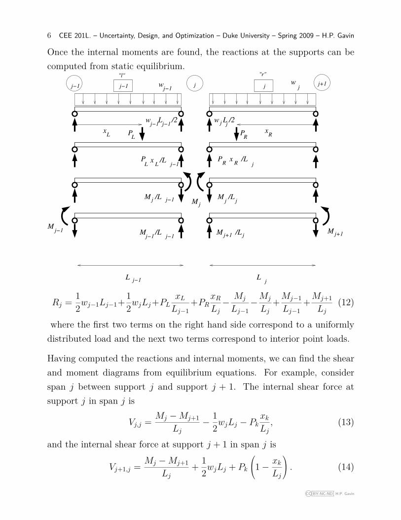
Once the internal moments are found, the reactions at the supports can becomputed from static equilibrium.
j−1 j+1j−1 j
M
M
xxL
PR
PR
xR
/Lj
P /Lj−1L
xL
M/L
j−1/L
j−1M
L j−1 Lj
"l" "r"
P
j−1w
j
w L /2
j
j−1
w
j j
RL
w L /2j−1j−1
jM j−1j
j/L
j
j+1 /L j j+1MM
Rj = 12wj−1Lj−1+ 1
2wjLj +PLxL
Lj−1+PR
xR
Lj− Mj
Lj−1−Mj
Lj+Mj−1
Lj−1+Mj+1
Lj(12)
where the first two terms on the right hand side correspond to a uniformlydistributed load and the next two terms correspond to interior point loads.
Having computed the reactions and internal moments, we can find the shearand moment diagrams from equilibrium equations. For example, considerspan j between support j and support j + 1. The internal shear force atsupport j in span j is
Vj,j = Mj −Mj+1
Lj− 1
2wjLj − Pkxk
Lj, (13)
and the internal shear force at support j + 1 in span j is
Vj+1,j = Mj −Mj+1
Lj+ 1
2wjLj + Pk
1 − xk
Lj
. (14)
CC BY-NC-ND H.P. Gavin
Strain Energy in Linear Elastic Solids 7
The term wjLj/2 in these two equations corresponds to a uniformly dis-tributed load, Pk is a point load within span j, and xk is the distance fromthe right end of span j to the point load Pk.
Beam rotations at the supports may be computed from equations (1), (2),and (3). The slope of the beam at support j is tan θj. From the secondMoment-Area Theorem,
tan θj = − 1EIj
124wjL
3j + 1
6Pkxk
Lj(L2
j − x2k) + 1
3MjLj + 16Mj+1Lj
, (15)
where span j lies between support j and support j + 1. The first term insidethe brackets corresponds to a uniformly distributed load. The second terminside the brackets corresponds to a point load Pk within span j, located adistance xk from the right end of span j, (support j + 1).
CC BY-NC-ND H.P. Gavin
8 CEE 201L. – Uncertainty, Design, and Optimization – Duke University – Spring 2009 – H.P. Gavin
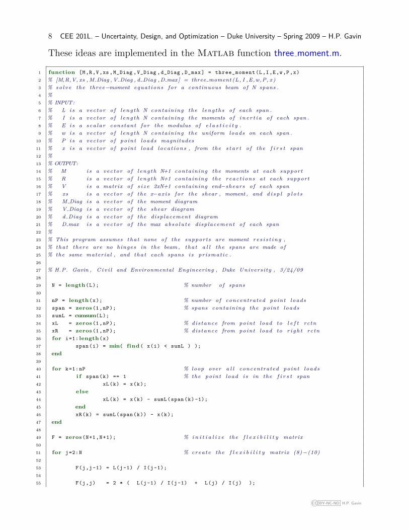
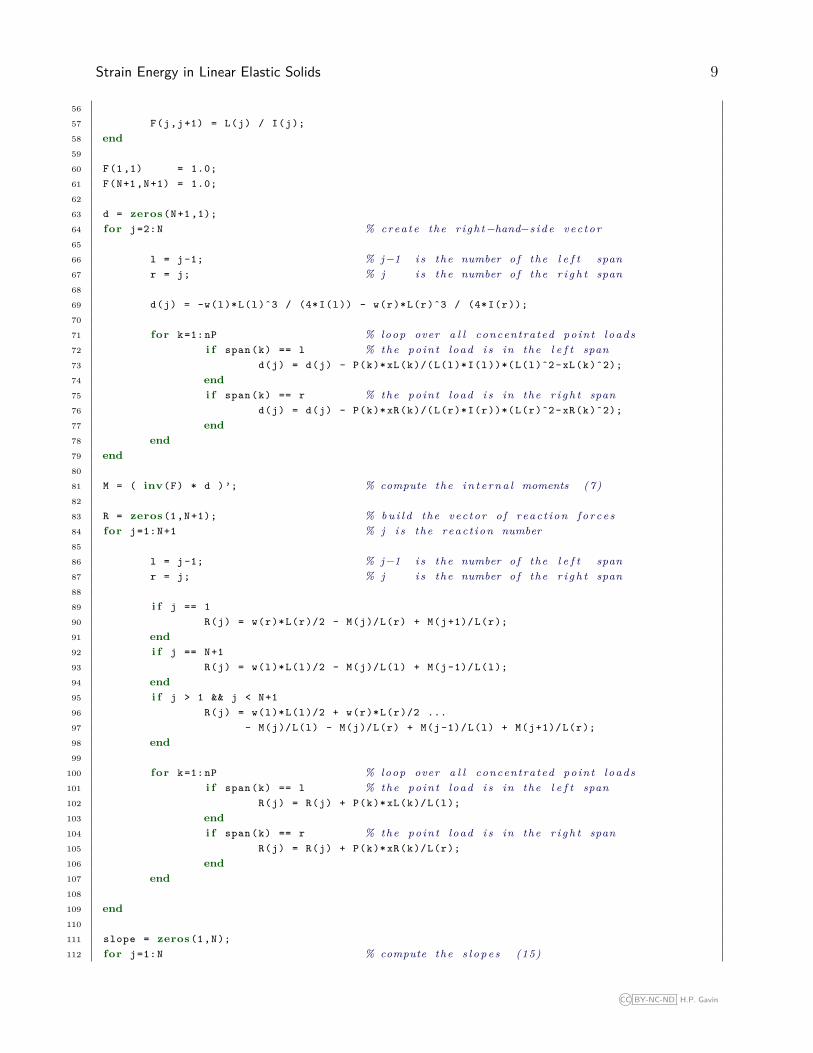
These ideas are implemented in the Matlab function three moment.m.
1 function [M,R,V,xs ,M_Diag ,V_Diag ,d_Diag , D_max ] = three_moment (L,I,E,w,P,x)2 % [M,R,V, xs , M Diag , V Diag , d Diag , D max ] = three moment (L, I ,E,w,P, x )3 % s o l v e the three −moment equat ions f o r a continuous beam of N spans .4 %5 % INPUT:6 % L i s a v e c t o r o f l e n g t h N conta in ing the l e n g t h s o f each span .7 % I i s a v e c t o r o f l e n g t h N conta in ing the moments o f i n e r t i a o f each span .8 % E i s a s c a l a r constant f o r the modulus o f e l a s t i c i t y .9 % w i s a v e c t o r o f l e n g t h N conta in ing the uniform loads on each span .
10 % P i s a ve c t o r o f po in t l oads magnitudes11 % x i s a v e c t o r o f po in t load l o c a t i o n s , from the s t a r t o f the f i r s t span12 %13 % OUTPUT:14 % M i s a v e c t o r o f l e n g t h N+1 conta in ing the moments at each support15 % R i s a v e c t o r o f l e n g t h N+1 conta in ing the r e a c t i o n s at each support16 % V i s a matrix o f s i z e 2xN+1 conta in ing end−shears o f each span17 % xs i s a v e c to r o f the x−a x i s f o r the shear , moment , and d i s p l p l o t s18 % M Diag i s a v ec t o r o f the moment diagram19 % V Diag i s a v e c t o r o f the shear diagram20 % d Diag i s a v e c t o r o f the d isp lacement diagram21 % D max i s a ve c t o r o f the max a b s o l u t e d isp lacement o f each span22 %23 % This program assumes t h a t none o f the suppor t s are moment r e s i s t i n g ,24 % t h a t th ere are no hinges in the beam , t h a t a l l the spans are made o f25 % the same mater ia l , and t h a t each spans i s pr i smat i c .26
27 % H.P. Gavin , C i v i l and Environmental Engineering , Duke Univers i ty , 3/24/0928
29 N = length(L); % number o f spans30
31 nP = length(x); % number o f concentrated po in t l oads32 span = zeros (1,nP ); % spans conta in ing the po in t l oads33 sumL = cumsum(L);34 xL = zeros (1,nP ); % d i s t a n c e from poin t load to l e f t rc tn35 xR = zeros (1,nP ); % d i s t a n c e from poin t load to r i g h t rc tn36 for i=1: length(x)37 span(i) = min( find ( x(i) < sumL ) );38 end39
40 for k=1: nP % loop over a l l concentrated po in t l oads41 i f span(k) == 1 % the po in t load i s in the f i r s t span42 xL(k) = x(k);43 else44 xL(k) = x(k) - sumL(span(k) -1);45 end46 xR(k) = sumL(span(k)) - x(k);47 end48
49 F = zeros(N+1,N+1); % i n i t i a l i z e the f l e x i b i l i t y matrix50
51 for j=2:N % c r e a t e the f l e x i b i l i t y matrix (8) −(10)52
53 F(j,j -1) = L(j -1) / I(j -1);54
55 F(j,j) = 2 * ( L(j -1) / I(j -1) + L(j) / I(j) );
CC BY-NC-ND H.P. Gavin
Strain Energy in Linear Elastic Solids 9
56
57 F(j,j+1) = L(j) / I(j);58 end59
60 F(1 ,1) = 1.0;61 F(N+1,N+1) = 1.0;62
63 d = zeros(N+1 ,1);64 for j=2:N % c r e a t e the r i g h t −hand−s i d e v e c t or65
66 l = j -1; % j −1 i s the number o f the l e f t span67 r = j; % j i s the number o f the r i g h t span68
69 d(j) = -w(l)*L(l)ˆ3 / (4*I(l)) - w(r)*L(r)ˆ3 / (4*I(r));70
71 for k=1: nP % loop over a l l concentrated po in t l oads72 i f span(k) == l % the po in t load i s in the l e f t span73 d(j) = d(j) - P(k)* xL(k)/(L(l)*I(l))*(L(l)ˆ2 - xL(k )ˆ2);74 end75 i f span(k) == r % the po in t load i s in the r i g h t span76 d(j) = d(j) - P(k)* xR(k)/(L(r)*I(r))*(L(r)ˆ2 - xR(k )ˆ2);77 end78 end79 end80
81 M = ( inv(F) * d )’; % compute the i n t e r n a l moments (7)82
83 R = zeros (1,N+1); % b u i l d the v e c t o r o f r e a c t i o n f o r c e s84 for j=1:N+1 % j i s the r e a c t i o n number85
86 l = j -1; % j −1 i s the number o f the l e f t span87 r = j; % j i s the number o f the r i g h t span88
89 i f j == 190 R(j) = w(r)*L(r)/2 - M(j)/L(r) + M(j+1)/L(r);91 end92 i f j == N+193 R(j) = w(l)*L(l)/2 - M(j)/L(l) + M(j -1)/L(l);94 end95 i f j > 1 && j < N+196 R(j) = w(l)*L(l)/2 + w(r)*L(r)/2 ...97 - M(j)/L(l) - M(j)/L(r) + M(j -1)/L(l) + M(j+1)/L(r);98 end99
100 for k=1: nP % loop over a l l concentrated po in t l oads101 i f span(k) == l % the po in t load i s in the l e f t span102 R(j) = R(j) + P(k)* xL(k)/L(l);103 end104 i f span(k) == r % the po in t load i s in the r i g h t span105 R(j) = R(j) + P(k)* xR(k)/L(r);106 end107 end108
109 end110
111 slope = zeros (1,N);112 for j=1:N % compute the s l o p e s (15)
CC BY-NC-ND H.P. Gavin
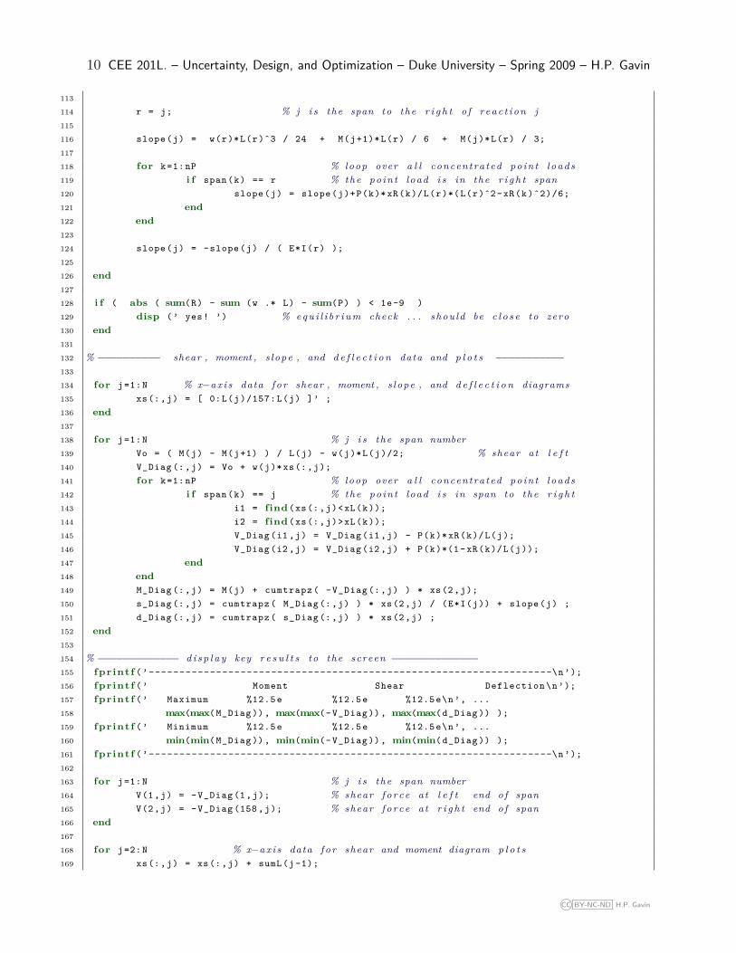
10 CEE 201L. – Uncertainty, Design, and Optimization – Duke University – Spring 2009 – H.P. Gavin
113
114 r = j; % j i s the span to the r i g h t o f r e a c t i o n j115
116 slope (j) = w(r)*L(r)ˆ3 / 24 + M(j+1)*L(r) / 6 + M(j)*L(r) / 3;117
118 for k=1: nP % loop over a l l concentrated po in t l oads119 i f span(k) == r % the po in t load i s in the r i g h t span120 slope (j) = slope (j)+P(k)* xR(k)/L(r)*(L(r)ˆ2 - xR(k )ˆ2)/6;121 end122 end123
124 slope (j) = -slope (j) / ( E*I(r) );125
126 end127
128 i f ( abs ( sum(R) - sum (w .* L) - sum(P) ) < 1e -9 )129 disp (’ yes! ’) % e q u i l i b r i u m check . . . shou ld be c l o s e to zero130 end131
132 % −−−−−−−−−− shear , moment , s lope , and d e f l e c t i o n data and p l o t s −−−−−−−−−−−133
134 for j=1:N % x−a x i s data f o r shear , moment , s lope , and d e f l e c t i o n diagrams135 xs(:,j) = [ 0:L(j )/157: L(j) ]’ ;136 end137
138 for j=1:N % j i s the span number139 Vo = ( M(j) - M(j+1) ) / L(j) - w(j)*L(j)/2; % shear at l e f t140 V_Diag (:,j) = Vo + w(j)* xs(:,j);141 for k=1: nP % loop over a l l concentrated po in t l oads142 i f span(k) == j % the po in t load i s in span to the r i g h t143 i1 = find (xs(:,j)<xL(k));144 i2 = find (xs(:,j)>xL(k));145 V_Diag (i1 ,j) = V_Diag (i1 ,j) - P(k)* xR(k)/L(j);146 V_Diag (i2 ,j) = V_Diag (i2 ,j) + P(k)*(1 - xR(k)/L(j));147 end148 end149 M_Diag (:,j) = M(j) + cumtrapz ( -V_Diag (:,j) ) * xs(2,j);150 s_Diag (:,j) = cumtrapz ( M_Diag (:,j) ) * xs(2,j) / (E*I(j)) + slope (j) ;151 d_Diag (:,j) = cumtrapz ( s_Diag (:,j) ) * xs(2,j) ;152 end153
154 % −−−−−−−−−−−−− d i s p l a y key r e s u l t s to the screen −−−−−−−−−−−−−−155 fpr intf (’ ------------------------------------------------------------------\n’);156 fpr intf (’ Moment Shear Deflection \n’);157 fpr intf (’ Maximum %12.5 e %12.5 e %12.5 e\n’, ...158 max(max( M_Diag )), max(max(- V_Diag )), max(max( d_Diag )) );159 fpr intf (’ Minimum %12.5 e %12.5 e %12.5 e\n’, ...160 min(min( M_Diag )), min(min(- V_Diag )), min(min( d_Diag )) );161 fpr intf (’ ------------------------------------------------------------------\n’);162
163 for j=1:N % j i s the span number164 V(1,j) = -V_Diag (1,j); % shear f o r c e at l e f t end o f span165 V(2,j) = -V_Diag (158 ,j); % shear f o r c e at r i g h t end o f span166 end167
168 for j=2:N % x−a x i s data f o r shear and moment diagram p l o t s169 xs(:,j) = xs(:,j) + sumL(j -1);
CC BY-NC-ND H.P. Gavin
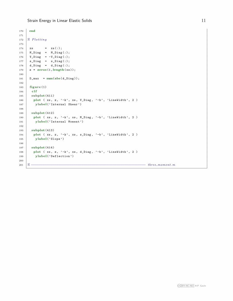
Strain Energy in Linear Elastic Solids 11
170 end171
172 % P l o t t i n g173
174 xs = xs (:);175 M_Diag = M_Diag (:);176 V_Diag = -V_Diag (:);177 s_Diag = s_Diag (:);178 d_Diag = d_Diag (:);179 z = zeros (1, length(xs ));180
181 D_max = max(abs( d_Diag ));182
183 figure (1)184 c l f185 subplot (411)186 plot ( xs , z, ’-k’, xs , V_Diag , ’-b’, ’LineWidth ’, 2 )187 ylabel (’Internal Shear ’)188
189 subplot (412)190 plot ( xs , z, ’-k’, xs , M_Diag , ’-b’, ’LineWidth ’, 2 )191 ylabel (’Internal Moment ’)192
193 subplot (413)194 plot ( xs , z, ’-k’, xs , s_Diag , ’-b’, ’LineWidth ’, 2 )195 ylabel (’Slope ’)196
197 subplot (414)198 plot ( xs , z, ’-k’, xs , d_Diag , ’-b’, ’LineWidth ’, 2 )199 ylabel (’Deflection ’)200
201 % −−−−−−−−−−−−−−−−−−−−−−−−−−−−−−−−−−−−−−−−−−−−−−−−−−−−−−−−−−− three moment .m
CC BY-NC-ND H.P. Gavin
12 CEE 201L. – Uncertainty, Design, and Optimization – Duke University – Spring 2009 – H.P. Gavin
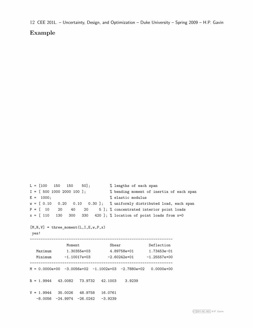
Example
L = [100 150 150 50]; % lengths of each spanI = [ 500 1000 2000 100 ]; % bending moment of inertia of each spanE = 1000; % elastic modulusw = [ 0.10 0.20 0.10 0.30 ]; % uniformly distributed load, each spanP = [ 10 20 40 20 5 ]; % concentrated interior point loadsx = [ 110 130 300 330 420 ]; % location of point loads from x=0
[M,R,V] = three_moment(L,I,E,w,P,x)yes!
------------------------------------------------------------------Moment Shear Deflection
Maximum 1.30355e+03 4.89758e+01 1.73453e-01Minimum -1.10017e+03 -2.60242e+01 -1.25557e+00
------------------------------------------------------------------M = 0.0000e+00 -3.0056e+02 -1.1002e+03 -2.7880e+02 0.0000e+00
R = 1.9944 43.0082 73.9732 42.1003 3.9239
V = 1.9944 35.0026 48.9758 16.0761-8.0056 -24.9974 -26.0242 -3.9239
CC BY-NC-ND H.P. Gavin
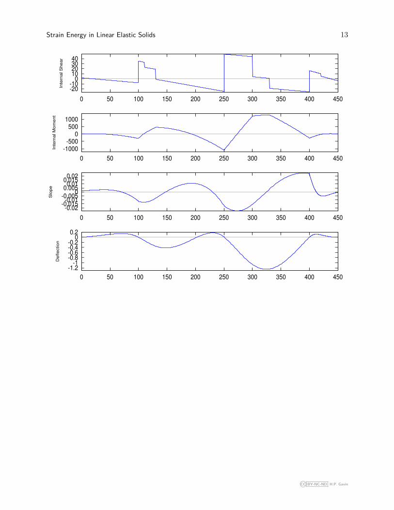
Strain Energy in Linear Elastic Solids 13
-20-10
010203040
0 50 100 150 200 250 300 350 400 450
Inte
rna
l S
he
ar
-1000-500
0500
1000
0 50 100 150 200 250 300 350 400 450
Inte
rna
l M
om
en
t
-0.02-0.015-0.01
-0.0050
0.0050.01
0.0150.02
0 50 100 150 200 250 300 350 400 450
Slo
pe
-1.2-1
-0.8-0.6-0.4-0.2
00.2
0 50 100 150 200 250 300 350 400 450
De
fle
ctio
n
CC BY-NC-ND H.P. Gavin
Related Documents