HAL Id: hal-02969300 https://hal.archives-ouvertes.fr/hal-02969300 Submitted on 16 Oct 2020 HAL is a multi-disciplinary open access archive for the deposit and dissemination of sci- entific research documents, whether they are pub- lished or not. The documents may come from teaching and research institutions in France or abroad, or from public or private research centers. L’archive ouverte pluridisciplinaire HAL, est destinée au dépôt et à la diffusion de documents scientifiques de niveau recherche, publiés ou non, émanant des établissements d’enseignement et de recherche français ou étrangers, des laboratoires publics ou privés. The third realization of the International Celestial Reference Frame by very long baseline interferometry P. Charlot, C. S Jacobs, D. Gordon, Sébastien Lambert, A. de Witt, J. Böhm, A. L Fey, R. Heinkelmann, E. Skurikhina, O. Titov, et al. To cite this version: P. Charlot, C. S Jacobs, D. Gordon, Sébastien Lambert, A. de Witt, et al.. The third realization of the International Celestial Reference Frame by very long baseline interferometry. Astronomy and As- trophysics - A&A, EDP Sciences, 2020, 644, pp.A159. 10.1051/0004-6361/202038368. hal-02969300

Welcome message from author
This document is posted to help you gain knowledge. Please leave a comment to let me know what you think about it! Share it to your friends and learn new things together.
Transcript
HAL Id: hal-02969300https://hal.archives-ouvertes.fr/hal-02969300
Submitted on 16 Oct 2020
HAL is a multi-disciplinary open accessarchive for the deposit and dissemination of sci-entific research documents, whether they are pub-lished or not. The documents may come fromteaching and research institutions in France orabroad, or from public or private research centers.
L’archive ouverte pluridisciplinaire HAL, estdestinée au dépôt et à la diffusion de documentsscientifiques de niveau recherche, publiés ou non,émanant des établissements d’enseignement et derecherche français ou étrangers, des laboratoirespublics ou privés.
The third realization of the International CelestialReference Frame by very long baseline interferometry
P. Charlot, C. S Jacobs, D. Gordon, Sébastien Lambert, A. de Witt, J. Böhm,A. L Fey, R. Heinkelmann, E. Skurikhina, O. Titov, et al.
To cite this version:P. Charlot, C. S Jacobs, D. Gordon, Sébastien Lambert, A. de Witt, et al.. The third realization ofthe International Celestial Reference Frame by very long baseline interferometry. Astronomy and As-trophysics - A&A, EDP Sciences, 2020, 644, pp.A159. �10.1051/0004-6361/202038368�. �hal-02969300�
Astronomy & Astrophysics manuscript no. icrf3 c©ESO 2020September 10, 2020
The third realization of the International Celestial Reference Frameby very long baseline interferometry
P. Charlot1, C. S. Jacobs2, D. Gordon3, S. Lambert4, A. de Witt5, J. Böhm6, A. L. Fey7, R. Heinkelmann8,E. Skurikhina9, O. Titov10, E. F. Arias4, S. Bolotin3, G. Bourda1, C. Ma11?, Z. Malkin12, 13, A. Nothnagel14??,
D. Mayer6???, D. S. MacMillan3, T. Nilsson8????, and R. Gaume15
1 Laboratoire d’astrophysique de Bordeaux, Univ. Bordeaux, CNRS, B18N, Allée Geoffroy Saint-Hilaire, 33615 Pessac, Francee-mail: [email protected]
2 Jet Propulsion Laboratory, California Institute of Technology, 4800 Oak Grove Drive, Pasadena, CA 91109-8099, USA3 NVI Inc. at NASA Goddard Space Flight Center, Code 61A.1, Greenbelt, MD 20771, USA4 SYRTE, Observatoire de Paris, Université PSL, CNRS, Sorbonne Université, LNE, 61 Av. de l’Observatoire, 75014 Paris, France5 Hartebeesthoek Radio Astronomy Observatory, PO Box 443, Krugersdorp 1740, South Africa6 Department of Geodesy and Geoinformation, Technische Universität Wien, Wiedner Hauptstraße 8-10, 1040 Vienna, Austria7 U.S. Naval Observatory, 3450 Massachusetts Avenue NW, Washington, DC 20392-5420, USA8 Helmholtz Centre Potsdam, German Research Centre for Geosciences, Telegrafenberg, A17, D-14473 Potsdam, Germany9 Institute of Applied Astronomy, Russian Academy of Sciences, Nab. Kutuzova 10, St. Petersburg 191187, Russia
10 Geoscience Australia, P.O. Box 378, Canberra, ACT 2601, Australia11 NASA Goddard Space Flight Center, Code 61A.1, Greenbelt, MD 20771, USA12 Pulkovo Observatory, St. Petersburg 196140, Russia13 Kazan Federal University, Kazan 420000, Russia14 Institut für Geodäsie und Geoinformation, Universät Bonn, Nußallee 17, D-53115 Bonn, Germany15 National Science Foundation, 2415 Eisenhower Avenue, Alexandria, Virginia 22314, USA
Received 7 May 2020 / Accepted 31 July 2020
ABSTRACT
A new realization of the International Celestial Reference Frame (ICRF) is presented based on the work achieved by a working groupof the International Astronomical Union (IAU) mandated for this purpose. This new realization follows the initial realization of theICRF completed in 1997 and its successor, ICRF2, adopted as a replacement in 2009. The new frame, referred to as ICRF3, is basedon nearly 40 years of data acquired by very long baseline interferometry at the standard geodetic and astrometric radio frequencies(8.4 and 2.3 GHz), supplemented with data collected at higher radio frequencies (24 GHz and dual-frequency 32 and 8.4 GHz) over thepast 15 years. State-of-the-art astronomical and geophysical modeling has been used to analyze these data and derive source positions.The modeling integrates, for the first time, the effect of the galactocentric acceleration of the solar system (directly estimated from thedata) which, if not considered, induces significant deformation of the frame due to the data span. The new frame includes positions at8.4 GHz for 4536 extragalactic sources. Of these, 303 sources, uniformly distributed on the sky, are identified as “defining sources”and as such serve to define the axes of the frame. Positions at 8.4 GHz are supplemented with positions at 24 GHz for 824 sources andat 32 GHz for 678 sources. In all, ICRF3 comprises 4588 sources, with three-frequency positions available for 600 of these. Sourcepositions have been determined independently at each of the frequencies in order to preserve the underlying astrophysical contentbehind such positions. They are reported for epoch 2015.0 and must be propagated for observations at other epochs for the mostaccurate needs, accounting for the acceleration toward the Galactic center, which results in a dipolar proper motion field of amplitude0.0058 milliarcsecond/yr (mas/yr). The frame is aligned onto the International Celestial Reference System to within the accuracy ofICRF2 and shows a median positional uncertainty of about 0.1 mas in right ascension and 0.2 mas in declination, with a noise floorof 0.03 mas in the individual source coordinates. A subset of 500 sources is found to have extremely accurate positions, in the rangeof 0.03 to 0.06 mas, at the traditional 8.4 GHz frequency. Comparing ICRF3 with the recently released Gaia Celestial ReferenceFrame 2 in the optical domain, there is no evidence for deformations larger than 0.03 mas between the two frames, in agreement withthe ICRF3 noise level. Significant positional offsets between the three ICRF3 frequencies are detected for about 5% of the sources.Moreover, a notable fraction (22%) of the sources shows optical and radio positions that are significantly offset. There are indicationsthat these positional offsets may be the manifestation of extended source structures. This third realization of the ICRF was adopted bythe IAU at its 30th General Assembly in August 2018 and replaced the previous realization, ICRF2, on January 1, 2019.
Key words. Reference systems – Astrometry – Techniques: interferometric – Galaxies: quasars: general – Galaxies: nuclei – Radiocontinuum: general
? Retired?? Now at Technische Universität Wien, Vienna, Austria
??? Now at Federal Office of Metrology and Surveying, Vienna, Austria???? Now at Lantmäteriet – The Swedish mapping, cadastral and land
registration authority, Geodetic Infrastructure, Gävle, Sweden
1. Introduction
The International Celestial Reference Frame (ICRF) and its suc-cessor, ICRF2, have been the basis for high-accuracy astrome-try for more than two decades. Both frames have drawn on si-
Article number, page 1 of 28
A&A proofs: manuscript no. icrf3
multaneous 8.4 GHz and 2.3 GHz observations of compact ex-tragalactic radio sources acquired by very long baseline inter-ferometry (VLBI), starting from the end of the 1970s. The pri-mary frequency in this observing scheme is 8.4 GHz (X band),while 2.3 GHz (S band) is only used for ionosphere calibration.Hereafter, such dual-frequency VLBI observations are referredto as S/X band, following the standard designation.
The ICRF (Ma et al. 1998) was the first all-sky realization ofan extragalactic frame with milliarcsecond (mas) position accu-racy and the first realization of the International Celestial Refer-ence System (ICRS) (Arias et al. 1995). It was adopted by theInternational Astronomical Union (IAU) at its 23rd General As-sembly in 1997, replacing the Fifth Fundamental Catalog of stars(FK5) (Fricke et al. 1988) as the fundamental celestial referenceframe as of January 1, 1998. Unlike previously (e.g., for the FK5or other stellar frames), the definition of the frame axes was nolonger related to the equinox and equator but relied on coordi-nates of so-called defining sources. The ICRF included 212 suchdefining sources out of a total of 608 objects for which positionswere reported. The orientation of the ICRF axes was deemedto be accurate to 20 microarcseconds (µas) while source coordi-nates had a noise floor of 250 µas. As a consequence of the ICRSdefinition, all source positions in the ICRF were independent ofepoch. The release of ICRF was a major step forward and as suchit became the required passage to link other celestial referenceframes to the ICRS, among which were the dynamical frame(Standish 1998) and the Hipparcos stellar frame (Kovalevskyet al. 1997). The ICRF has also allowed for many advances inother fields, such as geodesy and Earth orientation studies, orrelated to practical applications like deep space navigation.
As time passed, VLBI observing networks and technologyimproved and further sources were observed. On the geodesyside, observations became organized in a formal way under theumbrella of the International VLBI Service for Geodesy and As-trometry (IVS), established in 1999 (Schlüter & Behrend 2007),permitting more resources to be pooled together. Two ICRF ex-tensions, ICRF-Ext.1 and ICRF-Ext.2, were constructed in 2000and 2002, adding another 109 sources to the frame (Fey et al.2004). At the same time, systematic surveys of the VLBI skywere initiated using the Very Long Baseline Array (VLBA)1, en-larging the pool of VLBI sources with milliarcsecond-accuratepositions to more than a thousand (Beasley et al. 2002). By themid 2000s, it was realized that the amount of data, their accu-racy, and the denser sky coverage, along with modeling improve-ments since ICRF was delivered, would justify the building of anew reference frame to get the full potential of the available datasets. This prompted the construction of the second realizationof the ICRF, named ICRF2, which was completed in 2009 andadopted by the IAU at its 27th General Assembly in the sameyear (Fey et al. 2015). As a result, ICRF2 replaced ICRF on Jan-uary 1, 2010. The new realization comprises 3414 sources, ofwhich 295 are defining sources. The orientation of its axes isknown to 10 µas, while source coordinates have a noise floor of40 µas. The large increase in the number of sources from ICRF toICRF2 (a factor of six) was largely due to the inclusion of obser-vations from a series of VLBA Calibrator Survey (VCS) astro-metric campaigns carried out between 1994 and 2007 (Beasleyet al. 2002; Fomalont et al. 2003; Petrov et al. 2005, 2006; Ko-valev et al. 2007; Petrov et al. 2008). The goal of these was toexpand the pool of calibrators available for VLBI observations inphase-referencing mode (Beasley & Conway 1995). Such cam-
1 The VLBA is a facility of the National Science Foundation operatedunder cooperative agreement by Associated Universities, Inc.
paigns added nearly 2200 sources exclusively observed by theVLBA to the catalog of sources derived from IVS sessions. TheVCS sources, still, had position uncertainties typically five timeslarger than the other sources due to being observed in surveymode and generally only in a single session. For this reason, theywere categorized separately from the IVS sources in ICRF2.
Since the release of ICRF2, the VLBI database has contin-ued to expand thanks to ongoing observing programs run by theIVS but also through specific projects carried out independently,notably by using the VLBA. The latter includes a complete re-observation of all VCS sources in 2014–2015, which has broughtan overall factor of five improvement in coordinate uncertainties,hence bringing position uncertainties for the VCS sources closerto those for the rest of the ICRF2 sources (Gordon et al. 2016).A specific effort has also been made to strengthen observationsof optically bright ICRF2 sources within IVS programs to facil-itate the alignment of the optical reference frame which is beingbuilt by the Gaia space mission (Le Bail et al. 2016). At thesame time, VLBI observations at higher radio frequencies beganto develop, namely at 24 GHz (K band) and 32 GHz (Ka band),the latter with simultaneous X band observations for ionospherecalibration (hence the usual X/Ka band designation for this dual-frequency observing scheme). An initial catalog of 268 sources,together with VLBI images of the sources, was produced usingthe VLBA at K band (Lanyi et al. 2010; Charlot et al. 2010),while positions for 482 sources were reported at X/Ka band fromobservations with the Deep Space Network (DSN) (Jacobs et al.2012). Despite the limited data sets, both catalogs showed anoverall agreement with ICRF2 at the 300 µas level when compar-ing individual source coordinates, hence revealing the value ofsuch high-frequency observations. By 2012, the wealth of the ad-ditional VLBI data already acquired, or foreseen, together withthe need to have a state-of-the-art VLBI frame to align as wellas possible the future Gaia optical frame onto the ICRS, createdthe necessary motivation for generating a new realization of theICRF. Shortly after the 28th General Assembly of the IAU inBeijing, a working group under IAU Division A was assembledto this end. The mandate of the working group was to generatethe third realization of the ICRF by 2018, for adoption at the30th IAU General Assembly to take place that year.
The work accomplished toward the generation of the thirdrealization of the ICRF, hereafter referred to as ICRF3, was or-ganized along several lines. One such line was aimed at acquir-ing new appropriate data to correct deficiencies of ICRF2. Inthis respect, the focus was placed not so much on trying to in-crease the number of sources but rather on improving uniformityand internal consistency. The campaign to re-observe all VCSsources (Gordon et al. 2016) falls into this line. As noted above,this campaign vastly improved coordinate uncertainties for therelevant 2200 such sources, resulting in an overall distributionof source position uncertainties that is now much more uniform.Specific efforts were also targeted to strengthen observations inthe far south (i.e., for declinations below −45◦). However, thelimited number of VLBI telescopes in the Southern Hemisphereremains as a major bottleneck to reach the same quality in thatarea of the sky (in terms of source density and position accuracy)as that available further north. The full data set used to generateICRF3 is described in Sect. 2. Compared to ICRF and ICRF2, anew feature is the inclusion of data at K band and X/Ka band inaddition to those at the standard S/X band geodetic frequencies.The resulting three-frequency positions (at X, K, and Ka band)are herewith reported as part of ICRF3 without being combinedin order to preserve the underlying astrophysical information.
Article number, page 2 of 28
P. Charlot et al.: The third realization of the International Celestial Reference Frame
Another major activity of the working group consisted ingenerating ICRF3 prototype realizations at several stages of thework. These allowed the group to study the impact of data sets,astronomical and geophysical modeling, analysis configuration,software packages, and individuals that analyze the data on theresulting frame. In practice, such prototype realizations wereproduced at eight different institutions2 in Australia, Austria,France, Germany, Russia, and USA using five different softwarepackages. Of interest is that one such ICRF3 prototype realiza-tion was delivered to the Gaia science team in July 2017 and usedin the process to generate the catalog for the Gaia Data Release 2(Gaia DR2) in order to align the Gaia frame with the ICRS (Lin-degren et al. 2018). The final solution for ICRF3 incorporatesdata up to spring 2018 and was produced in July 2018. Section 3below reviews the adopted modeling and analysis configuration,while Sect. 4 describes the alternate analyses that have been con-ducted to assess errors in ICRF3. A newly added feature in themodeling is the galactocentric acceleration of the solar system,long sought and first detected by Titov et al. (2011). With a mag-nitude of about 5 µas/yr, this effect produces detectable apparentdrifts in the source positions, especially over the almost 40-yearspan now reached by the S/X band data. Unlike previously (i.e.,for ICRF and ICRF2), the source coordinates in ICRF3 are re-ferred to a specific epoch and hence should be properly propa-gated for epochs away from that reference epoch, accounting forGalactic acceleration, for the most demanding needs.
Details of ICRF3 are given in Sect. 5, including source cate-gorization and tables of positions reported separately at X band,K band, and Ka band. The frame has a new set of definingsources selected in a way to be uniformly distributed on the sky.Recommendations to future users on how to use the catalogedICRF3 positions, depending on their needs, are also provided.Section 6 makes an assessment of the alignment of ICRF3 ontoICRS, emphasizes the improvement and benefits of the new re-alization over ICRF2, and compares ICRF3 with the Gaia DR2celestial reference frame (Gaia-CRF2), which is the first extra-galactic frame ever built in the optical domain (Gaia Collabora-tion et al. 2018). Consistency between multi-frequency radio po-sitions and between radio and optical positions is also addressedas part of that section. The final sections outline the adoptionprocess by the IAU and the future evolution of the ICRF.
2. Observations
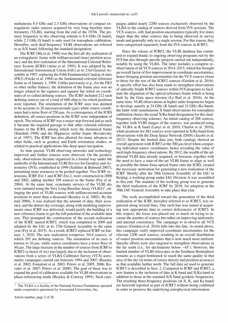
The VLBI data used to build ICRF3 were acquired by arraysof 2 to 20 radiotelescopes organized in their vast majority un-der the umbrella of the IVS, the VLBA, and the DSN. Overthe years, a total of 167 telescopes, located on 126 differentsites, participated in such VLBI sessions (Fig. 1). Observationswere carried out using the so-called bandwidth synthesis mode,which permits the determination of precise group delay quan-tities by observing multiple channels spread out across a band-width of several hundred MHz, as originally devised by Rogers(1970). Following acquisition, the data were processed at oneof the IVS correlators (in Bonn, Haystack, Kashima, Shang-hai, Vienna, or Washington), the VLBA correlator in Soccoro,the Australia Telescope National Facility correlator in Perth, orthe DSN processor in Pasadena. Post-processing was accom-plished by calibrating the raw phases to make them consistent2 Geoscience Australia (Australia), Technische Universität Wien (Aus-tria), Observatoire de Paris (France), Helmholtz Centre Potsdam (Ger-many), Institute of Applied Astronomy St. Petersburg (Russia), NASAGoddard Space Flight Center (USA), Jet Propulsion Laboratory (USA),U.S. Naval Observatory (USA).
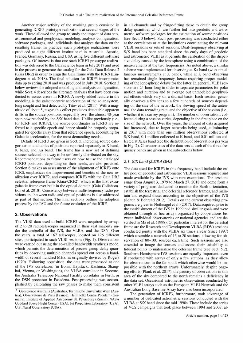
in all channels and by fringe-fitting these to obtain the groupdelay quantities which are further fed into geodetic and astro-metric software packages for the estimation of source positions(see Sect. 3 below). Such post-processing was conducted eitherat the correlators or at the institutions coordinating the relevantVLBI sessions or sets of sessions. Dual-frequency observing atS/X band has been standard since the early days of geodeticand astrometric VLBI as it permits the calibration of the disper-sive delay caused by the ionosphere using a combination of themeasurements at the two frequencies. As noted above, a similarscheme was implemented for observing at Ka band (with simul-taneous measurements at X band), while at K band observinghas remained single-frequency, hence requiring proper model-ing of the ionospheric delays for the latter. In general, VLBI ses-sions are 24-hour long in order to separate parameters for polarmotion and nutation and to average out unmodeled geophysi-cal effects which vary on a diurnal basis. Each session gener-ally observes a few tens to a few hundreds of sources depend-ing on the size of the network, the slewing speed of the anten-nas, the data recording rate, and the objective of the session (i.e.,whether it is a survey program). The number of observations col-lected during a session varies, depending in the first place on thesize of the network. Over the years, the amount of data acquiredhas increased, due to larger networks being used, culminatingin 2017 with more than one million observations collected atS/X band, 0.1 million collected at K band, and 0.01 million col-lected at X/Ka band (see the distribution of observations per yearin Fig. 2). Characteristics of the data sets at each of the three fre-quency bands are given in the subsections below.
2.1. S/X band (2.3/8.4 GHz)
The data used for ICRF3 in this frequency band include the en-tire pool of geodetic and astrometric VLBI sessions acquired andmade available by the IVS with rare exceptions. The sessionsrange from August 3, 1979 to March 27, 2018 and come from avariety of programs dedicated to monitor the Earth orientation,establish the terrestrial and celestial reference frames, and main-tain and expand these, according to the objectives of the IVS(Schuh & Behrend 2012). Details on the current observing pro-grams are given in Nothnagel et al. (2017). Data acquired prior tothe establishment of the IVS in 1999 had similar goals and wereobtained through ad hoc arrays organized by cooperations be-tween individual observatories or national agencies and are de-scribed in Ma et al. (1998). Of particular interest for the celestialframe are the Research and Development VLBA (RDV) sessionsconducted jointly with the VLBA six times a year (since 1997)which assemble a network of 15 to 20 stations, allowing for ob-servation of 80–100 sources each time. Such sessions are alsoessential to image the sources and assess their suitability asfiducial points to materialize the celestial frame (see Sect. 5.2).Southern-Hemisphere IVS sessions are equally important, evenif conducted with arrays of only a few stations, as they allowfor observations in the far south which otherwise would be im-possible with the northern arrays. Unfortunately, despite ongo-ing efforts (Plank et al. 2017), the paucity of observations in thisarea of the sky compared to the north remains a deficiency inthe data set. Occasional astrometric observations conducted byother VLBI arrays such as the European VLBI Network and theAustralian Long Baseline Array have also been incorporated.
The generation of ICRF3, furthermore, took advantage ofa number of dedicated astrometric sessions conducted with theVLBA at S/X band since the mid 1990s. These include the seriesof VCS campaigns that took place between 1994 and 2007, al-
Article number, page 3 of 28
A&A proofs: manuscript no. icrf3
-60°
-30°
0°
+30°
+60°
-120° -60° 0° +60° +120°
Ch
Cn
Ys/Yj/Yb
65/6a/Ro/61/54/55
Bs
Hf
Az
Ft
Oh
Sc
Be
Mg
St
Se
Wf/Hs/Ss
Hn
Tc
Sb
Gg/GfMd
Ap
G3/Gn/Gb/G1
Ri/Mi
Cg
BoNl
Le
AuMt
Hr/H7 Fd
Pl
Ms
La
Ve
Yk/Ye
El
Pe
BrS1Vi
Wt
Ya
SoGc
Ko
Hk
Mk
Kk/Ku
Sn
Nm
Ww
Kw
Mr
45/Ti/34/35/36
Pa
Ho/Hb
Cc
S3/Si
Ke
Kv
VsSh
T6
Yg
Km
Bd
UrZc
Sy
Sm
Sv
Hh/Ht
Mh/Mv
Tn
Ma
Nt
KiKr
Wz/Wn/Tg
Tl
On
Ny
Mc
Hp
Hg
Gr
EbTo
+30°
+35°
+40°
-120° -110°
Mt
Hr/H7 Fd
Pl
La
Pt
Ve
Kp
Fl
Yu
El
Bb
Oc
Dm
MePn
Mo/Mq13/Gv
15/1425/26
PbJ1
Ml
Oo/OrOv
PvSp
Vb
Qu
Hc
Fs/Fo
PfPr
+35°
+40°
+130° +140°
S3/Si
MzVm/Mn
Ka/Kb/K1Is
Ts/Tk
KzTa/MuKg/K3
N6Ud
My
Uc
Ai
Fig. 1. World map showing the geographical location of the 167 antennas (situated on 126 different sites) that participated in the observations usedfor ICRF3. The red dots show the antennas from the IVS network (and pre-existing adhoc VLBI arrays that observed at S/X band), the blue onesthose from the VLBA, and the yellow ones those from the DSN and ESA. The two-character codes printed near each dot correspond to the shortnames of the antennas, as defined in the IVS nomenclature. The two insets show enlargements of western US and Japan where a large number ofantennas (including mobile VLBI stations) have been used to collect geodetic VLBI data over the years due to the seismic nature of these regions.
Fig. 2. Distribution of the observations used for ICRF3. The three his-tograms show the number of VLBI delays per year at S/X band (upperpanel), K band (middle panel), and X/Ka band (lower panel). For ease ofreading, the number of observations is plotted with a logarithmic scale.
ready incorporated in ICRF2 (see Fey et al. 2015), along with thecampaign that re-observed all VCS sources in 2014–2015, whichwas initiated specifically for the purpose of ICRF3, as reportedin Gordon et al. (2016). More recently, another 24 such VLBAsessions have been run under the US Naval Observatory share ofthe VLBA observing time. Those sessions targeted all sourcesin the VLBI pool meeting one of the following criteria: (i) hadnot been observed since 2009 (i.e., when ICRF2 was delivered),(ii) had less than 50 observations, (iii) were observed in threeor fewer sessions, or (iv) were among the weakest known opti-
cally bright sources listed in Le Bail et al. (2016). The goal herewas to further enhance uniformity of the data sets for ICRF3.In all, the VLBA sessions constitute only a small portion of theentire set of S/X band sessions (200 sessions out of a total of6206 sessions) but account for 26% of the data, while more thantwo-thirds (68%) of the sources have observations coming ex-clusively from the VLBA. See Gordon (2017) for further detailson the impact of the VLBA observing on the celestial frame.
2.2. K band (24 GHz)
The data sets in this band are made of 40 VLBA sessions thatobserved the northern sky (down to mid-southern declinations),supplemented with 16 single-baseline sessions between tele-scopes in Hartebeesthoek (South Africa) and Hobart (Australia)that observed sources below −15◦ declination (down to the farsouth). The first VLBA session was conducted on May 15, 2002and was part of a set of ten such sessions that ultimately led tothe first realization of a celestial frame in this frequency band,although not covering the entire sky (Lanyi et al. 2010). Apartfrom two similar follow-up sessions in 2008, VLBA observingwas then interrupted until 2015, after which it was started again(see Fig. 2). Since then, another 25 VLBA sessions have beencarried out, the bulk of which were run in 2017–2018 underthe US Naval Observatory share of the VLBA observing time.The latest session incorporated in this work was conducted onMay 5, 2018. Additionally, three archived VLBA sessions ded-icated to observing sources in the Galactic plane (Petrov et al.2011) were also included. Observations between Hartebeesthoekand Hobart were initiated at about the same time as the VLBAsessions restarted (first session run on May 4, 2014) to completethe sky coverage in the far south. One southern session also in-cluded the Tianma 65 m telescope near Shanghai (China) while
Article number, page 4 of 28
P. Charlot et al.: The third realization of the International Celestial Reference Frame
another one included the Tidbinbilla 70 m telescope near Can-berra (Australia). In all, the VLBA sessions account for 99% ofthe data while the Southern-Hemisphere sessions account for 1%of it, which leads to a majority of sources (66%) having onlyVLBA observations, a similar division as that at S/X band.
2.3. X/Ka band (8.4/32 GHz)
Observations at X/Ka band were initiated in 2005 with the pri-mary goal of building a reference frame for spacecraft naviga-tion, now conducted on the DSN using the Ka frequency band.The data set includes a total of 168 single-baseline sessions thatinvolved seven telescopes at the three DSN sites in Goldstone(California), Robledo (Spain), and Tidbinbilla (Australia). Thefirst of these sessions took place on July 9, 2005 while the mostrecent one incorporated was run on January 28, 2018. Occasion-ally (in about 10% of the sessions), the European Space Agency(ESA) telescope in Malargüe (Argentina) joined the observa-tions, which was essential to improve the north-south geometryof the network and reduce systematics in the reference frame.
3. Analysis
The principle behind VLBI data analysis is to compare measuredquantities with a priori theoretical modeling of the same quan-tities and to refine underlying models by estimating model pa-rameter corrections that best fit the data. Depending on the ob-jective pursued, such parameters may pertain to the entire dataset (e.g., station positions and velocities, source positions,...) oronly to individual sessions (e.g., the Earth orientation param-eters,...) or even to a small portion of a session (e.g., clock andtroposphere parameters which vary on the order of hours). Least-squares methods are generally employed for this estimation. TheVLBI modeling, analysis configuration, and software packagesused to produce ICRF3 are outlined in the following sections.
3.1. Astronomical, geophysical, and instrumental modeling
The measured VLBI quantities (group delay and delay rate) usedfor ICRF3 were analyzed employing state-of-the-art astronomi-cal and geophysical modeling, generally following the prescrip-tions of the International Earth Rotation and Reference SystemsService (IERS) (Petit & Luzum 2010). An extensive review of allthe effects to be incorporated in the VLBI model in order to reachthe highest accuracy is given in Sovers et al. (1998). Apart fromthe effect induced by the galactocentric acceleration of the solarsystem, only brief information, primarily to identify the modelsselected, is thus provided here. The interested reader is referredto the Sovers et al. (1998) review for details on the underlyingphysics. Galactocentric acceleration is addressed specifically inSect. 3.2 as it is the first time this effect is introduced in the mod-eling used to generate a VLBI celestial reference frame.
The geometric portion of the VLBI delay, including relativis-tic effects, was derived consistently with the so-called consensusmodel (Eubanks 1991) which provides 1 ps accuracy. Formula-tion of the geometric VLBI delay necessitates describing com-pletely the evolution of the dynamic Earth over the period ofthe observations. This requires specifying the orientation of theEarth’s spin axis in inertial space (i.e., precession and nutation),and relative to the Earth’s crust (polar motion), and to character-ize the daily rotation of the Earth around that axis (UT1). Also tobe considered are the various deformations that affect the Earth’scrust on which the radiotelescopes are attached. These com-
prise tectonic plate motions, tidal deformations, and atmosphericpressure loading effects. Modeling of the Earth’s spin axis wasachieved using the MHB nutation (Mathews et al. 2002) andP03 precession (Capitaine et al. 2003; Hilton et al. 2006), furtherdesignated as IAU 2000A nutation and IAU 2006 precession af-ter adoption of these models by the IAU. A priori polar motionand UT1 were retrieved from the IERS Rapid Service/PredictionCentre (solution labeled “finals.data”, see Dick & Thaller 2018,Sect. 3.5.2), to which were added short-period tidal variations, asprescribed by the IERS (see Petit & Luzum 2010, Chap. 8). Ini-tial station (radiotelescope) positions and velocities were takenfrom the ITRF2014 terrestrial frame (Altamimi et al. 2016), in-corporating post-seismic deformation models for sites that weresubject to major earthquakes, and further adding deformationsdue to solid Earth tides, ocean loading, and atmospheric pres-sure loading. Displacements caused by solid Earth tides werederived following the IERS prescriptions (see Petit & Luzum2010, Sect. 7.1.1). Ocean loading displacements were obtainedfrom the TPXO.7.2 model (Egbert & Erofeeva 2002), supple-mented with the FES99 model (Lefèvre et al. 2002) for the long-period Ssa tide, while those due to atmospheric pressure loading(both tidal and non-tidal) come from the APLO model (Petrov &Boy 2004). Further displacements caused by the centrifugal ef-fect of polar motion on the solid Earth (see Petit & Luzum 2010,Sect. 7.1.4) and the oceans (Desai 2002) were also incorporatedin the modeling. Calculation of the geometric VLBI delay finallyconsidered a component resulting from the thermal expansion ofthe antennas which are subject to structural deformations whentemperature varies, hence causing a displacement of the positionof the reference point of the instruments (Nothnagel 2009).
Added to the geometric delay were corrections for atmo-spheric propagation, including the contribution due to high-altitude charged particles (ionosphere) and that due to the neutralcomponent (troposphere). Ionospheric delays are proportional tothe inverse of the frequency-squared and were calibrated usingthe dual-frequency data collected at S/X band and X/Ka band,whereas they were modeled using total electron content maps forK band. Such ionospheric maps are produced daily from globalnavigation satellite systems and were retrieved from NASA’sCrustal Dynamics Data Information System (Noll 2010) for thepurpose of the K band analysis. Tropospheric delays were de-rived using the VMF1 mapping function (Böhm et al. 2006) tomap zenith delay contributions to relevant elevations. It must benoted that observations below 5◦ elevation were discarded due toinadequacies in modeling the troposphere at such low elevations.The zenith delays themselves were estimated every 30 minutesat each site using a continuous piecewise linear function duringthe least-squares parameter adjustment. Additional east-west andnorth-south tropospheric gradients were also estimated. The in-terval between such estimates was six hours for the S/X bandand K band analyses, whereas they were estimated only oncefor the entire data set at X/Ka band due to the more limited skycoverage above each site for the latter. Corrections for instru-mental delays were further added to the above geometric andatmospheric VLBI delay components. These come from propa-gation delays in the cables (which have a different length at eachtelescope), lack of synchronization of the clocks between sta-tions, and clock instabilities. In practice, since it is not possibleto calibrate those instrumental delays precisely, they were treatedaltogether, assuming an overall clock-like behavior at each tele-scope. A 60-minute continuous piecewise linear function, withquadratic terms when needed, was used to model them accord-ingly, the parameters of which were estimated during the least-squares parameter adjustment, as in the case of troposphere.
Article number, page 5 of 28
A&A proofs: manuscript no. icrf3
3.2. Galactocentric acceleration
The relative motion of the solar system barycenter with respectto the extragalactic reference frame may cause apparent changesin the radio source positions due to aberrational effects. In thismotion, only the non-linear part (i.e., the acceleration) is to beconsidered since the constant part is absorbed into the reportedsource positions by convention. As noted in Sovers et al. (1998),the said motion is conveniently decomposed into three compo-nents: (i) the motion of the solar system barycenter with respectto the Galactic center, (ii) the motion of the Galaxy relative to theLocal Group, and (iii) the motion of the Local Group relative tothe extragalactic frame (which may be assumed at rest relativeto the cosmic microwave background since the observed radiosources are located at cosmological distances). Of these compo-nents, only the first is expected to induce significant accelerationon a timescale of a few decades such as that of our VLBI dataset. It is thus solely considered in the rest of this section.
Based on the rotational property of the Galaxy, the solar sys-tem barycenter is known to move around the Galactic center withan orbital period of about 200 million years. Assuming a purelycircular rotation, the resulting acceleration vector, which reflectsthe curvature of the orbit, is directed toward the Galactic center.Classically, this acceleration translates into an aberration effectwhich takes the form of an apparent overall proper motion forthe distant extragalactic radio sources. The amplitude AG of thisproper motion (see, e.g., Kovalevsky 2003) is given by
AG =V2
0
R0c, (1)
where R0 is the distance of the barycenter of the solar system tothe Galactic center, V0 is the linear speed along its orbit, and c isthe speed of light. As also pointed out by Kovalevsky (2003), theresulting effect varies according to the region of the sky sinceit depends on the projection of the acceleration vector (whichpoints from the solar system barycenter to the Galactic center)onto the plane of the sky in the source direction. In practice, it isconveniently mapped using Galactic coordinates. For a source atGalactic longitude l and Galactic latitude b, the components ofthe corresponding proper motion, µl cos b and µb, are then
µl cos b = −AG sin l, (2)µb = −AG sin b cos l. (3)
Going further and adopting the IAU-recommended values for theGalactic constants3, R0 = 8.5 kpc and V0 = 220 km/s, a propermotion amplitude AG of 4 µas/yr is obtained from Eq. (1). Withfour decades of accumulated VLBI data, apparent source dis-placements of up to 150 µas are thus expected, which is quitesignificant considering current source position accuracies of afew tens of microarcseconds (see below). Galactic accelerationtherefore clearly needs to be considered in the modeling.
The galactocentric acceleration of the solar system was pre-dicted to induce detectable proper motions for the extragalacticsources soon after the inception of the VLBI astrometric tech-nique (Fanselow 1983). Attempts to detect such proper motionsfrom the VLBI data date back to the 1990s, taking advantage ofdata sets that were already more than a decade long (Sovers &Jacobs 1996; Gwinn et al. 1997). At the same time, plans startedto develop to measure those proper motions from future opti-cal space astrometry (Bastian 1995; Mignard 2002; Kovalevsky
3 Recent estimates of R0 and V0 deviate somewhat from these IAU-recommended values which date back to 1985. See Vallée (2017).
2003; Kopeikin & Makarov 2006). The actual detection of the ef-fect was made by Titov et al. (2011) who estimated an amplitudeof 6.4 ± 1.5 µas/yr, in reasonable agreement with the above pre-diction. This result was derived through a vector spherical har-monics analysis of time series of VLBI source coordinates cov-ering two decades. Several other determinations followed, basedon increasing VLBI data span and/or different analysis schemes,including the estimation of the Galactic acceleration amplitudeas part of a global VLBI solution (Xu et al. 2012; Titov & Lam-bert 2013; Titov & Krásná 2018). In all, the values derived rangefrom 5.2 µas/yr to 6.4 µas/yr with an uncertainty of 0.3 µas/yrfor the most recent determinations. Additional estimates can beinferred from measurements of parallax and proper motions ofGalactic masers using VLBI phase-referenced techniques (Reidet al. 2009; Brunthaler et al. 2011; Honma et al. 2012; Reidet al. 2014). These point to somewhat lower values, from 4.8 to5.4 µas/yr, with similar uncertainties as the geodetic VLBI de-terminations. See MacMillan et al. (2019) for an overview of allsuch determinations either from geodetic VLBI or from maserproper motions. An open question is whether the accelerationvector of the solar system barycenter is offset from the Galacticcenter, which would happen if the Sun were subject to a specificpeculiar motion apart from its circular rotation around the Galac-tic center. When estimated from geodetic VLBI data, values ofthis offset range from non-significant (i.e., near 0◦) to about 20◦,with uncertainties of 5–10◦ (Titov et al. 2011; Xu et al. 2012;Titov & Lambert 2013; Titov & Krásná 2018). In all, one cannotbe sure whether there is an actual offset or whether some of theabove estimates just reflect systematic errors in the data.
For the present work, we decided to re-determine the ampli-tude of the Galactic acceleration because we saw no compellingevidence to adopt one or the other of the published values (norany of the unpublished values known to us) at the time. Addi-tionally, the data sets on which those previous determinationsare based are only up to 2016 whereas the data sets for ICRF3extend to 2018. Because of the high-quality data acquired in theperiod, we thought these additional two years could make a dif-ference. We also thought that it was most appropriate to use avalue determined from a data set that covers the same time spanas that for ICRF3. A dedicated analysis estimating both the am-plitude and direction of the acceleration vector of the solar sys-tem barycenter was thus performed, prior to constructing ICRF3,based on the almost 40-year long S/X data set in our hand. Whilethis estimation, ideally, could have been accomplished simulta-neously with the determination of the S/X frame, we decided notto do so because the analysis configuration adopted for ICRF3treats all sources as global parameters (see Sect. 3.3 below) andthis scheme is not entirely appropriate for estimating the so-lar system barycenter acceleration vector. As remarked by Titovet al. (2011), some sources, mostly observed in the early VLBIsessions, are subject to notable instabilities (due to their havingextended and variable structures) which affect significantly theestimation of the acceleration parameters if not filtered out inthe analysis process. In the realization of ICRF2, those sourceswere treated as arc parameters (i.e., a new position was estimatedfor each session) and denoted as special handling sources (Feyet al. 2015). For our determination, we adopted a similar ap-proach, meaning that the positions for the 39 sources identifiedas such in ICRF2 were estimated separately for each session inwhich they were observed in order to limit the impact of theirpositional variability on the derived acceleration parameters.
The dedicated analysis described in the previous paragraphled to a value of 5.83± 0.23 µas/yr for the amplitude of the solarsystem barycenter acceleration vector, while the estimated vec-
Article number, page 6 of 28
P. Charlot et al.: The third realization of the International Celestial Reference Frame
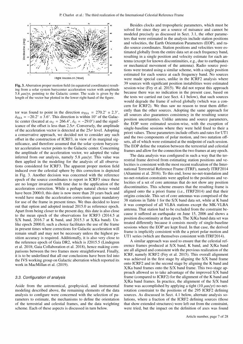
Fig. 3. Aberration proper motion field (in equatorial coordinates) result-ing from a solar system barycenter acceleration vector with amplitude5.8 µas/yr, pointing to the Galactic center. The scale is given by thelength of the vector bar plotted in the lower right-hand of the figure.
tor was found to point in the direction αSSA = 270.2◦ ± 2.3◦,δSSA = −20.2◦ ± 3.6◦. This direction is within 10◦ of the Galac-tic center (located at αG = 266.4◦, δG = −29.0◦) and the signif-icance of the offset is less than 2.5σ. Conversely, the amplitudeof the acceleration vector is detected at the 25σ level. Adoptinga conservative approach, we decided not to consider any suchoffset in the construction of ICRF3, in view of its marginal sig-nificance, and therefore assumed that the solar system barycen-ter acceleration vector points to the Galactic center. Concerningthe amplitude of the acceleration vector, we adopted the valueinferred from our analysis, namely 5.8 µas/yr. This value wasthen applied in the modeling for the analysis of all observa-tions considered for ICRF3. The apparent proper motion fieldinduced over the celestial sphere by this correction is depictedin Fig. 3. Another decision was concerned with the referenceepoch of the source coordinates to report in ICRF3 since theseare no longer invariant with time due to the application of theacceleration correction. While a perhaps natural choice wouldhave been 2000.0, this date is now more than 20 years back andwould have made the acceleration corrections quasi mandatoryfor use of the frame in present times. We thus decided to leaveout that option and adopted instead 2015.0 as reference epoch.Apart from being closer to the present day, this date is also closeto the mean epoch of the observations for ICRF3 (2014.5 atS/X band, 2016.7 at K band, and 2015.3 at X/Ka band). Un-like epoch 2000.0, such a choice facilitates the use of the framein present times where corrections for Galactic acceleration willremain small and may not be necessary unless the highest po-sition accuracy is required. Additionally, it is also very close tothe reference epoch of Gaia DR2, which is J2015.5 (Lindegrenet al. 2018; Gaia Collaboration et al. 2018), hence making com-parisons between the two frames more straightforward. Finally,it is to be underlined that all our conclusions have been fed intothe IVS working group on Galactic aberration which reported itswork in MacMillan et al. (2019).
3.3. Configuration of analysis
Aside from the astronomical, geophysical, and instrumentalmodeling described above, the remaining elements of the dataanalysis to configure were concerned with the selection of pa-rameters to estimate, the mechanisms to define the orientationof the terrestrial and celestial frames, and the data weightingscheme. Each of these aspects is discussed in turn below.
Besides clocks and tropospheric parameters, which must besolved for since they are a source of nuisance and cannot bemodeled precisely as discussed in Sect. 3.1, the other parame-ters that were estimated in the analysis include station positionsand velocities, the Earth Orientation Parameters (EOP), and ra-dio source coordinates. Station positions and velocities were es-timated globally from the entire data set at each frequency band,resulting in a single position and velocity estimate for each an-tenna (except for known discontinuities, e.g., due to earthquakesor mechanical movement of the antenna). Radio source posi-tions were treated using a similar scheme, with a single positionestimated for each source at each frequency band. No sourceswere made special cases, unlike in the ICRF2 analysis where39 sources with significant position instabilities were estimatedsession-wise (Fey et al. 2015). We did not repeat this approachbecause there was no indication in the present case, based onthe tests we carried out (see Sect. 4.1 below), that such sourceswould degrade the frame if solved globally (which was a con-cern for ICRF2). We thus saw no reason to treat them differ-ently than the other sources. Adopting the same approach forall sources also guarantees consistency in the resulting sourceposition uncertainties. Unlike antenna and source parameters,the EOP were estimated session-wise, with the exception ofsingle-baseline sessions where they were held fixed to their apriori values. Those parameters include offsets and rates for UT1and the two components of polar motion, and two nutation off-sets, all of which were estimated at the midpoint of each session.The EOP define the rotation between the terrestrial and celestialframes and allow for the connection the two frames at any epoch.
The data analysis was configured in such a way that the ter-restrial frame derived from estimating station positions and ve-locities is consistent with the most recent realization of the Inter-national Terrestrial Reference Frame (ITRF), namely ITRF2014(Altamimi et al. 2016). To this end, loose no-net-translation andno-net-rotation constraints were applied to the positions and ve-locities of a set of core antennas that do not show any positiondiscontinuities. This scheme ensures that the resulting frame isaligned onto the a priori frame (i.e., ITRF2014) and that theirorigins coincide. This set of core antennas was comprised of the38 stations in Table 1 for the S/X band data set, while at K bandit was comprised of all VLBA stations except the MK-VLBAantenna. That station had to be excluded from the constraint be-cause it suffered an earthquake on June 15, 2006 and shows aposition discontinuity at that epoch. The X/Ka band data set wastreated differently because it consists mostly of single-baselinesessions where the EOP are kept fixed. In that case, the derivedframe is implicitly consistent with the a priori polar motion andUT1 series (which are themselves consistent with ITRF2014).
A similar approach was used to ensure that the celestial ref-erence frames produced at S/X band, K band, and X/Ka bandare all aligned and consistent with the previous realization of theICRF, namely ICRF2 (Fey et al. 2015). This overall alignmentwas achieved in the first stage by aligning the S/X band frameonto ICRF2 and in the second stage by aligning the K band andX/Ka band frames onto the S/X band frame. This two-stage ap-proach allowed us to take advantage of the improved S/X bandframe (compared to ICRF2) for the alignment of the K band andX/Ka band frames. In practice, the alignment of the S/X bandframe was accomplished by applying a tight (10 µas/yr) no-net-rotation constraint to the positions of the 295 ICRF2 definingsources. As discussed in Sect. 4.1 below, alternate analysis so-lutions, where a fraction of the ICRF2 defining sources (thosethat show extended structures) were left out from the constraint,were tried, but the impact on the definition of axes was found
Article number, page 7 of 28
A&A proofs: manuscript no. icrf3
Table 1. Name, two-character code (as in Fig. 1), and geographical lo-cation of the 38 core antennas used to align the terrestrial referenceframe onto ITRF2014 in the S/X band analysis. The nine antennas withthe symbol † in superscript were also used for that alignment at K band.
Code Station name Longitude Latitude Location
Kk KOKEE −159.67 22.13 USAKu KAUAI −159.67 22.13 USAHc HATCREEK −121.47 40.82 USAVb VNDNBERG −120.62 34.56 USABr† BR-VLBA −119.68 48.13 USAOo OVRO_130 −118.28 37.23 USAOv† OV-VLBA −118.28 37.23 USAKp† KP-VLBA −111.61 31.96 USAPt† PIETOWN −108.12 34.30 USALa† LA-VLBA −106.25 35.78 USAFd† FD-VLBA −103.94 30.64 USANl† NL-VLBA −91.57 41.77 USARi RICHMOND −80.38 25.61 USAG3 NRAO85_3 −79.84 38.43 USAGn NRAO20 −79.83 38.44 USAAp ALGOPARK −78.07 45.96 CanadaHn† HN-VLBA −71.99 42.93 USAHs HAYSTACK −71.49 42.62 USAWf WESTFORD −71.49 42.61 USASt SANTIA12 −70.67 −33.15 ChileSc† SC-VLBA −64.58 17.76 USAFt FORTLEZA −38.43 −3.88 BrazilYs YEBES40M −3.09 40.52 SpainNy NYALES20 11.87 78.93 NorwayOn ONSALA60 11.93 57.40 SwedenWz WETTZELL 12.88 49.15 GermanyNt NOTO 14.99 36.88 ItalyMa MATERA 16.70 40.65 ItalyHh HARTRAO 27.69 −25.89 South AfricaSv SVETLOE 29.78 60.53 RussiaYg YARRA12M 115.35 −29.05 AustraliaSh SESHAN25 121.20 31.10 ChinaKe KATH12M 132.15 −14.38 AustraliaKa KASHIMA 140.66 35.95 JapanHb HOBART12 147.44 −42.80 AustraliaHo HOBART26 147.44 −42.80 Australia45 DSS45 148.98 −35.40 AustraliaWw WARK12M 174.83 −36.60 New Zealand
to be minimal. Therefore, we stuck to the original 295 ICRF2defining sources for fixing the orientation of the S/X band framethrough that constraint. As noted above, the S/X band frame,once realized, then served as a reference on which to align theK band and X/Ka band frames. To this end, a no-net-rotationconstraint was applied to the subset of ICRF3 defining sourcesincluded in the K band frame and the same was accomplished forthe X/Ka band frame (see Sect. 5.2 below for details on the se-lection of the ICRF3 defining sources). In all, there were 187 us-able ICRF3 defining sources at K band and 174 such sources atX/Ka band. At K band, six ICRF3 defining sources included inthe frame were deemed to be unsuitable for use in the rotationconstraints in this band because of too few (< 10) observations.In the case of X/Ka band, two ICRF3 defining sources includedin the frame (0346+800 and 0743−006) were also left out fromthe rotation constraints as possible outliers. The sources used toorient the K band and X/Ka frames are those labeled as definingsources in Tables 11 and 12 below with the above restrictions.
A final aspect of the analysis configuration is the weightingof the individual measurements. Following the usual VLBI prac-tice, the weighting factor wi assigned to a given observation i wasdetermined as a function of the unit weight σ0 as
wi =σ2
0
σ2i + σ2
s, (4)
whereσi is the formal uncertainty of that observation, derived onthe basis of the signal-to-noise ratio achieved from fringe-fittingand ionosphere calibration process (if applicable), and σs is abaseline-dependent additive noise calculated for each session.This additive noise was determined through an iterative proce-dure such that the reduced chi-squared4 of the post-fit residualson each baseline for each session is about unity. This schemeensures that the reduced chi-squared is close to unity over eachsession and furthermore over the entire data set as well.
3.4. Analysis software
An important element of the preparatory work for ICRF3 wasthat the data analysis was accomplished with several inde-pendent VLBI software packages running concurrently, one ofwhich was also run separately at three institutions. This allowedthe working group to check the results derived from these soft-ware packages against each other, which was essential to exposeany issues, and to gain confidence in the overall data analysisscheme while the work progressed, in particular through the gen-eration of several successive ICRF3 prototypes. Those softwarepackages are the following: CALC-SOLVE (Caprette et al. 1990,see appendix), MODEST (Sovers & Jacobs 1996), OCCAM(Titov et al. 2004), QUASAR (Kurdubov 2007), VieVS (Böhmet al. 2018), and VieVS@GFZ (Nilsson et al. 2015). A detaileddescription of these software packages is beyond the scope ofthis paper. In all, they use very similar modeling (as describedabove). However, they are based on different estimation meth-ods. CALC-SOLVE and VieVS use classical least-squares, whilethe other software packages employ specialized least-squaresor filtering methods – MODEST is based on the square-root-information filter, OCCAM and QUASAR on the least squarescollocation technique, and VieVS@GFZ on Kalman filtering.
While having such different software packages in hand wasof importance for the ICRF3 preparatory work, including numer-ous tests, the final ICRF3 product was derived from data pro-cessing with a unique software package at each frequency band.The S/X band and K band data sets were analyzed with CALC-SOLVE while the X/Ka band data set was analyzed with MOD-EST. Combination of results from different software packages,for example by combining the individual normal equations, wasinvestigated as an alternate option. However, it requires fine tun-ing of the input normal equations so that the estimated parame-ters are defined in a truly identical way in each software packageand have consistent a priori settings, which was not possible toachieve within the available time to produce ICRF3 due to soft-ware limitations and other issues. We thus decided to not followthat option and instead to prefer individual determinations.
The reason why the X/Ka band data set was processed witha different software package than the S/X band and K band datasets was mainly a matter of convenience due to the specificity of
4 The reduced chi-squared χ2ν is defined as χ2/ν where χ2 is the sum
of the squares of the weighted differences between the observed andcalculated quantities and ν is the degree of freedom which equals thenumber of observations minus the number of parameters.
Article number, page 8 of 28
P. Charlot et al.: The third realization of the International Celestial Reference Frame
the X/Ka band observations which are acquired, correlated, andpost-processed through an entirely separate path. The two soft-ware packages used in the final data analysis for ICRF3, CALC-SOLVE and MODEST, have been inter-compared, although notrecently, and were found to agree at the 1 ps level, as reportedin Ma et al. (1998). Therefore, we are confident that proceedingthis way does not limit the consistency of the ICRF3 results.
4. Assessment of errors
4.1. Variations in modeling and analysis configuration
An important part of the analysis work consisted in assessing theimpact of some of the key features adopted for ICRF3 in terms ofdata selection, modeling or analysis configuration. To this end,a number of alternate analysis solutions were carried out, eachof which varying a feature of interest. These alternate solutionswere then checked against our original analysis solution, in par-ticular by examining changes in the source positions, which al-lowed us to quantify the impact of those features on our results,including the level of systematic errors. All such tests were ac-complished based on the S/X band data set and employed theCALC-SOLVE software package to guarantee the consistencyof those alternate solutions with our original analysis solution.
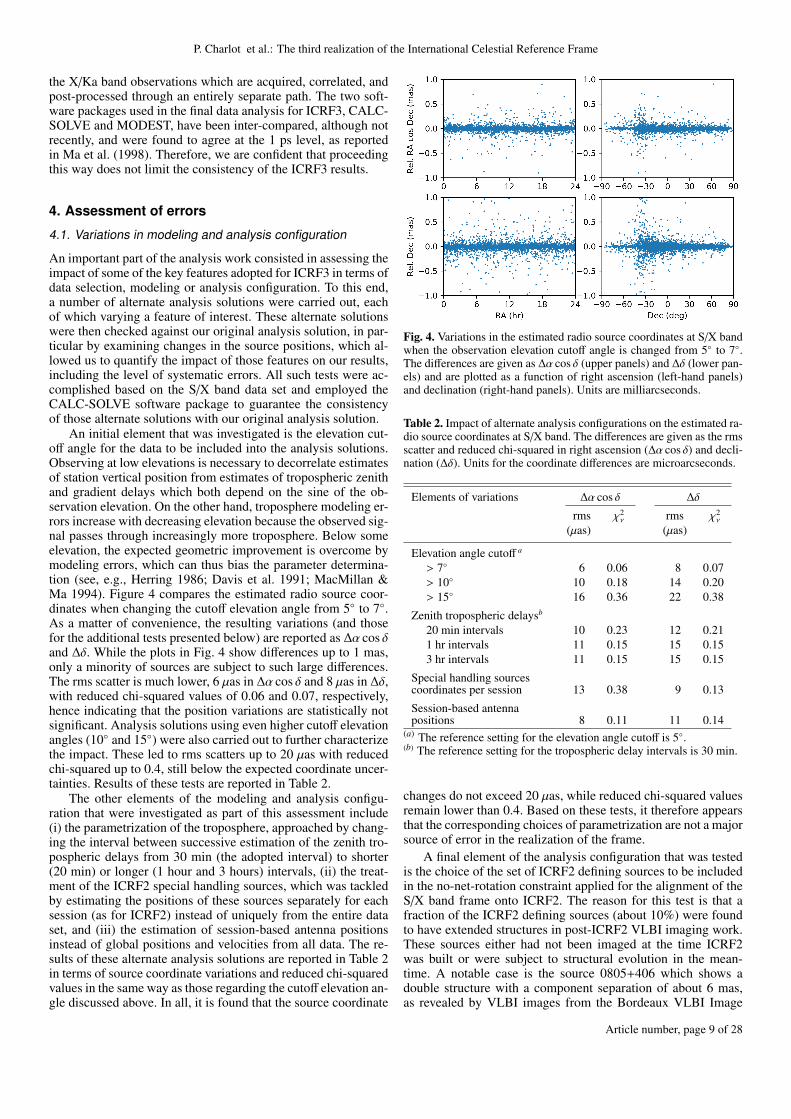
An initial element that was investigated is the elevation cut-off angle for the data to be included into the analysis solutions.Observing at low elevations is necessary to decorrelate estimatesof station vertical position from estimates of tropospheric zenithand gradient delays which both depend on the sine of the ob-servation elevation. On the other hand, troposphere modeling er-rors increase with decreasing elevation because the observed sig-nal passes through increasingly more troposphere. Below someelevation, the expected geometric improvement is overcome bymodeling errors, which can thus bias the parameter determina-tion (see, e.g., Herring 1986; Davis et al. 1991; MacMillan &Ma 1994). Figure 4 compares the estimated radio source coor-dinates when changing the cutoff elevation angle from 5◦ to 7◦.As a matter of convenience, the resulting variations (and thosefor the additional tests presented below) are reported as ∆α cos δand ∆δ. While the plots in Fig. 4 show differences up to 1 mas,only a minority of sources are subject to such large differences.The rms scatter is much lower, 6 µas in ∆α cos δ and 8 µas in ∆δ,with reduced chi-squared values of 0.06 and 0.07, respectively,hence indicating that the position variations are statistically notsignificant. Analysis solutions using even higher cutoff elevationangles (10◦ and 15◦) were also carried out to further characterizethe impact. These led to rms scatters up to 20 µas with reducedchi-squared up to 0.4, still below the expected coordinate uncer-tainties. Results of these tests are reported in Table 2.
The other elements of the modeling and analysis configu-ration that were investigated as part of this assessment include(i) the parametrization of the troposphere, approached by chang-ing the interval between successive estimation of the zenith tro-pospheric delays from 30 min (the adopted interval) to shorter(20 min) or longer (1 hour and 3 hours) intervals, (ii) the treat-ment of the ICRF2 special handling sources, which was tackledby estimating the positions of these sources separately for eachsession (as for ICRF2) instead of uniquely from the entire dataset, and (iii) the estimation of session-based antenna positionsinstead of global positions and velocities from all data. The re-sults of these alternate analysis solutions are reported in Table 2in terms of source coordinate variations and reduced chi-squaredvalues in the same way as those regarding the cutoff elevation an-gle discussed above. In all, it is found that the source coordinate
Fig. 4. Variations in the estimated radio source coordinates at S/X bandwhen the observation elevation cutoff angle is changed from 5◦ to 7◦.The differences are given as ∆α cos δ (upper panels) and ∆δ (lower pan-els) and are plotted as a function of right ascension (left-hand panels)and declination (right-hand panels). Units are milliarcseconds.
Table 2. Impact of alternate analysis configurations on the estimated ra-dio source coordinates at S/X band. The differences are given as the rmsscatter and reduced chi-squared in right ascension (∆α cos δ) and decli-nation (∆δ). Units for the coordinate differences are microarcseconds.
Elements of variations ∆α cos δ ∆δ
rms χ2ν rms χ2
ν
(µas) (µas)
Elevation angle cutoff a
> 7◦ 6 0.06 8 0.07> 10◦ 10 0.18 14 0.20> 15◦ 16 0.36 22 0.38
Zenith tropospheric delaysb
20 min intervals 10 0.23 12 0.211 hr intervals 11 0.15 15 0.153 hr intervals 11 0.15 15 0.15
Special handling sourcescoordinates per session 13 0.38 9 0.13
Session-based antennapositions 8 0.11 11 0.14
(a) The reference setting for the elevation angle cutoff is 5◦.(b) The reference setting for the tropospheric delay intervals is 30 min.
changes do not exceed 20 µas, while reduced chi-squared valuesremain lower than 0.4. Based on these tests, it therefore appearsthat the corresponding choices of parametrization are not a majorsource of error in the realization of the frame.
A final element of the analysis configuration that was testedis the choice of the set of ICRF2 defining sources to be includedin the no-net-rotation constraint applied for the alignment of theS/X band frame onto ICRF2. The reason for this test is that afraction of the ICRF2 defining sources (about 10%) were foundto have extended structures in post-ICRF2 VLBI imaging work.These sources either had not been imaged at the time ICRF2was built or were subject to structural evolution in the mean-time. A notable case is the source 0805+406 which shows adouble structure with a component separation of about 6 mas,as revealed by VLBI images from the Bordeaux VLBI Image
Article number, page 9 of 28
A&A proofs: manuscript no. icrf3
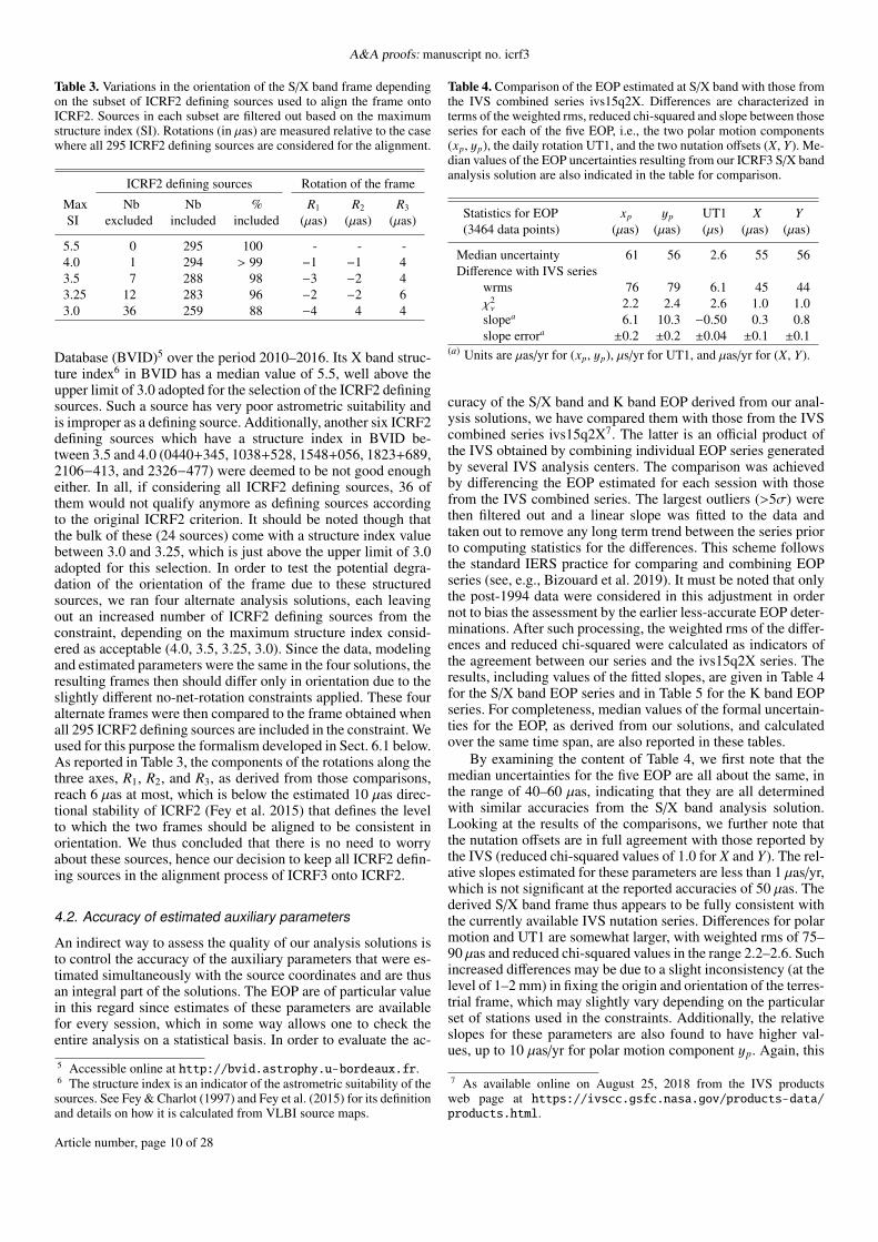
Table 3. Variations in the orientation of the S/X band frame dependingon the subset of ICRF2 defining sources used to align the frame ontoICRF2. Sources in each subset are filtered out based on the maximumstructure index (SI). Rotations (in µas) are measured relative to the casewhere all 295 ICRF2 defining sources are considered for the alignment.
ICRF2 defining sources Rotation of the frame
Max Nb Nb % R1 R2 R3
SI excluded included included (µas) (µas) (µas)
5.5 0 295 100 - - -4.0 1 294 > 99 −1 −1 43.5 7 288 98 −3 −2 43.25 12 283 96 −2 −2 63.0 36 259 88 −4 4 4
Database (BVID)5 over the period 2010–2016. Its X band struc-ture index6 in BVID has a median value of 5.5, well above theupper limit of 3.0 adopted for the selection of the ICRF2 definingsources. Such a source has very poor astrometric suitability andis improper as a defining source. Additionally, another six ICRF2defining sources which have a structure index in BVID be-tween 3.5 and 4.0 (0440+345, 1038+528, 1548+056, 1823+689,2106−413, and 2326−477) were deemed to be not good enougheither. In all, if considering all ICRF2 defining sources, 36 ofthem would not qualify anymore as defining sources accordingto the original ICRF2 criterion. It should be noted though thatthe bulk of these (24 sources) come with a structure index valuebetween 3.0 and 3.25, which is just above the upper limit of 3.0adopted for this selection. In order to test the potential degra-dation of the orientation of the frame due to these structuredsources, we ran four alternate analysis solutions, each leavingout an increased number of ICRF2 defining sources from theconstraint, depending on the maximum structure index consid-ered as acceptable (4.0, 3.5, 3.25, 3.0). Since the data, modelingand estimated parameters were the same in the four solutions, theresulting frames then should differ only in orientation due to theslightly different no-net-rotation constraints applied. These fouralternate frames were then compared to the frame obtained whenall 295 ICRF2 defining sources are included in the constraint. Weused for this purpose the formalism developed in Sect. 6.1 below.As reported in Table 3, the components of the rotations along thethree axes, R1, R2, and R3, as derived from those comparisons,reach 6 µas at most, which is below the estimated 10 µas direc-tional stability of ICRF2 (Fey et al. 2015) that defines the levelto which the two frames should be aligned to be consistent inorientation. We thus concluded that there is no need to worryabout these sources, hence our decision to keep all ICRF2 defin-ing sources in the alignment process of ICRF3 onto ICRF2.
4.2. Accuracy of estimated auxiliary parameters
An indirect way to assess the quality of our analysis solutions isto control the accuracy of the auxiliary parameters that were es-timated simultaneously with the source coordinates and are thusan integral part of the solutions. The EOP are of particular valuein this regard since estimates of these parameters are availablefor every session, which in some way allows one to check theentire analysis on a statistical basis. In order to evaluate the ac-
5 Accessible online at http://bvid.astrophy.u-bordeaux.fr.6 The structure index is an indicator of the astrometric suitability of thesources. See Fey & Charlot (1997) and Fey et al. (2015) for its definitionand details on how it is calculated from VLBI source maps.
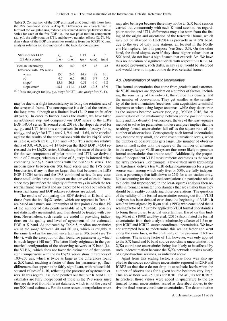
Table 4. Comparison of the EOP estimated at S/X band with those fromthe IVS combined series ivs15q2X. Differences are characterized interms of the weighted rms, reduced chi-squared and slope between thoseseries for each of the five EOP, i.e., the two polar motion components(xp, yp), the daily rotation UT1, and the two nutation offsets (X, Y). Me-dian values of the EOP uncertainties resulting from our ICRF3 S/X bandanalysis solution are also indicated in the table for comparison.
Statistics for EOP xp yp UT1 X Y(3464 data points) (µas) (µas) (µs) (µas) (µas)
Median uncertainty 61 56 2.6 55 56Difference with IVS series
wrms 76 79 6.1 45 44χ2ν 2.2 2.4 2.6 1.0 1.0
slopea 6.1 10.3 −0.50 0.3 0.8slope errora ±0.2 ±0.2 ±0.04 ±0.1 ±0.1
(a) Units are µas/yr for (xp, yp), µs/yr for UT1, and µas/yr for (X, Y).
curacy of the S/X band and K band EOP derived from our anal-ysis solutions, we have compared them with those from the IVScombined series ivs15q2X7. The latter is an official product ofthe IVS obtained by combining individual EOP series generatedby several IVS analysis centers. The comparison was achievedby differencing the EOP estimated for each session with thosefrom the IVS combined series. The largest outliers (>5σ) werethen filtered out and a linear slope was fitted to the data andtaken out to remove any long term trend between the series priorto computing statistics for the differences. This scheme followsthe standard IERS practice for comparing and combining EOPseries (see, e.g., Bizouard et al. 2019). It must be noted that onlythe post-1994 data were considered in this adjustment in ordernot to bias the assessment by the earlier less-accurate EOP deter-minations. After such processing, the weighted rms of the differ-ences and reduced chi-squared were calculated as indicators ofthe agreement between our series and the ivs15q2X series. Theresults, including values of the fitted slopes, are given in Table 4for the S/X band EOP series and in Table 5 for the K band EOPseries. For completeness, median values of the formal uncertain-ties for the EOP, as derived from our solutions, and calculatedover the same time span, are also reported in these tables.
By examining the content of Table 4, we first note that themedian uncertainties for the five EOP are all about the same, inthe range of 40–60 µas, indicating that they are all determinedwith similar accuracies from the S/X band analysis solution.Looking at the results of the comparisons, we further note thatthe nutation offsets are in full agreement with those reported bythe IVS (reduced chi-squared values of 1.0 for X and Y). The rel-ative slopes estimated for these parameters are less than 1 µas/yr,which is not significant at the reported accuracies of 50 µas. Thederived S/X band frame thus appears to be fully consistent withthe currently available IVS nutation series. Differences for polarmotion and UT1 are somewhat larger, with weighted rms of 75–90 µas and reduced chi-squared values in the range 2.2–2.6. Suchincreased differences may be due to a slight inconsistency (at thelevel of 1–2 mm) in fixing the origin and orientation of the terres-trial frame, which may slightly vary depending on the particularset of stations used in the constraints. Additionally, the relativeslopes for these parameters are also found to have higher val-ues, up to 10 µas/yr for polar motion component yp. Again, this
7 As available online on August 25, 2018 from the IVS productsweb page at https://ivscc.gsfc.nasa.gov/products-data/products.html.
Article number, page 10 of 28
P. Charlot et al.: The third realization of the International Celestial Reference Frame
Table 5. Comparison of the EOP estimated at K band with those fromthe IVS combined series ivs15q2X. Differences are characterized interms of the weighted rms, reduced chi-squared and slope between thoseseries for each of the five EOP, i.e., the two polar motion components(xp, yp), the daily rotation UT1, and the two nutation offsets (X, Y). Me-dian values of the EOP uncertainties resulting from our ICRF3 K bandanalysis solution are also indicated in the table for comparison.
Statistics for EOP xp yp UT1 X Y(27 data points) (µas) (µas) (µs) (µas) (µas)
Median uncertainty 66 140 5.5 43 42Difference with IVS series
wrms 153 246 14.9 88 101χ2ν 4.7 6.5 10.2 3.7 5.5
slopea 15.6 20.1 0.51 −1.0 −6.8slope errora ±8.1 ±11.4 ±1.65 ±3.5 ±3.9
(a) Units are µas/yr for (xp, yp), µs/yr for UT1, and µas/yr for (X, Y).
may be due to a slight inconsistency in fixing the rotation rate ofthe terrestrial frame. The consequence is a drift of the series onthe long term, although at a limited level (7–12 mm shifts after40 years). In order to further assess the matter, we have takenan additional step and compared our EOP series to the IERSEOP 14C04 series (Bizouard et al. 2019). The slopes derived forxp, yp, and UT1 from this comparison (in units of µas/yr for xpand yp, and µs/yr for UT1) are 9.1, 9.4, and −1.64, to be checkedagainst the results of the comparisons with the ivs15q2X seriesin Table 4, which are 6.1, 10.3, and −0.50. This indicates relativedrifts of 3.0, −0.9, and −1.14 between the IERS EOP 14C04 se-ries and the ivs15q2X series. Calculating the mean of these driftsfor the two components of polar motion and UT1, we derive avalue of 7 µas/yr, whereas a value of 8 µas/yr is inferred whencomparing our S/X band series with the ivs15q2X series. Theinconsistency between our S/X band series and the IVS com-bined series, if any, is thus no larger than that between the IERSEOP 14C04 series and the IVS combined series. In any case,those small drifts have no impact on the derived celestial framesince they just reflect the slightly different ways in which the ter-restrial frame was fixed and are expected to cancel out when theterrestrial frame and EOP relative rotations are added.
The results of comparing the EOP derived at K band withthose from the ivs15q2X series, which are reported in Table 5,are based on a much smaller number of data points (less than 1%of the number of data points available at S/X band), possiblynot statistically meaningful, and thus should be treated with cau-tion. Nevertheless, such results are useful in providing indica-tions on the quality and level of agreement of the estimatedEOP at K band. As indicated by Table 5, median uncertaintiesare in the range between 40 and 80 µas, which is roughly atthe same level as the median uncertainties at S/X band (see Ta-ble 4), with the exception of that found for parameter yp whichis much larger (140 µas). The latter likely originates in the geo-metrical configuration of the observing network at K band (i.e.,the VLBA), which does not favor the estimation of that param-eter. Comparisons with the ivs15q2X series show differences of100–250 µas, which is twice as large as the differences foundat S/X band, reaching a factor of three for parameter yp. Suchdifferences also appear to be fairly significant, with reduced chi-squared values of 4–10, reflecting the presence of systematic er-rors. In this regard, it is to be pointed out that our K band EOPestimates are fully independent of those in the IVS series sincethey are derived from different data sets, which is not the case ofour S/X band estimates. For the same reason, interpolation errors
may also be larger because there may not be an S/X band sessioncarried out concurrently with each K band session. As regardspolar motion and UT1, differences may also stem from the fix-ing of the origin and orientation of the terrestrial frame, whichmay not be attached to ITRF2014 as precisely as at S/X band,due to the use of only nine stations, all located in the North-ern Hemisphere, for this purpose (see Sect. 3.3). On the otherhand, the fitted slopes, even if they show higher values than atS/X band, do not have a significance that exceeds 2σ. We havethus no indication of significant drifts with respect to ITRF2014.As noted previously, such drifts, in any case, would be absorbedand would have no impact on the derived celestial frame.
4.3. Determination of realistic uncertainties
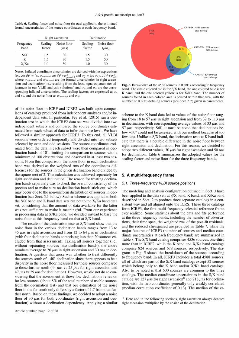
The formal uncertainties that come from geodetic and astromet-ric VLBI analyses are dependent on a number of factors, includ-ing the sensitivity of the network, the source flux density, andthe number of observations. They get smaller as the sensitiv-ity of the instrumentation (receivers, data acquisition terminals)improves or when using larger antennas, while they deteriorateas the sources become weaker (see, e.g., Malkin 2016, for aninvestigation of the relationship between source position uncer-tainty and flux density). Furthermore, the use of the least-squaresmethod to solve for parameters in these analyses implies that theresulting formal uncertainties fall off as the square root of thenumber of observations. Consequently, such formal uncertaintiesmay become very small, and even reach unrealistic levels, whenthe number of observations gets large. The number of observa-tions in itself scales with the square of the number of antennasin the array. Larger VLBI arrays are thus more likely to generateformal uncertainties that are too small. Additionally, the propor-tion of independent VLBI measurements decreases as the size ofthe array increases. For example, a five-station array (providingten baselines) delivers ten VLBI delay measurements for a givensource scan, among which only five, or 50%, are fully indepen-dent, a percentage that falls down to 22% for a ten-station array.Not accounting for the induced correlations (in particular relatedto clocks and troposphere) in the least-squares analysis then re-sults in formal parameter uncertainties that are smaller than theyshould be in reality considering those correlations. The questionof the validity of the formal uncertainties coming out from VLBIanalyses has been debated ever since the beginning of VLBI. Itwas first investigated by Ryan et al. (1993) who concluded that ascaling factor of 1.5 is to be applied to VLBI formal uncertaintiesto bring them closer to actual uncertainties. Based on this find-ing, Ma et al. (1998) and Fey et al. (2015) also inflated the formaluncertainties from their analysis solutions by a factor of 1.5 to re-port ICRF and ICRF2 source coordinate uncertainties. We havenot attempted here to redetermine this scaling factor and wentalong the same lines, in the continuity of the previous ICRF re-alizations. The scaling factor of 1.5, however, was only appliedto the S/X band and K band source coordinate uncertainties, theX/Ka coordinate uncertainties being less likely to be affected bysuch underestimation because the X/Ka network consists mostlyof single-baseline sessions, as indicated above.
Apart from this scaling factor, a noise floor was also ap-plied to the source coordinate uncertainties reported in ICRF andICRF2 so that these do not drop to unrealistic levels when thenumber of observations for a given source becomes very large.This noise floor was 250 µas for ICRF and 40 µas for ICRF2.In practice, those values were added in quadrature to the es-timated formal uncertainties, scaled as described above, to de-rive the final source coordinate uncertainties. The determination
Article number, page 11 of 28
A&A proofs: manuscript no. icrf3
Table 6. Scaling factor and noise floor (in µas) applied to the estimatedformal uncertainties of the source coordinates at each frequency band.
Right ascension Declination
Frequency Scaling Noise floor Scaling Noise floorband factor (µas) factor (µas)
S/X 1.5 30 1.5 30K 1.5 30 1.5 50
X/Ka 1.0 30 1.0 30
Notes. Inflated coordinate uncertainties are derived with the expressions(σα cos δ)2 = (sα σα,formal cos δ)2 +σ2
α cos δ,0 and σ2δ = (sδ σδ,formal)2 +σ2
δ,0,where σα,formal and σδ,formal are the formal uncertainties in right ascen-sion and declination (i.e., resulting from the least-squares parameter ad-justment in our VLBI analysis solutions) and σα and σδ are the corre-sponding inflated uncertainties. The scaling factors are expressed as sαand sδ, and the noise floor as σα cos δ,0 and σδ,0.
of the noise floor in ICRF and ICRF2 was built upon compar-isons of catalogs produced from independent analyses and/or in-dependent data sets. In particular, Fey et al. (2015) ran a dec-imation test in which the ICRF2 data set was divided into twoindependent subsets and compared the source coordinates esti-mated from each subset of data to infer the noise level. We havefollowed a similar approach for ICRF3. To this end, all VLBIsessions were ordered temporally and divided into two subsetsselected by even and odd sessions. The source coordinates esti-mated from the data in each subset were then compared in dec-lination bands of 10◦, limiting the comparison to sources with aminimum of 100 observations and observed in at least two ses-sions. From this comparison, the noise floor in each declinationband was derived as the weighted rms of the coordinates dif-ferences for the sources in the given declination band divided bythe square root of 2. That calculation was achieved separately forright ascension and declination. The reason for treating declina-tion bands separately was to check the overall consistency of theprocess and to make sure no declination bands stick out, whichmay occur due to the non-uniform distribution of sources in dec-lination (see Sect. 5.1 below). Such a scheme was applied to boththe S/X band and K band data sets but not to the X/Ka band dataset, considering that the amount of data available for the latterwas not sufficient to make it meaningful. From our experiencein processing data at X/Ka band, we decided instead to base thenoise floor at this frequency band on that at S/X band.
The results of the decimation tests at S/X band show that thenoise floor in the various declination bands ranges from 13 to45 µas in right ascension and from 12 to 64 µas in declination(with four declination bands comprising less than 20 sources ex-cluded from that assessment). Taking all sources together (i.e.,without separating sources into declination bands), the abovenumbers average to 26 µas in right ascension and 30 µas in dec-lination. A question that arose was whether to treat differentlythe sources south of −40◦ declination since there appears to be adisparity in the noise floor measured for these sources comparedto those further north (44 µas vs 25 µas for right ascension and47 µas vs 29 µas for declination). However, we did not do so con-sidering that the assessment at those low declinations relies onfar less sources (about 8% of the total number of usable sourcesfrom the decimation test) and that our estimation of the noisefloor in the far south only differs by a factor of 1.7 from that fur-ther north. Based on these findings, we decided to adopt a noisefloor of 30 µas for both coordinates (right ascension and dec-lination) without a declination dependency. Applying a similar
3705(105)
ICRF3-SX : 4536 sources(303 defining)
ICRF3-XKa : 678 sources(176 defining)
ICRF3-K : 824 sources(193 defining)
38 (5)
21600(171)
19
12
193(22)
Fig. 5. Breakdown of the 4588 sources in ICRF3 according to frequencyband. The circle colored red is for S/X band, the one colored blue is forK band, and the one colored yellow is for X/Ka band. The number ofsources found in each colored area is printed within that area, with thenumber of ICRF3 defining sources (see Sect. 5.2) given in parentheses.
scheme to the K band data led to values of the noise floor rang-ing from 18 to 57 µas in right ascension and from 32 to 113 µasin declination, with corresponding average values of 33 µas and57 µas, respectively. Still, it must be noted that declinations be-low −30◦ could not be assessed with our method because of toofew data. Unlike at S/X band, the decimation tests at K band indi-cate that there is a notable difference in the noise floor betweenright ascension and declination. For this reason, we decided toadopt two different values, 30 µas for right ascension and 50 µasfor declination. Table 6 summarizes the adopted values for thescaling factor and noise floor for the three frequency bands.
5. A multi-frequency frame
5.1. Three-frequency VLBI source positions
The modeling and analysis configuration outlined in Sect. 3 havebeen applied to the data sets at S/X band, K band, and X/Ka banddescribed in Sect. 2 to produce three separate catalogs in a con-sistent way and all aligned onto the ICRS. These three catalogsform ICRF3, the first multi-frequency celestial reference frameever realized. Some statistics about the data and fits performedat the three frequency bands, including the number of observa-tions, their time span, the weighted rms of the post-fit residuals,and the reduced chi-squared are provided in Table 7, while themajor features of ICRF3 (number of sources and median coor-dinate uncertainties at each frequency band) are summarized inTable 8. The S/X band catalog comprises 4536 sources, one-thirdmore than in ICRF2, while the K band and X/Ka band catalogscomprise 824 sources and 678 sources, respectively. The dia-gram in Fig. 5 shows the breakdown of the sources accordingto frequency band. In all, ICRF3 includes a total 4588 sources,all of which are part of the S/X band catalog, except 52 sourceswhich belong only to the K band and/or X/Ka band catalogs.Also to be noted is that 600 sources are common to the threecatalogs. The median coordinate uncertainties in the S/X bandcatalog are 127 µas for right ascension8 and 218 µas for declina-tion, with the two coordinates generally only weakly correlated(median correlation coefficient of 0.13). The median of the er-
8 Here and in the following sections, right ascension always denotesright ascension multiplied by the cosine of the declination.
Article number, page 12 of 28
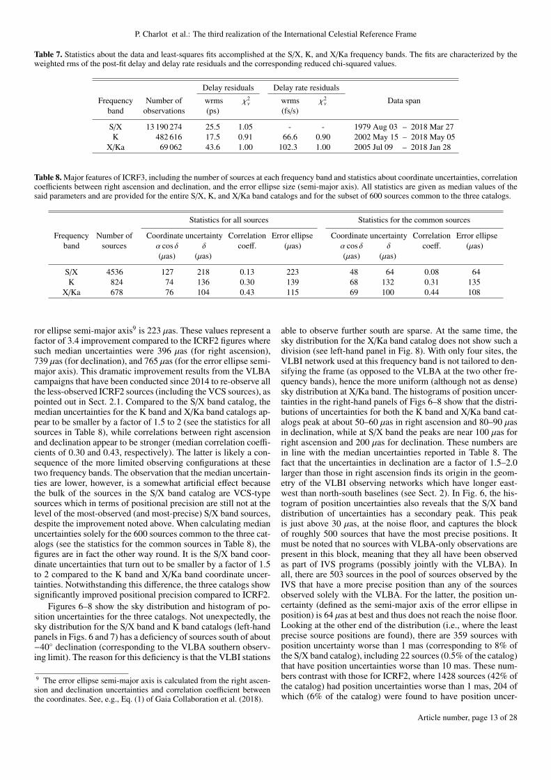
P. Charlot et al.: The third realization of the International Celestial Reference Frame
Table 7. Statistics about the data and least-squares fits accomplished at the S/X, K, and X/Ka frequency bands. The fits are characterized by theweighted rms of the post-fit delay and delay rate residuals and the corresponding reduced chi-squared values.
Delay residuals Delay rate residuals
Frequency Number of wrms χ2ν wrms χ2
ν Data spanband observations (ps) (fs/s)
S/X 13 190 274 25.5 1.05 - - 1979 Aug 03 – 2018 Mar 27K 482 616 17.5 0.91 66.6 0.90 2002 May 15 – 2018 May 05
X/Ka 69 062 43.6 1.00 102.3 1.00 2005 Jul 09 – 2018 Jan 28
Table 8. Major features of ICRF3, including the number of sources at each frequency band and statistics about coordinate uncertainties, correlationcoefficients between right ascension and declination, and the error ellipse size (semi-major axis). All statistics are given as median values of thesaid parameters and are provided for the entire S/X, K, and X/Ka band catalogs and for the subset of 600 sources common to the three catalogs.
Statistics for all sources Statistics for the common sources
Frequency Number of Coordinate uncertainty Correlation Error ellipse Coordinate uncertainty Correlation Error ellipseband sources α cos δ δ coeff. (µas) α cos δ δ coeff. (µas)
(µas) (µas) (µas) (µas)
S/X 4536 127 218 0.13 223 48 64 0.08 64K 824 74 136 0.30 139 68 132 0.31 135
X/Ka 678 76 104 0.43 115 69 100 0.44 108
ror ellipse semi-major axis9 is 223 µas. These values represent afactor of 3.4 improvement compared to the ICRF2 figures wheresuch median uncertainties were 396 µas (for right ascension),739 µas (for declination), and 765 µas (for the error ellipse semi-major axis). This dramatic improvement results from the VLBAcampaigns that have been conducted since 2014 to re-observe allthe less-observed ICRF2 sources (including the VCS sources), aspointed out in Sect. 2.1. Compared to the S/X band catalog, themedian uncertainties for the K band and X/Ka band catalogs ap-pear to be smaller by a factor of 1.5 to 2 (see the statistics for allsources in Table 8), while correlations between right ascensionand declination appear to be stronger (median correlation coeffi-cients of 0.30 and 0.43, respectively). The latter is likely a con-sequence of the more limited observing configurations at thesetwo frequency bands. The observation that the median uncertain-ties are lower, however, is a somewhat artificial effect becausethe bulk of the sources in the S/X band catalog are VCS-typesources which in terms of positional precision are still not at thelevel of the most-observed (and most-precise) S/X band sources,despite the improvement noted above. When calculating medianuncertainties solely for the 600 sources common to the three cat-alogs (see the statistics for the common sources in Table 8), thefigures are in fact the other way round. It is the S/X band coor-dinate uncertainties that turn out to be smaller by a factor of 1.5to 2 compared to the K band and X/Ka band coordinate uncer-tainties. Notwithstanding this difference, the three catalogs showsignificantly improved positional precision compared to ICRF2.
Figures 6–8 show the sky distribution and histogram of po-sition uncertainties for the three catalogs. Not unexpectedly, thesky distribution for the S/X band and K band catalogs (left-handpanels in Figs. 6 and 7) has a deficiency of sources south of about−40◦ declination (corresponding to the VLBA southern observ-ing limit). The reason for this deficiency is that the VLBI stations
9 The error ellipse semi-major axis is calculated from the right ascen-sion and declination uncertainties and correlation coefficient betweenthe coordinates. See, e.g., Eq. (1) of Gaia Collaboration et al. (2018).
able to observe further south are sparse. At the same time, thesky distribution for the X/Ka band catalog does not show such adivision (see left-hand panel in Fig. 8). With only four sites, theVLBI network used at this frequency band is not tailored to den-sifying the frame (as opposed to the VLBA at the two other fre-quency bands), hence the more uniform (although not as dense)sky distribution at X/Ka band. The histograms of position uncer-tainties in the right-hand panels of Figs 6–8 show that the distri-butions of uncertainties for both the K band and X/Ka band cat-alogs peak at about 50–60 µas in right ascension and 80–90 µasin declination, while at S/X band the peaks are near 100 µas forright ascension and 200 µas for declination. These numbers arein line with the median uncertainties reported in Table 8. Thefact that the uncertainties in declination are a factor of 1.5–2.0larger than those in right ascension finds its origin in the geom-etry of the VLBI observing networks which have longer east-west than north-south baselines (see Sect. 2). In Fig. 6, the his-togram of position uncertainties also reveals that the S/X banddistribution of uncertainties has a secondary peak. This peakis just above 30 µas, at the noise floor, and captures the blockof roughly 500 sources that have the most precise positions. Itmust be noted that no sources with VLBA-only observations arepresent in this block, meaning that they all have been observedas part of IVS programs (possibly jointly with the VLBA). Inall, there are 503 sources in the pool of sources observed by theIVS that have a more precise position than any of the sourcesobserved solely with the VLBA. For the latter, the position un-certainty (defined as the semi-major axis of the error ellipse inposition) is 64 µas at best and thus does not reach the noise floor.Looking at the other end of the distribution (i.e., where the leastprecise source positions are found), there are 359 sources withposition uncertainty worse than 1 mas (corresponding to 8% ofthe S/X band catalog), including 22 sources (0.5% of the catalog)that have position uncertainties worse than 10 mas. These num-bers contrast with those for ICRF2, where 1428 sources (42% ofthe catalog) had position uncertainties worse than 1 mas, 204 ofwhich (6% of the catalog) were found to have position uncer-
Article number, page 13 of 28
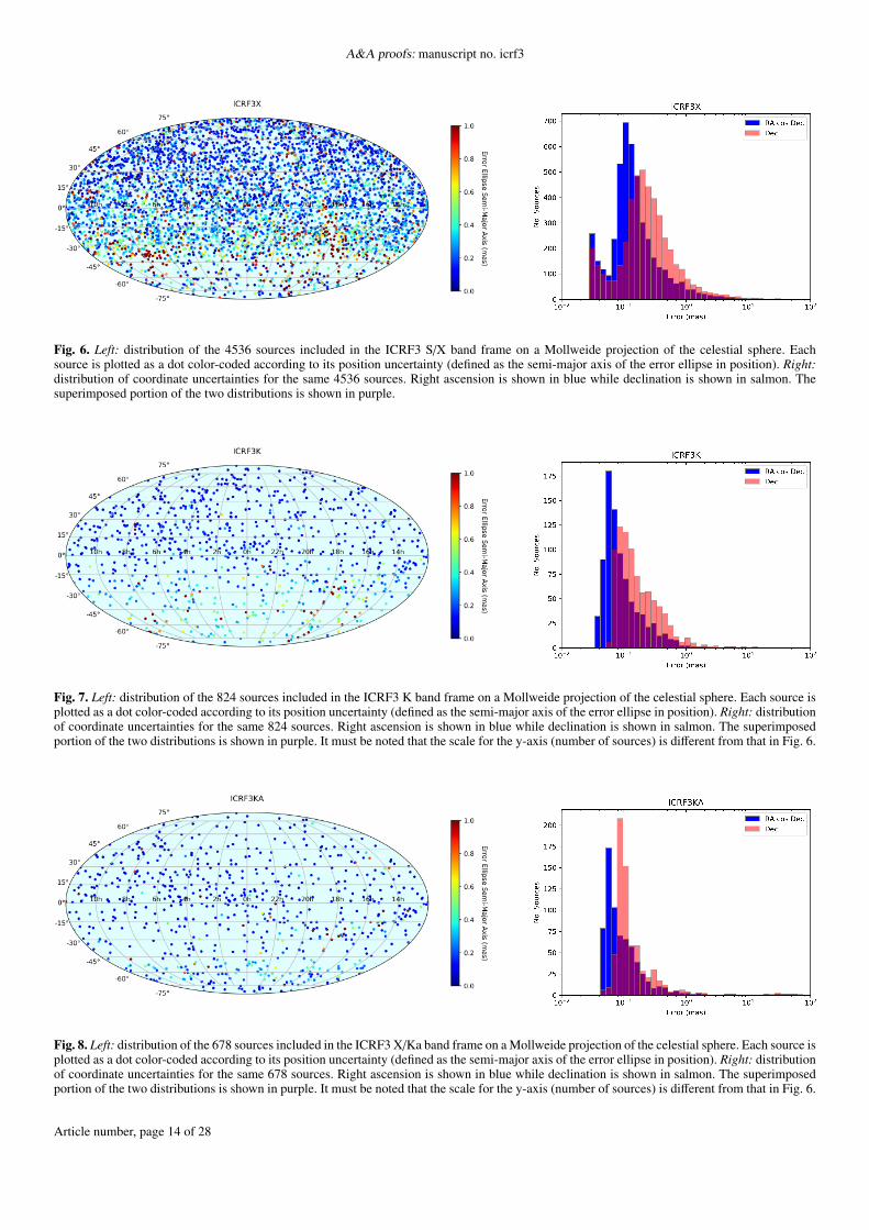
A&A proofs: manuscript no. icrf3
Fig. 6. Left: distribution of the 4536 sources included in the ICRF3 S/X band frame on a Mollweide projection of the celestial sphere. Eachsource is plotted as a dot color-coded according to its position uncertainty (defined as the semi-major axis of the error ellipse in position). Right:distribution of coordinate uncertainties for the same 4536 sources. Right ascension is shown in blue while declination is shown in salmon. Thesuperimposed portion of the two distributions is shown in purple.
Fig. 7. Left: distribution of the 824 sources included in the ICRF3 K band frame on a Mollweide projection of the celestial sphere. Each source isplotted as a dot color-coded according to its position uncertainty (defined as the semi-major axis of the error ellipse in position). Right: distributionof coordinate uncertainties for the same 824 sources. Right ascension is shown in blue while declination is shown in salmon. The superimposedportion of the two distributions is shown in purple. It must be noted that the scale for the y-axis (number of sources) is different from that in Fig. 6.
Fig. 8. Left: distribution of the 678 sources included in the ICRF3 X/Ka band frame on a Mollweide projection of the celestial sphere. Each source isplotted as a dot color-coded according to its position uncertainty (defined as the semi-major axis of the error ellipse in position). Right: distributionof coordinate uncertainties for the same 678 sources. Right ascension is shown in blue while declination is shown in salmon. The superimposedportion of the two distributions is shown in purple. It must be noted that the scale for the y-axis (number of sources) is different from that in Fig. 6.
Article number, page 14 of 28
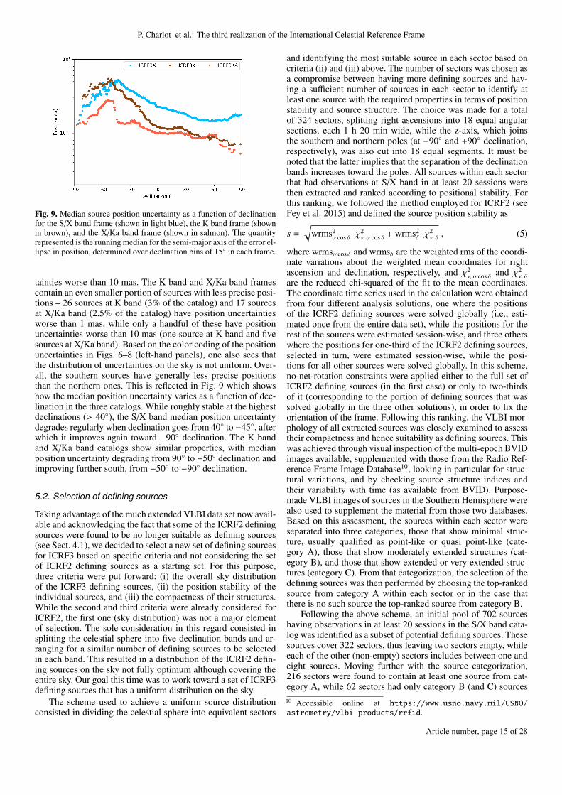
P. Charlot et al.: The third realization of the International Celestial Reference Frame
Fig. 9. Median source position uncertainty as a function of declinationfor the S/X band frame (shown in light blue), the K band frame (shownin brown), and the X/Ka band frame (shown in salmon). The quantityrepresented is the running median for the semi-major axis of the error el-lipse in position, determined over declination bins of 15◦ in each frame.
tainties worse than 10 mas. The K band and X/Ka band framescontain an even smaller portion of sources with less precise posi-tions – 26 sources at K band (3% of the catalog) and 17 sourcesat X/Ka band (2.5% of the catalog) have position uncertaintiesworse than 1 mas, while only a handful of these have positionuncertainties worse than 10 mas (one source at K band and fivesources at X/Ka band). Based on the color coding of the positionuncertainties in Figs. 6–8 (left-hand panels), one also sees thatthe distribution of uncertainties on the sky is not uniform. Over-all, the southern sources have generally less precise positionsthan the northern ones. This is reflected in Fig. 9 which showshow the median position uncertainty varies as a function of dec-lination in the three catalogs. While roughly stable at the highestdeclinations (> 40◦), the S/X band median position uncertaintydegrades regularly when declination goes from 40◦ to −45◦, afterwhich it improves again toward −90◦ declination. The K bandand X/Ka band catalogs show similar properties, with medianposition uncertainty degrading from 90◦ to −50◦ declination andimproving further south, from −50◦ to −90◦ declination.
5.2. Selection of defining sources
Taking advantage of the much extended VLBI data set now avail-able and acknowledging the fact that some of the ICRF2 definingsources were found to be no longer suitable as defining sources(see Sect. 4.1), we decided to select a new set of defining sourcesfor ICRF3 based on specific criteria and not considering the setof ICRF2 defining sources as a starting set. For this purpose,three criteria were put forward: (i) the overall sky distributionof the ICRF3 defining sources, (ii) the position stability of theindividual sources, and (iii) the compactness of their structures.While the second and third criteria were already considered forICRF2, the first one (sky distribution) was not a major elementof selection. The sole consideration in this regard consisted insplitting the celestial sphere into five declination bands and ar-ranging for a similar number of defining sources to be selectedin each band. This resulted in a distribution of the ICRF2 defin-ing sources on the sky not fully optimum although covering theentire sky. Our goal this time was to work toward a set of ICRF3defining sources that has a uniform distribution on the sky.
The scheme used to achieve a uniform source distributionconsisted in dividing the celestial sphere into equivalent sectors
and identifying the most suitable source in each sector based oncriteria (ii) and (iii) above. The number of sectors was chosen asa compromise between having more defining sources and hav-ing a sufficient number of sources in each sector to identify atleast one source with the required properties in terms of positionstability and source structure. The choice was made for a totalof 324 sectors, splitting right ascensions into 18 equal angularsections, each 1 h 20 min wide, while the z-axis, which joinsthe southern and northern poles (at −90◦ and +90◦ declination,respectively), was also cut into 18 equal segments. It must benoted that the latter implies that the separation of the declinationbands increases toward the poles. All sources within each sectorthat had observations at S/X band in at least 20 sessions werethen extracted and ranked according to positional stability. Forthis ranking, we followed the method employed for ICRF2 (seeFey et al. 2015) and defined the source position stability as
s =
√wrms2
α cos δ χ2ν, α cos δ + wrms2
δ χ2ν, δ , (5)
where wrmsα cos δ and wrmsδ are the weighted rms of the coordi-nate variations about the weighted mean coordinates for rightascension and declination, respectively, and χ2
ν, α cos δ and χ2ν, δ
are the reduced chi-squared of the fit to the mean coordinates.The coordinate time series used in the calculation were obtainedfrom four different analysis solutions, one where the positionsof the ICRF2 defining sources were solved globally (i.e., esti-mated once from the entire data set), while the positions for therest of the sources were estimated session-wise, and three otherswhere the positions for one-third of the ICRF2 defining sources,selected in turn, were estimated session-wise, while the posi-tions for all other sources were solved globally. In this scheme,no-net-rotation constraints were applied either to the full set ofICRF2 defining sources (in the first case) or only to two-thirdsof it (corresponding to the portion of defining sources that wassolved globally in the three other solutions), in order to fix theorientation of the frame. Following this ranking, the VLBI mor-phology of all extracted sources was closely examined to assesstheir compactness and hence suitability as defining sources. Thiswas achieved through visual inspection of the multi-epoch BVIDimages available, supplemented with those from the Radio Ref-erence Frame Image Database10, looking in particular for struc-tural variations, and by checking source structure indices andtheir variability with time (as available from BVID). Purpose-made VLBI images of sources in the Southern Hemisphere werealso used to supplement the material from those two databases.Based on this assessment, the sources within each sector wereseparated into three categories, those that show minimal struc-ture, usually qualified as point-like or quasi point-like (cate-gory A), those that show moderately extended structures (cat-egory B), and those that show extended or very extended struc-tures (category C). From that categorization, the selection of thedefining sources was then performed by choosing the top-rankedsource from category A within each sector or in the case thatthere is no such source the top-ranked source from category B.
Following the above scheme, an initial pool of 702 sourceshaving observations in at least 20 sessions in the S/X band cata-log was identified as a subset of potential defining sources. Thesesources cover 322 sectors, thus leaving two sectors empty, whileeach of the other (non-empty) sectors includes between one andeight sources. Moving further with the source categorization,216 sectors were found to contain at least one source from cat-egory A, while 62 sectors had only category B (and C) sources10 Accessible online at https://www.usno.navy.mil/USNO/astrometry/vlbi-products/rrfid.
Article number, page 15 of 28
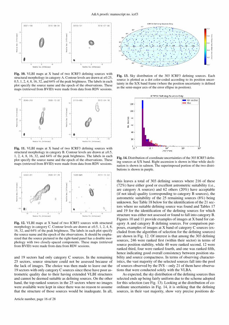
A&A proofs: manuscript no. icrf3
Fig. 10. VLBI maps at X band of two ICRF3 defining sources withstructural morphology in category A. Contour levels are drawn at ±0.25,0.5, 1, 2, 4, 8, 16, 32, and 64% of the peak brightness. The labels in eachplot specify the source name and the epoch of the observations. Thesemaps (retrieved from BVID) were made from data from RDV sessions.
Fig. 11. VLBI maps at X band of two ICRF3 defining sources withstructural morphology in category B. Contour levels are drawn at ±0.5,1, 2, 4, 8, 16, 32, and 64% of the peak brightness. The labels in eachplot specify the source name and the epoch of the observations. Thesemaps (retrieved from BVID) were made from data from RDV sessions.
Fig. 12. VLBI maps at X band of two ICRF3 sources with structuralmorphology in category C. Contour levels are drawn at ±0.5, 1, 2, 4, 8,16, 32, and 64% of the peak brightness. The labels in each plot specifythe source name and the epoch of the observations. It should be empha-sized that the source pictured in the right-hand panel has a double mor-phology with two closely-spaced components. These maps (retrievedfrom BVID) were made from data from RDV sessions.
and 19 sectors had only category C sources. In the remaining25 sectors, source structure could not be assessed because ofthe lack of images. The choice was then made to leave out the19 sectors with only category C sources since these have poor as-trometric quality due to their having extended VLBI structuresand cannot be deemed suitable as defining sources. On the otherhand, the top-ranked sources in the 25 sectors where no imageswere available were kept in since there was no reason to assumethat the structure of those sources would be inadequate. In all,
Fig. 13. Sky distribution of the 303 ICRF3 defining sources. Eachsource is plotted as a dot color-coded according to its position uncer-tainty in the S/X band frame (where the position uncertainty is definedas the semi-major axis of the error ellipse in position).
Fig. 14. Distribution of coordinate uncertainties of the 303 ICRF3 defin-ing sources at S/X band. Right ascension is shown in blue while decli-nation is shown in salmon. The superimposed portion of the two distri-butions is shown in purple.
this leaves a total of 303 defining sources where 216 of these(72%) have either good or excellent astrometric suitability (i.e.,are category A sources) and 62 others (20%) have acceptable(if not ideal) quality (corresponding to category B sources), theastrometric suitability of the 25 remaining sources (8%) beingunknown. See Table 18 below for the identification of the 21 sec-tors where no suitable defining source was found and Tables 17and 19 for the identification of the defining sources for whichstructure was either not assessed or found to fall into category B.Figures 10 and 11 provide examples of images at X band for cat-egory A and category B defining sources. For comparison pur-poses, examples of images at X band of category C sources (ex-cluded from the algorithm of selection for the defining sources)are shown in Fig. 12. Of interest is that among the 303 definingsources, 246 were ranked first (within their sector) in terms ofsource position stability, while 40 were ranked second, 12 wereranked third, four were ranked fourth, and one was ranked fifth,hence indicating good overall consistency between position sta-bility and source compactness. In terms of observing character-istics, the vast majority of the selected sources fall into the poolof sources observed by the IVS – only 21 of them have observa-tions that were conducted solely with the VLBA.
As expected, the sky distribution of the defining sources thusselected ends up being fairly uniform due to the scheme adoptedfor this selection (see Fig. 13). Looking at the distribution of co-ordinate uncertainties in Fig. 14, it is striking that the definingsources, in their vast majority, show very precise positions de-
Article number, page 16 of 28
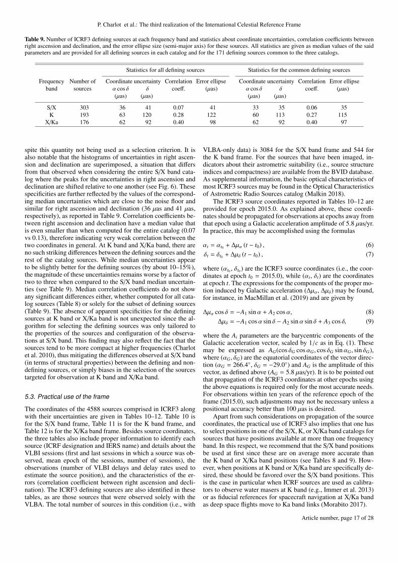
P. Charlot et al.: The third realization of the International Celestial Reference Frame
Table 9. Number of ICRF3 defining sources at each frequency band and statistics about coordinate uncertainties, correlation coefficients betweenright ascension and declination, and the error ellipse size (semi-major axis) for these sources. All statistics are given as median values of the saidparameters and are provided for all defining sources in each catalog and for the 171 defining sources common to the three catalogs.
Statistics for all defining sources Statistics for the common defining sources
Frequency Number of Coordinate uncertainty Correlation Error ellipse Coordinate uncertainty Correlation Error ellipseband sources α cos δ δ coeff. (µas) α cos δ δ coeff. (µas)
(µas) (µas) (µas) (µas)
S/X 303 36 41 0.07 41 33 35 0.06 35K 193 63 120 0.28 122 60 113 0.27 115
X/Ka 176 62 92 0.40 98 62 92 0.40 97
spite this quantity not being used as a selection criterion. It isalso notable that the histograms of uncertainties in right ascen-sion and declination are superimposed, a situation that differsfrom that observed when considering the entire S/X band cata-log where the peaks for the uncertainties in right ascension anddeclination are shifted relative to one another (see Fig. 6). Thesespecificities are further reflected by the values of the correspond-ing median uncertainties which are close to the noise floor andsimilar for right ascension and declination (36 µas and 41 µas,respectively), as reported in Table 9. Correlation coefficients be-tween right ascension and declination have a median value thatis even smaller than when computed for the entire catalog (0.07vs 0.13), therefore indicating very weak correlation between thetwo coordinates in general. At K band and X/Ka band, there areno such striking differences between the defining sources and therest of the catalog sources. While median uncertainties appearto be slightly better for the defining sources (by about 10–15%),the magnitude of these uncertainties remains worse by a factor oftwo to three when compared to the S/X band median uncertain-ties (see Table 9). Median correlation coefficients do not showany significant differences either, whether computed for all cata-log sources (Table 8) or solely for the subset of defining sources(Table 9). The absence of apparent specificities for the definingsources at K band or X/Ka band is not unexpected since the al-gorithm for selecting the defining sources was only tailored tothe properties of the sources and configuration of the observa-tions at S/X band. This finding may also reflect the fact that thesources tend to be more compact at higher frequencies (Charlotet al. 2010), thus mitigating the differences observed at S/X band(in terms of structural properties) between the defining and non-defining sources, or simply biases in the selection of the sourcestargeted for observation at K band and X/Ka band.
5.3. Practical use of the frame
The coordinates of the 4588 sources comprised in ICRF3 alongwith their uncertainties are given in Tables 10–12. Table 10 isfor the S/X band frame, Table 11 is for the K band frame, andTable 12 is for the X/Ka band frame. Besides source coordinates,the three tables also include proper information to identify eachsource (ICRF designation and IERS name) and details about theVLBI sessions (first and last sessions in which a source was ob-served, mean epoch of the sessions, number of sessions), theobservations (number of VLBI delays and delay rates used toestimate the source position), and the characteristics of the er-rors (correlation coefficient between right ascension and decli-nation). The ICRF3 defining sources are also identified in thesetables, as are those sources that were observed solely with theVLBA. The total number of sources in this condition (i.e., with
VLBA-only data) is 3084 for the S/X band frame and 544 forthe K band frame. For the sources that have been imaged, in-dicators about their astrometric suitability (i.e., source structureindices and compactness) are available from the BVID database.As supplemental information, the basic optical characteristics ofmost ICRF3 sources may be found in the Optical Characteristicsof Astrometric Radio Sources catalog (Malkin 2018).
The ICRF3 source coordinates reported in Tables 10–12 areprovided for epoch 2015.0. As explained above, these coordi-nates should be propagated for observations at epochs away fromthat epoch using a Galactic acceleration amplitude of 5.8 µas/yr.In practice, this may be accomplished using the formulas
αt = αt0 + ∆µα (t − t0) , (6)δt = δt0 + ∆µδ (t − t0) , (7)
where (αt0 , δt0 ) are the ICRF3 source coordinates (i.e., the coor-dinates at epoch t0 = 2015.0), while (αt, δt) are the coordinatesat epoch t. The expressions for the components of the proper mo-tion induced by Galactic acceleration (∆µα, ∆µδ) may be found,for instance, in MacMillan et al. (2019) and are given by
∆µα cos δ = −A1 sinα + A2 cosα, (8)∆µδ = −A1 cosα sin δ − A2 sinα sin δ + A3 cos δ, (9)
where the Ai parameters are the barycentric components of theGalactic acceleration vector, scaled by 1/c as in Eq. (1). Thesemay be expressed as AG(cos δG cosαG, cos δG sinαG, sin δG),where (αG, δG) are the equatorial coordinates of the vector direc-tion (αG = 266.4◦, δG = −29.0◦) and AG is the amplitude of thisvector, as defined above (AG = 5.8 µas/yr). It is to be pointed outthat propagation of the ICRF3 coordinates at other epochs usingthe above equations is required only for the most accurate needs.For observations within ten years of the reference epoch of theframe (2015.0), such adjustments may not be necessary unless apositional accuracy better than 100 µas is desired.
Apart from such considerations on propagation of the sourcecoordinates, the practical use of ICRF3 also implies that one hasto select positions in one of the S/X, K, or X/Ka band catalogs forsources that have positions available at more than one frequencyband. In this respect, we recommend that the S/X band positionsbe used at first since these are on average more accurate thanthe K band or X/Ka band positions (see Tables 8 and 9). How-ever, when positions at K band or X/Ka band are specifically de-sired, these should be favored over the S/X band positions. Thisis the case in particular when ICRF sources are used as calibra-tors to observe water masers at K band (e.g., Immer et al. 2013)or as fiducial references for spacecraft navigation at X/Ka bandas deep space flights move to Ka band links (Morabito 2017).
Article number, page 17 of 28
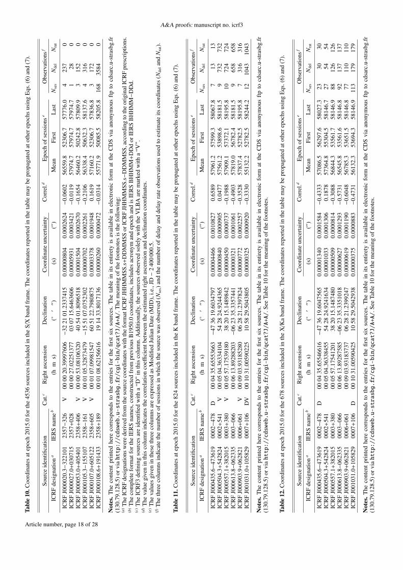
A&A proofs: manuscript no. icrf3Ta
ble
10.C
oord
inat
esat
epoc
h20
15.0
fort
he45
36so
urce
sin
clud
edin
the
S/X
band
fram
e.T
heco
ordi
nate
sre
port
edin
the
tabl
em
aybe
prop
agat
edat
othe
repo
chs
usin
gE
qs.(
6)an
d(7
).
Sour
ceid
entifi
catio
nC
at.c
Rig
htas
cens
ion
Dec
linat
ion
Coo
rdin
ate
unce
rtai
nty
Cor
rel.d
Epo
chof
sess
ions
eO
bser
vatio
nsf
ICR
Fde
sign
atio
na
IER
Sna
me
b(h
ms)
(◦′′′
)(s
)(′′
)M
ean
Firs
tL
ast
Nse
sN
del
Nra
t
ICR
FJ0
0002
0.3−
3221
0123
57−
326
V00
0020
.399
9760
6−
3221
01.2
3374
150.
0000
0804
0.00
0262
4−
0.06
0256
559.
852
306.
757
776.
04
237
0IC
RF
J000
027.
0+03
0715
2357
+02
800
0027
.022
5137
703
0715
.646
3606
0.00
0059
310.
0003
421−
0.01
1957
974.
757
974.
757
974.
71
280
ICR
FJ0
0005
3.0+
4054
0123
58+
406
V00
0053
.081
0632
040
5401
.809
6518
0.00
0015
040.
0002
670−
0.16
5456
460.
250
242.
857
809.
93
152
0IC
RF
J000
105.
3−15
5107
2358−
161
V00
0105
.328
7347
9−
1551
07.0
7523
020.
0000
0702
0.00
0226
1−
0.21
0656
338.
450
632.
358
137.
64
316
0IC
RF
J000
107.
0+60
5122
2358
+60
5V
0001
07.0
9981
547
6051
22.7
9808
750.
0000
3378
0.00
0194
80.
1619
5716
0.2
5230
6.7
5783
6.8
317
20
ICR
FJ0
0010
8.6+
1914
3323
58+
189
0001
08.6
2156
616
1914
33.8
0171
360.
0000
0260
0.00
0047
2−
0.03
1455
771.
950
085.
558
205.
816
835
840
Not
es.T
heco
nten
tpr
inte
dhe
reco
rres
pond
sto
the
entr
ies
for
the
first
six
sour
ces.
The
tabl
ein
itsen
tiret
yis
avai
labl
ein
elec
tron
icfo
rmat
the
CD
Svi
aan
onym
ous
ftp
tocd
sarc
.u-s
tras
bg.fr
(130
.79.
128.
5)or
viahttp://cdsweb.u-strasbg.fr/cgi-bin/qcat?J/A+A/
.The
mea
ning
ofth
efo
otno
tes
isth
efo
llow
ing:
(a)T
heIC
RF
desi
gnat
ions
wer
ede
rived
from
the
sour
ceco
ordi
nate
swith
the
form
atIC
RF
JHH
MM
SS.s
+D
DM
MSS
orIC
RF
JHH
MM
SS.s−
DD
MM
SS,a
ccor
ding
toth
eor
igin
alIC
RF
pres
crip
tions
.(b
)T
heco
mpl
ete
form
atfo
rthe
IER
Sna
mes
,con
stru
cted
from
prev
ious
B19
50.0
coor
dina
tes,
incl
udes
acro
nym
and
epoc
han
dis
IER
SB
HH
MM
+D
Dd
orIE
RS
BH
HM
M−
DD
d.(c
)T
heIC
RF3
defin
ing
sour
ces
are
iden
tified
with
a“D
”in
this
colu
mn.
Add
ition
ally
,the
sour
ces
obse
rved
sole
lyw
ithth
eV
LB
Aar
em
arke
dw
itha
“V”.
(d)
The
valu
egi
ven
inth
isco
lum
nin
dica
tes
the
corr
elat
ion
coeffi
cien
tbet
wee
nth
ees
timat
edri
ghta
scen
sion
and
decl
inat
ion
coor
dina
tes.
(e)
The
valu
esgi
ven
inth
ese
thre
eco
lum
nsar
eex
pres
sed
asM
odifi
edJu
lian
Dat
e(M
JD),
i.e.,
JD−
240
000
0.5.
(f)
The
thre
eco
lum
nsin
dica
teth
enu
mbe
rofs
essi
ons
inw
hich
the
sour
cew
asob
serv
ed(N
ses)
and
the
num
bero
fdel
ayan
dde
lay
rate
obse
rvat
ions
used
toes
timat
eits
coor
dina
tes
(Nde
lan
dN
rat).
Tabl
e11
.Coo
rdin
ates
atep
och
2015
.0fo
rthe
824
sour
ces
incl
uded
inth
eK
band
fram
e.T
heco
ordi
nate
sre
port
edin
the
tabl
em
aybe
prop
agat
edat
othe
repo
chs
usin
gE
qs.(
6)an
d(7
).
Sour
ceid
entifi
catio
nC
at.c
Rig
htas
cens
ion
Dec
linat
ion
Coo
rdin
ate
unce
rtai
nty
Cor
rel.d
Epo
chof
sess
ions
eO
bser
vatio
nsf
ICR
Fde
sign
atio
na
IER
Sna
me
b(h
ms)
(◦′′′
)(s
)(′′
)M
ean
Firs
tL
ast
Nse
sN
del
Nra
t
ICR
FJ0
0043
5.6−
4736
1900
02−
478
D00
0435
.655
5366
3−
4736
19.6
0347
970.
0000
4466
0.00
1082
70.
6589
5796
1.2
5759
9.3
5806
7.8
713
13IC
RF
J000
504.
3+54
2824
0002
+54
1V
0005
04.3
6334
104
5428
24.9
2443
650.
0000
0840
0.00
0090
50.
0477
5756
1.2
5389
8.6
5818
1.5
973
273
2IC
RF
J000
557.
1+38
2015
0003
+38
0V
0005
57.1
7539
180
3820
15.1
4898
420.
0000
0450
0.00
0073
7−
0.19
8857
909.
157
372.
158
195.
810
724
724
ICR
FJ0
0061
3.8−
0623
3500
03−
066
0006
13.8
9288
203−
0623
35.3
3574
410.
0000
0321
0.00
0106
1−
0.49
0357
819.
056
782.
458
181.
59
658
658
ICR
FJ0
0090
3.9+
0628
2100
06+
061
V00
0903
.931
8528
006
2821
.239
7824
0.00
0007
720.
0002
257−
0.35
2857
837.
452
782.
558
195.
87
316
316
ICR
FJ0
0103
1.0+
1058
2900
07+
106
DV
0010
31.0
0590
225
1058
29.5
0438
050.
0000
0325
0.00
0092
0−
0.33
3055
132.
252
782.
558
244.
212
1043
1043
Not
es.T
heco
nten
tpr
inte
dhe
reco
rres
pond
sto
the
entr
ies
for
the
first
six
sour
ces.
The
tabl
ein
itsen
tiret
yis
avai
labl
ein
elec
tron
icfo
rmat
the
CD
Svi
aan
onym
ous
ftp
tocd
sarc
.u-s
tras
bg.fr
(130
.79.
128.
5)or
viahttp://cdsweb.u-strasbg.fr/cgi-bin/qcat?J/A+A/
.See
Tabl
e10
fort
hem
eani
ngof
the
foot
note
s.
Tabl
e12
.Coo
rdin
ates
atep
och
2015
.0fo
rthe
678
sour
ces
incl
uded
inth
eX
/Ka
band
fram
e.T
heco
ordi
nate
sre
port
edin
the
tabl
em
aybe
prop
agat
edat
othe
repo
chs
usin
gE
qs.(
6)an
d(7
).
Sour
ceid
entifi
catio
nC
at.c
Rig
htas
cens
ion
Dec
linat
ion
Coo
rdin
ate
unce
rtai
nty
Cor
rel.d
Epo
chof
sess
ions
eO
bser
vatio
nsf
ICR
Fde
sign
atio
na
IER
Sna
me
b(h
ms)
(◦′′′
)(s
)(′′
)M
ean
Firs
tL
ast
Nse
sN
del
Nra
t
ICR
FJ0
0043
5.6−
4736
1900
02−
478
D00
0435
.655
4661
6−
4736
19.6
0475
650.
0000
1340
0.00
0158
4−
0.43
3357
086.
556
297.
658
027.
323
3030
ICR
FJ0
0050
4.3+
5428
2400
02+
541
0005
04.3
6338
455
5428
24.9
2416
340.
0000
1033
0.00
0130
60.
1878
5736
4.8
5530
4.5
5814
6.7
2754
54IC
RF
J000
557.
1+38
2015
0003
+38
000
0557
.175
4120
138
2015
.148
7480
0.00
0005
090.
0000
814−
0.30
8856
844.
353
561.
758
146.
988
126
126
ICR
FJ0
0061
3.8−
0623
3500
03−
066
0006
13.8
9287
585−
0623
35.3
3510
180.
0000
0627
0.00
0129
3−
0.57
3156
545.
853
561.
658
146.
892
137
137
ICR
FJ0
0090
3.9+
0628
2100
06+
061
0009
03.9
3183
737
0628
21.2
3992
470.
0000
0619
0.00
0119
0−
0.60
4856
785.
353
651.
558
146.
877
110
110
ICR
FJ0
0103
1.0+
1058
2900
07+
106
D00
1031
.005
9042
510
5829
.504
2938
0.00
0003
750.
0000
883−
0.47
3156
132.
353
694.
358
146.
911
317
917
9
Not
es.T
heco
nten
tpr
inte
dhe
reco
rres
pond
sto
the
entr
ies
for
the
first
six
sour
ces.
The
tabl
ein
itsen
tiret
yis
avai
labl
ein
elec
tron
icfo
rmat
the
CD
Svi
aan
onym
ous
ftp
tocd
sarc
.u-s
tras
bg.fr
(130
.79.
128.
5)or
viahttp://cdsweb.u-strasbg.fr/cgi-bin/qcat?J/A+A/
.See
Tabl
e10
fort
hem
eani
ngof
the
foot
note
s.
Article number, page 18 of 28
P. Charlot et al.: The third realization of the International Celestial Reference Frame
6. Analysis of ICRF3
Aside from internal assessments, comparisons of ICRF3 withindependent realizations of the extragalactic frame are essentialto control its quality, its alignment onto the ICRS, and potentialdeformations of the frame. The two independent frames used forthis purpose are the predecessor of ICRF3, ICRF2 (Fey et al.2015), and the recently released Gaia-CRF2 frame in the opticaldomain (Gaia Collaboration et al. 2018). Also important is theassessment of the consistency of the individual source positionsat the three different ICRF3 frequencies and with optical ones inGaia-CRF2 since the measured positions may depend at somelevel on the observed frequency band due to possible physicaloffsets of the emission in the different bands. All such checks arereported below, including a description of the approach devisedfor these comparisons, prior to the presentation of the results.
6.1. Modeling rotations and deformations between catalogs
The scheme that we used for comparing catalogs follows thatdeveloped by Mignard & Klioner (2012) and is based on vectorspherical harmonics decomposition. In this scheme, the coordi-nate differences between catalogs are modeled by a transforma-tion that takes the global rotation between the catalogs into ac-count as well as the low-degree deformations. Mathematically,the corresponding coordinate transformation includes three rota-tions, three “glide” parameters that characterize the dipolar de-formation of the coordinate field (see Mignard & Klioner 2012),and ten quadrupole terms representing degree-2 deformations.Adopting the notation of Titov & Lambert (2013), the coordi-nate differences between the catalogs may be expressed as
∆α cos δ = R1 cosα sin δ + R2 sinα sin δ − R3 cos δ− D1 sinα + D2 cosα+ M20 sin 2δ
+(ERe
21 sinα + EIm21 cosα
)sin δ
−(MRe
21 cosα − MIm21 sinα
)cos 2δ
− 2(ERe
22 sin 2α + EIm22 cos 2α
)cos δ
−(MRe
22 cos 2α − MIm22 sin 2α
)sin 2δ, (10)
∆δ = − R1 sinα + R2 cosα− D1 cosα sin δ − D2 sinα sin δ + D3 cos δ+ E20 sin 2δ
−(ERe
21 cosα − EIm21 sinα
)cos 2δ
−(MRe
21 sinα + MIm21 cosα
)sin δ
−(ERe
22 cos 2α − EIm22 sin 2α
)sin 2δ
+ 2(MRe
22 sin 2α + MIm22 cos 2α
)cos δ, (11)
where the Ri parameters denote the rotations, the Di parametersdenote the glide terms, and the E2i and M2i parameters denotethe poloidal (or electric-type) and toroidal (or magnetic-type)quadrupole terms (each of which with a real and an imaginarypart). For every pair of catalogs that we have compared (see thefollowing subsections), the 16 parameters of the transformationwere obtained by a least-squares fit to the coordinate differencesfor the common sources. In this fit, the coordinate differenceswere weighted by the inverse of the sum of the squared coor-dinate uncertainties in the two catalogs. In order not to bias thedetermination, the fit was performed after excluding the outliers.
As a criterion, a source was considered as an outlier if the an-gular separation between the measured positions in the two cat-alogs normalized by its formal uncertainty (a quantity hereafterreferred to as normalized separation) is larger than 5. Addition-ally, all sources with an angular separation larger than 5 mas orwith an error ellipse in position with a semi-major axis largerthan 5 mas in either catalog were also discarded.
6.2. Comparison with ICRF2
The coordinate transformation described in the previous sectionwas first applied to comparing the ICRF3 S/X band frame withits predecessor, ICRF2, also constructed at S/X band. Since thepurpose of the analysis is to assess the deformations between thetwo frames and not only to check their alignment, the compari-son was carried out based on all sources common to the two cat-alogs and not just the defining sources. After elimination of theoutliers, there were a total of 2918 such sources. To facilitate theevaluation of the results, the 16 parameters derived from the fit(i.e., three rotations, three glide parameters, and ten quadrupoleterms) are plotted in the form of a bar chart in Fig. 15. As ex-pected, the rotations, which reach 15 µas at most, are small.These cannot be exactly zero because the no-net-rotation con-straints imposed to align ICRF3 onto ICRF2 were applied onlyto the ICRF2 defining sources (see Sect. 3.3). Additionally, themeaning of that alignment in the (new) context of inclusion ofGalactic acceleration in the modeling remains somewhat uncer-tain since ICRF2, unlike ICRF3, did not have a reference epoch.Looking at the other parameters, it is striking that the glide termsstand out, whereas all quadrupole terms but one are not signifi-cant. The D2 and D3 glide terms show values of −63± 4 µas and−90 ± 4 µas, respectively, well above the expected deformationsbetween the two frames. The only significant quadrupole param-eter is the E20 term which shows a value of 43 ± 4 µas. All theother quadrupole terms are found to be no larger than 10 µas.
In order to try to get insights into such systematics, we pro-duced several variants of the ICRF3 S/X band frame by chang-ing the reference epoch of the catalog or alternately by not con-sidering Galactic acceleration in the modeling. Interestingly, theD2 and D3 glide terms for these variants were found to vary byseveral tens of microarcseconds in the comparison to ICRF2, inline with the level of the systematics observed for those terms.Such findings are not unexpected since Galactic accelerationmanifests itself as a dipolar deformation in the source coordi-nates (e.g., Titov & Lambert 2013). Moving further, and not-ing that Mignard et al. (2016) mentioned this phenomenon asa possibility for explaining the observed glide between ICRF2and the Gaia Data Release 1 (Gaia DR1) auxiliary quasar solu-tion, we decided to reproduce an equivalent of ICRF2 by con-sidering only the stretch of data used for ICRF2 (i.e., includingonly the VLBI sessions up to March 2009 in the solution) andto make a variant that adds Galactic acceleration in the model-ing, as implemented for ICRF3. To guarantee the maximum con-sistency, those two analyses were conducted by employing thesame software package as that used for ICRF2, namely CALC-SOLVE (see Fey et al. 2015). Looking at the results, we first ob-served that our “reproduced” ICRF2 shows similar deformationsas the original ICRF2 when compared to ICRF3, hence rulingout the possibility that ICRF2 was in error. Most importantly, theICRF2 variant that incorporates Galactic acceleration modelingwas found to have much reduced glide terms compared to theoriginal or reproduced ICRF2. This is illustrated by the bar chartin Fig. 16 which shows that the D2 term has now vanished whilethe D3 term has been cut by more than half (down to a value of
Article number, page 19 of 28
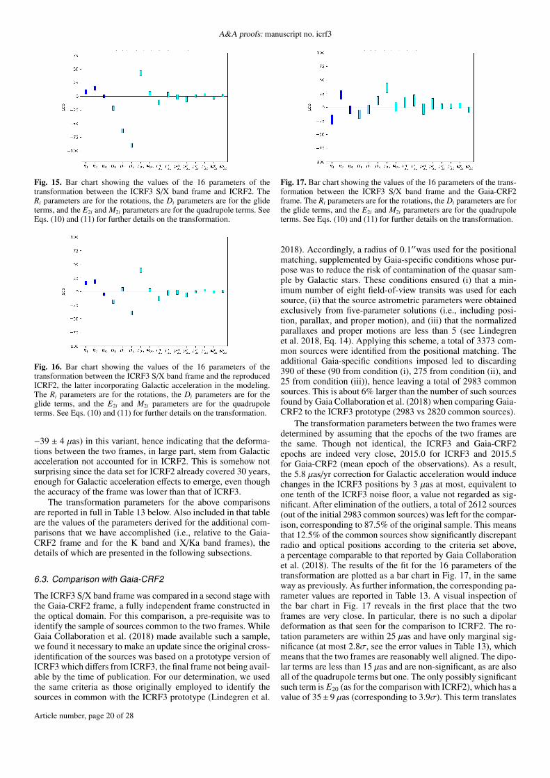
A&A proofs: manuscript no. icrf3
Fig. 15. Bar chart showing the values of the 16 parameters of thetransformation between the ICRF3 S/X band frame and ICRF2. TheRi parameters are for the rotations, the Di parameters are for the glideterms, and the E2i and M2i parameters are for the quadrupole terms. SeeEqs. (10) and (11) for further details on the transformation.
Fig. 16. Bar chart showing the values of the 16 parameters of thetransformation between the ICRF3 S/X band frame and the reproducedICRF2, the latter incorporating Galactic acceleration in the modeling.The Ri parameters are for the rotations, the Di parameters are for theglide terms, and the E2i and M2i parameters are for the quadrupoleterms. See Eqs. (10) and (11) for further details on the transformation.
−39 ± 4 µas) in this variant, hence indicating that the deforma-tions between the two frames, in large part, stem from Galacticacceleration not accounted for in ICRF2. This is somehow notsurprising since the data set for ICRF2 already covered 30 years,enough for Galactic acceleration effects to emerge, even thoughthe accuracy of the frame was lower than that of ICRF3.
The transformation parameters for the above comparisonsare reported in full in Table 13 below. Also included in that tableare the values of the parameters derived for the additional com-parisons that we have accomplished (i.e., relative to the Gaia-CRF2 frame and for the K band and X/Ka band frames), thedetails of which are presented in the following subsections.
6.3. Comparison with Gaia-CRF2
The ICRF3 S/X band frame was compared in a second stage withthe Gaia-CRF2 frame, a fully independent frame constructed inthe optical domain. For this comparison, a pre-requisite was toidentify the sample of sources common to the two frames. WhileGaia Collaboration et al. (2018) made available such a sample,we found it necessary to make an update since the original cross-identification of the sources was based on a prototype version ofICRF3 which differs from ICRF3, the final frame not being avail-able by the time of publication. For our determination, we usedthe same criteria as those originally employed to identify thesources in common with the ICRF3 prototype (Lindegren et al.
Fig. 17. Bar chart showing the values of the 16 parameters of the trans-formation between the ICRF3 S/X band frame and the Gaia-CRF2frame. The Ri parameters are for the rotations, the Di parameters are forthe glide terms, and the E2i and M2i parameters are for the quadrupoleterms. See Eqs. (10) and (11) for further details on the transformation.
2018). Accordingly, a radius of 0.1′′was used for the positionalmatching, supplemented by Gaia-specific conditions whose pur-pose was to reduce the risk of contamination of the quasar sam-ple by Galactic stars. These conditions ensured (i) that a min-imum number of eight field-of-view transits was used for eachsource, (ii) that the source astrometric parameters were obtainedexclusively from five-parameter solutions (i.e., including posi-tion, parallax, and proper motion), and (iii) that the normalizedparallaxes and proper motions are less than 5 (see Lindegrenet al. 2018, Eq. 14). Applying this scheme, a total of 3373 com-mon sources were identified from the positional matching. Theadditional Gaia-specific conditions imposed led to discarding390 of these (90 from condition (i), 275 from condition (ii), and25 from condition (iii)), hence leaving a total of 2983 commonsources. This is about 6% larger than the number of such sourcesfound by Gaia Collaboration et al. (2018) when comparing Gaia-CRF2 to the ICRF3 prototype (2983 vs 2820 common sources).
The transformation parameters between the two frames weredetermined by assuming that the epochs of the two frames arethe same. Though not identical, the ICRF3 and Gaia-CRF2epochs are indeed very close, 2015.0 for ICRF3 and 2015.5for Gaia-CRF2 (mean epoch of the observations). As a result,the 5.8 µas/yr correction for Galactic acceleration would inducechanges in the ICRF3 positions by 3 µas at most, equivalent toone tenth of the ICRF3 noise floor, a value not regarded as sig-nificant. After elimination of the outliers, a total of 2612 sources(out of the initial 2983 common sources) was left for the compar-ison, corresponding to 87.5% of the original sample. This meansthat 12.5% of the common sources show significantly discrepantradio and optical positions according to the criteria set above,a percentage comparable to that reported by Gaia Collaborationet al. (2018). The results of the fit for the 16 parameters of thetransformation are plotted as a bar chart in Fig. 17, in the sameway as previously. As further information, the corresponding pa-rameter values are reported in Table 13. A visual inspection ofthe bar chart in Fig. 17 reveals in the first place that the twoframes are very close. In particular, there is no such a dipolardeformation as that seen for the comparison to ICRF2. The ro-tation parameters are within 25 µas and have only marginal sig-nificance (at most 2.8σ, see the error values in Table 13), whichmeans that the two frames are reasonably well aligned. The dipo-lar terms are less than 15 µas and are non-significant, as are alsoall of the quadrupole terms but one. The only possibly significantsuch term is E20 (as for the comparison with ICRF2), which has avalue of 35± 9 µas (corresponding to 3.9σ). This term translates
Article number, page 20 of 28
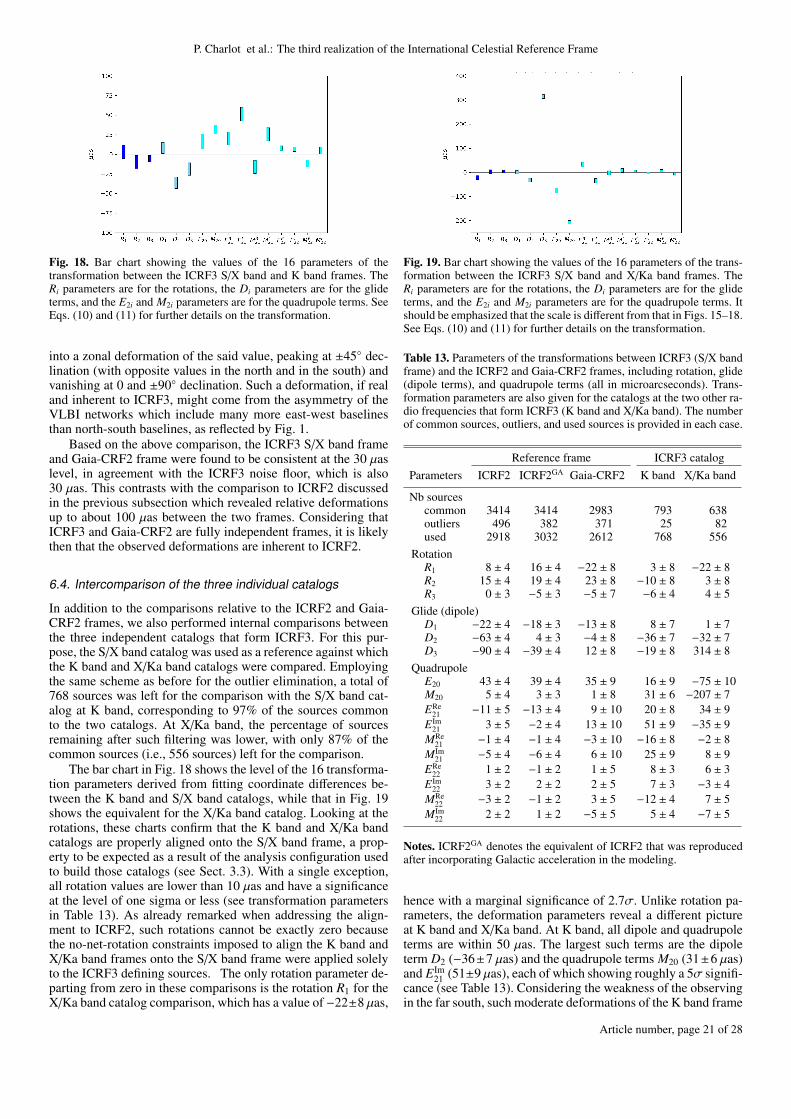
P. Charlot et al.: The third realization of the International Celestial Reference Frame
Fig. 18. Bar chart showing the values of the 16 parameters of thetransformation between the ICRF3 S/X band and K band frames. TheRi parameters are for the rotations, the Di parameters are for the glideterms, and the E2i and M2i parameters are for the quadrupole terms. SeeEqs. (10) and (11) for further details on the transformation.
into a zonal deformation of the said value, peaking at ±45◦ dec-lination (with opposite values in the north and in the south) andvanishing at 0 and ±90◦ declination. Such a deformation, if realand inherent to ICRF3, might come from the asymmetry of theVLBI networks which include many more east-west baselinesthan north-south baselines, as reflected by Fig. 1.
Based on the above comparison, the ICRF3 S/X band frameand Gaia-CRF2 frame were found to be consistent at the 30 µaslevel, in agreement with the ICRF3 noise floor, which is also30 µas. This contrasts with the comparison to ICRF2 discussedin the previous subsection which revealed relative deformationsup to about 100 µas between the two frames. Considering thatICRF3 and Gaia-CRF2 are fully independent frames, it is likelythen that the observed deformations are inherent to ICRF2.
6.4. Intercomparison of the three individual catalogs
In addition to the comparisons relative to the ICRF2 and Gaia-CRF2 frames, we also performed internal comparisons betweenthe three independent catalogs that form ICRF3. For this pur-pose, the S/X band catalog was used as a reference against whichthe K band and X/Ka band catalogs were compared. Employingthe same scheme as before for the outlier elimination, a total of768 sources was left for the comparison with the S/X band cat-alog at K band, corresponding to 97% of the sources commonto the two catalogs. At X/Ka band, the percentage of sourcesremaining after such filtering was lower, with only 87% of thecommon sources (i.e., 556 sources) left for the comparison.
The bar chart in Fig. 18 shows the level of the 16 transforma-tion parameters derived from fitting coordinate differences be-tween the K band and S/X band catalogs, while that in Fig. 19shows the equivalent for the X/Ka band catalog. Looking at therotations, these charts confirm that the K band and X/Ka bandcatalogs are properly aligned onto the S/X band frame, a prop-erty to be expected as a result of the analysis configuration usedto build those catalogs (see Sect. 3.3). With a single exception,all rotation values are lower than 10 µas and have a significanceat the level of one sigma or less (see transformation parametersin Table 13). As already remarked when addressing the align-ment to ICRF2, such rotations cannot be exactly zero becausethe no-net-rotation constraints imposed to align the K band andX/Ka band frames onto the S/X band frame were applied solelyto the ICRF3 defining sources. The only rotation parameter de-parting from zero in these comparisons is the rotation R1 for theX/Ka band catalog comparison, which has a value of −22±8 µas,
Fig. 19. Bar chart showing the values of the 16 parameters of the trans-formation between the ICRF3 S/X band and X/Ka band frames. TheRi parameters are for the rotations, the Di parameters are for the glideterms, and the E2i and M2i parameters are for the quadrupole terms. Itshould be emphasized that the scale is different from that in Figs. 15–18.See Eqs. (10) and (11) for further details on the transformation.
Table 13. Parameters of the transformations between ICRF3 (S/X bandframe) and the ICRF2 and Gaia-CRF2 frames, including rotation, glide(dipole terms), and quadrupole terms (all in microarcseconds). Trans-formation parameters are also given for the catalogs at the two other ra-dio frequencies that form ICRF3 (K band and X/Ka band). The numberof common sources, outliers, and used sources is provided in each case.
Reference frame ICRF3 catalogParameters ICRF2 ICRF2GA Gaia-CRF2 K band X/Ka band
Nb sourcescommon 3414 3414 2983 793 638outliers 496 382 371 25 82used 2918 3032 2612 768 556
RotationR1 8 ± 4 16 ± 4 −22 ± 8 3 ± 8 −22 ± 8R2 15 ± 4 19 ± 4 23 ± 8 −10 ± 8 3 ± 8R3 0 ± 3 −5 ± 3 −5 ± 7 −6 ± 4 4 ± 5
Glide (dipole)D1 −22 ± 4 −18 ± 3 −13 ± 8 8 ± 7 1 ± 7D2 −63 ± 4 4 ± 3 −4 ± 8 −36 ± 7 −32 ± 7D3 −90 ± 4 −39 ± 4 12 ± 8 −19 ± 8 314 ± 8
QuadrupoleE20 43 ± 4 39 ± 4 35 ± 9 16 ± 9 −75 ± 10M20 5 ± 4 3 ± 3 1 ± 8 31 ± 6 −207 ± 7ERe
21 −11 ± 5 −13 ± 4 9 ± 10 20 ± 8 34 ± 9EIm
21 3 ± 5 −2 ± 4 13 ± 10 51 ± 9 −35 ± 9MRe
21 −1 ± 4 −1 ± 4 −3 ± 10 −16 ± 8 −2 ± 8MIm
21 −5 ± 4 −6 ± 4 6 ± 10 25 ± 9 8 ± 9ERe
22 1 ± 2 −1 ± 2 1 ± 5 8 ± 3 6 ± 3EIm
22 3 ± 2 2 ± 2 2 ± 5 7 ± 3 −3 ± 4MRe
22 −3 ± 2 −1 ± 2 3 ± 5 −12 ± 4 7 ± 5MIm
22 2 ± 2 1 ± 2 −5 ± 5 5 ± 4 −7 ± 5
Notes. ICRF2GA denotes the equivalent of ICRF2 that was reproducedafter incorporating Galactic acceleration in the modeling.
hence with a marginal significance of 2.7σ. Unlike rotation pa-rameters, the deformation parameters reveal a different pictureat K band and X/Ka band. At K band, all dipole and quadrupoleterms are within 50 µas. The largest such terms are the dipoleterm D2 (−36±7 µas) and the quadrupole terms M20 (31±6 µas)and EIm
21 (51±9 µas), each of which showing roughly a 5σ signifi-cance (see Table 13). Considering the weakness of the observingin the far south, such moderate deformations of the K band frame
Article number, page 21 of 28
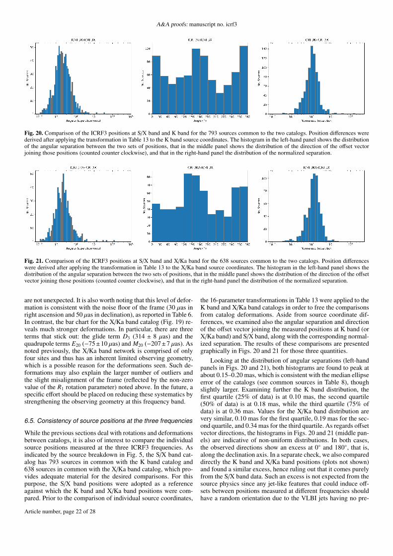
A&A proofs: manuscript no. icrf3
Fig. 20. Comparison of the ICRF3 positions at S/X band and K band for the 793 sources common to the two catalogs. Position differences werederived after applying the transformation in Table 13 to the K band source coordinates. The histogram in the left-hand panel shows the distributionof the angular separation between the two sets of positions, that in the middle panel shows the distribution of the direction of the offset vectorjoining those positions (counted counter clockwise), and that in the right-hand panel the distribution of the normalized separation.
Fig. 21. Comparison of the ICRF3 positions at S/X band and X/Ka band for the 638 sources common to the two catalogs. Position differenceswere derived after applying the transformation in Table 13 to the X/Ka band source coordinates. The histogram in the left-hand panel shows thedistribution of the angular separation between the two sets of positions, that in the middle panel shows the distribution of the direction of the offsetvector joining those positions (counted counter clockwise), and that in the right-hand panel the distribution of the normalized separation.
are not unexpected. It is also worth noting that this level of defor-mation is consistent with the noise floor of the frame (30 µas inright ascension and 50 µas in declination), as reported in Table 6.In contrast, the bar chart for the X/Ka band catalog (Fig. 19) re-veals much stronger deformations. In particular, there are threeterms that stick out: the glide term D3 (314 ± 8 µas) and thequadrupole terms E20 (−75±10 µas) and M20 (−207±7 µas). Asnoted previously, the X/Ka band network is comprised of onlyfour sites and thus has an inherent limited observing geometry,which is a possible reason for the deformations seen. Such de-formations may also explain the larger number of outliers andthe slight misalignment of the frame (reflected by the non-zerovalue of the R1 rotation parameter) noted above. In the future, aspecific effort should be placed on reducing these systematics bystrengthening the observing geometry at this frequency band.
6.5. Consistency of source positions at the three frequencies
While the previous sections deal with rotations and deformationsbetween catalogs, it is also of interest to compare the individualsource positions measured at the three ICRF3 frequencies. Asindicated by the source breakdown in Fig. 5, the S/X band cat-alog has 793 sources in common with the K band catalog and638 sources in common with the X/Ka band catalog, which pro-vides adequate material for the desired comparisons. For thispurpose, the S/X band positions were adopted as a referenceagainst which the K band and X/Ka band positions were com-pared. Prior to the comparison of individual source coordinates,
the 16-parameter transformations in Table 13 were applied to theK band and X/Ka band catalogs in order to free the comparisonsfrom catalog deformations. Aside from source coordinate dif-ferences, we examined also the angular separation and directionof the offset vector joining the measured positions at K band (orX/Ka band) and S/X band, along with the corresponding normal-ized separation. The results of these comparisons are presentedgraphically in Figs. 20 and 21 for those three quantities.
Looking at the distribution of angular separations (left-handpanels in Figs. 20 and 21), both histograms are found to peak atabout 0.15–0.20 mas, which is consistent with the median ellipseerror of the catalogs (see common sources in Table 8), thoughslightly larger. Examining further the K band distribution, thefirst quartile (25% of data) is at 0.10 mas, the second quartile(50% of data) is at 0.18 mas, while the third quartile (75% ofdata) is at 0.36 mas. Values for the X/Ka band distribution arevery similar, 0.10 mas for the first quartile, 0.19 mas for the sec-ond quartile, and 0.34 mas for the third quartile. As regards offsetvector directions, the histograms in Figs. 20 and 21 (middle pan-els) are indicative of non-uniform distributions. In both cases,the observed directions show an excess at 0◦ and 180◦, that is,along the declination axis. In a separate check, we also compareddirectly the K band and X/Ka band positions (plots not shown)and found a similar excess, hence ruling out that it comes purelyfrom the S/X band data. Such an excess is not expected from thesource physics since any jet-like features that could induce off-sets between positions measured at different frequencies shouldhave a random orientation due to the VLBI jets having no pre-
Article number, page 22 of 28
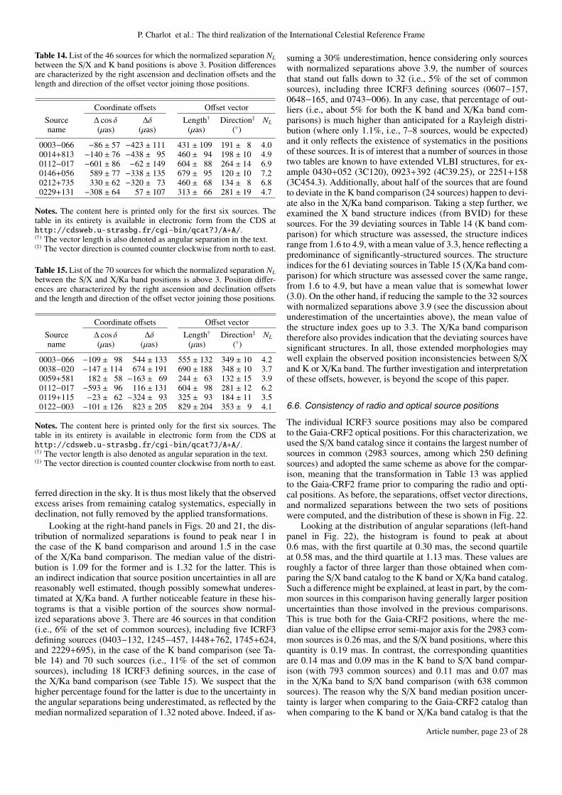
P. Charlot et al.: The third realization of the International Celestial Reference Frame
Table 14. List of the 46 sources for which the normalized separation NLbetween the S/X and K band positions is above 3. Position differencesare characterized by the right ascension and declination offsets and thelength and direction of the offset vector joining those positions.
Coordinate offsets Offset vectorSource ∆ cos δ ∆δ Length† Direction‡ NLname (µas) (µas) (µas) (◦)
0003−066 −86 ± 57 −423 ± 111 431 ± 109 191 ± 8 4.00014+813 −140 ± 76 −438 ± 95 460 ± 94 198 ± 10 4.90112−017 −601 ± 86 −62 ± 149 604 ± 88 264 ± 14 6.90146+056 589 ± 77 −338 ± 135 679 ± 95 120 ± 10 7.20212+735 330 ± 62 −320 ± 73 460 ± 68 134 ± 8 6.80229+131 −308 ± 64 57 ± 107 313 ± 66 281 ± 19 4.7
Notes. The content here is printed only for the first six sources. Thetable in its entirety is available in electronic form from the CDS athttp://cdsweb.u-strasbg.fr/cgi-bin/qcat?J/A+A/.(†) The vector length is also denoted as angular separation in the text.(‡) The vector direction is counted counter clockwise from north to east.
Table 15. List of the 70 sources for which the normalized separation NLbetween the S/X and X/Ka band positions is above 3. Position differ-ences are characterized by the right ascension and declination offsetsand the length and direction of the offset vector joining those positions.
Coordinate offsets Offset vectorSource ∆ cos δ ∆δ Length† Direction‡ NLname (µas) (µas) (µas) (◦)
0003−066 −109 ± 98 544 ± 133 555 ± 132 349 ± 10 4.20038−020 −147 ± 114 674 ± 191 690 ± 188 348 ± 10 3.70059+581 182 ± 58 −163 ± 69 244 ± 63 132 ± 15 3.90112−017 −593 ± 96 116 ± 131 604 ± 98 281 ± 12 6.20119+115 −23 ± 62 −324 ± 93 325 ± 93 184 ± 11 3.50122−003 −101 ± 126 823 ± 205 829 ± 204 353 ± 9 4.1
Notes. The content here is printed only for the first six sources. Thetable in its entirety is available in electronic form from the CDS athttp://cdsweb.u-strasbg.fr/cgi-bin/qcat?J/A+A/.(†) The vector length is also denoted as angular separation in the text.(‡) The vector direction is counted counter clockwise from north to east.
ferred direction in the sky. It is thus most likely that the observedexcess arises from remaining catalog systematics, especially indeclination, not fully removed by the applied transformations.
Looking at the right-hand panels in Figs. 20 and 21, the dis-tribution of normalized separations is found to peak near 1 inthe case of the K band comparison and around 1.5 in the caseof the X/Ka band comparison. The median value of the distri-bution is 1.09 for the former and is 1.32 for the latter. This isan indirect indication that source position uncertainties in all arereasonably well estimated, though possibly somewhat underes-timated at X/Ka band. A further noticeable feature in these his-tograms is that a visible portion of the sources show normal-ized separations above 3. There are 46 sources in that condition(i.e., 6% of the set of common sources), including five ICRF3defining sources (0403−132, 1245−457, 1448+762, 1745+624,and 2229+695), in the case of the K band comparison (see Ta-ble 14) and 70 such sources (i.e., 11% of the set of commonsources), including 18 ICRF3 defining sources, in the case ofthe X/Ka band comparison (see Table 15). We suspect that thehigher percentage found for the latter is due to the uncertainty inthe angular separations being underestimated, as reflected by themedian normalized separation of 1.32 noted above. Indeed, if as-
suming a 30% underestimation, hence considering only sourceswith normalized separations above 3.9, the number of sourcesthat stand out falls down to 32 (i.e., 5% of the set of commonsources), including three ICRF3 defining sources (0607−157,0648−165, and 0743−006). In any case, that percentage of out-liers (i.e., about 5% for both the K band and X/Ka band com-parisons) is much higher than anticipated for a Rayleigh distri-bution (where only 1.1%, i.e., 7–8 sources, would be expected)and it only reflects the existence of systematics in the positionsof these sources. It is of interest that a number of sources in thosetwo tables are known to have extended VLBI structures, for ex-ample 0430+052 (3C120), 0923+392 (4C39.25), or 2251+158(3C454.3). Additionally, about half of the sources that are foundto deviate in the K band comparison (24 sources) happen to devi-ate also in the X/Ka band comparison. Taking a step further, weexamined the X band structure indices (from BVID) for thesesources. For the 39 deviating sources in Table 14 (K band com-parison) for which structure was assessed, the structure indicesrange from 1.6 to 4.9, with a mean value of 3.3, hence reflecting apredominance of significantly-structured sources. The structureindices for the 61 deviating sources in Table 15 (X/Ka band com-parison) for which structure was assessed cover the same range,from 1.6 to 4.9, but have a mean value that is somewhat lower(3.0). On the other hand, if reducing the sample to the 32 sourceswith normalized separations above 3.9 (see the discussion aboutunderestimation of the uncertainties above), the mean value ofthe structure index goes up to 3.3. The X/Ka band comparisontherefore also provides indication that the deviating sources havesignificant structures. In all, those extended morphologies maywell explain the observed position inconsistencies between S/Xand K or X/Ka band. The further investigation and interpretationof these offsets, however, is beyond the scope of this paper.
6.6. Consistency of radio and optical source positions
The individual ICRF3 source positions may also be comparedto the Gaia-CRF2 optical positions. For this characterization, weused the S/X band catalog since it contains the largest number ofsources in common (2983 sources, among which 250 definingsources) and adopted the same scheme as above for the compar-ison, meaning that the transformation in Table 13 was appliedto the Gaia-CRF2 frame prior to comparing the radio and opti-cal positions. As before, the separations, offset vector directions,and normalized separations between the two sets of positionswere computed, and the distribution of these is shown in Fig. 22.
Looking at the distribution of angular separations (left-handpanel in Fig. 22), the histogram is found to peak at about0.6 mas, with the first quartile at 0.30 mas, the second quartileat 0.58 mas, and the third quartile at 1.13 mas. These values areroughly a factor of three larger than those obtained when com-paring the S/X band catalog to the K band or X/Ka band catalog.Such a difference might be explained, at least in part, by the com-mon sources in this comparison having generally larger positionuncertainties than those involved in the previous comparisons.This is true both for the Gaia-CRF2 positions, where the me-dian value of the ellipse error semi-major axis for the 2983 com-mon sources is 0.26 mas, and the S/X band positions, where thisquantity is 0.19 mas. In contrast, the corresponding quantitiesare 0.14 mas and 0.09 mas in the K band to S/X band compar-ison (with 793 common sources) and 0.11 mas and 0.07 masin the X/Ka band to S/X band comparison (with 638 commonsources). The reason why the S/X band median position uncer-tainty is larger when comparing to the Gaia-CRF2 catalog thanwhen comparing to the K band or X/Ka band catalog is that the
Article number, page 23 of 28

A&A proofs: manuscript no. icrf3
Fig. 22. Comparison of the ICRF3 positions at S/X band with the Gaia-CRF2 positions for the 2983 sources common to the two frames. Positiondifferences were derived after applying the transformation in Table 13 to the Gaia-CRF2 source coordinates. The histogram in the left-hand panelshows the distribution of the angular separation between the two sets of positions, that in the middle panel shows the distribution of the direction ofthe offset vector joining those positions (counted counter clockwise), and that in the right-hand panel the distribution of the normalized separation.
Table 16. List of the 653 sources for which the normalized separationNL between the S/X and Gaia-CRF2 positions is above 3. Position dif-ferences are characterized by the right ascension and declination offsetsand the length and direction of the offset vector joining those positions.
Coordinate offsets Offset vectorSource ∆ cos δ ∆δ Length† Direction‡ NLname (µas) (µas) (µas) (◦)
2357−326 −6265 ± 177 −618 ± 289 6295 ± 178 264 ± 3 35.32359−221 −1702 ± 518 1114 ± 567 2034 ± 533 303 ± 16 3.80000−199 −1053 ± 339 1584 ± 359 1902 ± 353 326 ± 10 5.40001−120 1108 ± 319 50 ± 328 1109 ± 319 87 ± 17 3.50003+380 6425 ± 233 −5409 ± 185 8399 ± 214 130 ± 1 39.20003−066 −47 ± 99 227 ± 70 232 ± 71 348 ± 24 3.3
Notes. The content here is printed only for the first six sources. Thetable in its entirety is available in electronic form from the CDS athttp://cdsweb.u-strasbg.fr/cgi-bin/qcat?J/A+A/.(†) The vector length is also denoted as angular separation in the text.(‡) The vector direction is counted counter clockwise from north to east.
common sources fall predominantly into the VLBA-only cate-gory in that comparison, unlike those involved in the K band andX/Ka band comparisons where other sources (i.e., observed alsoby the IVS) predominate. Looking now at the middle panel inFig. 22, which plots the direction of the offset vectors, the dis-tribution is found to be much more uniform than when compar-ing to the K band and X/Ka band catalogs (see Figs. 20 and 21),though there is still a small excess along the declination axis. Thepresence of this excess indicates that the S/X band catalog is notentirely free from declination systematics since there is no rea-son why such systematics should come from the Gaia-CRF2 cat-alog where declination plays no particular role due to the framebeing built from space. The effect, however, is less pronouncedthan that observed in the K band and X/Ka band catalogs.
Of particular interest is the examination of the distribution ofnormalized separations, which is shown in the right-hand panelof Fig. 22. The histogram peaks between 1 and 2, with the me-dian value of the distribution at 1.64, hence indicating possiblyan overall underestimation of the position uncertainties (whichfor the VLBI part would be in contrast with the findings in theprevious subsection) or the presence of real physical offsets be-tween the measured optical and radio positions. Another notice-able feature in that distribution is that a significant portion ofthe sources show large normalized separations (see the higherend of the histogram). Looking at this feature in detail, a total
of 653 sources are found to have a normalized separation largerthan 3, including 59 defining sources. Interestingly, the percent-age of sources that stand out is similar when considering theentire set of common sources or only the defining sources (about22% for the former and 24% for the latter). Furthermore, thereare 144 sources among these that show normalized separationslarger than 10 (corresponding to 4.8% of the common sources),including four defining sources (1.6% of the defining sourcesin common). All 653 sources in this condition (i.e., with a nor-malized separation larger than 3) are listed in Table 16, togetherwith the measured coordinate offsets, offset vectors, and normal-ized separations. The existence of such notable VLBI-Gaia po-sition offsets for a significant portion of the sources was firstrevealed by Mignard et al. (2016), Kovalev et al. (2017), andPetrov & Kovalev (2017b) based on the Gaia DR1 catalog (Lin-degren et al. 2016) and interpreted as the manifestation of opticaljets on scales 1–100 mas (Petrov & Kovalev 2017a). The releaseof the Gaia DR2 catalog (Lindegren et al. 2018) confirmed thosefindings with a higher level of significance (Gaia Collaborationet al. 2018; Petrov et al. 2019; Plavin et al. 2019). Following thelines of the previous section, we examined the structure indicesof the sources with significant positional offsets when available.Out of the 653 sources in Table 16, 267 were found to have anX band structure index in BVID. The mean value of these struc-ture indices is 3.4, with a dichotomy between the 50 definingsources (mean structure index of 2.7) and the 217 other sources(mean structure index of 3.5), hence indicating that sources withsignificant structure predominate. The ICRF3 data thus also sug-gest that the large Gaia-VLBI offsets observed for a notable frac-tion of the sources are likely a manifestation of source structure.
7. Adoption of ICRF3 by the IAU
As stated in the mandate of the working group, ICRF3 waspresented at the 30th IAU General Assembly held in Vienna(Austria) on August 20–31, 2018. The resolution adopted bythe General Assembly, referenced as Resolution B211, resolvedthat the fundamental ICRS realization shall be ICRF3 from Jan-uary 1, 2019, that the organizations responsible for astrometricand geodetic VLBI observing programs (e.g., IVS) shall take ap-propriate measures to both maintain and improve ICRF3, andthat the organizations responsible for defining high-accuracy ref-erence frames at other wavelengths, together with the IERS, shall
11 See Resolution B2 at https://iau.org/static/resolutions/IAU2018_ResolB2_English.pdf.
Article number, page 24 of 28
P. Charlot et al.: The third realization of the International Celestial Reference Frame
take appropriate measures to align those reference frames ontoICRF3 with the highest possible accuracy. As a result of thisadoption, ICRF3 replaced ICRF2 as the fundamental celestialreference frame to use for all applications on January 1, 2019.
8. Evolution of the ICRF
The material presented in the previous sections already providesdirections at which to target prospective VLBI observing alongwith modeling improvements and refinements of the analysisconfiguration in order to enhance the ICRF in the future. Eachof these aspects is discussed in turn in the following paragraphs.
On the observing side, a special effort should be made in thefirst place to strengthen the celestial frame in the far south. Asnoted above, the S/X band frame shows a deficit of sources at themost southern declinations (Fig. 6). While the number of sourcesis similar in the south and in the north for declinations between−35
◦
and +35◦
(1461 vs 1460 sources), the number of sourcesfurther south (< −35
◦
declination) is lower by a factor of 2.5 thanthat further north (> 35
◦
declination) (460 vs 1155 sources). Thesame applies to the K band frame, although the deficit of sourcesin the south is only by a factor of 1.5 in this case. Additionally,it is found that the source position accuracy deteriorates withdeclination (Fig. 9). For such reasons, it is desirable that a properobserving strategy be devised for these two frequency bands toboth increase the source density and augment the source positionaccuracy in the south. Efforts in this direction have already beenengaged and IVS sessions in the south are now strengthened (deWitt et al. 2019). At X/Ka band, the frame is more uniform butsuffers from systematics. The focus of the observing in the futureshould then be placed on reducing these systematics.
A second direction for prospective VLBI observing lies inthe further increase in the source position accuracy for the bulkof the sources in the S/X band frame. Figure 6 shows that thereare two peaks in the distribution of position uncertainties, a pri-mary peak at 100–200 µas capturing the majority of the sourcesand a secondary peak just above the noise floor (30 µas) thatcaptures the roughly 500 sources that have the most precise po-sitions. As noted above, the primary peak (already existing inICRF2) was brought down from 350–700 µas in ICRF2 to thepresent error level thanks to a number of VLBA campaigns con-ducted since 2014 (see Sect. 2.1). Acquiring more data on thecorresponding such 3000 sources will bring this peak furtherdown and even closer to the secondary peak at the noise floor.A factor of 3–4 (the same as that gained from ICRF2 to ICRF3)is still to be gained to merge the two peaks. In this respect, con-tinuation of the VLBA campaigns will be decisive to achieve thisgoal. In this process, observation of the optically bright ICRF3sources (i.e., detected by Gaia) will be also of special interest tostrengthen the alignment between the radio and optical frames.
Above all, it will be essential to monitor closely the definingsources. For this purpose, it would be desirable that these be in-corporated into the regular geodetic VLBI observing programs,such as those carried out by the IVS, in order to control theirastrometric stability. Additionally, it will be important that thesesources be imaged on a regular basis to track potential sourcestructure changes. This especially applies to the 25 ICRF3 defin-ing sources for which we had no VLBI images in hand – thelist of which is given in Table 17 – so that the brightness dis-tribution of those sources, and hence their suitability as defin-ing sources, may be assessed. A specific effort should also bemade toward observing the ICRF3 defining sources at K bandand X/Ka band since not all of them are included the respec-tive catalogs and the amount of data for those that do remains
Table 17. ICRF3 defining sources for which VLBI structure was notassessed prior to their selection as defining sources.
Source names
0009−148 0044−846 0227+403 0642−349 0742−5620802−010 0804−267 0841−607 0926−039 0930−0801016−311 1036−529 1101−536 1245−457 1312−5331325−558 1412−368 1511−558 1556−245 1606−3981753+204 2037+216 2111+400 2121+547 2220−351
Table 18. Identification of the 21 sectors over the celestial sphere whereno suitable defining source was found, either because there is no ICRF3source in that sector or because the source available (indicated in paren-theses) has poor (category C) structure. Each sector is numbered anddefined by a range in right ascension and a range in declination.
Right Asc. DeclinationSector Min Max Min Max Sourcenumber (h m) (h m) (◦) (◦) name
24 01 20 02 40 −26.39 −19.47 (0135−247)26 01 20 02 40 −12.84 −6.38 (0138−097)35 01 20 02 40 51.06 62.73 (0144+584)44 02 40 04 00 −12.84 −6.38 (0238−084)50 02 40 04 00 26.39 33.75 (0333+321)70 04 00 05 20 41.81 51.06 (0420+417)
126 08 00 09 20 62.73 90.00 (0836+710)143 09 20 10 40 51.06 62.73 (0917+624)161 10 40 12 00 51.06 62.73 (1038+528)171 12 00 13 20 −6.38 0.00 (1253−055)178 12 00 13 20 41.81 51.06 (1216+487)230 16 00 17 20 26.39 33.75 (1600+335)239 17 20 18 40 −33.75 −26.39263 18 40 20 00 6.38 12.84 (1947+079)269 18 40 20 00 51.06 62.73 (1954+513)272 20 00 21 20 −62.73 −51.06275 20 00 21 20 −33.75 −26.39 (2000−330)287 20 00 21 20 51.06 62.73 (2037+511)304 21 20 22 40 41.81 51.06 (2200+420)309 22 40 24 00 −51.06 −41.81 (2326−477)318 22 40 24 00 12.84 19.47 (2251+158)
too limited in some cases. Having such a plan is necessary tostrengthen the alignment between the three catalogs in future re-alizations of the ICRF. Beyond that, prospective VLBI observingshould also aim at filling in the 21 empty sectors, which meansto search and identify a suitable defining source for every suchsector. These sectors are identified in Table 18 based on the cor-responding right ascension and declination range. The table alsolists the sources originally selected in these sectors but then dis-carded due to their having too extended (category C) structures(see Sect. 5.2). In the longer term, one should also seek to replacethe 62 defining sources that show moderately extended (i.e. cate-gory B) structures by new ones which are more point-like. Suchsources are listed in Table 19 along with the identification of thecorresponding sectors where new sources are to be found. Forthe goal of finding new sources, either to fill in the empty sectorsin Table 18 or to replace the category B sources in Table 19, theVLBA, again, should be important since it has the capability toobserve weaker sources than geodetic VLBI networks.
Aside from acquiring further VLBI data along the lines de-scribed above, the evolution of the frame will also depend atsome level on the refinements of the modeling. One area whereimprovement is foreseen relates to the determination of the so-
Article number, page 25 of 28
A&A proofs: manuscript no. icrf3
Table 19. Identification of the 62 sectors over the celestial sphere wherethe related ICRF3 defining sources, also specified in the table, showmoderately extended (category B) structures. Each sector is numberedand defined by a range in right ascension and a range in declination.
Right Asc. DeclinationSector Min Max Min Max Defining
number (h m) (h m) (◦) (◦) source
2 00 00 01 20 −62.73 −51.06 0047−57914 00 00 01 20 26.39 33.75 0046+31616 00 00 01 20 41.81 51.06 0110+49519 01 20 02 40 −90.00 −62.73 0230−79031 01 20 02 40 19.47 26.39 0149+21836 01 20 02 40 62.73 90.00 0159+72346 02 40 04 00 0.00 6.38 0305+03953 02 40 04 00 51.06 62.73 0302+62554 02 40 04 00 62.73 90.00 0346+80059 04 00 05 20 −33.75 −26.39 0400−31966 04 00 05 20 12.84 19.47 0507+17972 04 00 05 20 62.73 90.00 0454+84473 05 20 06 40 −90.00 −62.73 0530−72780 05 20 06 40 −12.84 −6.38 0605−08581 05 20 06 40 −6.38 0.00 0539−05790 05 20 06 40 62.73 90.00 0615+82091 06 40 08 00 −90.00 −62.73 0738−67499 06 40 08 00 −6.38 0.00 0743−006
100 06 40 08 00 0.00 6.38 0736+017101 06 40 08 00 6.38 12.84 0748+126105 06 40 08 00 33.75 41.81 0641+392107 06 40 08 00 51.06 62.73 0749+540109 08 00 09 20 −90.00 −62.73 0842−754111 08 00 09 20 −51.06 −41.81 0809−493112 08 00 09 20 −41.81 −33.75 0826−373115 08 00 09 20 −19.47 −12.84 0818−128121 08 00 09 20 19.47 26.39 0834+250125 08 00 09 00 51.06 62.73 0800+618127 09 20 10 40 −90.00 −62.73 1022−665133 09 00 10 40 −19.47 −12.84 1027−186139 09 00 10 40 19.47 26.39 1012+232150 10 40 12 00 −26.39 −19.47 1143−245160 10 40 12 00 41.81 51.06 1150+497173 12 00 13 20 6.38 12.84 1236+077185 13 20 14 40 −33.75 −26.39 1406−267186 13 20 14 40 −26.39 −19.47 1435−218197 13 20 14 40 51.06 62.73 1418+546199 14 40 16 00 −90.00 −62.73 1448−648202 14 40 16 00 −41.81 −33.75 1451−400205 14 40 16 00 −19.47 −12.84 1443−162206 14 40 16 00 −12.84 −6.38 1510−089209 14 40 16 00 6.38 12.84 1502+106213 14 40 16 00 33.75 41.81 1504+377216 14 40 16 00 62.73 90.00 1448+762228 16 00 17 20 12.84 19.47 1717+178233 16 00 17 20 51.06 62.73 1623+578234 16 00 17 20 62.73 90.00 1642+690241 17 20 18 40 −19.47 −12.84 1730−130244 17 20 18 40 0.00 6.38 1725+044253 18 40 20 00 −90.00 −62.73 1935−692254 18 40 20 00 −62.73 −51.06 1925−610256 18 40 20 00 −41.81 −33.75 1954−388257 18 40 20 00 −33.75 −26.39 1921−293260 18 40 20 00 −12.84 −6.38 1937−101276 20 00 21 20 −26.39 −19.47 2037−253284 20 00 21 20 26.39 33.75 2113+293289 21 20 22 40 −90.00 −62.73 2142−758294 21 20 22 40 −26.39 −19.47 2210−257297 21 20 22 40 −6.38 0.00 2216−038306 21 20 22 40 62.73 90.00 2229+695312 22 40 24 00 −26.39 −19.47 2331−240315 22 40 24 00 −6.38 0.00 2335−027
lar system acceleration vector. As the data accumulate, the timespan will also extend, leading to an estimate of the vector ampli-tude with ever increased accuracy. Future data should also revealwhether that vector is directed entirely toward the Galactic cen-ter or is subject to some offset. Additionally, the Gaia mission isexpected to deliver estimates of those parameters in future datareleases, which will further contribute to improving such deter-mination. Another question to be tackled relates to the sourcestructure, which manifests itself through systematics in the VLBIdelay measurements (Xu et al. 2019) and instabilities in the indi-vidual source positions (Gattano et al. 2018). In the future, thoseeffects will become more prominent as the precision of the mea-surements continues to increase, making it necessary to considerthem in the modeling to further increase the quality of the frame.While the corresponding theoretical framework has been put for-ward long ago (Charlot 1990), the practical implementation hasnot been straightforward due to the requirement to have multi-epoch images available for all the sources. While producing suchseries of images is an enormous task, the advent of several im-age databases (Collioud & Charlot 2019; Hunt et al. 2019) nowoffers interesting prospects for the coming years in this area.
Finally, another route to investigate that might possibly helpto enhance the frame lies in exploring alternate analysis config-urations. While the three catalogs that form ICRF3 have beenderived independently, the corresponding data sets could be pro-cessed together. The observing system is largely similar at thethree frequency bands and such a joint analysis should benefitfrom the strengths of each data set, most likely resulting in im-provements of the overall frame. For example, systematics in theX/Ka band catalog (see Sect. 6.4) might end up reduced afterincorporation of the S/X band and K band data sets in the anal-ysis. There are also reasons to expect an even closer alignmentof the three catalogs with this scheme. It should be emphasized,though, that the source positions should be kept as separate pa-rameters at the three frequencies, as otherwise any actual phys-ical offsets, such as those suspected here for a fraction of thesources (see Sect. 6.5), would affect the resulting source positionestimates. It is worth noting that such a multi-frequency analy-sis has been recently tried, though not through using a uniquesoftware package but instead through a combination of normalequations derived at each frequency band, demonstrating thatthere would be some value in investigating further such a com-bination for future realizations of the ICRF (Karbon & Noth-nagel 2019). Going further, one may even consider incorporat-ing data from other space geodetic techniques in the combina-tion. Those techniques include satellite and lunar laser ranging,global navigation satellite systems, and the “doppler orbitogra-phy and radiopositioning integrated by satellite” system, which,together with VLBI, contribute to the realization of the ITRF.While the impact on the celestial frame may be limited, such amulti-technique combination would have the advantage to de-liver unified terrestrial and celestial frames (Seitz et al. 2014).
9. Conclusion
A new realization of the ICRF, denoted as ICRF3, has been pro-duced based on VLBI data acquired over nearly 40 years in threefrequency bands (S/X, K, and X/Ka band). This new realizationis the first multi-frequency celestial reference frame ever gener-ated. Another new feature incorporated in ICRF3 is the modelingof the galactocentric acceleration of the solar system, which con-siders an acceleration vector pointing toward the Galactic centerwith an amplitude of 5.8 µas/yr. The latter was derived by anadjustment directly to the S/X band data. Source positions are
Article number, page 26 of 28
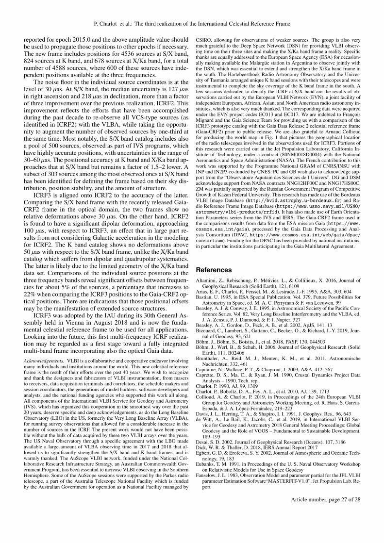
P. Charlot et al.: The third realization of the International Celestial Reference Frame
reported for epoch 2015.0 and the above amplitude value shouldbe used to propagate those positions to other epochs if necessary.The new frame includes positions for 4536 sources at S/X band,824 sources at K band, and 678 sources at X/Ka band, for a totalnumber of 4588 sources, where 600 of these sources have inde-pendent positions available at the three frequencies.
The noise floor in the individual source coordinates is at thelevel of 30 µas. At S/X band, the median uncertainty is 127 µasin right ascension and 218 µas in declination, more than a factorof three improvement over the previous realization, ICRF2. Thisimprovement reflects the efforts that have been accomplishedduring the past decade to re-observe all VCS-type sources (asidentified in ICRF2) with the VLBA, while taking the opportu-nity to augment the number of observed sources by one-third atthe same time. Most notably, the S/X band catalog includes alsoa pool of 500 sources, observed as part of IVS programs, whichhave highly accurate positions, with uncertainties in the range of30–60 µas. The positional accuracy at K band and X/Ka band ap-proaches that at S/X band but remains a factor of 1.5–2 lower. Asubset of 303 sources among the most observed ones at S/X bandhas been identified for defining the frame based on their sky dis-tribution, position stability, and the amount of structure.
ICRF3 is aligned onto ICRF2 to the accuracy of the latter.Comparing the S/X band frame with the recently released Gaia-CRF2 frame in the optical domain, the two frames show norelative deformations above 30 µas. On the other hand, ICRF2is found to have a significant dipolar deformation, approaching100 µas, with respect to ICRF3, an effect that in large part re-sults from not considering Galactic acceleration in the modelingfor ICRF2. The K band catalog shows no deformations above50 µas with respect to the S/X band frame, unlike the X/Ka bandcatalog which suffers from dipolar and quadrupolar systematics.The latter is likely due to the limited geometry of the X/Ka banddata set. Comparisons of the individual source positions at thethree frequency bands reveal significant offsets between frequen-cies for about 5% of the sources, a percentage that increases to22% when comparing the ICRF3 positions to the Gaia-CRF2 op-tical positions. There are indications that those positional offsetsmay be the manifestation of extended source structures.
ICRF3 was adopted by the IAU during its 30th General As-sembly held in Vienna in August 2018 and is now the funda-mental celestial reference frame to be used for all applications.Looking into the future, this first multi-frequency ICRF realiza-tion may be regarded as a first stage toward a fully integratedmulti-band frame incorporating also the optical Gaia data.Acknowledgements. VLBI is a collaborative and cooperative endeavor involvingmany individuals and institutions around the world. This new celestial referenceframe is the result of their efforts over the past 40 years. We wish to recognizeand thank the designers and fabricators of VLBI instrumentation, from masersto receivers, data acquisition terminals and correlators, the schedule makers andsession coordinators, the generations of model builders, software developers andanalysts, and the national funding agencies who supported this work all along.All components of the International VLBI Service for Geodesy and Astrometry(IVS), which has organized this cooperation in the smoothest way over the past20 years, deserve specific and deep acknowledgements, as do the Long BaselineObservatory (LBO) in the US, formerly the Very Long Baseline Array (VLBA),for running survey observations that allowed for a considerable increase in thenumber of sources in the ICRF. The present work would not have been possi-ble without the bulk of data acquired by these two VLBI arrays over the years.The US Naval Observatory through a specific agreement with the LBO madeavailable a large amount of VLBA observing time in 2017 and 2018 that al-lowed us to significantly strengthen the S/X band and K band frames, and iswarmly thanked. The AuScope VLBI network, funded under the National Col-laborative Research Infrastructure Strategy, an Australian Commonwealth Gov-ernment Program, has been essential to increase VLBI observing in the SouthernHemisphere. Some of the AuScope sessions were supported by the Parkes radiotelescope, a part of the Australia Telescope National Facility which is fundedby the Australian Government for operation as a National Facility managed by
CSIRO, allowing for observations of weaker sources. The group is also verymuch grateful to the Deep Space Network (DSN) for providing VLBI observ-ing time on their three sites and making the X/Ka band frame a reality. Specificthanks are equally addressed to the European Space Agency (ESA) for occasion-ally making available the Malargüe station in Argentina to observe jointly withthe DSN, which was essential to extend and strengthen the X/Ka band frame inthe south. The Hartebeesthoek Radio Astronomy Observatory and the Univer-sity of Tasmania arranged unique K band sessions with their telescopes and wereinstrumental to complete the sky coverage of the K band frame in the south. Afew sessions dedicated to densify the ICRF at S/X band are the results of ob-servations carried out by the European VLBI Network (EVN), a joint facility ofindependent European, African, Asian, and North American radio astronomy in-stitutes, which is also very much thanked. The corresponding data were acquiredunder the EVN project codes EC013 and EC017. We are indebted to FrançoisMignard and the Gaia Science Team for providing us with a comparison of theICRF3 prototype catalog with the Gaia Data Release 2 celestial reference frame(Gaia-CRF2) prior to public release. We are also grateful to Arnaud Collioudfor producing the world map in Fig. 1 that pictures the geographical locationof the radio telescopes involved in the observations used for ICRF3. Portions ofthis research were carried out at the Jet Propulsion Laboratory, California In-stitute of Technology, under a contract (80NM0018D0004) with the NationalAeronautics and Space Administration (NASA). The French contribution to thiswork was supported by the Programme National GRAM of CNRS/INSU withINP and IN2P3 co-funded by CNES. PC and GB wish also to acknowledge sup-port from the “Observatoire Aquitain des Sciences de l’Univers”. DG and DSMacknowledge support from NASA contracts NNG12HP00C and NNG17HS00C.ZM was partially supported by the Russian Government Program of CompetitiveGrowth of Kazan Federal University. This research has made use of the BordeauxVLBI Image Database (http://bvid.astrophy.u-bordeaux.fr) and Ra-dio Reference Frame Image Database (https://www.usno.navy.mil/USNO/astrometry/vlbi-products/rrfid). It has also made use of Earth Orienta-tion Parameters series from the IVS and IERS. The Gaia-CRF2 frame used inthe comparisons results from data from the ESA mission Gaia (https://www.cosmos.esa.int/gaia), processed by the Gaia Data Processing and Anal-ysis Consortium (DPAC, https://www.cosmos.esa.int/web/gaia/dpac/consortium). Funding for the DPAC has been provided by national institutions,in particular the institutions participating in the Gaia Multilateral Agreement.
ReferencesAltamimi, Z., Rebischung, P., Métivier, L., & Collilieux, X. 2016, Journal of
Geophysical Research (Solid Earth), 121, 6109Arias, E. F., Charlot, P., Feissel, M., & Lestrade, J.-F. 1995, A&A, 303, 604Bastian, U. 1995, in ESA Special Publication, Vol. 379, Future Possibilities for
Astrometry in Space, ed. M. A. C. Perryman & F. van Leeuwen, 99Beasley, A. J. & Conway, J. E. 1995, in Astronomical Society of the Pacific Con-
ference Series, Vol. 82, Very Long Baseline Interferometry and the VLBA, ed.J. A. Zensus, P. J. Diamond, & P. J. Napier, 327
Beasley, A. J., Gordon, D., Peck, A. B., et al. 2002, ApJS, 141, 13Bizouard, C., Lambert, S., Gattano, C., Becker, O., & Richard, J.-Y. 2019, Jour-
nal of Geodesy, 93, 621Böhm, J., Böhm, S., Boisits, J., et al. 2018, PASP, 130, 044503Böhm, J., Werl, B., & Schuh, H. 2006, Journal of Geophysical Research (Solid
Earth), 111, B02406Brunthaler, A., Reid, M. J., Menten, K. M., et al. 2011, Astronomische
Nachrichten, 332, 461Capitaine, N., Wallace, P. T., & Chapront, J. 2003, A&A, 412, 567Caprette, D. S., Ma, C., & Ryan, J. M. 1990, Crustal Dynamics Project Data
Analysis – 1990, Tech. rep.Charlot, P. 1990, AJ, 99, 1309Charlot, P., Boboltz, D. A., Fey, A. L., et al. 2010, AJ, 139, 1713Collioud, A. & Charlot, P. 2019, in Proceedings of the 24th European VLBI
Group for Geodesy and Astrometry Working Meeting, ed. R. Haas, S. Garcia-Espada, & J. A. López-Fernández, 219–223
Davis, J. L., Herring, T. A., & Shapiro, I. I. 1991, J. Geophys. Res., 96, 643de Witt, A., Le Bail, K., Jacobs, C., et al. 2019, in International VLBI Ser-
vice for Geodesy and Astrometry 2018 General Meeting Proceedings: GlobalGeodesy and the Role of VGOS – Fundamental to Sustainable Development,189–193
Desai, S. D. 2002, Journal of Geophysical Research (Oceans), 107, 3186Dick, W. R. & Thaller, D. 2018, IERS Annual Report 2017Egbert, G. D. & Erofeeva, S. Y. 2002, Journal of Atmospheric and Oceanic Tech-
nology, 19, 183Eubanks, T. M. 1991, in Proceedings of the U. S. Naval Observatory Workshop
on Relativistic Models for Use in Space GeodesyFanselow, J. L. 1983, Observation Model and parameter partial for the JPL VLBI
parameter Estimation Software“MASTERFIT-V1.0”, Jet Propulsion Lab. Re-port
Article number, page 27 of 28
A&A proofs: manuscript no. icrf3
Fey, A. L. & Charlot, P. 1997, ApJS, 111, 95Fey, A. L., Gordon, D., Jacobs, C. S., et al. 2015, AJ, 150, 58Fey, A. L., Ma, C., Arias, E. F., et al. 2004, AJ, 127, 3587Fomalont, E. B., Petrov, L., MacMillan, D. S., Gordon, D., & Ma, C. 2003, AJ,
126, 2562Fricke, W., Schwan, H., Lederle, T., et al. 1988, Veroeffentlichungen des As-
tronomischen Rechen-Instituts Heidelberg, 32, 1Gaia Collaboration, Mignard, F., Klioner, S. A., et al. 2018, A&A, 616, A14Gattano, C., Lambert, S. B., & Le Bail, K. 2018, A&A, 618, A80Gordon, D. 2017, Journal of Geodesy, 91, 735Gordon, D., Jacobs, C., Beasley, A., et al. 2016, AJ, 151, 154Gwinn, C. R., Eubanks, T. M., Pyne, T., Birkinshaw, M., & Matsakis, D. N.
1997, ApJ, 485, 87Herring, T. A. 1986, J. Geophys. Res., 91, 9177Hilton, J. L., Capitaine, N., Chapront, J., et al. 2006, Celestial Mechanics and
Dynamical Astronomy, 94, 351Honma, M., Nagayama, T., Ando, K., et al. 2012, PASJ, 64, 136Hunt, L., Johnson, M., Fey, A., Spitzak, J., & Gordon, D. 2019, in Proceedings of
the 24th European VLBI Group for Geodesy and Astrometry Working Meet-ing, ed. R. Haas, S. Garcia-Espada, & J. A. López-Fernández, 214–218
Immer, K., Reid, M. J., Menten, K. M., Brunthaler, A., & Dame, T. M. 2013,A&A, 553, A117
Jacobs, C. S., Clark, J. E., García-Miró, C., et al. 2012, in 23rd Symposium onSpace Flight Dynamics, 15 pages
Karbon, M. & Nothnagel, A. 2019, A&A, 630, A101Kopeikin, S. M. & Makarov, V. V. 2006, AJ, 131, 1471Kovalev, Y. Y., Petrov, L., Fomalont, E. B., & Gordon, D. 2007, AJ, 133, 1236Kovalev, Y. Y., Petrov, L., & Plavin, A. V. 2017, A&A, 598, L1Kovalevsky, J. 2003, A&A, 404, 743Kovalevsky, J., Lindegren, L., Perryman, M. A. C., et al. 1997, A&A, 323, 620Kurdubov, S. 2007, in Proceedings of the 18th European VLBI for Geodesy and
Astrometry Working Meeting, ed. J. Böhm, A. Pany, & H. Schuh, 79–81Lanyi, G. E., Boboltz, D. A., Charlot, P., et al. 2010, AJ, 139, 1695Le Bail, K., Gipson, J. M., Gordon, D., et al. 2016, AJ, 151, 79Lefèvre, F., Lyard, F. H., Le Provost, C., & Schrama, E. J. O. 2002, Journal of
Atmospheric and Oceanic Technology, 19, 1345Lindegren, L., Hernández, J., Bombrun, A., et al. 2018, A&A, 616, A2Lindegren, L., Lammers, U., Bastian, U., et al. 2016, A&A, 595, A4Ma, C., Arias, E. F., Eubanks, T. M., et al. 1998, AJ, 116, 516MacMillan, D. S., Fey, A., Gipson, J. M., et al. 2019, A&A, 630, A93MacMillan, D. S. & Ma, C. 1994, J. Geophys. Res., 99, 637Malkin, Z. 2016, MNRAS, 461, 1937Malkin, Z. 2018, ApJS, 239, 20Mathews, P. M., Herring, T. A., & Buffett, B. A. 2002, Journal of Geophysical
Research (Solid Earth), 107, 2068Mignard, F. 2002, in EAS Publications Series, Vol. 2, EAS Publications Series,
ed. O. Bienayme & C. Turon, 327–339Mignard, F. & Klioner, S. 2012, A&A, 547, A59Mignard, F., Klioner, S., Lindegren, L., et al. 2016, A&A, 595, A5Morabito, D. D. 2017, Interplanetary Network Progress Report, 211, 1Nilsson, T., Soja, B., Karbon, M., Heinkelmann, R., & Schuh, H. 2015, Earth,
Planets, and Space, 67, 136Noll, C. E. 2010, Advances in Space Research, 45, 1421Nothnagel, A. 2009, Journal of Geodesy, 83, 787Nothnagel, A., Artz, T., Behrend, D., & Malkin, Z. 2017, Journal of Geodesy,
91, 711Petit, G. & Luzum, B. 2010, IERS Technical Note, 36Petrov, L. & Boy, J.-P. 2004, Journal of Geophysical Research (Solid Earth),
109, B03405Petrov, L. & Kovalev, Y. Y. 2017a, MNRAS, 471, 3775Petrov, L. & Kovalev, Y. Y. 2017b, MNRAS, 467, L71Petrov, L., Kovalev, Y. Y., Fomalont, E., & Gordon, D. 2005, AJ, 129, 1163Petrov, L., Kovalev, Y. Y., Fomalont, E. B., & Gordon, D. 2006, AJ, 131, 1872Petrov, L., Kovalev, Y. Y., Fomalont, E. B., & Gordon, D. 2008, AJ, 136, 580Petrov, L., Kovalev, Y. Y., Fomalont, E. B., & Gordon, D. 2011, AJ, 142, 35Petrov, L., Kovalev, Y. Y., & Plavin, A. V. 2019, MNRAS, 482, 3023Plank, L., Lovell, J. E. J., McCallum, J. N., et al. 2017, Journal of Geodesy, 91,
803Plavin, A. V., Kovalev, Y. Y., & Petrov, L. Y. 2019, ApJ, 871, 143Reid, M. J., Menten, K. M., Brunthaler, A., et al. 2014, ApJ, 783, 130Reid, M. J., Menten, K. M., Zheng, X. W., et al. 2009, ApJ, 700, 137Rogers, A. E. E. 1970, Radio Science, 5, 1239Ryan, J. W., Clark, T. A., Ma, C., et al. 1993, in Contributions of Space Geodesy
to Geodynamics: Crustal Dynamics, ed. D. E. Smith & D. L. Turcotte, 37–49Schlüter, W. & Behrend, D. 2007, Journal of Geodesy, 81, 379Schuh, H. & Behrend, D. 2012, Journal of Geodynamics, 61, 68Seitz, M., Steigenberger, P., & Artz, T. 2014, in Earth on the Edge: Science for
a Sustainable Planet, ed. C. Rizos & P. Willis (Berlin, Heidelberg: SpringerBerlin Heidelberg), 215–221
Sovers, O. J., Fanselow, J. L., & Jacobs, C. S. 1998, Reviews of Modern Physics,70, 1393
Sovers, O. J. & Jacobs, C. S. 1996, Observation model and parameter partials forthe JPL VLBI parameter estimation software MODEST, 1996, Tech. rep.
Standish, E. M. 1998, Highlights of Astronomy, 11, 310Titov, O. & Krásná, H. 2018, A&A, 610, A36Titov, O. & Lambert, S. 2013, A&A, 559, A95Titov, O., Lambert, S. B., & Gontier, A.-M. 2011, A&A, 529, A91Titov, O., Tesmer, V., & Boehm, J. 2004, in International VLBI Service for
Geodesy and Astrometry 2004 General Meeting Proceedings, ed. N. R. Van-denberg & K. D. Baver, 267
Vallée, J. P. 2017, Ap&SS, 362, 79Xu, M. H., Anderson, J. M., Heinkelmann, R., et al. 2019, ApJS, 242, 5Xu, M. H., Wang, G. L., & Zhao, M. 2012, A&A, 544, A135
Article number, page 28 of 28
Related Documents