The Theory of the Firm under Perfect Competitionncertbooks.prashanthellina.com/class_12.Economics... · The Theory of the Firm under Perfect Competition ... we study a market environment

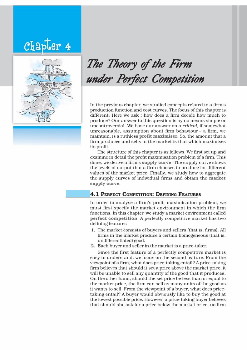
Chapter 4The TheorThe TheorThe TheorThe TheorThe Theory of the Fy of the Fy of the Fy of the Fy of the Firmirmirmirmirmunder Punder Punder Punder Punder Perererererfect Competitionfect Competitionfect Competitionfect Competitionfect Competition

In the previous chapter, we studied concepts related to a firm’sproduction function and cost curves. The focus of this chapter isdifferent. Here we ask : how does a firm decide how much toproduce? Our answer to this question is by no means simple oruncontroversial. We base our answer on a critical, if somewhatunreasonable, assumption about firm behaviour – a firm, wemaintain, is a ruthless profit maximiser. So, the amount that afirm produces and sells in the market is that which maximisesits profit.

The structure of this chapter is as follows. We first set up andexamine in detail the profit maximisation problem of a firm. Thisdone, we derive a firm’s supply curve. The supply curve showsthe levels of output that a firm chooses to produce for differentvalues of the market price. Finally, we study how to aggregatethe supply curves of individual firms and obtain the marketsupply curve.

4.1 PERFECT COMPETITION: DEFINING FEATURES

In order to analyse a firm’s profit maximisation problem, wemust first specify the market environment in which the firmfunctions. In this chapter, we study a market environment calledperfect competition. A perfectly competitive market has twodefining features

1. The market consists of buyers and sellers (that is, firms). Allfirms in the market produce a certain homogeneous (that is,undifferentiated) good.

2. Each buyer and seller in the market is a price-taker.

Since the first feature of a perfectly competitive market iseasy to understand, we focus on the second feature. From theviewpoint of a firm, what does price-taking entail? A price-takingfirm believes that should it set a price above the market price, itwill be unable to sell any quantity of the good that it produces.On the other hand, should the set price be less than or equal tothe market price, the firm can sell as many units of the good asit wants to sell. From the viewpoint of a buyer, what does price-taking entail? A buyer would obviously like to buy the good atthe lowest possible price. However, a price-taking buyer believesthat should she ask for a price below the market price, no firm

will be willing to sell to her. On the other hand, should the price asked begreater than or equal to the market price, the buyer can obtain as manyunits of the good as she desires to buy.

Since this chapter deals exclusively with firms, we probe no further intobuyer behaviour. Instead, we identify conditions under which price-taking isa reasonable assumption for firms. Price-taking is often thought to be areasonable assumption when the market has many firms and buyers haveperfect information about the price prevailing in the market. Why? Let us startwith a situation wherein each firm in the market charges the same (market)price and sells some amount of the good. Suppose, now, that a certain firmraises its price above the market price. Observe that since all firms producethe same good and all buyers are aware of the market price, the firm in questionloses all its buyers. Furthermore, as these buyers switch their purchases toother firms, no “adjustment” problems arise; their demands are readilyaccommodated when there are many firms in the market. Recall, now, that anindividual firm’s inability to sell any amount of the good at a price exceedingthe market price is precisely what the price-taking assumption stipulates.

4.2 REVENUE

We have indicated that in a perfectly competitive market, a firm believes thatit can sell as many units of the good as it wants by setting a price less than orequal to the market price. But, if this is the case, surely there is no reason toset a price lower than the market price. In other words, should the firm desireto sell some amount of the good, the price that it sets is exactly equal to themarket price.

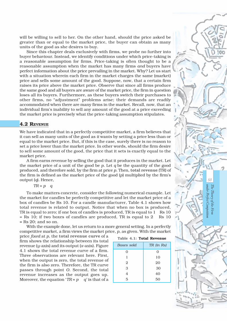
A firm earns revenue by selling the good that it produces in the market. Letthe market price of a unit of the good be p. Let q be the quantity of the goodproduced, and therefore sold, by the firm at price p. Then, total revenue (TR) ofthe firm is defined as the market price of the good (p) multiplied by the firm’soutput (q). Hence,

TR = p × q

To make matters concrete, consider the following numerical example. Letthe market for candles be perfectly competitive and let the market price of abox of candles be Rs 10. For a candle manufacturer, Table 4.1 shows howtotal revenue is related to output. Notice that when no box is produced,TR is equal to zero; if one box of candles is produced, TR is equal to 1 × Rs 10= Rs 10; if two boxes of candles are produced, TR is equal to 2 × Rs 10= Rs 20; and so on.

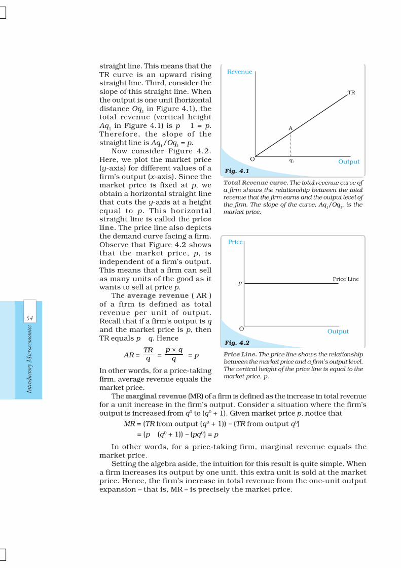
With the example done, let us return to a more general setting. In a perfectlycompetitive market, a firm views the market price, p, as given. With the marketprice fixed at p, the total revenue curve of afirm shows the relationship between its totalrevenue (y-axis) and its output (x-axis). Figure4.1 shows the total revenue curve of a firm.Three observations are relevant here. First,when the output is zero, the total revenue ofthe firm is also zero. Therefore, the TR curvepasses through point O. Second, the totalrevenue increases as the output goes up.Moreover, the equation ‘TR = p × q ’ is that of a

Boxes sold TR (in Rs)

0 0

1 10

2 20

3 30

4 40

5 50

Table 4.1: Total Revenue

53

The T

heory of the Firm

under Perfect C

ompetition

54

Intr

oduc

tory

Mic

roec

onom

ics

straight line. This means that theTR curve is an upward risingstraight line. Third, consider theslope of this straight line. Whenthe output is one unit (horizontaldistance Oq1 in Figure 4.1), thetotal revenue (vertical heightAq1 in Figure 4.1) is p × 1 = p.Therefore, the slope of thestraight line is Aq1/Oq1 = p.

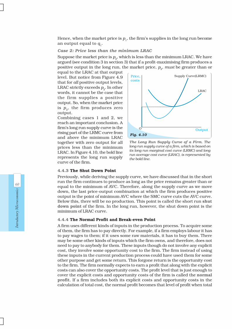
Now consider Figure 4.2.Here, we plot the market price(y-axis) for different values of afirm’s output (x-axis). Since themarket price is fixed at p, weobtain a horizontal straight linethat cuts the y-axis at a heightequal to p. This horizontalstraight line is called the priceline. The price line also depictsthe demand curve facing a firm.Observe that Figure 4.2 showsthat the market price, p, isindependent of a firm’s output.This means that a firm can sellas many units of the good as itwants to sell at price p.

The average revenue ( AR )of a firm is defined as totalrevenue per unit of output.Recall that if a firm’s output is qand the market price is p, thenTR equals p × q. Hence

AR = TRq =

p qq×

= p

In other words, for a price-takingfirm, average revenue equals themarket price.

The marginal revenue (MR) of a firm is defined as the increase in total revenuefor a unit increase in the firm’s output. Consider a situation where the firm’soutput is increased from q0 to (q0 + 1). Given market price p, notice that

MR = (TR from output (q0 + 1)) – (TR from output q0)

= (p × (q0 + 1)) – (pq0) = p

In other words, for a price-taking firm, marginal revenue equals themarket price.

Setting the algebra aside, the intuition for this result is quite simple. Whena firm increases its output by one unit, this extra unit is sold at the marketprice. Hence, the firm’s increase in total revenue from the one-unit outputexpansion – that is, MR – is precisely the market price.

Price Line. The price line shows the relationshipbetween the market price and a firm’s output level.The vertical height of the price line is equal to themarket price, p.

Fig. 4.2

Price

Price Line

O Output

p

Total Revenue curve. The total revenue curve ofa firm shows the relationship between the totalrevenue that the firm earns and the output level ofthe firm. The slope of the curve, Aq

1/Oq

1, is the

market price.

Fig. 4.1

Revenue

TR

O Output

A

q1

55

The T

heory of the Firm

under Perfect C

ompetition

4.3 PROFIT MAXIMISATION

A firm produces and sells a certain amount of a good. The firm’s profit, denotedby π, is defined to be the difference between its total revenue (TR) and its totalcost of production (TC ).1 In other words

π = TR – TCClearly, the gap between TR and TC is the firm’s earnings net of costs.A firm wishes to maximise its profit. The critical question is: at what output

level is the firm’s profit maximised? Assuming that the firm’s output is perfectlydivisible, we now show that if there is a positive output level, q0, at which profitis maximised, then three conditions must hold:

1. The market price, p, is equal to the marginal cost at q0.

2. The marginal cost is non-decreasing at q0.3. In the short run, the market price, p, must be greater than or equal to the

average variable cost at q0. In the long run, the market price, p, must begreater than or equal to the average cost at q

0.

4.3.1 Condition 1

Consider condition 1. We show that condition 1 is true by arguing that a profit-maximising firm will not produce at an output level where market price exceedsmarginal cost or marginal cost exceeds market price. We check both the cases.

Case 1: Price greater than MC is ruled outConsider Figure 4.3 and note that at the output level q2, the market price, p,exceeds the marginal cost. We claim that q

2 cannot be a profit-maximising output

level. Why?Observe that for all output levels slightly to the right of q

2, the market price

continues to exceed the marginal cost. So, pick an output level q3 slightly to the

right of q2 such that the market price exceeds the marginal cost for all output

levels between q2 and q

3.

Suppose, now, that the firm increases its output level from q2 to q

3. The

increase in the total revenue of the firm from this output expansion is justthe market price multiplied by the change in quantity; that is, the area of therectangle q

2q

3CB. On the other hand, the increase in total cost associated

with this output expansion is just the area under the marginal cost curvebetween output levels q

2 and q

3; that is, the area of the region q

2q

3XW. But, a

comparison of the two areas shows that the firm’s profit is higher when itsoutput level is q

3 rather than q

2. But, if this is the case, q

2 cannot be a profit-

maximising output level.

Case 2: Price less than MC is ruled outConsider Figure 4.3 and note that at the output level q

5, the market price, p, is

less than the marginal cost. We claim that q5 cannot be a profit-maximising

output level. Why?Observe that for all output levels slightly to the left of q

5, the market price

remains lower than the marginal cost. So, pick an output level q4 slightly to the

left of q5 such that the market price is less than the marginal cost for all output

levels between q4 and q

5.

Suppose, now, that the firm cuts its output level from q5 to q

4. The decrease

in the total revenue of the firm from this output contraction is just the market

1It is a convention in economics to denote profit with the Greek letter π.

56

Intr

oduc

tory

Mic

roec

onom

ics

price multiplied by the change in quantity; that is, the area of the rectangleq4q5EF. On the other hand, the decrease in total cost brought about by thisoutput contraction is the area under the marginal cost curve between outputlevels q4 and q5; that is, the area of the region q4 q5 ZY. But, a comparison of thetwo areas shows that the firm’s profit is higher when its output level is q

4 rather

than q5. But, if this is the case, q5 cannot be a profit-maximising output level.

4.3.2 Condition 2

Consider the second conditionthat must hold when the profit-maximising output level ispositive. Why is it the case thatthe marginal cost curve cannotslope downwards at the profit-maximising output level? Toanswer this question, refer onceagain to Figure 4.3. Note that atthe output level q

1, the market

price is equal to the marginal cost;however, the marginal cost curveis downward sloping. We claimthat q

1 cannot be a profit-

maximising output level. Why?Observe that for all output

levels slightly to the left of q1,the market price is lower thanthe marginal cost. But, theargument outlined in case 2 of section 3.1 immediately implies that the firm’sprofit at an output level slightly smaller than q

1 exceeds that corresponding to the

output level q1. This being the

case, q1 cannot be a profit-

maximising output level.

4.3.3 Condition 3

Consider the third condition thatmust hold when the profit-maximising output level ispositive. Notice that the thirdcondition has two parts: one partapplies in the short run while theother applies in the long run.

Case 1: Price must be greaterthan or equal to AVC in theshort runWe will show that the statement ofCase 1 (see above) is true byarguing that a profit-maximisingfirm, in the short run, will notproduce at an output level whereinthe market price is lower thanthe AVC.

Conditions 1 and 2 for profit maximisation.The figure is used to demonstrate that when themarket price is p, the output level of a profit-maximising firm cannot be q1 (marginal costcurve, MC, is downward sloping), q2 (marketprice exceeds marginal cost), or q5 (marginal costexceeds market price).

Fig. 4.3

Price,Marginalcost

O Outputq1 q2 q3 q4 q5

p B

W

CY

Z

EFX

MC

Price-AVC Relationship with ProfitMaximisation (Short Run). The figure is usedto demonstrate that a profit-maximising firmproduces zero output in the short run when themarket price, p, is less than the minimum of itsaverage variable cost (AVC). If the firm’s outputlevel is q

1, the firm’s total variable cost exceeds

its revenue by an amount equal to the area ofrectangle pEBA.

Fig. 4.4

Price,costs

O Outputq1

A

E

SMC

B

p

SAC

AVC

57

The T

heory of the Firm

under Perfect C

ompetition

Let us turn to Figure 4.4. Observe that at the output level q1, the market

price p is lower than the AVC. We claim that q1 cannot be a profit-maximisingoutput level. Why?

Notice that the firm’s total revenue at q1 is as follows

TR = Price × Quantity

= Vertical height Op × width Oq1

= The area of rectangle OpAq1

Similarly, the firm’s total variable cost at q1 is as follows

TVC = Average variable cost × Quantity

= Vertical height OE × Width Oq1

= The area of rectangle OEBq1

Now recall that the firm’s profit at q1 is TR – (TVC + TFC); that is, [the area of

rectangle OpAq1] – [the area of rectangle OEBq1] – TFC. What happens if thefirm produces zero output? Since output is zero, TR and TVC are zero as well.Hence, the firm’s profit at zero output is equal to – TFC. But, the area of rectangleOpAq

1 is strictly less than the area of rectangle OEBq

1. Hence, the firm’s profit

at q1 is strictly less than what it obtains by not producing at all. This means, ofcourse, that q

1 cannot be a profit-maximising output level.

Case 2: Price must be greater than or equal to AC in the long runWe will show that the statement of Case 2 (see above) is true by arguing that aprofit-maximising firm, in the long run, will not produce at an output levelwherein the market price is lower than the AC.

Let us turn to Figure 4.5.Observe that at the output levelq

1, the market price p is lower than

the (long run) AC. We claim thatq

1 cannot be a profit-maximising

output level. Why?Notice that the firm’s total

revenue, TR, at q1 is the area of

the rectangle OpAq1 (the product

of price and quantity) while thefirm’s total cost, TC , is the areaof the rectangle OEBq

1 (the

product of average cost andquantity). Since the area ofrectangle OEBq

1 is larger than the

area of rectangle OpAq1, the firm

incurs a loss at the output levelq

1. But, in the long run set-up, a

firm that shuts down productionhas a profit of zero. This means,of course, that q

1 is not a profit-

maximising output level.

4.3.4 The Profit Maximisation Problem: Graphical Representation

Using the material in sections 3.1, 3.2 and 3.3, let us graphically represent afirm’s profit maximisation problem in the short run. Consider Figure 4.6. Notice

Price-AC Relationship with ProfitMaximisation (Long Run). The figure is usedto demonstrate that a profit-maximising firmproduces zero output in the long run when themarket price, p, is less than the minimum of itslong run average cost (LRAC). If the firm’s outputlevel is q1, the firm’s total cost exceeds its revenueby an amount equal to the area of rectangle pEBA.

Fig. 4.5

Price,costs

O Outputq1

A

E

LRMC

B

p

LRAC

58

Intr

oduc

tory

Mic

roec

onom

ics

that the market price is p. Equating the market price with the (short run)marginal cost, we obtain theoutput level q

0. At q

0, observe that

SMC slopes upwards and pexceeds AVC. Since the threeconditions discussed in sections3.1-3.3 are satisfied at q

0, we

maintain that the profit-maximising output level of thefirm is q0.

What happens at q0? The total

revenue of the firm at q0 is thearea of rectangle OpAq

0 (the

product of price and quantity)while the total cost at q

0 is the

area of rectangle OEBq0 (theproduct of short run average costand quantity). So, at q0, the firmearns a profit equal to the area ofthe rectangle EpAB.

4.4 SUPPLY CURVE OF A FIRM

The supply curve of a firm shows the levels of output (plotted on the x-axis)that the firm chooses to produce corresponding to different values of the marketprice (plotted on the y-axis). Of course, for a given market price, the output levelof a profit-maximising firm will depend on whether we are considering the shortrun or the long run. Accordingly, we distinguish between the short run supplycurve and the long run supply curve.

4.4.1 Short Run Supply Curve of a Firm

Let us turn to Figure 4.7 andderive a firm’s short run supplycurve. We shall split thisderivation into two parts. We firstdetermine a firm’s profit-maximising output level when themarket price is greater than orequal to the minimum AVC. Thisdone, we determine the firm’sprofit-maximising output levelwhen the market price is less thanthe minimum AVC.

Case 1: Price is greater thanor equal to the minimum AVCSuppose the market price is p

1,

which exceeds the minimum AVC.We start out by equating p

1 with

SMC on the rising part of the SMCcurve; this leads to the output levelq

1. Note also that the AVC at q

1

Geometric Representation of ProfitMaximisation (Short Run). Given marketprice p, the output level of a profit-maximisingfirm is q0. At q0, the firm’s profit is equal tothe area of rectangle EpAB.

Fig. 4.6

Price,costs

O Outputq1

A

E

SMC

B

pSAC

AVC

Market Price Values. The figure shows theoutput levels chosen by a profit-maximising firmin the short run for two values of the market price:p1 and p2. When the market price is p1, the outputlevel of the firm is q1; when the market price isp2, the firm produces zero output.

Fig. 4.7

Price,costs

O Outputq1

p1

SMC

SAC

AVC

p2

59

The T

heory of the Firm

under Perfect C

ompetition

does not exceed the market price, p1. Thus, all three conditions highlighted in

section 3 are satisfied at q1. Hence, when the market price is p1, the firm’s outputlevel in the short run is equal to q

1.

Case 2: Price is less than the minimum AVCSuppose the market price is p

2, which is less than the minimum AVC. We have

argued (see condition 3 in section 3) that if a profit-maximising firm produces apositive output in the short run, then the market price, p2, must be greater thanor equal to the AVC at that outputlevel. But notice from Figure 4.7that for all positive output levels,AVC strictly exceeds p2. In otherwords, it cannot be the case thatthe firm supplies a positive output.So, if the market price is p

2, the

firm produces zero output.Combining cases 1 and 2, we

reach an important conclusion. Afirm’s short run supply curve isthe rising part of the SMC curvefrom and above the minimum AVCtogether with zero output for allprices strictly less than theminimum AVC. In figure 4.8, thebold line represents the short runsupply curve of the firm.

4.4.2 Long Run Supply Curve of a Firm

Let us turn to Figure 4.9 and derive the firm’s long run supply curve. As in theshort run case, we split the derivation into two parts. We first determine thefirm’s profit-maximising outputlevel when the market price isgreater than or equal to theminimum (long run) AC. Thisdone, we determine the firm’sprofit-maximising output levelwhen the market price is less thanthe minimum (long run) AC.

Case 1: Price greater than orequal to the minimum LRAC

Suppose the market price is p1,

which exceeds the minimumLRAC. Upon equating p

1 with

LRMC on the rising part of theLRMC curve, we obtain outputlevel q1. Note also that the LRACat q

1 does not exceed the market

price, p1. Thus, al l three

condit ions highl ighted insection 3 are satisfied at q

1.

The Short Run Supply Curve of a Firm. Theshort run supply curve of a firm, which is basedon its short run marginal cost curve (SMC) andaverage variable cost curve (AVC), is representedby the bold line.

Fig. 4.8

Price,costs

O Output

SupplyCurve(SMC)

SAC

AVC

Profit maximisation in the Long Run forDifferent Market Price Values. The figureshows the output levels chosen by a profit-maximising firm in the long run for two valuesof the market price: p1 and p2. When the marketprice is p1, the output level of the firm is q1;when the market price is p2, the firm produceszero output.

Fig. 4.9

Price,costs

O Outputq1

p1

LRMC

LRAC

p2

60

Intr

oduc

tory

Mic

roec

onom

ics

Hence, when the market price is p1, the firm’s supplies in the long run become

an output equal to q1.

Case 2: Price less than the minimum LRAC

Suppose the market price is p2, which is less than the minimum LRAC. We have

argued (see condition 3 in section 3) that if a profit-maximising firm produces apositive output in the long run, the market price, p2, must be greater than orequal to the LRAC at that outputlevel. But notice from Figure 4.9that for all positive output levels,LRAC strictly exceeds p

2. In other

words, it cannot be the case thatthe firm supplies a positiveoutput. So, when the market priceis p

2, the firm produces zero

output.Combining cases 1 and 2, wereach an important conclusion. Afirm’s long run supply curve is therising part of the LRMC curve fromand above the minimum LRACtogether with zero output for allprices less than the minimumLRAC. In Figure 4.10, the bold linerepresents the long run supplycurve of the firm.

4.4.3 The Shut Down Point

Previously, while deriving the supply curve, we have discussed that in the shortrun the firm continues to produce as long as the price remains greater than orequal to the minimum of AVC. Therefore, along the supply curve as we movedown, the last price-output combination at which the firm produces positiveoutput is the point of minimum AVC where the SMC curve cuts the AVC curve.Below this, there will be no production. This point is called the short run shutdown point of the firm. In the long run, however, the shut down point is theminimum of LRAC curve.

4.4.4 The Normal Profit and Break-even Point

A firm uses different kinds of inputs in the production process. To acquire someof them, the firm has to pay directly. For example, if a firm employs labour it hasto pay wages to them; if it uses some raw materials, it has to buy them. Theremay be some other kinds of inputs which the firm owns, and therefore, does notneed to pay to anybody for them. These inputs though do not involve any explicitcost, they involve some opportunity cost to the firm. The firm instead of usingthese inputs in the current production process could have used them for someother purpose and get some return. This forgone return is the opportunity costto the firm. The firm normally expects to earn a profit that along with the explicitcosts can also cover the opportunity costs. The profit level that is just enough tocover the explicit costs and opportunity costs of the firm is called the normalprofit. If a firm includes both its explicit costs and opportunity costs in thecalculation of total cost, the normal profit becomes that level of profit when total

The Long Run Supply Curve of a Firm. Thelong run supply curve of a firm, which is based onits long run marginal cost curve (LRMC) and longrun average cost curve (LRAC), is represented bythe bold line.

Fig. 4.10

Price,costs

O Output

Supply Curve(LRMC)

LRAC

61

The T

heory of the Firm

under Perfect C

ompetition

revenue equals total cost, i.e., the zero level of profit. Profit that a firm earns overand above the normal profit is called the super-normal profit. In the long run,a firm does not produce if it earns anything less than the normal profit. In theshort run, however, it may produce even if the profit is less than this level. Thepoint on the supply curve at which a firm earns normal profit is called thebreak-even point of the firm. The point of minimum average cost at which thesupply curve cuts the LRAC curve (in short run, SAC curve) is therefore thebreak-even point of a firm.

Opportunity cost

In economics, one often encounters the concept of opportunity cost.Opportunity cost of some activity is the gain foregone from the second bestactivity. Suppose you have Rs 1,000 which you decide to invest in yourfamily business. What is the opportunity cost of your action? If you do notinvest this money, you can either keep it in the house-safe which will giveyou zero return or you can deposit it in either bank-1 orbank-2 in which case you get an interest at the rate of 10 per cent or 5 percent respectively. So the maximum benefit that you may get from otheralternative activities is the interest from the bank-1. But this opportunitywill no longer be there once you invest the money in your family business.The opportunity cost of investing the money in your family business istherefore the amount of forgone interest from the bank-1.

4.5 DETERMINANTS OF A FIRM’S SUPPLY CURVE

In the previous section, we have seen that a firm’s supply curve is a part of itsmarginal cost curve. Thus, any factor that affects a firm’s marginal cost curve isof course a determinant of its supply curve. In this section, we discuss threesuch factors.

4.5.1 Technological Progress

Suppose a firm uses two factors of production – say, capital and labour – toproduce a certain good. Subsequent to an organisational innovation by the firm,the same levels of capital and labour now produce more units of output. Putdiferently, to produce a given level of output, the organisational innovation allowsthe firm to use fewer units of inputs. It is expected that this will lower the firm’smarginal cost at any level of output; that is, there is a rightward (or downward)shift of the MC curve. As the firm’s supply curve is essentially a segment of theMC curve, technological progress shifts the supply curve of the firm to the right.At any given market price, the firm now supplies more units of output.

4.5.2 Input Prices

A change in input prices also affects a firm’s supply curve. If the price of aninput (say, the wage rate of labour) increases, the cost of production rises. Theconsequent increase in the firm’s average cost at any level of output is usuallyaccompanied by an increase in the firm’s marginal cost at any level of output;that is, there is a leftward (or upward) shift of the MC curve. This means that thefirm’s supply curve shifts to the left: at any given market price, the firm nowsupplies fewer units of output.

62

Intr

oduc

tory

Mic

roec

onom

ics

4.5.3 Unit Tax

A unit tax is a tax that thegovernment imposes per unit saleof output. For example, supposethat the unit tax imposed by thegovernment is Rs 2. Then, if thefirm produces and sells 10 unitsof the good, the total tax that thefirm must pay to the governmentis 10 × Rs 2 = Rs 20.

How does the long run supplycurve of a firm change when a unittax is imposed? Let us turn tofigure 4.11. Before the unit tax isimposed, LRMC0 and LRAC0 are,respectively, the long runmarginal cost curve and the longrun average cost curve of the firm.Now, suppose the governmentputs in place a unit tax of Rs t.Since the firm must pay an extraRs t for each unit of the goodproduced, the firm’s long run average cost and long run marginal cost at anylevel of output increases by Rs t. In Figure 4.11, LRMC1 and LRAC1 are,respectively, the long run marginal cost curve and the long run average costcurve of the firm uponimposition of the unit tax.

Recall that the long runsupply curve of a firm is therising part of the LRMC curvefrom and above the minimumLRAC together with zero outputfor all prices less than theminimum LRAC. Using thisobservation in Figure 4.12, it isimmediate that S0 and S1 are,respectively, the long runsupply curve of the firm beforeand after the imposition of theunit tax. Notice that the unit taxshifts the firm’s long run supplycurve to the left: at any givenmarket price, the firm nowsupplies fewer units of output.

4.6 MARKET SUPPLY CURVE

The market supply curve shows the output levels (plotted on the x-axis) thatfirms in the market produce in aggregate corresponding to different values ofthe market price (plotted on the y-axis).

How is the market supply curve derived? Consider a market with n firms:firm 1, firm 2, firm 3, and so on. Suppose the market price is fixed at p. Then,

Cost Curves and the Unit Tax. LRAC0 andLRMC0 are, respectively, the long run average costcurve and the long run marginal cost curve of afirm before a unit tax is imposed. LRAC1 and LRMC1

are, respectively, the long run average cost curveand the long run marginal cost curve of a firmafter a unit tax of Rs t is imposed.

Fig. 4.11

Costs

O Output

p0

LRMC1

LRAC0

LRMC0

LRAC1

p t0 +

q0

t

Supply Curves and Unit Tax. S0 is the supplycurve of a firm before a unit tax is imposed. Aftera unit tax of Rs t is imposed, S1 represents thesupply curve of the firm.

Fig. 4.12

Price

Output

S1S0

O

p0

p t0 +

q0

63

The T

heory of the Firm

under Perfect C

ompetition

the output produced by the n firms in aggregate is [supply of firm 1 at price p]+ [supply of firm 2 at price p] + ... + [supply of firm n at price p]. In other words,the market supply at price p is the summation of the supplies of individualfirms at that price.

Let us now construct the market supply curve geometrically with just twofirms in the market: firm 1 and firm 2. The two firms have different cost structures.Firm 1 will not produce anything if the market price is less than 1p while firm 2will not produce anything if the market price is less than 2p . Assume also that

2p is greater than 1p .In panel (a) of Figure 4.13 we have the supply curve of firm 1, denoted by

S1; in panel (b), we have the supply curve of firm 2, denoted by S2. Panel (c) ofFigure 4.13 shows the market supply curve, denoted by Sm. When the marketprice is strictly below 1p , both firms choose not to produce any amount of thegood; hence, market supply will also be zero for all such prices. For a marketprice greater than or equal to 1p but strictly less than 2p , only firm 1 will producea positive amount of the good. Therefore, in this range, the market supply curvecoincides with the supply curve of firm 1. For a market price greater than orequal to 2p , both firms will have positive output levels. For example, consider asituation wherein the market price assumes the value p

3 (observe that p

3

exceeds 2p ). Given p3, firm 1 supplies q

3 units of output while firm 2 supplies q

4

units of output. So, the market supply at price p3 is q5, where q5 = q3 + q4. Noticehow the market supply curve, S

m, in panel (c) is being constructed: we obtain S

m

by taking a horizontal summation of the supply curves of the two firms in themarket, S

1 and S

2.

It should be noted that the market supply curve has been derived for a fixednumber of firms in the market. As the number of firms changes, the marketsupply curve shifts as well. Specifically, if the number of firms in the marketincreases (decreases), the market supply curve shifts to the right (left).

We now supplement the graphical analysis given above with a relatednumerical example. Consider a market with two firms: firm 1 and firm 2. Let thesupply curve of firm 1 be as follows

S1(p) = 0 : 10

– 10 : 10

p

p p

<⎧⎨ ≥⎩

The Market Supply Curve Panel. (a) shows the supply curve of firm 1. Panel (b) shows thesupply curve of firm 2. Panel (c) shows the market supply curve, which is obtained by takinga horizontal summation of the supply curves of the two firms.

Fig. 4.13

Price

O Output

p1

O O

S1

q3q4 q5

S2

Sm

p2

p3

(a) (b) (c)

64

Intr

oduc

tory

Mic

roec

onom

ics

Notice that S1(p) indicates that (1) firm 1 produces an output of 0 if the market

price, p, is strictly less than 10, and (2) firm 1 produces an output of (p – 10) ifthe market price, p, is greater than or equal to 10. Let the supply curve of firm 2be as follows

S2(p) =

0 : 15

– 15 : 15

p

p p

<⎧⎨ ≥⎩

The interpretation of S2(p) is identical to that of S1(p), and is, hence, omitted.Now, the market supply curve, S

m(p), simply sums up the supply curves of the

two firms; in other words

Sm(p) = S1(p) + S2(p)

But, this means that Sm(p) is as follows

Sm(p) =

0 : 10

– 10 : 10 15

( – 10) ( – 15) 2 – 25 : 15

p

p p and p

p p p p

<⎧⎪ ≥ <⎨⎪ + = ≥⎩

4.7 PRICE ELASTICITY OF SUPPLY

The price elasticity of supply of a good measures the responsiveness of quantitysupplied to changes in the price of the good. More specifically, the price elasticityof supply, denoted by e

S, is defined as follows

Price elasticity of supply (eS) =

Percentage change in quantity suppliedPercentage change in price

Given the market supply curve of a good (that is, Sm(p)), let q0 be the quantity

of the good supplied to the market when its market price is p0. For some reason,the market price of the good changes from p0 to p1. Let q1 be the quantity ofthe good supplied to the market when the market price is p1. Notice thatwhen the market price moves from p0 to p1, the percentage change in price is

100 ×

1 0

0

( – )p pp

; similarly, when the quantity supplied moves from q0 to q1,

the percentage change in quantity supplied is 100 ×

1 0

0

( – )q qq

. So

eS = ××

1 0 0

1 0 0

100 ( – )/100 ( – )/

q q q

p p p =

1 0

1 0

/ –1/ –1

q qp p

To make matters concrete, consider the following numerical example. Supposethe market for cricket balls is perfectly competitive. When the price of a cricket ballis Rs10, let us assume that 200 cricket balls are produced in aggregate by the firmsin the market. When the price of a cricket ball rises to Rs 30, let us assume that 1,000cricket balls are produced in aggregate by the firms in the market. Then

1. (1

0 1q

q − ) = (1,000/200 – 1) = 4,

2. (1

0 1p

p − ) = (30/10 – 1) = 2,

3. eS =

42 = 2.

65

The T

heory of the Firm

under Perfect C

ompetition

When the supply curve is vertical, supply is completely insensitive to priceand the elasticity of supply is zero. In other cases, when supply curve ispositively sloped, with a rise in price, supply rises and hence, the elasticity ofsupply is positive. Like the price elasticity of demand, the price elasticity ofsupply is also independent of units.

4.7.1 The Geometric Method

Consider the Figure 4.11. Panel (a) shows a straight line supply curve. S is a pointon the supply curve. It cuts the price-axis at its positive range and as we extendthe straight line, it cuts the quantity-axis at M which is at its negative range. Theprice elasticity of this supply curve at the point S is given by the ratio, Mq0/Oq0.For any point S on such a supply curve, we see that Mq

0 > Oq

0. The elasticity at

any point on such a supply curve, therefore, will be greater than 1.In panel (c) we consider a straight line supply curve and S is a point on it. It

cuts the quantity-axis at M which is at its positive range. Again the price elasticityof this supply curve at the point S is given by the ratio, Mq

0/Oq

0. Now, Mq

0 < Oq

0

and hence, eS < 1. S can be any point on the supply curve, and therefore at allpoints on such a supply curve e

S < 1.

Now we come to panel (b). Here the supply curve goes through the origin.One can imagine that the point M has coincided with the origin here, i.e., Mq

0

has become equal to Oq0. The price elasticity of this supply curve at the point Sis given by the ratio, Oq

0/Oq

0 which is equal to 1. At any point on a straight line,

supply curve going through the origin price elasticity will be one.

Price Elasticity Associated with Straight Line Supply Curves. In panel (a), price elasticity(eS ) at S is greater than 1. In panel (b), price elasticity (eS) at S is equal to 1. In panel (c), priceelasticity (eS) at S is less than 1.

• In a perfectly competitive market, firms are price-takers.

• The total revenue of a firm is the market price of the good multiplied by the firm’soutput of the good.

• For a price-taking firm, average revenue is equal to market price.

• For a price-taking firm, marginal revenue is equal to market price.

• The demand curve that a firm faces in a perfectly competitive market is perfectlyelastic; it is a horizontal straight line at the market price.

• The profit of a firm is the difference between total revenue earned and total costincurred.

Su

mm

ary

Su

mm

ary

Su

mm

ary

Su

mm

ary

Su

mm

ary

Fig. 4.14(a) (b) (c)

Price Price Price

Output Output Output

p0 p0 p0

q0 q0q0

S S S

M O OO M

66

Intr

oduc

tory

Mic

roec

onom

ics

• If there is a positive level of output at which a firm’s profit is maximised in theshort run, three conditions must hold at that output level

(i) p = SMC(ii) SMC is non-decreasing(iii) p ≥ AV C.

• If there is a positive level of output at which a firm’s profit is maximised in thelong run, three conditions must hold at that output level

(i) p = LRMC

(ii) LRMC is non-decreasing

(iii) p ≥ LRAC.

• The short run supply curve of a firm is the rising part of the SMC curve from andabove minimum AVC together with 0 output for all prices less than the minimumAVC.

• The long run supply curve of a firm is the rising part of the LRMC curve from andabove minimum LRAC together with 0 output for all prices less than the minimumLRAC.

• Technological progress is expected to shift the supply curve of a firm to the right.

• An increase (decrease) in input prices is expected to shift the supply curve of afirm to the left (right).

• The imposition of a unit tax shifts the supply curve of a firm to the left.

• The market supply curve is obtained by the horizontal summation of the supplycurves of individual firms.

• The price elasticity of supply of a good is the percentage change in quantitysupplied due to one per cent change in the market price of the good.

KKKK Key

Con

cept

sey

Con

cept

sey

Con

cept

sey

Con

cept

sey

Con

cept

s Perfect competition Revenue, Profit

Profit maximisation Firms supply curve

Market supply curve Price elasticity of supply

Ex

erci

ses

Ex

erci

ses

Ex

erci

ses

Ex

erci

ses

Ex

erci

ses 1. What are the characteristics of a perfectly competitive market?

2. How are the total revenue of a firm, market price, and the quantity sold by thefirm related to each other?

3. What is the ‘price line’?

4. Why is the total revenue curve of a price-taking firm an upward-sloping straightline? Why does the curve pass through the origin?

5. What is the relation between market price and average revenue of a price-taking firm?

6. What is the relation between market price and marginal revenue of a price-taking firm?

7. What conditions must hold if a profit-maximising firm produces positive outputin a competitive market?

8. Can there be a positive level of output that a profit-maximising firm producesin a competitive market at which market price is not equal to marginal cost?Give an explanation.

67

The T

heory of the Firm

under Perfect C

ompetition

9. Will a profit-maximising firm in a competitive market ever produce a positivelevel of output in the range where the marginal cost is falling? Give anexplanation.

10. Will a profit-maximising firm in a competitive market produce a positive level ofoutput in the short run if the market price is less than the minimum of AVC?Give an explanation.

11. Will a profit-maximising firm in a competitive market produce a positive level ofoutput in the long run if the market price is less than the minimum of AC?Give an explanation.

12. What is the supply curve of a firm in the short run?

13. What is the supply curve of a firm in the long run?

14. How does technological progress affect the supply curve of a firm?

15. How does the imposition of a unit tax affect the supply curve of a firm?

16. How does an increase in the price of an input affect the supply curve of a firm?

17. How does an increase in the number of firms in a market affect the marketsupply curve?

18. What does the price elasticity of supply mean? How do we measure it?

19. Compute the total revenue, marginalrevenue and average revenue schedulesin the following table. Market price of eachunit of the good is Rs 10.

20. The following table shows thetotal revenue and total costschedules of a competitivefirm. Calculate the profit ateach output level. Determinealso the market price of thegood.

21. The following table shows the total costschedule of a competitive firm. It is given thatthe price of the good is Rs 10. Calculate theprofit at each output level. Find the profitmaximising level of output.

Quantity Sold TR MR AR

0123456

Quantity Sold TR (Rs) TC (Rs) Profit

0 0 51 5 72 10 103 15 124 20 155 25 236 30 337 35 40

Price (Rs) TC (Rs)

0 51 152 223 274 315 386 497 638 819 101

10 123

68

Intr

oduc

tory

Mic

roec

onom

ics

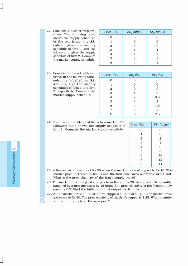
22. Consider a market with twofirms. The following tableshows the supply schedulesof the two firms: the SS1

column gives the supplyschedule of firm 1 and theSS2 column gives the supplyschedule of firm 2. Computethe market supply schedule.

23. Consider a market with twofirms. In the following table,columns labelled as SS1

and SS2 give the supplyschedules of firm 1 and firm2 respectively. Compute themarket supply schedule.

24. There are three identical firms in a market. Thefollowing table shows the supply schedule offirm 1. Compute the market supply schedule.

25. A firm earns a revenue of Rs 50 when the market price of a good is Rs 10. Themarket price increases to Rs 15 and the firm now earns a revenue of Rs 150.What is the price elasticity of the firm’s supply curve?

26. The market price of a good changes from Rs 5 to Rs 20. As a result, the quantitysupplied by a firm increases by 15 units. The price elasticity of the firm’s supplycurve is 0.5. Find the initial and final output levels of the firm.

27. At the market price of Rs 10, a firm supplies 4 units of output. The market priceincreases to Rs 30. The price elasticity of the firm’s supply is 1.25. What quantitywill the firm supply at the new price?

Price (Rs) SS1 (units) SS

2 (units)

0 0 01 0 02 0 03 1 14 2 25 3 36 4 4

Price (Rs) SS1 (kg) SS

2 (kg)

0 0 01 0 02 0 03 1 04 2 0.55 3 16 4 1.57 5 28 6 2.5

Price (Rs) SS1 (units)

0 01 02 23 44 65 86 107 128 14