The Text Feature Analyser

49

The Text Feature Analyser – a Flexible Tool for Comparing

Different Levels of Text Complexity

MARTIN WEISSER

CHEMNITZ UNIVERSITY OF TECHNOLOGY

The following article describes the Text Feature Analyser, an analysis

tool that helps the user to conduct automatic analyses on texts, based on

features that may serve as indicators to the texts’ complexity, genre,

specificity/’scientificness’, etc. These features can easily be changed, or

new ones added, to customise the analysis according to the user’s needs

and expectations towards the text. A sample analysis of two different

texts, dealing with the same subject matter, will be conducted towards the

end of the article in order to demonstrate the relevance of some of the

pre-defined features.

MOTIVATION FOR THE TOOL

The Text Feature Analyser was written in order to try and provide a solution to

a very common problem in dealing with texts written by native and non-native

writers of Academic English, namely the need to establish an objective basis for

the comparison of such texts with regard to their general, objectively observable

and measurable features. Although the goals in writing the tool were not

originally specifically and exclusively geared towards the study of complexity,

ultimately its ‘genesis’ is due to the aim of identifying means of modelling

specific properties that may help us to identify indicators for determining the

degree of complexity in any piece of writing.

PREVIOUS ATTEMPTS AT MEASURING TEXTUAL FEATURES

As already hinted at above, complexity is a phenomenon that is multi-facetted

and so far, no clear indicators of what makes a text complex have been identified,

although there have been different attempts. Ventola (1996) provides an

interesting introduction to some of the ideas underlying the controversy writers

of academic materials may experience when trying to find advice on which

appropriate style(s) to use, as well as to some of the measures that different

researchers have employed in order to try and measure complexity and

readability in texts. Many of the latter, however, seem to have mainly

concentrated on lexical density (LD; Ure, 1971) and are frequently based on

measures that are difficult to extract automatically from text, such as the number

of syllables (Ellis & Hopkins, 1985) or clauses (Halliday, 1985) in a text,

50

paragraph, or sentence, and their relation to the overall number of words in a

document or exclusively restricted to content words.

The measures/indices Ventola describes in her article include the Fog Index

(FOG; Ellis & Hopkins, 1985), as well as two different variants of LD, one as

defined by Ure (1971), the other a modification of the former, defined by

Halliday (1985). Out of the three indices, FOG is the only one which includes a

factor for the number of syllables in the unit of analysis (a passage of

approximately 100 words), and is calculated based on average sentence length (=

number of sentences/word count) plus the number of 3+ syllable words,

multiplied by a factor of 0.4. Its index is based on the raw number of all word

tokens in the unit of analysis. The two LD measures, in contrast, are based on

ratios that are based not on raw token frequencies, but on the frequencies of

lexical items (i.e. content words). Ure’s LD index measures the ratio of content

words to the total number of tokens in the text (expressed as a percentage value),

whereas Halliday’s LD simply gives the ratio of content words to clauses in the

passage/document.

A different and more complex approach to identifying important textual

features is represented by Biber’s multi-dimensional analysis of text categories

(c.f. Biber, 1988 & 2006). Although his approach is not primarily aimed at

identifying features of complexity, some of the features that characterise texts

according to his dimensions and situate them on a continuum from spoken to

written registers are also relevant to the topic of complexity. Biber’s method of

analysis, however, is to a large extent based on tagged corpora, something that

cannot easily be replicated in a relatively small-scale program, such as the Text

Feature Analyser. Despite this fact, the Text Feature Analyser already manages

to incorporate and measure many of the features that form part of Biber’s

categories, as well as the ability to easily add further features, as will be

discussed in a later section.

DESIGN OF THE TOOL

The tool is written in the programming language Perl, a language that is highly

suited to the task of conducting linguistic analyses, not least because its designer,

Larry Wall, is also a linguist. One of the main design features of Perl is that it

enables the programmer to easily specify complex textual patterns that can be

matched against any piece of text and counted or manipulated. The Feature

Analyser relies heavily on this in order to be able to read in a given text

paragraph by paragraph, split up these paragraphs into sentences, and store the

latter in a list that can later be manipulated in order to obtain word frequency

counts, type/token ratios, etc.

The tool itself is split into four modular parts, one document object, one

statistics control object, one statistics calculation module, and the graphical user

interface (GUI) that allows the user to interact conveniently with the other parts

MARTIN WEISSER

51

of the program, make/edit feature selections, or produce descriptive statistics of

the individual features chosen. The results are displayed in a text window, but

can also be exported to a format that can be read into a spreadsheet application

(such as MS Excel) or a database for further statistical analysis. Two additional

text files are used to control the analysis features that are compiled and made

available by the program.

USING THE TOOL

Running the Text Feature Analyser

Although the Text Feature Analyser has a graphical user interface (GUI),

similar to the one most people are used to from Windows programs, it needs to

be run from the command line/shell or via a desktop shortcut on Windows

systems. No installation is necessary, but a Perl interpreter has to be installed on

the system, and the program folder copied to a convenient location, such as the

user’s home folder. The program itself is portable and can be run on MS

Windows, as well as on Linux or other Unix systems.

Once the program has been copied to the computer, it can be started by either

typing ‘perl TextAnalyser.pl’ or simply ‘TextAnalyser.pl’, if the system has been

appropriately configured, on the command line. If a desktop shortcut has been set

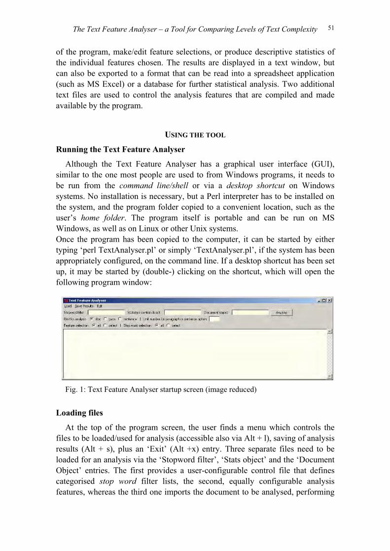
up, it may be started by (double-) clicking on the shortcut, which will open the

following program window:

Fig. 1: Text Feature Analyser startup screen (image reduced)

Loading files

At the top of the program screen, the user finds a menu which controls the

files to be loaded/used for analysis (accessible also via Alt + l), saving of analysis

results (Alt + s), plus an ‘Exit’ (Alt +x) entry. Three separate files need to be

loaded for an analysis via the ‘Stopword filter’, ‘Stats object’ and the ‘Document

Object’ entries. The first provides a user-configurable control file that defines

categorised stop word filter lists, the second, equally configurable analysis

features, whereas the third one imports the document to be analysed, performing

The Text Feature Analyser – a Tool for Comparing Levels of Text Complexity

52

a few separate steps when reading the file into memory. Each action for loading a

file can also be triggered by double-clicking on the appropriate text box. The user

is then provided with a graphical selection dialogue which enables him/her to

navigate to an appropriate folder and select the chosen file. If the user cancels

such a dialogue, an appropriate default file will automatically selected to prevent

the program from producing an error if an analysis without the appropriate

control files is inadvertedly started.

The document to be analysed currently has to be in plain text format, i.e. may

only contain unformatted text, with each paragraph being separated from the next

via two hard returns (line breaks). Further import filters, e.g. for web pages or

Word documents may be added at a later stage. Upon reading in the file, the

program first splits it into paragraphs, then splitting each one of these into

individual sentences in turn, using simple end-of-sentence spotting heuristics.

Internally, the text is then stored in memory as a list of sentences, where

information about the sentences making up each paragraph is stored in a

paragraph index in order to conserve memory.

Once the three necessary documents have been chosen, their names appear in

text boxes below the menu bar for reference. The ‘Analyse’ button to their right

triggers the analysis routines, based on the options selected from the choices

displayed in the following two rows of controls.

Making feature selections

The row labelled: ‘Unit for Analysis’ allows the user to choose the scope of

the analysis, either the whole document (‘doc’), or an individual paragraph

(‘para’) or ‘sentence’. If one of the two latter options is specified, a

corresponding unit number also needs to be provided. If this unit number is not

provided in the text box on the very right, or the unit number is too high, an

appropriate error message is displayed to the user when attempting an analysis.

Fig. 2: Analysis unit selection

The next row contains the option selectors for feature and stopword selection.

Here, the user can either leave the default set to ‘all’, which means that all

features specified in the feature control file will be analysed, or click on the

option for ‘select’, which will open a corresponding editor window that allows

the user to modify the defaults by commenting them out or editing them.

MARTIN WEISSER

53

Fig. 3: Feature selection editor (stop words)

This customisation will be discussed further below. Once the user has finished

making an appropriate selection, the editor can be closed by clicking on ‘Commit

selection’, which will update the feature list. Clicking on ‘Cancel’ instead will

restore the original feature options list.

Below the controls for setting analysis options is the output window. Depending

on the settings chosen above, different items of information will be shown here

after starting the analysis.

Fig. 4: The output window, displaying analysis results for the included sample

document


54

Interpreting the output

The previous figure shows the output for the complete short sample document

included with the program, with all features of the initial (experimental) control

file included. This output begins with a listing of some general descriptive

statistics, namely:

the number of headings, paragraphs and sentences recognised by the program

for the particular document

word types, tokens, and their ratio, calculated both for raw frequencies and

stop word filtered frequency lists

mean and standard deviation for sentence length, again for raw and filtered

data

Ure’s LD, calculated for tokens, types, and ratio

the FOG index, calculated for the whole document, both for raw and filtered

frequencies

These general statistics will always be calculated when the whole document

option is chosen. When the sentence or paragraph options are chosen instead, the

sentence length options and FOG index are excluded because they only make

sense for longer units, and the unit information pertaining to the whole document

is also missing.

Below the basic statistics, feature counts of actually occurring features defined

in the current statistics control file are displayed. When the whole document

analysis is performed, these counts are also complemented by feature ratios to

sentences and paragraphs. When the paragraph option is chosen, only the feature

count and the feature/sentence ratio is given, and for the sentence option, only the

raw feature count. Below these, a list of all non-occurring features defined in the

control file is provided.

Multiple analyses can be run and output to the same window and when the

‘Save Results’ menu item is chosen, these will all we exported to a csv file,

which can be analysed further using a spreadsheet or database. Any unwanted

information can simply be deleted from the text window in the same way one

deletes text in a word processor. In order to select the whole text in the window,

the user can simply press ‘Ctrl + a’.

One important feature to bear in mind for the word count is that, in order to

perform the count efficiently and not to have to worry about sentence-initial

uppercase words, all words are downcased automatically before being counted.

This may actually lead to proper names being ‘ignored’ as such in the count, but

this can be seen as a minor error that cannot be avoided without having access to

a morphosyntactically annotated version of the text.

MARTIN WEISSER

55

ENHANCEMENTS/CHANGES IN THE SCORE/INDEX REPRESENTATIONS

As can be seen from the list of general descriptive statistics above, the original

methods of index calculation were modified to some extent, mainly through the

addition of calculations based not only on raw counts, but also stop word filtered

counts. Furthermore, all calculations can now easily be performed on larger units

than the original 100-word passages used as a basis in Ventola (1996). The stop

word filtered counts may in many cases actually be more reliable indicators than

pure ratios/indices based on raw frequency counts because they tend to filter out

many of the high-frequency items, such as function words, that represent the

‘grammatical glue’ of any text. However, when using stop word filters, we

always need to bear in mind that it may also be exactly this type of ‘glue’ which

accounts for important relationships within the text, and it may equally well be

these relationships that make up the ‘texture’ and could hence also be responsible

for the complexity of the text.

A case in point would be the occurrence of prepositions, which, on the one

hand, may be of little influence in terms of their semantic/lexical content, but, on

the other, be very important in helping us to identify the number of prepositional

phrases, a feature that can easily increase the complexity of a text through

numerous occurrences of pre1- or post-modification. On the content plane,

though, these same prepositional phrases may also make a text more

comprehensible by providing important ‘disambiguating’ information or be very

important domain indicators when they express relations between different

phrase types. However, the difficulty in deciding exactly which type of content

may or may not be relevant to an analysis is somewhat alleviated by the

configuration and selection options incorporated into the Text Feature Analyser

because through them, it is easy to run similar, but slightly modified analyses and

obtain different results in case there are any doubts as to the status or relevance

of individual stop word items.

A further important feature that has been integrated into the Text Feature

Analyser is the ability to count the number of syllables in a word automatically

and with a fairly high degree of accuracy. This feature is essential to actually

being able to calculate the FOG index in the first place, and is achieved via a

relatively simple mechanism that tries to identify and count syllable nuclei (c.f.

Hyman 1975: 188; Clark & Yallop 1995: 60,411).

CONFIGURING THE TOOL

The Text Feature Analyser can be configured in two major ways. First, by

selecting or modifying an existing stop word filter list (file), and secondly, but

perhaps most importantly, by doing the same thing with the statistics control file,

where the user-defined analysis features are labelled and defined. The two types


56

of control files have a slightly different format, so we will discuss both of them

in turn, as well as looking at the general approach behind them.

The basic design of the control files is relatively simple. Just like the

documents to be analysed by the tool, they have to be in plain text format2. Any

line that starts with a hash symbol (#) is ignored when the data is read in by the

program, which makes it easy to incorporate comments into the feature

definitions, as well as to switch off individual features temporarily. This latter

feature, for example, is directly exploited in the mechanism that allows the user

to de-select options through the feature selection editor built into the program.

For a more permanent change in the configuration options, the user can modify

the original feature definition file externally or simply choose a specific (pre-

defined) feature file before running an analysis.

Each feature definition begins with a user-defined label, separated from any

specification options by a space + double colon + space (i.e. ‘ :: ‘). The use of the

two possible additional options depends on the specificity/exactness of the

following feature definition, as well as the knowledge of the user in terms of

specifying appropriate patterns in terms of regular expressions (c.f. Friedl,

2002). In other words, users who are inexperienced in the use of such patterns

should not ‘mess with’ certain predefined patterns, whereas it will be relatively

easy for them to specify simple ones. Advanced users, on the other hand, will be

able to specify very precise and highly flexible patterns, almost similar to

‘miniature programs’.

In order to make this easier to understand, let’s take a look at some sample

definitions from the statistics control file:

(1) commas :: n :: ([\(\)]|\p{Dash}|\w),\p{isSpace}

(2) subord. conjunctions :: y :: but_however_therefore_so_additionally_[Ii]n

addition

(3) 1st person pronouns (possessive) :: y :: my_mine_ours?

In example (1), we can see the definition of what represents a comma. For the

computationally naïve user, a comma may seem like an extremely easy thing to

define, but if we simply counted every comma in a text, we might obtain some

surprising results, especially if the given text may contain many different large

numbers, where – in English – the comma would usually serve as a thousand

separator and not as a comma in the traditional sense at all. Thus, our definition

above explicitly tells the computer to only count those commas as punctuation

mark tokens that are preceded by a word character (letter), brackets or dashes,

and followed by a space. The ‘n’ option (between the label name and the feature

definition) tells the program routine in the statistics control object that compiles

MARTIN WEISSER

57

the corresponding instructions to use these instructions without any further

modifications. In other words, we’re here telling the program that we have

specified an exact pattern.

Example (2) demonstrates the (more or less) simplest pattern options that can

be specified. These consist of either individual words, or multi-word units

(MWUs), each separated from the next by an underscore. In the case of this

definition, the ‘y’ option is chosen, which means that the program will perform a

few additional steps in order to produce a more suitable pattern. Creating this

new pattern is necessary for two different reasons, the first being that (especially)

short words may often occur as part of longer words, when they actually

semantically have nothing in common with these, but computer simply look

blindly for patterns of characters. Thus, e.g. the two short conjunctions but and so

from the above pattern may occur in such completely unrelated words as button,

butter, soda, also or sophisticated. In order to prevent this from being mis-

matched by the program, each single word is always surrounded by word

boundary markers (\b) automatically, which tell the program that no word

characters may occur around the word. The second reason for

extending/modifying the pattern is that most words that may be relevant in our

context are words that can potentially also occur at the beginning of a sentence,

and hence with an initial capital letter. The modified pattern after both operations

have been performed for the word but would then look like this: ‘\b[Bb]ut\b’.

This combination of one uppercase and one lowercase letter in square brackets

actually looks rather similar to the beginning of the final MWU in example (2).

In the above-mentioned regular expressions, a way of specifying variable

patterns in programming languages, listing individual characters in square

brackets like this represents a way of specifying alternative letters in specific

positions.

This is also what we find in the MWU at the end of the feature definition,

which represents the MWU in addition, with both initial capital and lowercase

letter. The special thing about MWUs like this in the Text Feature Analyser

architecture is that, unlike the single words, these are not transformed into a

version of themselves surrounded by boundary markers, but rather left as is, apart

from one change, which is that all spaces occurring in the MWU are replaces by

Unicode compatible regular expressions that symbolise different types of

whitespace. Thus, the MWU from above would actually be represented inside the

running program as ‘in\p{isSpace}addition’ for pattern matching. However, this

is something that the user need not think about. The only thing necessary for

creating a suitable sentence-initial or -medial pattern is to specify the alternatives

at the beginning of the MWU.

In our final example, we find another form of specifying a relatively simple

regular expression, something even a computationally naïve user can easily learn.

This is the use of the question mark after a single letter, in our case after the ‘s’ in


58

the word ours. This question mark indicates that the preceding character may or

may not occur and helps us to specify the two alternative words our and ours as

one single expression. For the user who wants to be more explicit, though, it is

still possible, albeit redundant, to specify example (3) as ‘my_mine_our_ ours’.

The compilation of the stop word list works in a similar way, only that here,

there is no need to retain the labels during analysis. In other words, all stop words

(or also ‘stop phrases’) are simply joined into one large regular expression and

everything contained in this is then removed from the text before the text/unit is

split into words and a word count is performed. At the moment, also no word

boundary markers are added to the individual constructs, but this is done for the

whole expression inside the substitution step where the items are deleted.

PLANS FOR FUTURE ENHANCEMENTS

Although the Text Feature Analyser already contains a number of important

analysis features and provides a convenient and easy way to extend the different

types of built-in analysis, there are many additional features that would be worth

while adding. First and foremost amongst these would probably be the ability to

perform more in-depth grammatical analyses by making recourse to tagged data.

This, however, would either involve writing a completely new tagger or to add

an interface to a freely available one, such as the Stuttgart Tree Tagger3.

In the somewhat more immediate future, the plan is to enhance the program by

adding a small concordancing facility, which would allow the user to verify the

results of the feature analyses. Clicking on the name of a feature in the analysis

window would then run another search for the individual feature in the relevant

file/unit and display all the results in a separate window, with each individual

found item highlighted for ease of reference.

SAMPLE COMPARISON OF TWO TEXTS

The two texts chosen for comparison here are both from the domain of physics

and deal with the topic of wormholes4. The first, entitled “Spot the stargate”, is

taken from the print edition of the New Scientist (NS) magazine and the second,

“On the possibility of an astronomical detection of chromaticity effects in

microlensing by wormhole-like objects”, from the online open-access science

archive arXiv.org5 (ArXiv), housed at Cornell University. The difference in the

register and intended readership immediately becomes obvious when comparing

the two titles, where the first clearly shows a more popular orientation than the

second. Further differences in style readily become apparent when looking at

each of the introductory paragraphs in turn.

IF SOPHISTICATED aliens are commuting across the Galaxy using a

superfast transport network, we should be able to spot the terminuses.

A multinational team of physicists has shown that "wormholes" -

gateways to distant regions of space - should stamp a coloured

MARTIN WEISSER

59

hallmark on light from distant stars as it travels past them on its way

to Earth. (NS)

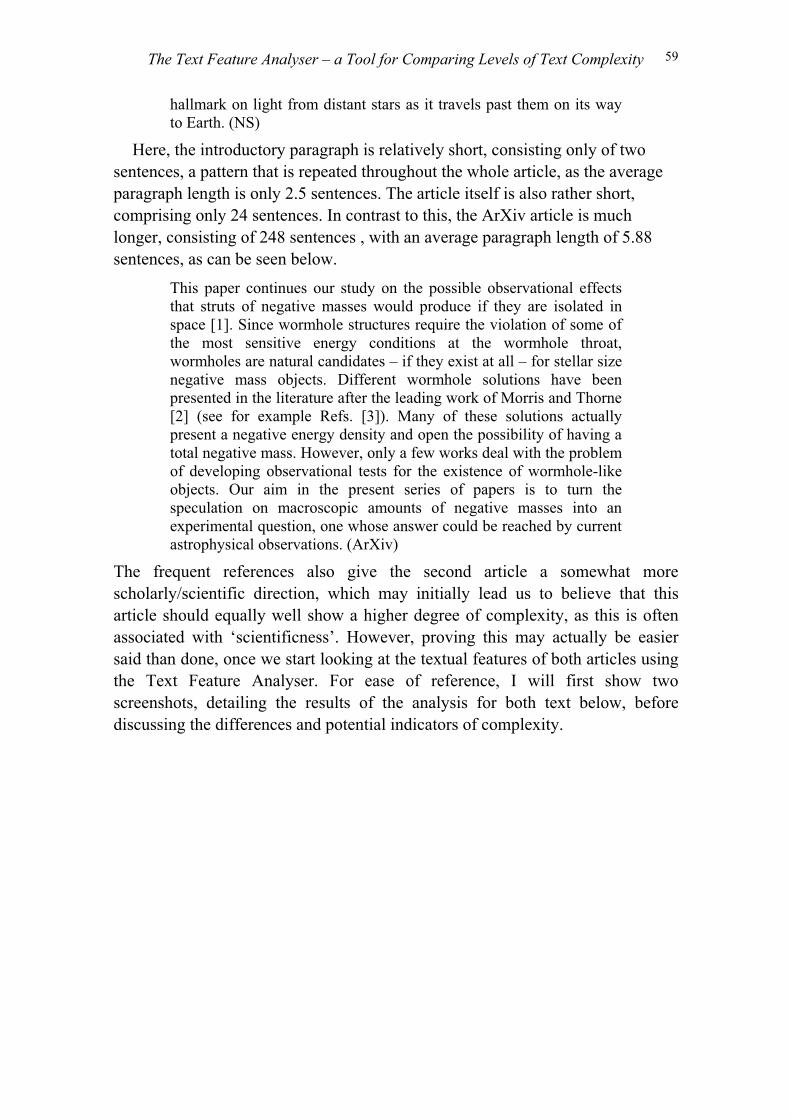
Here, the introductory paragraph is relatively short, consisting only of two

sentences, a pattern that is repeated throughout the whole article, as the average

paragraph length is only 2.5 sentences. The article itself is also rather short,

comprising only 24 sentences. In contrast to this, the ArXiv article is much

longer, consisting of 248 sentences , with an average paragraph length of 5.88

sentences, as can be seen below.

This paper continues our study on the possible observational effects

that struts of negative masses would produce if they are isolated in

space [1]. Since wormhole structures require the violation of some of

the most sensitive energy conditions at the wormhole throat,

wormholes are natural candidates – if they exist at all – for stellar size

negative mass objects. Different wormhole solutions have been

presented in the literature after the leading work of Morris and Thorne

[2] (see for example Refs. [3]). Many of these solutions actually

present a negative energy density and open the possibility of having a

total negative mass. However, only a few works deal with the problem

of developing observational tests for the existence of wormhole-like

objects. Our aim in the present series of papers is to turn the

speculation on macroscopic amounts of negative masses into an

experimental question, one whose answer could be reached by current

astrophysical observations. (ArXiv)

The frequent references also give the second article a somewhat more

scholarly/scientific direction, which may initially lead us to believe that this

article should equally well show a higher degree of complexity, as this is often

associated with ‘scientificness’. However, proving this may actually be easier

said than done, once we start looking at the textual features of both articles using

the Text Feature Analyser. For ease of reference, I will first show two

screenshots, detailing the results of the analysis for both text below, before

discussing the differences and potential indicators of complexity.


60

Fig. 5: Analysis results for the NS text

Fig. 6: Analysis results for the ArXiv article

MARTIN WEISSER

61

Let’s start by discussing the general descriptive statistics. Here, both texts,

apart from their obvious differences in overall and paragraph length, show

surprisingly few differences. As a matter of fact, the values for the FOG and

lexical density indexes are remarkably similar. The latter only seems to indicate

that both texts are – in a sense – more or less equally academic, whereas the

former seems to indicate that theses two texts are actually relatively low on the

‘diffuseness’ scale, with the ArXiv text exhibiting a slightly higher FOG index,

especially once the stop words have been excluded from the calculation.

What seems to be slightly more relevant as a potential indicator of increased

complexity in the ArXiv text is the fact that, although its mean sentence length is

a little lower, possibly due to the relatively high occurrence of equations/formula,

the standard deviation of sentence length is actually higher, perhaps indicating a

higher degree of variability. This also seems to be supported by the lower

type/token ratio, which indicates that the more scientific text uses a higher

number of (low-frequency, content) words, thus making it more diverse, and

possibly more specific.

In order to be able to compare the two texts better in terms of the additional

features, the logical thing to do is to compare the middle columns because they

reflect the average number of each feature per sentence. Here, when looking at

the text-structuring devices – such as commas, different types of parentheticals or

conjunctions – first, we can observe that the ArXiv text employs a far higher

number of commas, but apparently rather fewer subordinating conjunctions than

the NS text. Although a higher use of commas should actually help to create an

increased cohesive effect and often increase readability, the relative lack of

subordinating conjunctions initially seemed to suggest that the information

contained in the ArXiv text was simply more densely structured. As it turned out

however, the initial definition I had used for cohesive markers had simply been

too restrictive, and the text does indeed contain a few more of these, often in the

form of enumerative devices, such as firstly, secondly, etc., so that the

cohesiveness factor does increase a little once some modifications have been

applied to the previous (experimental) categories. The number of co-ordinating

conjunctions in both texts is relatively similar and therefore may not be a good

distinguishing characteristic.

In terms of modality/stance, the NS text quite clearly demonstrates a higher

degree of hedging than the ArXiv one. However, this is more an indicator of

genre differences between the two texts, rather than of complexity, but confirms

the common stereotype that the more scientific a text is, the more factual it tends

to be. Similarly, when looking at the pronoun use, the more populist NS version

also seems to be slightly more involved, inasmuch as the number of first person

pronouns is higher and, conversely, the number of (more factual) third person

pronouns lower.


62

The number of preposition in the NS text is higher, which – together with the

previously noted higher incidence of commas – may indicate that the ArXiv text

is structurally denser, containing more relative clauses or occurrences of

postmodification. Surprisingly, though, the number of nominalisations is

marginally higher in the NS text, although this is commonly assumed to be a

feature of more scientific texts.

In terms of article usage, the occurrence of definite and indefinite articles

seems to be reversed between the two types of ‘genre’. The higher incidence of

definite articles seems to underline the scientificness or factuality of the ArXiv

text, whereas the NS article appears to be less factual.

CONCLUSION

In this article, I have discussed the main motivation behind the creation of the

Text Feature Analyser and the analysis and configuration features it offers so far.

However, the possibilities for textual exploration such a tool offers are not

limited purely to attempts at identifying the individual features that may account

for textual complexity. Through its simple extensibility and customisability, the

tool should also provide an ideal means for exploring the features underlying

different genres, or potentially even a way into learner error analysis, e.g. by

identifying over- or under-use of specific features. For this, especially the

planned new concordancing feature will be of utmost relevance because it will

provide immediate access to features that may strike the user as being obvious

candidates for further analysis. However, because of its interactive nature, the

program should also be suitable for classroom analysis that goes beyond simple

classroom concordancing techniques, and may help to raise learners’ awareness

of complexity in academic writing, as well as exploring argumentative structures,

specific genre features, etc.

NOTES

1 Pre-modification in this case essentially in the form of deictic elements, such as

sentence adverbials.

2 Although the tool actually assumes that the encoding of these files is UTF-8, a

Unicode format. In practice, however, it hardly makes any difference to the user

who is analysing English texts that primarily rely on ASCII characters.

3 http://www.ims.uni-stuttgart.de/projekte/corplex/TreeTagger/DecisionTree

Tagger.html

4 Wormhole. (2007, April 4). In Wikipedia, The Free Encyclopedia. Retrieved

08:17, April 5, 2007, from

http://en.wikipedia.org/w/index.php?title=Wormhole&oldid=120335350

5 http://arxiv.org/

MARTIN WEISSER

63

REFERENCES

Biber, D. (1988). Variation across speech and writing. Cambridge: Cambridge

University Press.

Biber, D. (2006). University language: A corpus-based study of spoken and written

registers. Amsterdam/Philadelphia: John Benjamins.

Clark, J., & Yallop, C. (1995). An introduction to phonetics and phonology. Oxford:

Blackwell.

Ellis, R., & Hopkins, K. (1985). How to succeed in written work and study. London &

Glasgow: Collins.

Friedl, J. (2002). Mastering regular expressions. Beijing, Cambridge, etc.: O’Reilley.

Halliday, M. (1985). Spoken and written English. Geelong, Victoria: Deakin University

Press.

Hyman, L. (1975). Phonology: Theory and analysis. New York: Holt, Rinehart &

Winston.

Ure, J. (1971). Lexical density and register differentiation. In Perren, G., & Trim, J.

(Eds.), Applications of Linguistics: Selected Papers of the 2nd International

Conference of Applied Linguistics, Cambridge 1969. Cambridge: Cambridge

University Press, 443-451.

Ventola, E. (1996). Packing and unpacking of information in academic texts. In:

Ventola, E., & Mauranen, A. (eds.), Academic writing: Intercultural and textual

issues. Amsterdam: John Benjamins,153-194.


The Text Feature Analyser

Documents