ANNALS OF ECONOMICS AND FINANCE 11-2, 277–299 (2010) The Term Structure of Interest Rates in a New Keynesian Model with Time-Varying Macro Volatility * Daniel Burren SIGNAL IDUNA Reinsurance Ltd, Bundesplatz 1, CH-6300 Zug, Switzerland E-mail: [email protected] We show that the New Keynesian sticky price model with a cost-push shock and time-varying volatilities of driving forces can reproduce the behavior of the U.S. yield curve in the post-World War II period. Furthermore, we examine how the yield data affects the estimation of time-varying volatilities. We find that if we omit the cost-push shock, we can get very different estimates of the inflation target volatility depending on whether or not we use yield data in addition to macroeconomic data. Therefore, the cost-push shock is crucial for a good prediction of the yield curve. We finally show that the slope of the yield curve depends negatively on both the volatility of the inflation target and the volatility of the cost-push shock. Key Words : Term structure of interest rates; New Keynesian model; Time- varying volatility. JEL Classification Numbers : E43, E44, E47. 1. INTRODUCTION Recent literature has analyzed dynamic term structure models which are derived from macroeconomic models (Wu, 2005; Hoerdahl and Tristani, 2004). The idea is to combine aggregate demand and supply equations with a monetary policy rule to determine the short term interest rate. Absence of arbitrage is then used to derive the implied model of long-term yields. Within models of this kind, time-varying volatility of macro variables is a candidate explanation for the violation of the expectation hypothesis (Campbell and Shiller, 1991; Singleton, 2006). Besides, it is a stylized fact that volatilities of U.S. macro-aggregates have changed during the post- * The author thanks Klaus Neusser, Gregor B¨ aurle and a referee for useful comments. The views expressed here are those of the author and not necessarily those of SIGNAL IDUNA Reinsurance Ltd. 277 1529-7373/2010 All rights of reproduction in any form reserved.

Welcome message from author
This document is posted to help you gain knowledge. Please leave a comment to let me know what you think about it! Share it to your friends and learn new things together.
Transcript

ANNALS OF ECONOMICS AND FINANCE 11-2, 277–299 (2010)
The Term Structure of Interest Rates in a New Keynesian Model
with Time-Varying Macro Volatility*
Daniel Burren
SIGNAL IDUNA Reinsurance Ltd, Bundesplatz 1, CH-6300 Zug, Switzerland
E-mail: [email protected]
We show that the New Keynesian sticky price model with a cost-push shockand time-varying volatilities of driving forces can reproduce the behavior of theU.S. yield curve in the post-World War II period. Furthermore, we examinehow the yield data affects the estimation of time-varying volatilities. We findthat if we omit the cost-push shock, we can get very different estimates of theinflation target volatility depending on whether or not we use yield data inaddition to macroeconomic data. Therefore, the cost-push shock is crucial fora good prediction of the yield curve. We finally show that the slope of theyield curve depends negatively on both the volatility of the inflation targetand the volatility of the cost-push shock.
Key Words: Term structure of interest rates; New Keynesian model; Time-
varying volatility.
JEL Classification Numbers: E43, E44, E47.
1. INTRODUCTION
Recent literature has analyzed dynamic term structure models whichare derived from macroeconomic models (Wu, 2005; Hoerdahl and Tristani,2004). The idea is to combine aggregate demand and supply equations witha monetary policy rule to determine the short term interest rate. Absenceof arbitrage is then used to derive the implied model of long-term yields.Within models of this kind, time-varying volatility of macro variables isa candidate explanation for the violation of the expectation hypothesis(Campbell and Shiller, 1991; Singleton, 2006). Besides, it is a stylized factthat volatilities of U.S. macro-aggregates have changed during the post-
*The author thanks Klaus Neusser, Gregor Baurle and a referee for useful comments.The views expressed here are those of the author and not necessarily those of SIGNALIDUNA Reinsurance Ltd.
277
1529-7373/2010All rights of reproduction in any form reserved.

278 DANIEL BURREN
WWII period (Justiniano and Primiceri, 2006; Stock and Watson, 2005;McConnell and Perez-Quiros, 2000).
This raises some interesting questions. How are movements in the yieldcurve linked to variations in volatilities of macro variables? For example,in a period in which the volatility of the central bank’s inflation target ishigh, investors might demand a different term premium than in a period inwhich the volatility of the central bank’s inflation target is low. How welldoes a model implied yield curve, as described, fit observed yields? Notethat the cited macroeconomic models assumed homoskedastic shocks anddid not address this question. How does yield data affect the estimates ofvolatilities of stochastic driving forces in a macroeconomic model? If time-varying volatilities of macro variables are to produce a model-implied yieldcurve which fits the observed yield curve well, then the fit of the modelimplied yield curve should not be significantly better if, in the estimation,yield data is used in addition to macro data.
We address these questions within the framework of a simple New Keyne-sian sticky price model. New Keynesian models have become very popularfor monetary policy analysis. They are consistent with optimizing behav-ior by private agents while being simple from a conceptual point of view(Walsh, 2003; Woodford, 2003; Clarida et al. , 1999; McCallum and Nelson,1999). We estimate the model by maximum likelihood. We use a rollingwindow of U.S. post-war data in order to estimate time-varying volatilitiesof shocks. In one estimation, we use only macro data whereas in anotherestimation, we use yield data in addition to macro data. Volatilities esti-mated with macro and yield data are defined as implied volatilities whereasvolatilities estimated solely with macro data are called actual volatilities.
We find that the fit of the model implied yield curve improves substan-tially (by a factor of 1.4) when the model is estimated with yield data.It appears that a simple New Keynesian model with time-varying actualvolatilities (i.e. estimated only with macro data) is not rich enough tocapture movements in yields. Since we find that the volatility of the in-flation target is much lower when estimated with yield data than whenestimated without, we deduce that the New Phillips curve in the modelshould be modified. Indeed, adding a cost-push shock to the New Phillipscurve improves the fit of the model implied yield curve by a factor of2.2. Furthermore, the model-implied yield curve turns out to improve onlymarginally if we use yield data in the estimation. Besides, the gap betweenimplied volatility and actual volatility of the inflation target shock has be-come smaller. We explain this finding as follows. In the model withoutthe cost-push shock, the actual volatility of the inflation target is driven byobserved inflation. Therefore, this model does not have the required degreeof freedom for a well fitting yield curve. In the model with the cost-pushshock, however, it is the volatility of the cost-push shock which describes
THE TERM STRUCTURE OF INTEREST RATES 279
the volatility of observed inflation. Thus, the volatility of the inflation tar-get is left over to produce a well fitting yield curve. Therefore, we concludethat a New Keynesian sticky price model with a cost-push shock and time-varying actual volatilities (i.e. estimated without yield data) succeeds inreproducing movements in the term structure of interest rates. Besides, weshow that the slope of the model implied yield curve is negatively relatedto the volatility of the inflation target and to that of the cost-push shock.
In related work (Doh, 2007), the yield curve is used to infer the centralbank’s inflation target in a New Keynesian sticky price model. The noveltyof our paper is the focus on time-varying volatilities and on the fit of themodel implied yield curve. Another difference is the estimation method.In the cited work, the entire model has been estimated using Bayesianmethods.
This paper is organized as follows. Section 2 reviews the Keynesian stickyprice model. Section 3 shows how the yield curve is obtained. Section4 presents the estimation method and Section 5 the results. Section 6concludes the paper.
2. A BENCHMARK NEW KEYNESIAN MODEL
We assume that the economy is of the sticky-price type (Walsh, 2003;Woodford, 2003; Clarida et al. , 1999; McCallum and Nelson, 1999; Gali,2003). In this section, we briefly review the main equations of the model.
2.1. Households
The representative household chooses a consumption path (Cj)j≥t anda labor path (Nj)j≥t in order to maximize expected life-time utility givenby
Et
∞∑
j=t
βjU(Cj , Nj).
Ct is a composite consumption good which consists of differentiated prod-ucts Ct(i) produced by monopolistic competitive firms. It is defined by
Ct =
[∫ 1
0
Ct(i)1− 1
ǫ di
]
ǫ
ǫ−1
, ǫ > 1.
The parameter ǫ governs the price elasticity of demand for the individualgoods. The optimal allocation of expenditures is given by
Ct(i) =
(
Pt(i)
Pt
)−ǫ
Ct (1)
280 DANIEL BURREN
where Pt(i) is the price of good i and Pt is a consumption goods price indexdefined by
Pt =
[∫ 1
0
Pt(i)1−ǫdi
]
1
1−ǫ
.
The budget constraint is given by
PtCt +
J∑
τ=1
b(τ, t)Bτ,t ≤
J−1∑
τ=0
b(τ, t)Bτ+1,t−1 +WtNt − Tt,
where b(τ, t) is the price of a bond at time t which expires in τ months,Bτ,t bond holding, Wt the nominal wage, and Tt taxes. The bonds areassumed to be zero coupon bonds which pay one unit of cash at expirationdate t+ τ . Therefore, b(0, t) = 1 for all t.
We assume a utility function which is additively separable in consump-tion and leisure
U(Ct, Nt) =(Ct/At)
1−ν
1 − ν−N1+ϕt
1 + ϕ,
where At is an exogenous labor-augmenting technological change (Solow,1956) and ν and ϕ are positive real numbers. The dependency of the utilityon the ratio Ct/At, and not on Ct, is not standard. We see it as a simpleway to introduce a feature which has a similar effect as external habitformation (Abel, 1990; Campbell and Cochrane, 1999). That is to say itmakes the coefficient of relative risk aversion time-varying. This coefficientis given by
−CtUcc,tUc,t
= νAt.
Economically, it means that agents dislike situations in which their pro-ductivity is high whereas their consumption is relatively low due to othershocks.
2.2. Firms
On the production side, there is a continuum of monopolistically com-petitive firms, indexed by i. Each firm produces a differentiated good withtechnology
Yt(i) = AtN(i),
where At is the productivity level and N(i) the firm’s labor force. Theabstraction of capital follows literature (McCallum and Nelson, 1999) whichshows that, at least for the United States, there is little relationship between

THE TERM STRUCTURE OF INTEREST RATES 281
the capital stock and output at business-cycle frequencies. The firms faceCalvo-type price stickiness (Calvo, 1983). This is to say that, in eachperiod, some firms are not able to adjust their price. The probability thata firm can adjust the price is given by 1 − θ. Hence, the parameter θ isa measure of the degree of nominal rigidity; a larger θ implies that fewerfirms adjust each period and that the expected time between price changesis longer. The implied average price duration is 1/(1− θ). If a firm adjuststhe price, it does so to maximize the expected discounted value of currentand future profits. Mathematically, this can be expressed as
maxP∗
t(i)
∞∑
j=t
Et
{
θjQt,j(
P ∗t (i)Yj|t(i) −WjNj(i)
)}
,
where Qt,j is the stochastic discount factor of the firms and Yj|t is theproduction of a firm in period j if it could adjust its price in period t. Yj|thas to be equal to the optimal allocation Cj(i) of households given by (1).
The firm sells its goods to private households and to the government.1
Therefore, total demand is given by Ct(i)+Gt(i), where Gt are governmentpurchases. Following extant literature (Gali, 2003), we assume that thegovernment consumes a fraction ςt of each Yt(i).
2.3. Stochastic Driving Forces
The growth rates of technology and of government expenditures followan autoregressive process of order two. They are described by
∆at = µa + ρa,1∆at−1 + ρa,2∆at−2 + σaεat
∆gt = µg + ρg,1∆gt−1 + ρg,2∆gt−2 + σgεgt ,
where ∆ is the first difference operator, at = logAt and gt = − log(1− ςt).We introduced the second lag in order to accommodate potentially higherpersistence in monthly data as compared to quarterly data.
2.4. Flexible Price Equilibrium
In the flexible price equilibrium (θ = 0) firms put a constant commonmarkup on their prices given by ǫ
ǫ−1 . This implies that real marginal costsare constant and equal to minus log ǫ
ǫ−1 = µ for all firms. This leads tothe key equation for finding the flexible price equilibrium:
−µ = wt − pt − at − s,
where wt is the logarithm of the nominal wage, pt = logPt and s a wagesubsidy. Combining this equation with the log-version of the optimality
1Government consumption can be viewed as the sum of usual government expendituresplus net exports (Chari et al. , 2007).

282 DANIEL BURREN
condition − ∂U∂Nt
= ∂U∂Ct
Wt
Pt
,
ϕnt = wt − pt − ν(ct − at),
and with yt = at + nt, provides the solution for yt. Using this solution inthe log-version of the Euler equation,
yt = −1
ν(rt − Et[πt+1] − ρ) + Et[yt+1 − ∆gt+1 − ∆at+1],
gives the solution for the flexible price anticipated real interest rate. Wedenote by yt and rrt the flexible price log-output and the flexible price realinterest rate, respectively. In equilibrium, we have
yt = γ + ψaat + ψggt
rrt = rt − Et[πt+1]
= ρ+ ν(ψa − 1)[µa + ρa,1∆at + ρa,2∆at−1] +
+ν(ψg − 1)[µg + ρg,1∆gt + ρg,2∆gt−2],
where γ = s−µν+ρ , ψa = 1+ν+ϕ
ν+ϕ and ψg = νν+ϕ .2 We assume that γ = 0. This
means that the equilibrium allocation under flexible prices coincides withthe allocation under flexible prices and perfect competition. We recall thatthis is attained by an employment subsidy s which offsets the distortionsassociated with monopolistic competition.
2.5. Monetary Policy
We complete the model with a monetary policy rule of the Taylor type.Concretely, the central bank sets rt according to:
rt = ρrrt−1 + (1 − ρr)(ρ+ π∗t + φπ(Et[πt+1] − π∗
t ) + φyxt) + σrεrt
εrt ∼ iidN(0, 1),
where ρ = ρ+ ν((ψa − 1)µa + (ψg − 1)µg), rt = log{Rt} with Rt denotingthe nominal gross interest rate and π∗
t the central bank’s targeted inflationrate (as given by the logarithm of a price ratio).3 We assume that thetarget π∗
t has a random walk representation:
π∗t = π∗
t−1 + σπεπ∗
t , επ∗
t ∼ iidN(0, 1).
2See Gali (2003) for a derivation with different assumptions on the stochastic drivingforces.
3Taking the logarithm of the price ratio as the inflation rate (target) has an importantadvantage over taking (Pt −Pt−1)/Pt−1: Whereas the latter lies in (−1,∞), the formercan take on any value in R. Therefore, the log-inflation rate is consistent with normallydistributed disturbances. The same applies for rt = log Rt = log{1 + iF F
t }, where iF Ft
stands for the observed federal funds rate.

THE TERM STRUCTURE OF INTEREST RATES 283
2.6. Sticky Price Equilibrium
For the staggered price setting case (θ > 0), the approximate equilibriumconditions are given by
yt = ct + gt (2)
xt = −ν−1(rt − Et[πt+1] − rrt) + Et[xt+1] (3)
πt = βEt[πt+1] + κxt, (4)
where xt = yt − yt is the output gap, πt = log{Pt/Pt−1} the inflationrate and rt the central bank rate. Further, κ = (1 − θ)(1 − βθ)(ν + ϕ)/θ.The monetary policy rule closes the model. The solution is more difficultto obtain than for the flexible price economy. We therefore use a standardalgorithm to derive it (Sims, 2002). This algorithm yields the rationalexpectation solution of the model in the form
ξt = C + Θ0ξt−1 + Θ1εt (5)
where C is a vector of constants and Θ0 and Θ1 are deterministic matricesbuilt up from the structural parameters of the model. ξt is given by
ξt =(
yt yt xt ct gt gt−1 gt−2 at at−1 at−2 rt rrt πt π∗t Etπt+1 Etxt+1 mt ut
)
.
The structural shocks εat , εgt , ε
π∗
t and εrt are stacked in εt.
3. LINKING THE ECONOMY AND THE TERM
STRUCTURE
We obtain the term structure of interest rates from the Euler equation.The Euler equation is given by
b(τ, t) = βEt
[
Uc,t+1/Pt+1
Uc,t/Ptb(τ − 1, t+ 1)
]
= Et[Mt+1b(τ − 1, t+ 1)]. (6)
The stochastic discount factor is well visible in this equation. We define itby
Mt+1 = βUc,t+1/Pt+1
Uc,t/Pt.
Taking logs and using the explicit expression of the utility function, we get
mt+1 = logMt+1 = log β − ν((ct+1 − at+1) − (ct − at)) − πt+1.
Hence, a bond which pays one unit when consumption is higher than pro-ductivity (or when prices are high), costs less than a bond which pays one

284 DANIEL BURREN
unit when consumption is low (or when prices are low). We put mt intoξt in (5). Therefore, the closed form linearized solution of the stochasticdiscount factor is given by the respective line in (5). We write it as
mt+1 = µm + θ′0,mξt + θ′1,mεt+1. (7)
It is well known that if the term structure is inferred by using (5) in thelinearized version of (6), then we would get
log b(τ, t) − log b(τ − 1, t+ 1) = Et[mt+1], (8)
for all τ . This means that ex-ante returns would be equal across bondswith different maturities. In other words, no term premium exists andthe model-implied term structure would be flat. Therefore, this approachis not qualified for the question at hand. One solution consists of doinga second order approximation of the model (Lombardo and Sutherland,2005; Schmitt-Grohe and Uribe, 2004). However, this would substantiallyincrease the computational burden as it requires a particle filter to inferthe likelihood function (Fernandez-Villaverde and Rubio-Ramirez, 2006).Instead, we use a well-known approach (Jermann, 1998). It is based onthe assumption that Mt+1 and b(τ, t) have a log-normal distribution. Thisassumption implies that the Euler equation (6) can then be written as (first,using the moment generating function, then taking logarithms)
log b(τ, t) = Et[mt+1 + log b(τ − 1, t+ 1)] (9)
+1
2V art[mt+1 + log b(τ − 1, t+ 1)].
Thereby, mt+1 is assumed to be given by (7). (9) differs from (8) bya variance-covariance term. This term captures the term premium. Itexpresses that b(τ, t) depends positively on the conditional variances andthe covariance. This introduces heterogeneity in ex-ante return. Evaluating(9) at τ = 1 gives the continuously compounded one period bond return,rt,1 (considering that b(0, t) = 1):
−rt,1 = log(b(1, t)) = Et[mt+1] + (1/2)V art[mt+1]
= µm + θ′0,mξt + (1/2)θ′1,mθ1,m. (10)
In order to determine other bond prices, equation (9) has to be solvedusing the boundary conditions b(0, t) = 1 for all t. The unique solution tothis difference equation is of exponential affine form (Vasicek, 1977; Duffieet al. , 2002) and given by
b(τ, t) = exp (A(τ) +B(τ)′ξt) (11)
THE TERM STRUCTURE OF INTEREST RATES 285
for some functions A and B to be determined. Plugging (11) into thedifference equation (9) verifies that it is indeed a solution. With (7) and(11), (9) can be written as
log b(τ, t) = µm + θ′0,mξt +A(τ − 1) +B(τ − 1)′[C + Θ0ξt]
+2−1V art[θ′1,mεt+1 +B(τ − 1)′Θ1εt+1]
= µm +A(τ − 1) + 2−1θ′1,mθ1,m +B(τ − 1)′(Θ1θ1,m + C)
+2−1B(τ − 1)′Θ1Θ′1B(τ − 1) + (θ′0,m +B(τ − 1)′Θ0)ξt.
Since, by (11), log b(τ, t) has to be equal to A(τ) +B(τ)′ξt, A and B haveto solve the following system of difference equations:
A(τ) = A(τ − 1) + µm + 2−1θ′1,mθ1,m +B(τ − 1)′(Θ1θ1,m + C)
+ 2−1B(τ − 1)′Θ1Θ′1B(τ − 1)
= A(τ − 1) +A(1) +B(τ − 1)′(Θ1θ1,m + C)
+ 2−1B(τ − 1)′Θ1Θ′1B(τ − 1)
B(τ) = θ0,m + Θ′0B(τ − 1)
= B(1) + Θ′0B(τ − 1).
We use the boundary conditions b(0, t) = 1 ∀t to solve these equationsrecursively. The recursion starts with
A(1) = µm + 2−1θ′1,mθ1,m
B(1) = θ0,m.
Given A and B, it is now straightforward to obtain the model impliedterm structure. The continuously compounded yield to maturity t + τ isdefined by
rτ,t = (1/τ)(log(b(0, t+ τ)) − log(b(τ, t)))
= − log(b(τ, t))/τ
= −1
τA(τ) −
1
τB(τ)′ξt. (12)
rτ,t as a function of τ is the model implied term structure. Note that (12)is a multi-factor term structure model where the dynamics of the factorsare obtained from a macro-economic model. This kind of term structuremodels has been discussed (Wu, 2005; Hoerdahl and Tristani, 2004).

286 DANIEL BURREN
3.1. Market Prices of Risk and Time-Varying Term Premium
The expected one-period excess return of holding a bond with maturityt+ τ is defined as
Et[log b(τ − 1, t+ 1)] − log b(τ, t) − r1,t.
Plugging (11) into this equation, gives
Et[log b(τ − 1, t+ 1)] − log b(τ, t) − r1,t = −B(τ − 1)′Θ1θ1,m (13)
−1
2B(τ − 1)′Θ1Θ1B(τ − 1)′.
B(τ − 1)′Θ1 is the coefficient vector which links log b(τ − 1, t+ 1) to εt+1
which is the source of uncertainty between periods t and t+1. It has beenargued that the second term on the right-hand-side is negligible (Wu, 2005).This means that −B(τ−1)′Θ1θ1,m can be interpreted as the compensation,or term premium, of holding B(τ − 1)′Θ1 units of the risks εt+1. Hence,−θ1,m is the vector with the market prices of the risks εt+1. Evaluating(13) successively at (τ, t), (τ − 1, t+ 1),. . ., summing these evaluations andtaking conditional expectations at t leads to
rτ,t =1
τ
τ−1∑
k=0
Et[r1,t+k] + pτ , (14)
where pτ is the term premium built from the right-hand side of (13). Thisequation states that the long term yield equals expected future short termrates plus a premium. This is known as the expectation hypothesis. Ithas been found that (14) is not supported by the data, which has beenattributed to time-varying term premiums (Campbell and Shiller, 1991;Campbell, 1995; Rudebusch and Wu, 2004; Bacchetta et al. , 2009). Inthe present framework, a time-varying term premium may result from ei-ther time-varying structural parameters or from time-varying volatilities.This is the motivation for using the term structure in order to estimatevolatilities.
4. ESTIMATION
4.1. Data and Calibration
We use U.S. macro and treasury bond data, measured at monthly fre-quency in order to estimate the volatilities and the parameters of thestochastic driving forces. The sample period is January 1970 to Septem-ber 2008. We take personal consumption expenditures (PCE), deflated bythe corresponding price index (PCEPI), to measure Ct. We further use the

THE TERM STRUCTURE OF INTEREST RATES 287
price index PCEPI to compute inflation. We proxy Yt with a monthly totalproduction index. For the instrument rt of the central bank we take thefederal funds rate. The bond yields are from Fama CRSP discount bondyield files and Datastream. We use all maturities of one to 13 months andfurther maturities of 24, 25, 36, 37, 48, 49, 60, 61, 84, 85 and 120 months.We obtain the actual volatilities by estimating the model a second timewith macro data only, that is to say with Ct, Yt, the inflation rate andrt. We take extant estimates (Doh, 2007) to calibrate the structural pa-rameters. Since these estimations were done for quarterly data, we makesuitable adaptations (see Table 1). We then estimate the processes of thestochastic shocks in the model. We do another estimation with ν = ϕ = 1and otherwise identical parameters. ν = 1 means that utility is logarithmicin consumption and ϕ = 1 implies a unit wage elasticity of labor supply(Gali, 2003).
TABLE 1.
Calibration of Sticky Price Model
Parameter Calibration 1 Calibration 2
β 0.999 0.999
ν 1.9455 1
ϕ 3.3223 1
ρ 0.001 0.001
ρr 0.4181/3 0.4181/3
φπ 2.034 2.034
φy 0.782 0.782
θ 0.4211/3 0.4211/3
4.2. Econometric Method and Implementation
The system to be estimated is given by
dt = A+Bξt +R wt (15)
ξt+1 = C + Θ0ξt + Θ1εt+1, (16)
where dt contains either the observed macro variables and the yields,
dt =(
yt ct rt πt r1,t r2,t . . . r120,t)
,
or only the macro variables. wt is a standard multivariate normal measure-ment error which we assume to be independent of εt+1. We set R such thatthere are no measurement errors on the macro variables and, if it applies, ameasurement error of 0.0005 on the yields (0.0005 corresponds to 8-10% ofthe average yield). R can be interpreted as a weighting matrix. It allows us

288 DANIEL BURREN
to regulate the importance of yield data in the estimation. The estimationmethod is maximum likelihood. We obtain the likelihood function with theKalman filter. Since direct maximization turned out to have convergenceproblems, we used an EM algorithm (Durbin and Koopman, 2001). Thisalgorithm has two steps, i.e. an expectation evaluation step and a maxi-mization step. We briefly summarize these steps, adapted to the presentproblem. Thereby, ψ denotes the parameter vector to be estimated and dthe vector of all data vectors d1, . . . , dT (idem for ξ).
FIG. 1. Yield Curve Dependency on Volatilities
2040
6080
100120
0.2
0.4
0.6
0.44
0.46
0.48
0.5
0.52
0.54
Maturitiesσπ*
Yie
ld
2040
6080
100120
10
20
30
40
0.1
0.2
0.3
0.4
0.5
Maturitiesσr
Yie
ld
2040
6080
100120
510
1520
25
0.49
0.5
0.51
0.52
0.53
0.54
0.55
Maturitiesσa
Yie
ld
2040
6080
100120
20
40
60
0.44
0.46
0.48
0.5
0.52
0.54
Maturitiesσg
Yie
ld
2040
6080
100120
1
2
3
0.5
0.52
0.54
0.56
0.58
Maturitiesσu
Yie
ld
STEP 1
Let ψ be a trial parameter vector. For this trial value, run the KalmanSmoother to get the smoothed states.

THE TERM STRUCTURE OF INTEREST RATES 289
FIG. 2. Level (solid) and Slope (dashed) of Model Implied Yield Curve
0 10 20 30 400
0.05
0.1
σa
0 20 40 600
0.05
0.1
σg
0 0.2 0.4 0.6 0.8−0.1
0
0.1
σπ*
0 10 20 300
0.2
0.4
σr
0 1 2 30
0.05
0.1
σu
For each macroeconomic state, its arithmetic average over the entire sample pe-
riod (1970-2008) is used. Level and slope of the model implied yield curve at
these averaged states are then computed.
STEP 2
By Bayes rule, the marginal density p of the data given the parameters ψsatisfies
log p(d|ψ) = log p(ξs, d|ψ) − log p(ξs|d, ψ)
= E[log p(ξs, d|ψ)] − E[log p(ξs|d, ψ)],
where E is the expectation operator with respect to density p(ξs|d, ψ) andξs a vector with four linearly independent smoothed states (for example a,g, π∗ and r) as obtained from step 1. Since the economy is driven by fourshocks and since there are no predetermined variables, using more than fourstates would lead to singular covariance matrices. The gradient vector at

290 DANIEL BURREN
FIG. 3. Implied (with term structure) and Actual (without term structure) Volatil-ities
Calibration 1
Inflation Target σπ∗
1975 1980 1985 1990 1995 2000 2005
0.4
0.6
0.8
1
1.2
1.4
1.6
with yieldswithout
Money Shock σr
1975 1980 1985 1990 1995 2000 2005
2
4
6
8
10
12
14
16
with yieldswithout
Calibration 2
Inflation Target σπ∗
1975 1980 1985 1990 1995 2000 2005
0.4
0.6
0.8
1
1.2
1.4
1.6
1.8
with yieldswithout
Money Shock σr
1975 1980 1985 1990 1995 2000 2005
−2
0
2
4
6
8
10
12
14
16
with yieldswithout
the trial value is given by
∂ log p(d|ψ)
∂ψ|ψ=ψ = E
[
∂ log p(ξ, d|ψ)
∂ψ
]
|ψ=ψ
= −1
2
∂
∂ψ
T∑
t=1
(log |RR′| + log |(Θs1)(Θ
s1)
′|
+ (ξst|T − Cs − Θs0ξst−1|T )′((Θs
1)(Θs1)
′)−1(ξst|T − Cs − Θs0ξst−1|T )
(dt −A′ −B′ξt|T )′(RR′)−1(dt −A′ −B′ξt|T ))|ψ=ψ .
Thereby, (Θs1)(Θ
s1)
′ is diagonal with elements σ2a, σ
2g etc. This suggests to
take as a new trial value in step 1 the ψ for which
E
[
∂ log p(ξ, d|ψ)
∂ψ
]
= 0.

THE TERM STRUCTURE OF INTEREST RATES 291
FIG. 4. Implied (with term structure) and Actual (without term structure) Volatil-ities
Calibration 1
Technology Shock σa
1975 1980 1985 1990 1995 2000 2005
0
5
10
15
20
25
with yieldswithout
Government Shock σg
1975 1980 1985 1990 1995 2000 2005
10
15
20
25
30
35
40
with yieldswithout
Calibration 2
Technology Shock σa
1975 1980 1985 1990 1995 2000 2005
10
20
30
40
50
60
70
with yieldswithout
Government Shock σg
1975 1980 1985 1990 1995 2000 2005
0
10
20
30
40
50
with yieldswithout
The first order conditions for σa (σg, σπ and σr are analogous) is
T1
σa−
T∑
t=1
(∆at − ρ1∆at−1 − ρ2∆t−2)2
σ3a
(17)
+T
∑
t=0
∂
∂σa(dt −A′ −B′ξt|T )′(RR′)−1(dt −A′ −B′ξt|T )) = 0.
RR′ is diagonal and can be viewed as a weighing of the yield part: if itsdiagonal elements are very big, then σa is as estimated without yield data.
We assume that the initial states, in step 1, have a diffuse prior density(Durbin and Koopman, 2001). First, we estimate the system for the entiresample period. Then, we take a rolling window of 60 months and estimateonly the volatilities for each window. This is to say that we do not redrawthe states. Instead, we use the filtered states and estimated autocorrela-tions of the shocks from the first estimation. Besides the implied volatilities(as obtained from (17)), we also infer the actual volatilities for each window

292 DANIEL BURREN
by doing the estimation without the yield curve (actual volatility is givenby (17) without the third summand).
5. RESULTS
We first consider how the model implied yield curve depends on thevolatilities (Figures 1 and 2). For this, we evaluate the model at dataaverages and at the estimates obtained from the estimation over the en-tire period with yield-data. We let the volatility of interest vary from itssmallest to its biggest estimate. A first finding is that the volatility of theinflation target negatively influences the slope of the model implied yieldcurve but not its level (the slope being defined as the difference betweenthe yield with the longest maturity and the short term yield, the level asthe unweighted average of the yields over all maturities). The volatility ofthe short term monetary shock, σr, has an effect on both level and slope.The volatilities of the technology shock and of the government shock havea minor effect on level and slopes.
Figures 3 and 4 show actual (estimated without yield data) and implied(estimated with yield data) volatilities with 95% confidence intervals (dot-ted lines) for both calibrations. The implied volatilities of technology andgovernment shocks differ substantially between the two calibrations. Adecay over time is the only thing they appear to have in common. Wefind that implied volatilities of the monetary policy related shocks do notchange a great deal across calibration. Implied volatility of the inflationtarget, however, is significantly lower than actual volatility. We were won-dering whether introducing a first order autocorrelated cost-push shockwould narrow this gap.
A cost-push shock modifies the equilibrium condition for inflation (4) to
πt = βEt[πt+1] + κxt + ut,
where ut = ρuut−1 + σuεut is the cost-push shock (Gali, 2003).
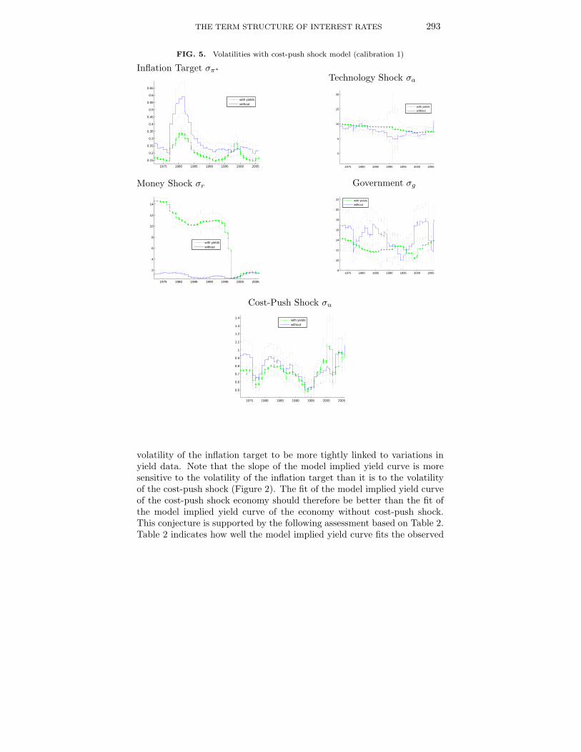
Not surprisingly, it does indeed, as Figure 5 shows (the calibration of theparameters in the model with the cost-push shock is the same as calibrationone). Figure 2 indicates that the volatility of the cost-push shock negativelyaffects the slope of the yield curve.
The cost-push shock volatility resembles the volatility of central bank’sinflation target in Figure 3. Furthermore, both these volatilities resemblethe volatility of the first difference of observed inflation (Figures 6 and 7).This suggests that in the model without the cost-push shock, the volatilityof the inflation target is driven by observed inflation. By contrast, in themodel with cost-push shock it is the volatility of the cost-push shock whichdescribes the volatility of observed inflation. This causes variations in the
THE TERM STRUCTURE OF INTEREST RATES 293
FIG. 5. Volatilities with cost-push shock model (calibration 1)
Inflation Target σπ∗
1975 1980 1985 1990 1995 2000 2005
0.15
0.2
0.25
0.3
0.35
0.4
0.45
0.5
0.55
0.6
0.65
with yieldswithout
Money Shock σr
1975 1980 1985 1990 1995 2000 2005
2
4
6
8
10
12
14
with yieldswithout
Technology Shock σa
1975 1980 1985 1990 1995 2000 2005
0
5
10
15
20
with yieldswithout
Government σg
1975 1980 1985 1990 1995 2000 20058
10
12
14
16
18
20
22
with yieldswithout
Cost-Push Shock σu
1975 1980 1985 1990 1995 2000 2005
0.5
0.6
0.7
0.8
0.9
1
1.1
1.2
1.3
1.4
with yieldswithout
volatility of the inflation target to be more tightly linked to variations inyield data. Note that the slope of the model implied yield curve is moresensitive to the volatility of the inflation target than it is to the volatilityof the cost-push shock (Figure 2). The fit of the model implied yield curveof the cost-push shock economy should therefore be better than the fit ofthe model implied yield curve of the economy without cost-push shock.This conjecture is supported by the following assessment based on Table 2.Table 2 indicates how well the model implied yield curve fits the observed

294 DANIEL BURREN
FIG. 6. ∆πt
1975 1980 1985 1990 1995 2000 2005−0.8
−0.6
−0.4
−0.2
0
0.2
0.4
0.6
FIG. 7. σ(∆πt)
1975 1980 1985 1990 1995 2000 2005
1.2
1.4
1.6
1.8
2
2.2
2.4
2.6
yield curve. The stated numbers are
√
∑
t,τ
(rτ,t − robsτ,t )2,

THE TERM STRUCTURE OF INTEREST RATES 295
FIG. 8. Spread - Calibration 1
1975 1980 1985 1990 1995 2000 2005
−0.2
0
0.2
0.4
Implied Spread (with Term Structure) (solid) and Observed Spread (dashed)
1975 1980 1985 1990 1995 2000 2005
−0.6
−0.4
−0.2
0
0.2
0.4
Implied Spread (without Term Structure) (solid) and Observed Spread (dashed)
1975 1980 1985 1990 1995 2000 2005−0.8
−0.6
−0.4
−0.2
0
0.2
0.4
Difference Implied and Observed Spread
With Term StructureWithout
where rτ,t is the model implied yield as given by (12) and robsτ,t the ob-served yield. The first column specifies where we plug implied and wherewe plug actual volatilities into the model. If nothing else is mentioned,we use actual time-varying volatilities. “σπ∗ implied”, for example, meansthat we use the implied time-varying volatility for the inflation target andactual time-varying volatilities for the other shocks. Not surprisingly, thefit of the model-implied yield curve is better if implied volatilities are used.It improves by a factor of 1.4 or higher (as given by the ratios 12.2/8.7,14.4/10.0,. . . ). Note that the models with constant implied volatilities evenoutperform models with time-varying actual volatilities. For the modelwith a cost-push shock, however, this difference is negligible. We furtherfind that the first calibration provides a better fit than the second calibra-

296 DANIEL BURREN
FIG. 9. Spread - Calibration 2
1975 1980 1985 1990 1995 2000 2005
−0.4
−0.2
0
0.2
0.4
Implied Spread (with Term Structure) (solid) and Observed Spread (dashed)
1975 1980 1985 1990 1995 2000 2005
−0.8
−0.6
−0.4
−0.2
0
0.2
0.4
Implied Spread (without Term Structure) (solid) and Observed Spread (dashed)
1975 1980 1985 1990 1995 2000 2005
−0.8
−0.6
−0.4
−0.2
0
0.2
0.4
Difference Implied and Observed Spread
With Term StructureWithout
tion. Both calibrations, however, perform less well than the economy witha cost-push shock. The fit of the model with a cost-push shock is betterby a factor of 2.2 or higher (leaving out the case constant actual volatili-ties). This confirms our previous conjecture. In a model without cost-pushshock, the volatility of inflation target has to explain the volatility of ob-served inflation and can therefore not help to improve the fit of the impliedterm structure.
In addition, we have observed the following. It does not appear to matterwhether we use implied or actual volatility for technology and/or govern-ment or the cost-push shock. However, we obtain a better fit if we useimplied volatilities solely for the monetary policy related shocks.
Figures 8, 9 and 10 reflect the contents of Table 2. They compare themodel implied yield slope with the observed term spread. The model im-plied slope turns out to be lower than the observed slope. This under-estimation is obviously less pronounced if we use implied instead of the

THE TERM STRUCTURE OF INTEREST RATES 297
FIG. 10. Spread - Cost-Push Shock
1975 1980 1985 1990 1995 2000 2005
−0.4
−0.2
0
0.2
0.4
Implied Spread (with Term Structure) (solid) and Observed Spread (dashed)
1975 1980 1985 1990 1995 2000 2005
−0.4
−0.2
0
0.2
0.4
Implied Spread (without Term Structure) (solid) and Observed Spread (dashed)
1975 1980 1985 1990 1995 2000 2005
−0.5
−0.4
−0.3
−0.2
−0.1
0
0.1
Difference Implied and Observed Spread
With Term StructureWithout
actual volatilities. More interestingly, in the cost-push economy the slopeis quite well estimated independent of whether implied or actual volatilitiesare used.
6. CONCLUSION
We used yield curve data to estimate volatilities of structural shocks in abenchmark sticky price model. We assessed time-variation of the volatilitieswith a rolling data window of 60 months. We found that the sticky pricemodel with a cost-push shock and time-varying actual volatilities, thatis to say estimated solely with macro data, reproduced well the behaviorof observed U.S. zero coupon bond yields. Without the cost-push shock,the fit was less satisfactory. This was reflected by the differences betweenimplied and actual volatilities. In future research, more detailed modelscould be considered. An aim could be to relate the cost-push shock tostructural explanations.

298 DANIEL BURREN
TABLE 2.
Square Root of Sum of Squared Differences Observed - Implied Yields
Volatility Calibration 1 Calibration 2 Cost-push Shock
Constant actual volatilities 29.9 25.3 24.6
Constant implied volatilities 9.8 10.8 4.3
Varying actual volatilities 12.2 14.4 4.4
Varying implied volatilities 8.7 10.0 4.0
σπ∗ implied 9.6 10.5 4.3
σr implied 12.2 14.3 4.1
σa implied 12.2 14.5 4.4
σg implied 11.7 14.3 4.4
σπ∗ , σr implied 9.6 10.3 4.0
σa, σg implied 11.7 14.5 4.4
σu implied - - 4.4
σπ∗ , σr, σu implied - - 4.0
REFERENCES
Abel, Andrew B. 1990. Asset Prices under Habit Formation and Catching Up with theJones. American Economic Review Paper and Proceedings, 80, 38–42.
Bacchetta, Philippe, Mertens, Elmar, and van Wincoop, Eric. 2009. Predictability inFinancial Markets: What Do Survey Expectations Tell Us? Journal of International
Money and Finance, 406–426.
Calvo, G. 1983. Staggered Prices in a Utility-maximizing Framework. Journal of Mon-
etary Economics, 12, 383–398.
Campbell, John Y. 1995. Some Lessons from the Yield Curve. Journal of Economic
Perspectives, 129–152.
Campbell, John Y., and Cochrane, John H. 1999. By force of habit: A consumption-based explanation of aggregate stock market behavior. Journal of Political Economy,205–51.
Campbell, John Y., and Shiller, Robert J. 1991. Yield Spreads and Interest Rate Move-ments: A Bird’s Eye View. Review of Economic Studies, 495–514.
Chari, V.V., Kehoe, Patrick J., and McGrattan, Ellen R. 2007. Business Cycle Account-ing. Econometrica, 75, 782–836.
Clarida, Richard, Galı, Jordi, and Gertler, Mark. 1999. The Science of Monetary Policy:A New Keynesian Perspective. Journal of Economic Literature, 37(4), 1661–1707.
Doh, Taeyoung. 2007. What does the Yield Curve Tell Us About the Federal Reserve’simplicit Inflation Target? Federal Reserve of Kansas City Working Paper.
Duffie, D., Filipovic, D., and Schachermayer, W. 2003. Affine Processes and Applicationsin Finance. The Annals of Applied Probability, 984-1053.
Durbin, J., and Koopman, S.J. 2001. Time Series Analysis by State Space Methods.Oxford University Press New York.
Fernandez-Villaverde, Jesus, and Rubio-Ramirez, Juan F. 2006. Estimating Macroeco-nomic Models: A Likelihood Approach. NBER Technical Working Paper.

THE TERM STRUCTURE OF INTEREST RATES 299
Gali, Jordi. 2003. New Perspectives on Monetary Policy, Inflation and the BusinessCycle. Advances in Economic Theory, III, 151–197.
Hoerdahl, Peter, and Tristani, Oreste. 2004. A Joint Econometric Model of Macroeco-nomic and Term Structure Dynamics. European Central Bank Working Paper.
Jermann, Urban J. 1998. Asset pricing in production economies. Journal of Monetary
Economics, 257–275.
Justiniano, Alejandro, and Primiceri, Giorgio E. 2006. The Time Varying Volatility ofMacroeconomic Fluctuations. NBER Working Paper.
Lombardo, Giovanni, and Sutherland, Alan. 2005. Computing Second-Order-Accurate
Solutions for Rational Expectation Models using Linear Solution Methods. mimeo.
McCallum, Bennett T., and Nelson, Edward. 1999. An Optimizing IS-LM Specifica-tion for Monetary Policy and Business Cycle Analysis. Journal of Money, Credit and
Banking, 31, 296–316.
McConnell, Margret M., and Perez-Quiros, Gabriel. 2000. Output Fluctuations in theUnited States: What Has Changed Since the Early 1980’s? American Economic Review,90, 1464–1476.
Rudebusch, Glenn D., and Wu, Tao. 2004. The Recent Shift in Term Structure Behaviorfrom a No-Arbitrage Macro-Finance Perspective. Federal Reserve Bank of San Francisco
Working Paper.
Schmitt-Grohe, Stephanie, and Uribe, Martın. 2004. Solving dynamic general equilib-rium models using a second-order approximation to the policy function. Journal of
Economic Dynamics and Control, 28, 755–775.
Sims, Christopher A. 2002. Solving Linear Rational Expectations Models. Computa-
tional Economics, 20, 1–20.
Singleton, Kenneth J. 2006. Empirical Dynamic Asset Pricing. Princeton UniversityPress.
Solow, Robert. 1956. A Contribution to the Theory of Economic Growth. Quarterly
Journal of Economics, 70, 65–94.
Stock, James H., and Watson, Mark W. 2005. Understanding Changes in InternationalBusiness Cycle Dynamics. Journal of the European Economic Association, 2005(5),968–1006.
Vasicek, O. 1977. An Equilibrium Characterization of the Term Structure. Journal of
Financial Economics, 177–188.
Walsh, Carl E. 2003. Monetary Theory and Policy. MIT Press.
Woodford, Michael. 2003. Interest and Prices: Foundations of a Theory of Monetary
Policy. Princeton University Press.
Wu, Tao. 2005. Macro Factors and the Affine Term Structure of Interest Rates. FederalReserve Bank of San Francisco Working Paper Series.
Related Documents