The term structure model of corporate bond yields JIE-MIN HUANG 1 , SU-SHENG WANG 1 , JIE-YONG HUANG 2 1 Shenzhen Graduate School Harbin Institute of Technology Shenzhen University Town in Shenzhen City People’s Republic of China, 086-518055 2 Kaifeng city, Henan Province [email protected]; [email protected]; [email protected] Abstract: - We build the term structure of corporate bond yields with N-factor affine model, and we estimate the parameters by using Kalman filtering. We choose weekly average corporate bond yields data in Shanghai Stock Exchange and Shenzhen Stock Exchange. We find the one-factor model and two-factor model could do one-step forward forecasting well, but the three-factor model could fit the observable data well. Key-Words: - corporate bond; yields; term structure; Kalman filtering 1 Introduction Many scholars research on term structure affine models of bonds. The literatures are as below. Some scholars find the three factor model fits observable data well. Dai, Singleton(2000) [1] analyzes the structural differences and goodness-of-fits of affine term structure models. Some models are good at modeling the conditional correlation, some are good at modeling volatilities of the risk factors. He extends N-factor affine model into N+1-factor affine model. Vasicek (1977) Cox, Ingersoll, and Ross (1985) [2,3]assume instantaneous short rate r(t) is the equation of N-factor state variable Y(t), and r(t)= Y(t), and Y(t) follows Gaussian and square root diffusions. Some scholars extend Markov one factor short rate model, and add in a stochastic long-run mean and a volatility v(t) of r(t), dr(t)=( )dt+ . These models come from bond pricing and interest-rate derivatives. Duffee(2002)[4] considers affine model can’t The authors are grateful for research support from the National Natural Science Foundation of China (71103050); Research Planning Foundation on Humanities and Social Sciences of the Ministry of Education (11YJA790152) ; Planning Foundation on Philosophy and Social Sciences in Shenzhen City (125A002). forecast treasury yields. He thinks assuming yields follow stochastic random walk and forecasting results are good. He considers the models failure for the reason that variation of risk compensation is related with interest-rate volatility. He raises essential affine model, and the model keeps the advantage of standard model, but it makes interest- rate variation independent from interest-rate volatility, and this is important for forecasting future yield. Jong(2000) [22] analyzes term structure affine model combining with time series and cross-section information, and he uses discretization continuous time to do Kalman filtering. He finds the three factors model could fit cross-section and dynamic term structure model. Duffie, Kan(1996) [5] finds yields with fixed maturity follow stochastic volatility multi-parameters Markov diffusion process by using continuous no arbitrage multi- factor model of interest-rate term structure. He uses jump-diffusion to solve interest-rate term structure model. Longstaff and Schwartz(1995) [6] evaluate corporate bonds value which have default risk and interest-rate risk by using simple methods. He finds the relation between default risk and interest-rate has important effect on credit spread. Also, he finds credit spread correlates with interest-rate negatively, and the risky bond duration depends on interest rate. He uses V to represent corporate total asset value, and it follows dynamic variation below: dv= , and is constant, and is WSEAS TRANSACTIONS on SYSTEMS Jie-Min Huang, Su-Sheng Wang, Jie-Yong Huang E-ISSN: 2224-2678 409 Issue 8, Volume 12, August 2013

Welcome message from author
This document is posted to help you gain knowledge. Please leave a comment to let me know what you think about it! Share it to your friends and learn new things together.
Transcript

The term structure model of corporate bond yields
JIE-MIN HUANG1, SU-SHENG WANG
1, JIE-YONG HUANG
2
1Shenzhen Graduate School
Harbin Institute of Technology
Shenzhen University Town in Shenzhen City
People’s Republic of China, 086-518055 2Kaifeng city, Henan Province
[email protected]; [email protected]; [email protected]
Abstract: - We build the term structure of corporate bond yields with N-factor affine model, and we
estimate the parameters by using Kalman filtering. We choose weekly average corporate bond yields
data in Shanghai Stock Exchange and Shenzhen Stock Exchange. We find the one-factor model and
two-factor model could do one-step forward forecasting well, but the three-factor model could fit the
observable data well.
Key-Words: - corporate bond; yields; term structure; Kalman filtering
1 Introduction Many scholars research on term structure affine
models of bonds. The literatures are as below. Some
scholars find the three factor model fits observable
data well. Dai, Singleton(2000) [1] analyzes the
structural differences and goodness-of-fits of affine
term structure models. Some models are good at
modeling the conditional correlation, some are good
at modeling volatilities of the risk factors. He
extends N-factor affine model into N+1-factor affine
model. Vasicek (1977) Cox, Ingersoll, and Ross
(1985) [2,3]assume instantaneous short rate r(t) is
the equation of N-factor state variable Y(t), and
r(t)= Y(t), and Y(t) follows Gaussian and
square root diffusions. Some scholars extend
Markov one factor short rate model, and add in a
stochastic long-run mean and a volatility v(t)
of r(t), dr(t)=( )dt+ . These models
come from bond pricing and interest-rate derivatives.
Duffee(2002)[4] considers affine model can’t The authors are grateful for research support from the
National Natural Science Foundation of China
(71103050); Research Planning Foundation on
Humanities and Social Sciences of the Ministry of
Education (11YJA790152) ; Planning Foundation on
Philosophy and Social Sciences in Shenzhen City
(125A002).
forecast treasury yields. He thinks assuming yields
follow stochastic random walk and forecasting
results are good. He considers the models failure for
the reason that variation of risk compensation is
related with interest-rate volatility. He raises
essential affine model, and the model keeps the
advantage of standard model, but it makes interest-
rate variation independent from interest-rate
volatility, and this is important for forecasting future
yield. Jong(2000) [22] analyzes term structure affine
model combining with time series and cross-section
information, and he uses discretization continuous
time to do Kalman filtering. He finds the three
factors model could fit cross-section and dynamic
term structure model. Duffie, Kan(1996) [5] finds
yields with fixed maturity follow stochastic
volatility multi-parameters Markov diffusion
process by using continuous no arbitrage multi-
factor model of interest-rate term structure. He uses
jump-diffusion to solve interest-rate term structure
model. Longstaff and Schwartz(1995) [6] evaluate
corporate bonds value which have default risk and
interest-rate risk by using simple methods. He finds
the relation between default risk and interest-rate
has important effect on credit spread. Also, he finds
credit spread correlates with interest-rate negatively,
and the risky bond duration depends on interest rate.
He uses V to represent corporate total asset value,
and it follows dynamic variation below:
dv= ,and is constant, and is
WSEAS TRANSACTIONS on SYSTEMS Jie-Min Huang, Su-Sheng Wang, Jie-Yong Huang
E-ISSN: 2224-2678 409 Issue 8, Volume 12, August 2013

standard Wiener process. He uses r to represent risk-
free interest rate, and dr=( )dt+ , and
are constant, and is standard Wiener
process, and the correlation of and is .
Cox,Ingersoll and Ross(1985)[2]study intertemporal
interest-rate term structure by using ordinary
equilibrium asset pricing model. In the model,
anticipation, risk aversion, investment choice and
consumption preferences have impact on bond price,
and he provides bond pricing formula and it fits the
data well. Vasicek(1977) [3] assumes: (1)
instantaneous interest rate follows diffusion process;
(2) discount bond price depends on instantaneous
term; (3) market is efficient. He finds bond expected
yields are proportional with standard deviation.
Asileiou(2006) [7]evaluates bond value by using
non-default bond until maturity, and he finds semi-
Markov property holds, and he provides algorithm
for forward transition probability. Lamoureux,
Witte(2002) [8]uses Bayes model to do research. He
finds the three factors model is better.
Some scholars add default factor into bond term
structure model. Duffee(1999) [9]analyzes default
risk in corporate bond price by using term structure
model. He builds square root diffusion transition
process model of corporate instantaneous default
probability, but the model correlates with default
free interest rate. He analyzes time series and cross-
section term structure of corporate bond price by
using extended Kalman filtering. The model fits
corporate bond yields well, and also parameters are
the main factors of yield spread term structure.
Duan and Simonato(1999) [10] build exponent term
structure model for estimating parameters of state
space model. He uses Kalman filtering with the
conditional mean and conditional variance. Duarte
( 2004 ) [11]tries to solve the contradiction in
affine term structure model for fitting mean interest
and interest rate volatility. Dai and Singleton
(2002)[12]find yield curve slope is the linear
function of returns, and this is conflict with
traditional expectation theory. Cheridito, Filipovic
and Kimmel(2007) [13] extend measuring criteria of
market price of affine yield model. His research
could be used into other asset pricing model.
Lando(1998) [14] builds the model of defaultable
security and credit derivative, and it includes market
risk factors and credit risk. He tests how to use term
structure model and price affine model in bonds
with different credit ratings. He analyzes one factor
term structure affine model by using closed method.
Jarrow and Turnbull (1995) [15] provide a new
method for credit risk derivative pricing. There are
two kinds of credit risks, and one is the default risk
in derivatives of basic assets, the other is default risk
of the writer of derivative bonds. Duffee(1998) [16]
considers bond spreads depend on callability of
corporate bond. He tests the assumptions of
investment grade corporate bond. Carr and
Linetsky(2010)[17] take defaultable stock price as
time varying Markov diffusion process with
volatility and default intensity. Dai and
Singleton(2003) [18]observe dynamic term structure
model, and it fits on treasury and swap yield curve,
and default factor follows diffusion, jump diffusion.
Duffie and Lando (2001) [19] study on corporate
bond credit spread term structure with imperfect
information. He assumes bond investors can’t
observe the assets of bond issuers, and they only get
the imperfect accounting reports. He considers
corporate assets follow Geometric Brownian Motion,
and the credit spread has accounting information
character.
Some scholars study term structure model of
commodity future. Schwartz and Smith(2000) [20]
use a two-factor model of commodity prices, and it
allows mean-reversion in short-term prices and
uncertainty in equilibrium level to which prices
revert. They estimate the parameters of the model
using prices for oil futures contracts and then apply
the model to some hypothetical oil-linked assets to
demonstrate its use and some of its advantages over
the Gibson-Schwartz model. Casassus and Collin-
Dufresne(2005)[21] three factor model with
commodity spot prices, convenience yield and
interest rate, and convenience yield relies on spot
price and interest rate, and there is time varying risk
premium. Chen(2009) [23] predicts Taiwan 10-year
government bond yield. Neri(2012) [24]shows how
L-FABS can be applied in a partial knowledge
learning scenario or a full knowledge learning
scenario to approximate financial time series. Neri
(2011) [29] Learns and Predicts Financial Time
Series by Combining Evolutionary Computation and
Agent Simulation. Neri(2012)[30] makes
Quantitative estimation of market sentiment: A
discussion of two alternatives. Wang(2013)[31]
finds Idiosyncratic volatility has an impact on
corporate bond spreads: Empirical evidence from
Chinese bond markets.
In China, Fan longzhen and Zhang guoqing
(2005)[25] analyze time continuous two-factor
generalized Gaussian affine model by using Kalman
filtering. The model could reflect cross-section
characteristic of interest rate term structure, but it
can’t reflect the time series character. Wang
WSEAS TRANSACTIONS on SYSTEMS Jie-Min Huang, Su-Sheng Wang, Jie-Yong Huang
E-ISSN: 2224-2678 410 Issue 8, Volume 12, August 2013

xiaofang, Liu fenggen and Hanlong(2005)[26]
build interest rate term structure curve by using
cubic spline function. Fan longzhe ( 2005 )[27]estimates bond interest rate by using term
structure of yields with three-factor Gaussian
essential affine model. Fan longzhen(2003)[28]
estimates treasury time continuous two factor
Vasicek model by using Kalman filtering. There are
many literatures on interest rate term structure
model, the abroad research focuses on commodity
futures, corporate bond pricing, and some of
corporate bond spread and bond yield. In China,
they are mainly about treasury term structure and
few of corporate bond term structure. We research
on corporate bond yield term structure in Shanghai
and Shenzhen Exchange by using Kalman filtering,
and few scholars has ever researched on it by using
the method, and also we plan to research on the
complex factors on corporate bond spread in
Shanghai and Shenzhen Exchange.
2. Data description We choose corporate bond yields in Shanghai
Exchange and Shenzhen Exchange. We choose
bonds with more than 1 year to maturity, because
bonds with less than 1 year to maturity are very
sensitive to interest rate. We choose corporate bonds
weekly average returns with 3 years, 5 years, 7
years and 10 years maturity from January 1st 2012
to December 31st 2012. The data descriptive
statistics are in table1. We can see the long term
bonds have lower weekly average yields than short
term bonds. According to JB values, only 7 years
bonds don’t follow normal distribution, and others
follow normal distribution.
Table1 descriptive statistics
Y1 Y2 Y3 Y4
Mean 5.6770 5.6300 5.8959 4.2039
Median 5.4073 5.3979 5.7922 4.6498
Max 6.8343 6.8026 6.7393 5.4585
Min 4.8176 4.6666 5.1545 1.4359
St.d 0.6288 0.6465 0.4826 1.0274
skewness 0.6356 0.5716 0.3868 -1.481
kurtosis 2.0264 1.8824 1.9326 4.1198
JB 5.4480 5.4311 3.6929 21.301
P 0.0656 0.0662 0.1578 0.0000
3. Term structure affine model Vasicek (1977) and Cox, Ingersoll and Ross(1985)
assume instantaneous short term interest rate r(t) is
the affine equation of N-factor state vector Y(t). We
assume the equation of r(t) and Y(t) as below:
= (1)
is short term interest rate, is constant and
are the N-state variables which
decide interest rate value. According to short term
interest rate model of Longstaff and Schwartz
(1995), state variables follow mean reversion in the
condition of risk neutral probability.
(2)
The equation is as below:
(3)
Parameters k1, k2, k3,… kn indicate state variables,
and f1t, f2t, f3t, … fnt indicate mean reversion rate,
and , indicate state variables
volatility, and w1t, w2t, w3t, …wnt indicate N
independent Standard Brown Motions. In risk
neutral probability, the unconditional mean of state
variable is 0. denotes long term mean of short
term interest rate in risk neutral probability. In real
probability P, the state variables change as below:
+ +
WSEAS TRANSACTIONS on SYSTEMS Jie-Min Huang, Su-Sheng Wang, Jie-Yong Huang
E-ISSN: 2224-2678 411 Issue 8, Volume 12, August 2013
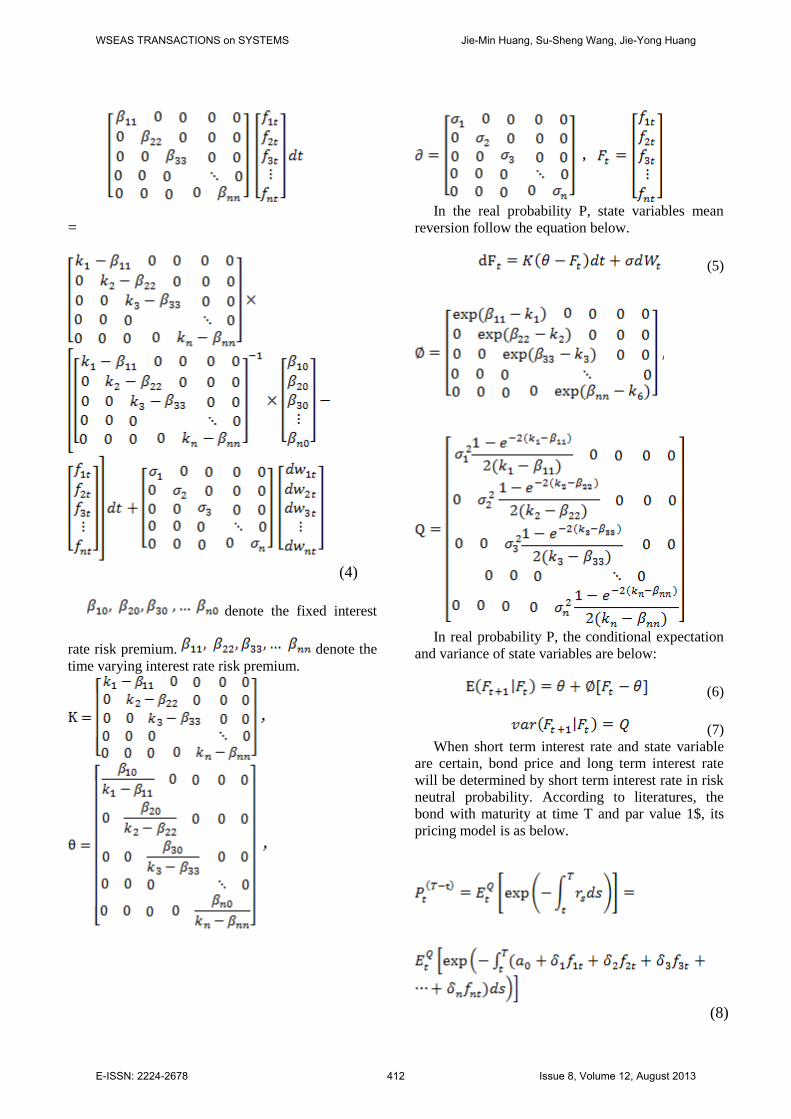
=
(4)
denote the fixed interest
rate risk premium. denote the
time varying interest rate risk premium.
In the real probability P, state variables mean
reversion follow the equation below.
(5)
In real probability P, the conditional expectation
and variance of state variables are below:
(6)
(7)
When short term interest rate and state variable
are certain, bond price and long term interest rate
will be determined by short term interest rate in risk
neutral probability. According to literatures, the
bond with maturity at time T and par value 1$, its
pricing model is as below.
(8)
WSEAS TRANSACTIONS on SYSTEMS Jie-Min Huang, Su-Sheng Wang, Jie-Yong Huang
E-ISSN: 2224-2678 412 Issue 8, Volume 12, August 2013

After derivation, the bond with term , at time t,
the spot interest rate is below:
(9)
4. Kalman filtering
Kalman filtering is made up of recursive
mathematical formulas, and the signal equation
indicates the relation between bond yields
which could be observed and state variables
which can’t be observed. The state equation
indicates the changing process of state variables.
We give initial value for state variable, and we
can estimate the parameters combining with
maximum likelihood estimation model.
According to equation (9), we mark
。
Equation (9) could be written as below:
(10) We choose corporate bond yields data from
Shanghai Exchange and Shenzhen Exchange and the
bonds with maturity of 3 years, 5 years, 7 years and
10 years.
, ,
The signal equation is as below:
(11) According to financial theory, interest rate is
determined by state variables. The mean value of
is 0, and it follows the equation below:
According to (5), we get the state equation below:
(12)
is the stochastic error of state variable, and
its mean value is 0, and its variance is Q. has
initial value and initial variance as below:
WSEAS TRANSACTIONS on SYSTEMS Jie-Min Huang, Su-Sheng Wang, Jie-Yong Huang
E-ISSN: 2224-2678 413 Issue 8, Volume 12, August 2013

The predicting equation of is below:
(13)
The conditional variance of predicting value is
below:
(14)
and follows normal distribution, so the
likelihood equation is below:
(15) The parameters meet the condition below:
In Kalman filtering analysis,
Recursive Algorithm is below:
5. Empirical results analysis
1
2
3
4
5
6
7
5 10 15 20 25 30 35 40 45 50
Y1 Y2 Y3 Y4
Graph1 observable bonds yields
Graph1 indicates corporate bond weekly average
yields in Shanghai Exchange and Shenzhen
Exchange, and Y1 shows corporate bond yields with
3 years maturity, and Y2 shows corporate bond
yields with 5 years maturity, and Y3 shows
corporate bond yields with 7 years maturity, and Y4
means corporate bonds yields with 10 years
maturity. We can see bonds with short term have
higher weekly average yields.
5.1 one-factor empirical analysis With given initial values of parameters, we get
parameters in table2. From table2 we know a0 is
significant at 5% level. is significant at 1%
confidence level, and it means corporate bond yields
fluctuate. is significant at 1% confidence level,
and it means bond yields have mean reversion, but
they reverse slowly. isn’t significant at 1%.
Table2 one-factor affine model results
parameters St.d Z Prob.
a0 3.691** 1.581 2.33 0.0196
0.161*** 0.036 4.50 0.0000
-0.146*** 0.018 --8.24 0.0000
-0.265 0.178 -1.48 0.1377 *** denotes statistical variables are significant at 1%
confidence level and ** denotes statistical variables are
significant at 5% confidence level. From graph2 we can see, it’s one-step forward
forecasting of corporate bond weekly average yields
in Shanghai Exchange and Shenzhen Exchange. The
yields curves in graph2 are similar with the yields
curves in graph1, so the model fits one-step forward
forecasting well. Graph3 indicates the modeling of
real yields in graph1, we can see it can’t fit the real
curve well. So one-factor Kalman filtering model
can’t fit real value well.
WSEAS TRANSACTIONS on SYSTEMS Jie-Min Huang, Su-Sheng Wang, Jie-Yong Huang
E-ISSN: 2224-2678 414 Issue 8, Volume 12, August 2013

Graph2 one-step forward forecasting of yields
-40
-30
-20
-10
0
10
5 10 15 20 25 30 35 40 45 50
Y1F Y2F Y3F Y4F
Graph3 modeling real curve of yields
5.2 Two-factor empirical analysis
From table3 we can see a0 isn’t significant. is
significant at 1% confidence level, and is not
significant, and we infer may be they represent
default risk and liquidity risk. is significant at
1% confidence level, and is not significant.
is significant at 1% confidence level, also is
significant at 1% confidence level, so there are risk
premium in both state variable 1 and state variable 2.
Table3 two-factor affine model results
parameters St.d Z Prob.
a0 1.087 8.948 0.122 0.9033
0.182*** 0.0238 7.664 0.0000
-0.215*** 0.006 -38.93 0.0000
-0.215*** 0.011 -19.86 0.0000
2.330 6.890 0.338 0.7353
1.330 2.495 0.533 0.5941
-4.484*** 1.679 -2.671 0.0076 *** denotes statistical variables are significant on the 1%
confidence level.
From graph4 we can see it’s the one step-forward
forecasting of corporate bond weekly average yields
in Shanghai Exchange and Shenzhen Exchange,
graph4 is similar with graph1, and it means Kalman
filtering two-factor model could forecast yields well.
Graph5 is modeling the real yields, and we can see
graph5 and graph1 is very different, so the two-
factor Kalman filtering model can’t fit real curve
well.
3.6
4.0
4.4
4.8
5.2
5.6
6.0
6.4
6.8
7.2
5 10 15 20 25 30 35 40 45 50
Y1F Y2F Y3F Y4F
Graph4 two-factor one-step forward forecasting
WSEAS TRANSACTIONS on SYSTEMS Jie-Min Huang, Su-Sheng Wang, Jie-Yong Huang
E-ISSN: 2224-2678 415 Issue 8, Volume 12, August 2013

-250
-200
-150
-100
-50
0
50
5 10 15 20 25 30 35 40 45 50
Y1F Y2F Y3F Y4F
Graph5 modeling real curve of yields
5.3 Three-factor empirical analysis
From table4 we can see a0 is significant. is
significant at 1% confidence level, and it means the
state variable 1 fluctuates with time, and isn’t
significant, also isn’t significant. is
significant at 1% confidence level, and it means
state variable 1 follows mean reversion, and is
significant at 5% confidence level, and it means
state variable 2 follows mean reversion, and
, means state variable 2 reverses more
quickly than state variable 1, and is significant
at 1% confidence level, and means state variable 3
follows mean reversion, but it reverses more slowly
than variable2. is significant at 10% confidence
level, and means state variable 1 has time varying
risk premium, and is significant at 5%
confidence level, and means state variable 2 has
time varying risk premium, also is significant
at 1% confidence level, and it means state variable 3
has time varying risk premium, and state variable 2
has the largest time varying risk premium. is
significant at 10% confidence level, and it means
state variable 1 has fixed risk premium, but both
and aren’t significant.
Table4 three-factor affine model results
parameters St.d Z Prob.
a0 3.681 24.374 0.151 0.8800
0.152*** 0.058 2.631 0.0085
-0.229*** 0.072 -3.182 0.0015
-0.635* 0.383 -1.658 0.0974
-0.764 16.977 -0.045 0.9641
0.969** 0.388 2.497 0.0125
0.865** 0.434 1.992 0.0464
0.103 9.854 0.010 0.9917
0.203*** 0.054 3.735 0.0002
0.187*** 0.056 3.367 0.0008
0.976* 0.547 1.787 0.074
1.162 4.954 0.234 0.815
-0.033 2.001 -0.017 0.987 *** denotes statistical variables are significant at the 1%
confidence level. ** denotes statistical variables are significant
at the 5% confidence level. * denotes statistical variables are
significant at 10% confidence level.
WSEAS TRANSACTIONS on SYSTEMS Jie-Min Huang, Su-Sheng Wang, Jie-Yong Huang
E-ISSN: 2224-2678 416 Issue 8, Volume 12, August 2013

-100
-80
-60
-40
-20
0
20
5 10 15 20 25 30 35 40 45 50
Y1F Y2F Y3F Y4F
Graph 6 Three-factor one-step forward forecasting
3.0
3.5
4.0
4.5
5.0
5.5
6.0
6.5
7.0
5 10 15 20 25 30 35 40 45 50
Y1F Y2F Y3F Y4F
Graph 7 modeling real curve of yields
From graph 6 we can see it’s one-step forward
forecasting of average weekly corporate bond yields
in Shanghai Exchange and Shenzhen Exchange, and
it’s very different with graph 1, so the forecasting
isn’t good. Graph 7 is the modeling of real curve,
and it’s similar with graph 1, so the three-factor
model could fit real data well.
6. Conclusion We analyze corporate bond yields term structure in
Shanghai Exchange and Shenzhen Exchange by
using Kalman filtering model. We build N-factor
affine term structure model, and then we use
Kalman filtering to estimate the parameters of one-
factor model, two-factor model and three-factor
model. The results indicate one-factor model and
two-factor model could do one-step forward
forecasting well, and they have fixed risk premium,
but they can’t fit the real data well. Three-factor
model can’t forecast well, but it could fit real data
well, and we add the time varying risk premium
factor into three-factor model, and find they are all
significant, so the three state variables have time
varying risk premium. But only state variable 1 has
the significant fixed risk premium. And the results
are similar with other scholars. I would do further
research on corporate bond spread by using Kalman
filtering.
Reference
[1] Dai Q, Singleton K J, Specification Analysis
of Affine Term Structure Models, The Journal
of finance,Vol. 5, No.4, 2000, pp. 1943-1978.
[2] Vasicek, Oldrich A, An equilibrium
characterization of the term structure, Journal
of Financial Economics, Vol.5, 1977, pp. 177–
188.
[3] Cox, John C., Jonathan E. Ingersoll, Stephen
A. Ross, A theory of the term structure of
interest rates, Econometrica, Vol.53, 1985, pp.
385–408.
[4] Duffee R, Term Premia and Interest Rate
Forecasts in Affine Models, The Journal of
finance, Vol.1, No.6, 2002, pp. 405-443.
[5] Duffie, Kan, A yield-factor model of interest
rates, Mathematical Finance, Vol.4, No.6, 1996,
pp. 379-406.
[6] Longstaff A, Schwartz S, A Simple
Approach to Valuing Risky Fixed and Floating
Rate Debt, The Journal of finance, 1995, Vol.3,
No.3, pp. 789-819.
[7] Vasileiou A, Vasileiou G, An
inhomogeneous semi-markov model for the
term structure of credit risk spreads, Advances
in Applied Probability, Vol.1, No.38, 2006, pp.
171-198.
[8] Lamoureux G, Witte H, Empirical Analysis
of the Yield Curve: The Information in the Data
Viewed through the Window of Cox, Ingersoll,
and Ross, The Journal of finance, Vol.3, No.6,
2002, pp. 1479-1520.
WSEAS TRANSACTIONS on SYSTEMS Jie-Min Huang, Su-Sheng Wang, Jie-Yong Huang
E-ISSN: 2224-2678 417 Issue 8, Volume 12, August 2013

[9] Duffee R, Estimating the Price of Default
Risk, The Review of Financial Studies, Vol.1,
No.12, 1999, pp. 197-226.
[10] Duan, Simonato, Estimating and Testing
Exponential-Affine Term Structure Models by
Kalman Filter, Review of Quantitative Finance
and Accounting, Vol.13, 1999, pp. 111-135.
[11] Duarte, Evaluating an Alternative Risk
Preference in Affine Term Structure Models,
The Review of Financial Studies, Vol.2, No.17,
2004, pp. 379-404.
[12] Dai Q, Singleton K J, Expectation puzzles,
time-varying risk premia, and affine models of
the term structure, Journal of Financial
Economics, Vol.63, 2002, pp. 415-441.
[13] Cheridito, Filipovic, Kimmel L R, Market
price of risk specifications for affine models:
Theory and evidence, Journal of Financial
Economics, Vol.83, 2007,pp. 123-170.
[14] Lando, On Cox Processes and Credit Risky
Securities, Review of Derivatives Research,
Vol.2, 1998, pp. 99-120.
[15] Jarrow A R, Turnbull M S, Pricing
Derivatives on Financial Securities Subject to
Credit Risk, The Journal of finance, Vol.1,
No.5, 1995, pp. 53-85.
[16] Duffee R G. The Relation Between
Treasury Yields and Corporate Bond Yield
Spreads [J]. The Journal of finance, 1998, 6
(53): 2225-2241.
[17] Carr, Linetsky, Time-changed markov
processes in unified credit-equity modeling,
Mathematical Finance, Vol.20, No.4, 2010, pp.
527–569.
[18] Dai, Singleton, Term Structure Dynamics
in Theory and Reality, The Review of Financial
Studies, Vol.16, No.3, 2003, pp. 631-678.
[19] Duffie, Lando, Term structure of credit
spreads with incomplete accounting information,
Econometrica, Vol.69, No.3, 2001, pp. 633-664.
[20] Schwartz, Smith J E, Short-Term
Variations and Long-Term Dynamics in
Commodity Prices, Management Science, Vol.7,
No. 46, 2000, pp.893–911.
[21] Casassus, Collin-Dufresne, Stochastic
Convenience Yield Implied from Commodity
Futures and Interest Rates, The Journal of
finance, Vol.5, 2005,pp. 2283-2331.
[22] Jong D F, Time Series and Cross-section
information in Affine Term-Structure Models,
Journal of Business & Economic Statistics,
Vol.18, No.3, 2000,pp. 300-314. [23] K. Chen; H. Lin; T. Huang, The Prediction of
Taiwan 10-Year Government Bond Yield, WSEAS
Transactions on Systems, Vol.8, No. 9, 2009, pp.
1051-60.
[24] F. Neri, Agent Based Modeling Under Partial
and Full Knowledge Learning Settings to Simulate
Financial Markets, AI Communications, Vol.25,
No.4, 2012, pp. 295-305.
[25] Fan longzhen, Zhang guoqing, Modeling
yield curves in the SSE with two-factor affine
and Gaussian essential affine models, Journal
of Industrial, Vol.19, No.3, 2005, pp. 97-101.
[26] Wang xiaofang, Liu fenggen, Han long,
Formatting the term structure curve of interest
rates of China’s treasury bonds based on cubic
spline functions, Journal of system engineering,
Vol.23, No.6, 2005, pp. 85-89.
[27] Fan longzhen, Modeling the term structure
of yields in the SSE with three-factor Gaussian
essential affine model, Journal of Industrial,
Vol. 1, No.19, 2005, pp. 81-86.
[28] Fan longzhen, Modeling the term structure
of yields in the SSE with two-factor Vasicek
mode, Journal of FUDAN University, Vol. 42,
No.5, 2003, pp. 773-778.
[29] F. Neri, Learning and Predicting Financial
Time Series by Combining Evolutionary
Computation and Agent Simulationm,
Applications of Evolutionary Computation,
LNCS 6625, 2011, pp. 111-119. [30] F. Neri, Quantitative estimation of market
sentiment: A discussion of two alternatives, WSEAS
Transactions on Systems, Vol.11, No.12, 2012, pp.
691-702.
[31] S S Wang, J M huang, Idiosyncratic volatility
has an impact on corporate bond spreads: Empirical
evidence from Chinese bond markets, WSEAS
Transactions on Systems, Vol.12, No.5, 2013, pp.
280-289.
WSEAS TRANSACTIONS on SYSTEMS Jie-Min Huang, Su-Sheng Wang, Jie-Yong Huang
E-ISSN: 2224-2678 418 Issue 8, Volume 12, August 2013
Related Documents