The Taylor Principle and the Taylor Rule Determinacy ...

1

The Taylor Principle and the Taylor Rule Determinacy

Condition in the Baseline New Keynesian

Model: Two Different Kettles of Fish

Tzuhao Huang

The Graduate Center, CUNY

Thom Thurston

Queens College and The Graduate Center, CUNY

Revised June 2012

Abstract

The Taylor Principle (1993) suggests monetary policy should make the interest rate move in

the same direction and by a greater amount than observed movements in inflation. The resulting

co-movements between inflation and the real interest, as Taylor (1999) demonstrated for a simple,

“backward-looking” model, can be shown to be necessary for stability in models of that type. In

the context of the baseline New Keynesian, “forward-looking” model, (NKM) as exposited by

Woodford (2001, 2003) a related “stability and uniqueness” (or determinacy) condition arises

which is necessary for a determinate solution. Woodford and many others have interpreted this

condition as representing the Taylor Principle condition.

In this paper we argue that (1) the dynamic interpretation Woodford and others put on the

NKM determinacy condition is inappropriate; (2) the standard NKM determinacy condition does

not even require (in general) the Taylor Principle (i.e., real interest rate moving together with

inflation) to hold. The Taylor Principle and the NKM determinacy condition are two different

kettles of fish.

2

The Taylor Principle and the Taylor Rule Determinacy

Condition in the Baseline New Keynesian

Model: Two Different Kettles of Fish

I. Introduction

In recent years a great deal of attention among monetary economists has been focused on

the issue of uniqueness, stability and/or “determinacy” in macroeconomic models, particular in

the New Keynesian Model (NKM). Modeling in NKM usually represents monetary policy as

following a Taylor rule, and the parameters of the Taylor rule must meet certain “determinacy

conditions” which may be necessary to rule out both “sunspots” and explosive solutions. At least

since the widely-cited article by Woodford (2001) there has been a consensus that the

determinacy condition in these models is essentially a restatement of the Taylor Principle – that

the policy rule must guarantee that the real interest rate will move together with inflation. This

movement of real interest rates contains demand and inflation responses to shocks that would

otherwise create explosive or stable sunspot solutions. We beg to differ with this line of

reasoning, at least as applied to the NKM.

Our argument is as follows. “Backward-looking” models (such as that by Taylor (1999)

himself) do require the Taylor Principle to hold for “stability” - meaning here where projected

3

paths eventually approach long-run or steady-state solutions of the endogenous variables. But

one should avoid conflating the Taylor Principle with the determinacy condition in the

forward-looking NKM. The determinacy condition in NKM, when met, assures us that the

model’s solution is unique. The dynamics are “stable” in the above sense by construction (all

shocks are AR(1)). If the determinacy condition is not met, the solution is “immediately

explosive” (no finite solution exists) or may result in non-explosive sunspot solutions.1

To illustrate our point, we begin by showing how the two concepts apply in simple,

univariate backward- and forward-looking models. Next we turn to two representative bivariate

(inflation and output gap) backward- and forward-looking models. The backward-looking model

is Taylor’s (1999) model; the forward-looking model is the baseline standard NKM model as

exposited by Clarida, Gali and Gertler (1999), Woodford (2001, 2003) and others. Finally, we

present our most decisive evidence against the view that determinacy requires the Taylor

Principle in NKM models: we provide an example of a NKM-Taylor rule model which is

determinant but the real interest rate moves in the opposite direction of inflation.

4

II. A Univariate Backward-Looking Model

A basic univariate backward-looking model can be written:

(1) �⃖�𝑡 = 𝑎 + 𝑏�⃖�𝑡−1 + 𝑢𝑡, where 𝑢𝑡 = 𝜌𝑢𝑡−1 + 𝜂𝑡 and 0 < 𝜌 < 1. 𝜂t is a white noise.

Iterating the model forward, we rewrite (1) as:

(2) �⃖�𝑡+𝑛 = (1 + 𝑏 + 𝑏2 + ⋯ + 𝑏𝑛)𝑎 + 𝑏𝑛+1�⃖�𝑡−1 + ∑ 𝜌𝑖𝑏𝑛−𝑖𝑛𝑖=0 𝑢𝑡

where n is the number of future periods.2 From equation (2) we see that the dynamics of process

{𝑢𝑡} determine the future path of �⃖�𝑡. Figure 1 illustrates the effects of a positive unit shock

in 𝑢𝑡 on �⃖�𝑡. These paths involve well-defined equilibria for different times. We consider only

positive values of b. Whether b is greater or less than one, the solutions are determinate. The

value of b does determine whether the path is a convergent path or a divergent path. As n

approaches with b<1, the solution path exists and it converges to a certain value.3 As n goes to

infinity with 𝑏 ≥ 1, the solution path still exists but also approaches infinity, i.e., �⃖�𝑡+𝑛 = ∞. The

problem is, for the cases which 𝑏 ≥ 1, the path strays indefinitely from the long-run equilibrium.

This is “instability” in the backward-looking case.

5

III. A Univariate Forward-Looking Model

Contrast this with a forward-looking univariate model such as:

(3) �⃗�𝑡 = 𝑎 + 𝑏𝐸𝑡[�⃗�𝑡+1] + 𝑢𝑡

where 𝑢𝑡 = 𝜌𝑢𝑡−1 + 𝜂𝑡 and 0 < 𝜌 < 1. 𝜂t is a white noise. Again using the iteration method, we

rewrite equation (3) as:

(4) �⃗�𝑡 = (1 + 𝑏 + 𝑏2 + ⋯ + 𝑏𝑛)𝑎 + 𝑏𝑛𝐸𝑡[�⃗�𝑡+𝑛] + (1 + 𝑏𝜌 + 𝑏2𝜌2 + ⋯ 𝑏𝑛𝜌𝑛)𝑢𝑡.4

The necessary condition for convergence in equation (4) is 𝑏 < 1. 𝑏 < 1 guarantees that the

Note: Figure 1 illustrates the effect of a unit shock in 𝑢𝑡 on the path of �⃖�𝑡. When 𝑏 > 1, the

defined future path is unstable and tends toward infinity. When 𝑏 < 1, the defined future path is

stable and the impact of a given shock in 𝑢 heads toward zero

t+i

�⃖� 𝒕

=

t

< 𝜌

> 𝑏 > 𝜌

=

= . 𝟓 = 𝟎. 𝟓

Figure 1. The Dynamics of the Backward-Looking Model with = 𝟎. 𝟓

6

first and second terms of the right hand side of equation (4) have defined limits. If sunspots are

present, they will drop out of the solution. Given the stationary process {𝑢𝑡}, the coefficient of

u has a limit as t goes to infinity. Given this condition, the value of solution paths will follow

(5) �⃗�𝑡 =𝑎

1−𝑏+

1

1−𝑏𝜌𝑢𝑡,

and convergence to this path is immediate. If b >1 and there are no sunspots, the model

explodes instantaneously. If b > 1 and there are sunspots, there may be non-explosive but

arbitrary solutions. Either way, we say the solution is “indeterminate.”

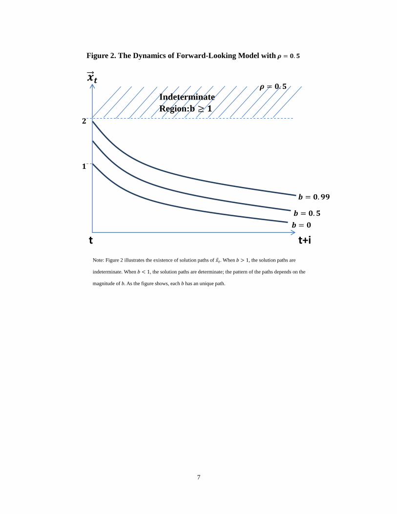
Different values of b (<1) in equation (5) imply different solution paths. Figure 2 illustrates

the dynamics for each unique path with a unit shock in 𝑢𝑡 on �⃗�𝑡. Where a determinate solution

exists, the path is stable (tendency to return to the long-run solution) by construction.

7

Note: Figure 2 illustrates the existence of solution paths of 𝑥𝑡. When 𝑏 > 1, the solution paths are

indeterminate. When 𝑏 < 1, the solution paths are determinate; the pattern of the paths depends on the

magnitude of b. As the figure shows, each b has an unique path.

t+i

𝒙 ⃗ 𝒕

t

Indeterminate

Region: ≥

= 𝟎. 𝟓

Figure 2. The Dynamics of Forward-Looking Model with = 𝟎. 𝟓

= 𝟎. 𝟗𝟗

= 𝟎. 𝟓

= 𝟎

8

IV. Taylor (1999)

Now consider the bivariate (inflation and output) counterparts to univariate models. We start

with the bivariate backward-looking model by Taylor (1999) :

(6) 𝑥𝑡 = 𝛽(𝑖𝑡 𝜋𝑡 𝑟) + 𝑔𝑡

(7) 𝜋t = 𝜋𝑡−1 + 𝛼𝑥𝑡−1 + 𝑢𝑡

(8) 𝑖𝑡 = 𝜑0 + 𝜑𝜋𝜋𝑡 + 𝜑𝑥𝑥𝑡

where x = output gap; 𝜋 = inflation rate; i = short term nominal interest rate. 𝑔 and 𝑢 are

(independent and not auto-correlated) shocks with zero mean. The model parameters 𝛼, 𝛽 are

positive. 𝑟 is the natural rate of interest. 𝜑0, 𝜑𝜋 and 𝜑𝑥 are the policy parameters of the Taylor

rule.

The solution path of inflation can be written as:

(9) 𝜋𝑡+𝑖 = ∑ Λ𝑖−1𝑔𝑡+𝑖𝑛𝑖=1 +

α

1+𝛽𝜑𝑥∑ Λ𝑖−1𝑢𝑡+𝑖

𝑛𝑖=1 + Λ𝑖−1𝜋𝑡 + 𝛼Λ𝑖−1𝑥𝑡

where Λ =𝛼𝛽(1−𝜑𝜋)+(1+𝛽𝜑𝑥)

1+𝛽𝜑𝑥. The key parameter is ˄, which if less than unity will indicate

that projections of πt+n will approach the model’s steady-state value ( ) after

shocks in u or g – hence, the model is “stable” in the sense Taylor intended. . If ˄ > 1, the

model’s projections will depart continuously from steady-state values – “unstable” in the Taylor

sense, though not “explosive” in the immediate sense. Each period’s projection is well-defined.

Since Λ = 1 +𝛼𝛽(1−𝜑𝜋)

1+𝛽𝜑𝑥 the Taylor “stability” condition can be simplified to 𝜑𝜋 >

1.5 This establishes the Taylor Principle and its role in this model.

9

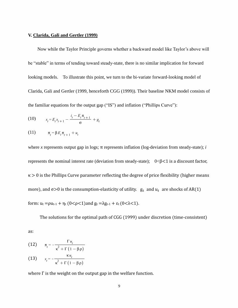
V. Clarida, Gali and Gertler (1999)

Now while the Taylor Principle governs whether a backward model like Taylor’s above will

be “stable” in terms of tending toward steady-state, there is no similar implication for forward

looking models. To illustrate this point, we turn to the bi-variate forward-looking model of

Clarida, Gali and Gertler (1999, henceforth CGG (1999)). Their baseline NKM model consists of

the familiar equations for the output gap (“IS”) and inflation (“Phillips Curve”):

(10)

(11)

where x represents output gap in logs; π represents inflation (log-deviation from steady-state); i

represents the nominal interest rate (deviation from steady-state); 0<β<1 is a discount factor,

κ > 0 is the Phillips Curve parameter reflecting the degree of price flexibility (higher means

more), and σ>0 is the consumption-elasticity of utility. gt and 𝑢𝑡 are shocks of AR(1)

form: ut =ρut-1 + ηt (0<ρ<1)and gt =λgt-1 + εt (0<λ<1).

The solutions for the optimal path of CGG (1999) under discretion (time-consistent)

as:

(12)

(13)

where Γ is the weight on the output gap in the welfare function.

10

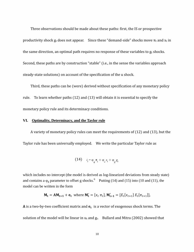
Three observations should be made about these paths: first, the IS or prospective

productivity shock gt does not appear. Since these “demand-side” shocks move πt and xt in

the same direction, an optimal path requires no response of these variables to gt shocks.

Second, these paths are by construction “stable” (i.e., in the sense the variables approach

steady-state solutions) on account of the specification of the u shock.

Third, these paths can be (were) derived without specification of any monetary policy

rule. To learn whether paths (12) and (13) will obtain it is essential to specify the

monetary policy rule and its determinacy conditions.

VI. Optimality, Determinacy, and the Taylor rule

A variety of monetary policy rules can meet the requirements of (12) and (13), but the

Taylor rule has been universally employed. We write the particular Taylor rule as

(14)

which includes no intercept (the model is derived as log-linearized deviations from steady state)

and contains a φg parameter to offset g shocks.6 Putting (14) and (15) into (10 and (11), the

model can be written in the form

𝐌𝐭 = 𝐀𝐌𝐭+ + 𝐞𝐭 where 𝐌𝐭′ = [𝑥𝑡 𝜋𝑡], 𝐌𝐭+

′ = [𝐸𝑡[𝑥𝑡+1] 𝐸𝑡[𝜋𝑡+1]],

A is a two-by-two coefficient matrix and 𝐞𝐭 is a vector of exogenous shock terms. The

solution of the model will be linear in ut and gt. Bullard and Mitra (2002) showed that

11

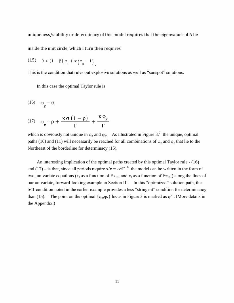
uniqueness/stability or determinacy of this model requires that the eigenvalues of A lie

inside the unit circle, which I turn then requires

(15) .

This is the condition that rules out explosive solutions as well as “sunspot” solutions.

In this case the optimal Taylor rule is

(16)

(17)

which is obviously not unique in φπ and φx. As illustrated in Figure 3,7 the unique, optimal

paths (10) and (11) will necessarily be reached for all combinations of φπ and φx that lie to the

Northeast of the borderline for determinacy (15).

An interesting implication of the optimal paths created by this optimal Taylor rule - (16)

and (17) – is that, since all periods require x/π = -κ/Г 8 the model can be written in the form of

two, univariate equations (xt as a function of Ext+1 and πt as a function of Eπt+1) along the lines of

our univariate, forward-looking example in Section III. In this “optimized” solution path, the

b<1 condition noted in the earlier example provides a less “stringent” condition for determinancy

than (15). The point on the optimal {φπ,φx} locus in Figure 3 is marked as φ’’. (More details in

the Appendix.)

12

VII. Determinate Solutions Without the Taylor Principle

With this background and argument of the previous sections we now return to the classic

interpretation of the NKM-Taylor rule determinacy condition by Woodford (2001, p. 233),

probably the most elegantly expressed and most widely cited:

The determinacy condition…has a simple interpretation. A

feedback rule satisfies the Taylor Principle if it implies that in the

event of a sustained increase in the inflation rate by k percent, the

nominal interest rate will eventually be raised by more than k

Note: 𝜑𝑥′ is the borderline which will meet optimality/time-consistency and make the coefficient on the

future value equals to one. 𝜑𝑥′′ is the borderline where is optimal and meet the standard determinacy

condition ( (𝜑𝜋 1) + (1 𝛽)𝜑𝑥 > 0).

𝜑𝑥

𝜑𝜋

0

Figure 3. The Optimality Taylor Rule and Determinacy Condition

Optimal Loci

( = + ( − )

+

𝒙)

Determinacy

Lower-Bound

𝒙′′ 𝒙

′

13

percent. In the context of the model sketched above, each

percentage point of permanent increase in the inflation rate implies

an increase in the long-run average output gap of 1−β

𝑘 percent; thus

a rule of the form conforms to the Taylor Principle if an only if the

coefficients 𝜑𝜋 and 𝜑𝑥 satisfy 𝜑𝜋 +1−𝛽

𝑘𝜑𝑥 > 1. In particular, the

coefficient values necessarily satisfy the criterion, regardless of the

size of β and k. Thus the kind of feedback prescribed in the Taylor

rule [𝜑𝑥 = 0.5, 𝜑𝜋 = 1.5] suffices to determine an equilibrium

price level.

What is our objection to the statement above? First, the paragraph implies that the

determinacy condition influences the dynamic paths of πt (and presumably xt), whereas we noted

earlier that (15) ensures unique paths for π and x which are reached instantly. Second,

Woodford’s statement suggests that in order for these unique paths to obtain the Taylor Principle

must be apply – i.e., the real interest rate must rise with inflation. It has become nearly universal

to assert that positive co-variation between the real interest rate and inflations critical in avoiding

explosive solutions and sunspots.

It turns out this second suggestion is fairly easy to refute. The standard determinacy

condition (15) does not require the real interest rate to co-vary positively with inflation. We

assume again that gt is offset by the setting (16) ( ). We will not however (for reasons

we will explain in a moment) apply the optimal settings shown in (17). The solutions for πt and xt

will be proportional to ut, which means that the expected t+1 values of these variables can be

14

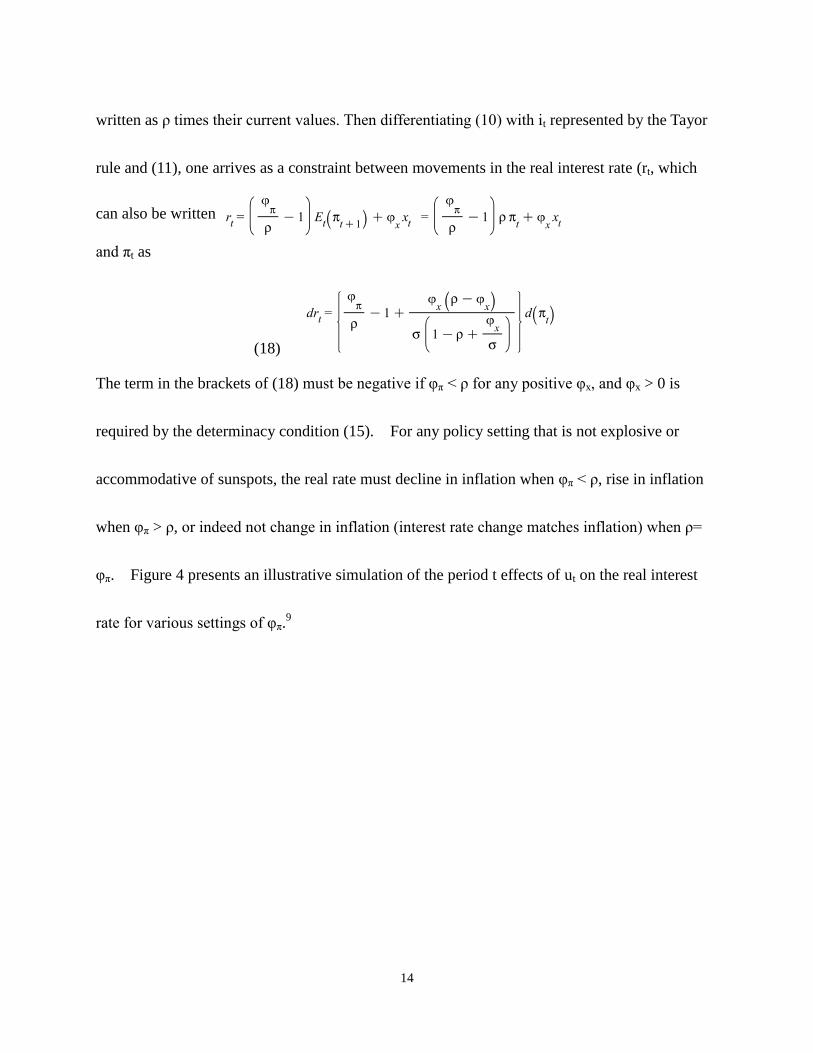
written as ρ times their current values. Then differentiating (10) with it represented by the Tayor

rule and (11), one arrives as a constraint between movements in the real interest rate (rt, which

can also be written

and πt as

(18)

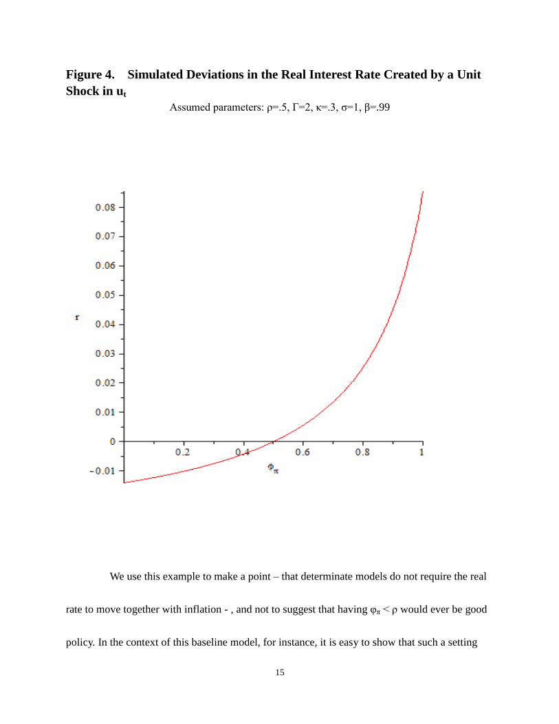
The term in the brackets of (18) must be negative if φπ < ρ for any positive φx, and φx > 0 is

required by the determinacy condition (15). For any policy setting that is not explosive or

accommodative of sunspots, the real rate must decline in inflation when φπ < ρ, rise in inflation

when φπ > ρ, or indeed not change in inflation (interest rate change matches inflation) when ρ=

φπ. Figure 4 presents an illustrative simulation of the period t effects of ut on the real interest

rate for various settings of φπ.9

15

Figure 4. Simulated Deviations in the Real Interest Rate Created by a Unit

Shock in ut

Assumed parameters: ρ=.5, Г=2, κ=.3, σ=1, β=.99

We use this example to make a point – that determinate models do not require the real

rate to move together with inflation - , and not to suggest that having φπ < ρ would ever be good

policy. In the context of this baseline model, for instance, it is easy to show that such a setting

16

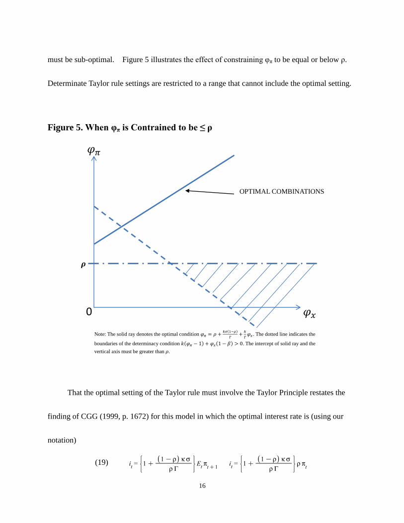
must be sub-optimal. Figure 5 illustrates the effect of constraining φπ to be equal or below ρ.

Determinate Taylor rule settings are restricted to a range that cannot include the optimal setting.

That the optimal setting of the Taylor rule must involve the Taylor Principle restates the

finding of CGG (1999, p. 1672) for this model in which the optimal interest rate is (using our

notation)

(19)

Note: The solid ray denotes the optimal condition 𝜑𝜋 = 𝜌 +𝑘𝜎(1−𝜌)

Γ+

𝑘

Γ𝜑𝑥. The dotted line indicates the

boundaries of the determinacy condition (𝜑𝜋 1) + 𝜑𝑥(1 𝛽) > 0. The intercept of solid ray and the

vertical axis must be greater than 𝜌.

𝜑𝑥

𝜑𝜋

0

Figure 5. When φπ is Contrained to be ≤ ρ

OPTIMAL COMBINATIONS

17

where the term in brackets must be greater than unity. To say that the Taylor Principle should

apply is of course using “should” in the normative sense.

VIII. Summary

The literature has conflated the Taylor Principle with the NKM determinacy condition.

They are two different kettles of fish.

18

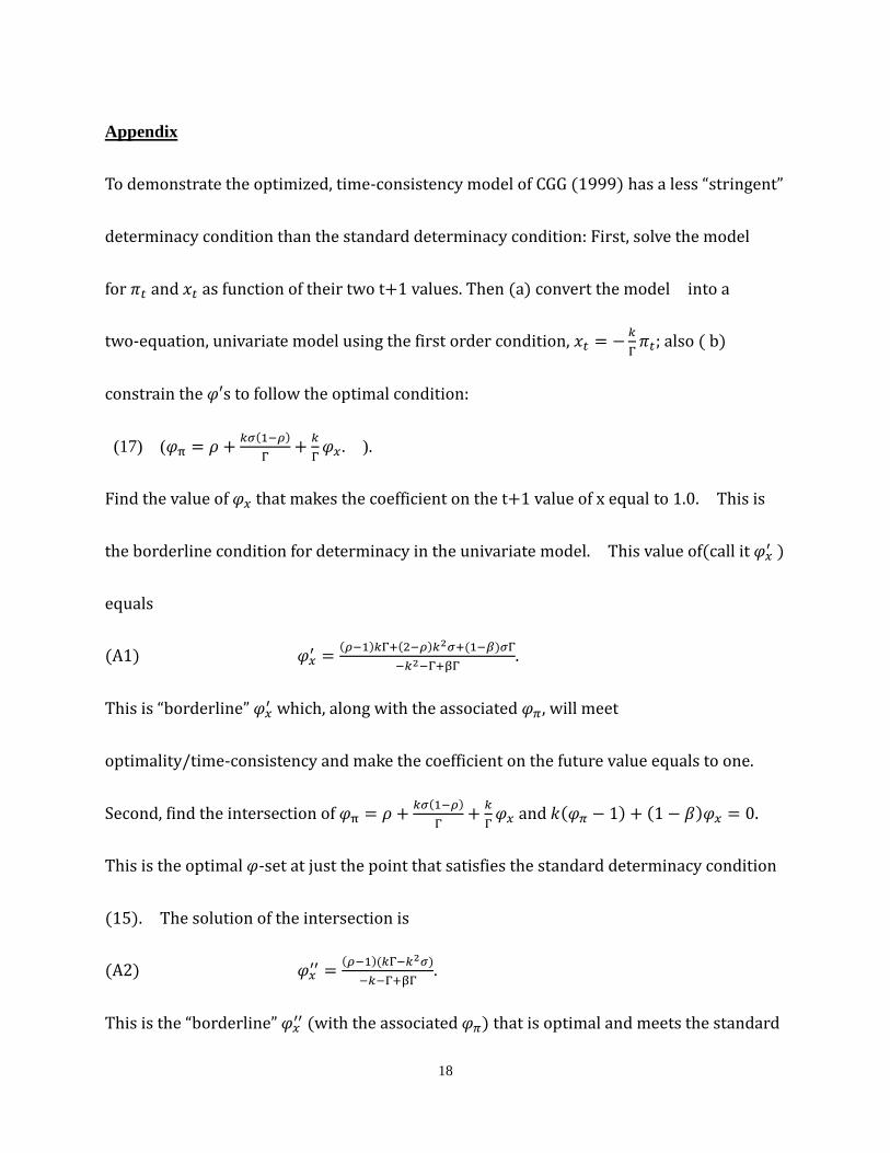
Appendix

To demonstrate the optimized, time-consistency model of CGG (1999) has a less “stringent”

determinacy condition than the standard determinacy condition: First, solve the model

for 𝜋𝑡 and 𝑥𝑡 as function of their two t+1 values. Then (a) convert the model into a

two-equation, univariate model using the first order condition, 𝑥𝑡 = 𝑘

Γ𝜋𝑡; also ( b)

constrain the 𝜑′s to follow the optimal condition:

(17) (𝜑π = 𝜌 +𝑘𝜎(1−𝜌)

Γ+

𝑘

Γ𝜑𝑥. ).

Find the value of 𝜑𝑥 that makes the coefficient on the t+1 value of x equal to 1.0. This is

the borderline condition for determinacy in the univariate model. This value of(call it 𝜑𝑥′ )

equals

(A1) 𝜑𝑥′ =

(𝜌−1)𝑘Γ+(2−𝜌)𝑘2𝜎+(1−𝛽)𝜎Γ

−𝑘2−Γ+βΓ.

This is “borderline” 𝜑𝑥′ which, along with the associated 𝜑𝜋, will meet

optimality/time-consistency and make the coefficient on the future value equals to one.

Second, find the intersection of 𝜑π = 𝜌 +𝑘𝜎(1−𝜌)

Γ+

𝑘

Γ𝜑𝑥 and (𝜑𝜋 1) + (1 𝛽)𝜑𝑥 = 0.

This is the optimal 𝜑-set at just the point that satisfies the standard determinacy condition

(15). The solution of the intersection is

(A2) 𝜑𝑥′′ =

(𝜌−1)(𝑘Γ−𝑘2𝜎)

−𝑘−Γ+βΓ.

This is the “borderline” 𝜑𝑥′′ (with the associated 𝜑𝜋) that is optimal and meets the standard

19

determinacy condition.

Third, subtract (A2) from (A1):

(A3) 𝜑𝑥′′ 𝜑𝑥

′ =−𝑘2𝜎−(1−𝛽)𝜎Γ

−𝑘2−(1−β)Γ.

The value of (A3) is positive given the fact that both numerator and denominator are

negative. That is, φx’ lies inside the standard determinacy region in Figure 3.

20

REFERENCES

Blanchard, Oliver & Charles M. Kahn. 1980. “The Solution of Linear Difference Models under

Rational Expectations.” Econometrica 40(5): 1305-1311

Bullard, James & Kaushik Mitra. 2002. “Learning about Monetary Policy Rules.” Journal of

Monetary Economics 49: 1105-1129

Clarida, Richard, Jordi Gali, Mark Gertler. 1999. “The Science of Monetary Policy: A New

Keynesian Perspective.” Journal of Economic Literature 37(4): 1661-1707

Gali, Jordi. 2008. Monetary Policy, Inflation, and the Business Cycle: An Introduction to the

New Keynesian Framework. Princeton Univ. Press

____________ 2011. “Are Central Bank’s Projections Meaningful?” Journal of Monetary

Economics 58: 537-550

Taylor, John B. 1993. “Discretion versus Policy Rules in Practice.” Carnegie-Rochester

Conference Series on Public Policy 39: 195-214

______________ 1999. “The Robustness and Efficiency of Monetary Policy Rules as Guidelines

for Interest Rate Setting by the European Central Bank.” Journal of Monetary Economics 43:

655-679

Thurston, Thom (2012). “How the Taylor Rule Works in the Baseline New Keynesian Model,”

unpublished.

Walsh, Carl E. (2010). Monetary Theory and Policy, 3rd

Edition, MIT Press

Woodford, Michael. 2001. “The Taylor Rule and Optimal Monetary Policy.” The American

Economic Review 91(2): 232-237

Woodford, Michael. 2003. Interest and Prices: Foundations of a Theory of Monetary Policy.

Princeton Univ. Press.

21

1 This paper does not analyze “sunspot” solutions. These are rational solutions that reflect certain arbitrary and

“non-fundamental” disturbances to expectations which produce self-fulfilling and non-explosive solutions when

mathematical determinacy conditions are not met. When the determinacy conditions are met, the effect is to rule

out ( “cancel out”) the effects of the sunspots. Our focus will be on whether meeting the determinacy conditions has

dynamic implications apart from ruling out sunspots and/or being instantly explosive. We will argue that

determinacy conditions do not have such implications for the baseline New Keynesian Model, notwithstanding

widespread claims they do.

2 When n = 0, equation (2) is the current period. Suppose n = 5, equation (2) expresses that current value of x is

the sum of 5 periods forward, i.e., �⃖�𝑡+5 = (1 + 𝑏 + 𝑏2 + 𝑏3 + 𝑏4 + 𝑏5)𝑎 + 𝑏6�⃖�𝑡−1 + ∑ 𝜌𝑖𝑏5−𝑖5𝑖=0 𝑢𝑡,

where ∑ 𝜌𝑖𝑏5−𝑖5𝑖=0 = 𝑏5 + 𝑏4𝜌 + 𝑏3𝜌2 + 𝑏2𝜌3 + 𝑏𝜌4 + 𝜌5.

3 When 𝑛 → ∞, given 𝑏 < 1, equation (2) converges to �⃖�𝑡+∞ =

𝑎

1−𝑏.

4 𝐸𝑡[𝑢𝑡+1] = 𝑏𝜌𝑢𝑡 , 𝐸𝑡+1[𝑢𝑡+2] = 𝑏2𝜌2𝑢𝑡 and 𝐸𝑡+𝑛−1[𝑢𝑡+𝑛] = 𝑏𝑛𝜌𝑛𝑢𝑡.

5 For Λ < 1,

𝛼𝛽(1−𝜑𝜋)

1+𝛽𝜑𝑥 must be negative. Given positive 𝛼, 𝛽 and 𝜑𝑥, this implies (1 𝜑𝜋) < 0.

6 Woodford (2001) proposes this as a necessary parameter to reach optimality in the baseline NKM with Taylor rule.

7 Assumed parameter values are ρ=.5, Г=2, κ=.3, and σ=1.

8 This is the f.o.c. of the time-consistent “discretionary” solutions of CGG(1999), page 1672.

9 We emphasize that this is not the only set of assumptions that can lead to the real interest rate moving in the

opposite direction of inflation. For example, Thurston (2012) notes conditions in this model that produce a

constant nominal interest rate and a negative co-movement of the real interest rate and inflation.