The Symplectic Geometry of Closed Equilateral Random … · The Symplectic Geometry of Closed Equilateral Random Walks in 3-Space ... (n 3) -tuple of non ... will show that the theory

The Symplectic Geometry of Closed Equilateral Random Walks in 3-Space

Jason Cantarella∗ and Clayton Shonkwiler∗

(Dated: October 22, 2013)

A closed equilateral random walk in 3-space is a selection of unit length vectors giving the steps ofthe walk conditioned on the assumption that the sum of the vectors is zero. The sample space of suchwalks with n edges is the (2n−3)-dimensional Riemannian manifold of equilateral closed polygonsin R3. We study closed random walks using the symplectic geometry of the (2n − 6)-dimensionalquotient of the manifold of polygons by the action of the rotation group SO(3).

The basic objects of study are the moment maps on equilateral random polygon space given by thelengths of any (n−3)-tuple of non-intersecting diagonals. The Atiyah-Guillemin-Sternberg theoremshows that the image of such a moment map is a convex polytope in (n−3)-dimensional space, whilethe Duistermaat-Heckman theorem shows that the pushforward measure on this polytope is Lebesguemeasure on Rn−3. Together, these theorems allow us to define a measure-preserving set of “action-angle” coordinates on the space of closed equilateral polygons. The new coordinate system allows usto make explicit computations of exact expectations for total curvature and for some chord lengths ofclosed (and confined) equilateral random walks, to give statistical criteria for sampling algorithms onthe space of polygons, and to prove that the probability that a randomly chosen equilateral hexagonis unknotted is at least 3/4.

We then use our methods to construct a new Markov chain sampling algorithm for equilateralclosed polygons, with a simple modification to sample (rooted) confined equilateral closed polygons.We prove rigorously that our algorithm converges geometrically to the standard measure on the spaceof closed random walks, give a theory of error estimators for Markov chain Monte Carlo integrationusing our method, and analyze the performance of our method. Our methods also apply to openrandom walks in certain types of confinement, and in general to walks with arbitrary (fixed) edgelengths as well as equilateral walks.

Keywords: closed random walk; statistics on Riemannian manifolds; Duistermaat-Heckman theorem; randomknot; random polygon; crankshaft algorithm

1. INTRODUCTION

In this paper, we consider the classical model of a random walk in R3– the walker chooses eachstep uniformly from the unit sphere. Some of the first results in the theory of these random walksare based on the observation that if a point is distributed uniformly on the surface of a sphere in3-space and we write its’ position in terms of the cylindrical coordinates z and θ, then z and θ areindependent, uniform random variates. This is usually called Archimedes’ Theorem, and it is theunderlying idea in the work of Lord Rayleigh [59], L.R.G. Treloar [68], and many others in the

∗University of Georgia, Mathematics Department, Athens GA

2

theory of random walks, starting at the beginning of the 20th century. In particular, it means thatthe vector of z-coordinates of the edges of a random walk is uniformly distributed on a hypercubeand that the vector of θ-coordinates of the edges is uniformly distributed on the n-torus.

When we condition the walk on closure, it seems that this pleasant structure disappears: theindividual steps in the walk are no longer independent random variates, and there are no obviousuniformly distributed random angles or distances in sight. This makes the study of closed randomwalks considerably more difficult than the study of general random walks. The main point of thispaper is that the apparent disappearance of this structure in the case of closed random walks is onlyan illusion. In fact there is a very similar structure on the space of closed random walks if we arewilling to pay the modest price of identifying walks related by translation and rigid rotation in R3.This structure is less obvious, but just as useful.

As it turns out, Archimedes’ Theorem was generalized in deep and interesting ways in thelater years of the 20th century, being revealed as a special case of the Duistermaat-Heckman theo-rem [25] for toric symplectic manifolds. Further, Kapovich and Millson [37] and Haussmann andKnutson [31] revealed a toric symplectic structure on the quotient of the space of closed equilateralpolygons by the action of the Euclidean group E(3). Together, these theorems define a structureon closed random walk space which is remarkably similar to the structure on the space of openrandom walks: if we view an n-edge closed equilateral walk as the boundary of a triangulatedsurface, we will show below that the lengths of the n − 3 diagonals of the triangulation are uni-formly distributed on the polytope given by the triangle inequalities and that the n − 3 dihedralangles at these diagonals of the triangulated surface are distributed uniformly and independentlyon the (n− 3)-torus. This structure allows us to define a special set of “action-angle” coordinateswhich provide a measure-preserving map from the product of a convex polytope P ⊂ Rn−3 andthe (n− 3)-torus (again, with their standard measures) to a full-measure subset of the Riemannianmanifold of closed polygons of fixed edge lengths.

Understanding this picture allows us to make some new explicit calculations and prove somenew theorems about closed equilateral random walks. For instance, we are able to find an exactformula for the total curvature of closed equilateral polygons, to prove that the expected lengthsof chords skipping various numbers of edges are equal to the coordinates of the center of mass ofa certain polytope, to compute these moments explicitly for random walks with small numbers ofedges, and to give a simple proof that at least 3/4 of equilateral hexagons are unknotted. Further,we will be able to give a unified theory of several interesting problems about confined randomwalks, and to provide some explicit computations of chordlengths for confined walks. We stateupfront that all the methods we use from symplectic geometry are by now entirely standard; the newcontribution of our paper lies in the application of these powerful tools to geometric probability.

We will then turn to sampling for the second half of our paper. Our theory immediately sug-gests a new Markov chain sampling algorithm for confined and unconfined random walks. Wewill show that the theory of hit-and-run sampling on convex polytopes immediately yields a sam-pling algorithm which converges at a geometric rate to the usual probability measure on equilateral

3

closed random walks (or equilateral closed random walks in confinement). Geometric convergenceallows us to apply standard Markov Chain Monte Carlo theory to give error estimators for MCMCintegration over the space of closed equilateral random walks (either confined or unconfined). Oursampling algorithm works for any toric symplectic manifold, so we state the results in generalterms. We do this primarily because various interesting confinement models for random walkshave a natural toric symplectic structure, though our results are presumably applicable far outsidethe theory of random walks. As with the tools we use from symplectic geometry, hit-and-run sam-pling and MCMC error estimators are entirely standard ways to integrate over convex polytopes.Again, our main contribution is to show that these powerful tools apply to closed and confinedrandom walks with fixed edgelengths and to lay out some initial results which follow from theiruse.

2. TORIC SYMPLECTIC MANIFOLDS AND ACTION-ANGLE COORDINATES

We begin with a capsule summary of some relevant ideas from symplectic geometry. A sym-plectic manifold M is an even-dimensional manifold with a special nondegenerate 2-form ω calledthe symplectic form. The volume form dm = 1

n!ωn on M is called the symplectic volume or Liou-

ville volume and the corresponding measure is called symplectic measure. A diffeomorphism of asymplectic manifold which preserves the symplectic form is called a symplectomorphism; it mustpreserve symplectic volume as well. An action of the torus T k on M by symplectomorphismsdefines a moment map µ : M → Rk, where the torus action preserves the fibers (inverse imagesof points) of the map. If the action obeys some mild additional technical hypotheses, it is calledHamiltonian. Two powerful theorems apply in this case: first, the convexity theorem of Atiyah [3]and Guillemin–Sternberg [30] asserts that the image of the moment map is a convex polytope inRk called the moment polytope. The fibers over vertices of the moment polytope consist of fixedpoints of the torus action. Further, if the action is effective, the Duistermaat–Heckman theorem [25]asserts that the pushforward of symplectic measure to the moment polytope is a piecewise polyno-mial multiple of Lesbegue measure. If k = n the symplectic manifold is called a toric symplecticmanifold and the pushforward measure on the moment polytope is a constant multiple of Lebesguemeasure.

If we can invert the moment map, we can construct a map α : P ×Tn →M2n compatible withµ which parametrizes a full-measure subset of M2n by the n coordinates of points in P , which arecalled the “action” variables, and the n angles in Tn, which are called the corresponding “angle”variables. By convention, we call the action variables di and the angle variables θi. We have

Theorem 1 (Duistermaat-Heckman [25]). Suppose M2n is a toric symplectic manifold with mo-ment polytope P , Tn is the n-torus (n copies of the circle) and α inverts the moment map. If wetake the standard measure on the n-torus and the uniform (or Lesbegue) measure on int(P ), thenthe map α : int(P ) × Tn → M2n parametrizing a full-measure subset of M2n in action-angle

4

coordinates is measure-preserving. In particular, if f :M2n → R is any integrable function then∫Mf(x) dm =

∫P×Tn

f(d1, . . . , dn, θ1, . . . , θn) dVolEn ∧dθ1 ∧ · · · ∧ dθn (1)

and if f(d1, . . . , dn, θ1, . . . , θn) = fd(d1, . . . , dn)fθ(θ1, . . . , θn) then∫Mf(x) dm =

∫Pfd(d1, . . . , dn) dVolEn

∫Tn

fθ(θ1, . . . , θn) dθ1 ∧ · · · ∧ dθn. (2)

All this seems forbiddingly abstract, so we give a specific example which will prove importantbelow. The 2-sphere is a symplectic manifold where the symplectic form ω is the ordinary areaform, and the symplectic volume and the Riemannian volume are the same. Any area-preservingmap of the sphere to itself is a symplectomorphism, but we are interested in the action of the circle(or 1-torus) on the sphere given by rotation around the z-axis. This action is by area-preservingmaps, and hence by symplectomorphisms, and in fact it is Hamiltonian. We can see that the actionpreserves the fibers of the moment map, which are just horizontal circles on the sphere. Sincethe dimension of the torus (1) is half the dimension of the sphere (2), the sphere is then a toricsymplectic manifold. The image of the moment map is the closed interval [−1, 1] ⊂ R, which iscertainly a convex polytope. And as the Duistermaat-Heckman theorem claims, the pushforwardof Lebesgue measure on the sphere to this interval is a constant multiple of the Lebesgue measureon the line. This, of course, is just Archimedes’ Theorem, restated in a very sophisticated form.

In particular, it means that one can sample points on the sphere uniformly by choosing theirz and θ coordinates independently from uniform distributions on the interval and the circle. TheDuistermaat-Heckman theorem extends a similar sampling strategy to any toric symplectic mani-fold. The best way to view this sampling strategy, we think, is as a useful technique in the theoryof intrinsic statistics on Riemannian manifolds (cf. [56]) which applies to a special class of man-ifolds. In principle, one can sample the entirety of any Riemannian manifold by choosing chartsfor the manifold explicitly and then sampling appropriate measures on a randomly chosen chart.Since the charts are maps from balls in Euclidean space to the manifold, this reduces the problemto sampling a ball in Rn with an appropriate measure. Of course, this point of view is so generalas to be basically useless in practice: you rarely have explicit charts for a nontrivial manifold, andthe resulting measures on Euclidean space could be very exotic and difficult to sample accurately.

Action-angle coordinates, however, give a single “chart” with a simple measure to sample –the product of Lesbegue measure on the convex moment polytope and the uniform measure on thetorus. There is a small price to pay here. We cannot sample all of the toric symplectic manifoldthis way. The boundary of P corresponds to a sort of skeleton inside the toric symplectic manifoldM , and we cannot sample this skeleton in any very simple way using action-angle coordinates. Ofcourse, if we are using the Riemannian (or symplectic) volume of M to define the probability mea-sure, this is a measure zero subset, so it is irrelevant to theorems in probability. The benefit is thatby deleting this skeleton, we remove most of the topology of M , leaving us with the topologicallyvery simple sample space P × Tn−3.

5

3. TORIC SYMPLECTIC STRUCTURE ON RANDOM WALKS OR POLYGONAL “ARMS”

We now consider the classical space of random walks of fixed step length in R3 and show thatthe arguments underlying the historical application of Archimedes’ theorem (e.g. in Rayleigh [59])can be viewed as arguments about action-angle coordinates on this space as a toric symplecticmanifold. We denote the space of open “arm” polygons with n edges of lengths ~r = (r1, . . . , rn) inR3 by Arm3(n;~r). In particular, the space of equilateral n-edge arms (with unit edges) is denotedArm3(n;~1). If we consider polygons related by a translation to be equivalent, the space Arm3(n;~r)is a product S2(r1) × . . . × S2(rn) of round 2-spheres with radii given by the ri. The standardprobability measure on this space is the product measure on these spheres; this corresponds tochoosing n independent points distributed according to the uniform measure on S2 to be the edgevectors of the polygon.

Proposition 2. The space of fixed edgelength open polygonal “arms” Arm3(n;~r) is the product ofn spheres of radii ~r = (r1, . . . , rn). This is a 2n-dimensional toric symplectic manifold where theHamiltonian torus action is given by rotating each sphere about the z-axis, and the symplectic vol-ume is the standard measure. The moment map µ : Arm3(n;~r)→ Rn is given by the z-coordinateof each edge vector, and the image of this map (the moment polytope) is the hyperbox Πn

i=1[−ri, ri].There is a measure-preserving map

α : Πni=1[−ri, ri]× Tn → Arm3(n;~r).

given explicitly by ~ei = (cos θi√

1− z2i , sin θi

√1− z2

i , zi).

Proof. Recall that the moment polytope is the convex hull of the images of the fixed points ofthe Hamiltonian torus action. The only polygonal arms fixed by the torus action are those whereevery edge is in the ±z-direction, so the z-coordinates of the fixed points are indeed the verticesof the hyperbox Πn

i=1[−ri, ri] and the hyperbox itself is clearly the convex hull. The z-coordinatesz1, . . . , zn and rotation angles θ1, . . . , θn are the action-angle coordinates on Arm3(n;~r) and thefact that α is measure-preserving is an immediate consequence of Theorem 1.

Since we can sample Πni=1[−ri, ri] × Tn directly, this gives a direct sampling algorithm for

(a full-measure subset of) Arm3(n;~r). Of course, direct sampling of fixed-edgelength arms isstraightforward even without symplectic geometry, but this description of arm space has additionalimplications for confinement problems: if we can describe a confinement model by additionallinear constraints on the action variables, this automatically yields a toric symplectic structure onthe space of confined arms. We give examples in the next two sections, then in Section 3.3 weuse this machinery to provide a symplectic explanation for Rayleigh’s formula for the probabilitydensity function (pdf) of the distance between the endpoints of a random equilateral arm.

6

3.1. Slab-Confined arms

One system of linear constraints on the action variables of equilateral arms is the ‘slab’ confine-ment model:

Definition 3. Given a polygon p in R3 with vertices v1, . . . , vn, let zWidth(p) be the maximumabsolute value of the difference between z-coordinates of any two vertices. We define the subspaceSlabArm(n, h) ⊂ Arm3(n;~1) to be the space of equilateral (open) space n-gons up to translationwhich obey the constraint zWidth(p) ≤ h.

This is a slab constraint model where the endpoints of the walk are free (one could also havea model where one or both endpoints are on the walls of the slab). We now rephrase this slabconstraint in action-angle variables.

Proposition 4. A polygon p in Arm3(n;~1) given in action-angle coordinates by(z1, . . . , zn, θ1, . . . , θn) lies in SlabArm(n, h) if and only if the vector ~z = (z1, . . . , zn) ofaction variables lies in the parallelotope P (n, h) given by the inequalities

−1 ≤ zi ≤ 1, −h ≤j∑k=i

zk ≤ h.

Hence, there is a measure-preserving map

α : P (n, h)× Tn → SlabArm(n, h)

given by restricting the action-angle map of Proposition 2.

Proof. This follows directly from Definition 3:∑j

k=i zk is the difference in z-height betweenvertex i and j so this family of linear constraints encodes zWidth(p) ≤ h. The other constraintsjust restate the condition that ~z lies in the moment polytope [−1, 1]n for Arm3(n;~1).

Corollary 5. The probability that a random polygon p ∈ Arm3(n;~1) lies in SlabArm(n, h) isgiven by VolP (n, h)/2n.

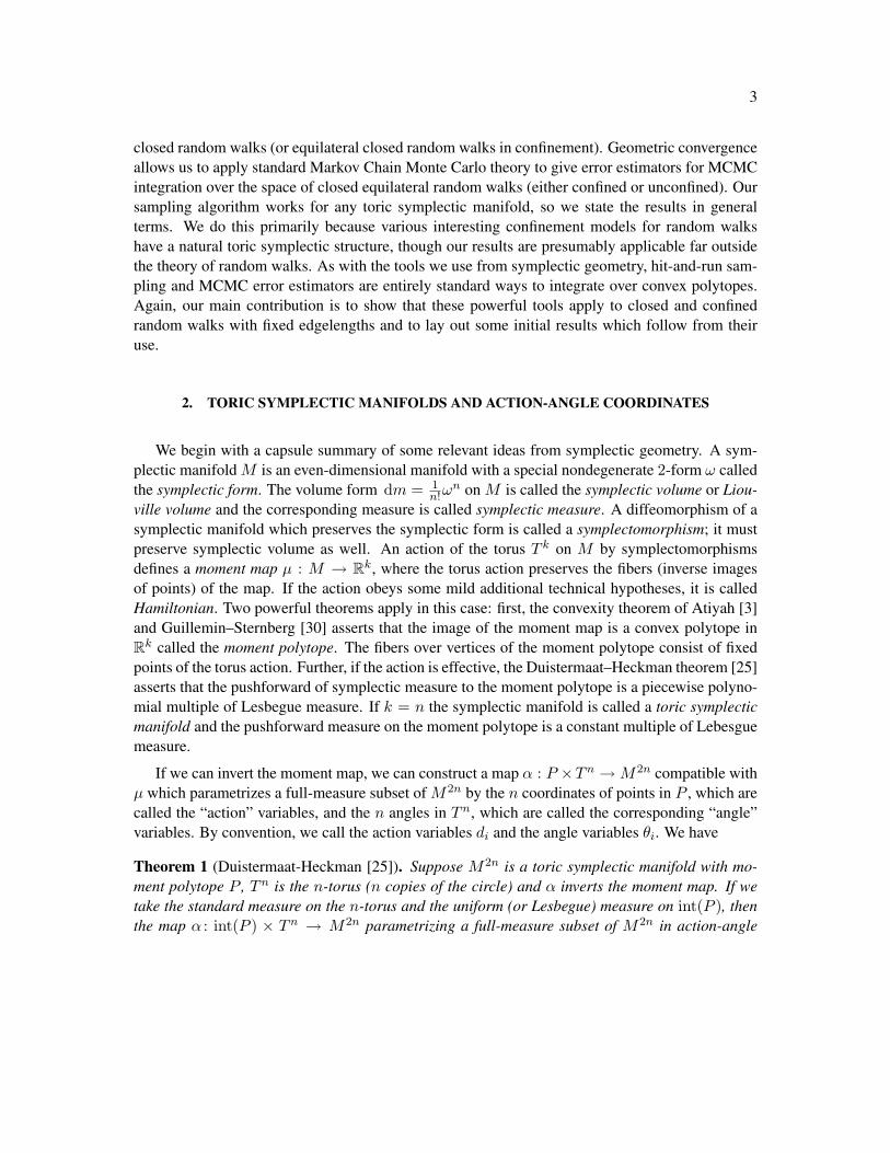
This probability function should be useful in computing the entropic force exerted by an idealpolymer on the walls of a confining slab. Figure 1 shows a collection of these moment polytopesfor different slab widths, and the corresponding volumes.

3.2. Half-space confined arms

A similar problem is this: suppose we have a freely jointed chain which is attached at one endto a plane (which we assume for simplicity is the xy-plane), and must remain in the halfspace on

7

h = 2,Vol = 233 h = 3

2 ,Vol = 15524 h = 1,Vol = 4 h = 1

2 ,Vol = 12

FIG. 1: This figure shows the moment polytopes corresponding to 3-edge arms contained in slabs of widthh as subpolytopes of the cube with vertices (±1,±1,±1), which is the moment polytope for unconfinedarms. In this case, we can compute the volume of these moment polytopes directly using polymake [27].We conclude, for instance, that the probability that a random 3-edge arm is confined in a slab of width 1/2 is1/16.

one side of the plane. This models a polymer where one end of the molecule is bound to a surface(at an unknown site). The moment polytope is

Hn = {~z ∈ [−1, 1]n | z1 ≥ 0, z1 + z2 ≥ 0, . . . , z1 + · · ·+ zn ≥ 0,−1 ≤ zi ≤ 1} (3)

and the analogue of Proposition 4 holds in this case.

We can understand this condition on arms in terms of a standard random walk problem: the ziare i.i.d. steps in a random walk, each selected from the uniform distribution on [−1, 1], and we areinterested in conditioning on the event that all the partial sums are in [0,∞). A good deal is knownabout this problem: for instance, Caravenna gives an asymptotic pdf for the end of a random walkconditioned to stay positive, which is the height of the end of the chain above the plane [17]. If wecould find an explicit form for this pdf, we could analyze the stretching experiment where the freeend of the polymer is raised to a known height above the plane using magnetic or optical tweezers(cf. [65]).

We can directly compute the partition function for this problem; this is the volume of sub-polytope (3) of the hypercube. This result is also stated in a paper of Bernardi, Duplantier, andNadeau [7]. The proof is a pleasant combinatorial argument which is tangential to the rest of thepaper, so we relegate it to Appendix B.

Proposition 6. The volume of the polytope (3) is 12n

(2nn

)= (2n−1)!!

n! .

3.3. Distribution of failure to close lengths

We now apply the action-angle coordinates to give an alternate formula for the pdf of end-to-end distance in a random walk in R3 with fixed step lengths and show that it is equivalent to

8

Rayleigh’s sinc integral formula [59]. This pdf is key to determining the Green’s function for closedpolygons, which in turn is fundamental to the Moore–Grosberg [52] and Diao–Ernst–Montemayor–Ziegler [22–24] sampling algorithms and to expected total curvature calculations [16, 29]. Formathematicians, we note that this pdf is required in order to estimate the entropic elastic forceexerted by an ideal polymer whose ends are held at a fixed distance. Such experiments are actuallydone in biophysics – Wuite et al. [72] (cf. [13]) made one of the first measurements of the elasticityof DNA by stretching a strand of DNA between a bead held in a micropipette and a bead held inan optical trap.

We first establish some lemmas:

Lemma 7. The pdf of a sum of independent uniform random variates in [−r1, r1] to [−rn, rn] isgiven by the pushforward of the Lesbegue measure on Πn

i=1[−ri, ri] to [−∑ri,∑ri] by the linear

function∑xi. This is given by

fn(x) =1

Πni=12ri

1√n

SA(x, r1, . . . , rn), (4)

where SA(x, r1, . . . , rn) is the volume of the slice of the hypercube Πni=1[−ri, ri] by the plane∑

xi = x. The function fn is everywhere n− 2 times differentiable for n > 2.

Proof. This is the coarea formula applied to the hyperbox Πni=1[−ri, ri] and the function

∑xi,

normalized by the volume of Πni=1[−ri, ri]. To see that this function is n− 2 times differentiable,

note that the pdf f2(x) has a corner at x = 0 (and is linear away from this corner) and that we canexpress fn(x) in terms of fn−1 by the convolution integral

fn(x) =∫ rn

−rnfn−1(x− y)

12rn

dy.

where 1/2rn is the pdf of the uniform random variate xn on [−rn, rn].

We have

Proposition 8. The pdf of the end-to-end distance ` ∈ [0,∑ri] over the space of polygonal arms

Arm3(n;~r) is given by

φn(`) =`

2n−1R√n− 1

(SA(`− rn, r1, . . . , rn−1)− SA(`+ rn, r1, . . . , rn−1)) .

where R = Πni=1ri is the product of the edgelengths and SA(x, r1, . . . , rn−1) is the volume of the

slice of the hyperbox Πn−1i=1 [−ri, ri] by the plane

∑n−1i=1 xi = x.

Proof. From our moment polytope picture, we can see immediately that the sum z of the z-coordinates of the edges of a random polygonal arm in Arm3(n;~r) has the pdf of a sum of uniform

9

random variates in [−r1, r1] × · · · × [−rn, rn], or fn(z) in the notation of Lemma 7. Since thisis a projection of the spherically symmetric distribution of end-to-end distance in R3 to the z-axis(R1), Equation 29 of [42] applies1, and tells us that the pdf of ` is given by

φn(`) = −2`f ′n(`).

To differentiate fn(`), we use the following observation (cf. Buonacore [12]):

fn(x) =∫ rn

−rnfn−1(x− y)

12rn

dy =Fn−1(x+ rn)− Fn−1(x− rn)

2rn, (5)

where Fn−1(x) is the cdf of a sum of uniform random variates in [−r1, r1]× · · · × [−rn−1, rn−1].Differentiating and substituting in the results of Lemma 7 yields the formula above.

Since we will often be interested in equilateral polygons with edgelength 1, we observe

Corollary 9. The pdf of the end-to-end distance ` ∈ [0, n] over the space of equilateral armsArm3(n;~1) is given by

φn(`) =`

2n−1√n− 1

(SA(`− 1, [−1, 1]n−1)− SA(`+ 1, [−1, 1]n−1)

). (6)

where SA(x, [−1, 1]n−1) is the volume of the slice of the standard hypercube [−1, 1]n−1 by theplane

∑n−1i=1 xi = x.

The reader who is familiar with the theory of random walks may find the above corollary rathercurious. As mentioned above, the standard formula for this pdf as an integral of sinc functionswas given by Rayleigh in 1919 and it looks nothing like (6). The derivation given by Rayleighof the sinc integral formula has no obvious connection to polyhedral volumes, but in fact by thetime of Rayleigh’s paper a connection between polyhedra and sinc integrals had already beengiven by George Polya in his thesis [57, 58] in 1912. This formula has been rediscovered manytimes [10, 48]. First, we state the Rayleigh formula [23, 59] in our notation:

φn(`) =2`π

∫ ∞0

y sin `y sincn y dy, (7)

where sincx = sinx/x as usual. Now Polya showed that the volume of the central slab of thehypercube [−1, 1]n−1 given by −a0 ≤

∑xi ≤ a0 is given by

Vol(a0) =2na0

π

∫ ∞0

sinc a0y sincn−1 y dy. (8)

1 Lord’s notation can be slightly confusing: in his formula for p3(r) in terms of p1(r), we have to remember that p3(r)is not itself a pdf on the line, it is a pdf on R3. It only becomes a pdf on the line when multiplied by the correctionfactor 4πr2 giving the area of the sphere at radius r in R3.

10

Our SA(x, [−1, 1]n−1) is the (n− 1)-dimensional volume of a face of this slab; since it is this face(and its symmetric copy) which sweep out n-dimensional volume as a0 increases, we can deducethat

SA(x, [−1, 1]n−1) =√n− 12

Vol′(x),

and we can obtain a formula for SA(x, [−1, 1]n−1) by differentiating (8). After some simplifica-tions, we get

SA(x, [−1, 1]n−1) =2n−1

√n− 1π

∫ ∞0

cosxy sincn−1 y dy.

Using the angle addition formula for cos(a+ b), this implies that

SA(`− 1, [−1, 1]n−1)− SA(`+ 1, [−1, 1]n−1) =2n−1

√n− 1π

∫ ∞0

2 sin y sin `y sincn−1 y dy

=2n√n− 1π

∫ ∞0

y sin `y sincn y dy.

Multiplying by the coefficient `2n−1

√n−1

from (6) recovers the Rayleigh form (7) of the pdf φn.

Given (6) and (7), the pdf of the failure-to-close vector ~ =∑~ei with length |~ | = ` can be

written in the following forms:

Φn(~) =1

4π`2φn(`) =

12n+1π`

√n− 1

(SA(`− 1, [−1, 1]n−1)− SA(`+ 1, [−1, 1]n−1)

)=

12π2`

∫ ∞0

y sin `y sincn y dy (9)

The latter formula for the pdf appears in Grosberg and Moore [52] as equation (B5). Since Grosbergand Moore then actually evaluate the integral for the pdf as a finite sum, one immediately suspectsthat there is a similar sum form for the slice volume terms in (6). In fact, we have several optionsto choose from, including using Polya’s finite sum form to express (8) and then differentiating thesum formula with respect to the width of the slab. We instead rely on the following theorem, whichwe have translated to the current situation.

Theorem 10 (Marichal and Mossinghoff [48]). Suppose that ~w ∈ Rn has all nonzero componentsand suppose z is any real number. Then the (n− 1)-dimensional volume of the intersection of thehyperplane 〈~w,~v〉 = z with the hypercube [−1, 1]n is given by

Vol =|~w|2

(n− 1)! Πwi

∑A⊂{1,...,n}

(−1)|A|

z +∑i 6∈A

wi −∑i∈A

wi

n−1

+

, (10)

where |~w|2 is the usual (L2) norm of the vector ~w, and x+ = max(x, 0), and we use the convention00 = 0 when considering the n = 1 case.

11

For our SA(x, [−1, 1]n−1) function, the vector ~w consists of all 1’s, and using the fact that thenumber of subsets of {1, . . . , n} with cardinality k is

(nk

)it follows that

Proposition 11. The n− 2 dimensional volume SA(x, [−1, 1]n−1) is given by the finite sum

SA(x, [−1, 1]n−1) =√n− 1

(n− 2)!

n−1∑k=0

(−1)k(n− 1k

)(x+ n− 1− 2k)n−2

+ . (11)

We can combine this with (9) to obtain the explicit piecewise polynomial pdf for the failure-to-close vector (for n ≥ 2):

Φn(~) =n− 1

2n+1π`

n−1∑k=0

(−1)k

k!(n− k − 1)!((n+ `− 2k − 2)n−2

+ − (n+ `− 2k)n−2+

)(12)

When n = 2, recall that we use the convention 00 = 0. When n = 1 the formula does notmake sense, but we can easily compute Φ1(~) = 1

4π δ(1 − `). This formula for Φn(`) is knownclassically, and given as (2.181) in Hughes [35]. The polynomials are precisely those given in(B13) of Grosberg and Moore [52].

3.4. The Expected Total Curvature of Equilateral Polygons

In Section 5.4 it will be useful to know exact values of the expected total curvature of equilateralpolygons. Let Pol3(n;~1) ⊂ Arm3(n;~1) be the subspace of closed equilateral n-gons. Followingthe approach of [16, 29], we can use the pdf above to find an integral formula for the expected totalcurvature of an element of Pol3(n;~1):

Theorem 12. The expected total curvature of an equilateral n-gon is equal to

E(κ; Pol3(n;~1)) =n

2Cn

∫ 2

0arccos

(`2 − 2

2

)Φn−2(`)`d`, (13)

where Cn and Φn−2(`) are given explicitly in (15) and (12), respectively, and Table II shows exactvalues of the integral for small n.

This integral can be evaluated easily by computer algebra using the fact that Φn−2(`) is a piece-wise polynomial in ` in combination with the identity

∫ 20 arccos

(`2−2

2

)`k d` = 22k+1nB(k/2+1,k/2)

(k+1)2,

where B is the Euler beta function. Of course, it would be very interesting to find a closed form.

12

Proof. The total curvature of a polygon is just the sum of the turning angles, so the expected totalcurvature of an n-gon is simply n times the expected value of the turning angle θ(~ei, ~ei+1) betweenany pair (~ei, ~ei+1) of consecutive edges. In other words,

E(κ; Pol3(n;~1)) = nE(θ; Pol3(n;~1)) = n

∫θ(~ei, ~ei+1)P (~ei, ~ei+1) dVol~ei

dVol~ei+1, (14)

where P (~ei, ~ei+1) dVol~eidVol~ei+1

is the joint distribution of the pair of edges.

The edges ~ei, ~ei+1 are chosen uniformly from the unit sphere subject to the constraint that theremaining n− 2 edges must connect the head of ~ei+1 to the tail of ~ei. In other words,

P (~ei, ~ei+1) dVol~eidVol~ei+1

=1Cn

Φ1(~ei)Φ1(~ei+1)Φn−2(−~ei − ~ei+1) dVol~eidVol~ei+1

,

where

Cn = Φn(~0) =1

2n+1π(n− 3)!

bn/2c∑k=0

(−1)k+1

(n

k

)(n− 2k)n−3 (15)

is the normalized (2n − 3)-dimensional Hausdorff measure of the submanifold of closed n-gons.Notice that Φ1(~v) = δ(|~v|−1)

4π is the distribution of a point chosen uniformly on the unit sphere. Inparticular, we can re-write the integral (14) as

E(κ; Pol3(n;~1)) =n

Cn

∫~ei∈S2

∫~ei+1∈S2

θ(~ei, ~ei+1)1

16π2Φn−2(−~ei − ~ei+1) dVolS2 dVolS2 .

Moreover, at the cost of a constant factor 4π we can integrate out the ~ei coordinate and assume ~eipoints in the direction of the north pole. Similarly, at the cost of an additional 2π factor we canintegrate out the azimuth angle of ~ei+1 and reduce the above integral to a single integral over thepolar angle of ~ei+1, which is now exactly the angle θ(~ei, ~ei+1):

E(κ; Pol3(n;~1)) =n

2Cn

∫ π

0θΦn−2(

√2− 2 cos θ) sin θ dθ

since√

2− 2 cos θ is the length of the vector ~ = −~ei − ~ei+1. Changing coordinates to integratewith respect to ` = |~| ∈ [0, 2] completes the proof.

4. THE (ALMOST) TORIC SYMPLECTIC STRUCTURE ON CLOSED POLYGONS

We are now ready to describe explicitly the toric symplectic structure on closed polygons offixed edge lengths. We first need to fix a bit of notation. The space Pol3(n;~r) of closed polygons

13

of fixed edge lengths ~r = (r1, . . . , rn), where polygons related by translation are considered equiv-alent, is a subspace of the Riemannian manifold Arm3(n;~r) (with the product metric on spheresof varying radii). It has a corresponding subspace metric and measure, which we refer to as thestandard measure on Pol3(n;~r). There is a measure-preserving action of SO(3) on Pol3(n;~r),and a corresponding quotient space Pol3(n;~r) = Pol3(n;~r)/SO(3). This quotient space inheritsa pushforward measure from the standard measure on Pol3(n;~r), and we call this the standardmeasure on Pol3(n;~r), which we will shortly see (almost) has a toric symplectic structure.

There are many ways to triangulate a convex n-gon; each triangulation T joins n − 3 pairs ofvertices of the n-gon with chords to create a total of n− 2 triangles. We call these n− 3 chords thediagonals of T . The edgelengths and diagonal lengths of T must obey a set of 3(n − 2) triangleinequalities, which we call the triangulation inequalities.

Finally, given a diagonal of a space polygon, we can perform what the random polygons com-munity calls a polygonal fold or crankshaft move [1] and the symplectic geometry community callsa bending flow [37] by rotating half of the polygon rigidly with respect to the other half around thediagonal; the collection of such rotations around all of the n− 3 diagonals of a given triangulationwill be our Hamiltonian torus action. We can now summarize the existing literature as follows:

Theorem 13 (Kapovich and Millson [37], Howard, Manon and Millson [34], Hitchin [33]). Thefollowing facts are known:

• Pol3(n;~r) is a possibly singular (2n− 6)-dimensional symplectic manifold. The symplecticvolume is equal to the standard measure.

• To any triangulation T of the standard n-gon we can associate a Hamiltonian action of thetorus Tn−3 on Pol3(n;~r), where the angle θi acts by folding the polygon around the i-thdiagonal of the triangulation.

• The moment map µ : Pol3(n;~r)→ Rn−3 for a triangulation T records the lengths di of then− 3 diagonals of the triangulation.

• The moment polytope P for a triangulation T is defined by the triangulation inequalities.

• The action-angle map α for a triangulation T is given by constructing the triangles using thediagonal and edgelength data to recover their side lengths, and assembling them in spacewith (oriented) dihedral angles given by the θi.

• The inverse image µ−1(interiorP ) ⊂ Pol3(n;~r) of the interior of the moment polytope Pis an (open) toric symplectic manifold.

Here is a very brief summary of how these results work. Just as for Hamiltonian torus actions,in general there is a moment map associated to every Hamiltonian Lie group action on a symplec-tic manifold. In particular, Kapovich and Millson [37] pointed out that the symplectic manifold

14

d1d2

θ1

θ2

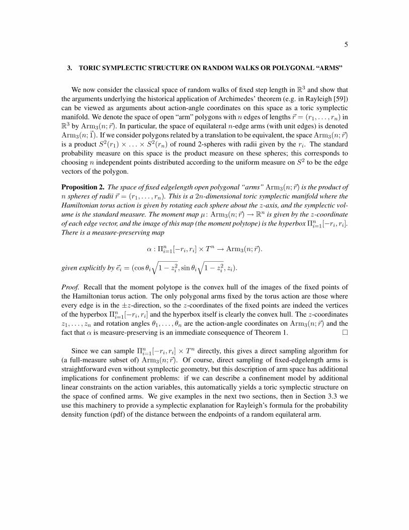
FIG. 2: This figure shows how to construct an equilateral pentagon in Pol(5;~1) using the action-angle map.First, we pick a point in the moment polytope shown in Figure 3 at center. We have now specified diagonalsd1 and d2 of the pentagon, so we may build the three triangles in the triangulation from their side lengths,as in the picture at left. We then choose dihedral angles θ1 and θ2 independently and uniformly, and jointhe triangles along the diagonals d1 and d2, as in the middle picture. The right hand picture shows the finalspace polygon, which is the boundary of this triangulated surface.

Arm3(n;~r) admits a Hamiltonian action by the Lie group SO(3) given by rotating the polygonalarm in space (this is the diagonal SO(3) action on the product of spheres) whose moment mapµ gives the vector joining the ends of the polygon. The closed polygons Pol3(n;~r) are the fiberµ−1(~0) of this map. While the group action does not generally preserve fibers of this moment map,it does preserve µ−1(~0) = Pol3(n;~r) and in this situation, we can perform what is known as asymplectic reduction (or Marsden–Weinstein–Meyer reduction [49, 50]) to produce a symplecticstructure on the quotient of the fiber µ−1(~0) by the group action. This yields a symplectic structureon the (2n − 6)-dimensional moduli space Pol3(n;~r). The symplectic measure induced by thissymplectic structure is equal to the standard measure given by pushing forward the subspace mea-sure on Pol3(n;~r) to Pol3(n;~r) because the “parent” symplectic manifold Arm3(n;~r) is a Kahlermanifold [33].

The polygon space Pol3(n;~r) is singular if

εI(~r) :=∑i∈I

ri −∑j /∈I

rj

is zero for some I ⊂ {1, . . . , n}. Geometrically, this means it is possible to construct a linearpolygon with edgelengths given by ~r. Since linear polygons are fixed by rotations around theaxis on which they lie, the action of SO(3) is not free in this case and the symplectic reductiondevelops singularities. Nonetheless, the reduction Pol3(n;~r) is a complex analytic space withisolated singularities; in particular, the complement of the singularities is a symplectic (in factKahler) manifold to which Theorem 13 applies.

Both the volume and the cohomology ring of Pol3(n;~r) are well-understood from this sym-plectic perspective [11, 32, 36, 38, 39, 46, 66]. For example:

15

Proposition 14 (Takakura [66], Khoi [38], Mandini [46]). The volume of Pol3(n;~r) is given by

Vol(Pol3(n;~r)) = − (2π)n−3

2(n− 3)!

∑I

(−1)n−|I|εI(~r)n−3,

where the sum is over all I ⊂ {1, . . . , n} such that εI(~r) > 0.

Corollary 15. The volume of the space of equilateral n-gons is

Vol(Pol3(n;~1)) = − (2π)n−3

2(n− 3)!

bn/2c∑k=0

(−1)k(n

k

)(n− 2k)n−3.

4.1. The knotting probability for equilateral hexagons

We immediately give an example application of this picture. In [16], we showed using the Fary-Milnor theorem that at least 1/3 of hexagons of total length 2 are unknotted by showing that theirtotal curvature was too small to form a knot. We could repeat the calculation using our explicitformula for the expectation of the total curvature for equilateral hexagons above, but the resultswould be disappointing; only about 27% of the space is revealed to be unknotted by this method.On the other hand action-angle coordinates, coupled with results of Calvo, immediately yield amuch better bound:

Proposition 16. At least 3/4 of the space Pol3(6;~1) of equilateral hexagons consists of unknots.

Proof. Consider the triangulation of the hexagon given by joining vertices 1, 3, and 5 by diagonalsand its corresponding action-angle coordinates α : P × T 3 → Pol3(6;~1). In [14], an impressivelydetailed analysis of hexagon space, Jorge Calvo defines a geometric2 invariant of hexagons calledthe curl which is 0 for unknots and ±1 for trefoils. In the proof of his Lemma 16, Calvo observesthat any knotted equilateral hexagon with curl +1 has all three dihedral angles between 0 and π.

The rest of the proof is elementary, but we give all the steps here as this is the first of many sucharguments below. Formally, the knot probability is the expected value of the characteristic function

χknot(p) =

{1 if p is knotted,0 if p is unknotted.

2 Interestingly, curl is independent from topological invariant given by the handedness of the trefoil, so there are actuallyfour different types of equilateral hexagonal trefoils.

16

By Calvo’s work, χknot is bounded above by the sum of characteristic functions χcurl=+1 +χcurl=−1

and χcurl=+1 is bounded above by the simpler characteristic function

χ(d1, d2, d3, θ1, θ2, θ3) =

{1 if θi ∈ [0, π] for i ∈ {1, 2, 3},0 otherwise.

Now Theorem 13 tells us that almost all of Pol3(6;~1) is a toric symplectic manifold, so (2) ofTheorem 1 holds for integrals over this polygon space. In particular, χ doesn’t depend on the di,so its expected value over Pol3(6;~1) is equal to its expected value over the torus T 3 of θi. Thisexpected value is clearly 1/8, and a similar argument holds for χcurl=−1. This means that the knotprobability is no more than 1/4, as desired.

Of course, this bound is still a substantial underestimate of the fraction of unknots. Over a12 hour run of the “PTSMCMC” Markov chain sampler of Section 5.5, we examined 1,318,001equilateral hexagons and found 173 knots. Using the 95% confidence level Geyer IPS error esti-mators of Section 5.3, we estimate the knot probability among unconfined equilateral hexagons tobe 1.3× 10−4 ± 0.2× 10−4, or between 1.1 and 1.5 in 10,000.

4.2. The Fan Triangulation and Chordlengths

While Theorem 13 applies to any triangulation, we now work out the details for a particulartriangulation. The “fan” triangulation is created by joining vertex v1 of the polygon to verticesv3, . . . , vn−1. This gives rise to the following set of triangulation inequalities. As shown in Fig-ure 3, we number the diagonals d1, . . . , dn−3 so that the first triangle has edgelengths d1, r1, r2,the last triangle has edgelengths dn−3, rn−1, rn, and all the triangles in between have edgelengthsin the form di, di+1, ri+2. The corresponding triangulation inequalities, which we call the “fantriangulation inequalities” are:

|r1 − r2| ≤ d1 ≤ r1 + r2ri+2 ≤ di + di+1

|di − di+1| ≤ ri+2|rn − rn−1| ≤ dn−3 ≤ rn + rn−1 (16)

Definition 17. The fan triangulation polytope Pn(~r) ⊂ Rn−3 is the moment polytope forPol3(n;~r) corresponding to the fan triangulation and is determined by the fan triangulation in-equalities (16). The fan triangulation polytopes P5(~1) and P6(~1) are shown in Figure 3.

This description of the moment polytope follows directly from Theorem 13.

Applying Theorem 1 to this situation gives necessary and sufficient conditions for uniformsampling on Pol3(n;~r). These could be used to test proposed polygon sampling algorithms givenstatistical tests for uniformity on convex subsets of Euclidean space and on the (n− 3)-torus.

17

v1

v2

v3

v4

v5

v6

v7

d1

d2

d3

d4

00

1

2

1 2

(2, 3, 2)

(0, 0, 0)(2, 1, 0)

Fan TriangulationFan Triangulation polytope

for Pol(5;~1)Fan Triangulation polytope

for Pol(6;~1)

FIG. 3: This figure shows the fan triangulation of a 7-gon on the left and the corresponding moment poly-topes for equilateral space pentagons and equilateral space hexagons. For the pentagon moment polytope,we show the square with corners at (0, 0) and (2, 2) to help locate the figure, while for the hexagon momentpolytope, we show the box with corners at (0, 0, 0) and (2, 3, 2) to help understand the geometry of the fig-ure. The vertices of the polytopes correspond to polygons fixed by the torus action given by rotating aroundthe diagonals. For instance, the (2, 2) point in the pentagon’s moment polytope corresponds to the config-uration given by an isoceles triangle with sides 2, 2, and 1. The diagonals lie along the long sides; rotatingaround them is a rotation of the entire configuration in space, and is hence trivial because we are consideringequivalence classes up to the action of SO(3). The (2, 3, 2) point in the hexagon’s moment polytope corre-sponds to a completely flat (or “lined”) configuration double-covering a line segment of length 3. Here allthe diagonals lie along the same line and rotation around the diagonals does nothing.

Proposition 18. A polygon in Pol3(n;~r) is sampled according to the standard measure if and onlyif its diagonal lengths d1 = |v1 − v3|, d2 = |v1 − v4|, . . . , dn−3 = |v1 − vn−1| are uniformlysampled from the fan polytope Pn(~r) and its dihedral angles around these diagonals are sampledindependently and uniformly in [0, 2π).

The fan triangulation polytope also gives us a natural way to understand the probability distri-bution of chord lengths of a closed random walk. To fix definitions,

Definition 19. Let ChordLength(k, n;~r) be the length |v1 − vk+1| of the chord skipping the firstk edges in a polygon sampled according to the standard measure on Pol3(n;~r). This is a randomvariable.

The expected values of squared chordlengths for equilateral polygons have been computed bya rearrangement technique, and turn out to be quite simple:

Proposition 20 (Cantarella, Deguchi, Shonkwiler [15] and Millett, Zirbel [73]). The second mo-ment of the random variable ChordLength(k, n;~1) is k(n−k)

n−1 .

18

It is obviously interesting to know the other moments of these random variables, but this prob-lem seems considerably harder. In particular, the techniques used in the proofs of Proposition 20don’t apply to other moments of chordlength. Here is an alternate form for the chordlength problemwhich allows us to make some explicit calculations:

Theorem 21. The expected value of the random variable ChordLength(k, n;~1) is coordinatedk−1 of the center of mass of the fan triangulation polytope Pn(~1). For n between 4 and 8, theseexpectations are given by the fractions

n\k 2 3 4 5 64 15 17/15 17/156 14/12 15/12 14/127 461/385 506/385 506/385 461/3858 1,168/960 1,307/960 1,344/960 1,307/960 1,168/960

(17)

The p-th moment of ChordLength(k, n;~1) is coordinate dk−1 of the p-th center of mass of Pn(~1).

Proof. Since the measure on Pol3(n;~1) is invariant under permutations of the edges, the pdf ofchord length for any chord skipping k edges must be the same as the pdf for the length of thechord joining v1 and vk+1. But this chord is a diagonal of the fan triangulation, so its length is thecoordinate dk−1 of the fan triangulation polytope Pn(~1). Since these chord lengths don’t dependon dihedral angles, their expectations over polygon space are equal to their expectations over Pn(~1)by (2) of Theorem 1, which applies by Theorem 13. But the expectation of a power of a coordinateover a region is simply a coordinate of the corresponding center of mass. We obtained the results inthe table by a direct computer calculation using polymake [27], which decomposes the polytopesinto simplices and computes the center of mass as a weighted sum of simplex centers of mass.

It would be very interesting to get a general formula for these polytope centers of mass.

4.3. Closed polygons in (rooted) spherical confinement

Following Diao et. al. [22], we say that a polygon p is in rooted spherical confinement of radiusR if every vertex of the polygon is contained in a sphere of radius R centered at the first vertexof the polygon. As a subspace of the space of closed polygons of fixed edgelengths, the space ofconfined closed polygons inherits a toric symplectic structure. In fact, the moment polytope forthis structure is a very simple subpolytope of the fan triangulation polytope:

Definition 22. The confined fan polytope Pn,R(~r) ⊂ Pn(~r) is determined by the fan triangulationinequalities (16) and the additional linear inequalities di ≤ R.

19

As before, we immediately have action-angle coordinates Pn,R(~r) × Tn−3 on the space ofrooted confined polygons. We note that the vertices of the confined fan triangulation polytopecorresponding to a space of confined polygons are not all fixed points of the torus action sincethis is not the entire moment polytope; new vertices have been added by imposing the additionallinear inequalities. As before, we get criteria for sampling confined polygons (directly analogousto Proposition 18 for unconfined polygons):

Proposition 23. A polygon in Pol3(n;~r) is sampled according to the standard measure on rootedsphere-confined closed space polygons in a sphere of radius R if and only if its diagonal lengthsd1 = |v1 − v3|, d2 = |v1 − v4|, . . . , dn−3 = |v1 − vn−1| are uniformly sampled from the confinedfan polytope Pn,R(~r) and its dihedral angles around these diagonals are sampled independentlyand uniformly in [0, 2π).

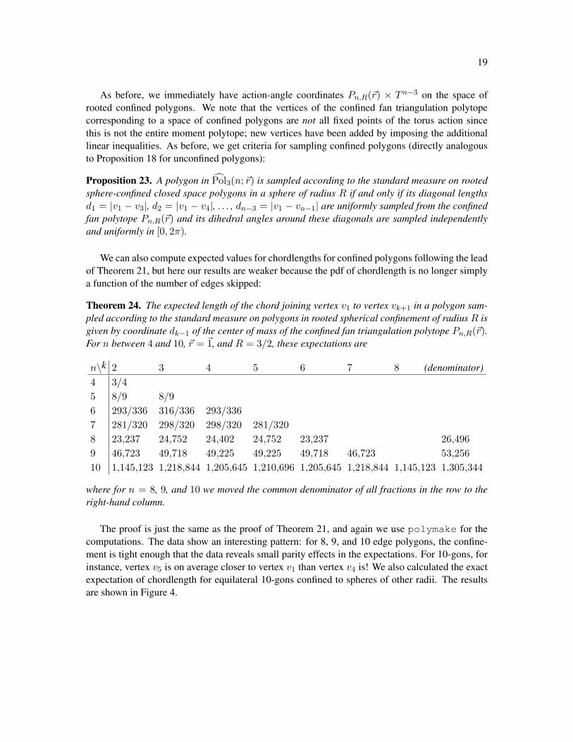
We can also compute expected values for chordlengths for confined polygons following the leadof Theorem 21, but here our results are weaker because the pdf of chordlength is no longer simplya function of the number of edges skipped:

Theorem 24. The expected length of the chord joining vertex v1 to vertex vk+1 in a polygon sam-pled according to the standard measure on polygons in rooted spherical confinement of radius R isgiven by coordinate dk−1 of the center of mass of the confined fan triangulation polytope Pn,R(~r).For n between 4 and 10, ~r = ~1, and R = 3/2, these expectations are

n\k 2 3 4 5 6 7 8 (denominator)4 3/45 8/9 8/96 293/336 316/336 293/3367 281/320 298/320 298/320 281/3208 23,237 24,752 24,402 24,752 23,237 26,4969 46,723 49,718 49,225 49,225 49,718 46,723 53,25610 1,145,123 1,218,844 1,205,645 1,210,696 1,205,645 1,218,844 1,145,123 1,305,344

where for n = 8, 9, and 10 we moved the common denominator of all fractions in the row to theright-hand column.

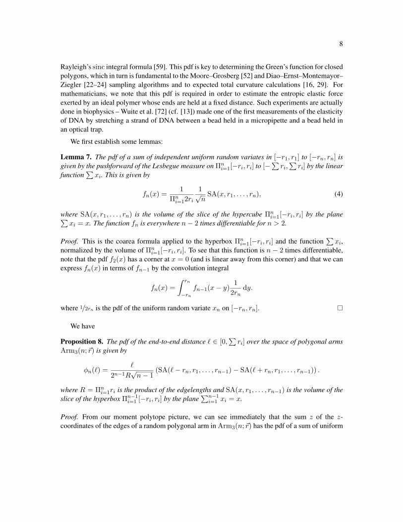
The proof is just the same as the proof of Theorem 21, and again we use polymake for thecomputations. The data show an interesting pattern: for 8, 9, and 10 edge polygons, the confine-ment is tight enough that the data reveals small parity effects in the expectations. For 10-gons, forinstance, vertex v5 is on average closer to vertex v1 than vertex v4 is! We also calculated the exactexpectation of chordlength for equilateral 10-gons confined to spheres of other radii. The resultsare shown in Figure 4.

20

2 4 6 8 10k

0.5

1.0

1.5

Expected Chord Length

FIG. 4: Each line in this graph shows the expected length of the chord joining vertices v1 and vk in a randomequilateral 10-gon. The 10-gons are sampled from the standard measure on polygons in rooted sphericalconfinement. From bottom to top, the confinement radii are 1.25, 1.5, 1.75, 2, 2.5, 3, 4, and 5. Polygonsconfined in a sphere of radius 5 are unconfined. Note the small parity effects which emerge in tighterconfinement. These are exact expectations, not the result of sampling experiments.

5. MARKOV CHAIN MONTE CARLO FOR CLOSED AND CONFINED RANDOM WALKS

We have now constructed the action-angle coordinates on several spaces of random walks,including closed walks, closed walks in rooted spherical confinement, standard (open) randomwalks, and open random walks confined to half-spaces or slabs. In each case, the action-anglecoordinates have allowed us to prove some theorems and make some interesting exact computationsof probabilities on the spaces. To address more complicated (and physically interesting) questions,we will now turn to numerically sampling these spaces.

Numerical sampling of closed polygons underlies a substantial body of work on the geometryand topology of polymers and biopolymers (see the surveys of [55] and [6], which contain morethan 200 references), which is a topic of interest in statistical physics. Many of the physics ques-tions at issue in these investigations seem to be best addressed by computation. For instance, whileour methods above gave us simple (though not very tight) theoretical bounds on the fraction of un-knots among equilateral 6-gons, a useful theoretical bound on, say, the fraction of unknots among1,273-gons seems entirely out of reach. On the other hand, it is entirely reasonable to work on de-veloping well-founded algorithms with verified convergence and statistically defensible error barsfor experimental work on such questions, and that is precisely our aim in this part of the paper.

5.1. Current Sampling Algorithms for Random Polygons

A wide variety of sampling algorithms for random polygons have been proposed. They fallinto two main categories: Markov chain algorithms such as polygonal folds [51] or crankshaft

21

moves [40, 70] (cf. [1] for a discussion of these methods) and direct sampling methods such asthe “triangle method” [53] or the “generalized hedgehog” method [69] and the methods of Mooreand Grosberg [52] and Diao, Ernst, Montemayor, and Ziegler [22–24] which are both based on the“sinc integral formula” (7).

Each of these approaches has some defects. No existing Markov chain method has been provedto converge to the standard measure, though it is generally conjectured that they do. It is un-clear what measure the generalized hedgehog method samples, while the triangle method clearlysamples a submanifold3 of polygon space. The Moore–Grosberg algorithm is known to samplethe correct distribution, but faces certain practical problems. It is based on computing succes-sive piecewise-polynomial distributions for diagonal lengths of a closed polygon and directly sam-pling from these one-dimensional distributions. There is no problem with the convergence of thismethod, but the difficulty is that the polynomials are high degree with large coefficients and manyalmost-cancellations, leading to significant numerical problems with accurately evaluating them4.These problems are somewhat mitigated by the use of rational and multiple-precision arithmeticin [52], but the number of edges in polygons sampled with these methods is inherently limited.For instance, the text file giving the coefficients of the polynomials needed to sample a randomclosed 95-gon is over 25 megabytes in length. Diao et. al. avoid this problem by approximatingthese distributions by normals, but this approximation means that they are not quite5 sampling thestandard measure on polygon space.

5.2. The Toric Symplectic Markov Chain Monte Carlo Algorithm

We introduce a Markov Chain Monte Carlo algorithm for sampling toric symplectic mani-folds with an adjustable parameter β ∈ (0, 1) explained below. We will call this the TORIC-SYMPLECTIC-MCMC(β) algorithm or TSMCMC(β) for convenience. Though we intend to ap-ply this algorithm to our random walk spaces, it works on any toric symplectic manifold, so we statethe results in this section and the next for an arbitrary toric symplectic manifold M2n with momentmap µ :M → Rn, moment polytope P , and action-angle parametrization α :P × Tn → M . Themethod is based on a classical Markov chain for sampling convex regions of Rn called the “hit-and-run” algorithm: choose a direction at random and sample along the intersection of that ray withthe region to find the next point in the chain. This method was introduced by Boneh and Golan [9]

3 It is hard to know whether this restriction is important in practice. The submanifold may be sufficiently “well-distributed” that most integrands of interest converge anyway. Or perhaps calculations performed with the trianglemethod are dramatically wrong for some integrands!

4 Hughes discusses these methods in Section 2.5.4 of his book on random walks [35], attributing the formula rederivedby Moore and Grosberg [52] to a 1946 paper of Treloar [68]. The problems with evaluating these polynomialsaccurately were known by the 1970’s, when Barakat [5] derived an alternate expression for this probability densitybased on Fourier transform methods.

5 Again, it is unclear what difference this makes in practice.

22

and independently by Smith [62] as a means of generating random points in a high-dimensionalpolytope. There is a well-developed theory around this method which we will be able to make useof below.

The parameter β controls the relative weight given to the action and angle variables. At eachstep of TSMCMC(β), with probability β we update the action variables by sampling the momentpolytope P using hit-and-run and with probability 1−β we update the angle variables by samplingthe torus Tn uniformly. When β = 1/2 this is analogous to the random scan Metropolis-within-Gibbs samplers discussed by Roberts and Rosenthal [60] (see also [41]). The adjustable parameterβ allows us to tune the speed and accuracy of Monte Carlo integration using TSMCMC(β). Asa trivial example, if we use TSMCMC(β) to numerically integrate a functional which is almostconstant in the angle variables, then we should let β be very close to 1.

TORIC-SYMPLECTIC-MCMC(~p, ~θ, β)prob = UNIFORM-RANDOM-VARIATE(0, 1)if prob < β

then � Generate a new point in P using the hit-and-run algorithm.~v = RANDOM-DIRECTION(n)(t0, t1) = FIND-INTERSECTION-ENDPOINTS(P, ~p,~v)t = UNIFORM-RANDOM-VARIATE(t0, t1)~p = ~p+ t~v

else � Generate a new point in Tn uniformly.for ind = 1 to n

do θind = UNIFORM-RANDOM-VARIATE(0, 2π)return (~p,~θ)

We now prove that the distribution of samples produced by this Markov chain converges geo-metrically to the distribution generated by the symplectic volume on M2n. First, we show that thesymplectic measure on M is invariant for TSMCMC.

To do so, recall that for any Markov chain Φ on a state space X , we can define the m-steptransition probability Pm(x,A) to be the probability that an m-step run of the chain starting at xlands in the set A. This defines a measure Pm(x, ·) on X . The transition kernel P = P1 is calledreversible with respect to a probability distribution π if∫

Aπ(dx)P(x,B) =

∫Bπ(dx)P(x,A) for all measurable A,B ⊂ X. (18)

In other words, the probability of moving from A to B is the same as the probability of movingfrom B to A. If P is reversible with respect to π, then π is invariant for P: letting A = X in (18),we see that πP = π.

23

In TSMCMC(β), the transition kernel P = βP1 + (1 − β)P2, where P1 is the hit-and-runkernel on the moment polytope and P2(~θ, ·) = τ , where τ is the uniform measure on Tn. Sincehit-and-run is reversible on the moment polytope [63] and since P2 is obviously reversible withrespect to τ , we have:

Proposition 25. TSMCMC(β) is reversible with respect to the symplectic measure ν induced bysymplectic volume on M . In particular, ν is invariant for TSMCMC(β).

Recall that the total variation distance between two measures η1, η2 on a state space X is givenby

|η1 − η2|TV := supA any measurable set

|η1(A)− η2(A)|.

We can now prove geometric convergence of the sample measure generated by TSMCMC(β) tothe symplectic measure in total variation distance.

Theorem 26. Suppose that M2n is a toric symplectic manifold with moment polytope P andaction-angle coordinates α : P × Tn → M2n. Further, let Pm(~p, ~θ, ·) be the m-step transitionprobability of the Markov chain given by TORIC-SYMPLECTIC-MCMC(β) and let ν be the sym-plectic measure on M2n.

There are constants R <∞ and ρ < 1 so that for any (~p, ~θ) ∈ int(P )× Tn,∣∣∣α?Pm(~p, ~θ, ·)− ν∣∣∣TV

< Rρm.

That is, for any choice of starting point, the pushforward by α of the probability measure generatedby TORIC-SYMPLECTIC-MCMC(β) on P × Tn converges geometrically (in the number of stepstaken in the chain) to the symplectic measure on M2n.

Proof. Let λ be Lebesgue measure on the moment polytope P and, as above, let τ be uniformmeasure on the torus Tn. By Theorem 1, it suffices to show that∣∣∣Pm(~p, ~θ, ·)− λ× τ

∣∣∣TV

< Rρm.

Since the transition kernels P1 and P2 commute, for any non-negative integers a and b and parti-tions i1, . . . , ik of a and j1, . . . , j` of b we have(P i11 P

j12 · · · P

ik1 P

j`2

)(~p, ~θ, ·) =

(Pa1Pb2

)(~p, ~θ, ·) = Pa1 (~p, ·)× Pb2(~θ, ·) = Pa1 (~p, ·)× τ, (19)

where the last equality follows from the fact that P2(~θ, ·) = τ for any ~θ ∈ Tn.

24

The total variation distance between product measures is bounded above by the sum of the totalvariation distances of the factors (this goes back at least to Blum and Pathak [8]; see Sendler [61]for a proof), so we have that∣∣∣Pa1 (~p, ·)× Pb2(~θ, ·)− λ× τ

∣∣∣TV

= |Pa1 (~p, ·)× τ − λ× τ |TV

≤ |Pa1 (~p, ·)− λ|TV + |τ − τ |TV (20)

= |Pa1 (~p, ·)− λ|TV .

Using a result of Smith [63, Theorem 3], the right hand side is bounded above by(

1− ξn2n−1

)a−1

where ξ is the ratio of the volume of P and the volume of the smallest round ball containing P . Let

κ :=(

1− ξ

n2n−1

).

Then combining (19), (20), and the binomial theorem yields∣∣∣Pm(~p, ~θ, ·)− λ× τ∣∣∣TV

=∣∣∣(βP1 + (1− β)P2)m (~p, ~θ, ·)− λ× τ

∣∣∣TV

=

∣∣∣∣∣m∑i=0

(m

i

)βm−i(1− β)i

(Pm−i1 (~p, ·)× τ − λ× τ

)∣∣∣∣∣TV

≤m∑i=0

(m

i

)βm−i(1− β)iκm−i−1

=1κ

(1 + β(κ− 1))m =1κ

(1− βξ

n2n−1

)m.

The ratio ξ of the volume of P and the volume of smallest round ball containing P is always apositive number with absolute value less than 1, so 0 < 1 − βξ/n2n−1 < 1. This completes theproof.

This proposition provides a comforting theoretical guarantee that TORIC-SYMPLECTIC-MCMC(β) will eventually work. The proof provides a way to estimate the constants R and ρ.However, in practice, these upper bounds are far too large to be useful. Further, the rate of conver-gence for any given run will depend on the shape and dimension of the moment polytope P and onthe starting position x. There is quite a bit known about the performance of hit-and-run in generaltheoretical terms; we recommend the excellent survey article of Andersen and Diaconis [2]. Togive one example, Lovasz and Vempala have shown [44] (see also [43]) that the number of steps ofhit-and-run required to reduce the total variation distance between Pm(x, ·) and Lebesgue measureby an order of magnitude is proportional6 to n3 where n is the dimension of the polytope.

6 The constant of proportionality is large and depends on the geometry of the polytope, and the amount of time requiredto reduce the total variation distance to a fixed amount from the start depends on the distance from the starting pointto the boundary of the polytope.

25

5.3. The Markov Chain CLT and Geyer’s IPS Error Bounds for TSMCMC integration

We now know that the TSMCMC(β) algorithm will eventually sample from the correct prob-ability measure on any toric symplectic manifold, and in particular from the correct probabilitydistributions on closed and confined random walks. We should pause to appreciate the significanceof this result for a moment – while many Markov chain samplers have been proposed for closedpolygons, none have been proved to converge to the correct measure. Further, there has never beena Markov chain sampler for closed polygons in rooted spherical confinement (or, as far as we know,for slab-confined or half-space confined arms).

However, the situation remains in some ways unsatisfactory. If we wish to compute the prob-ability of an event in one of these probability spaces of polygons, we must do an integral overthe space by collecting sample values from a Markov chain. But since we do not have any ex-plicit bounds on the rate of convergence of our Markov chains, we do not know how long to runthe sampler, or how far the resulting sample mean might be from the integral over the space. Toanswer these questions, we need two standard tools: the Markov Chain Central Limit Theoremand Geyer’s Initial Positive Sequence (IPS) error estimators for MCMC integration [28]. For theconvenience of readers unfamiliar with these methods, we summarize the construction here. Sincethis is basically standard material, many readers may wish to skip ahead to the next section.

Combining Proposition 26 with [67, Theorem 5] (which is based on [20, Corollary 4.2]) yieldsa central limit theorem for the TORIC-SYMPLECTIC-MCMC(β) algorithm. To set notation, a runof the TSMCMC(β) algorithm produces the sequence of points ((~p0, ~θ0), (~p1, ~θ1), . . .), where theinitial point (~p0, ~θ0) is drawn from some initial distribution (for example, a delta distribution). Forany run R, let

SMean(f ;R,m) :=1m

m∑k=1

f(~pk, ~θk)

be the sample mean of the values of a function f :M2n → R over the first m steps in R. Wewill use “f” interchangeably to refer to the original function f :M2n → R or its expression inaction-angle coordinates f ◦ α :P × Tn → R.

Let E(f ; ν) be the expected value of f with respect to the symplectic measure ν on M . Thenfor each positive integer m the normalized sample error

√m(SMean(f ;R,m)− E(f ; ν))

is a random variable (as it depends on the various random choices in the run R).

Proposition 27. Suppose f is a square-integrable real-valued function on the toric symplecticmanifold M2n. Then regardless of the initial distribution, there exists a real number σ(f) so that

√m(SMean(f ;R,m)− E(f ; ν)) w−→ N (0, σ(f)2), (21)

where N (0, σ(f)2) is the Gaussian distribution with mean 0 and standard deviation σ(f) and thesuperscript w denotes weak convergence.

26

Given σ(f) and a run R, the range SMean(f ;R,m) ± 1.96σ(f)/√m is an approximate 95%

confidence interval for the true expected value E(f ; ν). Abstractly, we can find σ(f) as follows.

The variance of the left hand side of (21) is

mVar(SMean(f ;R,m)) =1m

m∑i=1

Var(f(~pi, ~θi)) +1m

m∑i=1

m∑j=1

Cov(f(~pi, ~θi), f(~pj , ~θj)).

Since the convergence in Proposition 27 is independent of the initial distribution, σ(f) will be thelimit of this quantity for any initial distribution. Following Chan and Geyer [18], suppose the initialdistribution is the stationary distribution. In that case, the quantities

γ0(f) := Var(f(~pi, ~θi))

and

γk(f) := Cov(f(~pi, ~θi), f(~pi+k, ~θi+k))

(the stationary variance and lag k autocovariance, respectively) are independent of i. Then

σ(f)2 = limm→∞

(γ0(f) + 2

m−1∑k=1

m− km

γk(f)

)= γ0(f) + 2

∞∑k=1

γk(f)

provided the sum on the right hand side converges.

In what follows it will be convenient to write the above as

σ(f)2 = γ0(f) + 2γ1(f) + 2∞∑k=1

Γk(f), (22)

where Γk(f) := γ2k(f) + γ2k+1(f). Again, we emphasize that the quantities γ0(f), γk(f),Γk(f)are associated to the stationary Markov chain.

In practice, of course, these quantities and hence this expression for σ(f) are not computable.After all, if we could sample directly from the symplectic measure on M2n there would be no needfor TSMCMC. However, as pointed out by Geyer [28], σ(f) can be estimated from the sample datathat produced SMean(f ;R,m). Specifically, we will estimate the stationary lagged autocovarianceγk(f) by the following quantity:

γk(f) =1m

m−k∑i=1

[f(~pi, ~θi)− SMean(f ;R,m)][f(~pi+k, ~θi+k)− SMean(f ;R,m)] (23)

Note that multiplication by 1/m rather than 1/m−k is not a typographical error (cf. [28], Sec 3.1).Let Γk(f) = γ2k(f) + γ2k+1(f). Then for any N > 0

σm,N (f)2 := γ0(f) + 2γ1(f) + 2N∑k=1

Γk(f) (24)

27

is an estimator for σ(f)2. We expect the Γk to decrease to zero as k →∞ since very distant pointsin the run of the Markov chain should become statistically uncorrelated. Indeed, since TSMCMCis reversible, Geyer shows this is true for the stationary chain:

Theorem 28 (Geyer [28], Theorem 3.1). Γk is strictly positive, strictly decreasing, and strictlyconvex as a function of k.

We expect, then, that any non-positivity, non-monotonicity, or non-convexity of the Γk shouldbe due to k being sufficiently large that Γk is dominated by noise. In particular, this suggests that areasonable choice for N in (24) is the first N such that ΓN ≤ 0, since the terms past this point willbe dominated by noise and hence tend to cancel each other.

Definition 29. Given a function f and a length-m run of the TSMCMC algorithm as above, let Nbe the largest integer so that Γ1(f), . . . , ΓN (f) are all strictly positive. Then the initial positivesequence estimator for σ(f) is

σm(f) := σm,N (f) = γ0(f) + 2γ1(f) + 2N∑k=1

Γk(f).

Slightly more refined initial sequence estimators which take into account the monotonicity andconvexity from Proposition 28 are also possible; see [28] for details.

The pleasant result of all this is that σm is a statistically consistent overestimate of the actualvariance.

Theorem 30 (Geyer [28], Theorem 3.2). For almost all sample paths of TSMCMC,

lim infm→∞

σm(f)2 ≥ σ(f)2.

Therefore, we propose the following procedure for Toric Symplectic Markov Chain Monte Carlointegration which yields statistically consistent error bars on the estimate of the true value of theintegral:

Toric Symplectic Markov Chain Monte Carlo Integration. Let f be a square-integrable func-tion on a toric symplectic manifold M2n with moment map µ : M → Rn.

1. Find the fixed points of the Hamiltonian torus action. The moment polytope P is the convexhull of the images of these fixed points under µ.

2. Convert this vertex description of P to a halfspace description. In other words, realize P asthe subset of points in Rn satisfying a collection of linear inequalities.7

7 For small problems, this can be done algorithmically [4, 19, 27]. Generally, this will require an analysis of the momentpolytope, such as the one performed above for the moment polytopes of polygon spaces.

28

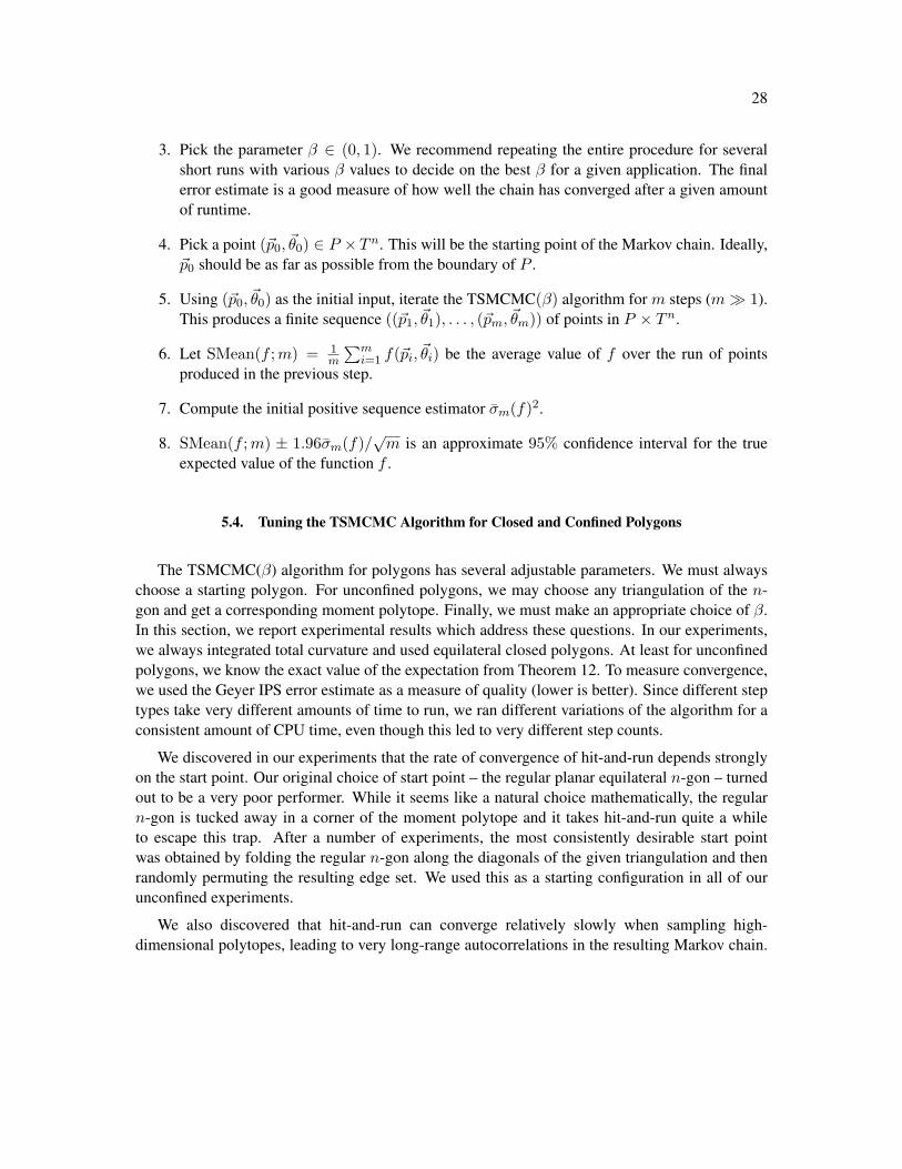
3. Pick the parameter β ∈ (0, 1). We recommend repeating the entire procedure for severalshort runs with various β values to decide on the best β for a given application. The finalerror estimate is a good measure of how well the chain has converged after a given amountof runtime.

4. Pick a point (~p0, ~θ0) ∈ P ×Tn. This will be the starting point of the Markov chain. Ideally,~p0 should be as far as possible from the boundary of P .

5. Using (~p0, ~θ0) as the initial input, iterate the TSMCMC(β) algorithm for m steps (m� 1).This produces a finite sequence ((~p1, ~θ1), . . . , (~pm, ~θm)) of points in P × Tn.

6. Let SMean(f ;m) = 1m

∑mi=1 f(~pi, ~θi) be the average value of f over the run of points

produced in the previous step.

7. Compute the initial positive sequence estimator σm(f)2.

8. SMean(f ;m) ± 1.96σm(f)/√m is an approximate 95% confidence interval for the true

expected value of the function f .

5.4. Tuning the TSMCMC Algorithm for Closed and Confined Polygons

The TSMCMC(β) algorithm for polygons has several adjustable parameters. We must alwayschoose a starting polygon. For unconfined polygons, we may choose any triangulation of the n-gon and get a corresponding moment polytope. Finally, we must make an appropriate choice of β.In this section, we report experimental results which address these questions. In our experiments,we always integrated total curvature and used equilateral closed polygons. At least for unconfinedpolygons, we know the exact value of the expectation from Theorem 12. To measure convergence,we used the Geyer IPS error estimate as a measure of quality (lower is better). Since different steptypes take very different amounts of time to run, we ran different variations of the algorithm for aconsistent amount of CPU time, even though this led to very different step counts.

We discovered in our experiments that the rate of convergence of hit-and-run depends stronglyon the start point. Our original choice of start point – the regular planar equilateral n-gon – turnedout to be a very poor performer. While it seems like a natural choice mathematically, the regularn-gon is tucked away in a corner of the moment polytope and it takes hit-and-run quite a whileto escape this trap. After a number of experiments, the most consistently desirable start pointwas obtained by folding the regular n-gon along the diagonals of the given triangulation and thenrandomly permuting the resulting edge set. We used this as a starting configuration in all of ourunconfined experiments.

We also discovered that hit-and-run can converge relatively slowly when sampling high-dimensional polytopes, leading to very long-range autocorrelations in the resulting Markov chain.

29

Following a suggestion of Soteros [64], after considerable experimentation we settled on the con-vention that a single “moment polytope” step in our implementation of TSMCMC(β) would rep-resent ten iterations of hit-and-run on the moment polytope. This reduced autocorrelations greatlyand led to better convergence overall. We used this convention for all our numerical experimentsbelow.

The TORIC-SYMPLECTIC-MCMC(β) algorithm depends on a choice of triangulation T for then-gon to determine the moment polytope P . There is considerable freedom in this choice, sincethe number of triangulations of an n-gon is the Catalan number Cn−2 ∼ 4n−2/(n − 2)3/2

√π.

We have proved above that the TORIC-SYMPLECTIC-MCMC(β) algorithm will converge for anyof these triangulations, but the rate of convergence is expected to depend on the triangulation,which determines the geometry of the moment polytope. This geometry directly affects the rate ofconvergence of hit-and-run; “long and skinny” polytopes are harder to sample than “round” ones(see Lovasz [43]).

To get a sense of the effect of the triangulation on the performance of TSMCMC(β) we setβ = 0.5 and n = 23 and ran the algorithm from 20 start points for 20,000 steps. We then took theaverage IPS error bar for expected total curvature over these 20 runs as a measure of convergence.We repeated this analysis for 300 random triangulations and 300 repeats of three triangulations thatwe called the “fan”, “teeth” and “spiral” triangulations. The results are shown in Figure 5. The def-inition of the fan and teeth triangulations will be obvious from that figure; the spiral triangulation isgenerated by traversing the n-gon in order repeatedly, joining every other vertex along the traversaluntil the triangulation is complete. Our experiments showed that this spiral triangulation was thebest performing triangulation among our candidates, so we standardized on that triangulation forfurther numerical experiments.

We then considered the effect of varying the parameter β for the TSMCMC(β) algorithm usingthe spiral triangulation. We ran a series of trials computing expected total curvature for 64-gonsover 10 minute runs, while varying β from 0.05 (almost all dihedral steps) to 0.95 (almost allmoment polytope steps) over 10 minute runs. We repeated each run 50 times to get a sense of thevariability in the Geyer IPS error estimators for different runs. Since dihedral steps are considerablyfaster than moment polytope steps, the step counts varied from about 1 to 9 million. The resultingGeyer IPS error estimators are shown in Figure 6. Our recommendation from these experiments isto use the spiral triangulation and β = 0.5 for experiments with unconfined polygons. From the50 runs using the recommended β = 0.5, the run with the median IPS error estimate producedan expected total curvature estimate of 101.724 ± 0.142 using about 4.6 million samples; recallthat we computed in Table II that the expected value of total curvature for equilateral, unconfined64-gons is a complicated fraction close to 101.7278.

30

[0.117, 0.127] 0.123 [0.153, 0.181] [0.158, 0.184]spiral random fan teeth

FIG. 5: We tested the average IPS 95% confidence error estimate for the expected value of total curvatureover random equilateral 23-gons over 20 runs of the TSMCMC(0.5) algorithm. Each run had a startingpoint generated by folding and permuting a regular n-gon as described above, and ran for 20,000 steps.We tried 300 random n-gons and 300 repetitions of the same procedure for the “spiral”, “fan”, and “teeth”triangulations shown above. Below each triangulation is shown the range of average error bars observed over300 repetitions of the 20-start-point trials; for the random triangulation we report the best average error barover a single 20-start-point-trial observed for any of the 300 random triangulations we computed. We cansee that the algorithm based on the spiral triangulation generally outperforms algorithms based on even thebest of the 300 random triangulations, while algorithms based on the fan and teeth triangulations convergedmore slowly.

0.05 0.25 0.5 0.75 0.95Β

1.2 ´ 10-1

7.5 ´ 10-1

1.4

IPS error

FIG. 6: The figure above shows a box-and-whisker plot for the IPS error estimators observed in computingexpected total curvature over 50 runs of the TSMCMC(β) algorithm for various values of β. The boxesshow the 1/4 to 3/4 quantiles of the data, while the whiskers extend from the 0.05 quantile to the 0.95quantile. While the whiskers show that there is plenty of variability in the data, the general trend is that theperformance of the algorithm improves rapidly as β varies from 0.05 to 0.25, modestly as β varies from 0.25to 0.5 and is basically constant for β from 0.5 to 0.95.

5.5. Crankshafts, folds and permutation steps for unconfined equilateral polygons

If we are dealing with unconfined equilateral polygons, we can define a transformationfrom Pol3(n;~1) to itself by permuting the edge set of the polygon. Since the symplec-tic measure on the space Pol3(n;~1) = Pol3(n;~1)/ SO(3) of unconfined equilateral poly-

31

gons agrees with the standard measure, which is the pushforward of the subspace measure onPol3(n;~1) ⊂ Arm3(n;~1) = S2(1)× . . .× S2(1), the action of the symmetric group Sn whichpermutes edges is measure-preserving on Pol3(n;~1). As a consequence, we will see that we canmix permutation steps with standard TSMCMC steps without losing geometric convergence or theapplicability of the Central Limit Theorem. Such a Markov chain is a mixture of dihedral anglesteps, moment polytope steps, and permutation steps in some proportion. It is interesting to notethat we can recover algorithms very similar to the standard “crankshaft” and “fold” Markov chainsby allowing no moment polytope steps in the chain.

Since previous authors have observed that adding permutation steps can significantly speed upconvergence in polygon samplers [1], we now experiment to see whether our algorithm, too, canbe improved by mixing in some permutations. More precisely, we can define a new Markov chainPOLYGON-PERMUTATION on Pol3(n;~1) by permuting edges at each step:

POLYGON-PERMUTATION(pol)

σ = UNIFORM-PERMUTATION(n)pol = PERMUTE-EDGES(pol, σ)return pol

Since the symplectic measure on Pol3(n;~1) is permutation-invariant, the symplectic measure isstationary for POLYGON-PERMUTATION.

Now, we can mix TSMCMC(β) with POLYGON-PERMUTATION to get the followingPERMUTATION-TORIC-SYMPLECTIC-MCMC(β, δ) algorithm, where δ ∈ [0, 1) gives theprobability of doing a permutation step rather than a TSMCMC(β) step. Recall thatα :P × Tn−3 → Pol3(n;~1) is the action-angle parametrization, where P is the moment polytopeinduced by the chosen triangulation.

PERMUTATION-TORIC-SYMPLECTIC-MCMC(~p, ~θ, β, δ)prob = UNIFORM-RANDOM-VARIATE(0, 1)if prob < δ

then (~p, ~θ ) = α−1(POLYGON-PERMUTATION(α(~p, ~θ )))else (~p, ~θ ) = TORIC-SYMPLECTIC-MCMC(~p, ~θ, β)

return (~p, ~θ )

Although POLYGON-PERMUTATION is not ergodic, the fact that it is stationary with respect tothe symplectic measure is, by combining Proposition 26 and [67, Proposition 3], enough to implythat PERMUTATION-TORIC-SYMPLECTIC-MCMC(β, δ) is (strongly) uniformly ergodic.

32

Proposition 31. Let P be the transition kernel for PTSMCMC(β, δ) with 0 < β < 1 and δ < 1and let ν be the symplectic measure on Pol3(n;~1). Then there exist constants R < ∞ and ρ < 1so that for any (~p, ~θ ) ∈ int(P )× Tn−3,∣∣∣α?Pm(~p, ~θ, ·)− ν

∣∣∣TV

< Rρm.

Just as in Proposition 27, since PTSMCMC(β, δ) is uniformly ergodic and reversible with re-spect to symplectic measure, it satisfies a central limit theorem:

Proposition 32. Suppose f : Pol3(n;~1) → R is square-integrable. For any run R ofPTSMCMC(β, δ), let SMean(f ;R,m) be the sample mean of the value of f over the first m stepsof R. Then there exists a real number σ(f) so that

√m(SMean(f ;R,m)− E(f ; ν)) w−→ N (0, σ(f)2).

The rest of the machinery of Section 5.3, including the initial positive sequence estimator forσ(f)2, also applies. As a consequence, we get a modified Toric Symplectic Markov Chain MonteCarlo Integration procedure adapted to unconfined, equilateral polygons. Note that the full sym-metric group Sn does not act on Pol3(n;~r) when not all ri are equal, so PTSMCMC(β, δ) cannotbe used to sample non-equilateral polygons. However when many edgelengths are equal, a sub-group of the symmetric group which permutes only those edges certainly acts on Pol3(n;~r). Werecommend making use of this smaller set of permutations when possible. Permuting edges neverpreserves spherical confinement, so PTSMCMC(β, δ) is inapplicable to confined polygon sam-pling.

Having defined PTSMCMC(β, δ) and settled on a canonical starting point (the folded, permutedregular n-gon) and triangulation (the spiral), it remains to decide on the best values of β and δ. Thequestion is complicated by the fact that the three different types of steps – permutations, foldingsteps, and moment-polytope hit-and-run steps – take different amounts of CPU time. To attempt toevaluate the various possibilities fairly, we ran experiments computing the expected total curvaturefor 64-gons where each experiment ran for 10 minutes of CPU time, completing between 2 millionand 15 million steps depending on the mixture of step types. We measured the 95% confidenceIPS error bars for each run, producing the data in Figure 7, and used the size of this error bar as ameasure of convergence.

The data in Figure 7 show that the fraction δ of permutation steps is the most important factorin determining the rate of convergence in the PTSMCMC(β,δ) algorithm. This shows that theextra complication in defining PTSMCMC(β,δ) for unconfined equilateral polygons is worth it:the error bars produced by PTSMCMC(β,δ) to compute the expected total curvature of unconfinedequilateral 64-gons are anywhere from 3 to 30 times smaller than the error bars for TSMCMC(β).

Larger values of β produce smaller error bars when δ = 0, meaning that a large fraction ofmoment polytope steps are needed to produce mixing when there are no permutation steps. On the

33

0.30.7

0.3

0.70.1

0.2

0.3

β

δ

IPS error

0.30.7

0.3

0.7

0.01

0.02

0.03

β

δ

IPS error

FIG. 7: This plot shows the IPS error estimator for the average total curvature of unconfined equilateral64-gons. The IPS error was computed for 10 minute runs of the PTSMCMC(β,δ) Markov chain algorithm.The values of δ (the fraction of permutations among all steps) ranged from 0 to 0.95 in steps of 0.05, whilethe values of β (the fraction of moment polytope steps among non-permutation steps) ranged from 0 to 0.95in steps of 0.05. When δ = 0, this is just the TSMCMC(β) chain; removing those runs yields the plot on theright. We observed that convergence was very sensitive to δ, with error bars improving dramatically as soonas the fraction of permutation steps becomes positive: even the worst PTSMCMC(β,δ) run with δ > 0 haderror bars 3 times smaller than the error bars of the best TSMCMC(β) run. From the view at right, we cansee that the error bars continue to improve more modestly as δ increases. Varying β has little effect on theerror estimate when δ is large.

other hand, as we can see in Figure 8, even when δ = 0.05 the permutation steps provide enoughmixing that β has virtually no effect on the IPS standard deviation estimator. In this case, theeffect of β on the size of the error bars is due to the fact that dihedral steps are faster than momentpolytope steps, so runs with small β produce more samples and hence smaller error bars.

ææ

æ

ææ

æ

æ æ

æ

ææ æ

æ æ

æ

æ

æ

æ

æ

0 0.5 1

0.01

0.02

0.03

β

IPS error

æ æ æ æ æ æ æ æ æ æ æ ææ æ æ

ææ

ææ

0 0.5 1

10

20

30

β

IPS standard deviation

FIG. 8: These plots show the IPS error estimator and the IPS standard deviation estimator for the averagetotal curvature of unconfined equilateral 64-gons using 10-minute runs of PTSMCMC(β, 0.05). Althoughthe IPS error estimate decreases as β decreases, the plot on the right demonstrates that the IPS standarddeviation estimator is essentially constant – and presumably close to the true standard deviation of thetotal curvature function – across the different values of β. Since the IPS error estimate is proportional tothe standard deviation estimate divided by the square root of the number of samples, we can see that thevariation in IPS error bars for these runs is almost entirely due to the difference in the number of samples.

Once δ is large, varying β seems to have little effect on the convergence rate. In fact, though

34

our theory above no longer proves convergence, we seem to get a very competitive algorithmby removing moment polytope steps altogether (β = 0) and performing only permutations anddihedral steps. This algorithm corresponds to the “fold or crankshaft with permutations mixed in”method.

In practice, we make a preliminary recommendation of δ = 0.9 and β = 0.5 for experimentalwork. These parameters guarantee convergence (by our work above) while optimizing the con-vergence rate. Using these recommended parameters, a 10 minute run of PTSMCMC(0.5,0.9) forunconfined, equilateral 64-gons produced just under 7 million samples and an expected total cur-vature of 101.7276±0.0044, which compares quite favorably to the actual expected total curvatureof 101.7278.

Taking out the β = 0 runs, we observed that the absolute error in our computations of expectedtotal curvature was less than our error estimate in 361 of 380 runs (95%), which is exactly whatwe would expect from a 95% confidence value estimator. We take this as solid evidence that theMarkov chain is converging and the error estimators are working as expected.

5.6. Calculations on confined polygons

Recall from Definition 22 that a polygon is in spherical confinement in a sphere of radius Rcentered at vertex v1 of the polygon if the vector ~d of fan diagonals of the polygon lies in the con-fined fan polytope Pn,R(~r). This means that we can sample such polygons uniformly by restrictingthe hit-and-run steps in TSMCMC(β) to the confined fan polytope Pn,R(~r).

We again only explored the situation for equilateral polygons of edge length one. After someexperimentation, we settled on the “folded triangle” as a start point. This polygon is constructed bysetting each diagonal length di to one and choosing dihedrals randomly. This polygon is containedin spherical confinement for every R ≥ 1, so we could use it for all of our experiments. Weinvestigated 23-gons confined to spheres of radius 2, 4, 6, 8, 10 and 12, measuring the Geyer IPSerror estimate for values of β selected from 0.05 (almost all dihedral steps) to 0.95 (almost allmoment polytope steps) over 10 minute runs. Again, since dihedral steps are faster to run thanmoment polytope steps, the step counts varied over the course of the experiments. For instance, inthe radius 2 experiments, we observed step counts as high as 35 million and as low as 7 millionover runs with various β values. Our integrand was again total curvature. Since we do not havean exact solution for the expected total curvature of a confined n-gon, we were unable to checkwhether the error bars predicted actual errors. However, it was comforting to note that the answerswe got from runs with various parameters were very consistent. We ran each experiment 50 timesto get a sense of the repeatability of the Geyer IPS error bar; the results are shown in Figure 9.

We observed first that there is a clear trend in the error bar data. For the tightly confinedruns, there was a noticeable preference for β ∼ 0.5, while in less tight confinement the resultsgenerally continued to improve modestly as β increased. Still, we think the data supports a general

35

0.05 0.25 0.5 0.75 0.95Β

4.1 ´ 10-3

6.8 ´ 10-3

9.5 ´ 10-3

IPS error

Equilateral 23-gons confined in a sphere of radius 20.05 0.25 0.5 0.75 0.95

Β1.7 ´ 10-2

8. ´ 10-2

1.4 ´ 10-1

IPS error

Equilateral 23-gons confined in a sphere of radius 10

FIG. 9: These box-and-whisker plots show the results of computing the expected total curvature for confinedequilateral 23-gons with edgelength 1. The confinement model here is “rooted spherical confinement”,meaning that each vertex is within a specified distance of the first vertex. For each β value, we repeated 10minute experiments 50 times, computing 50 values for the Geyer IPS estimator. The boxes show the secondand third quartiles of these 50 data points, while the whiskers show the 0.05 to 0.95 quantiles of the IPSestimators observed.

recommendation of β = 0.5 for future confined experiments, with a possible decrease to β = 0.4in very tight confinement, and this is our recommendation to future investigators.

A very striking observation from Figure 9 is that the error bars for the tightly confined 23-gonsin a sphere of radius 2 are about 10 times smaller than the error bars for the very loosely confined23-gons in a sphere of radius 10. That is, our algorithm works better when the polygon is in tighterconfinement! In some sense, this is to be expected, since the space being sampled is smaller.However, it flies in the face of the natural intuition that confined sampling should be numericallymore difficult than unconfined sampling.

Using TSMCMC(0.5), we computed the expected total curvature of tightly confined equilateral50- and 90-gons. Those expectations are shown in Table I. We can compare these data directly bylooking at expected turning angles as in Figure 10. In this very tight confinement regime, the effectof confinement radius on expected turning angle dominates the effect of the number of edges.

6. COMPARISON WITH EXISTING WORK, CONCLUSION AND FUTURE DIRECTIONS

Now that we have laid out the symplectic theory of random walks and a few of its conse-quences, it is time to look back and see how we can reconcile this point of view with the existingunderstanding of closed random walks. In the methods of Moore and Grosberg [52] and Diao et.al. [22], closed random walks are generated incrementally, using distributions derived from the pdfΦn(~) given in (12) for the end-to-end distance of a random walk of n steps. To review, the keyidea is that if we have takenm−1 steps of an n-step closed walk and arrived at them-th vertex ~vm,

36

Expected Total Curvature of Tightly-Confined Equilateral 50- and 90-gons

Confinement Radius 50-gons 90-gons1.1 103.1120± 0.0093 185.701± 0.0281.2 100.1900± 0.0089 180.261± 0.0281.3 97.8369± 0.0088 175.947± 0.0281.4 95.8891± 0.0090 172.346± 0.0271.5 94.1979± 0.0091 169.271± 0.0281.6 92.7501± 0.0094 166.660± 0.029∞ 79.74197470 142.5630093

TABLE I: This table shows the expected total curvature of equilateral 50- and 90-gons in rooted sphericalconfinement. We sampled equilateral 50- and 90-gons in confinement radii from 1.1 to 1.6 using 20-minuteruns of TSMCMC(0.5) and computed the average total curvature and IPS error bars for each run. Each50-gon run yielded about 14.5 million samples, while each 90-gon run yielded about 8 million samples. Thebottom line shows the exact expectation of total curvature for unconfined polygons given by Theorem 12.More extensive information on expectations of confined total curvatures has been computed by Diao, Ernst,Montemayor, and Ziegler [26].

1.1 1.2 1.3 1.4 1.5 1.6Confinement Radius

1.6

1.7

1.8

1.9

2.

2.1Expected Turning Angle

1.2 1.3 1.4 1.5 1.6Confinement Radius

-0.001

0.003

0.007

0.011

Turning Angle Difference

FIG. 10: The plot on the left shows the expected turning angles of equilateral 50-gons (blue) and equilat-eral 90-gons (red) in rooted spherical confinement of radii from 1.1 to 1.6. The horizontal lines show theexpected turning angles for unconfined 50- and 90-gons computed using Theorem 12, which are ' 1.59484and ' 1.58403, respectively. The plot on the right shows the differences between the expected turningangles of equilateral 50-gons and the expected turning angles of equilateral 90-gons. The blue dots showthis difference for various confinement radii, while the red line shows the corresponding difference for un-confined polygons. Without confinement, we expect polygons with more edges to have smaller expectedturning angle, since each individual edge feels less pressure to get back to the starting point. These dataprovide evidence this effect dissipates and even reverses in extremely tight confinement.

the pdf of the next vertex ~vm+1 (conditioned on the steps we have already taken) is given by

P (~vm+1|~v1, . . . , ~vm) =Φ1(~vm+1 − ~vm)Φn−m−1(~vm+1 − ~v1)

Φn−m(~vm − ~v1),

which is some complicated product of piecewise-polynomial Φk(~) functions. We can sample~vm+1 from this distribution and hence generate the rest of the walk iteratively.

37

From the moment polytope point of view, the situation is considerably simpler. First, we ob-serve that everything in the equation above can be expressed in terms of diagonal lengths in thefan triangulation polytope, since the length of the vector ~ is the only thing that matters in theformula for Φk(~). If we let ~v1 = ~0 by convention, then conditioning on ~v1, . . . , ~vm is simplyrestricting our attention to the slice of the moment polytope given by setting the diagonal lengthsd1 = |~v3|, d2 = |~v4|, . . . , dm−2 = |~vm|. The pdf P (~vm+1|~v1, . . . , ~vm) is then the projectionof the measure on this slice of the moment polytope to the coordinate dm−1. This distributionis piecewise-polynomial precisely because it is the projection of Lesbegue measure on a convexpolytope with a finite number of faces.

Of course, projecting volume measures of successive slices to successive coordinates is a per-fectly legitimate way to sample a convex polytope, which is another explanation for why thesemethods work; they are basically sampling successive marginals of the coordinate distributionson a succession of smaller convex polytopes. By contrast, our method generates the entire vectorof diagonal lengths d1, . . . , dn−3 simultaneously according to their joint distribution by samplingthe moment polytope directly. More importantly it offers a geometric insight into what this jointdistribution is which seems like it would be very hard to develop by analyzing (12).

In conclusion, the moment polytope picture offers a clarifying and useful perspective on closedand confined random walks. It is clear that we have only scratched the surface of this topic inthis paper, and that many fascinating questions remain to be explored both theoretically and com-putationally. In the interest of continuing the conversation, we provide an unordered list of openquestions suggested by the work above.

• Previous studies of the relative efficiency of polygon sampling algorithms have focusedon minimizing pairwise correlations between edges as a measure of performance. Proposi-tion 18 suggests a more subtle statistical approach to evaluating sample quality: measure theuniformity of the distribution of diagonal lengths over the moment polytope and of dihedralangles over the torus (cf. [47]).

• It remains open to try to extend these methods to prove that a chain consisting only of permu-tation and dihedral steps is still strongly geometrically convergent on unconfined equilateralpolygon space. This would lead directly to a proof of convergence for the crankshaft andfold algorithms, and hence place many years of sampling experiments using these methodson a solid theoretical foundation.

• Can we use the moment polytope pictures above for confined polygons to prove theoremsabout polygons in confinement? For instance, it would be very interesting to show that theexpectation of total curvature is monotonic in the radius of confinement.

• What is the corresponding picture for random planar polygons? Of course, we can see theplanar polygons as a special slice of the action-angle coordinates where the angles are all

38

zero or π. But is it true that sampling this slice according to Hausdorff measure in action-angle space corresponds to sampling planar polygons according to their Hausdorff measureinside space polygons8? If not, can we correct the measure somehow? Or is there anotherpicture for planar polygons entirely?

• Can we understand the triangulation polytopes better? Can we compute their centers ofmass explicitly, for example? It is well known that finding the center of mass of a high-dimensional polytope is algorithmically difficult, so we can’t hope for a purely mechanicalsolution to the problem. But a deeper understanding of these polytopes seems likely to resultin interesting probability theorems.

• Why are permutation steps so effective in the PTSMCMC Markov chain? It seems easy tocompute that the number of points in the permutation group orbit of an n-edge polygon isgrowing much faster than the volume of equilateral polygon space computed by [38, 46, 66]and given above as Corollary 15. Can we prove that the points in this orbit are usually well-distributed over polygon space? This would give an appealing proof of the effectiveness ofGrosberg’s triangle method for polygon sampling [45, 53, 54].

• There is a large theory of “low-discrepancy” or “quasi-random” sequences on the toruswhich can provide better results in numerical integration than uniform random sampling.Would it be helpful to choose our dihedrals from such a sequence in the integration methodabove?

• Now that we can sample confined polygons quickly, with solid error bars on our calculations,what frontiers does this open in the numerical study of confined polymers? We take our cuesfrom the pioneering work of Diao, Ernst, Montemayor, and Ziegler [21–24], but are eager toexplore this new experimental domain. For instance, sampling tightly confined n-gons mightbe a useful form of “enriched sampling” in the hunt for complicated knots of low equilateralstick number, since very entangled polygons are likely to be geometrically compact as well.

We introduced a related probabilistic theory of non-fixed edge length closed polygons in a previouspaper [15] by relating closed polygons with given total length to Grassmann manifolds. It remainsto explain the connection between that picture and this one, and we will take up that questionshortly.

8 These questions are less obvious than they may appear at first glance: the cylindrical coordinates θ and z are action-angle coordinates on the sphere, but it is not the case that the arclength measure on a curve in the θ-z cylinder pushesforward to the arclength measure on the image of the curve on the sphere, even though the area measure on the θ-zcylinder does push forward to the standard area measure on the sphere.

39

7. ACKNOWLEDGEMENTS

We are grateful to many more friends and colleagues for important discussions related to thisproject than we can possibly remember to name here. But to give it our best shot, Michael Ushertaught us a great deal of symplectic geometry, Malcolm Adams introduced us to the Duistermaat-Heckman theorem, Margaret Symington provided valuable insight on moment maps, and Alexan-der Y Grosberg and Tetsuo Deguchi have been constant sources of insight and questions on poly-gon spaces in statistical physics. Yuanan Diao, Claus Ernst, and Uta Ziegler introduced us to theRayleigh sinc integral form for the pdf of arm length (and to a great deal more). We were in-spired by their insightful work on confined sampling to look at confinement models above. KenMillett and Eric Rawdon have graciously endured our various doubts about the convergence of thecrankshaft and fold algorithms for many years, and were the source of many pivotal conversations.Chris Soteros provided much appreciated expert guidance on Markov chain sampling. And weare especially indebted to Alessia Mandini, Chris Manon, Angela Gibney, and Danny Krashen forexplaining to us some of the elements of the algebraic geometry of polygon spaces.

Shonkwiler was supported by the Simons Foundation and the UGA VIGRE II grant (DMS-07-38586), and Cantarella was supported by the Simons Foundation. We were supported by theGeorgia Topology Conference grant (DMS-11-05699), which helped us organize a conference onpolygon spaces in the summer of 2013. We are grateful to the Issac Newton Institute for theMathematical Sciences, Cambridge, for support and hospitality during the program “TopologicalDynamics in the Physical and Biological Sciences” in Fall 2012, when much of this work wascompleted.

Appendix A: Expected Total Curvature of Equilateral Closed Polygons for Small n

In Section 3.4, we found an exact integral formula for the expectation of total curvature forequilateral n-gons following the approach of Grosberg [29]. Grosberg analyzed the asymptoticsof this formula for large numbers of edges, showing that the expected total curvature approachesthe asymptotic value nπ2 + 3π

8 . We are interested in evaluating the formula exactly for small n inorder to provide a check on our numerical methods. We used Mathematica to evaluate the formula,obtaining the fractional expressions shown in Table II. Grosberg’s asymptotic value is shown in therightmost column.

Though for space reasons it had to be truncated in the table, the exact value for the expectedtotal curvature of equilateral, unconfined 64-gons is

4522188530226656504649836292227453294126904427946053625769754177967556412769571113455139655807027685559939231323004419270090691937881733899567960159577537880384373522432 π

+ 288230376151711744491901992474628194486464288049342660789103293530486293575717158971541638355891307 .

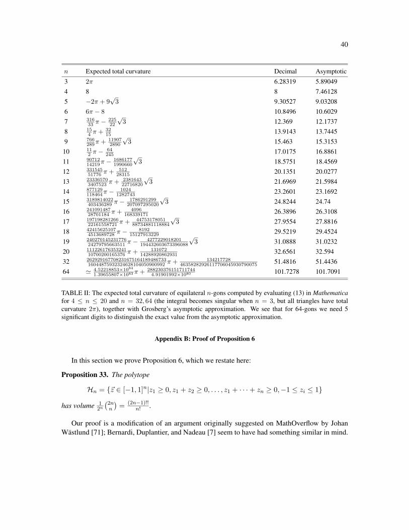
40

n Expected total curvature Decimal Asymptotic

3 2π 6.28319 5.890494 8 8 7.461285 −2π + 9

√3 9.30527 9.03208

6 6π − 8 10.8496 10.60297 316

33 π −22522

√3 12.369 12.1737

8 154 π + 32

15 13.9143 13.74459 766

289π + 119072890

√3 15.463 15.3153

10 112 π −

64245 17.0175 16.8861

11 9071214219π −

16861771990660

√3 18.5751 18.4569

12 33154551776 π + 512

28315 20.1351 20.027713 23336570

3407523 π + 238164322716820

√3 21.6969 21.5984

14 877129118464π −

10241282743 23.2601 23.1692

15 3189814022403436289 π −

1786291299207097295020

√3 24.8244 24.74

16 24109148728701184 π + 4096

168339171 26.3896 26.310817 197198281266

22161558721 π + 4475317805188734881118884

√3 27.9554 27.8816

18 424156251074513689728 π −

819215127913229 29.5219 29.4524

19 24027014523177624279795663511 π −

4277229018201194432603673396088

√3 31.0888 31.0232

20 11122617635324110700200165376 π + 131072

14288920862931 32.6561 32.59432 262929167708231675164189486733

16044875932324628104050900992 π + 13421772846358282926117706045930790075 51.4816 51.4436

64 ' 4.52218853×1084

1.39655807×1083π + 2882303761517117444.91901992×1080 101.7278 101.7091

TABLE II: The expected total curvature of equilateral n-gons computed by evaluating (13) in Mathematicafor 4 ≤ n ≤ 20 and n = 32, 64 (the integral becomes singular when n = 3, but all triangles have totalcurvature 2π), together with Grosberg’s asymptotic approximation. We see that for 64-gons we need 5significant digits to distinguish the exact value from the asymptotic approximation.

Appendix B: Proof of Proposition 6

In this section we prove Proposition 6, which we restate here:

Proposition 33. The polytope

Hn = {~z ∈ [−1, 1]n|z1 ≥ 0, z1 + z2 ≥ 0, . . . , z1 + · · ·+ zn ≥ 0,−1 ≤ zi ≤ 1}

has volume 12n

(2nn

)= (2n−1)!!

n! .

Our proof is a modification of an argument originally suggested on MathOverflow by JohanWastlund [71]; Bernardi, Duplantier, and Nadeau [7] seem to have had something similar in mind.

41

Proof. Suppose that sk(~z) = z1 + · · · + zk is the k-th partial sum of the coordinates of ~z, andby convention we set s0(~z) = 0. The polytope Hn can be defined as the subset of the hypercubewhere all sk(~z) ≥ 0. In the remainder of the hypercube, the subset of ~z where all the sk(~z) aredifferent has full measure: we now partition this set into a collection of n polytopes S0, . . . ,Sndefined by

Sk := {~z ∈ [−1, 1]n −Hn | the smallest si(~z) is sk(~z) }.

We claim that VolSk = VolHk ·VolHn−k for k = 1, . . . , n− 1 and VolSn = VolHn. Considerthe linear map

Lk :Sk ⊂ Rn → Rk × Rn−k, Lk(z1, . . . , zn) = ((−zk,−zk−1, . . . ,−z1), (zk+1, . . . , zn)).

It is clear that this map preserves unsigned volume. We claim the image is exactly Hk × Hn−k.Consider the partial sums of (−zk, . . . ,−z1). The i-th partial sum is given by

si(−zk, . . . ,−z1) = −zk − zk−1 − · · · − zk−i+1 = sk−i(z1, . . . , zn)− sk(z1, . . . , zn).

The point (−zk, . . . ,−z1) is in Hk if and only if this partial sum is positive for alli ∈ {1, . . . , k}. But that happens exactly when sk(~z) is negative9 and the smallest partial sumamong s1(~z), . . . , sk(~z). On the other hand, if we consider the partial sums of (zk+1, . . . , zn), weget

si(zk+1, . . . , zn) = zk+1 + · · ·+ zk+i = sk+i(z1, . . . , zn)− sk(z1, . . . , zn).

The point (zk+1, . . . , zn) is in Hn−k if and only if this partial sum is positive for alli ∈ {1, . . . , n− k}. But that happens exactly when sk(~z) is the smallest partial sum amongsk(~z), . . . , sn(~z), proving the claim. When k = n, Sn is just a reversed and negated copy ofHn itself.

We now have the relation

Vol[−1, 1]n = 2n = VolHn +∑

VolSk

= 2 VolHn +n−1∑k=1

VolHk VolHn−k. (B1)

and we can prove the formula by induction on n.

When n = 1 the polytopeH1 = [0, 1] and so the formula holds. For the inductive step, assumethat VolHk = 1

2k

(2kk

)for all k < n. Then solving (B1) for VolHn yields

VolHn = 2n−1 − 12n+1

n−1∑k=1

(2kk

)(2(n− k)n− k

). (B2)

9 Remember our convention that s0(~z) = 0, which is applied when i = k.

42

Using the Chu-Vandermonde identity

n∑k=0

(x

k

)(y

n− k

)=(x+ y

n

)with x = y = −1/2 and recalling that(

−1/2

m

)= (−1)m

(2mm

)1

22mand

(−1p

)= (−1)p

for any positive integers m and p, we see that

n−1∑k=1

(2kk

)(2(n− k)n− k

)=

n∑k=0

(2kk

)(2(n− k)n− k

)− 2(

2nn

)= 22n − 2

(2nn

).

Therefore, equation (B2) simplifies to

VolHn =12n

(2nn

),

as desired.

[1] Sotero Alvarado, Jorge Alberto Calvo, and Kenneth C Millett. The generation of random equilateralpolygons. Journal of Statistical Physics, 143(1):102–138, 2011.

[2] Hans C Andersen and Persi W Diaconis. Hit and run as a unifying device. Journal de la SocieteFrancaise de Statistique, 148(4):5–28, 2007.

[3] Michael F Atiyah. Convexity and commuting Hamiltonians. Bulletin of the London MathematicalSociety, 14(1):1–15, 1982.

[4] David Avis and Komei Fukuda. A pivoting algorithm for convex hulls and vertex enumeration ofarrangements and polyhedra. Discrete & Computational Geometry, 8(3):295–313, 1992.

[5] Richard Barakat. Isotropic random flights. Journal of Physics A: Mathematical, Nuclear and General,6(6):796, 1973.

[6] Craig J Benham and Steven P Mielke. DNA Mechanics. Annual Review of Biomedical Engineering,7(1):21–53, 2005.

[7] Olivier Bernardi, Bertrand Duplantier, and Philippe Nadeau. A bijection between well-labelled positivepaths and matchings. Seminaire Lotharingien de Combinatoire, 63:Art. B63e–13, 2010.

[8] Julius R Blum and Pramod K Pathak. A Note on the Zero-one Law. Annals of Mathematical Statistics,43(3):1008–1009, 1972.

[9] Arnon Boneh and A Golan. Constraints redundancy and feasible region boundedness by randomfeasible point generator (RGPG) . In Third European Congress on Operations Research - EURO III,Amsterdam, 1979.

43

[10] David Borwein and Jonathan M Borwein. Some remarkable properties of sinc and related integrals.Ramanujan Journal. An International Journal Devoted to the Areas of Mathematics Influenced byRamanujan, 5(1):73–89, 2001.

[11] Michel Brion. Cohomologie equivariante des points semi-stables. Journal fur die Reine und Ange-wandte Mathematik, 421:125–140, 1991.

[12] Aniello Buonocore, Enrica Pirozzi, and Luigia Caputo. A note on the sum of uniform random variables.Statistics and Probability Letters, 79(19):2092–2097, 2009.

[13] Carlos Bustamante, Zev Bryant, and Steven B Smith. Ten years of tension: single-molecule DNAmechanics. Nature, 421:423–426, 2003.

[14] Jorge Alberto Calvo. The embedding space of hexagonal knots. Topology Appl., 112(2):137–174,2001.

[15] Jason Cantarella, Tetsuo Deguchi, and Clayton Shonkwiler. Probability Theory of Random Polygonsfrom the Quaternionic Viewpoint. Communications on Pure and Applied Mathematics, 2013.

[16] Jason Cantarella, Alexander Y Grosberg, Robert B Kusner, and Clayton Shonkwiler. The expectedtotal curvature of random polygons. Preprint, arXiv:1210.6537 [math.DG], 2012.

[17] Francesco Caravenna. A local limit theorem for random walks conditioned to stay positive. ProbabilityTheory and Related Fields, 133(4):508–530, 2005.

[18] Kung Sik Chan and Charles J Geyer. Discussion: Markov Chains for Exploring Posterior Distributions.The Annals of Statistics, 22(4):1747–1758, 1994.

[19] Bernard Chazelle. An optimal convex hull algorithm in any fixed dimension. Discrete & Computa-tional Geometry, 10(4):377–409, 1993.

[20] Robert Cogburn. The central limit theorem for Markov processes. Proc Sixth Berkeley Symp MathStatist Probab, 1972.

[21] Yuanan Diao, Claus Ernst, Anthony Montemayor, Eric J Rawdon, and Uta Ziegler. The knot spectrumof confined random equilateral polygons. University of North Carolina, Charlotte Technical ReportSeries Preprint 2013-15, 2013.

[22] Yuanan Diao, Claus Ernst, Anthony Montemayor, and Uta Ziegler. Generating equilateral randompolygons in confinement. Journal of Physics A: Mathematical and Theoretical, 44(40):405202, 2011.

[23] Yuanan Diao, Claus Ernst, Anthony Montemayor, and Uta Ziegler. Generating equilateral randompolygons in confinement II. Journal of Physics A: Mathematical and Theoretical, 45(27):275203,2012.

[24] Yuanan Diao, Claus Ernst, Anthony Montemayor, and Uta Ziegler. Generating equilateral randompolygons in confinement III. Journal of Physics A: Mathematical and Theoretical, 45(46):465003,2012.

[25] Johannes J Duistermaat and Gerrit J Heckman. On the variation in the cohomology of the symplecticform of the reduced phase space. Inventiones Mathematicae, 69(2):259–268, 1982.

[26] Claus Ernst and Uta Ziegler. Personal Communication.[27] Ewgenij Gawrilow and Michael Joswig. polymake: a framework for analyzing convex polytopes.

In Polytopes—combinatorics and computation (Oberwolfach, 1997), pages 43–73. Birkhauser, Basel,2000.

[28] Charles J Geyer. Practical Markov Chain Monte Carlo. Statistical Science, 7(4):473–483, 1992.[29] Alexander Y Grosberg. Total curvature and total torsion of a freely jointed circular polymer with

n� 1 segments. Macromolecules, 41(12):4524–4527, 2008.[30] Victor Guillemin and Shlomo Sternberg. Convexity properties of the moment mapping. Inventiones

Mathematicae, 67(3):491–513, 1982.[31] Jean-Claude Hausmann and Allen Knutson. Polygon spaces and Grassmannians. L’Enseignement

44

Mathematique. Revue Internationale. 2e Serie, 43(1-2):173–198, 1997.[32] Jean-Claude Hausmann and Allen Knutson. The cohomology ring of polygon spaces. Universite de

Grenoble. Annales de l’Institut Fourier, 48(1):281–321, 1998.[33] Nigel J Hitchin, Anders Karlhede, Ulf Lindstrom, and Martin Rocek. Hyperkahler metrics and super-

symmetry. Communications in Mathematical Physics, 108(4):535–589, 1987.[34] Benjamin Howard, Christopher Manon, and John J Millson. The toric geometry of triangulated poly-

gons in Euclidean space. Canadian Journal of Mathematics. Journal Canadien de Mathematiques,63(4):878–937, 2011.

[35] Barry D Hughes. Random Walks and Random Environments: Volume 1: Random Walks. ClarendonPress, 1995.

[36] Yasuhiko Kamiyama and Michishige Tezuka. Symplectic volume of the moduli space of spatial poly-gons. Journal of Mathematics of Kyoto University, 39(3):557–575, 1999.

[37] Michael Kapovich and John J Millson. The symplectic geometry of polygons in Euclidean space.Journal of Differential Geometry, 44(3):479–513, 1996.

[38] Vu The Khoi. On the symplectic volume of the moduli space of spherical and Euclidean polygons.Kodai Mathematical Journal, 28(1):199–208, 2005.

[39] Frances Clare Kirwan. The cohomology rings of moduli spaces of bundles over Riemann surfaces.Journal of the American Mathematical Society, 5(4):853–906, 1992.

[40] Konstantin V Klenin, Alexander V Vologodskii, Vadim V Anshelevich, Alexander M Dykhne, andMaxim D Frank-Kamenetskii. Effect of excluded volume on topological properties of circular DNA.Journal of Biomolecular Structure and Dynamics, 5(6):1173–1185, 1988.

[41] Krzysztof Łatuszynski, Gareth O Roberts, and Jeffrey S Rosenthal. Adaptive Gibbs samplers andrelated MCMC methods. The Annals of Applied Probability, 23(1):66–98, 2013.

[42] Reginald Douglas Lord. The use of the Hankel transform in statistics I. General theory and examples.Biometrika, 41(1/2):44–55, 1954.

[43] Laszlo Lovasz. Hit-and-run mixes fast. Mathematical Programming. A Publication of the Mathemati-cal Programming Society, 86(3, Ser. A):443–461, 1999.

[44] Laszlo Lovasz and Santosh Vempala. Hit-and-Run from a Corner. SIAM Journal on Computing,35(4):985–1005, 2006.

[45] Rhonald C Lua, Nathan T Moore, and Alexander Y Grosberg. Under-knotted and over-knotted poly-mers: 2. Compact self-avoiding loops. In Jorge Alberto Calvo, Kenneth C Millett, Eric J Rawdon, andAndrzej Stasiak, editors, Physical and Numerical Models in Knot Theory: Including Applications tothe Life Sciences, pages 385–398. World Scientific Publishing Co., Singapore, 2004.

[46] Alessia Mandini. The Duistermaat-Heckman formula and the cohomology of moduli spaces of poly-gons. Journal of Symplectic Geometry, 2013.

[47] Kanti V Mardia and Peter E Jupp. Directional Statistics. Wiley Series in Probability and Statistics.John Wiley & Sons Ltd., Chichester, 2000.

[48] Jean-Luc Marichal and Michael J Mossinghoff. Slices, slabs, and sections of the unit hypercube.Online Journal of Analytic Combinatorics, 3:1–11, 2008.

[49] Jerrold Marsden and Alan Weinstein. Reduction of symplectic manifolds with symmetry. Reports onMathematical Physics, 5(1):121–130, 1974.

[50] Kenneth R Meyer. Symmetries and integrals in mechanics. In Dynamical systems (Proc. Sympos.,Univ. Bahia, Salvador, 1971), pages 259–272. Academic Press, New York, 1973.

[51] Kenneth C Millett. Knotting of regular polygons in 3-space. Journal of Knot Theory and its Ramifica-tions, 3(3):263–278, 1994.

[52] Nathan T Moore and Alexander Y Grosberg. Limits of analogy between self-avoidance and topology-

45

driven swelling of polymer loops. Physical Review E. Statistical Physics, Plasmas, Fluids, and RelatedInterdisciplinary Topics, 72(6):061803, 2005.

[53] Nathan T Moore, Rhonald C Lua, and Alexander Y Grosberg. Topologically driven swelling of apolymer loop. Proceedings of the National Academy of Sciences, 101(37):13431–13435, 2004.

[54] Nathan T Moore, Rhonald C Lua, and Alexander Y Grosberg. Under-knotted and over-knotted poly-mers: 1. Unrestricted loops. In Jorge Alberto Calvo, Kenneth C Millett, Eric J Rawdon, and AndrzejStasiak, editors, Physical and Numerical Models in Knot Theory: Including Applications to the LifeSciences, pages 363–384. World Scientific Publishing Co., Singapore, 2004.

[55] Enzo Orlandini and Stuart G Whittington. Statistical topology of closed curves: Some applications inpolymer physics. Reviews of Modern Physics, 79(2):611–642, 2007.

[56] Xavier Pennec. Intrinsic statistics on Riemannian manifolds: Basic tools for geometric measurements.Journal of Mathematical Imaging and Vision, 25(1):127–154, 2006.

[57] George Polya. On a few questions in probability theory and some definite integrals related to them.PhD thesis, Eotvos Lorand University, 1912.

[58] George Polya. Berechnung eines bestimmten integrals (calculating some definite integrals). Mathe-matisches Annalen, 74:204–212, 1913.

[59] Lord Rayleigh. On the problem of random vibrations, and of random flights in one, two, or threedimensions. Philosophical Magazine Series 5, 37(220):321–347, 1919.

[60] Gareth O Roberts and Jeffrey S Rosenthal. Geometric ergodicity and hybrid Markov chains. ElectronicCommunications in Probability, 2:13–25, 1997.

[61] Wolfgang Sendler. A note on the proof of the zero-one law of Blum and Pathak. The Annals ofProbability, 3(6):1055–1058, 1975.

[62] Robert L Smith. Monte Carlo procedures for generating random feasible solutions to mathematicalprograms. In A Bulletin of the ORSA/TIMS Joint National Meeting, Washington, DC, 1980. Universityof Pittsburgh.

[63] Robert L Smith. Efficient Monte Carlo procedures for generating points uniformly distributed overbounded regions. Operations Research, 32(6):1296–1308, 1984.

[64] Chris Soteros. Personal Communication.[65] Terence R Strick, Vincent Croquette, and David Bensimon. Single-molecule analysis of DNA uncoil-

ing by a type II topoisomerase. Nature, 404(6780):901–904, 2000.[66] Tatsuru Takakura. Intersection theory on symplectic quotients of products of spheres. International

Journal of Mathematics, 12(1):97–111, 2001.[67] Luke Tierney. Markov chains for exploring posterior distributions. Annals of Statistics, pages 1701–

1728, 1994.[68] Leslie Ronald George Treloar. The statistical length of long-chain molecules. Transactions of the

Faraday Society, 42:77–82, 1946.[69] Rocco Varela, Kenneth Hinson, Javier Arsuaga, and Yuanan Diao. A fast ergodic algorithm for gener-

ating ensembles of equilateral random polygons. Journal of Physics A: Mathematical and Theoretical,42(9):095204, 2009.

[70] Alexander V Vologodskii, Vadim V Anshelevich, Alexander V Lukashin, and Maxim D Frank-Kamenetskii. Statistical mechanics of supercoils and the torsional stiffness of the DNA double helix.Nature, 280(5720):294–298, 1979.

[71] Johan Wastlund (mathoverflow.net/users/14302). A random walk with uniformly distributed steps.MathOverflow. http://mathoverflow.net/questions/94262 (version: 2012-04-17).

[72] Gijs JL Wuite, Steven B Smith, Mark Young, David Keller, and Carlos Bustamante. Single-moleculestudies of the effect of template tension on T7 DNA polymerase activity. Nature, 404(6773):103–106,

46

2000.[73] Laura Zirbel and Kenneth C Millett. Characteristics of shape and knotting in ideal rings. Journal of

Physics A: Mathematical and Theoretical, 45(22):225001, 2012.