The Structure of Rooted Weighted Trees Modeling Layered ... · The Structure of Rooted Weighted Trees Modeling Layered Cyber-security Systems Geir Agnarsson, ... The outline of this

Acta Cybernetica 22 (2016) 735–769.

The Structure of Rooted Weighted Trees Modeling

Layered Cyber-security Systems

Geir Agnarsson∗, Raymond Greenlaw†, and Sanpawat Kantabutra‡

Abstract

In this paper we consider the structure and topology of a layered-securitymodel in which the containers and their nestings are given in the form of arooted tree T . A cyber-security model is an ordered three-tuple M = (T,C, P )where C and P are multisets of penetration costs for the containers and target-acquisition values for the prizes that are located within the containers, respec-tively, both of the same cardinality as the set of the non-root vertices of T .The problem that we study is to assign the penetration costs to the edgesand the target-acquisition values to the vertices of the tree T in such a waythat minimizes the total prize that an attacker can acquire given a limitedbudget. The attacker breaks into containers starting at the root of T and oncea vertex has been broken into, its children can be broken into by paying theassociated penetration costs. The attacker must deduct the correspondingpenetration cost from the budget, as each new container is broken into. For agiven assignment of costs and target values we obtain a security system. Weshow that in general it is not possible to develop an optimal security systemfor a given cyber-security model M . We define P- and C-models where thepenetration costs and prizes, respectively, all have unit value. We show thatif T is a rooted tree such that any P- or C-model M = (T,C, P ) has anoptimal security system, then T is one of the following types: (i) a rootedpath, (ii) a rooted star, (iii) a rooted 3-caterpillar, or (iv) a rooted 4-spider.Conversely, if T is one of these four types of trees, then we show that any P-or C-model M = (T,C, P ) does have an optimal security system. Finally, westudy a duality between P- and C-models that allows us to translate resultsfor P-models into corresponding results for C-models and vice versa. The re-sults obtained give us some mathematical insights into how layered-securitydefenses should be organized.

Keywords: cyber-security model, duality, graph minors, rooted tree, secu-rity system, system attack, tree types, weighted rooted tree

∗Department of Mathematical Sciences, George Mason University, Fairfax, VA 22030, E-mail:[email protected]†Department of Cyber Sciences, United States Naval Academy, Annapolis, Maryland 21402,

E-mail: [email protected]‡The Theory of Computation Group, Computer Engineering Department, Chiang Mai Univer-

sity, Chiang Mai, 50200, Thailand, E-mail: [email protected]

DOI: 10.14232/actacyb.22.4.2016.2

736 Geir Agnarsson, Raymond Greenlaw, and Sanpawat Kantabutra

1 Introduction

According to [6], the global cyber-security market cost in 2017 is expected to top120 billion US dollars. This site also reports that there are 18 victims of a cybercrime every single second! Other sources report similarly alarming and worseningstatistics. There is agreement that the number of cyber attacks is increasing rapidly,and the consequences of such attacks are greater than ever on economics, nationalsecurity, and personal data. Threats come from nation states with advanced cyberwarfare commands, nation states having less technical capabilities but intent ondoing harm, ideologically motivated groups of hackers or extremists, profit-seekingcriminals, and others. As a result, quite a bit of work has been done where cyber-security systems, or more generally layered computer systems, are modeled as afixed weighted trees. For example, in [1, 3, 4, 8, 10, 12] the authors consider findingweight-constrained, maximum-density subtrees and similar structures given a fixedweighting of a tree as part of the input. In these cases weights are specified on bothvertices and edges. There has also been some research on network fortification andproblems related to that topic. For example, in [13] stochastic linear programminggames are studied and it is demonstrated how these can, among other things,model certain network fortifications. In [14] the problem of network interdiction isstudied – how to minimize the maximum amount of flow an adversary/enemy canpush through a given network from a source s to a sink t. There each edge/arc isprovided with a fixed integer capacity and an integer resource (required to deletethe edge/arc). This is a variation of the classical Max-Flow-Min-Cut Theorem.Although interesting in their own way, neither of these papers or related papersthat we have found in the literature address directly what we study in this paper.To build secure systems requires first principles of security. “In other words, weneed a science of cyber-security that puts the construction of secure systems onto afirm foundation by giving developers a body of laws for predicting the consequencesof design and implementation choices” [11]. To this end, Schneider called for moremodels and abstractions to study cyber security [11]. This paper is a step in thatdirection. We hope that others will build on this work to develop even better andmore realistic models, overcome the shortcomings of our model, as well as developadditional foundational results.

Building on the work done in [3], in this paper we study a layered-securitymodel and strategies for assigning penetration costs and target-acquisition valuesso as to minimize the amount of damage an attacker can do to a system. That is,we examine security systems. The approach we take here is to assign weights tothe vertices and edges of a tree in order to build a cyber defense that minimizes theamount of prize an attacker can accumulate given a limited budget. To the bestof our knowledge this approach is new in that the usual approach is to consider aparticular weighted tree as input. In [3] the following question was posed: Can onemathematically prove that the intuition of storing high-value targets deeper in thesystem and having higher penetration costs on the outer-most layers of the systemresults in the best or at least good security? In this paper we answer this questionand obtain more general and specific results. We define three types of security

The Structure and Topology of Rooted Weighted Trees . . . 737

systems: improved, good, and optimal. We show that not all cyber-security modelsadmit optimal security systems, but prove that paths and stars do. We define andstudy P- and C-models where all penetration costs, or all prizes, are set to one,respectively. We classify the types of trees that have optimal security systems forboth P- and C-models. We then discuss a duality between P- and C-models, whichprovides a dictionary to translate results for P-models into corresponding resultsfor C-models, and vice versa.

The outline of this article is as follows. In Section 2 we present the rationalefor our layered-security model. In Section 3 we define the framework for securitysystems and present the definitions of improved, good, and optimal security sys-tems, and state some related observations and examples. In Section 4 we exploreoptimal security systems and prove that they do not always exist, but they existif and only if the underlying tree T of the given security system is either a pathrooted at a leaf, or a star rooted at its center vertex. In Section 5 we define P- andC-models and show that any cyber-security model M = (T,C, P ) is equivalent toboth a P-model M ′ and a C-model M ′′. We further show that if T is a rooted treesuch that any P- or C-model M has an optimal security system, then T is one of thefollowing four types: (i) a rooted path, (ii) a rooted star, (iii) a rooted 3-caterpillar,or (iv) a rooted 4-spider. In Section 6 we prove that if T is one of the four typesof rooted trees mentioned above, then any P-model does indeed have an optimalsecurity system. In Section 7 we define a duality between equivalence classes ofP-models and equivalence classes of C-models that serves as a dictionary allowingus to obtain equivalent results for C-models from those of the P-models that wereobtained in Section 6. In particular, we obtain Theorem 7.2 that completely classi-fies which P- and which C-models have optimal security systems. Conclusions andopen problems are discussed in Section 8.

2 Rationale for Our Layered-Security Model

In defining our layered-security model to study defensive cyber security, we need tostrike a balance between simplicity and utility. If the model is too simple, it will notbe useful to provide insight into real situations; if the model is too complex, it willbe too cumbersome to apply, and we may get bogged down in too many details. Themodel described in this paper is a step toward gaining a better understanding of abroad range of security systems in a graph-theoretical setting for a layered-securitymodel.

Many systems contain layered security or what is commonly referred to asdefense-in-depth, where valuable assets are hidden behind many different layersor secured in numerous ways. For example, a host-based defense might layer secu-rity by using tools such as signature-based vendor anti-virus software, host-basedsystems security, host-based intrusion-prevention systems, host-based firewalls, en-cryption, and restriction policies, whereas a network-based defense might providedefense-in-depth by using items such as web proxies, intrusion-prevention systems,firewalls, router-access control lists, encryption, and filters [9]. To break into such


a system and steal a valuable asset requires that several levels of security be pen-etrated, and, of course, there is an associated cost to break into each level, forexample, money spent, time used, or the punishment served for getting caught.

Our model focuses on the layered aspect of security and is intended to capturethe notion that there is a cost associated with penetrating each additional levelof a system and that attackers have finite resources to utilize in a cyber attack.Defenders have the ability to secure targets using defense mechanisms of variousstrengths and to secure targets in desired locations and levels. We assume thatthe structure where targets will be stored, that is, the container nestings; is givenas part of the input in the form of a rooted tree. In this way we can study allpossible structures at a single time, as they can be captured in the definition ofour problems. This methodology is as opposed to having the defender actuallyconstruct a separate defense structure for each input.

For any specific instance of a problem, a defender of a system will obviouslyconsider the exact details of that system and design a layered-security approachto fit one’s actual system. Similarly, a traveling salesman will be concerned aboutconstructing a tour of his particular cities, not a tour of any arbitrary set of citieswith any arbitrary set of costs between pairs of cities. Nevertheless, researchershave found it extremely helpful to consider a general framework in which to studythe Traveling Salesman Problem. And, in studying the general problem,insights have been gained into all instances of the problem. Thus, we believe itis worthwhile to consider having a fixed structure as part of our input, and thisapproach is not significantly different from that used in complexity theory to studyproblems [5, 7].

In this paper we focus on a static defense. We pose as an open problem thequestion of how to create a defense and an attack strategy if the defender is allowedto move targets around dynamically or redistribute a portion of a prize. We alsoconsider the total prize as the sum of the individual values of the targets collectedalthough one could imagine using other or more complex functions of the targetvalues to quantify the damage done by an attacker. Our defensive posture is formedby assigning to the edges and vertices of the rooted tree in question the input-provided penetration costs and target-acquisition values, respectively. We formalizethe model, the notion of a security system, and the concept of a system attack inthe next section.

3 Cyber-Security Model and Security Systems

Let N = {1, 2, 3, . . .}, Q be the rational numbers, and Q+ be the non-negativerational numbers.

Definition 3.1. A cyber-security model (CSM) M is given by a three-tuple M =(T,C, P ), where T is a directed tree rooted at r having n ∈ N non-root vertices, Cis a multiset of penetration costs c1, . . . , cn ∈ Q+, and P is a multiset of target-acquisition-values (or prizes for short) p1, . . . , pn ∈ Q+.


Remark. As mentioned right after Observation5.1, strictly speaking, we couldhave stated the above definition using the set N of natural numbers instead of non-negative rationals Q+ for possible penetrations costs and prizes. We do, however,prefer the most general definition we can discuss.

Throughout V (T ) = {r, u1, . . . , un}, where r is the designated root that indi-cates the start of a system attack, and E(T ) = {e1, . . . , en} denotes the set of edgesof T , where our labeling is such that ui is always the head of the edge ei. Theprize at the root is set to 0. The penetration costs model the expense for breakingthrough a layer of security, and the target-acquisition-values model the amount ofprize one acquires for breaking through a given layer and exposing a target. Thepenetration costs will be weights that are assigned to edges in the tree, and thetarget-acquisition-values, or the prizes, are weights that will be assigned to verticesin the tree.

Sometimes we do not distinguish a target from its acquisition value or prize,nor a container, which is a layer of security, from its penetration cost. Note thatone can think of each edge in the rooted tree as another container, and as onegoes down a path in the tree, as penetrating additional layers of security. We canassume that the number of containers and targets is the same. Since if we havea container housing another container (and nothing else), we can just look at this“double” container as a single container of penetration cost equal to the sum of thetwo nested ones. Also, if a container includes many prizes, we can just lump themall into a single prize, which is the sum of them all.

Recall that in a rooted tree T , each non-root vertex u ∈ V (T ) has exactly oneparent, and that we assume the edges of T are directed naturally away from theroot r in such a way that each non-root vertex has an in-degree of one. The rootis located at level 0 of the tree. Level 1 of the tree consists of the children of theroot, and, in general, level i of the tree consists of the children of those vertices atlevel i− 1 for i ≥ 1. We next present some key definitions about a CSM that willallow us to study questions about security systems.

Definition 3.2. A security system (SS) with respect to a cyber-security modelM = (T,C, P ) is given by two bijections c : E(T ) → C and p : V (T ) \ {r} → P .We denote the security system by (T, c, p).

A system attack (SA) in a security system (T, c, p) is given by a subtree τ of Tthat contains the root r of T .

• The cost of a system attack τ with respect to a security system (T, c, p) isdefined by

cst(τ, c, p) =∑

e∈E(τ)

c(e).

• The prize of a system attack τ with respect to a security system (T, c, p) isdefined by

pr(τ, c, p) =∑

u∈V (τ)

p(u).


• For a given budget B ∈ Q+ the maximum prize pr?(B, c, p) with respect toB is defined by

pr?(B, c, p) :=

max{pr(τ, c, p) : for all system attacks τ ⊆ T, where cst(τ, c, p) ≤ B}.

A system attack τ whose prize is a maximum with respect to a given budgetis called an optimal attack.

The bijection c in Definition 3.2 specifies how difficult it is to break into thevarious containers, and the bijection p specifies the prize associated with a givencontainer. Note that for any SS (T, c, p) we have cst(r, c, p) = 0 ≤ B ∈ Q+. WhenT = ({r},∅), then pr?(B, c, p) = 0 for any B ∈ Q+. When two bijections are givenspecifying a SS, we call the resulting weighted tree a configuration of the CSM. Anyconfiguration represents a defensive posture and hence the name security system.Note that the CSM can be used to model any general security system and not justcyber-security systems. We are interested in configurations that make it difficultfor an attacker to accumulate a large prize. It is natural to ask if a given defensivestance can be improved. Next we introduce the notion of an improved securitysystem that will help us to address this question.

Definition 3.3. Given a CSM M = (T,C, P ) and a SS (T, c, p), an improvedsecurity system (improved SS) with respect to (T, c, p) is a SS (T, c′, p′) such thatfor any budget B ∈ Q+ we have pr?(B, c′, p′) ≤ pr?(B, c, p), and there exists somebudget B′ ∈ Q+ such that pr?(B′, c′, p′) < pr?(B′, c, p).

Definition 3.3 captures the idea of a better placement of prizes and/or penetra-tion costs so that an attacker cannot do as much damage. That is, in an improvedSS one can never acquire a larger overall maximum prize with respect to any bud-get B; and furthermore, there must be at least one particular budget where theattacker actually does worse. Notice that there can be an improved SS (T, c′, p′),where for some budget B ∈ Q+, there is a SA τ whose cost is less than or equal toB for both SSs such that pr(τ, c′, p′) > pr(τ, c, p). In this case an attacker obtainsa larger prize in the improved SS; and, of course, this situation is undesirable andmeans a weaker defense against this specific attack. We, however, are interestedin improved SSs with respect to a given budget rather than a particular SA. Sincewe have exactly n penetration costs and n prizes to assign, it is difficult to imaginean improved SS for all but the most-restricted trees in which all SAs would beimproved in the sense just described. Next, we formalize the notion of an optimalsecurity system.

Definition 3.4. Let M = (T,C, P ) be a given CSM. (i) For a budget B ∈ Q+, aSS (T, c, p) is optimal w.r.t. B if there is no other SS (T, c′, p′) for M such thatpr?(B, c′, p′) < pr?(B, c, p). (ii) (T, c, p) is optimal if it is optimal w.r.t. any budgetB ∈ Q+.

Notice that an optimal SS is not necessarily the best possible. We could definea critically optimal security system to be one where for every single SA the SS was


at least as good as all others and for at least one better. And, in a different context,these SSs might be interesting. However, in light of Theorem 4.1 in the followingsection, which shows that even an optimal SS may not exist for a given CSM, we donot pursue critically optimal SSs further in this paper. By Definitions 3.3 and 3.4we clearly have the following.

Observation 3.1. A SS (T, c, p) for a CSM M = (T,C, P ) is optimal if and onlyif no improved SS for (T, c, p) exists.

We next introduce the concept of two closely-related configurations of a CSM,and this notion will give us a way to relate SSs.

Definition 3.5. Given a CSM M = (T,C, P ), the two configurations (T, c, p), and(T, c′, p′) are said to be neighbors if

1. there exists an edge (u, v) ∈ E(T ) such that

p′(v) = p(u)

p′(u) = p(v)

p′(w) = p(w), otherwise, or

2. there exist two edges (u, v), (v, w) ∈ E(T ) such that

c′((u, v)) = c((v, w))

c′((v, w)) = c((u, v))

c′((x, y)) = c((x, y)), otherwise.

The notion of neighboring configurations will be useful in developing algorithmsfor finding good security systems, which we define next.

Definition 3.6. A good security system (good SS) is a SS (T, c, p) such that noneighboring configuration results in an improved security system.

Given a SS (T, c, p) for a CSM M , a natural question to pose is whether alocal change to the SS can be made in order to strengthen the SS, that is, makethe resulting SS improved. In a practical setting one may not be able to redo thesecurity of an entire system, but instead may be able to make local changes.

Suppose (u, v) ∈ E(T ) where p(u) ≥ p(v), and let p′ be the prize assignmentobtained from p by swapping the prizes on u and v, that is p′(u) = p(v), p′(v) =p(u), and p′(w) = p(w) otherwise. If now τ is any SA, then pr(τ, c, p′) = pr(τ, c, p) ifeither both u, v ∈ V (τ) or neither u nor v are vertices of τ , or pr(τ, c, p′) ≤ pr(τ, c, p)if u ∈ V (τ) and v 6∈ V (τ). In either case pr(τ, c, p′) ≤ pr(τ, c, p) and therefore wehave for any budget B that

pr?(B, c, p′) ≤ pr?(B, c, p). (1)

Similarly, if (u, v), (v, w) ∈ E(T ) where c((u, v)) ≤ c((v, w)), let c′ be the costassignment obtained from c by swapping the costs on the incident edges (u, v) and


(v, w) and leave all the other edge-costs unchanged, that is c′((u, v)) = c((v, w)),c′((v, w)) = c((u, v)) and c′(e) = c(e) otherwise. If τ is a SA, then clearly wealways have pr(τ, c′, p) = pr(τ, c, p). Also, if either both (u, v), (v, w) ∈ E(τ) orneither (u, v) nor (v, w) are edges in τ , then cst(τ, c′, p) = cst(τ, c, p), and if (u, v) ∈E(τ) and (v, w) 6∈ E(τ), then cst(τ, c′, p) ≥ cst(τ, c, p). In either case we havecst(τ, c′, p) ≥ cst(τ, c, p). Hence, if B is any budget, then by mere definition wehave that

pr?(B, c′, p) ≤ pr?(B, c, p). (2)

By (1) and (2) we have the following proposition.

Proposition 3.1. Let M = (T,C, P ) be a CSM. A SS given by (T, c, p) is a goodSS if for all (u, v), (v, w) ∈ E we have c((u, v)) ≥ c((v, w)) and for all non-rootvertices u, v ∈ V (T ) with (u, v) ∈ E(T ) we have p(u) ≤ p(v).

Note that Proposition 3.1 says that on any root to leaf path in T the penetrationcosts occur in decreasing order and the prizes occur in increasing order.

From any configuration resulting from a SS (T, c, p) for a CSM, Proposition 3.1gives a natural O(n2) algorithm for computing a good SS by repeatedly moving toimproved neighboring configurations until no more such neighboring configurationsexist. We can do better than this method by first sorting the values in C and Pusing O(n log n) time, and then conducting a breath-first search of T in O(n) time.We can then use the breath-first search level numbers to define bijections c and pthat meet the conditions of a good SS. We summarize in the following.

Observation 3.2. Given a CSM M = (T,C, P ), there is an O(n log n) algorithmfor computing a good SS for M .

If we could eliminate the sorting step, we would have a more efficient algorithmfor obtaining a good SS, or if we restricted ourselves to inputs that could be sortedin O(n) time. Also, notice that a good SS has the heap property, if we ignore theroot. However, in our case we cannot “choose” the shape of the heap, but we mustuse the structure that is given to us as part of our input.

Suppose that our SS (T, c, p) for M satisfies a strict inequality p(u) > p(v)for some (u, v) ∈ E(T ), or that c((u, v)) < c((v, w)) for some incident edges(u, v), (v, w) ∈ E(T ). A natural question is whether the prize and cost assign-ments p′ and c′ as in (1) and (2) will result in an improved SS as in Definition 3.3.In Example 3.1 we will see that that is not the case.

Convention: Let Tp(`) denote the rooted tree whose underlying graph is apath on 2`+ 1 vertices V (Tp(`)) = {r, u1, . . . , u2`} and directed edges

E(Tp(`)) = {(r, u1), (r, u2), (u1, u3), (u2, u4), . . . , (u2`−3, u2`−1), (u2`−2, u2`)}

rooted at its center vertex. We label the edges by the same index as their heads:e1 = (r, u1), e2 = (r, u2),..., e2`−1 = (u2`−3, u2`−1), and e2` = (u2`−2, u2`), seeFigure 1.

Example 3.1.


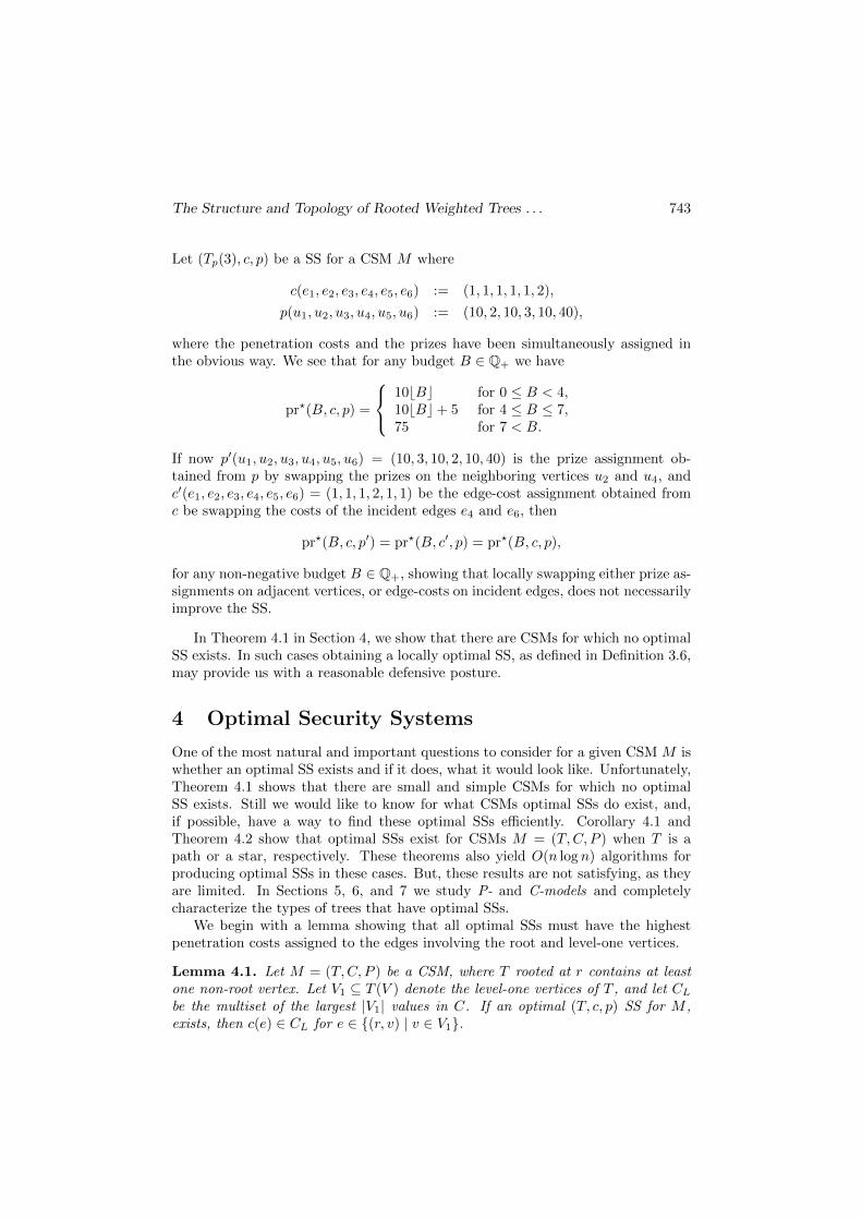
Let (Tp(3), c, p) be a SS for a CSM M where

c(e1, e2, e3, e4, e5, e6) := (1, 1, 1, 1, 1, 2),

p(u1, u2, u3, u4, u5, u6) := (10, 2, 10, 3, 10, 40),

where the penetration costs and the prizes have been simultaneously assigned inthe obvious way. We see that for any budget B ∈ Q+ we have

pr?(B, c, p) =

10bBc for 0 ≤ B < 4,10bBc+ 5 for 4 ≤ B ≤ 7,75 for 7 < B.

If now p′(u1, u2, u3, u4, u5, u6) = (10, 3, 10, 2, 10, 40) is the prize assignment ob-tained from p by swapping the prizes on the neighboring vertices u2 and u4, andc′(e1, e2, e3, e4, e5, e6) = (1, 1, 1, 2, 1, 1) be the edge-cost assignment obtained fromc be swapping the costs of the incident edges e4 and e6, then

pr?(B, c, p′) = pr?(B, c′, p) = pr?(B, c, p),

for any non-negative budget B ∈ Q+, showing that locally swapping either prize as-signments on adjacent vertices, or edge-costs on incident edges, does not necessarilyimprove the SS.

In Theorem 4.1 in Section 4, we show that there are CSMs for which no optimalSS exists. In such cases obtaining a locally optimal SS, as defined in Definition 3.6,may provide us with a reasonable defensive posture.

4 Optimal Security Systems

One of the most natural and important questions to consider for a given CSM M iswhether an optimal SS exists and if it does, what it would look like. Unfortunately,Theorem 4.1 shows that there are small and simple CSMs for which no optimalSS exists. Still we would like to know for what CSMs optimal SSs do exist, and,if possible, have a way to find these optimal SSs efficiently. Corollary 4.1 andTheorem 4.2 show that optimal SSs exist for CSMs M = (T,C, P ) when T is apath or a star, respectively. These theorems also yield O(n log n) algorithms forproducing optimal SSs in these cases. But, these results are not satisfying, as theyare limited. In Sections 5, 6, and 7 we study P- and C-models and completelycharacterize the types of trees that have optimal SSs.

We begin with a lemma showing that all optimal SSs must have the highestpenetration costs assigned to the edges involving the root and level-one vertices.

Lemma 4.1. Let M = (T,C, P ) be a CSM, where T rooted at r contains at leastone non-root vertex. Let V1 ⊆ T (V ) denote the level-one vertices of T , and let CLbe the multiset of the largest |V1| values in C. If an optimal (T, c, p) SS for M ,exists, then c(e) ∈ CL for e ∈ {(r, v) | v ∈ V1}.


Proof. Suppose we have an optimal SS (T, c, p) that does not meet the conditionsof the lemma. Let cs 6∈ CL be the smallest penetration cost assigned by c to anedge between the root r and a vertex vs ∈ V1, that is, c((r, vs)) = cs ≤ c((r, v)) forall v ∈ V1 − {vs}. Let es = (r, vs) and let el be an edge not between the root anda level-one vertex where c(el) ∈ CL. We know that such an edge exists because(T, c, p) does not meet the conditions of the lemma. To show that (T, c, p) cannot bean optimal SS, we define a SS (T, c′, p) by letting c′(es) = c(el), c

′(el) = c(es), andc′(e) = c(e) otherwise. Notice that for the budget B = cs, we have pr?(B, c, p) =p(vs) > 0 = pr?(B, c′, p). This fact contradicts that (T, c, p) is an optimal SS.

If an optimal SS exists, Lemma 4.1 tells us something about its form. In thenext theorem we show that there are CSMs for which no optimal SS exists.

Theorem 4.1. There is a CSM M = (T,C, P ) for which no optimal securitysystem exists.

Proof. Consider M = (T, {1, 2, 3}, {1, 2, 3}), Where T is the tree given by V (T ) ={r, u1, u2, u3} and E(T ) = {e1, e2, e3} where e1 = (r, u1), e2 = (r, u2), and e3 =(u1, u3). By Lemma 4.1 we know that an optimal SS (T, c, p) has c(e3) = 1, andwe can further assume that p(u3) = 3. By considering the budget of B = 2, wecan also assume the prize of the head of the edge of cost 2 to by 1. Therefore, wehave only two possible optimal SSs for M : (T, c, p) with c(e1, e2, e3) = (3, 2, 1) andp(u1, u2, u3) = (2, 1, 3), or (T, c′, p′) with c′(e1, e2, e3) = (2, 3, 1) and p′(u1, u2, u3) =(1, 2, 3), see Figure 2. Since pr?(3, c, p) = 2 and pr?(3, c′, p′) = 4, we see that(T, c′, p′) is not optimal, and since pr?(4, c, p) = 5 and pr?(4, c′, p′) = 4, we see that(T, c, p) is not optimal either. Hence, no optimal SS for M exists.

Although Theorem 4.1 showed that there are CSMs for which no optimal SSexists, we are interested in finding out for which trees T optimal SSs do exist. Weshould point out that the values of the weights in C and P also play an importantrole in whether or not an optimal SS exists for a given tree. In the next theoremwe show that an optimal SS exists for CSMs in which the tree in the model is apath, and this result is independent of the values of the weights in C and P .

Consider a CSM M = (T,C,M) where T is a path rooted at a leaf, so

V (T ) = {u0, u1, . . . , un}, E(T ) = {e1, . . . , en}, (3)

where u0 = r and ei = (ui−1, ui), for each i ∈ {1, . . . , n}. For a SS (T, c, p) for M ,then for convenience let pi = p(ui) and ci = c(ei) for each i. If we have pi ≤ pi+1

and ci ≥ ci+1 for each i ∈ {1, . . . , n − 1} (so the prizes are ordered increasinglyand the edge-costs decreasingly as we go down the path from the root), then byProposition 3.1 the SS (T, c, p) is a good SS as in Definition 3.6. But, we can sayslightly more here when T is a path, in terms of obtaining an improved SS as inDefinition 3.3.

Lemma 4.2. Let M = (T,C,M) be a CSM where T is a path with its vertices andedges labeled as in (3).


r

u1 u2

u3 u4

u5 u6

e1 e2

e3 e4

e5 e6

Tp(3)

Figure 1: Tp(3) is a path on seven vertices rooted at its center.

r

2 1

3

3 2

1

(T, c, p)

r

1 2

3

2 3

1

(T, c′, p′)

Figure 2: Only two possible SSs for M = (T, {1, 2, 3}, {1, 2, 3}).


(i) If (T, c, p) is a SS for M and there is an i with pi > pi+1 and ci+1 > 0, thenthe SS (T, c, p′) where p′ is obtained by swapping the prizes on ui and ui+1 is animproved SS.

(ii) If (T, c, p) is a SS for M and there is an i with ci < ci+1, then the SS(T, c′, p) where c′ is obtained by swapping the edges costs on ei and ei+1 is animproved SS.

Proof. By Proposition 3.1 we only need to show (i) there is a budget B′ suchthat pr?(B′, c, p′) < pr?(B′, c, p) and (ii) a budget B′′ such that pr?(B′′, c′, p) <pr?(B′′, c, p). For each j let τj = T [e1, . . . , ej ] be the rooted sub-path of T thatcontains the first j edges of T .

For B′ = c1 + · · ·+ ci we clearly have

pr?(B′, c, p′) = pr(τi, c, p′)

= p1 + · · ·+ pi−1 + pi+1

< p1 + · · ·+ pi

= pr(τi, c, p)

= pr?(B′, c, p),

showing that (T, c, p′) is an improved SS for M .Likewise, we have

pr?(B′, c′, p) = pr(τi−1, c′, p)

= p1 + · · ·+ pi−1

< p1 + · · ·+ pi

= pr(τi, c, p)

= pr?(B′, c, p),

showing that (T, c′, p) is also an improved SS for M .

Given any SS (T, c, p) for M as in Lemma 4.2 when T is a rooted path, by bubblesorting the prizes and the edge costs increasingly and decreasingly respectively, aswe go down the path T from the root, we obtain by Lemma 4.2 a SS (T, c′, p′) suchthat for any budget B we have pr?(B, c′, p′) ≤ pr?(B, c, p). We therefore have thefollowing corollary.

Corollary 4.1. If M = (T,C,M) is a CSM where T is a rooted path with itsvertices and edges labeled as in (3), then there is an optimal SS for M , and it isgiven by assigning the penetration costs to the edges and the prizes to the verticesin a decreasing order and increasing order respectively from the root.

We now show that an optimal SS exists for M = (T,C, P ) when T is a star.Let T be a star with root r and non-root vertices u1, . . . , nn and edges ei = (r, ui)for i = 1, . . . , n. Suppose the costs and prizes are given by C = {c1, . . . , cn} andP = {p1, . . . , pn}. When considering an arbitrary security system (T, c, p) wherec(ui) = ci and p(ei) = pi for each i, we can without loss of generality assume theedge-costs to be in an increasing order c1 ≤ · · · ≤ cn.


Lemma 4.3. Suppose T is a star and (T, c, p) is a SS as above. If p′ is anotherprize assignment obtained from p by swapping the prizes pi and pj where i < j andpi ≤ pj, then for any budget B we have pr?(B, c, p) ≤ pr?(B, c, p′).

Proof. Let B be a given budget and τ ⊆ T an optimal attack with respect to p, sopr(τ, c, p) = pr?(B, c, p). We consider the following cases.

Case one: If both of ui and uj are in τ , or neither of them are, then we haefpr?(B, c, p) = pr(τ, c, p) = pr(τ, c, p′) ≤ pr?(B, c, p′).

Case two: If ui ∈ V (τ) and uj 6∈ V (τ), then pr?(B, c, p) = pr(τ, c, p) ≤pr(τ, c, p)− pi + pj = pr(τ, c, p′) ≤ pr?(B, c, p′).

Case three: If ui 6∈ V (τ) and uj ∈ V (τ), then τ ′ = (τ − uj) ∪ ui is a rootedsubtree of T with c(τ ′) = c(τ)− cj + ci ≤ B and is therefore within the budget B.Hence, pr?(B, c, p) = pr(τ, c, p) = pr(τ ′, c, p′) ≤ pr?(B, c, p′).

Therefore, in all cases we have pr?(p, c, B) ≤ pr?(p′, c, B).

Since any permutation is a composition of transpositions, we have the followingtheorem as a corollary.

Theorem 4.2. Let M = (T,C, P ) be a CSM where T is a star rooted at its centervertex. Then there is an optimal SS for M , and it is given by assigning the prizesto the vertices in the same increasing order as the costs are assigned increasinglyto the corresponding edges.

For rooted trees on n non-root vertices, Corollary 4.1 and Theorem 4.2 give riseto natural sorting-based O(n log n) algorithms for computing optimal SSs. Noticethat in an optimal SS in a general tree, the smallest prize overall must be assignedto a level-one vertex u which has the largest penetration cost assigned to its corre-sponding edge, (r, u), to the root. And, furthermore, we cannot say more than thisstatement for arbitrary trees as the next assignment of a prize will depend on therelative values of the penetration costs, prizes, and structure of the tree. In viewof the fact that optimal SSs do not exist, except for paths and stars as we will seeshortly in Observation 5.1, we turn our attention to restricted CSMs and classifythem with respect to optimal SSs.

5 Specific Security Systems, P-Models,and C-Models

In this section we extend CSMs to include penetration costs and prizes of valuezero. For a CSM M = (T,C, P ) with no optimal SS and a rooted super-tree T † ofwhich T is a rooted subtree, we can always assign the prize of zero to the nodes inV (T †)\V (T ) and likewise the penetration cost of zero to the edges in E(T †)\E(T ),thereby obtaining a CSM M† = (T †, C†, E†) that also has no optimal SS. Notethat if T is the rooted tree in the proof of Theorem 4.1, then the only rooted treesthat do not have T as a rooted subtrees are paths rooted at one of their leaves orstars rooted at their center vertices. Hence, by the example provided in the proofof Theorem 4.1, we have the following observation.


Observation 5.1. If T is a rooted tree, such that for any multisets C and P ofpenetration costs and prizes, respectively, the CSM M = (T,C, P ) has an optimalSS, then T is either a path rooted at one of its leaves, or a star rooted at its centervertex.

In light of Observation 5.1, we seek some natural restrictions on our CSM Mthat will guarantee it having an optimal SS. Since both the penetration costs andthe prizes of M = (T,C, P ) take values in Q+ we can, by an appropriate scaling,obtain an equivalent CSM where both the costs and prizes take values in N ∪ {0},that is, we may assume c(e) ∈ N ∪ {0} and p(u) ∈ N ∪ {0} for every e ∈ E(T ) andu ∈ V (T ), respectively.

First, we consider the restriction on a CSM M = (T,C, P ) where C consistsof a single penetration-cost value, that is, C = {1, 1, . . . , 1} consists of n copiesof the unit penetration cost one. From a realistic point of view, this assumptionseems to be reasonable; many computer networks consist of computers with similarpassword/encryption security systems on each computer (that is, the penetrationcost is the same for all of the computers), whereas the computers might store dataof vastly distinct values (that is, the prizes are distinct).

Convention: In what follows, it will be convenient to denote the multisetcontaining n (or an arbitrary number of) copies of 1 by I. In a similar way, wewill denote by 1 the map that maps each element of the appropriate domain to 1.As the domain of 1 should be self-evident each time, there should be no ambiguityabout it each time.

Definition 5.1. A P-model is a CSM M = (T, I, P ) where T has n non-rootvertices and where I is constant, consisting of n copies of the unit penetration cost.

Consider a SS (T, c, p) of a CSM M = (T,C, P ). We can obtain an equivalentSS (T ′,1, p′) of a P-model M ′ = (T ′, I, P ′) in the following way: for each edgee = (u, v) ∈ E(T ) with penetration cost c(e) = k ∈ N and prizes p(u), p(v) ∈ N ofits head and tail, respectively, replace the 1-path (u, e, v) with a directed path ofnew vertices and edges (u, e1, u1, e2, u2, . . . , uk−1, ek, v) of length k. We extend thepenetration cost and prize functions by adding zero-prize vertices where needed,that is, 1(f) = 1 for each f ∈ E(T ′), and we let

p′(u) = p(u), p′(v) = p(v), and p′(u1) = p′(u2) = · · · = p′(uk−1) = 0.

In this way we obtain a SS (T ′, c′, p′) of a P-model M ′ = (T ′, I, P ′). We view thevertices V (T ) of positive prize as a subset of V (T ′) (namely, those vertices of T ′

with positive prize).1

Recall that T is a rooted contraction of T ′ if T is obtained from T ′ by a sequenceof simple contractions of edges, and where any vertex contracted into the rootremains the root. This means precisely that T is a rooted minor of T ′ [2, p. 54].

1Note that there are some redundant definitions on the prizes of the vertices when consideringincident edges, but the assignments do agree, as they have the same prize values as in T .


Proposition 5.1. Any SS (T, c, p) of a CSM M = (T,C, P ) is equivalent to a SS(T ′,1, p′) of a P-model M ′ = (T ′, I, P ′) where (i) T is rooted minor of T ′, and (ii)p′(u) = p(u) for each u ∈ V (T ) ⊆ V (T ′), and p′(u) = 0, otherwise.

Proof. (Sketch) Given a budget B ∈ Q+, clearly any optimal attack τ on a SS(T, c, p) with pr(τ, c, p) = pr?(B, c, p) has an equivalent attack τ ′ on a SS (T ′,1, p′)of the same cost cst(τ ′,1, p′) = cst(τ, c, p) and hence within the budget B, where τ ′

is the smallest subtree of T ′ that contains all of the vertices of τ . By construction,we also have that pr(τ ′,1, p′) = pr(τ, c, p) = pr?(B, c, p) since all of the verticesfrom τ are in τ ′ and have the same prize there, and the other vertices in τ ′ haveprize zero. This shows that pr?(B, c, p) ≤ pr?(B,1, p′).

Conversely, an optimal attack τ ′ on (T ′,1, p′) with pr(τ ′,1, p′) = pr?(B,1, p′)yields an attack τ on (T, c, p) by letting τ be the subtree of T induced by the verticesV (τ ′) ∩ V (T ). In this way pr(τ, c, p) = pr(τ ′,1, p′) and cst(τ, c, p) ≤ cst(τ ′,1, p′),since some of the vertices of τ ′ might have zero prize, as they are not in τ . Bydefinition of pr?(·) we have that pr?(B,1, p′) ≤ pr?(B, c, p). Hence, the SS (T, c, p)and (T ′,1, p′) are equivalent.

Secondly, and dually, we can restrict our attention to the case where the multisetof prizes P consists of a single unit prize value, so P = I = {1, 1, . . . , 1} consists ofn copies of the unit prize.

Definition 5.2. A C-model is a CSM M = (T,C, I), where T has n non-rootvertices and where I is constant, consisting of n copies of the unit prize.

As before, consider a SS (T, c, p) of a CSM M = (T,C, P ). We can obtainan equivalent SS (T ′′, c′′,1) of a C-model M ′′ = (T ′′, C ′′, I) in the following way:for each edge e = (u, v) ∈ E(T ) with penetration cost c(e) = k ∈ N and prizesp(u), p(v) ∈ N of its head and tail, respectively, replace the 1-path (u, e, v) with adirected path of new vertices and edges (u, e, u1, e1, u2, . . . , uk−1, ek−1, v) of lengthk. We extend the penetration cost and prize functions by adding zero-cost edgeswhere needed, that is, 1(w) = 1 for every w ∈ V (T ′′), and we let

c′′(e) = c(e) and c′′(e1) = c′′(e2) = · · · = c′′(ek−1) = 0.

In this way we obtain a SS (T ′′, c′′,1) of a C-model M ′′ = (T ′′, C ′′, I), where themultiset of prizes consists of a single unit prize value (

∑u∈V (T )\{r} p(u) copies

of it). We also view the edges E(T ) of positive penetration cost as a subset ofE(T ′′) (namely, those edges of T ′′ with positive penetration cost). We also havethe following proposition that is dual to Proposition 5.1.

Proposition 5.2. Any SS (T, c, p) of a CSM M = (T,C, P ) is equivalent to a SS(T ′′, c′′,1) of a C-model M ′′ = (T ′′, C ′′, I), where (i) T is rooted minor of T ′′, and(ii) c′′(e) = c(e) for each e ∈ E(T ) ⊆ E(T ′′), and c′′(e) = 0, otherwise.

Proof. (Sketch) Suppose we are given a budget B ∈ Q+ and an optimal attack τ ona SS (T, c, p) with pr(τ, c, p) = pr?(B, c, p). Here (T ′′, c′′,1) has an equivalent attack


τ ′′, where τ ′′ is the largest subtree of T ′′ that contains all of the edges of τ and noother edges of T . Note that cst(τ ′′, c′′,1) = cst(τ, c, p) since all of the additionaledges of τ ′′ that are not in V (τ) have zero penetration cost, and so τ ′′ is within thebudget B. Also, by construction we have pr(τ ′′, c′′,1) = pr(τ, c, p) = pr?(B, c, p).This result shows that pr?(B, c, p) ≤ pr?(B, c′′,1).

Conversely, consider an optimal attack τ ′′ on (T ′′, c′′,1) with pr(τ ′′, c′′,1) =pr?(B, c′′,1). By the optimality of τ ′′, every leaf of τ ′′ is a tail of an edge of T , sinceotherwise we can append that edge (of zero penetration cost), and thereby obtainan attack with a prize strictly more than pr(τ ′′, c′′,1), a contradiction. The edgesE(τ ′′) ∩ E(T ) induce a subtree τ of T of the same cost cst(τ, c, p) = cst(τ ′′, c′′,1);and moreover, τ ′′ is, by its optimality, the largest subtree of T ′′ that containsexactly all of the edges of τ , and so pr(τ, c, p) = pr(τ ′′, c′′,1) = pr?(B, c′′,1). Thisresult shows that pr?(B, c′′,1) ≤ pr?(B, c, p). This proves that the SS (T, c, p) and(T ′′, c′′,1) are equivalent.

We now present some examples of both P- and C-models that will play a pivotalrole in our discussion to come.

Definition 5.3. Let T (2) denote the rooted tree given as follows:

V (T (2)) = {r, u1, u2, u3, u4, u5},E(T (2)) = {(r, u1), (r, u2), (u1, u3), (u2, u4), (u2, u5)}.

Note that T (2) has all of its non-root vertices on two non-zero levels. Similarly, letT (3) denote the rooted tree given as follows:

V (T (3)) = {r, u1, u2, u3, u4},E(T (3)) = {(r, u1), (r, u2), (u2, u3), (u3, u4)}.

Note that T (3) has all of its vertices on three non-zero levels.

Convention: For convenience we label the edges of both T (2) and T (3) withthe same index as their heads (see Figures 3 and 4):

T (2) : e1 = (r, u1), e2 = (r, u2), e3 = (u1, u3), e4 = (u2, u4), e5 = (u2, u5).

T (3) : e1 = (r, u1), e2 = (r, u2), e3 = (u1, u3), e4 = (u3, u4).

Example 5.1.

Consider a P-model (with c = 1) on the rooted tree T (2), where the prize valuesare given by P = {0, 1, 2, 2, 3}.

Prize Assignment (A): Consider the case where the prizes have been simultane-ously assigned to the non-root vertices of T (2) by p(u1, u2, u3, u4, u5) := (0, 1, 3, 2, 2)in the obvious way. We will use a similar shorthand notation later for the bijectionc. In this case we see that for budgets of B = 2, 3, we have pr?(2,1, p) = 3 andpr?(3,1, p) = 5, respectively.


r

u1 u2

u3 u4 u5

e1 e2

e3 e4 e5

T (2)

Figure 3: T (2) has all of its non-root vertices on two non-zero levels.

r

u1 u2

u3

u4

e1 e2

e3

e4

T (3)

Figure 4: T (3) has all of its non-root vertices on three non-zero levels.


Prize Assignment (B): Consider now the case where the prizes have been si-multaneously assigned to the non-root vertices of T (2) by p′(u1, u2, u3, u4, u5) :=(1, 0, 3, 2, 2). In this case we see that for the same budgets of B = 2, 3 as in (A),we have pr?(2,1, p′) = 4 and pr?(3,1, p′) = 4, respectively.

From these assignments we see that for budget B = 2, the SS in (A) is betterthan the one in (B), and for B = 3, the SS in (B) is better than the one in (A).

Example 5.2.

Consider a P-model on the rooted tree T (3), where the prize values are given byP = {0, 0, 1, 1}.

Prize Assignment (A): Consider the case where the prizes have been simulta-neously assigned to the non-root vertices of T (3) by p(u1, u2, u3, u4) := (0, 0, 1, 1).In this case we see that for budgets of B = 1, 3, we have pr?(1,1, p) = 0 andpr?(3,1, p) = 2, respectively.

Prize Assignment (B): Consider now the case where the prizes have been simul-taneously assigned to the non-root vertices of T (3) by p′(u1, u2, u3, u4) := (1, 0, 0, 1).In this case we see that for the same budgets of B = 1, 3 as in (A), we havepr?(1,1, p′) = 1 and pr?(3,1, p′) = 1, respectively.


Considering the budget B = 1 for the P-model in Example 5.1, we see that inorder for a prize assignment to be optimal we must have the prizes of u1 and u2to be 0 and 1. Considering further B = 2 we see that an optimal prize assignmentin this case must be p or p′ as in Example 5.1, or p′′ where p′′(u1, u2, u3, u4, u5) :=(1, 0, 2, 3, 2). Since pr?(B,1, p′′) = pr?(B,1, p) for any B, we see that the P-modelin Example 5.1 has no optimal SS. As the P-model in Example 5.2 can be analysedin the same way, we have the following observation.

Observation 5.2. For general prize values P , neither of the P-models M =(T (2), I, P ) nor M = (T (3), I, P ) have optimal SSs.

We will now consider the dual cases of the C-models.

Example 5.3.

Consider a C-model (with p = 1) on the rooted tree T (2), where the penetrationcosts are given by C = {0, 1, 1, 2, 3}.

Cost Assignment (A): Consider the case where the penetration costs have beensimultaneously assigned to the edges of T (2) by c(e1, e2, e3, e4, e5) := (3, 2, 0, 1, 1).In this case we see that for budgets of B = 2, 4, we have pr?(2, c,1) = 1 andpr?(4, c,1) = 3, respectively.

Cost Assignment (B): Consider now the case where the penetration costs havebeen assigned to the edges of T (2) by c′(e1, e2, e3, e4, e5) := (2, 3, 0, 1, 1). In thiscase we see that for the same budgets of B = 2, 4 as in (A), we have pr?(2, c′,1) = 2and pr?(4, c′,1) = 2, respectively.



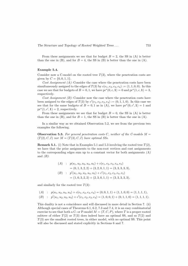
Example 5.4.

Consider now a C-model on the rooted tree T (3), where the penetration costs aregiven by C = {0, 0, 1, 1}.

Cost Assignment (A): Consider the case where the penetration costs have beensimultaneously assigned to the edges of T (3) by c(e1, e2, e3, e4) := (1, 1, 0, 0). In thiscase we see that for budgets of B = 0, 1, we have pr?(0, c,1) = 0 and pr?(1, c,1) = 3,respectively.

Cost Assignment (B): Consider now the case where the penetration costs havebeen assigned to the edges of T (3) by c′(e1, e2, e3, e4) := (0, 1, 1, 0). In this case wesee that for the same budgets of B = 0, 1 as in (A), we have pr?(0, c′,1) = 1 andpr?(1, c′,1) = 2, respectively.


In a similar way as we obtained Observation 5.2, we see from the previous twoexamples the following.

Observation 5.3. For general penetration costs C, neither of the C-models M =(T (2), C, I) nor M = (T (3), C, I) have optimal SSs.

Remark 5.1. (i) Note that in Examples 5.1 and 5.3 involving the rooted tree T (2),we have that the prize assignments to the non-root vertices and cost assignmentsto the corresponding edges sum up to a constant vector for both assignments (A)and (B):

(A) : p(u1, u2, u3, u4, u5) + c(e1, e2, e3, e4, e5)

= (0, 1, 3, 2, 2) + (3, 2, 0, 1, 1) = (3, 3, 3, 3, 3),

(B) : p′(u1, u2, u3, u4, u5) + c′(e1, e2, e3, e4, e5)

= (1, 0, 3, 2, 2) + (2, 3, 0, 1, 1) = (3, 3, 3, 3, 3),

and similarly for the rooted tree T (3):

(A) : p(u1, u2, u3, u4) + c(e1, e2, e3, e4) = (0, 0, 1, 1) + (1, 1, 0, 0) = (1, 1, 1, 1),

(B) : p′(u1, u2, u3, u4) + c′(e1, e2, e3, e4) = (1, 0, 0, 1) + (0, 1, 1, 0) = (1, 1, 1, 1).

This duality is not a coincidence and will discussed in more detail in Section 7. (ii)Although special cases of Theorems 6.1, 6.2, 7.3 and 7.4, it is an easy combinatorialexercise to see that both a C- or P-model M = (T,C, P ), where T is a proper rootedsubtree of either T (2) or T (3) does indeed have an optimal SS, and so T (2) andT (3) are the smallest rooted trees, in either model, with no optimal SS. This pointwill also be discussed and stated explicitly in Sections 6 and 7.


Consider now a given rooted tree T and another rooted tree T † containing Tas a rooted subtree, so T ⊆ T †. Assume that the P-model M = (T, I, P ) has nooptimal SS. Extend M to a P-model on T † by adding a zero prize for each vertex inV (T †)\V (T ), so P † = P ∪Z, where Z is the multiset consisting of |V (T †)|−|V (T )|copies of 0. In this case we have the following.

Observation 5.4. If M = (T, I, P ) is a P-model with no optimal SS, and T †

contains T as a rooted subtree, then the P-model M† = (T †, I, P †) has no optimalSS.

Proof. (Sketch) For any budget consisting of B = m edges and a SS (T,1, p), thereis a rooted subtree τ of T with m edges such that pr(τ,1, p) = pr?(m,1, p). Let1 and p† be the obvious extensions of 1 and p to T †, by letting 1(e) = 1 for alle ∈ E(T †) and p†(u) = 0 for any u ∈ V (T †) \ V (T ). If τ ′ is a rooted subtree ofT † with m edges, then τ ′ ∩ T is a rooted subtree of both T and T † on m or feweredges. Since any vertex of V (τ ′) \ V (T ) has zero prize, we have

pr(τ ′,1, p†) = pr(τ ′ ∩ T,1, p†) = pr(τ ′ ∩ T,1, p) ≤ pr?(m,1, p),

with equality for τ ′ = τ since τ ⊆ T ⊆ T †. Hence, pr?(m,1, p†) = pr?(m,1, p),and we conclude that if M = (T, I, P ) has no optimal SS, then neither does M† =(T †, I, P †).

Dually, assume that we have a C-model M = (T,C, I) that has no optimal SS,and similarly, let T † be a rooted subtree containing T as a rooted subtree. ExtendM to a C-model on T † by adding penetration costs of ∞2 for each edge of T † thatis not in T , so C† = C ∪ Y , where Y is the multiset consisting of |E(T †)| − |E(T )|copies of ∞.

Observation 5.5. If M = (T,C, I) is a C-model with no optimal SS, and T †

contains T as a rooted subtree, then the C-model M† = (T †, C†, I) has no optimalSS.

Proof. (Sketch) The proof is similar to the one for Observation 5.4. For any budgetB ∈ Q+ and a SS (T, c,1) of M , there is a rooted subtree τ of T with m edges suchthat pr(τ, c,1) = pr?(B, c,1). Let c† and 1 be the obvious extensions of c and 1 toT †, by letting c†(e) = ∞ for all e ∈ E(T †) \ E(T ). If τ ′ is a rooted subtree of T †

within the attacker’s budget of B <∞, then every edge of τ ′ must be in T , and soτ ′ ⊆ T ⊆ T †. Since c† agrees with c on the edges of T we have

pr(τ ′, c†,1) = pr(τ ′, c,1) ≤ pr?(B, c,1),

with equality for τ ′ = τ . Hence, pr?(B, c†,1) = pr?(B, c,1), and we conclude thatif M = (T,C, I) has no SS, then neither does M† = (T †, C†, I).

By Observations 5.2, 5.3, 5.4, and 5.5 we have the following corollary.

2Where here we can choose∞ to be the number of edges of T plus one, that is, a large numberexceeding any sensible attack budget.


Corollary 5.1. If T is a rooted tree such that any P- or C-model M = (T,C, P )has an optimal SS, then T contains neither T (2) nor T (3) as rooted subtrees.

Let T be a rooted tree such that any CSM M = (T,C, P ) has an optimal SS.Assume further that T is not a path rooted at one of its two leaves. If T has atleast three non-zero levels (we consider the root r to be the unique level-0 vertex),then T must contain T (3) as a rooted subtree and hence, by Corollary 5.1, thereis a CSM M = (T,C, P ) with no optimal SS, contradicting our assumption on T .Consequently, T has at most two non-zero levels.

If T has at most two non-zero levels, and it has two leaves of distance four apart(with the root r being midways between them), then neither parent of the leavesis of degree three or more, because then T has T (2) as a rooted subtree. And, soagain, by Corollary 5.1, there is a CSM M = (T,C, P ) with no optimal SS. Thisobservation again contradicts our assumption on T . As a result, either (i) T has adiameter of three and is obtained by attaching an arbitrary number of leaves to theend vertices of a single edge and then rooting it at one of the end-vertices of theedge, or (ii) T has diameter of four and each level-one vertex has degree at mosttwo.

Recall that a caterpillar tree is a tree where each vertex is within distance oneof a central path, and that a spider tree is a tree with one vertex of degree at leastthree and all other vertices of degree at most two.

Definition 5.4. A rooted path is a path rooted at one of its two leaves.

A rooted star is a star rooted at its unique center vertex.

A 3-caterpillar is a caterpillar tree of diameter three.

A rooted 3-caterpillar is a 3-caterpillar rooted at one of its two center vertices.

A 4-spider is a spider tree of diameter four with its unique center vertex ofdegree at least three.

A rooted 4-spider is a 4-spider rooted at its unique center vertex.

By Corollary 5.1 and the discussion just before Definition 5.4, we therefore havethe following main theorem of this section.

Theorem 5.1. If T is a rooted tree such that any P- or C-model M = (T,C, P )has an optimal SS, then T is one of the following types: (i) a rooted path, (ii) arooted star, (iii) a rooted 3-caterpillar, or (iv) a rooted 4-spider.

It remains to be seen whether or not a rooted 3-caterpillar or a rooted 4-spiderT is such that any P- or C-model M = (T,C, P ) has an optimal SS. This item willbe the main topic of the next two sections.

6 P-models with Optimal Security Systems

In this section we prove that if T is one of the four types of rooted trees mentionedin Theorem 5.1, then any P-model M = (T, I, P ) indeed has an optimal SS. The


C-models will be discussed in Section 7. We already have that any P-model M =(T, I, P ) (in fact, any CSM M = (T,C, P )), where T is a rooted path or a rootedstar, does have an optimal SS, so it suffices to consider rooted 3-caterpillars androoted 4-spiders.

Let T be a rooted 3-caterpillar on vertices {r, u1, . . . , un} with edges given by

E(T ) = {(r, u1), . . . , (r, uk), (u1, uk+1), . . . , (u1, un)}, (4)

where 2 ≤ k ≤ n − 1. As before, we label the edges by the index of their heads,so ei = (r, ui) for i ∈ {1, . . . , k} and ei = (u1, ui) for i ∈ {k + 1, . . . , n}. Our firstresult is the following.

Theorem 6.1. Let M = (T, I, P ) be a P-model where T is a rooted 3-caterpillarand P = {p1, . . . , pn} is a multiset of possible prizes indexed increasingly p1 ≤ p2 ≤· · · ≤ pn. Then the SS (T,1, p), where p(ui) = pi for each i ∈ {1, . . . , n} is anoptimal SS for M .

Proof. Let B = m ∈ {0, 1, . . . , n} be the attacker’s budget, that is the number ofedges an adversary can afford to penetrate. We want to show that pr?(m,1, p) ≤pr?(m,1, p′) for any prize assignment p′ to the vertices of the rooted 3-caterpillarT .

Let τ ⊆ T be a rooted subtree of T on m edges with pr(τ,1, p) = pr?(m,1, p).There are two cases we need to consider.

First case: e1 ∈ E(τ). Since all the leaves are connected to one of the end-vertices of e1 = (r, u1), the remaining m − 1 edges of τ must be incident to them−1 maximum prize vertices, and so pr?(m,1, p) = pr(τ,1, p) = pn+pn−1 + · · ·+pn−m+2+p1. If p′ is another prize assignment to the vertices of T , then p′(u1) = pc,where c ∈ {1, . . . , n}. Therefore, pr?(m,1, p′) ≥ pr(τ ′,1, p′), where τ ′ is a rootedsubtree of T that contains e1 and contains all the remaining m−1 maximum prizes,and so

pr(τ ′,1, p′) =

{pn + pn−1 + · · ·+ pn−m+1 if c ∈ {n−m+ 1, . . . , n},pn + pn−1 + · · ·+ pn−m+2 + pc if c 6∈ {n−m+ 1, . . . , n}.

In either case we have pr(τ ′,1, p′) ≥ pn + pn−1 + · · · pn−m+2 + p1 = pr?(m,1, p),and so pr?(m,1, p′) ≥ pr?(m,1, p) in this case.

Second case: e1 6∈ E(τ). For this case to be possible we must have m ≤ k−1,since otherwise e1 must be in τ . Secondly, we must have that τ contains all themaximum prize vertices on level one and so pr?(m,1, p) = pr(τ,1, p) = pk +pk−1 +· · ·+ pk−m+1. In particular, we must have

pk + pk−1 + · · ·+ pk−m+1 ≥ pn + pn−1 + · · ·+ pn−m+2 + p1,

since a tree containing e1 does not have a greater total prize than τ . If p′ is anotherprize assignment to the vertices of T , then let {`1, . . . , `k} be the indices of the prizesassigned to vertices on level one by p′, that is, {p`1 , . . . , p`k} = {p′(u1), . . . , p′(uk)}


as multisets. If now τ ′ is the rooted subtree of T with m edges containing the mvertices with the largest prizes, then, since p`i ≥ pi for each i ∈ {1, . . . , k}, we have

pr?(m,1, p′) ≥ pr(τ ′,1, p′)

= p`k + p`k−1+ · · ·+ p`k−m+1

≥ pk + pk−1 + · · ·+ pk−m+1

= pr?(m,1, p),

in this case as well. This completes the proof that the SS (T, p) is optimal.

Now, let T be a rooted 4-spider on vertices {r, u1, . . . , un} with edges given by

E(T ) = {(r, u1), . . . , (r, uk), (u1, uk+1), (u2, uk+2), . . . , (un−k, un)}, (5)

where n/2 ≤ k ≤ n − 2. As before, the edges are labeled by the index of theirheads: ei = (r, ui) for i ∈ {1, . . . , k} and ei = (ui−k, ui) for i ∈ {k + 1, . . . , n}. Oursecond result is the following.

Theorem 6.2. Let M = (T, I, P ) be a P-model, where T is a rooted 4-spiderand P = {p1, . . . , pn} is a multiset of possible prizes indexed increasingly p1 ≤p2 ≤ · · · ≤ pn. Then the SS (T,1, p), where p(ui) = pi for i ∈ {1, . . . , k} andp(ui) = pn+k+1−i for i ∈ {k + 1, . . . , n} is an optimal SS for M .

Before we prove Theorem 6.2, we need a few lemmas that will come in handyfor the proof.

Lemma 6.1. Let T be a 4-spider presented as in (5) and m ∈ N. Let p be a prizeassignment on V (T ) such that pi = p(ui) ≤ p(uj) = pj, where ui is on level oneand uj is a leaf of T . If p′ is the prize assignment obtained from p by swapping theprizes of ui and uj, then pr?(m,1, p) ≤ pr?(m,1, p′).

Proof. If j = k + i, so uj is the unique child of ui, then the lemma holds by (1).Hence, we can assume that uj is not a child of ui. Let τ ⊆ T be a max-prize rootedsubtree on m edges, so pr(τ,1, p) = pr?(m,1, p). We now consider the followingcases.

If either both ui and uj are vertices of τ , or neither of them are, then clearlypr?(m,1, p) = pr(τ,1, p) = pr(τ,1, p′) ≤ pr?(m,1, p′).

If ui ∈ V (τ) and uj 6∈ V (τ), then

pr?(m,1, p) = pr(τ,1, p) ≤ pr(τ,1, p)− pi + pj = pr(τ,1, p′) ≤ pr?(m,1, p).

If ui 6∈ V (τ) and uj ∈ V (τ), then, since ui is on level one and uj is a leaf ofτ , we have that τ ′ = (τ − uj) ∪ ui is also a rooted subtree of T on m verticesand pr?(m,1, p) = pr(τ,1, p) = pr(τ ′,1, p′) ≤ pr?(m,1, p′), which completes ourproof.


Let M = (T, I, P ) be a P-model where T is a rooted 4-spider, P = {p1, . . . , pn},and p′ be an arbitrary prize assignment on V (T ). Since every vertex of T onlevel two is automatically a leaf, we can, by repeated use of Lemma 6.1, obtain aprize assignment with smaller max-prize with respect to any m that has its n− klargest prizes on its level-two vertices, and hence has its k smallest prizes on thelevel-one vertices u1, . . . , uk of T . By further use of the same Lemma 6.1 whenconsidering these level-one vertices of T , we can obtain a prize assignment p thathas its smallest prizes on the non-leaf vertices on level one and yet with smallermax-prize, so pr?(m,1, p) ≤ pr?(m,1, p′) for any m. Note that our p satisfies

p({u1, . . . , un−k}) = {p1, . . . , pn−k}, p({uk+1, . . . , un}) = {pk+1, . . . , pn}.

As the level-one vertices of T can be assumed to be ordered by their prizes, wesummarize in the following.

Corollary 6.1. From any prize assignment p′ we can by repeated use of Lemma 6.1obtain a prize assignment p on our 4-spider T , presented as in (5), such that

p(ui) = pi for all i ∈ {1, . . . , k}, and p(ui) = pπ(i) for all i ∈ {k + 1, . . . , n},

where π is a permutation of {k + 1, . . . , n}, and with pr?(m,1, p) ≤ pr?(m,1, p′)for any m ∈ N.

Our next lemma provides our final tool in proving Theorem 6.2.

Lemma 6.2. Let T be a 4-spider presented as in (5) and m ∈ N. Let p be a prizeassignment on V (T ) such that for some i, j ∈ {1, . . . , n − k} with i < j, we havep(ui) ≤ p(uj) and p(ui+k) ≥ p(uj+k). If p′ is a prize assignment where the prizeson ui+k and uj+k have been swapped, then pr?(m,1, p) ≤ pr?(m,1, p′).

Proof. Let τ ⊆ T be a max-prize rooted subtree on m edges with respect to p, sopr(τ,1, p) = pr?(m,1, p). We now consider the following cases.

If either both ui+k and uj+k are vertices of τ , or neither of them are, thenclearly pr?(m,1, p) = pr(τ,1, p) = pr(τ,1, p′) ≤ pr?(m,1, p′).

If ui+k 6∈ V (τ) and uj+k ∈ V (τ), then

pr?(m,1, p) = pr(τ,1, p)

≤ pr(τ,1, p)− p(uj+k) + p(ui+k)

= pr(τ,1, p′)

≤ pr?(m,1, p′).

If ui+k ∈ V (τ) and uj+k 6∈ V (τ), then we consider two (sub-)cases. If uj ∈ V (τ),then since uj is a leaf in τ , we have that τ ′ = (τ−ui+k)∪uj+k is also a rooted subtreeof T on m vertices and pr?(m,1, p) = pr(τ,1, p) = pr(τ ′,1, p′) ≤ pr?(m,1, p′). Ifuj 6∈ V (τ), then τ ′′ = (τ − {ui, ui+k})∪ {uj , uj+k} is also a rooted subtree of T on


m vertices, and

pr?(m,1, p) = pr(τ,1, p)

≤ pr(τ,1, p)− p(ui)− p(uj+k) + p(uj) + p(ui+k)

= pr(τ ′′,1, p′)

≤ pr?(m,1, p′),

which completes the proof.

Proof of Theorem 6.2. Let T be a 4-spider, p a prize assignment as given in Theo-rem 6.2, and m ∈ N. Let p′ be an arbitrary prize assignment of the vertices of T .By Corollary 6.1 we can obtain a prize assignment p′′ such that

p′′(ui) = pi for all i ∈ {1, . . . , k}, and p′′(ui) = pπ(i) for all i ∈ {k + 1, . . . , n},

where π is a permutation of {k + 1, . . . , n}, and with pr?(m,1, p′′) ≤ pr?(m,1, p′)for any m ∈ N. By Lemma 6.2 we can obtain a prize assignment p on V (T )from p′′ simply by ordering the prizes on the level-two leaves in a decreasing order,thereby obtaining the very prize assignment p from Theorem 6.2 that satisfiespr?(m,1, p) ≤ pr?(m,1, p′′) for any m ∈ N. This proves that for any m ∈ N wehave pr?(m,1, p) ≤ pr?(m,1, p′′) ≤ pr?(m,1, p′), and since p′ was an arbitraryprize assignment, the proof is complete.

As a further observation, we can describe the optimal SAs on the P-modelM = (T, I, P ), where T is a rooted 4-spider with the vertices and edges labeled asin (5), as follows.

Observation 6.1. Let T be a 4-spider, p a prize assignment as in Theorem 6.2,and m ∈ N. Then there is a max-prize rooted subtree τ ⊆ T on m edges with respectto p, so pr(τ,1, p) = pr?(m,1, p), with the following property:

1. If n ≤ 2k − 1, then all the leaves of τ are leaves in T , and hence in the set{un−k+1, . . . , un}.

2. If n = 2k, then τ has at most one leaf on level one, in which case it canassumed to be uk.

Proof. Suppose τ has two leaves ui, uj ∈ {u1, . . . , un−k}. In this case τ ′ = (τ −uj)∪uk+i is also a rooted subtree of T on m edges and has pr(τ ′,1, p) ≥ pr(τ,1, p).Hence, we can assume τ to have at most one leaf from {u1, . . . , un−k}.

Suppose τ has one leaf ui ∈ {u1, . . . , un−k}. We now consider the two cases;k > n− k and k = n− k.

First case: k > n − k or n ≤ 2k − 1. If τ has another additional leaf uj ∈{un−k+1, . . . , nk}, then, as above, τ ′ = (τ − uj)∪ uk+i has pr(τ ′,1, p) ≥ pr(τ,1, p).Otherwise, τ has no leaves from {un−k+1, . . . , nk} 6= ∅. In this case τ ′′ = (τ−ui)∪ukis a rooted subtree of T on m edges with pr(τ ′′,1, p) ≥ pr(τ,1, p). Hence, we canassume that τ has no leaves from {u1, . . . , un−k}, which proves or claim in thiscase.


Second case: k = n−k or n = 2k. In this case τ has the unique level-one leafui. If i < k, then uk has a unique child u2k in τ , and so τ ′ = (τ − u2k) ∪ uk+i hasthe unique level-one leaf uk and pr(τ ′,1, p) ≥ pr(τ,1, p). Hence, we can assumethat τ has its unique level-one leaf uk.

Remark. Note that in the case n ≤ 2k− 1 in the proof of Observation 6.1, all thelevel-one leaves of τ can be assumed to be from {un−k+1, . . . , uk}. If we have ` ofthem, then they can further be assumed to be uk−`+1, . . . , uk.

7 Duality between P- and C-Models

In this section we state and use a duality between the P- and C-models, which thencan be used to obtain similar results for C-models that we obtained for P-models inthe previous section. In particular, we will demonstrate that if T is one of the fourtypes of rooted trees mentioned in Theorem 5.1, then any C-model M = (T,C, I)indeed has an optimal SS, as we proved was the case for the P-model. As withthe P-model, we already have that any C-model M = (T,C, I) (in fact, any CSMM = (T,C, P )), where T is a rooted path or a rooted star, does have an optimalSS.

As mentioned in Remark 5.1 right after Observation 5.3, we now explicitlyexamine an example of a rooted proper subtree Tp(2) of T (2), for which any P-or C-model M = (Tp(2), C, P ) has an optimal security system. For the next twoexamples, and just as in the convention right before Example 3.1, let Tp(2) denotethe rooted tree, whose underlying graph is a path, on five vertices V (Tp(2)) ={r, u1, u2, u3, u4} and edges E(Tp(2)) = {(r, u1), (r, u2), (u1, u3), (u2, u4)} rooted atits center vertex. We continue the convention of labeling the edges by the sameindex as their heads: e1 = (r, u1), e2 = (r, u2), e3 = (u1, u3), and e4 = (u2, u4), seeFigure 5.

r

u1 u2

u3 u4

e1 e2

e3 e4

Tp(2)

Figure 5: The underlying graph of Tp(2) is a path on five vertices.


Example 7.1.

Consider a P-model (with c = 1) on the rooted tree Tp(2) where the prize valuesP = {p1, p2, p3, p4} are general real positive values ordered increasingly p1 ≤ p2 ≤p3 ≤ p4. By Theorem 6.2 an optimal SS for our CSM M = (Tp(2), I, P ) is obtainedby assigning the prizes as p(u1, u2, u3, u4) := (p1, p2, p4, p3). We can explicitlyobtain the max-prize subtree for each given budgets B ∈ R that yields the following:

pr?(B,1, p) =

0 for B < 1,p2 for 1 ≤ B < 2,max(p1 + p4, p2 + p3) for 2 ≤ B < 3,p1 + p2 + p4 for 3 ≤ B < 4,p1 + p2 + p3 + p4 for 4 ≤ B.

Example 7.2.

Consider a C-model (with p = 1) on the rooted tree Tp(2) where the penetrationcost values C = {c1, c2, c3, c4} are general real positive values ordered decreasinglyc1 ≥ c2 ≥ c3 ≥ c4. It is now an easy combinatorial exercise to verify directlythat an optimal SS for our CSM M = (Tp(2), C, I) can be obtained by assigningpenetration costs as c(u1, u2, u3, u4) := (c1, c2, c4, c3), in the same (index-)order asfor the P-model in Example 7.1. We explicitly obtain the max-prize subtree foreach given budget B ∈ R that yields the following:

pr?(B, c,1) =

0 for B < c2,1 for c2 ≤ B < min(c1 + c4, c2 + c3),2 for min(c1 + c4, c2 + c3) ≤ B < c1 + c2 + c4,3 for c1 + c2 + c4 ≤ B < c1 + c2 + c3 + c4,4 for c1 + c2 + c3 + c4 ≤ B.

Let K be a sufficiently large cost number (any real number ≥ max(c1, . . . , c4) + 1will do), and write each edge-cost of the form ci = K − c′i. In this way pr?(B, c,1)will take the following form

pr?(B, c,1) =

0 for B < K − c′2,1 for K − c′2 ≤ B < 2K −max(c′1 + c′4, c

′2 + c′3),

2 for 2K −max(c′1 + c′4, c′2 + c′3) ≤ B < 3K − (c′1 + c′2 + c′4),

3 for 3K − (c′1 + c′2 + c′4) ≤ B < 4K − (c′1 + c′2 + c′3 + c′4),4 for 4K − (c′1 + c′2 + c′3 + c′4) ≤ B.

From the above we see the evident resemblance to the expression for pr?(B,1, p) ofthe P-model in Example 7.1. This is a glimpse of a duality between the P-modelsand the C-models that we will now describe.

Convention: In what follows, it will be convenient to view the cost and prizeassignments c and p not as functions as in Definition 3.2, but rather as vectorsc = (c1, . . . , cn) and p = (p1, . . . , pn) in the n-dimensional Euclidean space Rn,which can be obtained by a fixed labeling of the n non-root vertices u1, . . . , un anda corresponding labeling of the edges e1, . . . , en, with our usual convention that foreach i the vertex ui is the head of ei, and by letting ci := c(ei) and pi := p(ui).


For a given n ∈ N, let B(Rn) denote the group of all bijections Rn → Rn withrespect to compositions of maps. For a ∈ Q+ and b ∈ Q the affine map α : Rn → Rngiven by α(x) = ax + b1, where 1 = (1, . . . , 1) ∈ Rn, is bijective with an inverseα−1(x) = 1

a x −ba 1 of the same type. Further, if α′(x) = a′x + b′1 is another such

map, then the composition (α′ ◦α)(x) = a′ax+ (a′b+ b′)1 is also a bijection of thisvery type. Since the identity map of Rn has a = 1 ∈ Q+ and b = 0 ∈ Q, we havethe following.

Observation 7.1. If n ∈ N then Gn = {α ∈ B(Rn) : α(x) = ax+b1, for some a ∈Q+ and b ∈ Q} is a subgroup of B(Rn).

By letting Gn act on the set Rn in the natural way, (α, x) 7→ α(x), then thegroup orbits Gn(x) = {α(x) : α ∈ Gn} yield a partition of Rn into correspondingequivalence classes Rn =

⋃x∈Rn Gn(x). By intersecting with Qn+ we obtain the

following equivalence classes that we seek.

Definition 7.1. For each x ∈ Qn+ let [x] denote the equivalence class of x withrespect to the partition of Rn into the Gn orbits: [x] = Gn(x) ∩Qn+.

We now justify the above equivalence of vectors of Qn+. The following observa-tion is obtained directly from Definition 3.2.

Observation 7.2. Let T be a rooted tree on n labeled non-root vertices and edges,τ a rooted subtree of T , and α ∈ Gn given by α(x) = ax + b1. If c, p ∈ Qn+ are acost and prize vector, respectively, then we have

pr(τ, c, α(p)) = apr(τ, c, p) + |E(τ)|b,cst(τ, α(c), p) = acst(τ, c, p) + |E(τ)|b.

If J ⊆ {1, . . . , n} and ΣJ : Rn → R is given by x 7→∑i∈J xi, then we clearly

haveΣJ(α(x)) ≤ ΣJ(α(y))⇔ ΣJ(x) ≤ ΣJ(y), (6)

and hence the following corollary.

Corollary 7.1. Let T be a rooted tree on n labeled non-root vertices and edges,B ∈ Q+ a budget, and α ∈ Gn given by α(x) = ax+ b1.

(i) If p ∈ Qn+ is a prize vector, then we have

pr?(B, 1, α(p)) = apr?(B, 1, p) + bbBc. (7)

Further, both max prizes in (7) are attained at the same rooted subtree τ of T where|E(τ)| = bBc.

(ii) If c ∈ Qn+ is a cost vector, then we have

pr?(aB + bm, α(c), 1) = m⇔ pr?(B, c, 1) = m,

and further, both max prizes are attained at the same rooted subtree τ of T withinthe budget; that is, |E(τ)| = m and cst(τ, c, 1) ≤ B.


Remark. (i) That both max prizes are attained at the same rooted subtree τ in(i) in Corollary 7.1 simply means that

pr(τ, 1, α(p)) = pr?(B, 1, α(p))⇔ pr(τ, 1, p) = pr?(B, 1, p),

which is a direct consequence of Observation 7.2 and (7). (ii) Also, for a rootedsubtree τ with |E(τ)| = m and cst(τ, c, 1) ≤ B, then by Observation 7.2 we alsohave cst(τ, α(c), 1) ≤ aB + bm, and

pr(τ, c, 1) = m = pr?(B, c, 1)⇔ pr(τ, α(c), 1) = m = pr?(aB + bm, α(c), 1).

We can, in fact, say a tad more than Corollary 7.1 for C-models M = (T,C, I).

Definition 7.2. Let M = (T,C, I) be a C-model. For a given cost vector c ∈ Qn+let Bm(c) denote the smallest cost B ∈ Q+ with pr?(B, c, 1) = m.

Note thatpr?(B, c, 1) = m⇔ Bm(c) ≤ B < Bm+1(c).

We also have the following useful lemma.

Lemma 7.1. If α ∈ Gn is given by α(x) = ax+b1, then Bm(α(c)) = aBm(c)+bm.

Proof. By definition of Bm(c) we have pr?(Bm(c), c, 1) = m, and hence by Corol-lary 7.1 pr?(aBm(c) + bm, α(c), 1) = m as well. Suppose that pr?(B′, α(c), 1) = m,where B′ < aBm(c) + bm. If now B′ = aB′′ + bm, then B′′ < Bm(c) and we haveagain by Corollary 7.1 that pr?(B′′, c, 1) = m. This contradicts the definition ofBm(c). Hence, Bm(α(c) = aBm(c) + bm.

Proposition 7.1. For m ∈ {0, 1, . . . , n} and a cost vectors c and c′ we haveBm(c) ≥ Bm(c′) if and only if for every budget B with pr?(B, c, 1) = m we havepr?(B, c, 1) ≤ pr?(B, c′, 1).

Proof. Suppose Bm(c) ≥ Bm(c′), and let B be a budget with pr?(B, c, 1) = m.By definition we then have B ≥ Bm(c) and hence B ≥ Bm(c′) and thereforepr?(B, c′, 1) ≥ m = pr?(B, c, 1).

Conversely, if for every budget B with pr?(B, c, 1) = m we have pr?(B, c, 1) ≤pr?(B, c′, 1), then, in particular for B = Bm(c) we have m = pr?(Bm(c), c, 1) ≤pr?(Bm(c), c′, 1), and hence, by definition, Bm(c′) ≤ Bm(c).

Convention: For a vector x = (x1, . . . , xn) ∈ Qn+ let {x} denote its underlyingmultiset. So if (T, c, p) is an SS for a CSM M = (T,C, P ), then we necessarily haveC = {c} and P = {p} as multisets. Also, we have {1} = I as the multiset containingn copies of 1.

Suppose pr?(B, 1, p) ≤ pr?(B, 1, p′) for all p′ with {p′} = {p}. Then by Corol-lary 7.1 we get for any α ∈ Gn with α(x) = ax+ b1, that

pr?(B, 1, α(p)) = apr?(B, 1, p) + bbBc ≤ apr?(B, 1, p′) + bbBc = pr?(B, 1, α(p′)),

and so we have the following.


Proposition 7.2. The SS (T, 1, p) is optimal for the P-model M = (T, I, {p}) withrespect to the budget B ∈ Q+ if and only if the SS (T, 1, α(p)) is optimal for theP-model M = (T, I, {α(p)}) with respect to B.

In a similar way, we have by Proposition 7.1 that pr?(B, c, 1) = m ≤ pr?(B, c′, 1)whenever Bm(c) ≤ B < Bm+1(c) and {c′} = {c} if and only if Bm(c) ≥ Bm(c′),which by Lemma 7.1 holds if and only if

Bm(α(c)) = aBm(c) + bm ≥ aBm(c′) + bm = Bm(α(c′)).

In other words, pr?(B, c, 1) ≤ pr?(B, c′, 1) when Bm(c) ≤ B < Bm+1(c) holds ifand only if pr?(B′, α(c), 1) ≤ pr?(B′, α(c′), 1) when Bm(α(c)) ≤ B′ < Bm+1(α(c)).Since this holds for every α ∈ Gn, which is a group with each element having aninverse, then we have the following.

Proposition 7.3. The SS (T, c, 1) is optimal for the C-model M = (T, {c}, I) withrespect to B ∈ [Bm(c), Bm+1(c)[∩Q+ if and only if the SS (T, α(c), 1) is optimal forthe C-model M ′ = (T, {α(c)}, I) with respect to B′ ∈ [Bm(α(c)), Bm+1(α(c))[∩Q+.

Combining Propositions 7.2 and 7.3, we have the following summarizing corol-lary.

Corollary 7.2. Let α ∈ Gn.The SS (T, 1, p) is optimal for the P-model M = (T, I, {p}) if and only if the

SS (T, 1, α(p)) is optimal for the P-model M ′ = (T, I, {α(p)}).The SS (T, c, 1) is optimal for the C-model M = (T, {c}, I) if and only if the SS

(T, α(c), 1) is optimal for the C-model M ′ = (T, {α(p)}, I).

Corollary 7.2 shows that optimality of security systems of both C- and P-modelsis Gn-invariant when applied to the prize and cost vector, respectively.

Recall the equivalence class [x] = Gn(x)∩Qn+ from Definition 7.1. We can nowdefine induced equivalence classes of SS of both C- and P-models. By Corollary 7.2the following definition is valid (that is, the terms are all well defined).

Definition 7.3. For a C-model M = (T,C, I) and a SS (T, c, 1) of M , we let

[(T, c, 1)] := {(T, x, 1) : x ∈ [c]}.

We say that [(T, c, 1)] is optimal if one (T, x, 1) ∈ [(T, c, 1)] is optimal for itscorresponding M = (T, {x}, I), since then each element in [(T, c, 1)] is also optimal.

Likewise, for a P-model M = (T, I, P ) and a SS (T, 1, p) of M , we let

[(T, 1, p)] := {(T, 1, y) : y ∈ [p]}.

We say that [(T, 1, p)] is optimal if one (T, 1, y) ∈ [(T, 1, p)] is optimal for itscorresponding M = (T, I, {y}), since then each element in [(T, 1, p)] is also optimal.

With the setup just presented we now can define the dual of both vector classesand SS classes for C- and P-models in the following.


Definition 7.4. For a vector x and [x] = Gn(x) ∩ Qn+ as in Definition 7.1, then[x]∗ := [−x] is the dual vector class of [x].

For a C-model M = (T,C, I) and a SS (T, c, 1) of M , then [(T, c, 1)]∗ :=[(T, 1,−c)] is the corresponding dual P-model security system class (dual P-modelSS class) of the C-model class [(T, c, 1)].

Likewise, for a P-model M = (T, I, P ) and a SS (T, 1, p) of M , then the class[(T, 1, p)]∗ := [(T,−p, 1)] is the corresponding dual C-model security system class(dual C-model SS class) of the P-model class [(T, 1, p)].

Note that the double-dual yields the original class in each case: [x]∗∗ = [−x]∗ =[x], and

[(T, c, 1)]∗∗ = [(T, 1,−c)]∗ = [(T, c, 1)], [(T, 1, p)]∗∗ = [(T,−p, 1)]∗ = [(T, 1, p)].

For a P-model M = (T, I, P ) and a SS P-model class [(T, 1, p)] we can alwaysassume the prize vector p is such pi ∈ [0, 1] ∩ Q+ for each i, since α(x) = ax isindeed an element of Gn for any a > 0. In this way c = 1− p ∈ ([0, 1] ∩Q+)n is alegitimate cost vector, and we have [p]∗ = [1− p] and [(T, 1, p)]∗ = [(T, 1− p, 1)]. Inwhat follows, we will call such a prize vector scaled. The following is easy to show.

Claim 7.1. For a scaled prize vector p with pi ∈ [0, 1]∩Q+ for each i, and a rootedsubtree τ of T with |E(τ)| = m, then pr(τ, 1, p) + cst(τ, 1− p, 1) = m.

Let p be a scaled prize vector and assume B is a budget with pr?(B, 1−p, 1) = m.Then there is a rooted subtree τ of T on m edges such that cst(τ, 1 − p, 1) ≤ B,and hence there is such a τ of smallest cost. Hence, we may assume τ is indeedsuch a rooted subtree of smallest cost. By Claim 7.1 applied to 1− p, which is alsoscaled, we then have pr(τ, 1, p) = m−cst(τ, 1− p, 1) with the smallest cst(τ, 1− p, 1)among rooted subtrees τ on m edges, and hence pr(τ, 1, p) is maximum among allrooted subtrees τ on m edges, and so pr(τ, 1, p) = pr?(m, 1, p). Hence,

B ≥ cst(τ, 1− p, 1) = m− pr(τ, 1, p) = m− pr?(m, 1, p).

Since cst(τ, 1− p, 1) is the smallest cost among all rooted subtrees on m edges, then

B′ = cst(τ, 1− p, 1) = m− pr?(m, 1, p)

is indeed the smallest cost with pr?(B′, 1 − p, 1) = m. By Definition 7.2 we thenhave the following.

Lemma 7.2. For m ∈ {0, 1, . . . , n} and a scaled (prize) vector p, we have

Bm(1− p) = m− pr?(m, 1, p).

As a direct consequence of Lemma 7.2, we then have

Corollary 7.3. For any m ∈ {0, 1, . . . , n} and scaled vectors p and p′, we have

Bm(1− p) ≥ Bm(1− p′)⇔ pr?(m, 1, p) ≤ pr?(m, 1, p′).


We can now prove one of the main results in this section.

Theorem 7.1. Let M = (T, I, P ) be a P-model, (T, 1, p) a SS for M where p isscaled, and m ∈ {0, 1, . . . , n}. Then pr?(m, 1, p) ≤ pr?(m, 1, p′) for any p′ with{p′} = P if and only if pr?(B, 1 − p, 1) ≤ pr?(B, 1 − p′, 1) for any budget B withpr?(B, 1− p, 1) = m and for any p′ with {p′} = P .

Proof. By Corollary 7.3 we have that pr?(m, 1, p) ≤ pr?(m, 1, p′) for any p′ with{p′} = P if and only if Bm(1 − p) ≥ Bm(1 − p′) for any p′ with {p′} = P which,by Proposition 7.1, holds if and only if pr?(B, 1 − p, 1) ≤ pr?(B, 1 − p′, 1) for allbudgets B with pr?(B, 1− p, 1) = m and for all p′ with {p′} = P .

Note that by Theorem 7.1 we have that pr?(B, 1, p) ≤ pr?(B, 1, p′) for anybudget B and any p′ with {p′} = {p}, if and only if pr?(B, 1 − p, 1) ≤ pr?(B, 1 −p′, 1) for any budget B and any p′ with {p′} = {p}. Hence, by Corollary 7.2and Theorem 7.1 we therefore have the main conclusion of this section in light ofDefinition 7.3.

Corollary 7.4. For a rooted tree T and a prize vector p ∈ Qn+, then [(T, 1, p)] is

an optimal P-model SS class if and only if the dual C-model SS class [(T, 1, p)]∗ =[(T,−p, 1)] is optimal.

In particular, if p is scaled, then the SS (T, 1, p) is optimal for the P-modelM = (T, I, {p}) if and only if the SS (T, 1− p, 1) is optimal for the C-model M =(T, {1− p}, I).

Consequently, by Corollary 4.1, Theorems 4.2, 5.1, 6.1 and 6.2 and Corollary 7.4,we have the following summarizing result.

Theorem 7.2. For a rooted tree T on n non-root vertices the following are equiv-alent:

1. Any P-model M = (T, I, P ) has an optimal SS.

2. Any C-model M = (T,C, I) has an optimal SS.

3. T is one of the following types: (i) a rooted path, (ii) a rooted star, (iii) arooted 3-caterpillar, or (iv) a rooted 4-spider.

Note that by (6) we have, in particular, that each α ∈ Gn preserves the orderof the entries of each x ∈ Qn+, so each x ∈ [p] has the same order of its entries as pdoes. But clearly, the dual operation on [x]∗ = [−x] is order reversing, that is, wehave that xi ≤ xj for any x ∈ [p] if and only if yi ≥ yj for any y ∈ [−p] = [p]∗. Sincethe optimal assignments of prizes from a given multiset P are given in Theorems 6.1and 6.2, we then have by Corollary 7.4 the following theorems for C-models as well.

Theorem 7.3. Let M = (T,C, I) be a C-model where T is a rooted 3-caterpillar asin (4) and C = {c1, . . . , cn} is a multiset of possible edge-costs indexed decreasinglyc1 ≥ c2 ≥ · · · ≥ cn. Then the SS (T, c,1), where c(ei) = ci for each i ∈ {1, . . . , n}is an optimal SS for M .


Theorem 7.4. Let M = (T,C, I) be a P-model, where T is a rooted 4-spider asin (5) and C = {c1, . . . , cn} is a multiset of possible edge-costs indexed decreasinglyc1 ≥ c2 ≥ · · · ≥ cn. Then the SS (T, c,1), where c(ei) = ci for i ∈ {1, . . . , k} andc(ei) = cn+k+1−i for i ∈ {k + 1, . . . , n} is an optimal SS for M .

8 Summary and Conclusions

This paper defined a cyber-security model to explore defensive security systems.The results obtained mathematically support the intuition that it is best to placestronger defenses in the outer layers and more-valuable prizes in the deeper layers.We defined three types of SSs: improved, good, and optimal. We showed that it isnot always possible to find an optimal SS for a given CSM, but demonstrated forrooted paths and stars that optimal SSs do exist. The results mathematically showthat a path produces the best cyber-security, however, burying something n levelsdeep for large n may prevent the friendly side from accessing the “information”effectively. The results show, in general, that trees having greater depth providemore security in this setting.

We showed that any CSM is equivalent to a CSM where either all the edgepenetration costs are unit priced (a P-model) or where all the vertices have a unitprize (C-model), by allowing larger underlying rooted trees. We then characterisedfor which trees a P-model has an optimal SSs, and we also did that for the C-models. We noted that the P- and C-models have optimal SSs for exactly the sametypes of rooted trees. This was then explained by obtaining a duality between theP- and C-models in the penultimate section of the paper.

We gave an O(n log n) algorithm for producing a good SS that was based onsorting. It is not clear how strong such a good SS is, as there may be many suchgood SSs, and some may be better than others. It would be interesting to come upwith a comparison metric to rank various good SSs. We must continue to exploremodels of cyber-security systems to develop the foundations needed to combat theongoing and increasing number of cyber attacks. This work is but one step in thatdirection.

We conclude the paper with a number of questions.

1. Can we find an efficient algorithm to develop optimal SSs in the cases whereall penetration costs or all targets are from a finite set of possible values?Say, if we have two possible penetrations costs or three? Similarly for prizes?

2. In a two-player version of the model, what would be the best strategy for adefender who is allowed to reposition a prize or a portion of a prize after eachmove by an attacker? And, what would the complexity of this problem be?

3. Are there on-line variants of the model that are interesting to study? Forexample, a version where the topology of the tree changes dynamically orwhere only a partial description is known to the attacker.


4. Could a dynamic programming approach be used to obtain a SS that is some-how quantifiably better than a good SS or allow us to pick the “best” goodSS?

5. Is there a more useful definition of neighboring configuration that could leadto an efficient algorithm for producing better SSs, for example, perhaps adefinition where sibling vertices or edges can have their prizes or penetrationcosts swapped, respectively?

Acknowledgments

This work was supported by the Office of Naval Research. The work was also sup-ported by Thailand Research Fund grant No. RSA5480006. – Finally, sincere thanksto the two anonymous referees for all their helpful comments and for spotting somewell-hidden (and embarrassing!) typos. This greatly improved the presentation ofthe paper.

References

[1] El Houssaine Aghezzaf, Thomas L. Magnanti, and Laurence A. Wolsey. Opti-mizing Constrained Subtrees of Trees. Mathematical Programming, 71(2):113–126, Series A, (1995).

[2] Geir Agnarsson and Raymond Greenlaw. Graph Theory, Modeling, Applica-tions, and Algorithms. Prentice Hall, (2007).

[3] Geir Agnarsson, Raymond Greenlaw, and Sanpawat Kantabutra. On CyberAttacks and the Maximum-Weight Rooted-Subtree Problem Acta Cybernetica,22:591–612, (2016).

[4] Sofie Coene, Carlo Filippi, Frits Spieksma, and Elisa Stevanato. BalancingProfits and Costs on Trees. Networks, 61(3):200–11, (2013).

[5] Michael R. Garey and David S. Johnson. Computers and Intractability: AGuide to the Theory of NP-Completeness, W. H. Freeman and Company, NewYork, (1979).

[6] Go-Gulf. Cyber Crime: Statistics and Trends,www.go-gulf.com/blog/cyber-crime, retrieved March 21, (2015).

[7] Raymond Greenlaw, H. James Hoover, and Walter Larry Ruzzo. Limits to Par-allel Computation: P -Completeness Theory, Oxford University Press, (1995).

[8] Sun-Yuan Hsieh and Ting-Yu Chou. Finding a Weight-constrained Maximum-density Subtree in a Tree. Algorithms and Computation, Lecture Notes inComputer Science, 3827:944–953, Springer, Berlin, (2005).


[9] Robert Johnston and Clint LaFever. Hacker.mil, Marine Corps Red Team(PowerPoint Presentation). (2012).

[10] Hoong Chuin Lau, Trung Hieu Ngo, and Bao Nguyen Nguyen. Finding aLength-constrained Maximum-sum or Maximum-density Subtree and Its Ap-plication to Logistics. Discrete Optimization, 3(4):385–391, (2006).

[11] Fred B. Schneider. Blueprint for a Science of Cybersecurity, The Next Wave,19(2):47–57, (2012).

[12] Hsin-Hao Su, Chin Lung Lu, and Chuan Yi Tang. An Improved Algorithmfor Finding a Length-constrained Maximum-density Subtree in a Tree. Infor-mation Processing Letters, 109(2):161–164, (2008).

[13] Nelson A. Uhan. Stochastic linear programming games with concave prefer-ences. European Journal of Operations Research, 243(2):637–646, (2015).

[14] R. Kevin Wood. Deterministic network interdiction. Mathematical and Com-puter Modelling, 17(2):1–18, (1993).

Received 10th June 2016

The Structure of Rooted Weighted Trees Modeling Layered ... · The Structure of Rooted Weighted Trees Modeling Layered Cyber-security Systems Geir Agnarsson, ... The outline of this

Documents