The Strategic Industry Supply Curve1 - UQ

The Strategic Industry Supply Curve1

Flavio M. Menezes2

University of QueenslandJohn Quiggin3

University of Queensland

May 2017

1We acknowledge the financial assistance from the Australian Research Council(ARC Grant 0663768). We thank Glen Weyl and Michal Fabinger for helpfulcomments and criticism. We are also grateful to Christopher Heard and NancyWallace for excellent research assistance.

[email protected]@uq.edu.au

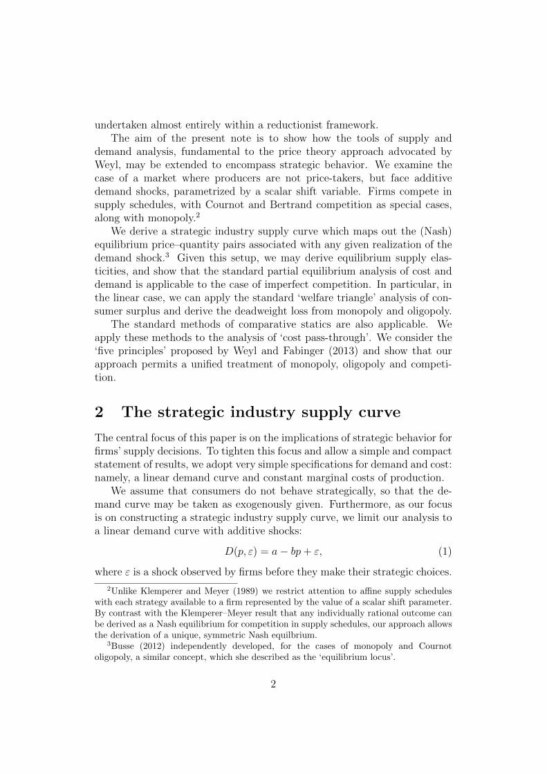
Abstract

In this paper we develop the concept of the strategic industry supply curve,representing the locus of Nash equilibrium outputs and prices arising fromadditive shocks to demand. We show that the standard analysis of partialequilibrium under perfect competition, including the graphical representa-tion of supply and demand due to Marshall, can be extended to encompassimperfectly competitive markets, including monopoly, Cournot and Bertrandoligopoly and competition in linear supply schedules. We then derive a uni-fied theory of cost pass-through and show that it satisfies the five principlesof incidence set out by Weyl and Fabinger (2013).

Keywords: industry supply, cost pass-through, oligopoly.JEL Code: D4, L1.

1 Introduction

Supply and demand curves, and associated concepts such as elasticities, havebeen central to partial equilibrium analysis since the 19th century. Supplyand demand analysis provides a simple and elegant way of modelling theeffects of shifts in consumer preferences, production costs and governmentinterventions such as taxes. The graphical representation of the derivation ofequilibrium prices and quantities as the intersection of demand and supplycurves is an instantly recognizable iconic representation of economics.

Although commonly attributed to Marshall (1890), supply and demandcurves were first presented by Cournot (1838), in the same volume that in-troduced his famous analysis of duopoly. The theoretical foundations of thedemand curve were developed shortly afterwards by Dupuit (1844). Despitethis overlap, Cournot and Dupuit worked in very different methodologicalframeworks, which Weyl (2017) distinguishes as ‘reductionist’ and ‘price the-ory’ respectively. Dupuit addressed institutional and historical factors as wellas the purely economic determinants of equilibrium that were the focus ofCournot’s analysis. Even more than Cournot’s duopoly analysis, these earlyinnovations were neglected, and the ideas were subsequently developed inde-pendently by a number of writers before being systematized by Marshall.1

Despite this early link with the theory of strategic behavior in imperfectlycompetitive markets, the supply–demand approach has been confined to thenon-strategic case of competitive markets, where firms and consumers maybe regarded as price takers. In this case, supply and demand quantities maybe represented as functions of prices, and the associated curves are the graphsof those functions.

In the polar case of monopoly, the standard graphical analysis begins withthe demand curve, which permits the derivation of the marginal revenuecurve. Profit-maximizing output is determined by the intersection of themarginal revenue and marginal cost curves, and the associated price maythen be read off the demand curve. In this standard analysis, there is noanalog to the supply curve.

For the more general case of oligopoly, supply–demand analysis is rarely,if ever, used. To the extent that a graphical representation of equilibriumdetermination is employed, the standard approach is to represent the prob-lem in terms of the reaction functions of the firms involved in a duopolymarket, and thereby illustrate the Nash equilibrium solution. That is, in theterminology of Weyl (2017), theoretical analysis of the oligopoly problem is

1Ekelund and Hebert (1999) provides a detailed discussion of Marshall’s predecessorsin the development of the supply–demand diagram.

1

undertaken almost entirely within a reductionist framework.The aim of the present note is to show how the tools of supply and

demand analysis, fundamental to the price theory approach advocated byWeyl, may be extended to encompass strategic behavior. We examine thecase of a market where producers are not price-takers, but face additivedemand shocks, parametrized by a scalar shift variable. Firms compete insupply schedules, with Cournot and Bertrand competition as special cases,along with monopoly.2

We derive a strategic industry supply curve which maps out the (Nash)equilibrium price–quantity pairs associated with any given realization of thedemand shock.3 Given this setup, we may derive equilibrium supply elas-ticities, and show that the standard partial equilibrium analysis of cost anddemand is applicable to the case of imperfect competition. In particular, inthe linear case, we can apply the standard ‘welfare triangle’ analysis of con-sumer surplus and derive the deadweight loss from monopoly and oligopoly.

The standard methods of comparative statics are also applicable. Weapply these methods to the analysis of ‘cost pass-through’. We consider the‘five principles’ proposed by Weyl and Fabinger (2013) and show that ourapproach permits a unified treatment of monopoly, oligopoly and competi-tion.

2 The strategic industry supply curve

The central focus of this paper is on the implications of strategic behavior forfirms’ supply decisions. To tighten this focus and allow a simple and compactstatement of results, we adopt very simple specifications for demand and cost:namely, a linear demand curve and constant marginal costs of production.

We assume that consumers do not behave strategically, so that the de-mand curve may be taken as exogenously given. Furthermore, as our focusis on constructing a strategic industry supply curve, we limit our analysis toa linear demand curve with additive shocks:

D(p, ε) = a− bp+ ε, (1)

where ε is a shock observed by firms before they make their strategic choices.

2Unlike Klemperer and Meyer (1989) we restrict attention to affine supply scheduleswith each strategy available to a firm represented by the value of a scalar shift parameter.By contrast with the Klemperer–Meyer result that any individually rational outcome canbe derived as a Nash equilibrium for competition in supply schedules, our approach allowsthe derivation of a unique, symmetric Nash equilbrium.

3Busse (2012) independently developed, for the cases of monopoly and Cournotoligopoly, a similar concept, which she described as the ‘equilibrium locus’.

2

It should be clear from our analysis below that the model can be extendedto more general demand functions, but at the expense of more complex anal-ysis to account for the curvature of the demand curve.4 As we will showbelow, for constant marginal costs, and competition in linear supply sched-ules, the strategic industry supply curve is also linear, further simplifying theanalysis.

In the case of competitive markets, graphical analysis using the supplycurve has the following desirable features. First, and most importantly, theequilibrium price and quantity are given by the intersection of the demandand supply curves. Second, we can undertake comparative static analysisboth with respect to shifts in the demand curve and with respect to costshocks. In the latter case, we can use the concept of ‘cost pass-through’ todescribe the equilibrium incidence of cost shocks.

In the general case of imperfect competition, the strategic choices of firmswill depend on the anticipated responses of other firms as well as on marketdemand. Hence, there is no uniquely defined relationship between marketprices and the quantity supplied by individual firms or by the industry as awhole.

Nevertheless, a form of the supply curve arises naturally when we con-sider the response to shifts in the demand curve, characterized by the shock(ε). For each value of ε, the (Nash) equilibrium strategic choices of firmsdetermine a market equilibrium, that is a price–quantity pair on the de-mand curve at which the market clears. The locus of such points will be aone-dimensional manifold, upward-sloping in price–quantity space, that is,a (strategic industry) supply curve. The analysis is particularly simple inthe case where the firms’ strategy spaces consist of a family of firm supplycurves, with a single strategic shift parameter, and particularly when boththe demand parameter and the strategic supply parameter represent additiveshifts.

We assume that firms n = 1, ..., N,N ≥ 1, choose strategies in linearsupply schedules

Sn = αn + βp (A2)

where αn is the strategic variable for firm n and β is an exogenously givenslope parameter, interpreted as representing the competitiveness of the mar-ket. Cournot competition is represented by β = 0. The opposite polar caseof Bertrand competition is approached as β →∞.

Firms seek to maximize profit

πn = (p− c)Sn4For a comprehensive treatment of the implications of non-linear demand see Weyl and

Fabinger (2013).

3

where c is the constant marginal cost of production.5

From the viewpoint of any given firm i, the strategic choices of the otherfirms n 6= i, along with the market demand curve and the realization of thedemand shock ε, determine the residual demand curve faced by that firm.Nash equilibrium requires that firm i chooses its optimal price–quantity pairfrom the residual demand curve, holding the strategic choices of the otherfirms, αn, n 6= i (and the exogenously given6 βn, n 6= i) constant.

It does not matter, however, whether firm i conceives of its own choiceas picking the strategic variable αi, the associated quantity or price, or someother variable such as the markup on marginal cost. All that matters isthat the decision variable should uniquely characterize the profit-maximizingprice–quantity pair on the residual demand curve for firm i.

The residual demand facing firm i, given the realized value of ε, is

qi (ε) = a− bp (ε)−∑n6=i

(αn + βp (ε)) + ε (2)

= a−∑n 6=i

αn − (b+ (N − 1) β) p (ε) + ε,

and firm i can be regarded as a monopolist facing this demand schedule.7

We can rearrange the expression above as:

p (ε) = θi (ε)− γiqi (ε)where

θi (ε) =a−

∑n 6=i αn + ε

b+ (N − 1) β(3)

γi =1

b+ (N − 1) β.

The same analysis is applicable to the case of monopoly, where N = 1, andthe expressions above become:

θ (ε) =a+ ε

b(4)

γ =1

b.

5The case of a general convex cost function is straightforward but complicates thestatement of the results. This case is addressed in an Appendix available, from the authors.

6In this paper, we have adopted the simplifying assumption that all firms have the sameβn. This assumption can be relaxed. The important point is that, from the perspective offirm i, it is the set of strategies available to other firms n 6= i that determine the residualdemand curve facing i. Whatever the strategy space for i, any point on the residual demandcurve may be selected as an equilibrium outcome.

7For the special case of monopoly, (2) is simply the demand curve.

4

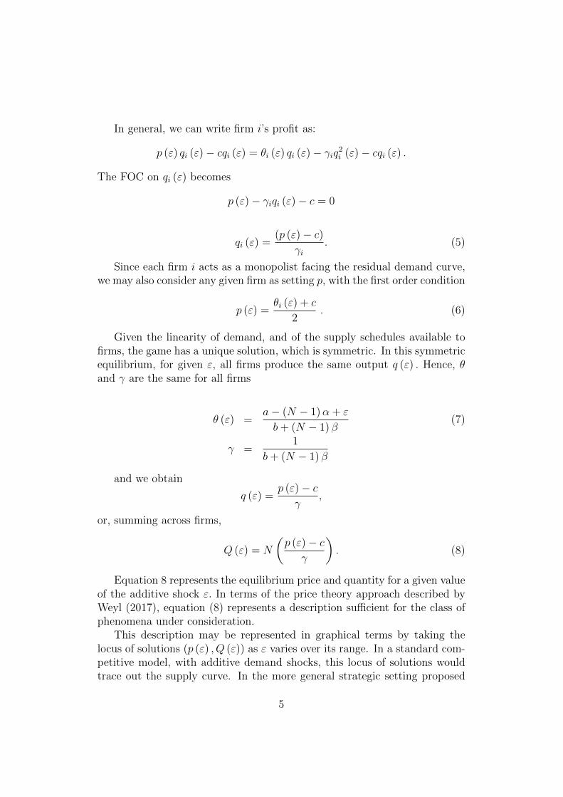
In general, we can write firm i’s profit as:

p (ε) qi (ε)− cqi (ε) = θi (ε) qi (ε)− γiq2i (ε)− cqi (ε) .

The FOC on qi (ε) becomes

p (ε)− γiqi (ε)− c = 0

qi (ε) =(p (ε)− c)

γi. (5)

Since each firm i acts as a monopolist facing the residual demand curve,we may also consider any given firm as setting p, with the first order condition

p (ε) =θi (ε) + c

2. (6)

Given the linearity of demand, and of the supply schedules available tofirms, the game has a unique solution, which is symmetric. In this symmetricequilibrium, for given ε, all firms produce the same output q (ε) . Hence, θand γ are the same for all firms

θ (ε) =a− (N − 1)α + ε

b+ (N − 1) β(7)

γ =1

b+ (N − 1) β

and we obtain

q (ε) =p (ε)− c

γ,

or, summing across firms,

Q (ε) = N

(p (ε)− c

γ

). (8)

Equation 8 represents the equilibrium price and quantity for a given valueof the additive shock ε. In terms of the price theory approach described byWeyl (2017), equation (8) represents a description sufficient for the class ofphenomena under consideration.

This description may be represented in graphical terms by taking thelocus of solutions (p (ε) , Q (ε)) as ε varies over its range. In a standard com-petitive model, with additive demand shocks, this locus of solutions wouldtrace out the supply curve. In the more general strategic setting proposed

5

here, we therefore refer to the locus of equilibrium solutions as the strategicindustry supply curve:

S (p) = N(p− c)γ

. (9)

By substituting the value of γ into (9), we obtain the following result:

Proposition 1 Given constant marginal costs and linear demand, the in-dustry supply curve is

S (p;N, β) = N (p− c) (b+ (N − 1) β) , (10)

which is linear with intercept c and slope 1N(b+(N−1)β)

in the p × S (p;N, β)axis.

For the monopoly case, the slope is 1b. For the symmetric oligopoly case,

the slope ranges between 1Nb

for Cournot (β = 0) and 0 in the limit as β →∞(Bertrand/perfect competition, where p→ c).

We also have:

Corollary 1 For the symmetric case with constant marginal costs, S ′ (p) =N (b+ (N − 1) β) >

∑βn = Nβ.

In particular, for the case of Cournot oligopoly, the strategic industrysupply curve is strictly upward sloping even though the firms’ equilibriumsupply schedules are all vertical. This reflects the fact that the strategicindustry supply curve is derived from a locus of equilibria, one for each valueof ε.

Menezes and Quiggin (2012) observe that an increase in the number ofcompetitors N will have similar effects on equilibrium market outcomes as anincrease in the competitiveness of the market (higher β). The concept of thestrategic industry supply curve enables us to sharpen this point. Consider asa benchmark the Cournot case, where S ′ (p) = Nb. Now, for any 2 ≤M < N,

let β (M) = (N−M)bM(M−1)

> 0. Then, for all p

S (p;N, 0) = S (p;M,β (M)) .

More generally, for any initial β and M < N, we can find β (M) suchthat, for all p,

S (p;N, β) = S (p;M,β (M)) .

6

Remark 1 The linear strategic industry supply curve (9) , obtained underconstant marginal cost, is equivalent to a competitive industry supply curvewith appropriately defined quadratic costs. For example, consider the costfunction c(Q) = γQ+ ξQ2, so that, under competition, p = γ + 2ξQ. This isequivalent to (10) with γ = c and ξ = 1

2N(b+(N−1)β).

We can now turn to the determination of the equilibrium. For given ε,(9) coincides with the equilibrium price and quantity and, therefore, it canbe used to determine the Nash equilibrium outcome:

p (ε) = c+a− bc+ ε(

Nγ

+ b) (11)

= c+γ (a− bc+ ε)

N + bγ(12)

Q (ε) =N

γ

a− bc+ ε(Nγ

+ b)

=N (a− bc+ ε)

N + bγ.

In the monopoly case, we obtain

pM (ε) = c+a− bc+ ε

2b

QM (ε) =a− bc+ ε

2.

For the symmetric oligopoly case, we denote the equilibrium price–quantitypair associated with slope parameter β and shock ε by

(pβ (ε) , Qβ (ε)

).

For Cournot, we set β = 0 in (7), to obtain γ = 1b

and

p0 (ε) = c+1

N + 1

a− bc+ ε

b

Q0 (ε) =N

N + 1(a− bc+ ε) ,

which reduces to the familiar p0 = 1N+1

, Q0 = NN+1

for zero cost, a = 1and ε = 0.

The Bertrand case is obtained by taking the limit of (7) as β → ∞,yielding γ → 0 and

p∞ (ε) = c

Q∞ (ε) = a− bc+ ε.

7

The elasticity of industry supply with respect to price is simply

εS =p

p− c.

This expression does not contain β explicitly, but the equilibrium price pdepends on β. As would be expected, εS approaches infinity for the Bertrandcase β → ∞. For Cournot, εS = 1 + Nbc

a−bp+ε . In particular, for the case of

zero costs, εS takes values in the range [1,∞).Our approach to constructing the strategic industry supply curve is illus-

trated, for the case of a symmetric Cournot duopoly with constant marginalcosts, in Figures 1 and 2 below.

Figure 1 shows how the Cournot equilibrium quantity was obtained forthree values of ε. For the case of linear demand (1), firm i’s reaction function,i = 1, 2, i 6= j, is given by:

qi =p− cγ

a− qj + ε− bc2

.

Figure 2 shows the derivation of the strategic industry supply curve, whichis obtained by tracing the equilibrium price–quantity supplied pairs as εvaries over its range.

In Figure 3 below, we show how the standard first-year supply–demandgraphical approach can be extended to the analysis of symmetric oligopolyand to the case of monopoly, drawn below for constant marginal cost c.

As it is clear from Figure 3, the strategic industry supply curve is anequilibrium concept in the sense that it is derived from the firms’ profitmaximization for each realization of demand.

3 Welfare

The construction of a strategic industry supply curve also allows us to un-dertake the standard graphical analysis of welfare using a supply–demanddiagram. This is illustrated in Figure 4 below for the case of linear demand(1) and constant marginal costs c. Figure 4 depicts consumer surplus (CS),producer surplus (PS), total surplus (TS) and deadweight loss (DWL) forgiven values of β and ε.

Under our construct, the direct demand (1) is parametrized by the real-ization of ε. Consumer surplus (CS) is given by:

CS (ε) =1

2(p0 (ε)− p)D(p, ε),

8

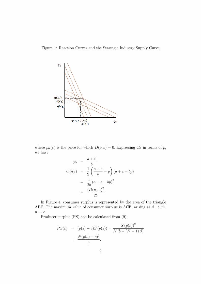
Figure 1: Reaction Curves and the Strategic Industry Supply Curve

where p0 (ε) is the price for which D(p, ε) = 0. Expressing CS in terms of p,we have

po =a+ ε

b

CS(ε) =1

2

(a+ ε

b− p)

(a+ ε− bp)

=1

2b(a+ ε− bp)2

=(D(p, ε))2

2b.

In Figure 4, consumer surplus is represented by the area of the triangleABF. The maximum value of consumer surplus is ACE, arising as β → ∞,p→ c.

Producer surplus (PS) can be calculated from (9):

PS(ε) = (p(ε)− c)S (p(ε)) =S (p(ε))2

N (b+ (N − 1) β)

=N(p(ε)− c)2

γ.

9

Figure 2: Strategic Industry Supply Curve (Cournot)

Note that producer surplus is not equal to the area of the triangle BEFbetween the price and the supply curve in Figure 4.8 Rather, in the case ofconstant marginal cost examined here, producer surplus for given ε is equalto the rectangle BDEF with height (p(ε)−c) and base Q(ε). That is, producersurplus in the case of a linear strategic supply curve and constant marginalis twice the surplus that arises in a competitive market with the same supplycurve resulting from increasing marginal cost.

Remark 2 As noted in remark 1, the strategic supply curve derived here isequivalent to a competitive supply curve with appropriately defined quadraticcosts. In this case, the producer surplus would be the triangle BEF while thecomplementary triangle BDE would represent costs incurred by producers.Thus, imperfect competition is analogous to a case where producers engage in‘cost-padding’ and recoup both the resulting producer surplus and the spuriouscosts.

8We are indebted to Glen Weyl for this observation.

10

Figure 3: Industry Strategic Supply Curve: Constant Marginal Cost

The total surplus (TS) associated with ε can be written as:

TS(ε) = CS(ε) + PS(ε) (13)

=Q(ε)

Nγ

2

+Q (ε)2

2b

where Q (ε) is the equilibrium output given by (11):

Q (ε) =(a− bc+ ε)N

N + bγ(14)

and is represented by the area ABDEF.The deadweight loss (DWL), relative to the Bertrand equilibrium p = c,

is:

DWL (ε) =1

2(p(ε)− c)(D(c, ε)−Q (ε)) (15)

=1

2

γQ(ε)

N(a− bc+ ε−Q (ε))

where D(c, ε) represents the quantity demanded, given ε, when p = c.

11

Figure 4: Welfare analysis with the strategic industry supply curve

Substituting (14) into (13) and (15) and simplifying yields:

TS(ε) =N (a− bc+ ε)2 (2b+Nγ)

2bγ (N + bγ)2 (16)

and

DWL (ε) =bγ2 (a− bc+ ε)2

2 (N + bγ)2 . (17)

As the calculations above hold for any value of ε, we can derive thefollowing result. The proof is omitted as it follows from inspection of (16)and (13):

Proposition 2 For the case of linear demand and constant marginal cost,consumer surplus and total surplus increase with β, while producer surplusand deadweight loss decrease with β.

12

4 Cost Pass-through

The problem of cost pass-through is a special case of the comparative staticsof Marshallian partial equilibrium analysis. The analysis begins with a marketequilibrium disturbed by a shock to suppliers’ input prices or technology,which may be represented as an increase of ∆c in unit costs. The problemis to determine the resulting change in the equilibrium price ∆p, and, moreparticularly, the ratio ρ = ∆p

∆c, which measures the proportion of the cost

increase passed through to consumers. Although input prices and technologyare subject to constant change, the term ‘pass-through’ is most commonlyused in contexts where the change in equilibrium prices is seen to be of policyconcern.

The problem of cost pass-through was recently examined by Weyl andFabinger (2013), who draw on a long tradition of work on tax incidence, goingback to Dupuit (1844), Jenkin (1871-72) and Marshall (1890). Like Weyl andFabinger, we extend the standard analysis of incidence under competition tothe case of imperfectly competitive markets. Although our representation ofthe problem is different, it is equivalent to that of Weyl and Fabinger in somecases, most notably that of a monopolist facing linear demand. Our resultsfor that case coincide with theirs, as we shall show.

For the case of symmetric oligopoly, there are subtle differences. Thesearise from the fact that Weyl and Fabinger focus on a conjectural variationsmodel derived from the work of Bresnahan (1981). By contrast, our analysisbegins with a Nash equilibrium in affine supply schedules, as derived above.We explore some of the similarities and distinctions below.

The following proposition can be derived directly from (11):

Proposition 3 Cost pass-through for symmetric oligopoly with constant marginalcost is given by:

ρ =Nb+N (N − 1) β

(N + 1) b+N (N − 1) β. (18)

From (18), we can recover the standard pass-through expression for Cournotmodels with linear demand and constant marginal cost (ρ = N

N+1). For

Bertrand (when β →∞) cost pass-through is equal to 1, as for perfect com-petition. As observed above, an increase in the number of competitors N hasthe same effect as an appropriately chosen increase in β. In particular, forany fixed β, as N → ∞, ρ → 1. The minimum value of ρ is ρ = 1

2, attained

in the monopoly case N = 1.The Bertrand and Cournot examples are shown in Figure 5 below.

13

Figure 5: Cost Pass Through for Cournot and Bertrand

The next proposition relates (18) to the relevant elasticities, namely thatof demand and of the strategic industry supply curve, extending the standardanalysis of cost pass-through to cover monopoly and (symmetric) oligopoly.

Proposition 4 Cost pass-through is given by

ρ =εS

εD + εS,

where εD denotes the price elasticity of demand and εS the price elasticity ofthe strategic industry supply curve.

Proof. The expression for εD can be derived as follows

εD = −∂D(p, ε)

∂p

p

D(p, ε)=

bp

a+ ε− bp.

Substituting the expression for (11) yields:

εD =b [c [(N + 1) b+N (N − 1) β] + a− bc+ ε]

(a− bc+ ε) [(N + 1) b+N (N − 1) β − bc].

14

Similarly, replacing (11) into the expression for εS = pp−c yields:

=c [(N + 1) b+N (N − 1) β] + a− bc+ ε

a− bc+ ε.

It follows, by simple algebra, that

εSεD + εS

= 1− b

[(N + 1) b+N (N − 1) β]= ρ.

For the special case of monopoly, we have ρ = 1/2. For Cournot, ρ = NN+1

.For Bertrand, ρ = 1.

4.1 Incidence

Now consider the case when a cost increase arises from the imposition of atax. In this case, we are interested in the tax burden, that is, the ratio ofthe loss in producer and consumer surplus to the revenue raised by the tax.

Consider the case when a tax t is imposed. In the linear case consid-ered here, local and global analysis will coincide. However, for notationalconvenience we will focus on derivatives evaluated at t = 0.

We have, for producer surplus,

∂PS(ε)

∂t=

2N

γ(p(ε)− c)∂(p(ε)− c)

∂t

= (ρ− 1)2N

γ(p(ε)− c)

= (ρ− 1)Q (ε)

= 2 (ρ− 1)∂R

∂t

where R = tQ (ε) is tax revenue.For consumer surplus,

CS =1

2b(a+ ε− bp)2 .

So, in equilibrium.

∂CS

∂t= − (a+ ε− bp) ∂p

∂t= −ρQ

= −ρ∂R∂t

=ρ

2 (1− ρ)

∂PS(ε)

∂t.

15

The total burden of the tax is given by∣∣∣∣∂PS(ε)

∂t+∂CS

∂t

∣∣∣∣ = (2− ρ)∂R

∂t

≥ ∂R

∂t,

where equality holds only for the Bertrand case ρ = 1.For the Bertrand case, we have

∂PS(ε)

∂t= 2 (ρ− 1)

∂R

∂t= 0

∂CS(ε)

∂t= −∂R

∂t

That is. the burden of a small tax is entirely borne by consumers, andthere is no deadweight loss. For monopoly, ρ = 1

2, and we have

∂PS(ε)

∂t= −∂R

∂t∂CS(ε)

∂t= −1

2

∂R

∂t.

Thus, we obtain the well known result that the full tax revenue is paidby the monopolist, and an additional burden is borne by consumers. In thelinear case considered here, this additional burden is equal to half of therevenue raised by the tax.

For Cournot ρ = NN+1

, we have

∂PS(ε)

∂t= − 2

N + 1

∂R

∂t∂CS(ε)

∂t= − N

N + 1

∂R

∂t∣∣∣∣∂PS(ε)

∂t+∂CS(ε)

∂t

∣∣∣∣ =N + 2

N + 1

∂R

∂t

I =N

2

where I (incidence) is the ratio of the burden borne by consumers to theburden borne by producers.

16

For the general oligopoly case, with β <∞ and N > 1, we have

∂CS(ε)

∂t= − Nb+N (N − 1) β

(N + 1) b+N (N − 1) β

∂R

∂t

∂CS(ε)

∂t= − 2b

(N + 1) b+N (N − 1) β

∂R

∂t∣∣∣∣∂PS(ε)

∂t+∂CS(ε)

∂t

∣∣∣∣ =(N + 2) b+N (N − 1) β

(N + 1) b+N (N − 1) β

∂R

∂t

I =Nb+N (N − 1) β

2b.

Once again, the total burden exceeds revenue and is shared between pro-ducers and consumers. Producers bear less than the full burden of the tax.

To sum up, the concept of the strategic industry supply curve yields aunified analysis of cost pass-through, encompassing the cases of monopoly,symmetric oligopoly and competition (interpreted either as oligopoly withBertrand competition or as competition between large numbers of firms).

5 The five principles

Weyl and Fabinger (2013) analyze the problem of cost pass-through, drawingon the literature on tax incidence. Their analysis is organized around fiveprinciples, drawing on the analysis of tax incidence under perfect competi-tion. These principles are extended, with appropriate modifications, to thecases of monopoly and oligopoly.

To analyze pass-through, Weyl and Fabinger introduce the elasticity ofthe inverse marginal cost curve, and of the inverse marginal surplus curve.Weyl and Fabinger denote the elasticity of the inverse marginal cost curveby εs, but we have used this notation for the elasticity of the industry supplycurve. We will therefore denote the elasticity of the inverse marginal costcurve by εc. Because we focus on linear demand, the elasticity of the in-verse marginal surplus curve is identically equal to 1, and we will make thissubstitution throughout in stating the Weyl–Fabinger principles.

In the case of symmetric oligopoly with a homogenous product, the com-petitiveness of the market is represented by a parameter R, which variesbetween 0 (for Cournot) and −1 (for Bertrand). Weyl and Fabinger usethe derived variable θ = 1+R

N, which varies between 0 (Bertrand) and 1

N

(Cournot). A straightforward manipulation shows that, translating to theterms of our model, we have θ = 1

N+Nβ(N−1). Thus, our model provides an

explicit game-theoretic foundation for the derivation of the parameters Rand θ.

17

The idea of the strategic industry supply curve allows for a more uni-fied treatment of the Weyl–Fabinger principles, with a single statement ofthe principles applicable to competition, monopoly and oligopoly. As in theargument above, we will confine attention to the case of linear demand andconstant marginal costs, so that the only variation arises from the competi-tiveness or otherwise of the market structure.

We now consider the Weyl–Fabinger principles in turn:Principle of incidence 1 (Economic versus physical incidence)The physical incidence of taxes is neutral in the sense that a tax levied on

consumers, or a unit parallel downward shift in consumer inverse demand,causes nominal prices to consumers to fall by 1− ρ.

This principle of neutrality is fundamental. The same principle underliesthe crucial observation that from the viewpoint of any individual producer,a shock to residual demand is identical whether it arises from a shock tomarket demand or from the (equilibrium) supply of other producers. Weyland Fabinger (2013) attribute this insight to Jeremy Bulow.

Principle of incidence 2 (Split of tax burden)(i) Under competition, the total burden of the infinitesimal tax beginning

from zero tax is equal to the tax revenue and is shared between consumersand producers.

(ii) Under monopoly, the total burden of the tax is more than fully sharedby consumers and producers. While the monopolist fully pays the tax out ofher welfare, consumers also bear an excess burden.

(iii) Under homogenous products oligopoly, the total burden of the taxis more than fully shared by consumers and producers. Producers bear lessthan the full burden of the tax.

As shown above, Principle 2 is satisfied by our model.Principle of incidence 3 (Local incidence formula)

The ratio of the tax borne by consumers to that borne by producers, theincidence, I, equals:

(i) ρ1−ρ in the case of perfect competition;

(ii) ρ in the case of monopoly; and(iii) ρ

1−(1−θ)ρ in the case of oligopoly.Our results coincide with those of Weyl and Fabinger in all cases.Principle of incidence 4 (Pass– through)

The pass-through rate is:(i) ρ = 1

1+εD/εCin the case of perfect competition;

(ii) ρ = 12+(εD−1)/εC

in the case of monopoly; and

(iii) ρ = 11+θ+ θ

εθ+(εD−θ)/εC

in the case of oligopoly.

18

For the special case of constant marginal costs, εC is infinite, so we obtainρ = 1 for competition and ρ = 1

2for monopoly. For the case of linear supply

schedules, β and therefore also θ are constant. Hence εθ is also infinite,so ρ = 1

1+θ. Substituting θ = 1

N+Nβ(N−1)into this expression, we obtain

ρ = N+[(N+1)+N(N−1)β][(N+1)+N(N−1)β]

, which coincides with our result for the case b = 1.Finally, we havePrinciple of incidence 5 (Global incidence)Weyl and Fabinger derive global incidence as a weighted average of the

pass-through rate which is, in general, variable. For the case of linear de-mand, considered here, the pass-through rate is constant, and therefore globalincidence is the same as local incidence. The extension of our analysis to thecase of non-linear demand can be undertaken using the tools provided byWeyl and Fabinger.

6 Concluding comments

We have shown that, using the concept of the strategic industry supply curve,the standard analysis of partial equilibrium under perfect competition, in-cluding the graphical representation of supply and demand due to Marshall,can be extended to encompass imperfectly competitive markets. The classof market structures encompasses monopoly and competition, as well as anentire class of oligopoly models represented by competition in linear supplyschedules, with Cournot and Bertrand as polar cases. For the oligopoly case,the results show the interaction between the number of firms N and thecompetitiveness of the market structure, characterized by the parameter β.

Furthermore, this representation of supply allows for a unified treatmentof comparative static problems such as cost pass-through, which have previ-ously required separate treatments for competition, monopoly and oligopoly.In particular, we provide both a game-theoretic foundation for and a simplederivation of the Weyl–Fabinger principles of incidence. The tools used herecould be applied to a wide range of problems, such as the analysis of mergers.Similarly, we can extend the diagrammatic tools of welfare analysis, such asthe representation of deadweight losses as welfare triangles.

The analysis here has focused on the case of linear demand and constantmarginal cost, to allow for a simple statement of results that illuminates thecrucial aspects of the problem, and to permit a simple graphical representa-tion. But the concept of the strategic industry supply curve is valid undermore general conditions.

We have not addressed issues of estimation. However, by observing mar-ket outcomes in the presence of demand shocks, it should be possible to use

19

standard techniques to estimate the strategic industry supply curve. Com-bined with information about technology and input costs, the slope of theestimated industry supply curve would provide information about the com-petitiveness of the market, measured by the slope of the supply curves avail-able as strategies to individual firms.

References

[1] Bresnahan, T. (1981), ‘Duopoly models with consistent conjectures’,American Economic Review, 71(5), 934–945.

[2] Busse, M. (2012), ‘When supply and demand just won’t do: using theequilibrium locus to think about comparative statics’, mimeo, North-western University.

[3] Cournot, A. (1838) Recherches Sur Les Principes Mathematiques De LaTheorie Des Richesses, Librairie des Sciences Politiques et Sociales. M.Riviere et Cie., Paris.

[4] Dupuit, A. J. E. J. (1844), De la mesure de l’utilite´ des travaux publics.Paris.

[5] Ekelund, R.B. and Hebert, R.F. (1999) Secret Origins of Modern Mi-croeconomics: Dupuit and the Engineers, University of Chicago Press,Chicago.

[6] Jenkin, H. C. F. (1871–72), ‘On the Principles Which Regulate the In-cidence of Taxes’, Proc. Royal Soc. Edinburgh, 7, 618–31.

[7] Klemperer, P.D. and Meyer, M.A. (1989), ‘Supply function equilibria inoligopoly under uncertainty’, Econometrica, 57(6), 1243–77.

[8] Marshall, A. (1890), Principles of Economics. New York: Macmillan.

[9] Menezes, F. and Quiggin, J. (2012), ‘More competitors or more com-petition? Market concentration and the intensity of competition’, Eco-nomics Letters, 117(3), 712–714.

[10] Weyl, E. G. and Fabinger, M. (2013), ‘Pass-Through as an EconomicTool: Principles of Incidence under Imperfect Competition,’ Journal ofPolitical Economy, 123(3), 528-583.

[11] Weyl (2017), Price Theory, working paper, Microsoft Research New YorkCity.

20