The stiffness of short and randomly distributed fiber …...The stiffness of short and randomly distributed fiber composites E. SIDERIDIS, J. VENETIS, V. KYTOPOULOS School of Applied

The stiffness of short and randomly distributed fiber composites

E. SIDERIDIS, J. VENETIS, V. KYTOPOULOS School of Applied Mathematics And Physical Sciences, Section Of Mechanics

National Technical University of Athens 5 Heroes Of Polytechnion Avenue, Gr – 15773 Athens

GREECE Telephone: +302107721251

Fax: +302107721302 Email: [email protected], [email protected], [email protected]

Abstract: In this work, analytical calculations are described to estimate the elastic moduli of polymer composite materials consisting of short fibers, by extending and generalizing a reliable model. The fibers may have a finite length and an orientation characterized as random. An effort was made to complete and improve a previous procedure concerning transversely isotropic composites. To this end, a cylinder model with a short fiber in the centre of the matrix is considered. The elastic moduli were expressed in terms of the fiber content and fiber length. The obtained representations were used to evaluate the moduli of a randomly oriented short fiber composite. A comparison was made with theoretical values derived from two other authors who established trustworthy and accurate models. Finally, our theoretical values were also compared with obtained experimental results. Keywords: Fiber composite materials, short fibers, unit cell, elastic constants, model of equivalent fiber, fiber contiguity 1 Introduction It is well known that from the commercial standpoint the composite materials are made from matrices of epoxy, unsaturated polyester and in addition of some other thermosets and a f ew thermoplastics. The reinforcements are glass, graphite, aramid, thermoplastic fibers, metal and ceramic. The reinforcement may be continuous, woven, or chopped fiber and a typical commercial composite contains from 20% to 50% by weight glass or other reinforcement. The percentage of reinforcement in advanced composites can be as high as 70%; these materials usually use epoxy as the matrix material, and graphite is the most common reinforcement. Glass fibers are usually used for low cost and wherever high stiffness is not necessary. The purpose of adding reinforcements to polymers is usually to enhance mechanical properties. One of the most useful forms of composites for the construction of high – performance structural elements, is the type of panels made from aligned fibers containing polymerized matrix. They can also be made with woven fibers or randomly oriented chopped fibers; these have inferior stiffness and cannot have such high fiber materials. In order to perform stress and stiffness analyses of the chopped – fiber resin composites, it is essential that the elastic properties be known.

In reality, these materials are anisotropic and heterogeneous. Evidently, their properties depend on the elastic properties and volume fractions of the constituent materials, the fiber length or aspect ratio, the degree of the alignment, the adhesion between fibers and matrix and finally they are affected by the fabrication techniques. Nevertheless, one should primarily elucidate that chopped fibers, flakes, particles, and similar discontinuous reinforcements may enhance short – term mechanical properties, but these types of reinforcements are usually not as ef fective as continuous reinforcements in increasing creep strength and similar long – term strength characteristics, since continuous reinforcements serve to distribute applied loads and strain throughout the entire structure. If the fibers are randomly distributed with respect to orientation and position, then samples of material which contain statistically significant numbers of fibers seem to be isotropic. If several such samples are compared to one another, the material can be considered as h omogeneous. I f the fibers have a specific orientation, then the composite will be anisotropic. Besides, in case the statistical distribution of fillers’ orientation varies with position, then the composite becomes inhomogeneous even if the fiber density is uniform. Mostly, theoretical studies for the stiffness and strength of such materials have been concerned

WSEAS TRANSACTIONS on APPLIED and THEORETICAL MECHANICS E. Sideridis, J. Venetis, V. Kytopoulos

E-ISSN: 2224-3429 53 Volume 13, 2018

with the aligned case, or with the situation of cross – ply laminates of continuous unidirectional fibers. The application of materials reinforced with short randomly – oriented f ibers is not relatively new. For some reasons, the fibers may be arranged such that they have partially aligned whereby they are constrained to lie in a plane but are otherwise randomly oriented. Generally, the elastic moduli of a chopped – fiber composite can be derived from those of a unidirectional discontinuous fiber composite through a normalized integration process. There have been several previous studies of the random fiber case. T he first such study was apparently that due to Cox [1] who studied the stiffness of cellulose fiber materials by assuming that the external load is carried entirely by the fibers. The result was the Cox formula i.e.

33ff

D

UEE =

where fE is the fiber modulus and fU the its volume fraction. The corresponding result for the two dimensional case was found to be

32

ffD

UEE =

The first consideration of fiber – matrix effects was provided by Tsai and Pagano [2], in the context of laminated plates. Nielson and Chen [3] used computational techniques to predict the modulus of the composite. Further work along the lines using the “Laminate analogy” was given by Halpin, Jerina and Whitney [4]. Lees [5], in order to explain his experimental data concerning the longitudinal modulus derived a formula for the elastic modulus of short fiber composites assuming that the fiber and the matrix have different longitudinal strain under axial loading. One of the most important theories developed is that of Christensen and Waals [6], who provided a method for determining random orientation properties using a geometric averaging method. Later, Christensen [7], thought that there is a need to obtain analytical forms which directly admit physical interpretation. Assuming that the fiber phase is much stiffer than the matrix one he simplified the expressions based on the classical results of Hill [8,9] and Hashin [10,11] on unidirectional transversely isotropic composites which after a normalized integration process yield the elastic moduli of a randomly oriented fiber composite. The results for the three and two

dimensional case respectively are represented as follows

mff

ff

fD E

UUU

UE

E

++

−+=

641

11

6

2

3 ;

mfmff

fmffm

ff

fD E

UEUEUEUE

EU

UE

E)1()1()1()1(

2719

31

32 ++−−++

+−

+=

where mE is the matrix modulus The procedure presented in Ref. [6] was used by Eisenberg [12] in order to derive expressions which take into consideration the fabrication induced anisotropy of chopped – fiber resin composites. Except for the theory of Halpin and Pagano [2, 4], the above discussed theories do not consider the influence of fiber length or aspect ratio and therefore they are applicable for continuous fiber composites. There are several theoretical formulae appearing in the literature to study the elastic moduli of unidirectional short fiber composites. Ogorkievicz and Weidman [13] idealized the composite consisting of a polymeric matrix containing unidirectionally aligned discontinuous glass fibers into a prism of the polymeric material and within it, a prism of glass. The volume of the glass prism, expressed as a fraction of the volume of the larger prism is equal to the volume fraction of the glass fibers and its proportions are fixed by the aspect ratio of the fibers. Some assumptions and a strength of materials approach led to Eq. (4) for the modulus. A theory to enable prediction of moduli from basic matrix and fiber properties is due to Krenchel [14] who considered the composite to comprise a number of plies of uniaxially aligned fibers with the fibers of each ply being aligned in a different direction. The fiber – ply contributions are summed together with a contribution due to the matrix to give the continuous fibers length correction factors have been proposed to account for the reduction in composite stiffness that occurs with fibers of finite length. The factor proposed by Cox [1] is presented in the previous equations in a form which takes into account the wide distribution of fiber lengths. Halpin et al [15] adopted a more rigorous approach towards the prediction of the anisotropy of stiffness due to fiber orientation. They considered the composite to consist of a number of plies, each one containing matrix and uniaxially aligned fibers, again with the fibers of each ply to be aligned in a different direction. The moduli of each ply can be estimated. The simple relationships in these

WSEAS TRANSACTIONS on APPLIED and THEORETICAL MECHANICS E. Sideridis, J. Venetis, V. Kytopoulos

E-ISSN: 2224-3429 54 Volume 13, 2018

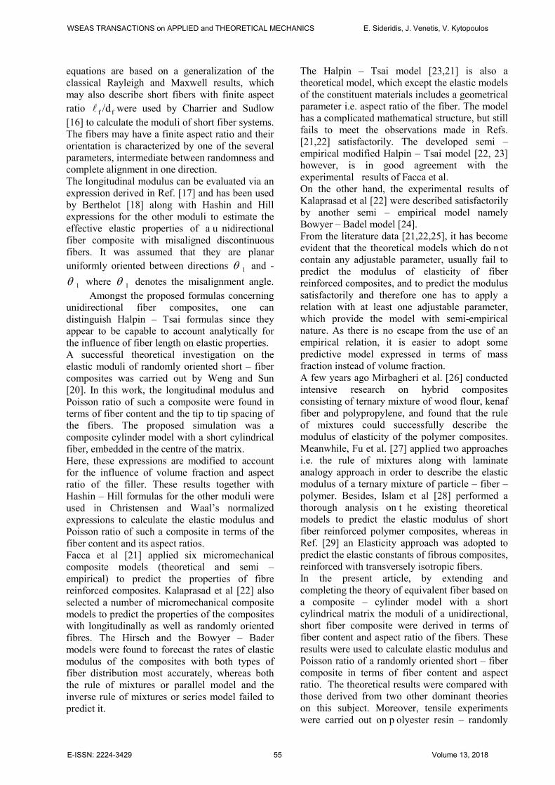
equations are based on a generalization of the classical Rayleigh and Maxwell results, which may also describe short fibers with finite aspect ratio ff /d were used by Charrier and Sudlow [16] to calculate the moduli of short fiber systems. The fibers may have a finite aspect ratio and their orientation is characterized by one of the several parameters, intermediate between randomness and complete alignment in one direction. The longitudinal modulus can be evaluated via an expression derived in Ref. [17] and has been used by Berthelot [18] along with Hashin and Hill expressions for the other moduli to estimate the effective elastic properties of a u nidirectional fiber composite with misaligned discontinuous fibers. It was assumed that they are planar uniformly oriented between directions 1θ and -

1θ where 1θ denotes the misalignment angle. Amongst the proposed formulas concerning unidirectional fiber composites, one can distinguish Halpin – Tsai formulas since they appear to be capable to account analytically for the influence of fiber length on elastic properties. A successful theoretical investigation on the elastic moduli of randomly oriented short – fiber composites was carried out by Weng and Sun [20]. In this work, the longitudinal modulus and Poisson ratio of such a composite were found in terms of fiber content and the tip to tip spacing of the fibers. The proposed simulation was a composite cylinder model with a short cylindrical fiber, embedded in the centre of the matrix. Here, these expressions are modified to account for the influence of volume fraction and aspect ratio of the filler. These results together with Hashin – Hill formulas for the other moduli were used in Christensen and Waal’s normalized expressions to calculate the elastic modulus and Poisson ratio of such a composite in terms of the fiber content and its aspect ratios. Facca et al [21] applied six micromechanical composite models (theoretical and semi – empirical) to predict the properties of fibre reinforced composites. Kalaprasad et al [22] also selected a number of micromechanical composite models to predict the properties of the composites with longitudinally as well as randomly oriented fibres. The Hirsch and the Bowyer – Bader models were found to forecast the rates of elastic modulus of the composites with both types of fiber distribution most accurately, whereas both the rule of mixtures or parallel model and the inverse rule of mixtures or series model failed to predict it.

The Halpin – Tsai model [23,21] is also a theoretical model, which except the elastic models of the constituent materials includes a geometrical parameter i.e. aspect ratio of the fiber. The model has a complicated mathematical structure, but still fails to meet the observations made in Refs. [21,22] satisfactorily. The developed semi – empirical modified Halpin – Tsai model [22, 23] however, is in good agreement with the experimental results of Facca et al. On the other hand, the experimental results of Kalaprasad et al [22] were described satisfactorily by another semi – empirical model namely Bowyer – Badel model [24]. From the literature data [21,22,25], it has become evident that the theoretical models which do n ot contain any adjustable parameter, usually fail to predict the modulus of elasticity of fiber reinforced composites, and to predict the modulus satisfactorily and therefore one has to apply a relation with at least one adjustable parameter, which provide the model with semi-empirical nature. As there is no escape from the use of an empirical relation, it is easier to adopt some predictive model expressed in terms of mass fraction instead of volume fraction. A few years ago Mirbagheri et al. [26] conducted intensive research on hybrid composites consisting of ternary mixture of wood flour, kenaf fiber and polypropylene, and found that the rule of mixtures could successfully describe the modulus of elasticity of the polymer composites. Meanwhile, Fu et al. [27] applied two approaches i.e. the rule of mixtures along with laminate analogy approach in order to describe the elastic modulus of a ternary mixture of particle – fiber – polymer. Besides, Islam et al [28] performed a thorough analysis on t he existing theoretical models to predict the elastic modulus of short fiber reinforced polymer composites, whereas in Ref. [29] an Elasticity approach was adopted to predict the elastic constants of fibrous composites, reinforced with transversely isotropic fibers. In the present article, by extending and completing the theory of equivalent fiber based on a composite – cylinder model with a short cylindrical matrix the moduli of a unidirectional, short fiber composite were derived in terms of fiber content and aspect ratio of the fibers. These results were used to calculate elastic modulus and Poisson ratio of a randomly oriented short – fiber composite in terms of fiber content and aspect ratio. The theoretical results were compared with those derived from two other dominant theories on this subject. Moreover, tensile experiments were carried out on p olyester resin – randomly

WSEAS TRANSACTIONS on APPLIED and THEORETICAL MECHANICS E. Sideridis, J. Venetis, V. Kytopoulos

E-ISSN: 2224-3429 55 Volume 13, 2018

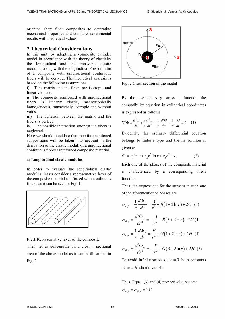
oriented short fiber composites to determine mechanical properties and compare experimental results with theoretical values. 2 Theoretical Considerations In this unit, by adopting a composite cylinder model in accordance with the theory of elasticity the longitudinal and the transverse elastic modulus, along with the longitudinal Poisson ratio of a composite with unidirectional continuous fibers will be derived. The theoretical analysis is based on the following assumptions: i) T he matrix and the fibers are isotropic and linearly elastic. ii) The composite reinforced with unidirectional fibers is linearly elastic, macroscopically homogeneous, transversely isotropic and without voids. iii) The adhesion between the matrix and the fibers is perfect. iv) The possible interaction amongst the fibers is neglected. Here we should elucidate that the aforementioned suppositions will be taken into account in the derivation of the elastic moduli of a unidirectional continuous fibrous reinforced composite material. a) Longitudinal elastic modulus In order to evaluate the longitudinal elastic modulus, let us consider a representative layer of the composite material reinforced with continuous fibers, as it can be seen in Fig. 1.

Fig.1 Representative layer of the composite

Then, let us concentrate on a cross – sectional

area of the above model as it can be illustrated in

Fig. 2.

Fig. 2 Cross section of the model

By the use of Airy stress – function the

compatibility equation in cylindrical coordinates

is expressed as follows 4 3 2

24 3 2 2 3

2 1 1 0d d d ddr r dr r dr r drΦ Φ Φ Φ

∇ Φ = + − + = (1)

Evidently, this ordinary differential equation

belongs to Euler’s type and the its solution is

given as 2 2

1 2 3 4ln lnc r c r r c r cΦ = + + + (2)

Each one of the phases of the composite material

is characterized by a corresponding stress

function.

Thus, the expressions for the stresses in each one

of the aforementioned phases are

( ), 2

1 1 2ln 2fr f

d A B r Cr dr r

σΦ

= = + + + (3)

( )2

, 2 2 3 2 ln 2ff

d A B r Cdr rθσΦ

= = − + + + (4)

( ), 2

1 1 2ln 2mr m

d F G r Hr dr r

σ Φ= = + + + (5)

( )2

, 2 2 3 2 ln 2mm

d F G r Hdr rθσΦ

= = − + + + (6)

To avoid infinite stresses at 0r = both constants

A και B should vanish.

Thus, Eqns. (3) and (4) respectively, become

, , 2r f f Cθσ σ= =

WSEAS TRANSACTIONS on APPLIED and THEORETICAL MECHANICS E. Sideridis, J. Venetis, V. Kytopoulos

E-ISSN: 2224-3429 56 Volume 13, 2018

For the matrix material, it can be shown that

0G = and therefore

, 2 2r mF Hr

σ = + and , 2 2mF Hrθσ = − +

Next, let us apply a tensile stress cσ , which is

exerted at the direction of z axis.

The equilibrium of forces at this direction yields

the following relationship

ccmmff AAA ⋅=⋅+⋅ σσσ (7)

with

, ,,z f f z m mσ σ σ σ= =

where

cmf AAA ,, is the area of the fiber, matrix, and

composite respectively.

Now, if one puts 1f sσ = , 2m sσ = , c sσ = and

divide by the term cF the above relationship

becomes

sUsUs mf =⋅+⋅ 21 (8)

where

2

2

m

ff r

rU = and 2

22

m

fmm r

rrU

−= are the fiber and

matrix content respectively

Evidently, 1=+ mf UU

Moreover, from the stress – strain relationships

we deduce that

( )[ ]1, 221 sCUCE f

ffr +−=ε (9)

( ) ( )

−−−+= 22, 1211 sUUHUrF

E mmmm

mrε (10)

( )[ ]1, 221 sCUCE f

ff +−=θε (11)

( ) ( )

−−−+= 22, 1211 sUUHUrF

E mmmm

mθε (12)

[ ]CUsE f

ffz 41

1, −=ε (13)

[ ]HUsE m

mmz 41

2, −=ε (14)

where Ef and Em are the elastic moduli of fiber

and matrix respectively

Meanwhile, the radial displacements are given as

, ,r f fu r θε= and , ,r m mu r θε=

In continuing, the boundary conditions are

formulated as follows

At fr r=

, , 22 2r f r mf

FC Hr

σ σ= → = + (15)

At mr r=

, 20 2 0r mf

F Hr

σ = → + = (16)

At fr r=

⇒= frfr uu ,,

( )[ ] ( ) ( )

−−++−=−− 221 12112 sUUHU

rFEsUUCE mmm

ffffm

(17)

Since the axial strains in matrix and fiber

coincide, it implies that

)4()4( 21 mffm HUsECUsE −=− (18)

The solution of the system of eqns. (17) and (18)

for the terms 1s and 2s respectively yields

fmmff

mffmf UUEUE

UHEUCEsEs

+

−+=

)(41

(19)

fmmff

mffmf UUEUE

UHEUCEsEs

+

−−=

)(42 (20)

A substitution of the above data back into Eqn.

(18) gives

fmmffmmmmmffffmmfff EUEUEvrC

FEUvEUvEvUEUEvf

))(1(2

)())(1( 2 ++−=+−+−

[ ]C

sWEUvEUvEvUEUEvCH

fmfmfmfmmmffm 2)())(1( ++−+−+ (21)

WSEAS TRANSACTIONS on APPLIED and THEORETICAL MECHANICS E. Sideridis, J. Venetis, V. Kytopoulos

E-ISSN: 2224-3429 57 Volume 13, 2018

where νf and νm are the Poisson ratios of fiber and

matrix respectively

From the solution of the system of eqns. (15),

(16) and (21) one estimates the rates of the

constants F , H , C as follows

sUKPLK

WrF

f

f

)()(

2

−++= (22)

sUKPLK

WUH

f

f

)()(2

−++= (23)

sUKPLK

UWC

f

f

)()()1(

2−++

−= (24)

with

fmmffmffmmfff EvUEvUEvUEUEvK ))(2))(1(( +−+−= (25)

fmmffm EUEUEvL ))(1( ++= (26)

ffmmmffmmmffm EvUEvUEvUEUEvP ))(2))(1(( +−+−= (27)

( )f m f mW v v E E= − (28)

A combination between the system of eqns. (25)

to (28) and the system of eqns. (19) and (20)

results in the following explicit expressions for

the quantities 1s and 2s respectively

( )( ) ⇒

−+++

+−⋅+

+= s

UKPLKUEUEvUEvEUUW

UEUEE

sfmmff

mfffmfm

mmff

f

)()()()1(2

1

ss ⋅=η1 (29)

and

( )( )⇒−+++

+−⋅−

+=

fmmff

mfffmff

mmff

m

UKPLKUEUEvUEvEUUW

UEUEE

ss

)()()()1(22

ss ⋅= ξ2 (30)

The longitudinal modulus EL of the composite can

be estimated by the equalization of the overall

deformation energy with the sum of

corresponding ones for the constituent materials.

Hence we can write out

( )∫∫ +++=fc V

ffzfzfffrfrV

cL

dVdVEs

,,,,,,

2

21

21

εσεσεσ θθ

( )∫ ++mV

mmzmzmmmrmr dV,,,,,,21 εσεσεσ θθ (31)

Since we have initially proposed a modified

version of Hashin cylinder model, the last

relationship can be equivalently recasted as

follows

( )

( )

2

, , , , , ,0

, , , , , ,

1 12 22 2

1 22

f

c

m

f

r

r f r f f f z f z fLV

r

r m r m m m z m z mr

s rhdr rhdrE

rhdr

θ θ

θ θ

π σ ε σ ε σ ε π

σ ε σ ε σ ε π

= + +

+ + +

∫ ∫

∫

(32)

Finally, by substituting the above expressions for

both stresses and strains back into eqn. (32) one

finds

( )

( )

2 2

2 2 2

1 1 8 (1 ) 8

1 2 8 (1 ) 8 (1 )

f f fL f

f m m fm

C v Cv UE E

F U H v Hv UE

η η

ξ ξ

= − − +

+ + − − + −

(33)

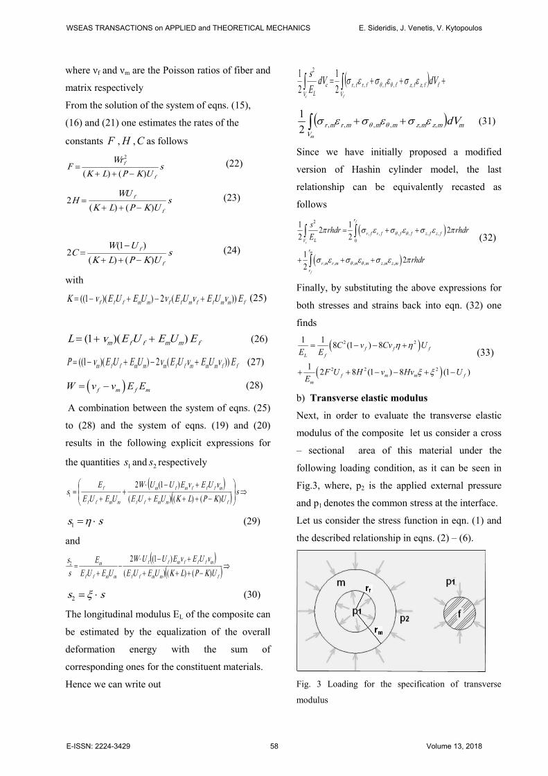
b) Transverse elastic modulus

Next, in order to evaluate the transverse elastic

modulus of the composite let us consider a cross

– sectional area of this material under the

following loading condition, as it can be seen in

Fig.3, where, p2 is the applied external pressure

and p1 denotes the common stress at the interface.

Let us consider the stress function in eqn. (1) and

the described relationship in eqns. (2) – (6).

Fig. 3 Loading for the specification of transverse

modulus

WSEAS TRANSACTIONS on APPLIED and THEORETICAL MECHANICS E. Sideridis, J. Venetis, V. Kytopoulos

E-ISSN: 2224-3429 58 Volume 13, 2018

The boundary conditions are formulated as

follows

fr r= : , , 1 12 2r f r mf

Fp H pr

σ σ= = − → + = − (34)

mr r= : , 2 222r m

m

Fp H p

rσ = − → + = − (35)

Hence the constants F and H are estimated as

( )( )2

2 12 2

f m

m f

p p r rF

r r−

=−

(36)

and

( )2 21 2

2 22 f m

m f

p r p rH

r r−

=−

(37)

Moreover, in the present analysis we have also

assumed that the axial strains are a priori

negligible, and therefore

( ), , , ,0z f z f f r f fv θε σ σ σ= → = + (38a)

( ), , , ,0z m z m m r m mv θε σ σ σ= → = + (38b)

Besides, from the stress – strain relationships we

have

( )2

, ,

2 1 2f ff r f

f

C v vEθε ε− −

= = (39a)

( ) ( )2, 2

1 1 2 1 2m m m mm

F v H v vE rθε

= − + + − − (39b)

( ) ( )2, 2

1 1 2 1 2r m m m mm

F v H v vE r

ε = + + − − (39c)

Concurrently, the following relationships hold

, ,r f fu r θε= , , ,r m mu r θε=

Also, at fr r= it implies that

, ,r f r mu u= (40)

Consequently, we infer

( ) ( ) ( )2 222 1 2 1 2 1 2f f m f m m mf

FC v v E E v H v vr

− − = − + + − −

(41)

Apparently, if one substitutes the rates of the

quantities F and 2H back into eqn. (41) a linear

algebraic expression between the magnitudes of

the pressures 1p and 2p arises.

Hence we can write out

1 2p pλ=

with

( ) 2

2(1 )(1 )

(1 ) (1 2 ) 1 (1 2 )(1 )m m f

m m f f f f f m

v v E

v v U E v U Eλ

ν

+ −=

+ − + + − − −(42)

The transverse elastic modulus is calculated from

the eq. (31), by setting on its left member instead

of the integral ∫cV

cdVEs

2

21

the terms in the

quantity ∫cV

cc

dVKp2

2

21

, where 2p is the initially

imposed pressure and cK denotes the bulk

modulus of the composite, which is evaluated by

means of the following expression

−

−=

L

LT

T

TTc

Ev

Ev

K2212

1

Since

( ) zL

LTyTTx

Tx E

vvE

σσσε

−−=

1

( ) zL

LTxTTy

Ty E

vvE

σσσε

−−=

1

( )1z z LT x y

L

vE

ε σ σ σ = − +

2x y pσ σ= = − and 0zε =

where TE denotes the transverse elastic modulus.

WSEAS TRANSACTIONS on APPLIED and THEORETICAL MECHANICS E. Sideridis, J. Venetis, V. Kytopoulos

E-ISSN: 2224-3429 59 Volume 13, 2018

and LTv , TTv are the longitudinal and

transverse Poisson ratio respectively

Thus, by substituting the resultant relationships

for the strains, the stresses and the unknown

constants together with the auxiliary term λ back

into eqn. (32) which is modified properly in order

to include at the left member the expression with

Kc and p2 one obtains the following explicit

expression for the transverse elastic modulus 2 2 2 2

2

2 2 2

2

(1 2 ) (1 2 )( 1)1

(1 ) (1 ) (1 )

(1 )(1 ) 2

(1 ) (1 ) (1 )

f f f m m f

T f T T m f TT

f m LT

m f T T L T T

U v v v v U

E E v E U v

U v v

E U v E v

λ λ

λ

− − − − −= + +

− − −

+ −+

− − −

(43a)

c) Longitudinal Poisson ratio

Next, the longitudinal Poisson ratio can be

evaluated by means of the following reasoning.

It is valid that

r mLT

z

d rvε

= −

where rd denotes the radial displacement in the

cylindrical area of the composite and zε is the

axial displacement.

Thus 2

2,

, 2

/ (1 ) 2 (1 )( ) /4

m m m m mr m r r mLT

z m m

F r v H v v su rv

s Hvε=

− + + − − = − =−

(43b)

A substitution of eqns. (22), (23), (30), back into

(43b), leads to the following closed – form

relationship

(43c)

d) Transverse Poisson ratio

Moreover, the transverse Poisson ratio of the

composite can be estimated by means of Halpin –

Tsai equation which is presented as follows:

f

fmTT U

Uvv

⋅−⋅⋅+

=1

11

11

ηηξ

(44)

where:

mf

mf

vv

νξν

η1

1 +−

=

and

...3,2,11 =ξ

e) Shear Modulus

On the other hand, to define shear modulus one

can take into account Halpin – Tsai formula i.e.

f

fmLT U

UGG

⋅−⋅⋅+

=2

22

11

ηηξ

(45)

where

mf

mf

GGGG

22 ξ

η+−

=

and 2ξ is a constant term which depends on the

fiber volume fraction and arises from the

following empirical relationship 10f2 U401ξ ⋅+=

Here mf GG , are the shear moduli of fiber and

matrix respectively.

Besides, Hashin and Rosen proposed the

following expression concerning the shear

modulus of a composite was proposed

])()[(])()[(

fmfmf

fmfmfmLT UGGGG

UGGGGGG

⋅−−+

⋅−++= (46)

In continuing, to introduce the discontinuity of

fibers we will use the model of equivalent fiber,

which is described as follows:

Let us suppose a composite material consisting of

unidirectional discontinuous fibers

WSEAS TRANSACTIONS on APPLIED and THEORETICAL MECHANICS E. Sideridis, J. Venetis, V. Kytopoulos

E-ISSN: 2224-3429 60 Volume 13, 2018

Fig. 4 Arrangement of the short fibers in the matrix

Next, let as focus on the cross – sectional area of a

representative volume element of this material.

Fig. 5 Cross – sectional area of an arbitrary short

fiber of the composite

We transform the above volume element in order

to create another volume element consisting of an

equivalent fiber

Fig. 6 Cross – sectional area of the equivalent fiber

Here, we should emphasize that the real system

consisting of short fibers and matrix is

characterized by the elastic

constants fE , mE , fU , mU whereas the equivalent

system consisting equivalent fiber and matrix, is

described by the constants meqfeqmfeq UUEE ,,, .

In this context, let as c alculate the fundamental

elastic properties of the composite.

Primarily, we have to estimate the filler content

which in the real system is given as

ll

dd

Ul

d

ld

U fff

ff

f ⋅=⇒⋅⋅

⋅⋅= 2

2

2

2

4

4

π

π (47)

and in the equivalent system

2

2

2

2

4

4dd

Ul

d

ld

U ffeq

f

f =⇒⋅⋅

⋅⋅=π

π (48)

Hence,

ff

feq UllU ⋅= (49)

To evaluate the elastic modulus of equivalent

fiber, one may adopt the Strength of Materials

approach according to which the system filler –

matrix is equivalent with a system of two ideal

springs connected in series. Evidently, this

implies that the exerted force is the same both for

matrix and filler, while their lengthening differs,

as it can be seen in Fig. 7

Fig. 7 S trength of materials approach for the

simulation of equivalent fiber

f mF F F= = and ( ) ( )f ml l l∆ = ∆ + ∆

Moreover the following relationships hold,

F σ= ⋅Α , f f fF σ= ⋅Α

m m mF σ= ⋅Α , feqEσ ε= ⋅

f f fEσ ε= ⋅ , m m mEσ ε= ⋅

( ) m mml lε∆ = ⋅

and therefore,

( ) f ffl lε∆ = ⋅

WSEAS TRANSACTIONS on APPLIED and THEORETICAL MECHANICS E. Sideridis, J. Venetis, V. Kytopoulos

E-ISSN: 2224-3429 61 Volume 13, 2018

f f m m f f m m f f m ml l l l l V l V V Vε ε ε ε ε ε ε ε ε⋅ = ⋅ + ⋅ ⇒ ⋅ = ⋅ ⋅ + ⋅ ⋅ ⇒ = ⋅ + ⋅ ⇒

f f m m

feq f m

l lE E l E l

σ σσ ⋅ ⋅= +

⋅ ⋅ (50)

Besides, referring to the equivalent fiber the

following equality holds

f mσ σ σ= =

Consequently we find

m ffeq

f mm f

E EE l lE E

l l

⋅=

⋅ + ⋅ (51)

To calculate Poisson ratio of the equivalent fiber

we may consider without violating the generality

of our presented mathematical formalism, that the

overall lengthening and the dilatation of this

hypothetical fiber are equal with the sum and the

average of the real fiber and matrix respectively.

The overall lengthening is

1 1f m

f f m m f m

l ll l ll l

ε ε ε ε ε ε⋅ = ⋅ + ⋅ ⇒ = ⋅ + ⋅ (52)

whereas the dilatation is given as

2f m

f f m m

l lv vl l

ε ε ε= − ⋅ ⋅ − ⋅ ⋅ (53)

Since 2

1feqv ε

ε= − we have

1

1

m f f mf

feq

m ff

lE El

vlE El

ν ν

⋅ + ⋅ ⋅ − =

+ ⋅ −

(54)

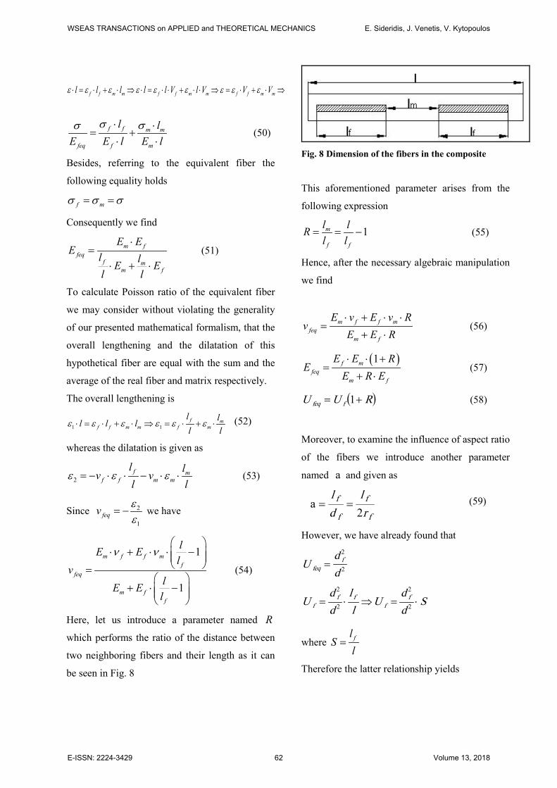
Here, let us introduce a parameter named R

which performs the ratio of the distance between

two neighboring fibers and their length as it can

be seen in Fig. 8

Fig. 8 Dimension of the fibers in the composite

This aforementioned parameter arises from the

following expression

1m

f f

l lRl l

= = − (55)

Hence, after the necessary algebraic manipulation

we find

m f f mfeq

m f

E v E v Rv

E E R⋅ + ⋅ ⋅

=+ ⋅

(56)

( )1f mfeq

m f

E E RE

E R E⋅ ⋅ +

=+ ⋅

(57)

( )RUU ffeq += 1 (58)

Moreover, to examine the influence of aspect ratio

of the fibers we introduce another parameter

named a and given as

f

f

f

f

rl

dl

2a == (59)

However, we have already found that

Sdd

Ull

dd

U

dd

U

ff

fff

ffeq

⋅=⇒⋅=

=

2

2

2

2

2

2

where flS

l=

Therefore the latter relationship yields

WSEAS TRANSACTIONS on APPLIED and THEORETICAL MECHANICS E. Sideridis, J. Venetis, V. Kytopoulos

E-ISSN: 2224-3429 62 Volume 13, 2018

⇒⋅⋅=⋅

⇒⋅=⋅⇒⋅=

Sdl

ll

U

Sdl

Udl

ld

U

ff

ff

f

f

ff

2

2

2

222

2

222

2

2

2

2

a

a

2322a

=⋅

dlSU f (60)

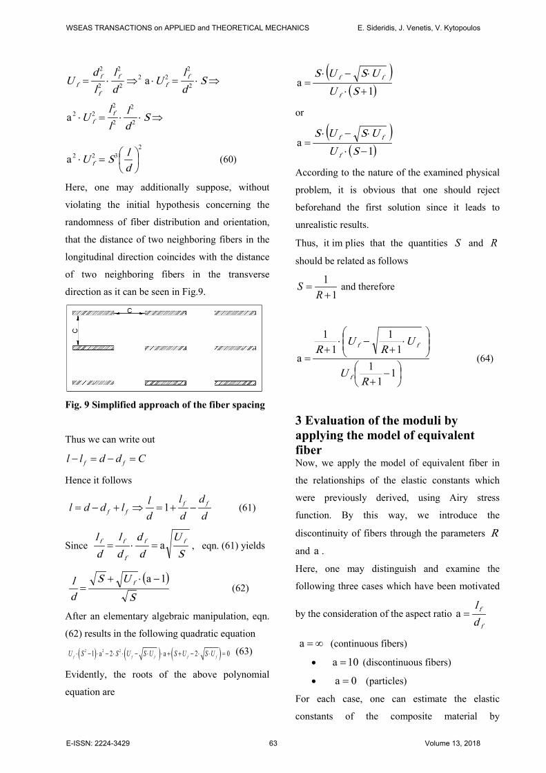
Here, one may additionally suppose, without

violating the initial hypothesis concerning the

randomness of fiber distribution and orientation,

that the distance of two neighboring fibers in the

longitudinal direction coincides with the distance

of two neighboring fibers in the transverse

direction as it can be seen in Fig.9.

Fig. 9 Simplified approach of the fiber spacing

Thus we can write out

f fl l d d C− = − =

Hence it follows

1 f ff f

l dll d d ld d d

= − + ⇒ = + − (61)

Since S

Udd

dl

dl ff

f

ff a=⋅= , eqn. (61) yields

( )

SUS

dl f 1a −⋅+= (62)

After an elementary algebraic manipulation, eqn.

(62) results in the following quadratic equation

( ) ( ) ( )2 2 21 a 2 a 2 0f f f f fU S S U S U S U S U⋅ − ⋅ − ⋅ ⋅ − ⋅ ⋅ + + − ⋅ ⋅ = (63)

Evidently, the roots of the above polynomial

equation are

( )( )1

a+⋅

⋅−⋅=

SUUSUS

f

ff

or

( )( )1

a−⋅

⋅−⋅=

SUUSUS

f

ff

According to the nature of the examined physical

problem, it is obvious that one should reject

beforehand the first solution since it leads to

unrealistic results.

Thus, it im plies that the quantities S and R

should be related as follows

11

SR

=+

and therefore

−

+

⋅

+−⋅

+=

11

11

11

1

a

RU

UR

UR

f

ff

(64)

3 Evaluation of the moduli by applying the model of equivalent fiber Now, we apply the model of equivalent fiber in

the relationships of the elastic constants which

were previously derived, using Airy stress

function. By this way, we introduce the

discontinuity of fibers through the parameters R

and a .

Here, one may distinguish and examine the

following three cases which have been motivated

by the consideration of the aspect ratio f

f

dl

=a

∞=a (continuous fibers)

• 10a = (discontinuous fibers)

• 0a = (particles)

For each case, one can estimate the elastic

constants of the composite material by

WSEAS TRANSACTIONS on APPLIED and THEORETICAL MECHANICS E. Sideridis, J. Venetis, V. Kytopoulos

E-ISSN: 2224-3429 63 Volume 13, 2018

substituting the quantities fE , fv , fU , fG , mU

which appear in eqns. (33), (43a), (43c) and (46)

back into eqns. (51), (54) (56), (57), (58) which

describe the simulation of equivalent fiber and

contain the terms f eqE , f eqv , feqU , f eqG , meqU .

Consequently, in regards to the longitudinal

elastic modulus one obtains

( )

( )

2 2

2 2 2

8 (1 ) 8

12 (1 ) 8 (1 ) 8 (1 )

1 1

eq eq eq eq

eq eq eq eq eq eq f

eq feq m m m feqm

Leq feq

C v C v U

F U v H v H v UE

E Eη η

ξ ξ

− − +

+ + + − − + −

= (65)

According to the same reasoning, the transverse

elastic modulus arises from the following

expression 2 2 2 2

2

2 2 2

2

(1 2 ) (1 2 )( 1)1(1 ) (1 ) (1 )

(1 )(1 ) 2(1 ) (1 ) (1 )

feq f feq eq m m eq feq

Teq feq Teq m feq Teq

feq m eq LTeq

m f Teq L Teq

U v v v v UE E v E U v

U v vE U v E v

λ λ

λ

− − − − −= +

− − −

+ −+ +

− − −

(66)

Moreover, the longitudinal Poisson ratio and the

shear modulus are respectively estimated as ( )

mmmfeqfeqfeqeqmfeqfeqfeqmfeqfeqeqfeqeqeqeqeqm

mmfeqfeqfeqmfeqfeqeqfeqeqeqeqeqmmmfeqfeqfeqeqLTeq KPLK

KPLKν)UEUE(U2W)νEUνE)U1((UW2)U)()((Eν)νEUνE)U1((UW2)U)()((E)UEUE(U2W

ν+++−−−++

+−−−++++=

(67)

and

[( ) ( ) ]

[( ) ( ) ]feq m feq m feq

LT eq mfeq m feq m feq

G G G G UG G

G G G G U

+ + − ⋅=

+ − − ⋅ (68)

4 Numerical Examples The numerical results of the above theoretical

expressions are presented in the following tables,

using the following fiber and matrix properties

fE = 72 G Pa, mE =3.5 GPa, mv =0.36, fG =30

Gpa, mG =1.3 Gpa

First case: ∞=⇒= a0R (continuous fibers).

65.0=fU

f eqE f eqv f eqG feqU meqU

7.2 1010 N / m2 0.2 3.1010 N / m2 0.65 0,35

Table 1 Elastic constants for ∞=⇒= a0R

fU LeqE (N

/m2) T eqE (N

/m2) LT eqG (

N/m2) LT eqv

0 3.5E+9 3.5E+9 1.287E+9 0.36

0.1 1.038E+10

5.541E+9

1.547E+9 0.341

0.2 1.725E+10

6.976E+9

1.865E+9 0.322

0.3 2.412E+10

8.493E+9

2.265E+9 0.304

0.4 3.097E+10

1.031E+10

2.779E+9 0.287

0.5 3.782E+10

1.262E+10

3.469E+9 0.271

0.6 4.467E+10

1.575E+10 4.44E+9 0.256

0.7 5.15E+10

2.026E+10 5.91E+9 0.241

0.8 5.834E+10

2.739E+10

8.395E+9 0.227

0.9 6.517E+10

4.043E+10

1.35E+10 0.213

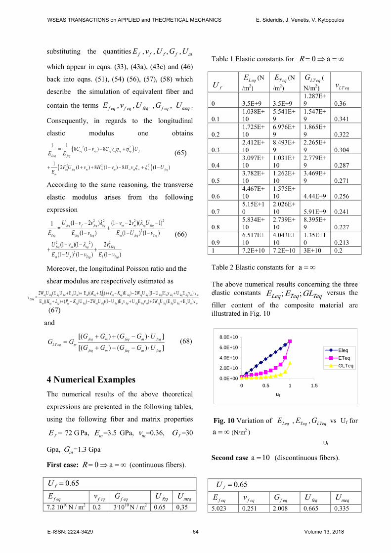
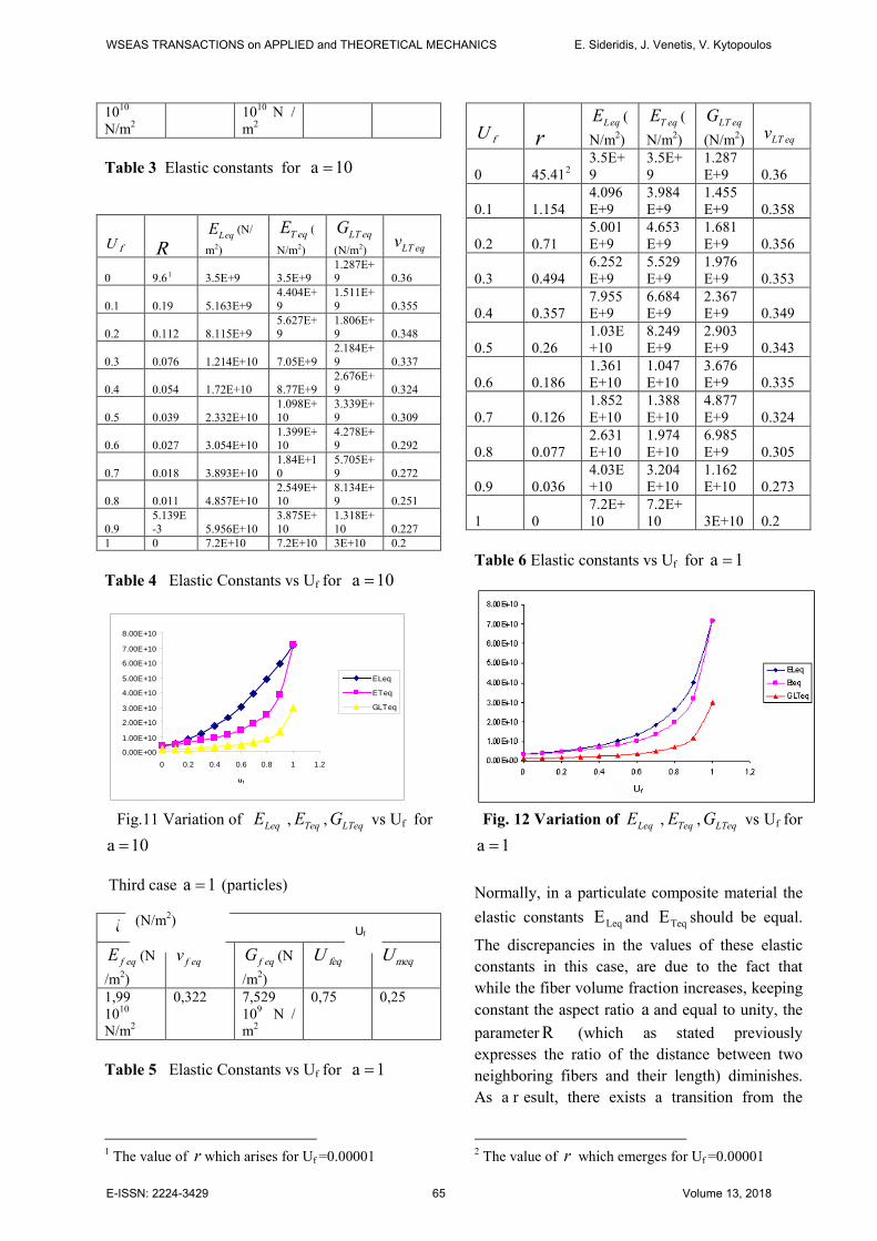
1 7.2E+10 7.2E+10 3E+10 0.2 Table 2 Elastic constants for ∞=a The above numerical results concerning the three elastic constants TeqTeqLeq GLEE ;; versus the

filler content of the composite material are illustrated in Fig. 10

0.0E+00

2.0E+10

4.0E+10

6.0E+10

8.0E+10

0 0.5 1 1.5

uf

EleqETeqGLTeq

Fig. 10 Variation of LeqE , TeqE , LTeqG vs Uf for

∞=a . Second case 10a = (discontinuous fibers).

65.0=fU

f eqE f eqv f eqG feqU meqU

5.023 0.251 2.008 0.665 0.335

Uf

(N/m2 )

WSEAS TRANSACTIONS on APPLIED and THEORETICAL MECHANICS E. Sideridis, J. Venetis, V. Kytopoulos

E-ISSN: 2224-3429 64 Volume 13, 2018

1010

N/m2 1010 N / m2

Table 3 Elastic constants for 10a =

fU R LeqE (N/

m2) T eqE (

N/m2) LT eqG

(N/m2) LT eqv

0 9.61 3.5E+9 3.5E+9 1.287E+9 0.36

0.1 0.19 5.163E+9 4.404E+9

1.511E+9 0.355

0.2 0.112 8.115E+9 5.627E+9

1.806E+9 0.348

0.3 0.076 1.214E+10 7.05E+9 2.184E+9 0.337

0.4 0.054 1.72E+10 8.77E+9 2.676E+9 0.324

0.5 0.039 2.332E+10 1.098E+10

3.339E+9 0.309

0.6 0.027 3.054E+10 1.399E+10

4.278E+9 0.292

0.7 0.018 3.893E+10 1.84E+10

5.705E+9 0.272

0.8 0.011 4.857E+10 2.549E+10

8.134E+9 0.251

0.9 5.139E-3 5.956E+10

3.875E+10

1.318E+10 0.227

1 0 7.2E+10 7.2E+10 3E+10 0.2 Table 4 Elastic Constants vs Uf for 10a =

0.00E+00

1.00E+10

2.00E+10

3.00E+10

4.00E+10

5.00E+10

6.00E+10

7.00E+10

8.00E+10

0 0.2 0.4 0.6 0.8 1 1.2

uf

ELeq

ETeq

GLTeq

Fig.11 Variation of LeqE , TeqE , LTeqG vs Uf for

10 a = Third case 1a = (particles)

65.0=fU

f eqE (N/m2)

f eqv f eqG (N/m2)

feqU meqU

1,99 1010

N/m2

0,322 7,529 109 N / m2

0,75 0,25

Table 5 Elastic Constants vs Uf for 1a =

1 The value of r which arises for Uf =0.00001

fU r LeqE (

N/m2) T eqE (

N/m2) LT eqG

(N/m2) LT eqv

0 45.412 3.5E+9

3.5E+9

1.287E+9 0.36

0.1 1.154 4.096E+9

3.984E+9

1.455E+9 0.358

0.2 0.71 5.001E+9

4.653E+9

1.681E+9 0.356

0.3 0.494 6.252E+9

5.529E+9

1.976E+9 0.353

0.4 0.357 7.955E+9

6.684E+9

2.367E+9 0.349

0.5 0.26 1.03E+10

8.249E+9

2.903E+9 0.343

0.6 0.186 1.361E+10

1.047E+10

3.676E+9 0.335

0.7 0.126 1.852E+10

1.388E+10

4.877E+9 0.324

0.8 0.077 2.631E+10

1.974E+10

6.985E+9 0.305

0.9 0.036 4.03E+10

3.204E+10

1.162E+10 0.273

1 0 7.2E+10

7.2E+10 3E+10 0.2

Table 6 Elastic constants vs Uf for 1a =

Fig. 12 Variation of LeqE , TeqE , LTeqG vs Uf for

1a =

Normally, in a particulate composite material the elastic constants LeqE and TeqE should be equal.

The discrepancies in the values of these elastic constants in this case, are due to the fact that while the fiber volume fraction increases, keeping constant the aspect ratio a and equal to unity, the parameter R (which as stated previously expresses the ratio of the distance between two neighboring fibers and their length) diminishes. As a r esult, there exists a transition from the

2 The value of r which emerges for Uf =0.00001

Uf

(N/m2)

WSEAS TRANSACTIONS on APPLIED and THEORETICAL MECHANICS E. Sideridis, J. Venetis, V. Kytopoulos

E-ISSN: 2224-3429 65 Volume 13, 2018

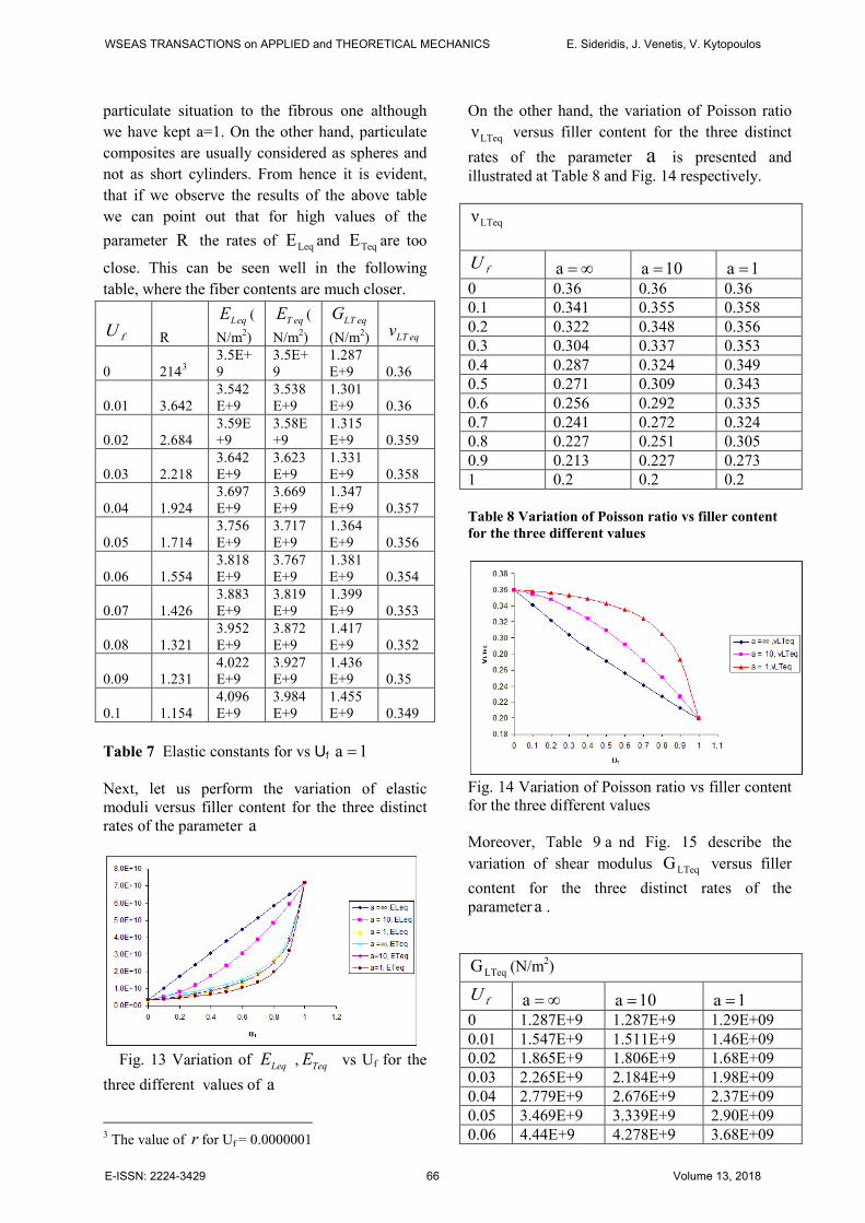
particulate situation to the fibrous one although we have kept a=1. On the other hand, particulate composites are usually considered as spheres and not as short cylinders. From hence it is evident, that if we observe the results of the above table we can point out that for high values of the parameter R the rates of LeqE and TeqE are too

close. This can be seen well in the following table, where the fiber contents are much closer.

fU R LeqE (

N/m2) T eqE (

N/m2) LT eqG

(N/m2) LT eqv

0 2143 3.5E+9

3.5E+9

1.287E+9 0.36

0.01 3.642 3.542E+9

3.538E+9

1.301E+9 0.36

0.02 2.684 3.59E+9

3.58E+9

1.315E+9 0.359

0.03 2.218 3.642E+9

3.623E+9

1.331E+9 0.358

0.04 1.924 3.697E+9

3.669E+9

1.347E+9 0.357

0.05 1.714 3.756E+9

3.717E+9

1.364E+9 0.356

0.06 1.554 3.818E+9

3.767E+9

1.381E+9 0.354

0.07 1.426 3.883E+9

3.819E+9

1.399E+9 0.353

0.08 1.321 3.952E+9

3.872E+9

1.417E+9 0.352

0.09 1.231 4.022E+9

3.927E+9

1.436E+9 0.35

0.1 1.154 4.096E+9

3.984E+9

1.455E+9 0.349

Table 7 Elastic constants for vs Uf 1a = Next, let us perform the variation of elastic moduli versus filler content for the three distinct rates of the parameter a

Fig. 13 Variation of LeqE , TeqE vs Uf for the three different values of a

3 The value of r for Uf = 0.0000001

On the other hand, the variation of Poisson ratio LTeqν versus filler content for the three distinct

rates of the parameter a is presented and illustrated at Table 8 and Fig. 14 respectively.

LTeqν

fU ∞=a 10a = 1a = 0 0.36 0.36 0.36 0.1 0.341 0.355 0.358 0.2 0.322 0.348 0.356 0.3 0.304 0.337 0.353 0.4 0.287 0.324 0.349 0.5 0.271 0.309 0.343 0.6 0.256 0.292 0.335 0.7 0.241 0.272 0.324 0.8 0.227 0.251 0.305 0.9 0.213 0.227 0.273 1 0.2 0.2 0.2 Table 8 Variation of Poisson ratio vs filler content for the three different values

Fig. 14 Variation of Poisson ratio vs filler content for the three different values Moreover, Table 9 a nd Fig. 15 describe the variation of shear modulus LTeqG versus filler content for the three distinct rates of the parameter a .

LTeqG (N/m2)

fU ∞=a 10a = 1a = 0 1.287E+9 1.287E+9 1.29E+09 0.01 1.547E+9 1.511E+9 1.46E+09 0.02 1.865E+9 1.806E+9 1.68E+09 0.03 2.265E+9 2.184E+9 1.98E+09 0.04 2.779E+9 2.676E+9 2.37E+09 0.05 3.469E+9 3.339E+9 2.90E+09 0.06 4.44E+9 4.278E+9 3.68E+09

WSEAS TRANSACTIONS on APPLIED and THEORETICAL MECHANICS E. Sideridis, J. Venetis, V. Kytopoulos

E-ISSN: 2224-3429 66 Volume 13, 2018

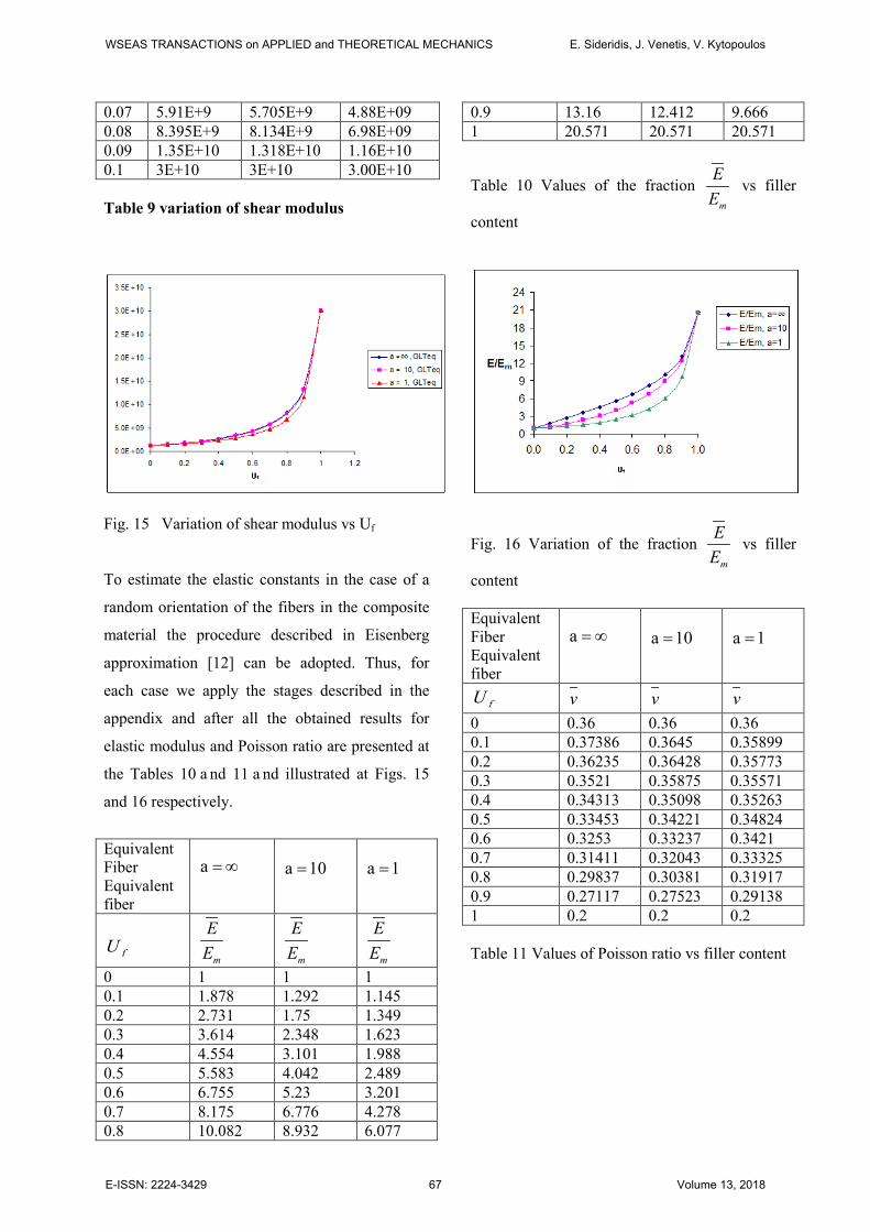
0.07 5.91E+9 5.705E+9 4.88E+09 0.08 8.395E+9 8.134E+9 6.98E+09 0.09 1.35E+10 1.318E+10 1.16E+10 0.1 3E+10 3E+10 3.00E+10 Table 9 variation of shear modulus

Fig. 15 Variation of shear modulus vs Uf To estimate the elastic constants in the case of a

random orientation of the fibers in the composite

material the procedure described in Eisenberg

approximation [12] can be adopted. Thus, for

each case we apply the stages described in the

appendix and after all the obtained results for

elastic modulus and Poisson ratio are presented at

the Tables 10 a nd 11 a nd illustrated at Figs. 15

and 16 respectively.

Equivalent Fiber Equivalent fiber

∞=a

10a =

1a =

fU m

EE

m

EE

m

EE

0 1 1 1 0.1 1.878 1.292 1.145 0.2 2.731 1.75 1.349 0.3 3.614 2.348 1.623 0.4 4.554 3.101 1.988 0.5 5.583 4.042 2.489 0.6 6.755 5.23 3.201 0.7 8.175 6.776 4.278 0.8 10.082 8.932 6.077

0.9 13.16 12.412 9.666 1 20.571 20.571 20.571

Table 10 Values of the fraction m

EE

vs filler

content

Fig. 16 Variation of the fraction m

EE

vs filler

content Equivalent Fiber Equivalent fiber

∞=a

10a =

1a =

fU v v v 0 0.36 0.36 0.36 0.1 0.37386 0.3645 0.35899 0.2 0.36235 0.36428 0.35773 0.3 0.3521 0.35875 0.35571 0.4 0.34313 0.35098 0.35263 0.5 0.33453 0.34221 0.34824 0.6 0.3253 0.33237 0.3421 0.7 0.31411 0.32043 0.33325 0.8 0.29837 0.30381 0.31917 0.9 0.27117 0.27523 0.29138 1 0.2 0.2 0.2 Table 11 Values of Poisson ratio vs filler content

WSEAS TRANSACTIONS on APPLIED and THEORETICAL MECHANICS E. Sideridis, J. Venetis, V. Kytopoulos

E-ISSN: 2224-3429 67 Volume 13, 2018

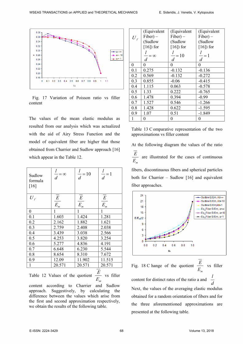
Fig. 17 Variation of Poisson ratio vs filler content The values of the mean elastic modulus as

resulted from our analysis which was actualized

with the aid of Airy Stress Function and the

model of equivalent fiber are higher that those

obtained from Charrier and Sudlow approach [16]

which appear in the Table 12.

Sudlow formula [16]

ld= ∞ 10l

d= 1l

d=

fU

m

EE

m

EE

m

EE

0 1 1 1 0.1 1.603 1.424 1.281 0.2 2.162 1.882 1.621 0.3 2.759 2.408 2.038 0.4 3.439 3.038 2.566 0.5 4.253 3.820 3.254 0.6 5.277 4.836 4.191 0.7 6.648 6.230 5.544 0.8 8.654 8.310 7.672 0.9 12.09 11.902 11.515 1 20.571 20.571 20.571

Table 12 Values of the quotient mE

E vs filler

content according to Charrier and Sudlow approach. Suggestively, by calculating the difference between the values which arise from the first and second approximation respectively, we obtain the results of the following table.

fU (Equivalent Fiber) – (Sudlow [16]) for ld= ∞

(Equivalent Fiber) – (Sudlow [16]) for

10ld=

(Equivalent Fiber) –(Sudlow [16]) for

1ld=

0 0 0 0 0.1 0.275 -0.132 -0.136 0.2 0.569 -0.132 -0.272 0.3 0.855 -0.06 -0.415 0.4 1.115 0.063 -0.578 0.5 1.33 0.222 -0.765 0.6 1.478 0.394 -0.99 0.7 1.527 0.546 -1.266 0.8 1.428 0.622 -1.595 0.9 1.07 0.51 -1.849 1 0 0 0 Table 13 C omparative representation of the two approximations vs filler content At the following diagram the values of the ratio

m

EE

are illustrated for the cases of continuous

fibers, discontinuous fibers and spherical particles

both for Charrier – Sudlow [16] and equivalent

fiber approaches.

Fig. 18 C hange of the quotient m

EE

vs filler

content for distinct rates of the ratio a and ld

Next, the values of the averaging elastic modulus

obtained for a random orientation of fibers and for

the three aforementioned approximations are

presented at the following table.

WSEAS TRANSACTIONS on APPLIED and THEORETICAL MECHANICS E. Sideridis, J. Venetis, V. Kytopoulos

E-ISSN: 2224-3429 68 Volume 13, 2018

Sudlow approach [16]

Eisenberg approach [12]

Equivalent fiber approach

ld= ∞ ,

1lC =

∞=a

fU m

EE

m

EE

m

EE

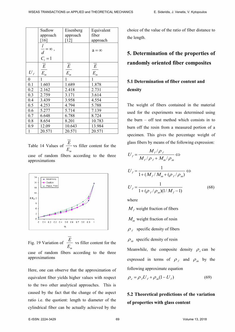
0 1 1 1 0.1 1.603 1.689 1.878 0.2 2.162 2.418 2.731 0.3 2.759 3.171 3.614 0.4 3.439 3.958 4.554 0.5 4.253 4.794 5.788 0.6 5.277 5.714 7.139 0.7 6.648 6.788 8.724 0.8 8.654 8.201 10.783 0.9 12.09 10.643 13.984 1 20.571 20.571 20.571

Table 14 Values of m

EE

vs filler content for the

case of random fibers according to the three approximations

Fig. 19 Variation of m

EE

vs filler content for the

case of random fibers according to the three approximations

Here, one can observe that the approximation of

equivalent fiber yields higher values with respect

to the two other analytical approaches. This is

caused by the fact that the change of the aspect

ratio i.e. the quotient: length to diameter of the

cylindrical fiber can be actually achieved by the

choice of the value of the ratio of fiber distance to

the length.

5. Determination of the properties of

randomly oriented fiber composites

5.1 Determination of fiber content and

density

The weight of fibers contained in the material

used for the experiments was determined using

the burn – off test method which consists in to

burn off the resin from a measured portion of a

specimen. This gives the percentage weight of

glass fibers by means of the following expression:

⇔+

=mmff

fff MM

MU

ρρρ

///

⇔++

=)/(/(1

1

mfmff MM

Uρρ

)1/1)(/(11

−+=

fmff M

Uρρ

(68)

where

fM weight fraction of fibers

mM weight fraction of resin

fρ specific density of fibers

mρ specific density of resin

Meanwhile, the composite density cρ can be

expressed in terms of fρ and mρ by the

following approximate equation

)1( fmffc UU −+= ρρρ (69)

5.2 Theoretical predictions of the variation

of properties with glass content

WSEAS TRANSACTIONS on APPLIED and THEORETICAL MECHANICS E. Sideridis, J. Venetis, V. Kytopoulos

E-ISSN: 2224-3429 69 Volume 13, 2018

To estimate the overall elastic modulus cE of a

glass fiber resin, the simple rule of mixtures can

be taken into consideration, which is usually

stated in the following form:

mmffec UEUEE +=η (70)

where eη is an efficiency factor depending on the

type and the fabrication of the reinforcement. This

simplified equation ignores the presence of voids

and of low modulus mat binding material but

usually is of adequate accuracy at this instance.

This equation, although by its nature only

approximate gives a feel of the qualitative effect

of the various parameters. Since, usually

mf EE >> , it is evident that the modulus of the

composite from the simple rule of mixtures will

increase with increasing filler content. Therefore,

with eq. (70) in hand and taking into account that

1=+ mf UU we obtain the following equation

fm

f

m

f

fmfemc

M

MEEEE

−+

−+=

ρρ

ρρη

1

)( (71)

On the other hand, Christensen equation [7] which has already been referred in the Introduction Unit has been derived from a more rigorous analysis of the micromechanics involved than the simple rule of mixtures.

2

13 3

(1 ) (1 )1927 (1 ) (1 )

f fD f m

f f m fm

f f m f

E UE U E

E U E UE

E U E U

−= +

+ + −+ − + +

(72)

The theory employs a quasi – isotropic model together with a geometric averaging technique to predict an asymptotic value for the elastic modulus of randomly reinforced short fiber composites, for the two – dimensional case, (i.e. when the fibers are aligned only in the plane of the laminate).

6. Experimental Work 6.1 Material and Method of Construction The material was manufactured by a commercial fabricator. The resin was a pre – accelerated isophthalic polyester used with a peroxide catalyst. The reinforcement was powder bound, E glass fiber, chopped strand mat (CSM) of various weights per layer with glass tissue. The panels were laid up on the plate so that the lower surface of the panel was always flat and relatively smooth. A gel coat consisting of resin with two layers of surface tissue was first applied to the glass, which had previously been coated with release agent. The layers of CSM were then added ensuring that each layer was well wetted – out with resin. Finally, a second resin – rich layer (RRL) with a s ingle piece of surface tissue was applied, mainly to improve the external appearance of the laminate. Most of the panels were post – cured for 48 hours at 50 0C. To evaluate the volume fraction of fibers, the burn – off test method was performed. 6.2 Testing of Materials At first, tests were carried out to determine the fiber content and the density of the composite materials used. A prismatic sample was cut from each unbroken specimen or from each broken tension specimen as close as possible to the site of fracture. The samples were measured and weighed before being placed in a furnace for several hours at 620 0C + 200C to “burn off” the resin. From the weigh of the residues assumed to be all glass, the fiber content by weight Mf and the volume fraction can be calculated for each specimen. The obtained value is the average of the three measurements. Similarly, prismatic samples of given dimensions and volume were cut from specimens and were weighed in order to determine the density of the materials tested. Tension tests were carried out on an Instron universal testing machine using Istron measuring and recording equipments. Load was measured by a strain gauge extensometer of 25 mm gauge length. The extensometer was attached to one surface of the specimen which was loaded to approximately 0.3% strain and unloaded. Then, without removing the extensometer, the specimen the specimen was loaded to failure at a rate of 0.2 cm/min. Thus the main information sought, the initial stress data and the ultimate strength data, was obtained. In each case, the properties were

WSEAS TRANSACTIONS on APPLIED and THEORETICAL MECHANICS E. Sideridis, J. Venetis, V. Kytopoulos

E-ISSN: 2224-3429 70 Volume 13, 2018

expressed in terms of the elastic modulus and ultimate tensile stress. Values of ultimate strain were also measured. Again, the obtained values are the average of the three measurements. Specimens were cut from material panels with nine layers of CSM having a nominal thickness of 1 cm and they were taken from each of the two perpendicular directions using a band – saw. The edges of the specimens were machined in a milling machine to the shape of a dog bone specimen having total length 150 mm and width 25.4 mm whereas at the narrow measuring area gauge length 60 mm and width 12.4 mm respectively according to BS 2782. Before testing, the width and thickness of each specimen were measured with a micrometer at three points inside the gouge length. F rom these measurements mean values of thickness and width were estimated of each specimen. 7. Results and Discussion The procedure of the burn – off test yielded the value of the mean weight fraction of the fiber as 0.31. In continuing, by the aid of eq. (68) and using the values 3/2560 mKgf =ρ and

3/1100 mKgm =ρ the mean fiber volume fraction was evaluated as 172.0 . As to the density of the composite, it has been estimated experimentally by weighting pieces of given dimensions and dividing the weight by the volume. The mean value was 3/1419 mKgc =ρ . Besides, the theoretical value of the composite density calculated from eq. (69) using the above mentioned numerical values, can be found as 3/1426 mKgc =ρ . Here, one can pinpoint that there exists a s light discrepancy between these two values which partly can be attributed to the difficulty of determining the mean thickness of the sample pieces since, as mentioned previously, they varied significantly. The main properties of the CSM composite are presented in the Table 15.

Material

t(cm) Mf Uf

σu (MN/m) εu

Eexp(GN/m2)

Rule of mixture

s E(GN/

m2)

Christensen

formula E(GN/

m2)

1 0.87

0.32

0.181 105

0.015 9.31 7.75 8.66

2 0.96

0.29

0.161 110

0.018 8.19 7.46 8.30

3 0.94

0.30

0.167 114

0.018 8.51 7.62 8.50

4 0.90

0.31

0.174 104

0.015 8.77 7.75 8.66

Mean Value

0.92

0.31

0.171 108

0.017 8.70 8.70 8.70

Table 15 Main properties of the CSM composite

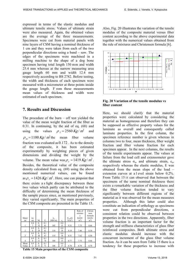
Also, Fig. 20 illustrates the variation of the tensile modulus of the composite material versus fiber content according to the above experimental data together with the numerical values obtained from the rule of mixtures and Christensen formula [6].

Fig. 20 Variation of the tensile modulus vs fiber content Here, we should clarify that the material properties were calculated by considering the material as homogeneous and therefore they can be supposed as effective property values for the laminate as overall and consequently called laminate properties. In the first column, the specimen reference number is given whereas in columns two to four, mean thickness, fiber weight fraction and fiber volume fraction for each specimen appear. In the next columns, the results of the tensile experiments appear. The values at failure from the load cell and extensometer gave the ultimate stress σu, and ultimate strain, εu, respectively whereas the elastic modulus, E was obtained from the mean slope of the load – extension curves at a l evel strain below 0.2%. From Table 15 i t can observed that between the specimens of the same nominal thickness there exists a remarkable variation of the thickness and the fiber volume fraction tended to vary significantly between different regions of the material as it was observed for the mean measures properties. Although this latter could also constitute an indication of orthology as specimens were cut from perpendicular directions, a consistent relation could be observed between properties in the two directions. Apparently, fiber volume fraction is an important factor for the strength and stiffness characteristics of glass fiber reinforced composites. Both ultimate stress and elastic modulus should increase with the concurrent increment of the glass fiber volume fraction. As it can be seen from Table 15 there is a tendency for these properties to increase with

WSEAS TRANSACTIONS on APPLIED and THEORETICAL MECHANICS E. Sideridis, J. Venetis, V. Kytopoulos

E-ISSN: 2224-3429 71 Volume 13, 2018

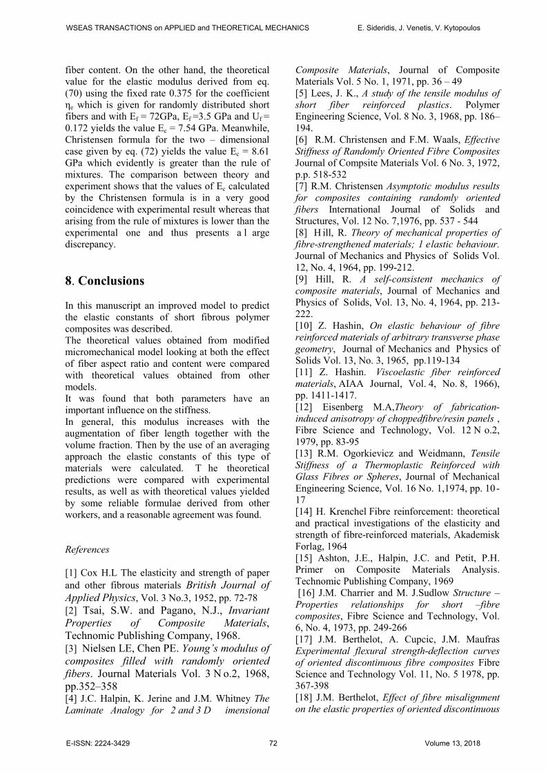
fiber content. On the other hand, the theoretical value for the elastic modulus derived from eq. (70) using the fixed rate 0.375 for the coefficient ηe which is given for randomly distributed short fibers and with Ef = 72GPa, Ef =3.5 GPa and Uf = 0.172 yields the value Ec = 7.54 GPa. Meanwhile, Christensen formula for the two – dimensional case given by eq. (72) yields the value Ec = 8.61 GPa which evidently is greater than the rule of mixtures. The comparison between theory and experiment shows that the values of Ec calculated by the Christensen formula is in a very good coincidence with experimental result whereas that arising from the rule of mixtures is lower than the experimental one and thus presents a l arge discrepancy. 8. Conclusions In this manuscript an improved model to predict the elastic constants of short fibrous polymer composites was described. The theoretical values obtained from modified micromechanical model looking at both the effect of fiber aspect ratio and content were compared with theoretical values obtained from other models. It was found that both parameters have an important influence on the stiffness. In general, this modulus increases with the augmentation of fiber length together with the volume fraction. Then by the use of an averaging approach the elastic constants of this type of materials were calculated. T he theoretical predictions were compared with experimental results, as well as with theoretical values yielded by some reliable formulae derived from other workers, and a reasonable agreement was found. References [1] Cox H.L The elasticity and strength of paper and other fibrous materials British Journal of Applied Physics, Vol. 3 No.3, 1952, pp. 72-78 [2] Tsai, S.W. and Pagano, N.J., Invariant Properties of Composite Materials, Technomic Publishing Company, 1968. [3] Nielsen LE, Chen PE. Young’s modulus of composites filled with randomly oriented fibers. Journal Materials Vol. 3 N o.2, 1968, pp.352–358 [4] J.C. Halpin, K. Jerine and J.M. Whitney The Laminate Analogy for 2 and 3 D imensional

Composite Materials, Journal of Composite Materials Vol. 5 No. 1, 1971, pp. 36 – 49 [5] Lees, J. K., A study of the tensile modulus of short fiber reinforced plastics. Polymer Engineering Science, Vol. 8 No. 3, 1968, pp. 186–194. [6] R.M. Christensen and F.M. Waals, Effective Stiffness of Randomly Oriented Fibre Composites Journal of Compsite Materials Vol. 6 No. 3, 1972, p.p. 518-532 [7] R.M. Christensen Asymptotic modulus results for composites containing randomly oriented fibers International Journal of Solids and Structures, Vol. 12 No. 7,1976, pp. 537 - 544 [8] H ill, R. Theory of mechanical properties of fibre-strengthened materials; 1 elastic behaviour. Journal of Mechanics and Physics of Solids Vol. 12, No. 4, 1964, pp. 199-212. [9] Hill, R. A self-consistent mechanics of composite materials, Journal of Mechanics and Physics of Solids, Vol. 13, No. 4, 1964, pp. 213-222. [10] Z. Hashin, On elastic behaviour of fibre reinforced materials of arbitrary transverse phase geometry, Journal of Mechanics and Physics of Solids Vol. 13, No. 3, 1965, pp.119-134 [11] Z. Hashin. Viscoelastic fiber reinforced materials, AIAA Journal, Vol. 4, No. 8, 1966), pp. 1411-1417. [12] Eisenberg M.A,Theory of fabrication-induced anisotropy of choppedfibre/resin panels , Fibre Science and Technology, Vol. 12 N o.2, 1979, pp. 83-95 [13] R.M. Ogorkievicz and Weidmann, Tensile Stiffness of a Thermoplastic Reinforced with Glass Fibres or Spheres, Journal of Mechanical Engineering Science, Vol. 16 No. 1,1974, pp. 10-17 [14] H. Krenchel Fibre reinforcement: theoretical and practical investigations of the elasticity and strength of fibre-reinforced materials, Akademisk Forlag, 1964 [15] Ashton, J.E., Halpin, J.C. and Petit, P.H. Primer on Composite Materials Analysis. Technomic Publishing Company, 1969 [16] J.M. Charrier and M. J.Sudlow Structure –Properties relationships for short –fibre composites, Fibre Science and Technology, Vol. 6, No. 4, 1973, pp. 249-266 [17] J.M. Berthelot, A. Cupcic, J.M. Maufras Experimental flexural strength-deflection curves of oriented discontinuous fibre composites Fibre Science and Technology Vol. 11, No. 5 1978, pp. 367-398 [18] J.M. Berthelot, Effect of fibre misalignment on the elastic properties of oriented discontinuous

WSEAS TRANSACTIONS on APPLIED and THEORETICAL MECHANICS E. Sideridis, J. Venetis, V. Kytopoulos

E-ISSN: 2224-3429 72 Volume 13, 2018

fibre composites, Fibre Science and Technology Vol. 17, No. 1, 1982, pp. 25 – 39 [19] Halpin, JC, and Tsai, SW. Environmental factors in composite materials. Technical Report AFML-TR. United State Air Force Materials Laboratory, 1969, 67-423. [20] Weng, G. J. and Sun, C. T., Effects of Fiber Length on E lastic Moduli of Randomly-Oriented Chopped-Fiber Composites, Composite Materials: Testing and Design (Fifth Conference), ASTM STP 674, S. W. Tsai, Ed., American Society for Testing and Materials, 1979, pp. 149-162. [21] A. G. Facca, M. T. Kortschot, and N. Yan, Predicting the elastic modulus of natural fibre reinforced thermoplastics,Composites Part A: Applied Science and Manufacturing, Vol. 37, No. 10, 2006, pp. 1660-1671 [22] G. Kalaprasad, K. Joseph, and S. Thomas, Theoretical modelling of tensile properties of short sisal fibre-reinforced low-density polyethylene composites, Journal of Materials Science, Vol.32, No. 16, 1997, pp 4261–4267 [23] J. C. Halpin and J. I. Kardos, The Halpin-Tsai equations: A review, Polymer Engineering and Science Vol. 16, No. 5, 1976 , pp. 344–352 [24] W.H. Bowyer, MG. Bader, On the reinforcement of thermoplastics by imperfectly aligned discontinuous fibres, Journal of Materials Science, Vol. 7, No. 11, 1972, pp 1315–1321 [25] L. Peponi, J. B iagiotti, M. Kenny, and I. Mondragon, Statistical analysis of the mechanical properties of natural fibers and their composite materials. II. Composite materials, Polymer Composites Vol. 29 No. 3, 2008, pp. 321–325. [26] J. Mirbagheri, M. Tajvidi, I. Ghasemi, and J. C. Hermanson, Prediction of the Elastic Modulus of Wood Flour/Kenaf Fibre/Polypropylene Hybrid Composites, Iranian Polymer Journal Vol. 16 No. 4, 2007, pp. 271-278 [27] S. Y. Fu, G. Xu, and Y.W. Mai, On the elastic modulus of hybrid particle/short-fiber/polymer composites, Composites Part B: Engineering Vol. 33, No. 4, 2002, pp. 291-299 [28] M. A. Islam and K. Begum, Prediction Models for the Elastic Modulus of Fiber-reinforced Polymer Composites: An Analysis, Journal of Scientific Research, Vol. 3, 2011, N o. 2, pp. 225-238 [29] J. Venetis and E. Sideridis Elastic constants of fibrous polymer composite materials reinforced with transversely isotropic fibers, AIP Advances Vol. 5, No. 3, 2015, Article ID 037118

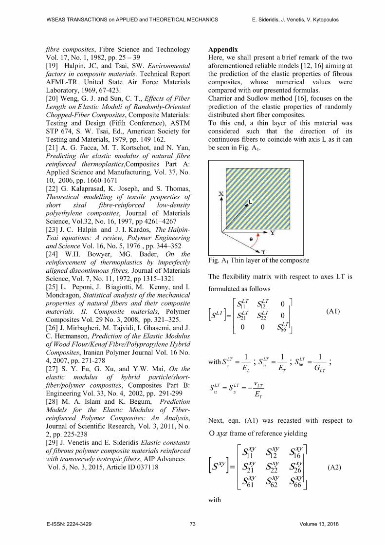
Appendix Here, we shall present a brief remark of the two aforementioned reliable models [12, 16] aiming at the prediction of the elastic properties of fibrous composites, whose numerical values were compared with our presented formulas. Charrier and Sudlow method [16], focuses on the prediction of the elastic properties of randomly distributed short fiber composites. To this end, a thin layer of this material was considered such that the direction of its continuous fibers to coincide with axis L as it can be seen in Fig. A1.

Fig. A1 Thin layer of the composite The flexibility matrix with respect to axes LT is

formulated as follows

[ ]

=LT

LTLT

LTLT

LT

SSSSS

S

66

2221

1211

0000

(A1)

with11

1LT

L

SE

= ;22

1LT

T

SE

= ; 661LT

LT

SG

= ;

12 21

LT LT LT

T

vS SE

= = −

Next, eqn. (A1) was recasted with respect to

xyzΟ frame of reference yielding

[ ]

=xyxyxy

xyxyxy

xyxyxy

xy

SSSSSSSSS

S

666261

262221

161211 (A2)

with

WSEAS TRANSACTIONS on APPLIED and THEORETICAL MECHANICS E. Sideridis, J. Venetis, V. Kytopoulos

E-ISSN: 2224-3429 73 Volume 13, 2018

11

4 4 2 2cos ( ) sin ( ) sin (2 ) 14

xy LT

L T LT L

vSE E G Eθ θ θ

= + + −

(A3) 4 4 2

222sin ( ) cos ( ) sin (2 ) 1

4xy LT

L T LT L

vSE E G Eθ θ θ

= + + −

(A4)

266

2 21 1 1 1 1cos (2 )xy LT LT

L L T L L T LT

v vS

E E E E E E Gθ= + + − + + −

(A5)

2

16

sin(2 )1 sin ( ) 1 2

2xy L L L

LT LT

L LT T LT

E E ES v v

E G E G

θθ= + − − + + −

(A6)

2

26

sin(2 )1 cos ( ) 1 2

2xy L L L

LT LT

L LT T LT

E E ES v v

E G E G

θθ= + − − + + −

(A7)

Here, to introduce the parameter of fiber

discontinuity it has been considered that the

fundamental elastic constants of the composite are

given by the following explicit representations

( )( )2( / ) 1 ( / ) 11

( / ) 2( / ) (( / ) 1)f m f

L mf m f m f

l d E E UE E

E E l d E E U

+ −= +

+ − −

(A8)

( )( )( / ) 2 ( / ) 11

(( / ) 1 ( / ) (( / ) 1))f m f

T m

f m f m f

d l E E UE E

E E d l E E U

+ −= +

+ + − −

(A9)

( )( )( / ) 2 ( / ) 11

(( / ) 1 ( / ) (( / ) 1))f m f

LT m

f m f m f

d l E E UG G

G G d l G G U

+ −= +

+ + − −

(A10)

ffmfLT vUvUv +−= )1( (A11)

where l ad= is the ratio between length and

diameter of a fiber, whereas the other quantities

have been already defined.

On the other hand, Eisenberg method [12] which also focuses on the prediction of the elastic properties of randomly distributed short fiber composites can be synopsized as follows. The stiffness matrix Q for an orthotropic layer of a

composite with respect to the principal material axes is defined as

[ ]

=

66

2221

1211

0000

QQQQQ

Q (A12)

Then a transformation of the matrix consisting of the coefficients ijQ to 'ijQ which corresponds to a turn of the rectangular Cartesian coordinate system at angle θ around zΟ axis.

[ ]

='66

'62

'61

'26

'22

'21

'16

'12

'11

QQQQQQQQQ

Q (A13)

with ' 4 4 2 211 11 22 12 66cos sin (2 4 )sin cosQ Q Q Q Qθ θ θ θ= + + +

' 4 4 2 222 11 22 12 66sin cos (2 4 )sin cosQ Q Q Q Qθ θ θ θ= + + +

' 2 2 2 2 266 11 22 12 66( 2 )sin cos (cos sin )Q Q Q Q Qθ θ θ θ= + − + −

' 2 2 4 412 11 22 66 12( 4 )sin cos (cos sin )Q Q Q Q Qθ θ θ θ= + − + +

' 2 2 2 216 11 22 12 66sin cos cos sin ( 2 )(sin cos )Q Q Q Q Qθ θ θ θ θ θ = − + + −

' 2 2 2 226 11 22 12 66sin cos sin cos ( 2 )(cos sin )Q Q Q Q Qθ θ θ θ θ θ = − + + −

Next, to evaluate the elastic constants of a composite layer with a random distribution of the short fibers, an averaging term of any of the above entries of the matrix 'Q is considered and therefore

'

0

1ij ijQ Q d

π

θπ

= ∫ (A14)

From hence it is evident that,

11 22 12 6611 221 (3 3 2 4 )8

Q Q Q Q Q Q= = + + + (A15)

11 22 12 66121 ( 6 4 )8

Q Q Q Q Q= + + − (A16)

11 22 12 66661 ( 2 4 )8

Q Q Q Q Q= + − + (A17)

16 26 0Q Q= = (A18) Referring to an isotropic material in a state of plane stress, the matrix Q is simplified as follows

WSEAS TRANSACTIONS on APPLIED and THEORETICAL MECHANICS E. Sideridis, J. Venetis, V. Kytopoulos

E-ISSN: 2224-3429 74 Volume 13, 2018

2 2

2 2

01 1

01 1

0 02(1 )

E vEv v

vE EQv v

Ev

− − = − − +

(A19)

After all, by equalizing the individual items of the above matrix with the quantities obtained from eqs. (A15) to (A18) one obtains

2 2

11 22 12 11 22 12 6611 12

11 22 12 6611

( 2 )( 2 4 )3 3 2 4

Q Q Q Q Q Q QQ QEQ Q Q QQ

+ + + − +−= =

+ + +(A20)

11 22 12 6612

11 22 12 6611

6 43 3 2 4Q Q Q QQvQ Q Q QQ

+ + −= =

+ + + (A21)

1 f f m mE E U E U= + (A22)

2f m

f f m m

E UE

E U E U=

+ (A23)

12 f f m mv v U v U= + (A24)

2(1 )f

ff

EG

v=

+ (A25)

)1(2 m

mm v

EG+

= (A26)

mmff

fm

UGUGGG

G+

=12 (A27)

WSEAS TRANSACTIONS on APPLIED and THEORETICAL MECHANICS E. Sideridis, J. Venetis, V. Kytopoulos

E-ISSN: 2224-3429 75 Volume 13, 2018