The Stata Journal ( Instrumental variable quantile regression method …kwakdo/ivqreg.pdf · The Stata Journal (yyyy) vv, Number ii, pp. 1{30 Instrumental variable quantile regression

The Stata Journal (yyyy) vv, Number ii, pp. 1–30

Instrumental variable quantile regressionmethod for endogenous treatment effect

Do Won KwakDepartment of EconomicsMichigan State University

East Lansing, [email protected]

Abstract.

In this article, we introduce a new Stata command, ivqreg, that performs aquantile regression using the robust standard error formula in Chernozhukov andHansen (2006, Journal of Econometrics 132: 491–525) for an exactly-identifiedinstrumental variable case and the formula in Chernozhukov and Hansen (2008,Journal of Econometrics 142: 379–398) for an over-identified instrumental variablecase to evaluate heterogenous marginal effects of endogenous treatment variables.We also examine finite sample properties of the instrumental variable quantileregression (IVQR) estimator for convergence and coverage using Monte Carlo sim-ulations. We demonstrate the use of ivqreg on data on educational achievementand earnings.

Keywords: st0001, ivqreg, instrumental variables; quantile regression; heteroge-neous treatment effect; endogeneity

1 Introduction

The treatment effect model estimates the causal effect of a binary treatment on anoutcome variable. In many empirical applications, the impact of the treatment of aprogram varies across different segments of the population. Quantile regression canaccount for this heterogeneity of treatment effects because the impact of the treatmentis estimated over the whole distribution of the outcome. However, the presence of self-selection causes the ordinary quantile regression estimator to be biased (Koenker andBassett 1978; Koenker and Portnoy 1987).

Numerous methods have been proposed to identify heterogeneous treatment effectsunder endogeneity (Abadie et al. 2002; Chesher 2003; Imbens and Newey 2009; Cher-nozhukov and Hansen 2005, 2006, 2008; Lee 2007). This article implements the instru-mental variable quantile regression (IVQR) method of Chernozhukov and Hansen (2006,2008) since it is computationally efficient for a small number of endogenous variables.Problems for which we can use the IVQR method include the estimation of the distri-bution of the returns to schooling (Card 1996; Chernozhukov et al. 2007); of the returnson the reduction of class size (Krueger 1999); of the returns to job training (Abadieet al. 2002); of the effects of smoking on the weight of newborns (Abrevaya and Dahl2008); and of the impact of 401(K) participation on wealth (Chernozhukov and Hansen

c© yyyy StataCorp LP st0001

2 Instrumental variable quantile regression

2004).

The applications of the IVQR method are not limited to studies with observationaldata. We can apply the IVQR method to randomized trials and obtain consistentmarginal treatment effects in the presence of non-compliance or non-random attrition.In either case, the variables of interest can be correlated with the unobserved error. TheIVQR estimator uses the initial treatment as an instrument for the actual treatmentto consistently estimate marginal treatment effects. In this article, we implement theIVQR model using a new Stata command ivqreg. We examine the convergence of thepoint estimator to the true value and its coverage using Monte Carlo simulations. Wealso compare the IVQR estimates to the estimates of the two-stage quantile regressionmodel.

Section 2 introduces the IVQR model; section 3 describes the Stata syntax; section 4gives examples of academic achievement and of earnings; section 5 presents the resultsof the Monte Carlo simulation; section 6 presents the methods and formulas; conclusionfollows.

2 The instrumental quantile regression model

In this section, we describe the IVQR model developed by Chernozhukov and Hansen(2006, 2008).

2.1 Model

Conditional on the vector X = x, the scalar potential outcome YD is given by thequantile function

YD = q(D,x, UD) (1)

where q(·) is a conditional τ -quantile function; D is a vector of binary indicators oftreatment status; x is a vector of the included exogenous variables; and U is a non-separable error given by U |x, z ∼ Uniform(0,1) with z being a vector of the excludedinstruments.

The indicator D is given by

D = δ(X,Z,V) (2)

where δ(·) is a function of an unknown form; X is a matrix of all the variables in themodel; Z is a matrix of all the instruments in the model; and V is a vector of unobservedvariables and is statistically dependent on U .

D. Kwak 3

In this article, the IVQR estimator is assumed to follow a linear model of the form

q(d,x, τ) = d′α(τ) + x′β(τ) (3)

with q(·) strictly increasing in τ . We also let θ(τ) = α(τ)′, β(τ)′′.

We are interested in obtaining the treatment effects defined by

q(d,x, τ)− q(d0,x, τ) (4)

holding the unobserved heterogeneity UD fixed at UD = τ .

2.2 Objective function

Endogeneity arises because of the correlation between D and U . Endogeneity makesconventional quantile regression estimates of θ(τ) to be biased (Koenker and Bassett1978). Under certain assumptions, this problem can be overcome by the instrumentalvariable (IV) method.1 The presence of IVs leads to a set of moment conditions givenby

P [Y ≤ q(d,x, τ)|z,x] = τ (5)

which allows us to estimate θ(τ).

Equation (5) is the main equation for identification. We use equation (5) in con-structing moment conditions to estimate the conditional quantile function of Y givenD = d and X = x. Under the assumption of ranking invariance, the event Y ≤q(D,x, τ) is equivalent to U ≤ τ and this gives

arg minθ(τ)

E(ρτ [y − d′α(τ)− x′β(τ)− f(z,x)]

)(6)

where ρτ (u) = u[τ − 1(u < 0)] and f(·) belongs to a general class of functions of theform F (z,x).

Equation (6) is equivalent to the statement that 0 is the τth quantile of the randomvariable Y − q(d,x, τ) conditional on Z = z and X = x. The IVQR estimator for θ(τ)is obtained by solving equation (6) for θ(τ).

With the linearity assumption, equation (6) simplifies to

arg minθ(τ)

E(ρτ [y − d′α(τ)− x′β(τ)− z′γ(τ)]

)(7)

ivqreg uses equation (7) to obtain θ(τ).

1. See Chernozhukov and Hansen (2005) for details.


2.3 Identification

For each τ , as α(τ)p→ α(τ) and β(τ)

p→ β(τ), γ(α(τ), τ)p→ 0 since q(d,x, τ) =

d′α(τ) + x′β(τ). Thus, the inverse quantile estimator for α(τ) can be obtained bychoosing α(τ) with ||γ(α(τ), τ)|| as close to zero as possible.2

3 ivqreg command

3.1 Syntax

ivqreg depvar[indepvars

](varlist2 = varlist iv)

[if][

in][

weight], options

3.2 Description

ivqreg estimates a quantile regression model with endogenous variables. Up to twoendogenous treatment variables can be specified. The number of instruments should beequal or greater than the number of the endogenous variables.

3.3 Options

bandwidth(#) specifies the bandwidth of the kernel. The default bandwidth is calcu-lated on the basis of the Gaussian density function. Silverman (1986) suggests thevalue of 1.059. See section 3.4 for a more detailed discussion.

quantile(#) specifies the value for τ .

grid(#) specifies the number of grid points used in calculating the objective function.The default is 80. See section 3.4 for a more detailed discussion.

level(#) sets the confidence level. The default is 95.

robust requests the heterogeneity-robust standard error estimator.

noconstant suppresses the constant term.

dots displays grid point dots.

first reports two-stage quantile regression estimates.

fweights are allowed; see [U] 11.1.6 weight.

3.4 Remarks

The bandwidth choice can be very important for both consistency and inference. Inour implementation, the optimal bandwidth is based on the criterion of minimizing

2. See Chernozhukov and Hansen (2008, p.381–383) for more details.

D. Kwak 5

the mean squared error (MSE) when nonparametrically estimating density for errorunder the assumption of normality. The calculated bandwidth may be too large ifthere are outliers in the data. Therefore, if users have information about outliers ortail-distribution, they may opt for a smaller bandwidth. However, our simulations withboth normal and uniform error show that different choices of bandwidth make very littledifference for inference.

If the objective function is smooth, any number of grid points will suffice. However,for cases with non-smooth objective functions, it is possible to improve the performanceof the IVQR estimator by using a finer grid. If the objective function is smooth, anincreased number of points will result in a greater computational burden but will notaffect inference.

If users do not have much information on the error process or they believe the errorprocess is very close to normal, we recommend the default values for the bandwidth andgrid points.

4 Examples

In this section, we illustrate how to use the ivqreg command. The first example showsthe estimation of the marginal effect of class size reduction on the Scholastic AptitudeTest (SAT) score for first graders (Krueger 1999). The second example shows theestimation of the effect of a job training program on earnings of male workers (Abadieet al. 2002).

4.1 The effect of class size reduction

We use the data from Tennessee’s Project STAR to study the impact of class sizereduction on the educational achievement of students as measured by the SAT score.3

The independent (endogenous) variable of interest is the indicator variable csize thatis 1 if a student was assigned to a class of size 15 or less and is 0 otherwise. The initialassignment was random and students were supposed to stay in the the assigned class fora period of four years but some students switched between classes during the durationof the study (“contamination”). The control variables include student characteristics,teacher characteristics, class characteristics, and student-grade dummies; see table 4.1for a description of variables.

Table 1. Description of variables

3. See Krueger (1999) for details of the Tennessee’s Project STAR experiment. The data are takenfrom http://www.heros-inc.org/data.htm.


Variable Descriptionsat average SAT percentile score (three subjects: reading, math, language skill)

csize = 1 if student is in a small class; 0 otherwisecsize0 = 1 if student was initially assigned to a small class; 0 otherwise

white asian = 1 if student is either white or asian; 0 otherwisefemale = 1 if student if female; 0 otherwisegrade student’s grade (kindergarten, first, second, third)frlunch = 1 is student is eligible for free lunch; 0 otherwisefrlunchf fraction of students with free lunch in the classtwhite = 1 if teacher is white; 0 otherwisetyears teacher’s years of experiencetmaster = 1 if teacher holds a masters degree or above; 0 otherwise

The equation of interest is

SAT(τ) = α(τ)× small-size class + control variables + u(τ)

Due to the lack of data, family characteristics could not be included as controlvariables. Therefore, there is a possibility that the effect of class size reduction canvary according to family characteristics and this provides motivation for using quantileregression. For instance, students from high income families may benefit more fromclass size reduction than students from low income families. Moreover, the effect of classsize reduction is endogenous if family characteristics are correlated with self-selection.The IVQR estimator delivers a reliable estimate for the endogenous and heterogenoustreatment effect using instrumental variables. Since the initial class assignment wasrandom, we can use it as an instrument for the actual treatment.

In Stata, we estimate the model by typing:

. ivqreg sat white female frlunch frlunchf twhite tyears tmaster ///> (csize = csize0)

.5 Instrumental variable quantile regression Number of obs = 6430

sat Coef. Std. Err. t P>|t| [95% Conf. Interval]

csize 7.572791 .8858736 8.55 0.000 5.836183 9.309399white 11.74457 1.07924 10.88 0.000 9.628897 13.86024

female 3.545792 .7778702 4.56 0.000 2.020907 5.070677frlunch -16.6184 .9519244 -17.46 0.000 -18.48449 -14.75231

frlunchf -12.45064 1.959355 -6.35 0.000 -16.29163 -8.609648twhite -3.101648 1.214149 -2.55 0.011 -5.481786 -.7215105tyears .2086293 .0445767 4.68 0.000 .1212441 .2960144

tmaster 1.229536 .8348566 1.47 0.141 -.4070613 2.866133_cons 56.90309 1.926245 29.54 0.000 53.127 60.67917

D. Kwak 7

The Stata output above shows the coefficient estimates for the independent variablesat the 0.5 quantile of the SAT score for first graders. The effect of class size reductionfor the student with the median SAT score is 7.57. The substantive interpretation isthat the median student’s SAT score improves by 7.57 percentiles if that student wasassigned to a small class.4

The coefficient estimates for all the independent variables represent marginal effectsfor the median student. The standard error calculation is based the assumption ofhomogeneity and normality of the error term. The interpretation of the Stata outputabove is the same as the case of the ordinary quantile regression.

We recommend that users specify the robust option since in most social sciencedata we expect the variance of the error to vary with the covariates. For example, thevariance of SAT percentile score possibly varies with race, gender, and free lunch status.For comparison, we reestimate the above model with option robust:

. ivqreg sat white female frlunch frlunchf twhite tyears tmaster ///> (csize = csize0), robust


Robustsat Coef. Std. Err. t P>|t| [95% Conf. Interval]

csize 7.572791 1.176077 6.44 0.000 5.267288 9.878294white 11.74457 1.311719 8.95 0.000 9.17316 14.31597

female 3.545792 .916319 3.87 0.000 1.749501 5.342082frlunch -16.6184 1.186398 -14.01 0.000 -18.94413 -14.29266

frlunchf -12.45064 2.328589 -5.35 0.000 -17.01545 -7.885828twhite -3.101648 1.402943 -2.21 0.027 -5.851884 -.351412tyears .2086293 .0497423 4.19 0.000 .1111178 .3061407

tmaster 1.229536 .9974176 1.23 0.218 -.7257351 3.184807_cons 56.90309 2.261025 25.17 0.000 52.47072 61.33545

As can be seen, the point estimates stay the same while the standard errors get alittle bit wider. Statistical significance stays unchanged.

We can collect and display the IVQR estimates for various quantiles utilizing theuser-written command estout (Jann 2005, 2007):5

. estout *, cells(b(star fmt(%7.3f)) se(par)) stats(N, fmt(%5.0f)) ///> collabels(none) sty(smcl) var(8) model(8) stard legend ///> starlevels(* 0.10 ** 0.05)

tau15 tau25 tau50 tau75 tau85

csize 4.554 ** 5.454 ** 7.573 ** 7.233 ** 6.226 **(1.179) (1.350) (1.176) (1.015) (0.857)

white 3.191 ** 4.872 ** 11.745 ** 12.822 ** 11.901 **

4. The mean and standard deviation for the SAT percentile score is 52.59 and 27.43, respectively,therefore this is an improvement of about 0.25 of the standard deviation.

5. Before using estout, we called ivqreg five times with different quantile() option and saved theresults using estimates store.


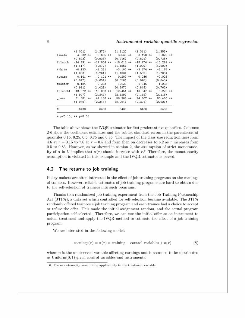
(1.001) (1.275) (1.312) (1.311) (1.353)female 4.632 ** 5.635 ** 3.546 ** 3.128 ** 3.025 **

(0.843) (0.933) (0.916) (0.821) (0.735)frlunch -14.491 ** -17.064 ** -16.618 ** -13.774 ** -10.291 **

(1.117) (1.272) (1.186) (1.099) (1.009)twhite -0.123 -1.251 -3.102 ** -3.674 ** -3.176 *

(1.083) (1.261) (1.403) (1.582) (1.703)tyears 0.141 ** 0.121 ** 0.209 ** 0.036 -0.025

(0.047) (0.054) (0.050) (0.048) (0.045)tmaster -0.184 0.333 1.230 1.346 1.233

(0.931) (1.028) (0.997) (0.845) (0.762)frlunchf -13.372 ** -15.053 ** -12.451 ** -10.347 ** -5.226 **

(1.947) (2.249) (2.329) (2.165) (2.118)_cons 31.581 ** 42.156 ** 56.903 ** 74.807 ** 80.450 **

(1.980) (2.314) (2.261) (2.301) (2.027)

N 6430 6430 6430 6430 6430

* p<0.10, ** p<0.05

The table above shows the IVQR estimates for first graders at five quantiles. Columns2-6 show the coefficient estimates and the robust standard errors in the parenthesis atquantiles 0.15, 0.25, 0.5, 0.75 and 0.85. The impact of the class size reduction rises from4.6 at τ = 0.15 to 7.6 at τ = 0.5 and from then on decreases to 6.2 as τ increases from0.5 to 0.85. However, as we showed in section 2, the assumption of strict monotonoc-ity of α in U implies that α(τ) should increase with τ .6 Therefore, the monotonocityassumption is violated in this example and the IVQR estimator is biased.

4.2 The returns to job training

Policy makers are often interested in the effect of job training programs on the earningsof trainees. However, reliable estimates of job training programs are hard to obtain dueto the self-selection of trainees into such programs.

Thanks to a randomized job training experiment from the Job Training PartnershipAct (JTPA), a data set which controlled for self-selection became available. The JTPArandomly offered trainees a job training program and each trainee had a choice to acceptor refuse the offer. This made the initial assignment random, and the actual programparticipation self-selected. Therefore, we can use the initial offer as an instrument toactual treatment and apply the IVQR method to estimate the effect of a job trainingprogram.

We are interested in the following model:

earnings(τ) = α(τ)× training + control variables + u(τ) (8)

where u is the unobserved variable affecting earnings and is assumed to be distributedas Uniform(0, 1) given control variables and instruments.

6. The monotonocity assumption applies only to the treatment variable.

D. Kwak 9

The data consist of 5, 102 observations for adult males on earnings, actual job train-ing, initial assignment status, and other individual characteristics. Earnings are mea-sured as total earnings over the 30-month period following the assignment into thetreatment or control group, and the mean and standard deviation of earnings in thesample are $19, 147 and $19, 540 respectively. The vector of control variables includesrace dummies, a dummy indicator of holding a high school diploma or GED, age dum-mies, a dummy for marital status, an indicator of availability of earnings data in thefollow-up survey, a dummy variable indicating whether a trainee worked 12 or moreweeks within a year prior to the assignment, and dummies for recommended strategiessuch as classroom training and on-the-job training.7

In Stata, we obtain the IVQR estimates with heteroskedasticity-robust standarderrors for equation (8) by typing:

. ivqreg earnings black hispanic married hs_GED workless13 age2225 ///> age2629 age3035 age3644 age4554 class_tr ojt_tr followup ///> (train_actual=train_offer) if sex==1, robust


Robustearnings Coef. Std. Err. t P>|t| [95% Conf. Interval]

train_actual 385.2386 963.0472 0.40 0.689 -1502.748 2273.226black -2116.101 651.5846 -3.25 0.001 -3393.487 -838.7145

hispanic 975.7167 1045.066 0.93 0.351 -1073.063 3024.496married 7734.16 804.9743 9.61 0.000 6156.064 9312.256hs_GED 3773.283 595.6394 6.33 0.000 2605.574 4940.993

workless13 -7674.56 646.5651 -11.87 0.000 -8942.106 -6407.014age2225 5192.876 1370.287 3.79 0.000 2506.524 7879.229age2629 5338.339 1417.867 3.77 0.000 2558.71 8117.969age3035 3632.297 1382.75 2.63 0.009 921.5121 6343.083age3644 2156.194 1392.201 1.55 0.122 -573.1196 4885.507age4554 1051.724 1468.433 0.72 0.474 -1827.037 3930.484

class_tr -925.41 805.8885 -1.15 0.251 -2505.298 654.4783ojt_tr 400.3772 698.6266 0.57 0.567 -969.2316 1769.986

followup 4226.798 689.1061 6.13 0.000 2875.854 5577.743_cons 7478.829 1553.25 4.81 0.000 4433.791 10523.87

The Stata output above shows the IVQR estimation results at 0.5 quantile of earningsfor adult males. The return of a training at 0.5 quantile is $385 and its standard erroris $963. A 95-percent confidence interval for the effect of a training at 0.5 quantileranges from -$1, 502 to $2, 272 thus the effect is not statistically significantly differentfrom zero. Below we again use estout to show the IVQR estimates of the returns to atraining program at various quantiles of earnings. The estimates imply that job trainingis not effective for those at low quantile of earnings. The effects of training at the 0.75and 0.85 quantiles are $2, 700 and $3, 131, respectively, and are statistically significant.

As α increases, the estimates for the impact of training increase from -$125 to $3, 131

7. See Abadie et al. (2002) for a detailed discussion of the variables and data. The data are takenfrom http://econ-www.mit.edu/faculty/angrist/data1/data/abangim02.


except at τ = 0.25. In particular, the effects of training at . Moreover, α is increasingin U , which is the distribution of earning after conditioning observed covariates, for thisexample.

Ordinary QR estimates with same data and the model in Chernozhukov and Hansen(2008) for the marginal effect of the job training are significantly different from zeroat all quantiles while the marginal effect of the job training from the IVQR method issignificant only for workers with earnings above 0.75 quantile.

.

. estout *, cells(b(star fmt(%7.0f)) se(par)) stats(N, fmt(%5.0f)) collabels(no> ne) sty(smcl) var(8) model(8) stard legend starlevels(* 0.10 ** 0.05)

tau15 tau25 tau5 tau75 tau85

train_~l -125 642 385 2617 * 3131 **(629) (700) (963) (1511) (1591)

black -38 -184 -2116 ** -3222 ** -2936 **(338) (398) (652) (1068) (1363)

hispanic 211 714 976 -497 603(538) (634) (1045) (1700) (1830)

married 504 2330 ** 7734 ** 10507 ** 10484 **(383) (481) (805) (1041) (1143)

hs_GED 482 1349 ** 3773 ** 6126 ** 6082 **(320) (381) (596) (992) (1191)

workl~13 -1073 ** -3202 ** -7675 ** -9691 ** -9936 **(317) (378) (647) (974) (1132)

age2225 1096 2399 ** 5193 ** 11490 ** 10371 **(791) (957) (1370) (1712) (3610)

age2629 1045 2165 ** 5338 ** 12806 ** 14536 **(801) (971) (1418) (1869) (3696)

age3035 754 1424 3632 ** 10977 ** 9788 **(782) (950) (1383) (1708) (3620)

age3644 348 189 2156 9345 ** 11257 **(769) (940) (1392) (1808) (3687)

age4554 226 120 1052 4829 ** 4596(827) (1011) (1468) (2138) (3906)

class_tr -93 352 -925 -2796 ** -2538(437) (512) (806) (1210) (1608)

ojt_tr -22 365 400 942 1348(348) (412) (699) (1037) (1203)

follow~y 419 1779 ** 4227 ** 984 282(363) (430) (689) (889) (1127)

_cons 242 1300 7479 ** 14177 ** 22516 **(887) (1050) (1553) (1930) (3611)

N 5102 5102 5102 5102 5102

* p<0.10, ** p<0.05

.

D. Kwak 11

5 Monte Carlo simulation

This section presents the finite sample properties of the IVQR estimator from section 2.We focus on two aspects of the IVQR estimator, the convergence of the estimator to thetrue value and the size of the test for H0 : α?(τ) = α(τ) in performing inference. Wealso report the mean of point estimates for the coefficients and for the standard errorsof the two-stage quantile regression and ordinary quantile regression for comparison.

5.1 Data generating process

The data generating process (DGP) for our simulation is given by

yi = α(τ)di + β1(τ)x1i + β2(τ)x2i + ui, i = 1, 2, .., n

For the sake of simplicity, we assume that the exogenous covariates have homoge-neous marginal effects which means that both β1(τ) and β2(τ) are constant.

q(d, x, τ) = α(τ)× d+ β1 × x1 + β2 × x2

All the exogenous variables are drawn from a standard normal density. The param-eter α is generated as

α(U) = f(U) (9)

where U ∼ Uniform(0, 1) and f is strictly increasing in U and it satisfies the mainconditions for identification given by

P [Y ≤ q(d,x, τ)|Z,X] = τ (10)

The DGP for the variables is given by


X1iid∼ N(0, 1)

X2iid∼ N(0, 1)

Zjiid∼ N(0, 1), j = 1, 2

Uiid∼ N(0, 1)

V =U

2+W

4, W

iid∼ N(0, 1)

D0 = 1× (X2

2+Z1

2+V

2> 0)

D1 = 1× (X2

2+Z1 + Z2

2+V

2> 0)

Y = α(τ)Di + β1 ×X1 + β2 ×X2 + U

where i = 0, 1, β1 = 0, β2 = 1, α(U, τ) = τth percentile value of ϕ(U), ϕ is a standardnormal cdf for the normal error term, and ϕ is an identity function for the uniformerror, ϕ(U)=U . The endogeneity problem occurs through V that induces the correlationbetween U and Di. D0 is used in exactly-identified case and D1 is used in over-identifiedcase.

All simulation results presented in this section are based on 2000 replications withthe number of observations of 200, 500, 1000, and 2000. We provide simulation resultswith the number of observations of 5000 at the tails of distribution, since the speed ofconvergence is slow at the tails. 8

5.2 Convergence of estimator

This section shows the Monte Carlo (MC) simulation results for the convergence of thecoefficient estimates and the size of test. Tables 2 and 3 report the simulation resultswith a normal error and Tables 4 and 5 report the simulation results with a uniformerror. The Mean(α(τ)) column reports the mean of the IVQR estimates for α(τ). TheSD column reports the standard deviation of the coefficient estimates for α(τ) while theMean(σα(τ))) column reports the mean of heteroskedasticity-robust standard errors for

α(τ). The MeanSD column reports the ratio of the mean of the standard errors estimates

for α(τ) to the standard deviation of the coefficient estimates for α(τ). The Mean(r)column reports the mean of the estimates for the rejection rate of the null hypothesisH0 : α?(τ) = α(τ) at the .05 level. Finally, the last two columns report a 95-percentconfidence interval for the mean of the rejection rate, r.

Table 2 shows the results for a just-identified case and table 3 shows the results for anover-identified case. The second column of table 2 reports the mean of point estimates

8. A simple back-of-the-envelope rule of thumb would be that in a sample size of, say 1000 whenlooking at the 10th or 90th percentile, the behavior will be much closer to the behavior of a measureof central tendency based on say 100-200 observations.

D. Kwak 13

for α(τ). A consistent estimator for α(τ) should converge to τ as n increases since α(τ)is U for a uniform error and is cdf(U) for a normal error. The second column of table 2shows that the mean estimates for α(τ) converge to the true value of α(τ) as n increases.The convergence to true values of the parameters occurs across the whole distributionof the dependent variable. The second column of table 3 reports the mean of pointestimates for α(τ) for an over-identified case. The mean estimates for α(τ) converge tothe true value of α(τ) as n increases across all quantiles of the dependent variable. Theconvergence is slower at tails of the distribution such as τ=0.1 and τ=0.9. However,eventually for large enough n, the mean of the point estimates for α(τ) converges to thetrue value across all quantiles of the dependent variable.

5.3 The size of the test

We study the coverage of the coefficient estimates for the endogenous variable for theIVQR estimator by examining the estimates for the rejection rate and the ratio of themean of the MC estimates of the standard error for α(τ) to the standard deviation ofα(τ). To test the size of the hypothesis, we define the rejection rate, r, as an indicatorof the rejection for the null hypothesis, H0 : α?(τ) = α(τ):

r ≡ 1× (α(τ)− αtrue(τ)

σα(τ)> CV.05)

where CV.05 is the critical value from a t-table.

Columns 6-8 report the mean of the MC estimates for the rejection rate, r, andtheir 95 percent confidence interval (CI). For instance, table 2 reports the results for ajust-identified case with a normal error. Except for the cases of τ=0.1 and τ=0.9, the 95percent CIs of the rejection rate contains the true rejection rate. Even for the cases ofτ=0.1 and τ=0.9, as n increases over 500, the 95 percent CIs contain the true rejectionrate of 0.05. The simulation results show that the size distortion does not appear at thecenter of the distribution and it disappears at the tails of the distribution as n exceeds500. This implies that the precise inference at the tails of the distribution requires moreobservations than at the center of distribution.

Table 3 reports the estimation results from the simulations for an over-identifiedcase with a normal error. Columns 6-8 show that the 95 percent CIs of the rejectionrate contains the true value of .05 for all the samples and for the quantiles 0.25-0.75. Atthe tails of the distribution where τ is 0.1 and 0.9, the 95 percent CIs of the rejectionrate contain the true level of .05 when the number of observations exceeds 500.

In summary, for both the exactly-identified and over-identified case, when the errorprocess is drawn from a normal distribution, the IVQR estimator provides the correctinference across all quantiles as n increases. However, the sample size should be greaterthan 500 if we wish to perform a precise inference at the tails of the distribution of thedependent variable.


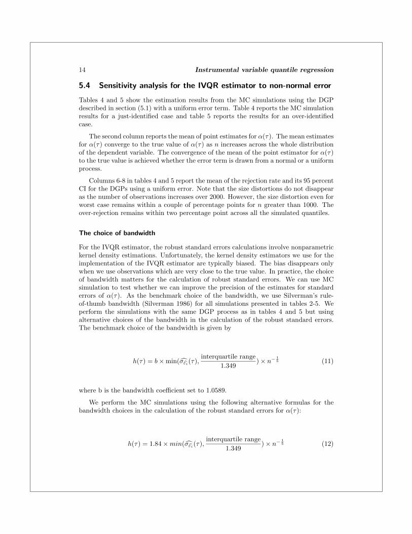
5.4 Sensitivity analysis for the IVQR estimator to non-normal error

Tables 4 and 5 show the estimation results from the MC simulations using the DGPdescribed in section (5.1) with a uniform error term. Table 4 reports the MC simulationresults for a just-identified case and table 5 reports the results for an over-identifiedcase.

The second column reports the mean of point estimates for α(τ). The mean estimatesfor α(τ) converge to the true value of α(τ) as n increases across the whole distributionof the dependent variable. The convergence of the mean of the point estimator for α(τ)to the true value is achieved whether the error term is drawn from a normal or a uniformprocess.

Columns 6-8 in tables 4 and 5 report the mean of the rejection rate and its 95 percentCI for the DGPs using a uniform error. Note that the size distortions do not disappearas the number of observations increases over 2000. However, the size distortion even forworst case remains within a couple of percentage points for n greater than 1000. Theover-rejection remains within two percentage point across all the simulated quantiles.

The choice of bandwidth

For the IVQR estimator, the robust standard errors calculations involve nonparametrickernel density estimations. Unfortunately, the kernel density estimators we use for theimplementation of the IVQR estimator are typically biased. The bias disappears onlywhen we use observations which are very close to the true value. In practice, the choiceof bandwidth matters for the calculation of robust standard errors. We can use MCsimulation to test whether we can improve the precision of the estimates for standarderrors of α(τ). As the benchmark choice of the bandwidth, we use Silverman’s rule-of-thumb bandwidth (Silverman 1986) for all simulations presented in tables 2-5. Weperform the simulations with the same DGP process as in tables 4 and 5 but usingalternative choices of the bandwidth in the calculation of the robust standard errors.The benchmark choice of the bandwidth is given by

h(τ) = b×min(σεi(τ),interquartile range

1.349)× n− 1

5 (11)

where b is the bandwidth coefficient set to 1.0589.

We perform the MC simulations using the following alternative formulas for thebandwidth choices in the calculation of the robust standard errors for α(τ):

h(τ) = 1.84×min(σεi(τ),interquartile range

1.349)× n− 1

5 (12)

D. Kwak 15

and

h(τ) = 1.0589×min(σεi(τ),interquartile range

1.349)× n− 1

3 (13)

The bandwidth in (12) is larger than Silverman’s bandwidth and the bandwidth in(13) is smaller than Silverman’s bandwidth.9

Standard error calculation with the alternative bandwidth choices

Using the DGP with a uniform error, we perform two additional sets of simulationswith alternative bandwidth choices given in (12) and (13) for the just-identified andover-identified case.

In both cases, the mean estimates for α(τ) converge to the true value of α(τ) forthe whole distribution of the dependent variable as n increases. However, the sizedistortions do not disappear for either bandwidth. The results imply that we cannotobtain an optimal bandwidth that provides the correct size of tests across all quantilesfor a uniform error. The IVQR estimator is not robust to the error process from auniform distribution.

5.5 Two stage quantile regression and ordinary quantile regression

Tables 6 and 7 show two-stage quantile regression estimates and ordinary quantile re-gression estimates, respectively, using the variables generated from the DGP in section(5.1). The results show that the parameter estimates are biased and the bias does notdisappear with an increase in sample size. The results in tables 6 and 7 imply that theIVQR method can deliver unbiased estimates whereas the two-stage QR and ordinaryQR fail to obtain unbiased estimates.

5.6 Sensitivity of the IVQR estimator to weak or irrelevant IVs

The IVQR method implemented in this article requires strong instruments for preciseinference. The model in section 2 suggests that the quality of asymptotic approximationdiminishes rather quickly when the instruments are weak or irrelevant. Chernozhukovand Hansen (2008) propose a dual inference method which is robust to weaker or ir-relevant IVs. This method is based on the Wald statistic which can be constructedfrom the test of the null hypothesis that the coefficients of the instruments are zero.When α?(τ) = α(τ), this statistic is asymptotically chi-squared with dim(z) degrees offreedom. Therefore, a valid confidence region for α(τ) can be obtained based on the

9. The choice of the bandwidth coefficient of 1.84 is based on the upper bound calculation for a uniformkernel density estimation; see Salgado-Ugarte et al. (1995). In our specification, the bandwidthcoefficient has an upper bound of 2.27.


inversion of this dual Wald statistic.10

10. See Chernozhukov and Hansen (2008, p.383) for more details. We leave the implementation of thismethod and the examination of its finite sample properties for future research.

D. Kwak 17

DGP with a normal error processes

[Table 2] Endogenous treatment effect for just-identified case

τ = 0.1 Mean (α(τ)) SD (α(τ)) Mean(σα(τ))Mean(σα(τ))

SD(α(τ)) Mean(r) 95% CI of r

n=200 0.076 0.602 0.583 0.968 0.061 (0.051,0.071)n=500 0.085 0.339 0.331 0.976 0.049 (0.039,0.059)n=1000 0.096 0.242 0.233 0.963 0.056 (0.046,0.066)n=2000 0.098 0.170 0.164 0.959 0.065 (0.055,0.075)n=5000 0.099 0.105 0.104 0.981 0.057 (0.047,0.067)



n=200 0.241 0.424 0.431 1.016 0.045 (0.035,0.055)n=500 0.246 0.267 0.268 1.004 0.048 (0.038,0.057)n=1000 0.246 0.190 0.188 0.989 0.058 (0.048,0.068)n=2000 0.248 0.130 0.131 1.015 0.054 (0.044,0.064)



n=200 0.502 0.394 0.395 1.003 0.049 (0.039,0.058)n=500 0.494 0.246 0.246 1.001 0.050 (0.040,0.060)n=1000 0.494 0.171 0.172 1.006 0.050 (0.040,0.060)n=2000 0.501 0.122 0.121 0.992 0.055 (0.045,0.065)



n=200 0.723 0.407 0.421 0.995 0.047 (0.036,0.055)n=500 0.748 0.261 0.259 1.034 0.051 (0.040,0.060)n=1000 0.743 0.182 0.181 0.992 0.054 (0.044,0.066)n=2000 0.749 0.128 0.127 0.977 0.051 (0.041,0.061)



n=200 0.838 0.567 1.610 2.839 0.065 (0.054,0.076)n=500 0.869 0.339 0.318 0.938 0.067 (0.057,0.077)n=1000 0.892 0.234 0.224 0.957 0.067 (0.057,0.077)n=2000 0.897 0.161 0.158 0.981 0.055 (0.045,0.065)n=5000 0.898 0.101 0.100 0.990 0.058 (0.048,0.068)


[Table 3] Endogenous treatment effect for over-identified case



n=200 0.077 0.520 0.455 0.875 0.078 (0.051,0.071)n=500 0.082 0.303 0.278 0.917 0.056 (0.046,0.067)n=1000 0.093 0.213 0.197 0.925 0.060 (0.050,0.070)n=2000 0.103 0.139 0.139 1.008 0.048 (0.037,0.058)n=5000 0.100 0.089 0.088 0.978 0.055 (0.045,0.065)



n=200 0.245 0.388 0.373 0.961 0.058 (0.047,0.068)n=500 0.248 0.240 0.232 0.967 0.059 (0.049,0.068)n=1000 0.250 0.168 0.164 0.970 0.054 (0.044,0.064)n=2000 0.250 0.116 0.115 0.975 0.055 (0.045,0.065)



n=200 0.496 0.358 0.345 0.964 0.065 (0.054,0.075)n=500 0.496 0.225 0.217 0.964 0.056 (0.046,0.066)n=1000 0.500 0.152 0.152 0.997 0.054 (0.044,0.064)n=2000 0.500 0.106 0.107 1.009 0.047 (0.037,0.056)



n=200 0.717 0.423 0.423 1.000 0.050 (0.039,0.059)n=500 0.737 0.267 0.267 1.002 0.048 (0.038,0.057)n=1000 0.750 0.159 0.158 0.994 0.055 (0.045,0.066)n=2000 0.750 0.112 0.111 0.994 0.055 (0.045,0.065)



n=200 0.830 0.582 0.837 1.438 0.062 (0.051,0.072)n=500 0.865 0.339 0.330 0.973 0.059 (0.049,0.069)n=1000 0.895 0.199 0.189 0.950 0.067 (0.057,0.077)n=2000 0.900 0.142 0.134 0.944 0.055 (0.045,0.065)n=5000 0.900 0.087 0.085 0.977 0.059 (0.049,0.069)

D. Kwak 19

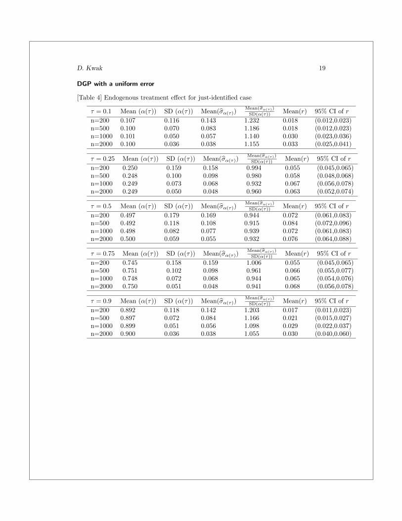
DGP with a uniform error

[Table 4] Endogenous treatment effect for just-identified case



n=200 0.107 0.116 0.143 1.232 0.018 (0.012,0.023)n=500 0.100 0.070 0.083 1.186 0.018 (0.012,0.023)n=1000 0.101 0.050 0.057 1.140 0.030 (0.023,0.036)n=2000 0.100 0.036 0.038 1.155 0.033 (0.025,0.041)



n=200 0.250 0.159 0.158 0.994 0.055 (0.045,0.065)n=500 0.248 0.100 0.098 0.980 0.058 (0.048,0.068)n=1000 0.249 0.073 0.068 0.932 0.067 (0.056,0.078)n=2000 0.249 0.050 0.048 0.960 0.063 (0.052,0.074)



n=200 0.497 0.179 0.169 0.944 0.072 (0.061,0.083)n=500 0.492 0.118 0.108 0.915 0.084 (0.072,0.096)n=1000 0.498 0.082 0.077 0.939 0.072 (0.061,0.083)n=2000 0.500 0.059 0.055 0.932 0.076 (0.064,0.088)



n=200 0.745 0.158 0.159 1.006 0.055 (0.045,0.065)n=500 0.751 0.102 0.098 0.961 0.066 (0.055,0.077)n=1000 0.748 0.072 0.068 0.944 0.065 (0.054,0.076)n=2000 0.750 0.051 0.048 0.941 0.068 (0.056,0.078)



n=200 0.892 0.118 0.142 1.203 0.017 (0.011,0.023)n=500 0.897 0.072 0.084 1.166 0.021 (0.015,0.027)n=1000 0.899 0.051 0.056 1.098 0.029 (0.022,0.037)n=2000 0.900 0.036 0.038 1.055 0.030 (0.040,0.060)


[Table 5] Endogenous treatment effect for over-identified case



n=200 0.103 0.107 0.126 1.178 0.024 (0.017,0.030)n=500 0.099 0.064 0.074 1.156 0.020 (0.014,0.026)n=1000 0.099 0.047 0.051 1.085 0.032 (0.024,0.039)n=2000 0.098 0.033 0.034 1.030 0.041 (0.032,0.050)



n=200 0.249 0.148 0.144 0.973 0.064 (0.053,0.074)n=500 0.250 0.093 0.090 0.968 0.064 (0.053,0.075)n=1000 0.250 0.066 0.063 0.955 0.055 (0.045,0.065)n=2000 0.249 0.046 0.045 0.978 0.060 (0.049,0.070)



n=200 0.500 0.173 0.156 0.902 0.090 (0.077,0.102)n=500 0.498 0.110 0.101 0.918 0.084 (0.072,0.096)n=1000 0.500 0.074 0.072 0.973 0.062 (0.051,0.073)n=2000 0.500 0.051 0.051 0.992 0.055 (0.045,0.065)



n=200 0.751 0.147 0.144 0.980 0.067 (0.056,0.078)n=500 0.748 0.092 0.089 0.967 0.062 (0.051,0.072)n=1000 0.750 0.064 0.063 0.984 0.057 (0.047,0.067)n=2000 0.751 0.046 0.044 0.956 0.060 (0.050,0.070)



n=200 0.897 0.108 0.126 1.166 0.014 (0.009,0.019)n=500 0.897 0.065 0.074 1.138 0.020 (0.013,0.026)n=1000 0.901 0.044 0.050 1.136 0.027 (0.020,0.034)n=2000 0.900 0.032 0.034 1.062 0.035 (0.026,0.043)

D. Kwak 21

[table 6] Two-stage QR for over-identified case


SD(α(τ))

n=200 0.108 0.113 0.102 0.903n=500 0.101 0.064 0.062 0.954n=1000 0.102 0.046 0.043 0.935n=2000 0.102 0.026 0.025 0.962


SD(α(τ))

n=200 0.255 0.151 0.155 1.104n=500 0.254 0.093 0.095 1.074n=1000 0.262 0.068 0.067 1.030n=2000 0.259 0.038 0.038 1.008


SD(α(τ))

n=200 0.513 0.169 0.199 1.178n=500 0.518 0.110 0.120 1.091n=1000 0.527 0.077 0.084 1.091n=2000 0.525 0.045 0.048 1.067


SD(α(τ))

n=200 0.762 0.152 0.206 1.365n=500 0.774 0.103 0.127 1.233n=1000 0.775 0.067 0.086 1.283n=2000 0.778 0.041 0.050 1.220


SD(α(τ))

n=200 0.763 0.220 0.191 0.868n=500 0.785 0.136 0.116 0.853n=1000 0.780 0.093 0.081 0.871n=2000 0.789 0.053 0.047 0.887


[table 7] Ordinary QR for over-identified case


SD(α(τ))

n=200 0.172 0.078 0.079 1.013n=500 0.169 0.046 0.042 0.913n=1000 0.170 0.034 0.029 0.853n=2000 0.170 0.019 0.016 0.842


SD(α(τ))

n=200 0.384 0.107 0.098 0.916n=500 0.389 0.062 0.060 0.968n=1000 0.394 0.046 0.042 0.913n=2000 0.391 0.027 0.024 0.889


SD(α(τ))

n=200 0.676 0.114 0.119 1.044n=500 0.679 0.071 0.072 1.014n=1000 0.686 0.051 0.051 1.006n=2000 0.688 0.030 0.029 0.973


SD(α(τ))

n=200 0.884 0.099 0.107 1.080n=500 0.892 0.062 0.066 1.064n=1000 0.891 0.043 0.045 1.047n=2000 0.894 0.025 0.026 1.040


SD(α(τ))

n=200 0.967 0.074 0.079 1.067n=500 0.970 0.045 0.047 1.044n=1000 0.970 0.031 0.032 1.032n=2000 0.972 0.018 0.019 1.056

D. Kwak 23

6 Methods and formulas

In this section, we provide the formulas for the IVQR estimator for θ(τ) and its standarderror. The formulas for the parameters and standard errors in Chernozhukov and Hansen(2006) are used for the just-identified case and the formulas in Chernozhukov and Hansen(2008) are used for the over-identified case.

6.1 Coefficient parameter

Given τ , the objective function we use in implementation is:

Qn(τ, α, β, γ) =1

n

n∑i=1

ρτ [yi − d′iα(τ) + x′iβ(τ)−£′iγ]Vi (14)

where ρτ (u) = (τ − 1[u < 0])× u, £i = f(zi,xi) is a dim(γ)-vector of IVs such thatdim(γ) ≥dim(α), and Vi = V(zi,xi) is scalar weight. We obtain parameter estimatesby minimizing Qn(τ, α, β, γ). In the actual implementation, we set Vi = 1 and £i = zifor simplicity.

For a given value of τ and given the structural parameter α(τ), applying an ordinary

quantile regression of yi − d′iα(τ) on (z′i,x′i) delivers the estimator ϑ given by

ϑ(α(τ)) ≡ (γ(α(τ)), β(α(τ)) = arg minγ,β

Qn(α(τ), γ, β)

For a given value of τ , we do a grid search for α(τ) by finding α(τ) that makesγ(α, τ) as close to zero as possible:

α(τ) = arg infα(τ),α∈Λ

[γ(α(τ), τ)′]× An(α(τ))× [γ(α(τ), τ)] (15)

where A(α) is a positive definite weighting matrix and the inverse of covariancematrix for γ(α, τ).

We obtain the IVQR estimate, θ(τ), by applying an ordinary quantile regression ofyi − d′iα(τ) to (z′i,x

′i):

θ(τ) = (α(τ)′, β(α(τ))′)


6.2 Standard errors

Using equation (14) as the objective function, we can perform inference based on GMM.

We obtain heteroskedasticity robust standard errors for θ(τ) from equation (16):11

√n(θ(τ)− θ(τ))→d N(0,Ωθ), Ωθ = (R′ L′)′S(R′ L′) (16)

where

σ(θ(τ)) =

√diag[Cov(θ(τ))]

Cov(θ(τ)) =1

nΩθ(τ)

S = τ(1− τ)E(ΨiΨ′i)

Ψi = [z′ix′i]

R = (J ′αHJα)−1J ′αH

H = J′γA(α(τ))Jγ

L = JβM

M = Ik+r − J ′αRJα = E[fε(0|x, z,D)ΨD′]

Jϑ = E[fε(0|x, z)ΨΨ′/V]

J−1ϑ =

[JγJβ

]εi = Yi −D′iα(τ)− x′iβ(τ)

Standard error for just-identified case

When dim(z) = dim(d), the choice of the weighting matrix A(α(τ)) does not affect theasymptotic variance. Therefore, with the just-identified instruments, the asymptoticvariance of θ(τ) has a simpler form:

Ωθ = J−1θ S(J ′θ)

−1

Jθ = E[fε(0|x, z,D)Ψ]× [D′,x′]

S = τ(1− τ)E(ΨiΨ′i)

11. This is based on the asymptotic analysis in Chernozhukov and Hansen (2008, p.384–387).

D. Kwak 25

6.3 IVQR agorithm for just-identified case

For given each quantile τ , the IVQR method starts with constructing the set of gridpoints using two-stage quantile regression estimates for α(τ) and its standard error.

1. Step 1: (Construction of the set of grid points for α(τ)) Run a linear projection ofd1 on x′ and z1. And obtain its predicted value and denote it as £i = [z1i x′]π.Using £i, for given τ , perform an ordinary QR of y on £ix

′. Keep the coefficientestimate for £i and the residuals ei. Using the residuals, obtain σ0(τ) using

σ0(τ) =τ(1− τ)

φ∗(Φ∗−1(τ))2

( n∑i=1

ΨiΨ′i

)(17)

where Ψi = [£′iX′i]′, φ∗ is a standardized normal pdf, and Φ∗ is a standardized

normal cdf. Use the initial estimates of the coefficient for zi and the standarddeviation for σ0 to construct a set of grid points.12 Denote the initial coefficientestimate and the standard deviation as α0(τ) and σ0(τ), respectively.

2. Step 2: (Construction of the set of grid search points) The lower and upper boundfor the set of grid search points is defined as α0(τ)−2∗ σ0(τ) and α0(τ)+2∗ σ0(τ),

respectively. Use σ0(τ)S as a step size in the grid search. The default behavior of

ivqreg is to use S = 20. Thus, the default set of the grid search points for α(τ)is:

G(τ) = α0(τ)− 2σ0(τ), α0(τ)− 2σ0(τ) +σ0(τ)

20, . . . , α0(τ) + 2σ0(τ)

= α1(τ), α2(τ), . . . , αj(τ), . . . , α80(τ)

where j = 1, 2, 3, ...80.

3. Step 3: Using the set of grid points from step 2, run a series of ordinary quantileregressions. Apply a series for ordinary QR of y − αj(τ)× d on (z,x).13

yi − di × αj(τ) = zi × γj(τ) + x′i × βj(τ) + εi2

Keep the coefficient and the inverse of covariance matrix for zi and denote themas γj(τ) and A(τ), respectively The optimal α(τ) is obtained by minimizing thedistance of γj(τ) given by

||γj(τ)|| = γj(τ)′A(τ)γj(τ)

12. The initial estimates are based on an extension of 2SLAD in Amemiya (1982) to two-stage QR.13. In Stata, this is equivalent to running qreg on y − αj(τ) × d on z,x, q(τ) for each j.


We obtain the optimal α(τ) from

α(τ) = arg minαj(τ)

γj(αj(τ), τ)′A(αj(τ), τ)γj(αj(τ), τ) (18)

4. Step 4: Obtain the IVQR estimator by running an ordinary QR of y − α(τ) × don (z,x). Obtain ϑ(τ) from the coefficient estimates for (z,x) and denote them

as γ(α(τ), τ), β(α(τ), τ), respectively. Finally, obtain the IVQR estimator θ(τ) =

[α(τ), β(α(τ), τ)′]′.

5. Step 5 (Standard error) Standard error calculation is given by

Ωθ = J−1θ SJ ′θ

−1

S = τ(1− τ)E(ΨΨ′)

Jθ = E[fε(0|x, z,d)× Z× [d,x]′]

Z = [z,x]

The kernel density estimation for εi(τ) is based on Powell (1986) and Koenker(2005):

Jθ = E[fε(0|x, z,d)× Z× [d,x′]]

Jθ(τ) =1

n

n∑i=1

K( εi(τ)h(τ) )

h(τ)× Zi × [di, x′i]

where εi(τ) is given as

εi(τ) = yi − diα(τ)− x′iβ(α(τ), τ)

where K(·) = φ(·) of the Gaussian kernel density and h(τ) = 1.364× (2√π)−

15 ×

σεi(τ)× n− 15 is the bandwidth proposed by Silverman (1986).

And we estimate S = τ(1− τ)E(ΨΨ′) by

S(τ) = τ(1− τ)1

n

n∑i=1

(ZiZ′i)

Finally, we obtain

V (θ(τ)) from

V (θ(τ)) =

1

nJθ(τ)−1S(τ)(Jθ(τ)′)−1 (19)

We obtain the standard errors of θ(τ), denoted σ(θ(τ)), by taking the square root

of the diagonal elements of

V (θ(τ)).

D. Kwak 27

6.4 IVQR algorithm for over-identified case

The algorithm for the over-identified case is based on the formulas in Chernozhukov andHansen (2008). Steps 1 and 2 are are the same as in the just-identified case. Then weproceed with minimizing the distance of γ(τ), ||γ(τ)||. Let z = z1, z2, . . . , zr.

1. Step 3: (Minimize the distance ||γ(τ)||) Run a series of ordinary quantile regressionof y − αj(τ)× d on (z,x):14

yi − di × αj(τ) = z′i × γj(τ) + x′i × βj(τ) + εi2

Keep the coefficient vector on zi, γj(τ) and the residual εj2, to construct the weightA(τ) for the calculation of the distance of ||γj(τ)||. The optimal α(τ) is obtainedby minimizing ||γj(τ)||:

εj2(τ) = yi − di × αj(τ)− z′i × γj(τ)− x′i × βj(τ)

Jθj

(τ) =1

nh(τ)

n∑i=1

φ(εj2ih(τ)

)× ZiZ′i

S(τ) = τ(1− τ)1

n

n∑i=1

ZiZ′i

Jαj

(τ) =1

nh(τ)

n∑i=1

φ(εj2ih(τ)

)× diZ′i

Zi = [z′i,x′i]′

Ξ(τ) = Jθj

(τ)−1 =

[Jγj (τ)

Jβj (τ)

]

where h(τ) is the same as in the just-identified case.

A(αj(τ), τ) = [Jγj (τ)S(τ)(Jγj (τ))′]−1

||γj(τ)|| = γj(τ)′A(αj(τ), τ)γj(τ)

α(τ) = arg minαj(τ),j=1,2,..,J

γj(αj(τ), τ)′A(αj(τ), τ)γj(αj(τ), τ)

2. Step 4: Using the optimal α(τ) obtained in step 3, use qreg to calculate y−d×α(τ)on (z,x, q(τ)).

yi − diα(τ) = z′iγ(τ) + x′iβ(τ) + ε2i

14. In Stata, one can use qreg to calculate y − αj(τ) × d on z,x, q(τ).


Keep the coefficients γ(α(τ), τ) and β(α(τ), τ) and denote ϑ(τ) = (γ(α(τ), τ)′, β(α(τ), τ)′)′

and θ(τ) = (α(τ), β(α(τ), τ)′)′.

3. Step 5: Calculate heteroskedasticity-robust standard errors.

Ωθ = (R′L′)′S(R′L′)

S = τ(1− τ)E(ZiZ′i)

R = (J ′αHJα)−1J ′αH

H = J′γA(α(τ))Jγ

L = JβM

M = Ik+r − J ′αR

Following Chernozhukov and Hansen (2008), we suggest a feasible standard errorestimator which is function of both observed data and bandwidth choice as below.

S(τ) = τ(1− τ)1

n

n∑i=1

ZiZ′i

εi(τ) = yi − diα(τ)− x′iβ(α(τ), τ)− z′iγ(α(τ), τ)

Jα(τ) =1

n

n∑i=1

K( εi(τ)h(τ) )

h(τ)× diZ

′i

Ξ(τ) =1

n

n∑i=1

K( εi(τ)h(τ) )

h(τ)ZiZ

′i[

Jγ(τ)

Jβ(τ)

]= Ξ(τ)−1; Jγ(τ), Jβ(τ)

H(τ) = J′γ(τ)× A(α(τ))× Jγ(τ)

A(α(τ)) = [Jγ(τ)S(τ)J′γ(τ)]−1

R(τ) = [Jα(τ)H(τ)Jα(τ)′]−1Jα(τ)H(τ)

L(τ) = Jβ(τ)− Jβ(τ)J ′αR(τ)

Finally, we obtain

V (θ(τ)).

V (θ(τ)) =

1

nΩθ(τ) =

1

n(R(τ)′L(τ)′)′S(τ)(R(τ)′L(τ)′)

We obtain the robust standard errors of θ(τ) by taking the square-root of the

diagonal elements of

V (θ(τ)).

D. Kwak 29

7 Saved results

ivqreg saves the following information in e():

Scalarse(N) number of observations e(df m) model degrees of freedome(df r) residual degrees of freedom e(q) quantile requestede(L) number of instruments e(M) number of endogenous variablese(rank) rank of e(V) e(grid) number of grid pointse(bwidth) bandwidth coefficient

Macrose(cmd) ivqreg e(cmdline) command as typede(title) title in estimation output e(depvar) name of dependent variablee(endo) name of endogenous variables e(exog) names of exogenous variablese(instr) names of excluded instruments e(properties) b V

Matricese(b) coefficient vector of the IVQR e(V) variance-covariance matrix of

estimator the IVQR estimatore(b 2sls) coefficient vector of the TSLS e(V 2sls) variance-covariance matrix of

estimator the TSLS estimator

Functionse(sample) marks estimation sample

8 Conclusion

In this article we introduced the ivqreg command for quantile regression with en-dogenous treatment variables. We demonstrated, using simulation with endogenoustreatment variables, that the IVQR estimator produces a consistent estimate while thetwo-stage quantile regression estimator fails to produce a consistent estimate at cer-tain percentiles. We also showed, using the DGP with normal errors, that the robustinference with the IVQR method was quite successful.

9 ReferencesAbadie, A., J. Angrist, and G. Imbens. 2002. Instrumental Variables estimates of the

effect of subsidized traning on the quantiles of traninee earnings. Econometrica 70:91–117.

Abrevaya, J., and C. M. Dahl. 2008. The effects of birth inputs on birthweight: Evidencefrom quantile estimation on panel data. Journal of Business and Economic Statistics26: 379–397.

Amemiya, T. 1982. Two stage least absolute diviation estimator. Econometrica 50:689–712.

Card, D. 1996. The effect of unions on the structure of wages: A logitudinal analysis.Econometrica 64: 957–980.

Chernozhukov, V., and C. Hansen. 2004. The Impact of 401(k) Participation on the


Wealth Distribution: An Instrumental Quantile Regression Analysis. Review of Eco-nomics and Statistics 86: 735–751.

———. 2005. An IV model of quantile treatment effects. Econometrica 73: 245–261.

———. 2006. Instrumental quantile regression inference for structural and treatmenteffect models. Journal of Econometrics 132: 491–525.

———. 2008. Instrumental variable quantile regression: A robust inference approach.Journal of Econometrics 142: 379–398.

Chernozhukov, V., C. Hansen, and M. Jansson. 2007. Inference approaches for instru-mental variable quantile regression. Economics letters 95: 272–277.

Chesher, A. 2003. Identification in nonseparable model. Econometrica 73: 1525–1550.

Imbens, G., and W. Newey. 2009. Identification and estimation of triangular simulta-neous equations model without additivity. Econometrica 77: 1481–1511.

Jann, B. 2005. Making regression tables from stored estimates. The Stata Journal 5(3):288–308.

———. 2007. Making regression tables simplified. The Stata Journal 7(2): 227–244.

Koenker, R. 2005. Quantile Regression. New York: Cambridge University Press.

Koenker, R., and G. Bassett. 1978. Regression quantiles. Econometrica 46: 33–50.

Koenker, R., and S. Portnoy. 1987. L-estimation for linear models. Journal of AmericanStatistical Association 82: 851–857.

Krueger, A. B. 1999. Experimental estimates of education production functions. Quar-terly Journal of Economics 114: 497–532.

Lee, S. 2007. Endogeneity in quantile regression models: A control function approach.Journal of Econometrics 141: 1131–1158.

Powell, J. 1986. Censored regression quantiles. Journal of Econometrics 23: 143–155.

Salgado-Ugarte, I. H., M. Shimuzu, and T. Taniuchi. 1995. snp6.2: practical rules forbandwidth selection in univariate density estimation. Stata Technical Bulletin 27:5–19.

Silverman, B. W. 1986. Density Estimation. London: Chapman and Hall.

The Stata Journal ( Instrumental variable quantile regression method …kwakdo/ivqreg.pdf · The Stata Journal (yyyy) vv, Number ii, pp. 1{30 Instrumental variable quantile regression

Documents