Roßbach, Peter; Karlow, Denis Working Paper The stability of traditional measures of index tracking quality Frankfurt School - Working Paper Series, No. 164 Provided in Cooperation with: Frankfurt School of Finance and Management Suggested Citation: Roßbach, Peter; Karlow, Denis (2011) : The stability of traditional measures of index tracking quality, Frankfurt School - Working Paper Series, No. 164, Frankfurt School of Finance & Management, Frankfurt a. M. This Version is available at: http://hdl.handle.net/10419/45496 Standard-Nutzungsbedingungen: Die Dokumente auf EconStor dürfen zu eigenen wissenschaftlichen Zwecken und zum Privatgebrauch gespeichert und kopiert werden. Sie dürfen die Dokumente nicht für öffentliche oder kommerzielle Zwecke vervielfältigen, öffentlich ausstellen, öffentlich zugänglich machen, vertreiben oder anderweitig nutzen. Sofern die Verfasser die Dokumente unter Open-Content-Lizenzen (insbesondere CC-Lizenzen) zur Verfügung gestellt haben sollten, gelten abweichend von diesen Nutzungsbedingungen die in der dort genannten Lizenz gewährten Nutzungsrechte. Terms of use: Documents in EconStor may be saved and copied for your personal and scholarly purposes. You are not to copy documents for public or commercial purposes, to exhibit the documents publicly, to make them publicly available on the internet, or to distribute or otherwise use the documents in public. If the documents have been made available under an Open Content Licence (especially Creative Commons Licences), you may exercise further usage rights as specified in the indicated licence.

Welcome message from author
This document is posted to help you gain knowledge. Please leave a comment to let me know what you think about it! Share it to your friends and learn new things together.
Transcript
Roßbach, Peter; Karlow, Denis
Working Paper
The stability of traditional measures of index trackingquality
Frankfurt School - Working Paper Series, No. 164
Provided in Cooperation with:Frankfurt School of Finance and Management
Suggested Citation: Roßbach, Peter; Karlow, Denis (2011) : The stability of traditional measuresof index tracking quality, Frankfurt School - Working Paper Series, No. 164, Frankfurt School ofFinance & Management, Frankfurt a. M.
This Version is available at:http://hdl.handle.net/10419/45496
Standard-Nutzungsbedingungen:
Die Dokumente auf EconStor dürfen zu eigenen wissenschaftlichenZwecken und zum Privatgebrauch gespeichert und kopiert werden.
Sie dürfen die Dokumente nicht für öffentliche oder kommerzielleZwecke vervielfältigen, öffentlich ausstellen, öffentlich zugänglichmachen, vertreiben oder anderweitig nutzen.
Sofern die Verfasser die Dokumente unter Open-Content-Lizenzen(insbesondere CC-Lizenzen) zur Verfügung gestellt haben sollten,gelten abweichend von diesen Nutzungsbedingungen die in der dortgenannten Lizenz gewährten Nutzungsrechte.
Terms of use:
Documents in EconStor may be saved and copied for yourpersonal and scholarly purposes.
You are not to copy documents for public or commercialpurposes, to exhibit the documents publicly, to make thempublicly available on the internet, or to distribute or otherwiseuse the documents in public.
If the documents have been made available under an OpenContent Licence (especially Creative Commons Licences), youmay exercise further usage rights as specified in the indicatedlicence.
Frankfurt School – Working Paper Series
No. 164
The Stability of Traditional Meas-
ures of Index Tracking Quality
by Peter Roßbach and Denis Karlow
April 2011
Sonnemannstr. 9 – 11 60314 Frankfurt am Main, Germany
Phone: +49 (0) 69 154 008 0 Fax: +49 (0) 69 154 008 728
Internet: www.frankfurt-school.de
The Stability of Traditional Measures of Index Tracking Quality
2 Frankfurt School of Finance & Management Working Paper No. 164
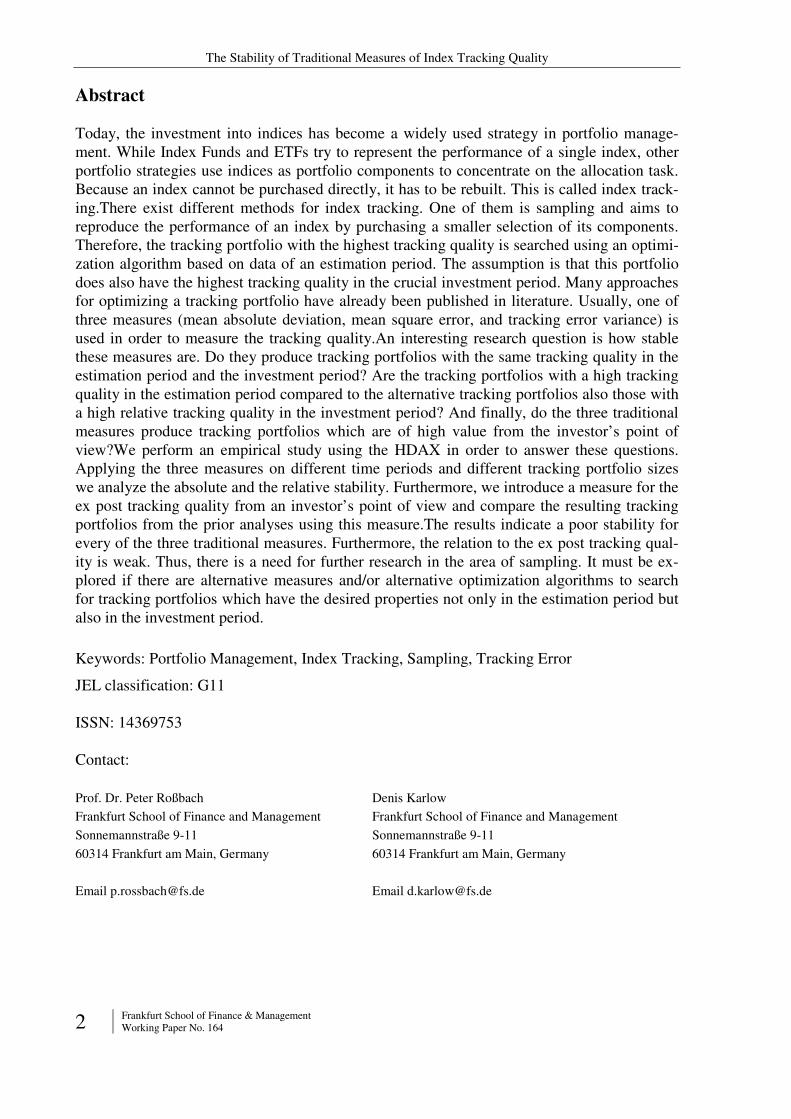
Abstract
Today, the investment into indices has become a widely used strategy in portfolio manage-ment. While Index Funds and ETFs try to represent the performance of a single index, other portfolio strategies use indices as portfolio components to concentrate on the allocation task. Because an index cannot be purchased directly, it has to be rebuilt. This is called index track-ing.There exist different methods for index tracking. One of them is sampling and aims to reproduce the performance of an index by purchasing a smaller selection of its components. Therefore, the tracking portfolio with the highest tracking quality is searched using an optimi-zation algorithm based on data of an estimation period. The assumption is that this portfolio does also have the highest tracking quality in the crucial investment period. Many approaches for optimizing a tracking portfolio have already been published in literature. Usually, one of three measures (mean absolute deviation, mean square error, and tracking error variance) is used in order to measure the tracking quality.An interesting research question is how stable these measures are. Do they produce tracking portfolios with the same tracking quality in the estimation period and the investment period? Are the tracking portfolios with a high tracking quality in the estimation period compared to the alternative tracking portfolios also those with a high relative tracking quality in the investment period? And finally, do the three traditional measures produce tracking portfolios which are of high value from the investor’s point of view?We perform an empirical study using the HDAX in order to answer these questions. Applying the three measures on different time periods and different tracking portfolio sizes we analyze the absolute and the relative stability. Furthermore, we introduce a measure for the ex post tracking quality from an investor’s point of view and compare the resulting tracking portfolios from the prior analyses using this measure.The results indicate a poor stability for every of the three traditional measures. Furthermore, the relation to the ex post tracking qual-ity is weak. Thus, there is a need for further research in the area of sampling. It must be ex-plored if there are alternative measures and/or alternative optimization algorithms to search for tracking portfolios which have the desired properties not only in the estimation period but also in the investment period.
Keywords: Portfolio Management, Index Tracking, Sampling, Tracking Error
JEL classification: G11
ISSN: 14369753
Contact:
Prof. Dr. Peter Roßbach
Frankfurt School of Finance and Management
Sonnemannstraße 9-11
60314 Frankfurt am Main, Germany
Email [email protected]
Denis Karlow
Frankfurt School of Finance and Management
Sonnemannstraße 9-11
60314 Frankfurt am Main, Germany
Email [email protected]

The Stability of Traditional Measures of Index Tracking Quality
Frankfurt School of Finance & Management Working Paper No. 164 3
Content
1 Introduction............................................................................................................................4
2 Methods of Index Tracking....................................................................................................4
3 Variants of Sampling .............................................................................................................5
4 Traditional Measures of Tracking Quality.............................................................................7
5 Analysis of the Stability of the Traditional Measures of Tracking Quality..........................9
5.1 Research Method ........................................................................................................9 5.2 Evaluation Method ...................................................................................................14 5.3 Empirical Results......................................................................................................15
6 Summary and Outlook .........................................................................................................34
References ................................................................................................................................36

The Stability of Traditional Meas-ures of Index Tracking Quality
4 Frankfurt School of Finance & Management Working Paper No. 164
1 Introduction
In the recent years, the investment into indices has become more and more popular. There is a huge growth in the number and volumes of passively managed index funds and exchange-traded funds (ETFs) that match the market performance.1 This is the consequence due to the empirical findings that it is very difficult for an actively managed portfolio to beat an index in the long term after cost of administration and analytics.2 But also in active portfolio manage-ment there exist empirical results that show that the allocation over countries or industrial sectors provides a greater contribution to the portfolio performance than the selection of sin-gle assets.3 The allocation task is usually done by using risk and return ratios of the indices representing the countries respectively sectors. As a consequence, one has to invest into these indices to achieve the desired risk-return-profile of the portfolio. In both cases, the investment into indices is a main task of the portfolio manager. But indices cannot be purchased directly. Instead, the portfolio manager has to rebuild the index he wants to invest into. This is called index tracking.
The term index tracking covers different methods which aim to reproduce an index of stocks, bonds, commodities, etc. Every method has its specific advantages and disadvantages. One of these methods, where the index is reproduced with a smaller number of assets, is called sam-pling. This so-called tracking portfolio is calculated using past data. The calculation is based on measures reflecting the tracking quality. It is assumed that a good tracking quality in the estimation period will also result in a good tracking quality in the following investment pe-riod.
The aim of this paper is to show that the traditional measures which are used to calculate the tracking portfolio have some weaknesses that are mainly subject to an overfitting effect. Hence, a good tracking quality in the estimation period does not guarantee a good tracking quality in the investment period.
In the next chapter, the methods of index tracking are discussed. Chapter 3 gives an overview over the variants of sampling. Chapter 4 introduces the traditional measures of tracking qual-ity used in sampling. In chapter 5 the results of an empirical analysis about the tracking qual-ity produced by these measures are presented. Finally, further research questions are dis-cussed.
2 Methods of Index Tracking
There exist three main methods of index tracking: full replication, synthetic replication and sampling.
When applying full replication, the index is exactly replicated; this means that all the underly-ing assets of the specific index with the corresponding weights have to be purchased.4 The advantage of this method is that the tracking portfolio is identical to the index. A disadvantage
1 See Fuhr/Kelly (2010), p. 11. 2 For example see Scharpe (1991), p. 7 and French (2008), p. 1538. 3 See Hopkins/Miller (2001), pp. 63-64. 4 See Rudd (1980), p. 58.
The Stability of Traditional Measures of Index Tracking Quality
Frankfurt School of Finance & Management Working Paper No. 164 5
is that this method can be very capital intensive. Depending on the number of underlying as-sets, like the S&P 500 or the Wilshire 5000, a huge amount of capital may be needed to com-pletely rebuild the index. If the amount is too small, e.g. if the tracking portfolio is just a part of an actively managed portfolio, the complete rebuild of the index is an impractical task. In many indices assets are replaced by others from time to time. In these cases the tracking port-folio must be revised in order to keep the full replication state, resulting in transaction costs.5 The amount of the necessary transaction costs depends on the frequency of revisions and can be relatively high. Moreover, the replacements are predictable and pre-announced. This leads to abnormal high prices for new assets and low prices for removed assets.6 In these cases, the goal of index tracking can not be accomplished.
Another popular method of index tracking is synthetic replication, which needs a counter-party. The issuer of the index fund or ETF constructs an in principle arbitrary portfolio and the counterparty agrees to pay the index return in exchange for a small fee and the returns on collateral held in the issuers portfolio.7 Usually, this is done using a swap, covering the differ-ence between the two returns. The advantage of this method is that one can achieve a perfect tracking at very low costs. Just the fee has to be paid. A disadvantage is the inherent counter-party risk, because only the counterparty's creditworthiness guarantees the return on the index. In the EU this risk is limited by regulations to a maximum of 10 percent exposure to the swap counterparty. That means that the fund manager has to have at least 90 percent collateral to back the swap. Otherwise, the collateral has to be revised, resulting in transaction costs. But in the event of the fund issuer’s insolvency only the collateral acts as a liability.
The third method of index tracking is sampling.8 Here, the index is reproduced by a tracking portfolio containing a smaller number of assets, mostly a subset of its components. As a con-sequence, the reproduction is imperfect. This imperfection can be measured by the so-called tracking error. This is the main disadvantage of the sampling method. The advantage is that a tracking portfolio can be built with only a small amount of capital with respect to an accept-able tracking error.
3 Variants of Sampling
When applying sampling, three questions have to be solved: (1) How many assets shall the tracking portfolio contain, (2) Which assets have to be chosen and (3) What weights should the chosen assets have? These questions result in a combinatorial problem with a huge num-ber of combinations depending on the index.
In practice, usually simple heuristics are applied. The simplest one is stratified sampling.9 Stratified sampling starts by dividing the index assets using one or a combination of charac-teristics. These could be the market capitalization and/or the industrial sectors, for example. In a very easy variant, the assets of the index are first ordered by their market capitalization. Then, the number of assets is chosen whereby a desired level of tracking quality is achieved. The weight of an asset in the tracking portfolio is calculated via the capitalization of the asset
5 See Schioldager et al. (2004), pp. 391-393. 6 See Chen et al. (2006), p. 31 and Blume/Edelen (2004), p. 37 7 See Hill/Mueller (2004), pp. 522-523. 8 See Montfort et al. (2008), p.144. 9 See Meade/Salkin (1989), p. 872.
The Stability of Traditional Measures of Index Tracking Quality
6 Frankfurt School of Finance & Management Working Paper No. 164
divided by the sum of the capitalizations of all selected assets. A more sophisticated variant of the stratified sampling first divides the index by its sectors. Then, the sectors are ordered by their market capitalization. In the tracking portfolio each sector is represented by the asset with the highest market capitalization. If there are more sectors than the desired number of assets in the tracking portfolio, the sectors with the lowest market capitalization are elimi-nated.
Another commonly used variant is optimized sampling.10 Again, at first a preset number of assets is chosen, e.g. by their market capitalization. Subsequently, the weights of these assets are calculated using an optimization algorithm, minimizing the divergence of the tracking portfolios return to the index return. Depending on the measure of divergence (linear or quad-ratic), different optimization algorithms are used.
Both sampling methods rely on the assumption that the assets chosen by the above mentioned heuristics have the strongest influence on the index. If this is not the case, there must be other asset combinations which may have a better tracking quality.
Depending on the size of the index, the number of all possible combinations can be enor-mously huge. For example, tracking the DAX 30 index with 15 out of its 30 stocks for exam-ple results in 155,117,520 possible combinations. One of these possible combinations has the best tracking quality. To find this one, every possible combination can be optimized and fi-nally the combination with the best tracking quality has to be chosen as the tracking portfolio. This procedure would require a huge amount of computing power and/or a huge amount of time. For bigger indices, the numbers of possible combinations are much larger.
To solve this combinatorial problem, usually meta-heuristics, like genetic algorithms11, threshold accepting12 or differential evolution13, are applied.14 These search methods are very efficient, even when large search spaces exist. They do not guarantee that the overall best combination will be found, but, with a proper setup, they are able to find solutions which are close to the overall optimum.
Several empirical studies show that the application of these methods results in tracking port-folios with a high tracking quality in the estimation period. Roßbach and Karlow have shown that a genetic algorithm clearly outperforms stratified sampling and optimized sampling.15 They applied the three methods to the DAX 30 and an artificial index based on the underlying assets of the DAX 30 with no changes in weights. The analysis was repeated for different time intervals from 1998 to 2008. In the estimation period the genetic algorithm always outper-
10 See Bonafede (2003), p. 5. 11 See Ruiz-Torrubiano/Suarez (2009), p. 58. 12 See Gilli/Kellezi (2001), p. 9. 13 See Maringer (2008), pp. 12-14. 14 In Literature, some additional approaches can be found. Alexander and Dimitriu (2004) select only stocks,
which have a strong cointegration with the index. Canakgoz and Beasley (2009) and Stoyan and Kwon (2010) use a mixed integer programming approach where the selection of the assets and the calculation of their weights for the optimal tracking portfolio is done simultaneously. Focardi and Fabozzi (2004) and Dose and Cincotti (2005) use time series clustering to build groups of similar stocks for further selection. Corielli and Marcellino (2006) apply a factor analysis to the index stocks and select those stocks which are mostly corre-lated to the resulting factors. Gaivoronski et al. (2005) first build a tracking portfolio with all assets in the in-dex and then select only the assets with the largest proportions.
15 See Roßbach/Karlow (2009).

The Stability of Traditional Measures of Index Tracking Quality
Frankfurt School of Finance & Management Working Paper No. 164 7
formed stratified sampling and optimized sampling. In the investment period a different result was achieved. Using the artificial index, the genetic algorithm was again able to sustainably find tracking portfolios of higher quality than the two other methods. However, using the real DAX 30, the genetic algorithm was worse in nearly half of the cases. Additionally, in all cases the tracking quality in the estimation period was clearly better than in the investment period. This indicates that the frequent changes of the weights of the DAX 30 performance index led to an overfitting effect when using the genetic algorithm. Thus, a high tracking quality in the estimation period does not guarantee a high tracking quality in the investment period.
This raises the question if the traditional measures of tracking quality are sufficient as an es-timator for the future tracking quality. To answer this question is the purpose of this study.
4 Traditional Measures of Tracking Quality
The majority of measures of tracking quality are based on the tracking error. The tracking error (TE) measures the difference between the returns of the tracking portfolio and the re-turns of the index. It can be formulated as
∑=
⋅−=−=n
1j
t,jjt,It,Pt,It rwrrrTE (1)
with pr = return of the tracking portfolio
Ir = return of the index
jr = return of asset j in the tracking portfolio
jw = weight of asset j in the tracking portfolio
n = number of assets in the tracking portfolio
and ∑=
=n
1j
j 1w
The measures of tracking quality are using the tracking error in different ways. One com-monly used measure is the mean absolute deviation (MAD), which measures the mean of the absolute differences between the returns over a given time interval
∑=
−⋅=T
1t
t,Pt,I rrT
1MAD (2)
with Tt ,,1 K= time periods.
The mean square error (MSE) expresses the tracking quality by measuring the mean of the squared differences between the returns over a given time interval
( )2T
1t
t,Pt,I rrT
1MSE ∑
=
−⋅= (3)
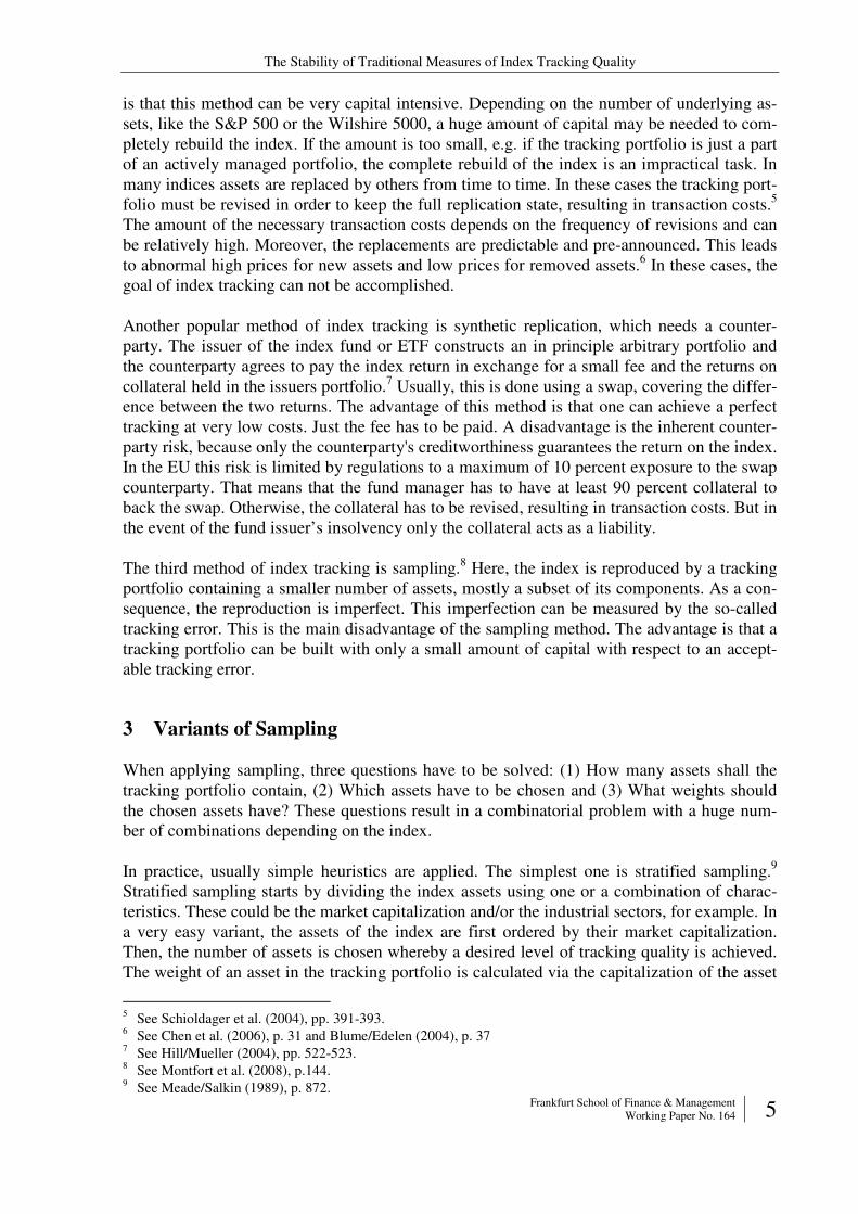
Figure 1 illustrates the difference between the MAD and the MSE. It can be seen that the MSE considers greater return differences relatively more than smaller ones compared to the MAD.
The Stability of Traditional Measures of Index Tracking Quality
8 Frankfurt School of Finance & Management Working Paper No. 164
0
1
2
3
4
5
6
7
8
9
-3 -2 -1 0 1 2 3
TE
MAD
MSE
0
1
2
3
4
5
6
7
8
9
-3 -2 -1 0 1 2 3
TE
MAD
MSE
Figure 1: Difference between MAD and MSE
A variant of the MSE is the tracking error variance (TEV), which is defined as the variance of the return differences
( )( )2T
1t
,PIt,Pt,I rrrrT
1TEV ∑
=
−−−⋅= (4)
with Pr = mean of returns of the tracking portfolio
Ir = mean of returns of the index
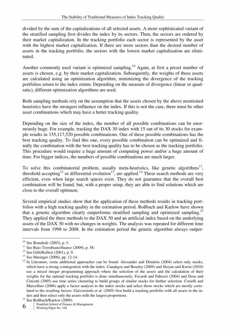
Even though the TEV is very often used, it has the disadvantage of a shift.16 That means, if the return of the tracking portfolio is always the same multiple to the return of the index, then the tracking error is a constant and the tracking error variance is zero, although there is a de-viation to the index. This is illustrated in Figure 2. Portfolio 1 has an obviously worse tracking quality than portfolio 2 but the TEV of Portfolio 1 is equal to zero while the TEV of Portfolio 2 is greater than zero.
-8,000%
-6,000%
-4,000%
-2,000%
0,000%
2,000%
4,000%
6,000%
8,000%
10,000%
Index Portfolio 1 Portfolio 2
TEV (Portfolio 1) = 0,000000%
TEV (Portfolio 2) = 0,002669%
-8,000%
-6,000%
-4,000%
-2,000%
0,000%
2,000%
4,000%
6,000%
8,000%
10,000%
Index Portfolio 1 Portfolio 2Index Portfolio 1 Portfolio 2
TEV (Portfolio 1) = 0,000000%
TEV (Portfolio 2) = 0,002669%
Retu
rn
Time Period
Figure 2: Weakness of the TEV
For a given selection of assets, the optimal tracking portfolio can be built by estimating the weights wj that minimize the chosen measure. But which one is the appropriate measure? 16 See Beasley et al. (2003), p. 629.
The Stability of Traditional Measures of Index Tracking Quality
Frankfurt School of Finance & Management Working Paper No. 164 9
From a mathematical point of view, the tracking error TE is an error term, usually denoted by εt. Thus, we can rewrite (1) as
∑=
+⋅=+=+=n
1j
tt,jjtt,Ptt,Pt,I rwrTErr εε (5)
The probabilistic characteristics of the error term have an essential influence on the estimation of the parameters wj. Thus, it can be shown that, if the error terms are IID17 and follow a nor-mal distribution, the minimization of the MSE gives the best linear unbiased estimator.18 But if the error terms are IID and follow a Laplace distribution, then it can be shown that the minimization of the MAD gives the most likely estimator. Rudolf et al. show that the different measures result in tracking portfolios with different risk/return properties.19 Rudolf concludes that MAD produces tracking portfolios, which are closer to the index in the investment pe-riod.20
In the remainder of the paper the robustness of the MAD, MSE and TEV will be analyzed. The focus lays on the analysis on how stable the estimations of tracking quality that are based on the minimization of these measures are.
5 Analysis of the Stability of the Traditional Measures of Tracking Quality
5.1 Research Method
In contrast to other studies on tracking quality, the focus of our research lies on the analysis of the stability of the measures described in the previous chapter. That means we are not search-ing for a method to find the best tracking portfolio with the highest tracking quality. Instead, we want to compare the results for the estimation periods with those for the investment peri-ods to prove the stability of the measures. Thus, the quality of the selection process in sam-pling does not play a role in this context.
We are interested in three topics. The first one is the comparison of the absolute tracking qual-ity in the estimation period and the investment period. That means we want to examine the difference in the level of tracking quality. The second topic is the comparison of the relative positions of the tracking portfolios in both time periods ranked by their quality. If a tracking portfolio affiliates to the best ones in the estimation period, does it also do that in the invest-ment period and vice versa? The third topic is a comparison of the ex post tracking qualities of the three traditional measures to evaluate if there are any significant differences in their predictive value.
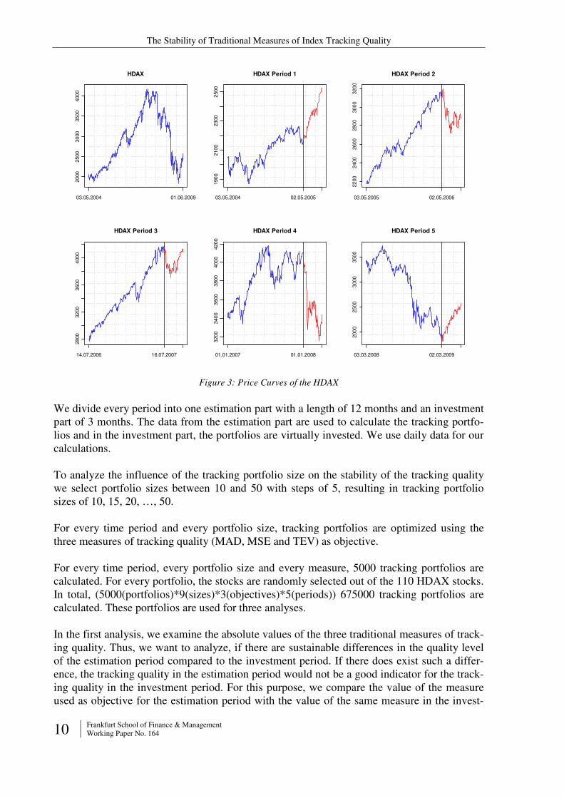
For our analysis, we use the HDAX performance index having 110 underlying German stocks. To avoid conclusions caused by specific capital market situations, we select different time periods between 2004 and 2010. Every time period covers a different capital market situation (see figure 3).
17 Independent and Identically Distributed. 18 See Draper/Smith (1998), p. 567. 19 See Rudolf/Wolter/Zimmermann (1999), p. 102. 20 See Rudolf (2009).
The Stability of Traditional Measures of Index Tracking Quality
10 Frankfurt School of Finance & Management Working Paper No. 164
03.05.2004 01.06.2009
2000
2500
3000
3500
4000
HDAX
03.05.2004 02.05.2005
1900
2100
2300
2500
HDAX Period 1
03.05.2005 02.05.2006
2200
2400
2600
2800
3000
3200
HDAX Period 2
14.07.2006 16.07.2007
2800
3200
3600
4000
HDAX Period 3
01.01.2007 01.01.2008
3200
3400
3600
3800
4000
4200
HDAX Period 4
03.03.2008 02.03.20092000
2500
3000
3500
HDAX Period 5
Figure 3: Price Curves of the HDAX
We divide every period into one estimation part with a length of 12 months and an investment part of 3 months. The data from the estimation part are used to calculate the tracking portfo-lios and in the investment part, the portfolios are virtually invested. We use daily data for our calculations.
To analyze the influence of the tracking portfolio size on the stability of the tracking quality we select portfolio sizes between 10 and 50 with steps of 5, resulting in tracking portfolio sizes of 10, 15, 20, …, 50.
For every time period and every portfolio size, tracking portfolios are optimized using the three measures of tracking quality (MAD, MSE and TEV) as objective.
For every time period, every portfolio size and every measure, 5000 tracking portfolios are calculated. For every portfolio, the stocks are randomly selected out of the 110 HDAX stocks. In total, (5000(portfolios)*9(sizes)*3(objectives)*5(periods)) 675000 tracking portfolios are calculated. These portfolios are used for three analyses.
In the first analysis, we examine the absolute values of the three traditional measures of track-ing quality. Thus, we want to analyze, if there are sustainable differences in the quality level of the estimation period compared to the investment period. If there does exist such a differ-ence, the tracking quality in the estimation period would not be a good indicator for the track-ing quality in the investment period. For this purpose, we compare the value of the measure used as objective for the estimation period with the value of the same measure in the invest-
The Stability of Traditional Measures of Index Tracking Quality
Frankfurt School of Finance & Management Working Paper No. 164 11
ment period. We calculate means and variances for every combination of portfolio size, time period and objective.
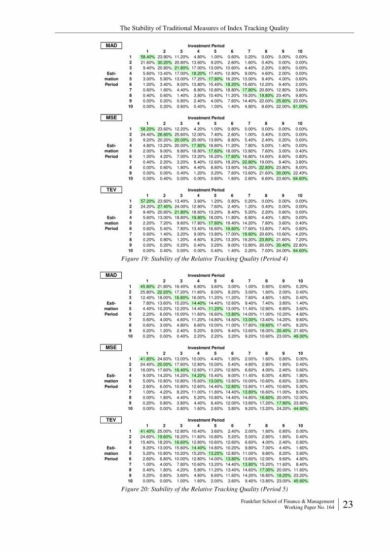
In the second analysis, we evaluate the stability of the relative tracking quality of the meas-ures used as objective. Therefore, we use each of the 5000 tracking portfolios for every com-bination of portfolio size, time period and objective, rank them according to their tracking quality in the estimation and in the investment period and finally allocate the portfolios into deciles for both time periods according to the ranks. The resulting tables indicate a bad stabil-ity if a high percentage of the tracking portfolios do not remain in the same deciles in the es-timation and the investment period.
The third analysis is a comparison of the ex post tracking qualities of the measures used as objectives. One important question is how to measure the quality in this context. First, it must be a measure to evaluate the ex post tracking quality in the view of an investor. Second, it does not seem to be advisable using a measure, which is used in parts of the optimizations when creating the tracking portfolios. We assume that such an ex post measure prefers the tracking portfolios built with the same measure used as objective.
For an investor, a tracking portfolio is of high quality if it performs similarly to the index. Similarity means in this context, that the tracking portfolio and the index do not really deviate from each other in the growth of value. The more similar a tracking portfolio is the higher quality it has for the investor.
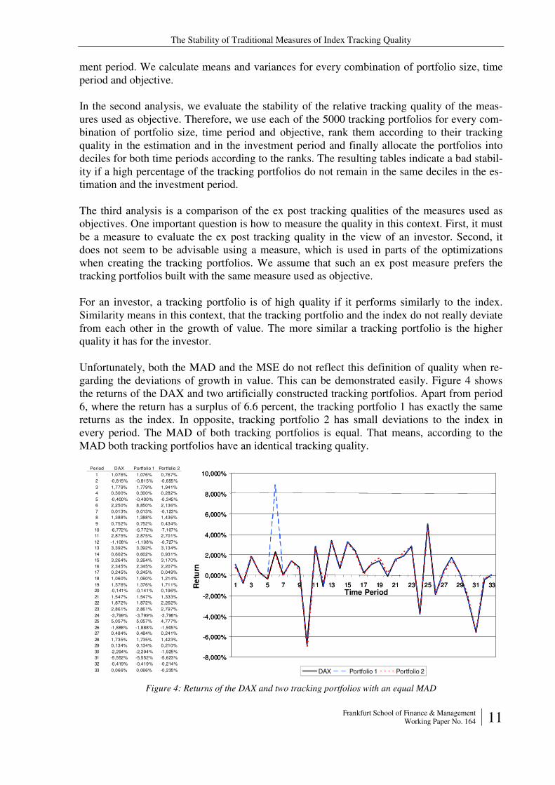
Unfortunately, both the MAD and the MSE do not reflect this definition of quality when re-garding the deviations of growth in value. This can be demonstrated easily. Figure 4 shows the returns of the DAX and two artificially constructed tracking portfolios. Apart from period 6, where the return has a surplus of 6.6 percent, the tracking portfolio 1 has exactly the same returns as the index. In opposite, tracking portfolio 2 has small deviations to the index in every period. The MAD of both tracking portfolios is equal. That means, according to the MAD both tracking portfolios have an identical tracking quality.
Period DAX Portfolio 1 Portfol io 2
1 1,076% 1,076% 0,767%
2 -0,815% -0,815% -0,655%
3 1,779% 1,779% 1,941%
4 0,300% 0,300% 0,282%
5 -0,400% -0,400% -0,345%
6 2,250% 8,850% 2,136%
7 0,013% 0,013% -0,123%
8 1,388% 1,388% 1,436%
9 0,752% 0,752% 0,434%
10 -6,772% -6,772% -7,107%
11 2,875% 2,875% 2,701%
12 -1,108% -1,108% -0,727%
13 3,392% 3,392% 3,134%
14 0,602% 0,602% 0,931%
15 3,264% 3,264% 3,170%
16 2,345% 2,345% 2,207%
17 0,245% 0,245% 0,049%
18 1,060% 1,060% 1,214%
19 1,376% 1,376% 1,711%
20 -0,141% -0,141% 0,196%
21 1,547% 1,547% 1,333%
22 1,872% 1,872% 2,262%
23 2,861% 2,861% 2,797%
24 -3,799% -3,799% -3,798%
25 5,057% 5,057% 4,777%
26 -1,888% -1,888% -1,905%
27 0,484% 0,484% 0,241%
28 1,735% 1,735% 1,423%
29 0,134% 0,134% 0,210%
30 -2,294% -2,294% -1,925%
31 -5,552% -5,552% -5,623%
32 -0,419% -0,419% -0,214%
33 0,066% 0,066% -0,235%
-8,000%
-6,000%
-4,000%
-2,000%
0,000%
2,000%
4,000%
6,000%
8,000%
10,000%
1 3 5 7 9 11 13 15 17 19 21 23 25 27 29 31 33
DAX Portfolio 1 Portfolio 2
-8,000%
-6,000%
-4,000%
-2,000%
0,000%
2,000%
4,000%
6,000%
8,000%
10,000%
1 3 5 7 9 11 13 15 17 19 21 23 25 27 29 31 33
DAX Portfolio 1 Portfolio 2
Re
turn
Time Period
Figure 4: Returns of the DAX and two tracking portfolios with an equal MAD
The Stability of Traditional Measures of Index Tracking Quality
12 Frankfurt School of Finance & Management Working Paper No. 164
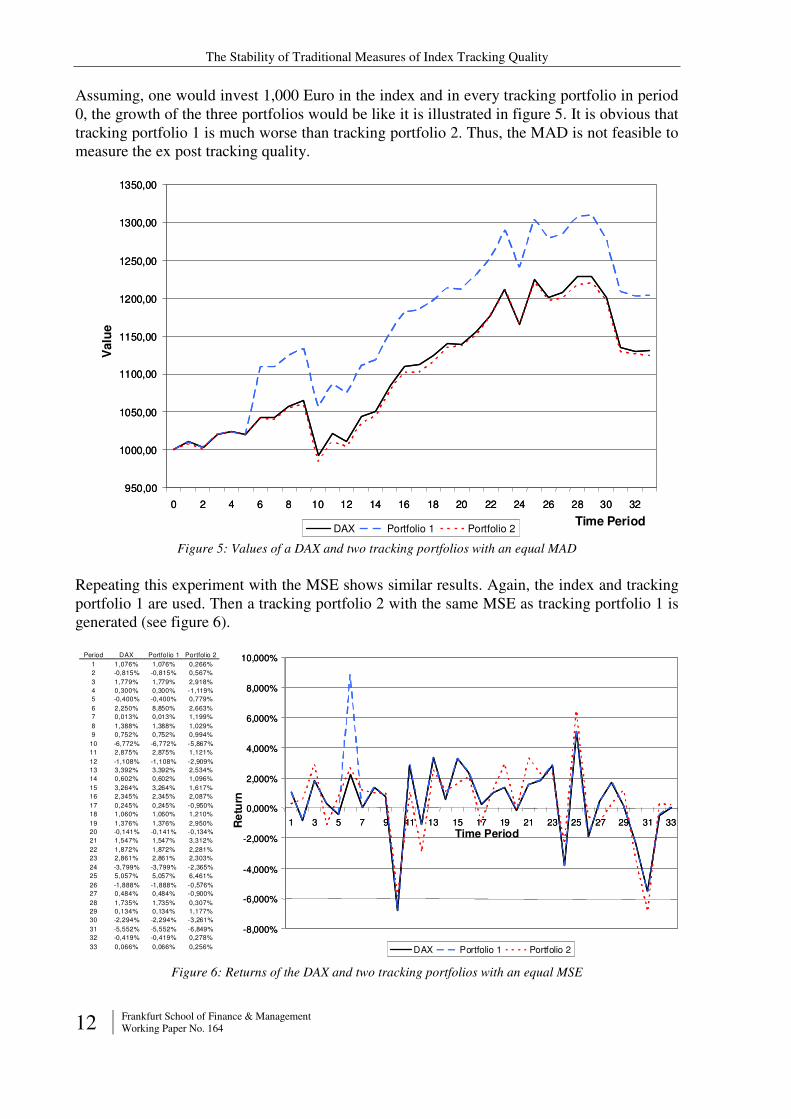
Assuming, one would invest 1,000 Euro in the index and in every tracking portfolio in period 0, the growth of the three portfolios would be like it is illustrated in figure 5. It is obvious that tracking portfolio 1 is much worse than tracking portfolio 2. Thus, the MAD is not feasible to measure the ex post tracking quality.
950,00
1000,00
1050,00
1100,00
1150,00
1200,00
1250,00
1300,00
1350,00
0 2 4 6 8 10 12 14 16 18 20 22 24 26 28 30 32
DAX Portfolio 1 Portfolio 2
950,00
1000,00
1050,00
1100,00
1150,00
1200,00
1250,00
1300,00
1350,00
0 2 4 6 8 10 12 14 16 18 20 22 24 26 28 30 32
DAX Portfolio 1 Portfolio 2
Valu
e
Time Period
Figure 5: Values of a DAX and two tracking portfolios with an equal MAD
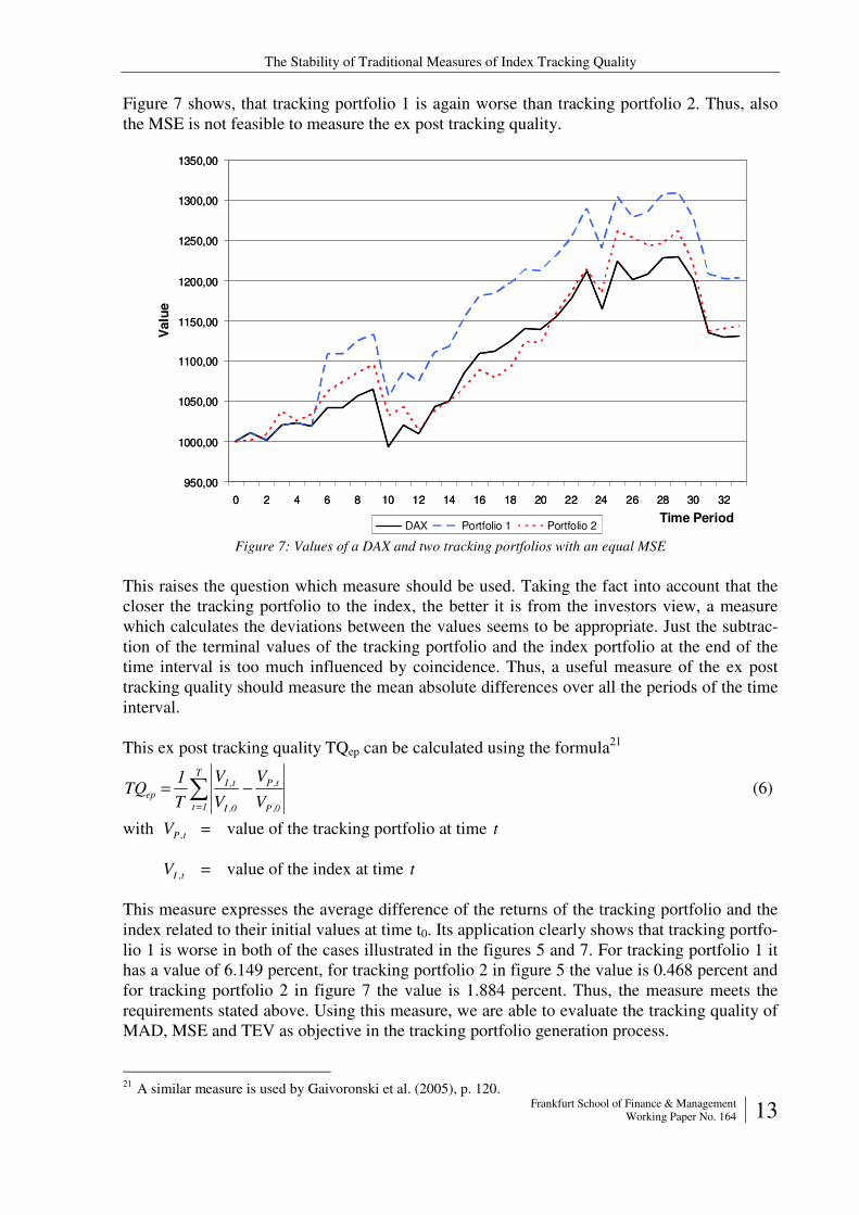
Repeating this experiment with the MSE shows similar results. Again, the index and tracking portfolio 1 are used. Then a tracking portfolio 2 with the same MSE as tracking portfolio 1 is generated (see figure 6).
-8,000%
-6,000%
-4,000%
-2,000%
0,000%
2,000%
4,000%
6,000%
8,000%
10,000%
1 3 5 7 9 11 13 15 17 19 21 23 25 27 29 31 33
DAX Portfolio 1 Portfolio 2
-8,000%
-6,000%
-4,000%
-2,000%
0,000%
2,000%
4,000%
6,000%
8,000%
10,000%
1 3 5 7 9 11 13 15 17 19 21 23 25 27 29 31 33
DAX Portfolio 1 Portfolio 2
Period DAX Portfol io 1 Portfol io 2
1 1,076% 1,076% 0,266%
2 -0,815% -0,815% 0,567%
3 1,779% 1,779% 2,918%
4 0,300% 0,300% -1,119%
5 -0,400% -0,400% 0,779%
6 2,250% 8,850% 2,663%
7 0,013% 0,013% 1,199%
8 1,388% 1,388% 1,029%
9 0,752% 0,752% 0,994%
10 -6,772% -6,772% -5,867%
11 2,875% 2,875% 1,121%
12 -1,108% -1,108% -2,909%
13 3,392% 3,392% 2,534%
14 0,602% 0,602% 1,096%
15 3,264% 3,264% 1,617%
16 2,345% 2,345% 2,087%
17 0,245% 0,245% -0,950%
18 1,060% 1,060% 1,210%
19 1,376% 1,376% 2,950%
20 -0,141% -0,141% -0,134%
21 1,547% 1,547% 3,312%
22 1,872% 1,872% 2,281%
23 2,861% 2,861% 2,303%
24 -3,799% -3,799% -2,365%
25 5,057% 5,057% 6,461%
26 -1,888% -1,888% -0,576%
27 0,484% 0,484% -0,900%
28 1,735% 1,735% 0,307%
29 0,134% 0,134% 1,177%
30 -2,294% -2,294% -3,261%
31 -5,552% -5,552% -6,849%
32 -0,419% -0,419% 0,278%
33 0,066% 0,066% 0,256%
Re
turn
Time Period
Figure 6: Returns of the DAX and two tracking portfolios with an equal MSE
The Stability of Traditional Measures of Index Tracking Quality
Frankfurt School of Finance & Management Working Paper No. 164 13
Figure 7 shows, that tracking portfolio 1 is again worse than tracking portfolio 2. Thus, also the MSE is not feasible to measure the ex post tracking quality.
950,00
1000,00
1050,00
1100,00
1150,00
1200,00
1250,00
1300,00
1350,00
0 2 4 6 8 10 12 14 16 18 20 22 24 26 28 30 32
DAX Portfolio 1 Portfolio 2
950,00
1000,00
1050,00
1100,00
1150,00
1200,00
1250,00
1300,00
1350,00
0 2 4 6 8 10 12 14 16 18 20 22 24 26 28 30 32
DAX Portfolio 1 Portfolio 2
Valu
e
Time Period
Figure 7: Values of a DAX and two tracking portfolios with an equal MSE
This raises the question which measure should be used. Taking the fact into account that the closer the tracking portfolio to the index, the better it is from the investors view, a measure which calculates the deviations between the values seems to be appropriate. Just the subtrac-tion of the terminal values of the tracking portfolio and the index portfolio at the end of the time interval is too much influenced by coincidence. Thus, a useful measure of the ex post tracking quality should measure the mean absolute differences over all the periods of the time interval.
This ex post tracking quality TQep can be calculated using the formula21
∑=
−=T
1t 0,P
t,P
0,I
t,I
epV
V
V
V
T
1TQ (6)
with tPV , = value of the tracking portfolio at time t
tIV , = value of the index at time t
This measure expresses the average difference of the returns of the tracking portfolio and the index related to their initial values at time t0. Its application clearly shows that tracking portfo-lio 1 is worse in both of the cases illustrated in the figures 5 and 7. For tracking portfolio 1 it has a value of 6.149 percent, for tracking portfolio 2 in figure 5 the value is 0.468 percent and for tracking portfolio 2 in figure 7 the value is 1.884 percent. Thus, the measure meets the requirements stated above. Using this measure, we are able to evaluate the tracking quality of MAD, MSE and TEV as objective in the tracking portfolio generation process.
21 A similar measure is used by Gaivoronski et al. (2005), p. 120.
The Stability of Traditional Measures of Index Tracking Quality
14 Frankfurt School of Finance & Management Working Paper No. 164
5.2 Evaluation Method
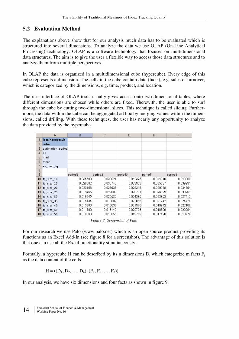
The explanations above show that for our analysis much data has to be evaluated which is structured into several dimensions. To analyze the data we use OLAP (On-Line Analytical Processing) technology. OLAP is a software technology that focuses on multidimensional data structures. The aim is to give the user a flexible way to access those data structures and to analyze them from multiple perspectives.
In OLAP the data is organized in a multidimensional cube (hypercube). Every edge of this cube represents a dimension. The cells in the cube contain data (facts), e.g. sales or turnover, which is categorized by the dimensions, e.g. time, product, and location.
The user interface of OLAP tools usually gives access onto two-dimensional tables, where different dimensions are chosen while others are fixed. Therewith, the user is able to surf through the cube by cutting two-dimensional slices. This technique is called slicing. Further-more, the data within the cube can be aggregated ad hoc by merging values within the dimen-sions, called drilling. With these techniques, the user has nearly any opportunity to analyze the data provided by the hypercube.
Figure 8: Screenshot of Palo
For our research we use Palo (www.palo.net) which is an open source product providing its functions as an Excel Add-In (see figure 8 for a screenshot). The advantage of this solution is that one can use all the Excel functionality simultaneously.
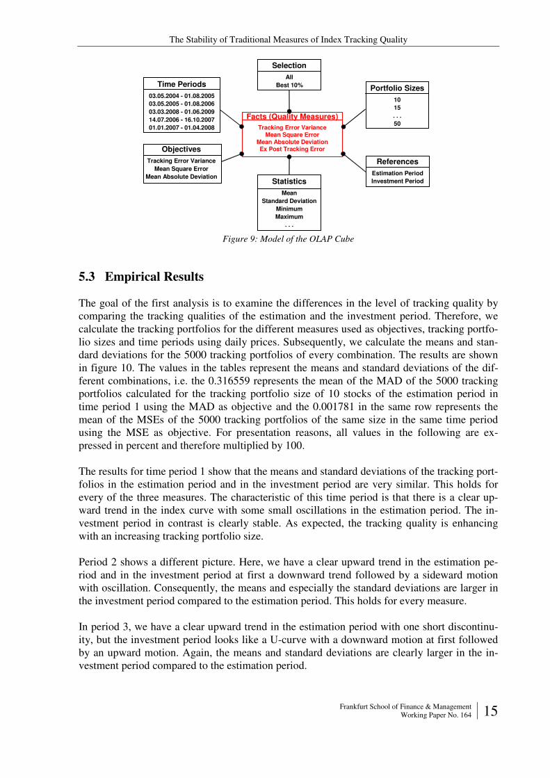
Formally, a hypercube H can be described by its n dimensions Di which categorize m facts Fj as the data content of the cells
H = ((D1, D2, …, Dn), (F1, F2, …, Fn))
In our analysis, we have six dimensions and four facts as shown in figure 9.
The Stability of Traditional Measures of Index Tracking Quality
Frankfurt School of Finance & Management Working Paper No. 164 15
Time Periods
03.05.2004 - 01.08.2005
03.05.2005 - 01.08.2006
03.03.2008 - 01.06.2009
14.07.2006 - 16.10.2007
01.01.2007 - 01.04.2008
Facts (Quality Measures)
Tracking Error VarianceMean Square Error
Mean Absolute DeviationEx Post Tracking ErrorObjectives
Tracking Error Variance
Mean Square Error
Mean Absolute Deviation
References
Estimation Period
Investment Period
Portfolio Sizes
10
15
. . .
50
Selection
All
Best 10%
Statistics
Mean
Standard Deviation
Minimum
Maximum
. . . Figure 9: Model of the OLAP Cube
5.3 Empirical Results
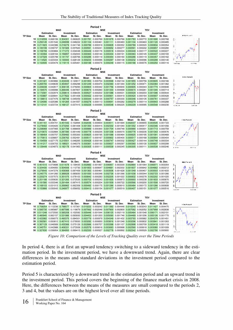
The goal of the first analysis is to examine the differences in the level of tracking quality by comparing the tracking qualities of the estimation and the investment period. Therefore, we calculate the tracking portfolios for the different measures used as objectives, tracking portfo-lio sizes and time periods using daily prices. Subsequently, we calculate the means and stan-dard deviations for the 5000 tracking portfolios of every combination. The results are shown in figure 10. The values in the tables represent the means and standard deviations of the dif-ferent combinations, i.e. the 0.316559 represents the mean of the MAD of the 5000 tracking portfolios calculated for the tracking portfolio size of 10 stocks of the estimation period in time period 1 using the MAD as objective and the 0.001781 in the same row represents the mean of the MSEs of the 5000 tracking portfolios of the same size in the same time period using the MSE as objective. For presentation reasons, all values in the following are ex-pressed in percent and therefore multiplied by 100.
The results for time period 1 show that the means and standard deviations of the tracking port-folios in the estimation period and in the investment period are very similar. This holds for every of the three measures. The characteristic of this time period is that there is a clear up-ward trend in the index curve with some small oscillations in the estimation period. The in-vestment period in contrast is clearly stable. As expected, the tracking quality is enhancing with an increasing tracking portfolio size.
Period 2 shows a different picture. Here, we have a clear upward trend in the estimation pe-riod and in the investment period at first a downward trend followed by a sideward motion with oscillation. Consequently, the means and especially the standard deviations are larger in the investment period compared to the estimation period. This holds for every measure.
In period 3, we have a clear upward trend in the estimation period with one short discontinu-ity, but the investment period looks like a U-curve with a downward motion at first followed by an upward motion. Again, the means and standard deviations are clearly larger in the in-vestment period compared to the estimation period.
The Stability of Traditional Measures of Index Tracking Quality
16 Frankfurt School of Finance & Management Working Paper No. 164
TP Size Mean St. Dev. Mean St. Dev. Mean St. Dev. Mean St. Dev. Mean St. Dev. Mean St. Dev.
10 0.316559 0.068156 0.304301 0.060625 0.001781 0.000769 0.001678 0.000766 0.001783 0.000772 0.001690 0.000768
15 0.250145 0.051542 0.249099 0.048222 0.001104 0.000461 0.001111 0.000483 0.001104 0.000463 0.001120 0.000485
20 0.211823 0.042386 0.216279 0.041746 0.000789 0.000319 0.000828 0.000352 0.000789 0.000320 0.000834 0.000354
25 0.183199 0.036737 0.191926 0.037620 0.000591 0.000241 0.000652 0.000277 0.000591 0.000242 0.000657 0.000280
30 0.159706 0.030884 0.171272 0.034048 0.000449 0.000176 0.000518 0.000224 0.000449 0.000177 0.000522 0.000227
35 0.143394 0.028164 0.156857 0.032003 0.000363 0.000144 0.000434 0.000191 0.000363 0.000145 0.000437 0.000193
40 0.127029 0.025799 0.141747 0.029766 0.000286 0.000119 0.000354 0.000160 0.000286 0.000119 0.000357 0.000162
45 0.114520 0.023334 0.130000 0.028129 0.000233 0.000096 0.000297 0.000138 0.000232 0.000096 0.000299 0.000140
50 0.102935 0.020476 0.119115 0.025461 0.000188 0.000076 0.000249 0.000115 0.000188 0.000076 0.000250 0.000116
TP Size Mean St. Dev. Mean St. Dev. Mean St. Dev. Mean St. Dev. Mean St. Dev. Mean St. Dev.
10 0.331421 0.063882 0.434049 0.120817 0.001953 0.000754 0.003568 0.002134 0.001955 0.000756 0.003605 0.002166
15 0.265700 0.049639 0.353937 0.094298 0.001249 0.000470 0.002360 0.001340 0.001252 0.000471 0.002384 0.001362
20 0.226038 0.042617 0.306135 0.079283 0.000904 0.000342 0.001756 0.000930 0.000905 0.000343 0.001774 0.000948
25 0.194570 0.036996 0.266446 0.067907 0.000673 0.000260 0.001333 0.000699 0.000674 0.000261 0.001345 0.000714
30 0.172091 0.032974 0.239614 0.058435 0.000527 0.000202 0.001088 0.000531 0.000529 0.000203 0.001096 0.000544
35 0.153887 0.029941 0.217822 0.051408 0.000422 0.000164 0.000901 0.000419 0.000424 0.000164 0.000907 0.000428
40 0.138613 0.027476 0.198748 0.045059 0.000344 0.000135 0.000757 0.000330 0.000346 0.000135 0.000761 0.000337
45 0.124090 0.025386 0.181265 0.041557 0.000278 0.000113 0.000641 0.000282 0.000279 0.000114 0.000643 0.000288
50 0.112141 0.023724 0.166127 0.037415 0.000228 0.000095 0.000548 0.000225 0.000229 0.000095 0.000548 0.000230
TP Size Mean St. Dev. Mean St. Dev. Mean St. Dev. Mean St. Dev. Mean St. Dev. Mean St. Dev.
10 0.341161 0.054701 0.451542 0.102894 0.002036 0.000654 0.003511 0.001694 0.002037 0.000655 0.003535 0.001723
15 0.278402 0.043420 0.373293 0.081408 0.001350 0.000415 0.002332 0.001040 0.001352 0.000417 0.002346 0.001056
20 0.238069 0.037065 0.321788 0.068809 0.000989 0.000300 0.001704 0.000748 0.000990 0.000301 0.001713 0.000759
25 0.210672 0.032884 0.287390 0.061449 0.000778 0.000235 0.001338 0.000570 0.000778 0.000235 0.001343 0.000576
30 0.188454 0.030707 0.259482 0.055300 0.000625 0.000195 0.001088 0.000464 0.000625 0.000195 0.001091 0.000469
35 0.170613 0.028807 0.236762 0.052481 0.000517 0.000167 0.000902 0.000400 0.000517 0.000168 0.000904 0.000404
40 0.154559 0.027175 0.215501 0.048265 0.000428 0.000144 0.000747 0.000332 0.000427 0.000144 0.000748 0.000334
45 0.141217 0.026703 0.198021 0.046376 0.000361 0.000130 0.000637 0.000297 0.000360 0.000130 0.000637 0.000299
50 0.129449 0.024873 0.182178 0.041963 0.000305 0.000111 0.000539 0.000245 0.000305 0.000111 0.000539 0.000246
TP Size Mean St. Dev. Mean St. Dev. Mean St. Dev. Mean St. Dev. Mean St. Dev. Mean St. Dev.
10 0.401510 0.070688 0.611678 0.139435 0.002882 0.001067 0.006957 0.003330 0.002864 0.001064 0.006971 0.003354
15 0.324430 0.054950 0.504006 0.112730 0.001853 0.000647 0.004661 0.002202 0.001837 0.000642 0.004662 0.002212
20 0.279543 0.047276 0.439368 0.097459 0.001363 0.000461 0.003506 0.001628 0.001349 0.000457 0.003503 0.001633
25 0.245775 0.041260 0.389028 0.085830 0.001050 0.000348 0.002726 0.001266 0.001038 0.000344 0.002723 0.001266
30 0.220274 0.037573 0.351075 0.078103 0.000842 0.000283 0.002205 0.001022 0.000832 0.000278 0.002202 0.001020
35 0.201188 0.035630 0.321265 0.072535 0.000703 0.000243 0.001835 0.000873 0.000693 0.000238 0.001833 0.000870
40 0.181580 0.033346 0.291494 0.067415 0.000574 0.000204 0.001509 0.000722 0.000566 0.000200 0.001508 0.000720
45 0.168103 0.031013 0.269962 0.062358 0.000492 0.000175 0.001286 0.000610 0.000484 0.000172 0.001286 0.000608
50 0.153866 0.030043 0.246977 0.059052 0.000413 0.000154 0.001077 0.000519 0.000407 0.000151 0.001077 0.000516
TP Size Mean St. Dev. Mean St. Dev. Mean St. Dev. Mean St. Dev. Mean St. Dev. Mean St. Dev.
10 0.708254 0.112236 0.798577 0.157361 0.010222 0.003242 0.011362 0.004446 0.010245 0.003243 0.011427 0.004475
15 0.585735 0.085887 0.667086 0.119879 0.007062 0.002048 0.007900 0.002800 0.007082 0.002052 0.007958 0.002838
20 0.511248 0.072550 0.585208 0.102592 0.005446 0.001544 0.006125 0.002119 0.005464 0.001548 0.006171 0.002151
25 0.460945 0.062157 0.531986 0.093930 0.004453 0.001203 0.005090 0.001746 0.004469 0.001206 0.005126 0.001770
30 0.422982 0.056073 0.490375 0.084501 0.003779 0.000979 0.004349 0.001432 0.003793 0.000982 0.004379 0.001451
35 0.392581 0.050812 0.457410 0.079550 0.003282 0.000830 0.003816 0.001248 0.003296 0.000832 0.003841 0.001263
40 0.367129 0.046569 0.430366 0.075126 0.002886 0.000707 0.003398 0.001107 0.002898 0.000709 0.003418 0.001119
45 0.345751 0.042988 0.406331 0.072938 0.002578 0.000616 0.003063 0.000998 0.002590 0.000618 0.003080 0.001009
50 0.327630 0.038954 0.384950 0.069415 0.002330 0.000527 0.002778 0.000892 0.002342 0.000529 0.002790 0.000900
Estimation InvestmentEstimation Investment Estimation Investment
Estimation Investment
Period 5MAD MSE TEV
Estimation Investment Estimation Investment
Estimation Investment
Period 4MAD MSE TEV
Estimation Investment Estimation Investment
Period 3MAD MSE TEV
Investment Estimation Investment
Period 2
Estimation Investment Estimation
MAD MSE TEV
Estimation InvestmentInvestment Estimation Investment Estimation
Period 1MAD MSE TEV
Figure 10: Comparison of the Levels of Tracking Quality over the Time Periods
In period 4, there is at first an upward tendency switching to a sideward tendency in the esti-mation period. In the investment period, we have a downward trend. Again, there are clear differences in the means and standard deviations in the investment period compared to the estimation period.
Period 5 is characterized by a downward trend in the estimation period and an upward trend in the investment period. This period covers the beginning of the finance market crisis in 2008. Here, the differences between the means of the measures are small compared to the periods 2, 3 and 4, but the values are on the highest level over all time periods.
The Stability of Traditional Measures of Index Tracking Quality
Frankfurt School of Finance & Management Working Paper No. 164 17
TP Size Period 1 Period 2 Period 3 Period 4 Period 5
10 0.316559 0.331421 0.341161 0.401510 0.708254
15 0.250145 0.265700 0.278402 0.324430 0.585735
20 0.211823 0.226038 0.238069 0.279543 0.511248
25 0.183199 0.194570 0.210672 0.245775 0.460945
30 0.159706 0.172091 0.188454 0.220274 0.422982
35 0.143394 0.153887 0.170613 0.201188 0.392581
40 0.127029 0.138613 0.154559 0.181580 0.367129
45 0.114520 0.124090 0.141217 0.168103 0.345751
50 0.102935 0.112141 0.129449 0.153866 0.327630
TP Size Period 1 Period 2 Period 3 Period 4 Period 5
10 0.001781 0.001953 0.002036 0.002882 0.010222
15 0.001104 0.001249 0.001350 0.001853 0.007062
20 0.000789 0.000904 0.000989 0.001363 0.005446
25 0.000591 0.000673 0.000778 0.001050 0.004453
30 0.000449 0.000527 0.000625 0.000842 0.003779
35 0.000363 0.000422 0.000517 0.000703 0.003282
40 0.000286 0.000344 0.000428 0.000574 0.002886
45 0.000233 0.000278 0.000361 0.000492 0.002578
50 0.000188 0.000228 0.000305 0.000413 0.002330
TP Size Period 1 Period 2 Period 3 Period 4 Period 5
10 0.001783 0.001955 0.002037 0.002864 0.010245
15 0.001104 0.001252 0.001352 0.001837 0.007082
20 0.000789 0.000905 0.000990 0.001349 0.005464
25 0.000591 0.000674 0.000778 0.001038 0.004469
30 0.000449 0.000529 0.000625 0.000832 0.003793
35 0.000363 0.000424 0.000517 0.000693 0.003296
40 0.000286 0.000346 0.000427 0.000566 0.002898
45 0.000232 0.000279 0.000360 0.000484 0.002590
50 0.000188 0.000229 0.000305 0.000407 0.002342
MAD
TEV
MSE
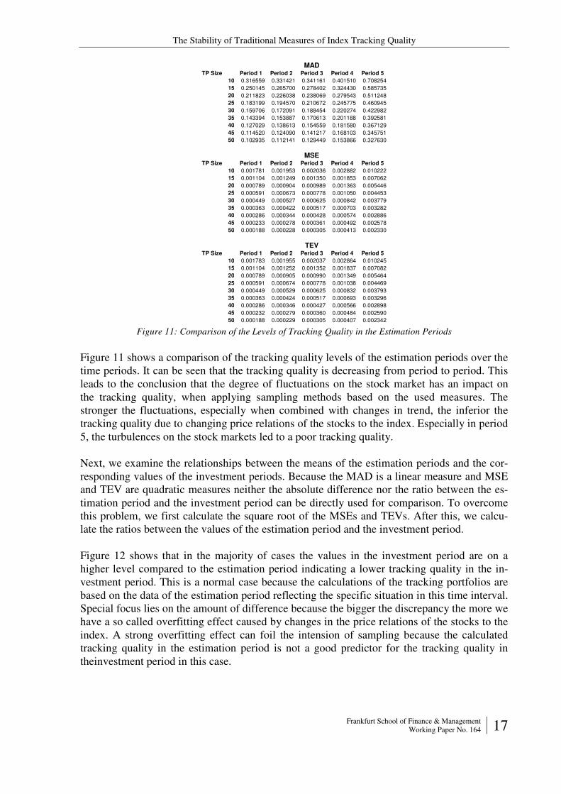
Figure 11: Comparison of the Levels of Tracking Quality in the Estimation Periods
Figure 11 shows a comparison of the tracking quality levels of the estimation periods over the time periods. It can be seen that the tracking quality is decreasing from period to period. This leads to the conclusion that the degree of fluctuations on the stock market has an impact on the tracking quality, when applying sampling methods based on the used measures. The stronger the fluctuations, especially when combined with changes in trend, the inferior the tracking quality due to changing price relations of the stocks to the index. Especially in period 5, the turbulences on the stock markets led to a poor tracking quality.
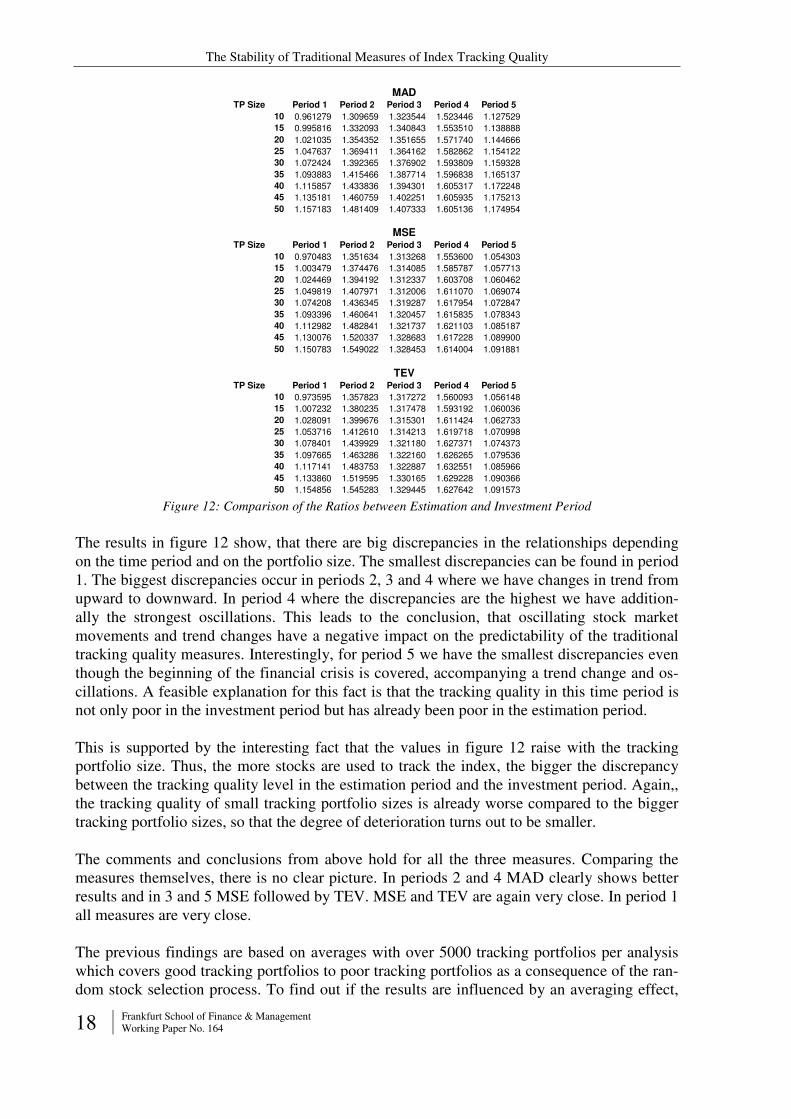
Next, we examine the relationships between the means of the estimation periods and the cor-responding values of the investment periods. Because the MAD is a linear measure and MSE and TEV are quadratic measures neither the absolute difference nor the ratio between the es-timation period and the investment period can be directly used for comparison. To overcome this problem, we first calculate the square root of the MSEs and TEVs. After this, we calcu-late the ratios between the values of the estimation period and the investment period.
Figure 12 shows that in the majority of cases the values in the investment period are on a higher level compared to the estimation period indicating a lower tracking quality in the in-vestment period. This is a normal case because the calculations of the tracking portfolios are based on the data of the estimation period reflecting the specific situation in this time interval. Special focus lies on the amount of difference because the bigger the discrepancy the more we have a so called overfitting effect caused by changes in the price relations of the stocks to the index. A strong overfitting effect can foil the intension of sampling because the calculated tracking quality in the estimation period is not a good predictor for the tracking quality in theinvestment period in this case.
The Stability of Traditional Measures of Index Tracking Quality
18 Frankfurt School of Finance & Management Working Paper No. 164
TP Size Period 1 Period 2 Period 3 Period 4 Period 5
10 0.961279 1.309659 1.323544 1.523446 1.127529
15 0.995816 1.332093 1.340843 1.553510 1.138888
20 1.021035 1.354352 1.351655 1.571740 1.144666
25 1.047637 1.369411 1.364162 1.582862 1.154122
30 1.072424 1.392365 1.376902 1.593809 1.159328
35 1.093883 1.415466 1.387714 1.596838 1.165137
40 1.115857 1.433836 1.394301 1.605317 1.172248
45 1.135181 1.460759 1.402251 1.605935 1.175213
50 1.157183 1.481409 1.407333 1.605136 1.174954
TP Size Period 1 Period 2 Period 3 Period 4 Period 5
10 0.970483 1.351634 1.313268 1.553600 1.054303
15 1.003479 1.374476 1.314085 1.585787 1.057713
20 1.024469 1.394192 1.312337 1.603708 1.060462
25 1.049819 1.407971 1.312006 1.611070 1.069074
30 1.074208 1.436345 1.319287 1.617954 1.072847
35 1.093396 1.460641 1.320457 1.615835 1.078343
40 1.112982 1.482841 1.321737 1.621103 1.085187
45 1.130076 1.520337 1.328683 1.617228 1.089900
50 1.150783 1.549022 1.328453 1.614004 1.091881
TP Size Period 1 Period 2 Period 3 Period 4 Period 5
10 0.973595 1.357823 1.317272 1.560093 1.056148
15 1.007232 1.380235 1.317478 1.593192 1.060036
20 1.028091 1.399676 1.315301 1.611424 1.062733
25 1.053716 1.412610 1.314213 1.619718 1.070998
30 1.078401 1.439929 1.321180 1.627371 1.074373
35 1.097665 1.463286 1.322160 1.626265 1.079536
40 1.117141 1.483753 1.322887 1.632551 1.085966
45 1.133860 1.519595 1.330165 1.629228 1.090366
50 1.154856 1.545283 1.329445 1.627642 1.091573
MAD
TEV
MSE
Figure 12: Comparison of the Ratios between Estimation and Investment Period
The results in figure 12 show, that there are big discrepancies in the relationships depending on the time period and on the portfolio size. The smallest discrepancies can be found in period 1. The biggest discrepancies occur in periods 2, 3 and 4 where we have changes in trend from upward to downward. In period 4 where the discrepancies are the highest we have addition-ally the strongest oscillations. This leads to the conclusion, that oscillating stock market movements and trend changes have a negative impact on the predictability of the traditional tracking quality measures. Interestingly, for period 5 we have the smallest discrepancies even though the beginning of the financial crisis is covered, accompanying a trend change and os-cillations. A feasible explanation for this fact is that the tracking quality in this time period is not only poor in the investment period but has already been poor in the estimation period.
This is supported by the interesting fact that the values in figure 12 raise with the tracking portfolio size. Thus, the more stocks are used to track the index, the bigger the discrepancy between the tracking quality level in the estimation period and the investment period. Again,, the tracking quality of small tracking portfolio sizes is already worse compared to the bigger tracking portfolio sizes, so that the degree of deterioration turns out to be smaller.
The comments and conclusions from above hold for all the three measures. Comparing the measures themselves, there is no clear picture. In periods 2 and 4 MAD clearly shows better results and in 3 and 5 MSE followed by TEV. MSE and TEV are again very close. In period 1 all measures are very close.
The previous findings are based on averages with over 5000 tracking portfolios per analysis which covers good tracking portfolios to poor tracking portfolios as a consequence of the ran-dom stock selection process. To find out if the results are influenced by an averaging effect,
The Stability of Traditional Measures of Index Tracking Quality
Frankfurt School of Finance & Management Working Paper No. 164 19
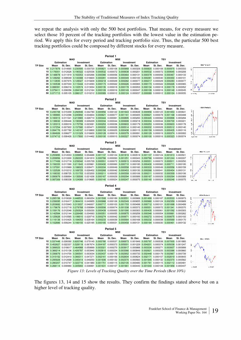
we repeat the analysis with only the 500 best portfolios. That means, for every measure we select those 10 percent of the tracking portfolios with the lowest value in the estimation pe-riod. We apply this for every period and tracking portfolio size. Thus, the particular 500 best tracking portfolios could be composed by different stocks for every measure.
TP Size Mean St. Dev. Mean St. Dev. Mean St. Dev. Mean St. Dev. Mean St. Dev. Mean St. Dev.
10 0.217879 0.014665 0.230585 0.030720 0.000821 0.000108 0.000968 0.000328 0.000820 0.000108 0.000975 0.000333
15 0.176001 0.012626 0.190322 0.025536 0.000532 0.000072 0.000638 0.000201 0.000532 0.000072 0.000645 0.000208
20 0.148878 0.011819 0.163353 0.020266 0.000380 0.000056 0.000464 0.000131 0.000379 0.000056 0.000467 0.000133
25 0.128262 0.009549 0.143388 0.018820 0.000281 0.000040 0.000349 0.000100 0.000281 0.000040 0.000350 0.000101
30 0.112835 0.007975 0.128327 0.015609 0.000218 0.000029 0.000282 0.000077 0.000217 0.000029 0.000283 0.000077
35 0.100538 0.007033 0.115444 0.014093 0.000173 0.000022 0.000226 0.000065 0.000173 0.000022 0.000226 0.000065
40 0.088391 0.006216 0.102574 0.013054 0.000135 0.000018 0.000178 0.000053 0.000134 0.000018 0.000178 0.000052
45 0.079411 0.006056 0.094165 0.012164 0.000109 0.000016 0.000149 0.000047 0.000109 0.000016 0.000148 0.000045
50 0.071713 0.005105 0.086127 0.010212 0.000089 0.000012 0.000124 0.000037 0.000089 0.000012 0.000124 0.000035
TP Size Mean St. Dev. Mean St. Dev. Mean St. Dev. Mean St. Dev. Mean St. Dev. Mean St. Dev.
10 0.235708 0.015359 0.292946 0.042780 0.000956 0.000122 0.001643 0.000638 0.000956 0.000123 0.001653 0.000641
15 0.189965 0.012296 0.245892 0.034604 0.000621 0.000077 0.001161 0.000405 0.000621 0.000078 0.001168 0.000408
20 0.160013 0.011541 0.213965 0.028710 0.000444 0.000061 0.000895 0.000293 0.000445 0.000062 0.000896 0.000294
25 0.138632 0.009446 0.190089 0.026229 0.000334 0.000044 0.000699 0.000218 0.000334 0.000044 0.000700 0.000221
30 0.120313 0.009316 0.170706 0.023081 0.000253 0.000036 0.000603 0.000179 0.000253 0.000036 0.000603 0.000178
35 0.107254 0.007922 0.157580 0.020471 0.000202 0.000028 0.000514 0.000140 0.000202 0.000028 0.000512 0.000140
40 0.094776 0.007782 0.143167 0.018800 0.000159 0.000025 0.000438 0.000115 0.000159 0.000025 0.000435 0.000116
45 0.084826 0.006677 0.131329 0.016600 0.000128 0.000019 0.000379 0.000091 0.000129 0.000019 0.000374 0.000093
50 0.074712 0.006426 0.117800 0.014462 0.000100 0.000015 0.000327 0.000074 0.000100 0.000016 0.000323 0.000074
TP Size Mean St. Dev. Mean St. Dev. Mean St. Dev. Mean St. Dev. Mean St. Dev. Mean St. Dev.
10 0.255895 0.014553 0.339953 0.054688 0.001137 0.000124 0.001819 0.000519 0.001137 0.000124 0.001813 0.000501
15 0.209956 0.013300 0.282220 0.041810 0.000766 0.000093 0.001251 0.000343 0.000766 0.000093 0.001244 0.000337
20 0.177406 0.012718 0.239342 0.035729 0.000551 0.000072 0.000915 0.000256 0.000551 0.000072 0.000911 0.000250
25 0.156333 0.011590 0.211643 0.029961 0.000430 0.000060 0.000710 0.000195 0.000430 0.000060 0.000711 0.000195
30 0.137091 0.010969 0.188023 0.028471 0.000334 0.000049 0.000558 0.000160 0.000333 0.000049 0.000556 0.000159
35 0.122526 0.010212 0.169725 0.026452 0.000268 0.000042 0.000453 0.000130 0.000268 0.000041 0.000454 0.000131
40 0.108332 0.008725 0.151703 0.023200 0.000211 0.000032 0.000359 0.000106 0.000211 0.000032 0.000359 0.000106
45 0.095879 0.008894 0.135506 0.021636 0.000167 0.000029 0.000294 0.000089 0.000167 0.000029 0.000294 0.000089
50 0.087309 0.008338 0.124089 0.019685 0.000140 0.000024 0.000247 0.000075 0.000140 0.000024 0.000246 0.000075
TP Size Mean St. Dev. Mean St. Dev. Mean St. Dev. Mean St. Dev. Mean St. Dev. Mean St. Dev.
10 0.295158 0.019026 0.448533 0.060254 0.001508 0.000189 0.003551 0.000988 0.001499 0.000187 0.003533 0.000973
15 0.239095 0.016417 0.364410 0.049955 0.000988 0.000126 0.002349 0.000655 0.000980 0.000124 0.002359 0.000669
20 0.203682 0.015943 0.313037 0.046007 0.000717 0.000103 0.001703 0.000498 0.000712 0.000101 0.001698 0.000499
25 0.179679 0.012718 0.279768 0.038984 0.000556 0.000074 0.001338 0.000372 0.000551 0.000072 0.001341 0.000370
30 0.159176 0.012048 0.250524 0.035030 0.000439 0.000063 0.001090 0.000303 0.000435 0.000061 0.001092 0.000303
35 0.142584 0.012144 0.226490 0.034063 0.000351 0.000055 0.000875 0.000258 0.000348 0.000054 0.000881 0.000262
40 0.125628 0.010565 0.199010 0.029716 0.000274 0.000042 0.000671 0.000193 0.000272 0.000042 0.000675 0.000193
45 0.116138 0.010425 0.184053 0.028164 0.000233 0.000039 0.000564 0.000168 0.000232 0.000038 0.000569 0.000170
50 0.102886 0.009244 0.166155 0.025185 0.000185 0.000031 0.000458 0.000131 0.000184 0.000030 0.000461 0.000132
TP Size Mean St. Dev. Mean St. Dev. Mean St. Dev. Mean St. Dev. Mean St. Dev. Mean St. Dev.
10 0.537448 0.026592 0.620746 0.079145 0.005780 0.000537 0.006973 0.001849 0.005797 0.000538 0.007005 0.001885
15 0.452627 0.022337 0.528118 0.067674 0.004187 0.000373 0.005001 0.001229 0.004201 0.000374 0.005038 0.001247
20 0.399023 0.018617 0.464988 0.059899 0.003321 0.000270 0.003917 0.000988 0.003334 0.000271 0.003937 0.000999
25 0.366214 0.015136 0.426787 0.053940 0.002810 0.000224 0.003366 0.000849 0.002821 0.000225 0.003386 0.000860
30 0.336879 0.014700 0.395541 0.053034 0.002437 0.000179 0.002952 0.000733 0.002448 0.000179 0.002967 0.000739
35 0.315152 0.012410 0.366311 0.047271 0.002161 0.000156 0.002604 0.000624 0.002171 0.000157 0.002619 0.000643
40 0.295928 0.012698 0.345414 0.049250 0.001936 0.000132 0.002370 0.000560 0.001945 0.000132 0.002370 0.000562
45 0.280207 0.010747 0.322716 0.041980 0.001751 0.000115 0.002105 0.000480 0.001761 0.000115 0.002112 0.000491
50 0.268114 0.009960 0.305993 0.038991 0.001631 0.000107 0.001961 0.000440 0.001640 0.000108 0.001958 0.000447
Estimation InvestmentEstimation Investment Estimation Investment
Estimation Investment
Period 5MAD MSE TEV
Estimation Investment Estimation Investment
Estimation Investment
Period 4MAD MSE TEV
Estimation Investment Estimation Investment
Period 3MAD MSE TEV
Investment Estimation Investment
Period 2
Estimation Investment Estimation
MAD MSE TEV
Estimation InvestmentInvestment Estimation Investment Estimation
Period 1MAD MSE TEV
Figure 13: Levels of Tracking Quality over the Time Periods (Best 10%)
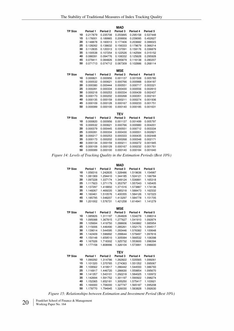
The figures 13, 14 and 15 show the results. They confirm the findings stated above but on a higher level of tracking quality.
The Stability of Traditional Measures of Index Tracking Quality
20 Frankfurt School of Finance & Management Working Paper No. 164
TP Size Period 1 Period 2 Period 3 Period 4 Period 5
10 0.217879 0.235708 0.255895 0.295158 0.537448
15 0.176001 0.189965 0.209956 0.239095 0.452627
20 0.148878 0.160013 0.177406 0.203682 0.399023
25 0.128262 0.138632 0.156333 0.179679 0.366214
30 0.112835 0.120313 0.137091 0.159176 0.336879
35 0.100538 0.107254 0.122526 0.142584 0.315152
40 0.088391 0.094776 0.108332 0.125628 0.295928
45 0.079411 0.084826 0.095879 0.116138 0.280207
50 0.071713 0.074712 0.087309 0.102886 0.268114
TP Size Period 1 Period 2 Period 3 Period 4 Period 5
10 0.000821 0.000956 0.001137 0.001508 0.005780
15 0.000532 0.000621 0.000766 0.000988 0.004187
20 0.000380 0.000444 0.000551 0.000717 0.003321
25 0.000281 0.000334 0.000430 0.000556 0.002810
30 0.000218 0.000253 0.000334 0.000439 0.002437
35 0.000173 0.000202 0.000268 0.000351 0.002161
40 0.000135 0.000159 0.000211 0.000274 0.001936
45 0.000109 0.000128 0.000167 0.000233 0.001751
50 0.000089 0.000100 0.000140 0.000185 0.001631
TP Size Period 1 Period 2 Period 3 Period 4 Period 5
10 0.000820 0.000956 0.001137 0.001499 0.005797
15 0.000532 0.000621 0.000766 0.000980 0.004201
20 0.000379 0.000445 0.000551 0.000712 0.003334
25 0.000281 0.000334 0.000430 0.000551 0.002821
30 0.000217 0.000253 0.000333 0.000435 0.002448
35 0.000173 0.000202 0.000268 0.000348 0.002171
40 0.000134 0.000159 0.000211 0.000272 0.001945
45 0.000109 0.000129 0.000167 0.000232 0.001761
50 0.000089 0.000100 0.000140 0.000184 0.001640
MAD
TEV
MSE
Figure 14: Levels of Tracking Quality in the Estimation Periods (Best 10%)
TP Size Period 1 Period 2 Period 3 Period 4 Period 5
10 1.058316 1.242835 1.328486 1.519636 1.154987
15 1.081369 1.294410 1.344185 1.524121 1.166784
20 1.097228 1.337174 1.349124 1.536891 1.165318
25 1.117923 1.371179 1.353797 1.557043 1.165405
30 1.137297 1.418850 1.371516 1.573887 1.174136
35 1.148267 1.469220 1.385218 1.588473 1.162332
40 1.160461 1.510576 1.400355 1.584126 1.167223
45 1.185795 1.548207 1.413297 1.584778 1.151705
50 1.201002 1.576731 1.421258 1.614941 1.141279
TP Size Period 1 Period 2 Period 3 Period 4 Period 5
10 1.085826 1.311197 1.264828 1.534278 1.098314
15 1.095088 1.367815 1.277627 1.541910 1.092874
20 1.105694 1.419750 1.288606 1.540882 1.085954
25 1.115006 1.446490 1.285261 1.552175 1.094517
30 1.139014 1.544595 1.293446 1.576382 1.100648
35 1.142409 1.596892 1.299644 1.579497 1.097816
40 1.150148 1.659510 1.305084 1.566532 1.106398
45 1.167026 1.718302 1.325732 1.553600 1.096394
50 1.177158 1.808996 1.326104 1.573991 1.096600
TP Size Period 1 Period 2 Period 3 Period 4 Period 5
10 1.090292 1.314786 1.262822 1.535565 1.099261
15 1.101320 1.370765 1.274363 1.551352 1.095067
20 1.109562 1.419917 1.286442 1.544550 1.086793
25 1.116917 1.446720 1.286630 1.559854 1.095670
30 1.141357 1.543101 1.292218 1.584025 1.100972
35 1.142694 1.591752 1.301197 1.590922 1.098274
40 1.152365 1.652181 1.305250 1.575417 1.103921
45 1.169300 1.706000 1.327747 1.565187 1.095208
50 1.178770 1.794945 1.326030 1.583828 1.092630
MAD
TEV
MSE
Figure 15: Relationships between Estimation and Investment Period (Best 10%)
The Stability of Traditional Measures of Index Tracking Quality
Frankfurt School of Finance & Management Working Paper No. 164 21
Compared to figure 12, figure 15 shows a more nebulous result. Here, we cannot even say in some periods which measure is the more stable. It is remarkable that the values are on a higher level in figure 15. That means that the stability of the best 10 percent is lower on aver-age than the stability over all portfolios. In other words, the discrepancy between estimation period and investment period is bigger on average.
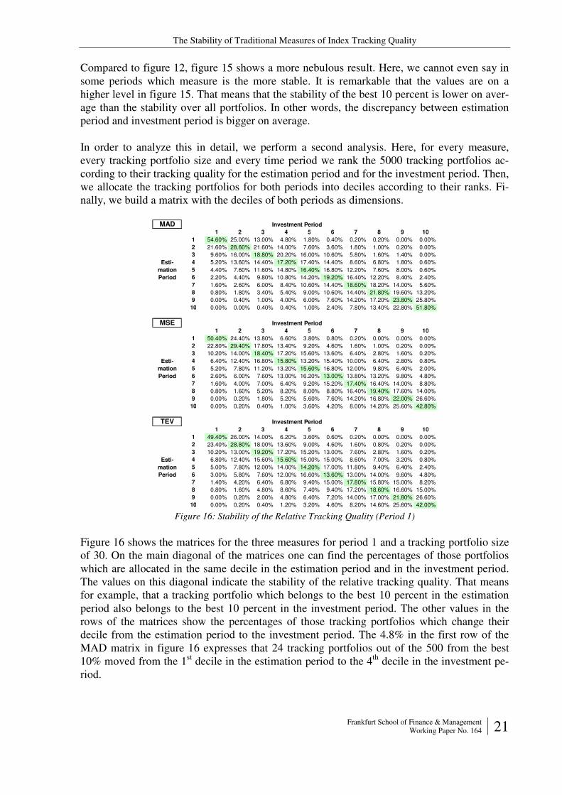
In order to analyze this in detail, we perform a second analysis. Here, for every measure, every tracking portfolio size and every time period we rank the 5000 tracking portfolios ac-cording to their tracking quality for the estimation period and for the investment period. Then, we allocate the tracking portfolios for both periods into deciles according to their ranks. Fi-nally, we build a matrix with the deciles of both periods as dimensions.
MAD1 2 3 4 5 6 7 8 9 10
1 54.60% 25.00% 13.00% 4.80% 1.80% 0.40% 0.20% 0.20% 0.00% 0.00%
2 21.60% 28.60% 21.60% 14.00% 7.60% 3.60% 1.80% 1.00% 0.20% 0.00%
3 9.60% 16.00% 18.80% 20.20% 16.00% 10.60% 5.80% 1.60% 1.40% 0.00%
4 5.20% 13.60% 14.40% 17.20% 17.40% 14.40% 8.60% 6.80% 1.80% 0.60%
5 4.40% 7.60% 11.60% 14.80% 16.40% 16.80% 12.20% 7.60% 8.00% 0.60%
6 2.20% 4.40% 9.80% 10.80% 14.20% 19.20% 16.40% 12.20% 8.40% 2.40%
7 1.60% 2.60% 6.00% 8.40% 10.60% 14.40% 18.60% 18.20% 14.00% 5.60%
8 0.80% 1.80% 3.40% 5.40% 9.00% 10.60% 14.40% 21.80% 19.60% 13.20%
9 0.00% 0.40% 1.00% 4.00% 6.00% 7.60% 14.20% 17.20% 23.80% 25.80%
10 0.00% 0.00% 0.40% 0.40% 1.00% 2.40% 7.80% 13.40% 22.80% 51.80%
MSE1 2 3 4 5 6 7 8 9 10
1 50.40% 24.40% 13.80% 6.60% 3.80% 0.80% 0.20% 0.00% 0.00% 0.00%
2 22.80% 29.40% 17.80% 13.40% 9.20% 4.60% 1.60% 1.00% 0.20% 0.00%
3 10.20% 14.00% 18.40% 17.20% 15.60% 13.60% 6.40% 2.80% 1.60% 0.20%
4 6.40% 12.40% 16.80% 15.80% 13.20% 15.40% 10.00% 6.40% 2.80% 0.80%
5 5.20% 7.80% 11.20% 13.20% 15.60% 16.80% 12.00% 9.80% 6.40% 2.00%
6 2.60% 6.00% 7.60% 13.00% 16.20% 13.00% 13.80% 13.20% 9.80% 4.80%
7 1.60% 4.00% 7.00% 6.40% 9.20% 15.20% 17.40% 16.40% 14.00% 8.80%
8 0.80% 1.60% 5.20% 8.20% 8.00% 8.80% 16.40% 19.40% 17.60% 14.00%
9 0.00% 0.20% 1.80% 5.20% 5.60% 7.60% 14.20% 16.80% 22.00% 26.60%
10 0.00% 0.20% 0.40% 1.00% 3.60% 4.20% 8.00% 14.20% 25.60% 42.80%
TEV1 2 3 4 5 6 7 8 9 10
1 49.40% 26.00% 14.00% 6.20% 3.60% 0.60% 0.20% 0.00% 0.00% 0.00%
2 23.40% 28.80% 18.00% 13.60% 9.00% 4.60% 1.60% 0.80% 0.20% 0.00%
3 10.20% 13.00% 19.20% 17.20% 15.20% 13.00% 7.60% 2.80% 1.60% 0.20%
4 6.80% 12.40% 15.60% 15.60% 15.00% 15.00% 8.60% 7.00% 3.20% 0.80%
5 5.00% 7.80% 12.00% 14.00% 14.20% 17.00% 11.80% 9.40% 6.40% 2.40%
6 3.00% 5.80% 7.60% 12.00% 16.60% 13.60% 13.00% 14.00% 9.60% 4.80%
7 1.40% 4.20% 6.40% 6.80% 9.40% 15.00% 17.80% 15.80% 15.00% 8.20%
8 0.80% 1.60% 4.80% 8.60% 7.40% 9.40% 17.20% 18.60% 16.60% 15.00%
9 0.00% 0.20% 2.00% 4.80% 6.40% 7.20% 14.00% 17.00% 21.80% 26.60%
10 0.00% 0.20% 0.40% 1.20% 3.20% 4.60% 8.20% 14.60% 25.60% 42.00%
Investment Period
Esti-
mation
Period
Investment Period
Investment Period
Esti-
mation
Period
Esti-
mation
Period
Figure 16: Stability of the Relative Tracking Quality (Period 1)
Figure 16 shows the matrices for the three measures for period 1 and a tracking portfolio size of 30. On the main diagonal of the matrices one can find the percentages of those portfolios which are allocated in the same decile in the estimation period and in the investment period. The values on this diagonal indicate the stability of the relative tracking quality. That means for example, that a tracking portfolio which belongs to the best 10 percent in the estimation period also belongs to the best 10 percent in the investment period. The other values in the rows of the matrices show the percentages of those tracking portfolios which change their decile from the estimation period to the investment period. The 4.8% in the first row of the MAD matrix in figure 16 expresses that 24 tracking portfolios out of the 500 from the best 10% moved from the 1st decile in the estimation period to the 4th decile in the investment pe-riod.
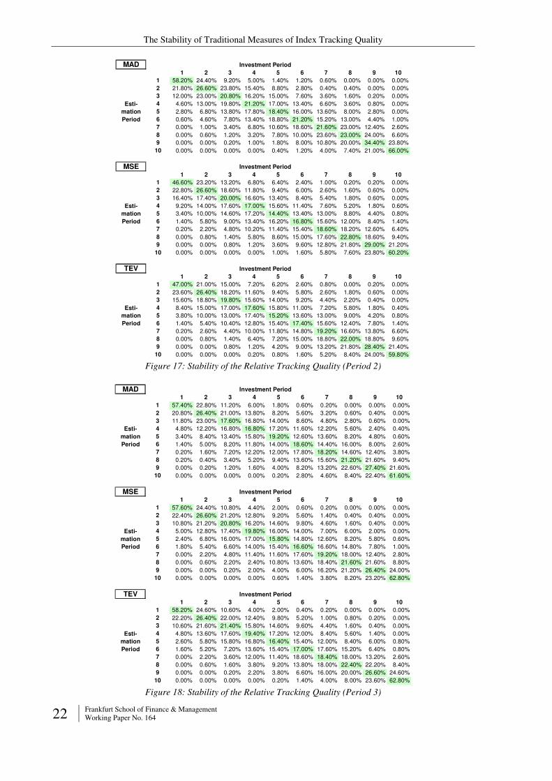
The Stability of Traditional Measures of Index Tracking Quality
22 Frankfurt School of Finance & Management Working Paper No. 164
MAD1 2 3 4 5 6 7 8 9 10
1 58.20% 24.40% 9.20% 5.00% 1.40% 1.20% 0.60% 0.00% 0.00% 0.00%
2 21.80% 26.60% 23.80% 15.40% 8.80% 2.80% 0.40% 0.40% 0.00% 0.00%
3 12.00% 23.00% 20.80% 16.20% 15.00% 7.60% 3.60% 1.60% 0.20% 0.00%
4 4.60% 13.00% 19.80% 21.20% 17.00% 13.40% 6.60% 3.60% 0.80% 0.00%
5 2.80% 6.80% 13.80% 17.80% 18.40% 16.00% 13.60% 8.00% 2.80% 0.00%
6 0.60% 4.60% 7.80% 13.40% 18.80% 21.20% 15.20% 13.00% 4.40% 1.00%
7 0.00% 1.00% 3.40% 6.80% 10.60% 18.60% 21.60% 23.00% 12.40% 2.60%
8 0.00% 0.60% 1.20% 3.20% 7.80% 10.00% 23.60% 23.00% 24.00% 6.60%
9 0.00% 0.00% 0.20% 1.00% 1.80% 8.00% 10.80% 20.00% 34.40% 23.80%
10 0.00% 0.00% 0.00% 0.00% 0.40% 1.20% 4.00% 7.40% 21.00% 66.00%
MSE1 2 3 4 5 6 7 8 9 10
1 46.60% 23.20% 13.20% 6.80% 6.40% 2.40% 1.00% 0.20% 0.20% 0.00%
2 22.80% 26.60% 18.60% 11.80% 9.40% 6.00% 2.60% 1.60% 0.60% 0.00%
3 16.40% 17.40% 20.00% 16.60% 13.40% 8.40% 5.40% 1.80% 0.60% 0.00%
4 9.20% 14.00% 17.60% 17.00% 15.60% 11.40% 7.60% 5.20% 1.80% 0.60%
5 3.40% 10.00% 14.60% 17.20% 14.40% 13.40% 13.00% 8.80% 4.40% 0.80%
6 1.40% 5.80% 9.00% 13.40% 16.20% 16.80% 15.60% 12.00% 8.40% 1.40%
7 0.20% 2.20% 4.80% 10.20% 11.40% 15.40% 18.60% 18.20% 12.60% 6.40%
8 0.00% 0.80% 1.40% 5.80% 8.60% 15.00% 17.60% 22.80% 18.60% 9.40%
9 0.00% 0.00% 0.80% 1.20% 3.60% 9.60% 12.80% 21.80% 29.00% 21.20%
10 0.00% 0.00% 0.00% 0.00% 1.00% 1.60% 5.80% 7.60% 23.80% 60.20%
TEV1 2 3 4 5 6 7 8 9 10
1 47.00% 21.00% 15.00% 7.20% 6.20% 2.60% 0.80% 0.00% 0.20% 0.00%
2 23.60% 26.40% 18.20% 11.60% 9.40% 5.80% 2.60% 1.80% 0.60% 0.00%
3 15.60% 18.80% 19.80% 15.60% 14.00% 9.20% 4.40% 2.20% 0.40% 0.00%
4 8.40% 15.00% 17.00% 17.60% 15.80% 11.00% 7.20% 5.80% 1.80% 0.40%
5 3.80% 10.00% 13.00% 17.40% 15.20% 13.60% 13.00% 9.00% 4.20% 0.80%
6 1.40% 5.40% 10.40% 12.80% 15.40% 17.40% 15.60% 12.40% 7.80% 1.40%
7 0.20% 2.60% 4.40% 10.00% 11.80% 14.80% 19.20% 16.60% 13.80% 6.60%
8 0.00% 0.80% 1.40% 6.40% 7.20% 15.00% 18.80% 22.00% 18.80% 9.60%
9 0.00% 0.00% 0.80% 1.20% 4.20% 9.00% 13.20% 21.80% 28.40% 21.40%
10 0.00% 0.00% 0.00% 0.20% 0.80% 1.60% 5.20% 8.40% 24.00% 59.80%
Investment Period
Esti-
mation
Period
Investment Period
Investment Period
Esti-
mation
Period
Esti-
mation
Period
Figure 17: Stability of the Relative Tracking Quality (Period 2)
MAD1 2 3 4 5 6 7 8 9 10
1 57.40% 22.80% 11.20% 6.00% 1.80% 0.60% 0.20% 0.00% 0.00% 0.00%
2 20.80% 26.40% 21.00% 13.80% 8.20% 5.60% 3.20% 0.60% 0.40% 0.00%
3 11.80% 23.00% 17.60% 16.80% 14.00% 8.60% 4.80% 2.80% 0.60% 0.00%
4 4.80% 12.20% 16.80% 16.80% 17.20% 11.60% 12.20% 5.60% 2.40% 0.40%
5 3.40% 8.40% 13.40% 15.80% 19.20% 12.60% 13.60% 8.20% 4.80% 0.60%
6 1.40% 5.00% 8.20% 11.80% 14.00% 18.60% 14.40% 16.00% 8.00% 2.60%
7 0.20% 1.60% 7.20% 12.20% 12.00% 17.80% 18.20% 14.60% 12.40% 3.80%
8 0.20% 0.40% 3.40% 5.20% 9.40% 13.60% 15.60% 21.20% 21.60% 9.40%
9 0.00% 0.20% 1.20% 1.60% 4.00% 8.20% 13.20% 22.60% 27.40% 21.60%
10 0.00% 0.00% 0.00% 0.00% 0.20% 2.80% 4.60% 8.40% 22.40% 61.60%
MSE1 2 3 4 5 6 7 8 9 10
1 57.60% 24.40% 10.80% 4.40% 2.00% 0.60% 0.20% 0.00% 0.00% 0.00%
2 22.40% 26.60% 21.20% 12.80% 9.20% 5.60% 1.40% 0.40% 0.40% 0.00%
3 10.80% 21.20% 20.80% 16.20% 14.60% 9.80% 4.60% 1.60% 0.40% 0.00%
4 5.00% 12.80% 17.40% 19.80% 16.00% 14.00% 7.00% 6.00% 2.00% 0.00%
5 2.40% 6.80% 16.00% 17.00% 15.80% 14.80% 12.60% 8.20% 5.80% 0.60%
6 1.80% 5.40% 6.60% 14.00% 15.40% 16.60% 16.60% 14.80% 7.80% 1.00%
7 0.00% 2.20% 4.80% 11.40% 11.60% 17.60% 19.20% 18.00% 12.40% 2.80%
8 0.00% 0.60% 2.20% 2.40% 10.80% 13.60% 18.40% 21.60% 21.60% 8.80%
9 0.00% 0.00% 0.20% 2.00% 4.00% 6.00% 16.20% 21.20% 26.40% 24.00%
10 0.00% 0.00% 0.00% 0.00% 0.60% 1.40% 3.80% 8.20% 23.20% 62.80%
TEV1 2 3 4 5 6 7 8 9 10
1 58.20% 24.60% 10.60% 4.00% 2.00% 0.40% 0.20% 0.00% 0.00% 0.00%
2 22.20% 26.40% 22.00% 12.40% 9.80% 5.20% 1.00% 0.80% 0.20% 0.00%
3 10.60% 21.60% 21.40% 15.80% 14.60% 9.60% 4.40% 1.60% 0.40% 0.00%
4 4.80% 13.60% 17.60% 19.40% 17.20% 12.00% 8.40% 5.60% 1.40% 0.00%
5 2.60% 5.80% 15.80% 16.80% 16.40% 15.40% 12.00% 8.40% 6.00% 0.80%
6 1.60% 5.20% 7.20% 13.60% 15.40% 17.00% 17.60% 15.20% 6.40% 0.80%
7 0.00% 2.20% 3.60% 12.00% 11.40% 18.60% 18.40% 18.00% 13.20% 2.60%
8 0.00% 0.60% 1.60% 3.80% 9.20% 13.80% 18.00% 22.40% 22.20% 8.40%
9 0.00% 0.00% 0.20% 2.20% 3.80% 6.60% 16.00% 20.00% 26.60% 24.60%
10 0.00% 0.00% 0.00% 0.00% 0.20% 1.40% 4.00% 8.00% 23.60% 62.80%
Investment Period
Esti-
mation
Period
Investment Period
Investment Period
Esti-
mation
Period
Esti-
mation
Period
Figure 18: Stability of the Relative Tracking Quality (Period 3)
The Stability of Traditional Measures of Index Tracking Quality
Frankfurt School of Finance & Management Working Paper No. 164 23
MAD1 2 3 4 5 6 7 8 9 10
1 58.40% 23.80% 11.20% 4.80% 1.00% 0.60% 0.20% 0.00% 0.00% 0.00%
2 21.60% 30.20% 20.80% 13.60% 9.20% 2.60% 1.60% 0.40% 0.00% 0.00%
3 9.40% 20.80% 21.80% 17.00% 13.00% 10.60% 4.40% 2.20% 0.80% 0.00%
4 5.60% 13.40% 17.00% 18.20% 17.40% 12.80% 9.00% 4.60% 2.00% 0.00%
5 3.00% 5.80% 13.00% 17.20% 17.80% 16.20% 13.00% 9.40% 4.00% 0.60%
6 1.00% 3.40% 9.00% 13.80% 15.40% 18.20% 15.60% 12.20% 9.40% 2.00%
7 0.60% 1.60% 4.40% 8.80% 10.80% 18.80% 17.80% 20.80% 12.80% 3.60%
8 0.40% 0.60% 1.40% 3.80% 10.40% 11.20% 19.20% 19.80% 23.40% 9.80%
9 0.00% 0.20% 0.80% 2.40% 4.00% 7.60% 14.40% 22.00% 25.60% 23.00%
10 0.00% 0.20% 0.60% 0.40% 1.00% 1.40% 4.80% 8.60% 22.00% 61.00%
MSE1 2 3 4 5 6 7 8 9 10
1 58.20% 23.60% 12.20% 4.20% 1.00% 0.80% 0.00% 0.00% 0.00% 0.00%
2 24.40% 26.60% 25.60% 12.00% 7.40% 2.60% 1.00% 0.40% 0.00% 0.00%
3 9.20% 20.20% 20.00% 20.00% 13.80% 8.80% 5.40% 2.40% 0.20% 0.00%
4 4.80% 13.20% 20.00% 17.80% 18.80% 11.20% 7.80% 5.00% 1.40% 0.00%
5 2.00% 9.00% 9.80% 18.80% 17.60% 18.00% 13.80% 7.60% 3.00% 0.40%
6 1.00% 4.20% 7.00% 13.20% 16.20% 17.60% 16.80% 14.60% 8.60% 0.80%
7 0.40% 2.20% 3.20% 8.40% 12.60% 18.20% 22.80% 19.00% 9.40% 3.80%
8 0.00% 0.60% 1.80% 4.40% 8.80% 13.60% 16.20% 22.80% 23.80% 8.00%
9 0.00% 0.00% 0.40% 1.20% 3.20% 7.60% 13.60% 21.60% 30.00% 22.40%
10 0.00% 0.40% 0.00% 0.00% 0.60% 1.60% 2.60% 6.60% 23.60% 64.60%
TEV1 2 3 4 5 6 7 8 9 10
1 57.20% 23.60% 13.40% 3.60% 1.20% 0.80% 0.20% 0.00% 0.00% 0.00%
2 24.20% 27.40% 24.00% 12.80% 7.60% 2.40% 1.20% 0.40% 0.00% 0.00%
3 9.40% 20.60% 21.80% 18.60% 13.20% 8.40% 5.20% 2.20% 0.60% 0.00%
4 5.60% 13.00% 18.80% 19.80% 18.00% 11.80% 6.80% 4.40% 1.80% 0.00%
5 2.20% 7.20% 9.60% 17.80% 17.80% 19.40% 14.20% 7.80% 3.60% 0.40%
6 0.60% 5.40% 7.80% 13.40% 16.60% 16.60% 17.60% 13.80% 7.40% 0.80%
7 0.60% 1.40% 3.20% 9.00% 13.80% 17.00% 19.60% 20.60% 10.60% 4.20%
8 0.20% 0.80% 1.20% 4.60% 8.20% 13.20% 19.20% 23.80% 21.60% 7.20%
9 0.00% 0.20% 0.20% 0.40% 3.20% 9.00% 13.80% 20.00% 30.40% 22.80%
10 0.00% 0.40% 0.00% 0.00% 0.40% 1.40% 2.20% 7.00% 24.00% 64.60%
Investment Period
Esti-
mation
Period
Investment Period
Investment Period
Esti-
mation
Period
Esti-
mation
Period
Figure 19: Stability of the Relative Tracking Quality (Period 4)
MAD1 2 3 4 5 6 7 8 9 10
1 45.80% 21.80% 16.40% 6.80% 3.60% 3.00% 1.00% 0.80% 0.60% 0.20%
2 25.80% 22.20% 17.20% 11.60% 8.00% 8.20% 3.00% 1.60% 2.00% 0.40%
3 12.40% 18.00% 16.80% 16.00% 11.20% 11.20% 7.60% 4.80% 1.60% 0.40%
4 7.80% 13.60% 15.20% 14.40% 14.40% 12.60% 9.40% 7.40% 3.80% 1.40%
5 4.40% 10.20% 12.20% 14.40% 11.20% 13.00% 11.40% 12.80% 6.80% 3.60%
6 2.20% 6.00% 10.00% 11.60% 16.60% 13.80% 14.00% 11.00% 10.20% 4.60%
7 0.60% 4.00% 4.60% 11.20% 14.80% 14.60% 13.00% 13.40% 14.20% 9.60%
8 0.60% 3.00% 4.80% 6.60% 10.00% 11.00% 17.80% 19.60% 17.40% 9.20%
9 0.20% 1.20% 2.40% 5.20% 8.00% 9.40% 13.60% 18.00% 20.40% 21.60%
10 0.20% 0.00% 0.40% 2.20% 2.20% 3.20% 9.20% 10.60% 23.00% 49.00%
MSE1 2 3 4 5 6 7 8 9 10
1 41.80% 24.60% 13.00% 10.00% 4.40% 1.80% 2.00% 1.60% 0.80% 0.00%
2 24.40% 20.00% 17.60% 12.80% 10.00% 5.40% 4.80% 2.80% 1.80% 0.40%
3 16.00% 17.60% 16.40% 12.60% 11.20% 12.60% 6.60% 4.00% 2.40% 0.60%
4 9.00% 14.20% 14.20% 14.20% 15.40% 9.00% 11.40% 6.00% 4.80% 1.80%
5 5.00% 10.80% 10.80% 15.60% 13.00% 13.80% 10.00% 10.60% 6.60% 3.80%
6 2.60% 6.00% 10.80% 12.60% 14.40% 12.80% 13.80% 11.40% 10.60% 5.00%
7 1.00% 4.20% 8.20% 11.00% 11.80% 14.40% 13.80% 16.60% 11.00% 8.00%
8 0.00% 1.80% 4.40% 5.20% 10.80% 14.40% 14.80% 16.60% 20.00% 12.00%
9 0.20% 0.80% 3.80% 4.40% 6.40% 12.00% 13.60% 17.20% 17.80% 23.80%
10 0.00% 0.00% 0.80% 1.60% 2.60% 3.80% 9.20% 13.20% 24.20% 44.60%
TEV1 2 3 4 5 6 7 8 9 10
1 41.40% 25.00% 12.80% 10.40% 3.60% 2.40% 2.00% 1.60% 0.80% 0.00%
2 24.60% 19.60% 18.20% 11.60% 10.80% 5.20% 5.00% 2.80% 1.80% 0.40%
3 15.40% 18.20% 16.60% 12.80% 10.60% 12.60% 6.60% 4.00% 2.40% 0.80%
4 9.20% 13.00% 15.60% 14.40% 14.80% 10.20% 9.80% 7.00% 4.40% 1.60%
5 5.20% 10.80% 10.20% 15.20% 13.20% 12.80% 11.00% 9.80% 8.20% 3.60%
6 2.60% 6.80% 10.00% 12.80% 14.00% 13.80% 13.60% 12.00% 9.60% 4.80%
7 1.00% 4.00% 7.80% 10.60% 13.20% 14.40% 13.80% 15.20% 11.60% 8.40%
8 0.40% 1.80% 4.20% 5.80% 11.20% 13.40% 14.60% 17.00% 20.00% 11.60%
9 0.20% 0.80% 3.60% 4.80% 6.60% 11.60% 14.20% 16.80% 18.20% 23.20%
10 0.00% 0.00% 1.00% 1.60% 2.00% 3.60% 9.40% 13.80% 23.00% 45.60%
Investment Period
Esti-
mation
Period
Investment Period
Investment Period
Esti-
mation
Period
Esti-
mation
Period
Figure 20: Stability of the Relative Tracking Quality (Period 5)
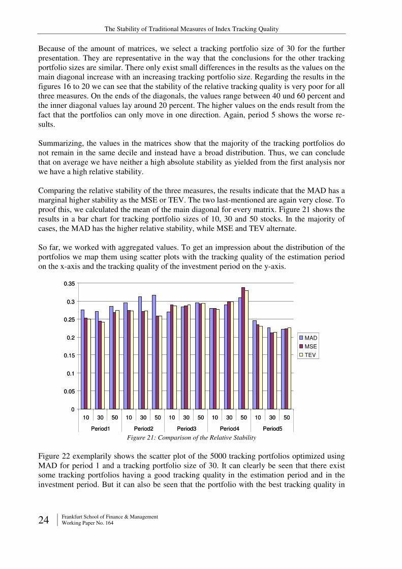
The Stability of Traditional Measures of Index Tracking Quality
24 Frankfurt School of Finance & Management Working Paper No. 164
Because of the amount of matrices, we select a tracking portfolio size of 30 for the further presentation. They are representative in the way that the conclusions for the other tracking portfolio sizes are similar. There only exist small differences in the results as the values on the main diagonal increase with an increasing tracking portfolio size. Regarding the results in the figures 16 to 20 we can see that the stability of the relative tracking quality is very poor for all three measures. On the ends of the diagonals, the values range between 40 und 60 percent and the inner diagonal values lay around 20 percent. The higher values on the ends result from the fact that the portfolios can only move in one direction. Again, period 5 shows the worse re-sults.
Summarizing, the values in the matrices show that the majority of the tracking portfolios do not remain in the same decile and instead have a broad distribution. Thus, we can conclude that on average we have neither a high absolute stability as yielded from the first analysis nor we have a high relative stability.
Comparing the relative stability of the three measures, the results indicate that the MAD has a marginal higher stability as the MSE or TEV. The two last-mentioned are again very close. To proof this, we calculated the mean of the main diagonal for every matrix. Figure 21 shows the results in a bar chart for tracking portfolio sizes of 10, 30 and 50 stocks. In the majority of cases, the MAD has the higher relative stability, while MSE and TEV alternate.
So far, we worked with aggregated values. To get an impression about the distribution of the portfolios we map them using scatter plots with the tracking quality of the estimation period on the x-axis and the tracking quality of the investment period on the y-axis.
0
0.05
0.1
0.15
0.2
0.25
0.3
0.35
10 30 50 10 30 50 10 30 50 10 30 50 10 30 50
Period1 Period2 Period3 Period4 Period5
MAD
MSE
TEV
0
0.05
0.1
0.15
0.2
0.25
0.3
0.35
10 30 50 10 30 50 10 30 50 10 30 50 10 30 50
Period1 Period2 Period3 Period4 Period5
MAD
MSE
TEV
Figure 21: Comparison of the Relative Stability
Figure 22 exemplarily shows the scatter plot of the 5000 tracking portfolios optimized using MAD for period 1 and a tracking portfolio size of 30. It can clearly be seen that there exist some tracking portfolios having a good tracking quality in the estimation period and in the investment period. But it can also be seen that the portfolio with the best tracking quality in
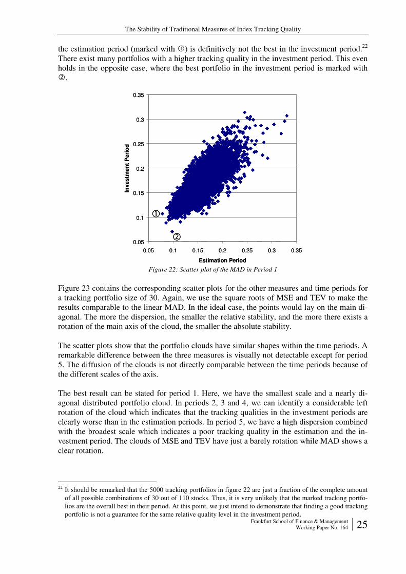
The Stability of Traditional Measures of Index Tracking Quality
Frankfurt School of Finance & Management Working Paper No. 164 25
the estimation period (marked with �) is definitively not the best in the investment period.22 There exist many portfolios with a higher tracking quality in the investment period. This even holds in the opposite case, where the best portfolio in the investment period is marked with �.
�
�0.05
0.1
0.15
0.2
0.25
0.3
0.35
0.05 0.1 0.15 0.2 0.25 0.3 0.35
Estimation Period
Inv
es
tme
nt
Peri
od
�
�0.05
0.1
0.15
0.2
0.25
0.3
0.35
0.05 0.1 0.15 0.2 0.25 0.3 0.35
Estimation Period
Inv
es
tme
nt
Peri
od
Figure 22: Scatter plot of the MAD in Period 1
Figure 23 contains the corresponding scatter plots for the other measures and time periods for a tracking portfolio size of 30. Again, we use the square roots of MSE and TEV to make the results comparable to the linear MAD. In the ideal case, the points would lay on the main di-agonal. The more the dispersion, the smaller the relative stability, and the more there exists a rotation of the main axis of the cloud, the smaller the absolute stability.
The scatter plots show that the portfolio clouds have similar shapes within the time periods. A remarkable difference between the three measures is visually not detectable except for period 5. The diffusion of the clouds is not directly comparable between the time periods because of the different scales of the axis.
The best result can be stated for period 1. Here, we have the smallest scale and a nearly di-agonal distributed portfolio cloud. In periods 2, 3 and 4, we can identify a considerable left rotation of the cloud which indicates that the tracking qualities in the investment periods are clearly worse than in the estimation periods. In period 5, we have a high dispersion combined with the broadest scale which indicates a poor tracking quality in the estimation and the in-vestment period. The clouds of MSE and TEV have just a barely rotation while MAD shows a clear rotation.
22 It should be remarked that the 5000 tracking portfolios in figure 22 are just a fraction of the complete amount
of all possible combinations of 30 out of 110 stocks. Thus, it is very unlikely that the marked tracking portfo-lios are the overall best in their period. At this point, we just intend to demonstrate that finding a good tracking portfolio is not a guarantee for the same relative quality level in the investment period.
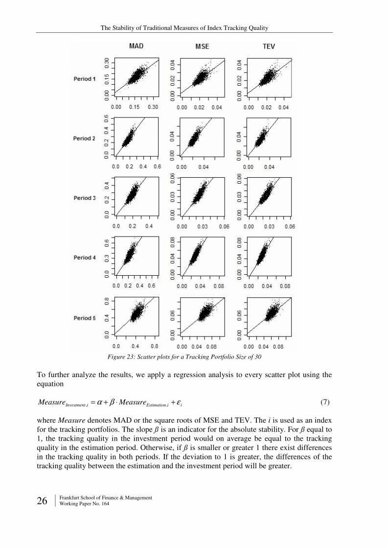
The Stability of Traditional Measures of Index Tracking Quality
26 Frankfurt School of Finance & Management Working Paper No. 164
Figure 23: Scatter plots for a Tracking Portfolio Size of 30
To further analyze the results, we apply a regression analysis to every scatter plot using the equation
ii,Estimationi,Investment MeasureMeasure εβα +⋅+= (7)
where Measure denotes MAD or the square roots of MSE and TEV. The i is used as an index for the tracking portfolios. The slope ß is an indicator for the absolute stability. For ß equal to 1, the tracking quality in the investment period would on average be equal to the tracking quality in the estimation period. Otherwise, if ß is smaller or greater 1 there exist differences in the tracking quality in both periods. If the deviation to 1 is greater, the differences of the tracking quality between the estimation and the investment period will be greater.
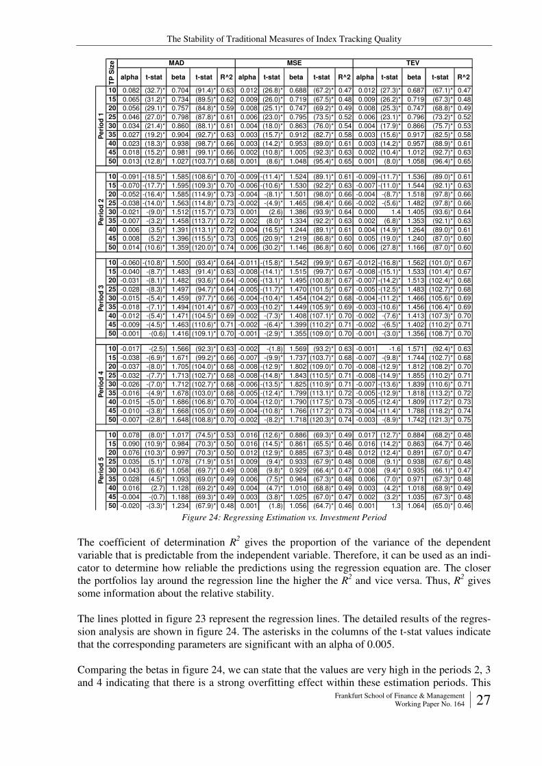
The Stability of Traditional Measures of Index Tracking Quality
Frankfurt School of Finance & Management Working Paper No. 164 27
alpha t-stat beta t-stat R^2 alpha t-stat beta t-stat R^2 alpha t-stat beta t-stat R^2
10 0.082 (32.7)* 0.704 (91.4)* 0.63 0.012 (26.8)* 0.688 (67.2)* 0.47 0.012 (27.3)* 0.687 (67.1)* 0.47
15 0.065 (31.2)* 0.734 (89.5)* 0.62 0.009 (26.0)* 0.719 (67.5)* 0.48 0.009 (26.2)* 0.719 (67.3)* 0.48
20 0.056 (29.1)* 0.757 (84.8)* 0.59 0.008 (25.1)* 0.747 (69.2)* 0.49 0.008 (25.3)* 0.747 (68.8)* 0.49
25 0.046 (27.0)* 0.798 (87.8)* 0.61 0.006 (23.0)* 0.795 (73.5)* 0.52 0.006 (23.1)* 0.796 (73.2)* 0.52
30 0.034 (21.4)* 0.860 (88.1)* 0.61 0.004 (18.0)* 0.863 (76.0)* 0.54 0.004 (17.9)* 0.866 (75.7)* 0.53
35 0.027 (19.2)* 0.904 (92.7)* 0.63 0.003 (15.7)* 0.912 (82.7)* 0.58 0.003 (15.6)* 0.917 (82.5)* 0.58
40 0.023 (18.3)* 0.938 (98.7)* 0.66 0.003 (14.2)* 0.953 (89.0)* 0.61 0.003 (14.2)* 0.957 (88.9)* 0.61
45 0.018 (15.2)* 0.981 (99.1)* 0.66 0.002 (10.8)* 1.005 (92.3)* 0.63 0.002 (10.4)* 1.012 (92.7)* 0.63
50 0.013 (12.8)* 1.027 (103.7)* 0.68 0.001 (8.6)* 1.048 (95.4)* 0.65 0.001 (8.0)* 1.058 (96.4)* 0.65
10 -0.091 -(18.5)* 1.585 (108.6)* 0.70 -0.009 -(11.4)* 1.524 (89.1)* 0.61 -0.009 -(11.7)* 1.536 (89.0)* 0.61
15 -0.070 -(17.7)* 1.595 (109.3)* 0.70 -0.006 -(10.6)* 1.530 (92.2)* 0.63 -0.007 -(11.0)* 1.544 (92.1)* 0.63
20 -0.052 -(16.4)* 1.585 (114.9)* 0.73 -0.004 -(8.1)* 1.501 (98.0)* 0.66 -0.004 -(8.7)* 1.518 (97.8)* 0.66
25 -0.038 -(14.0)* 1.563 (114.8)* 0.73 -0.002 -(4.9)* 1.465 (98.4)* 0.66 -0.002 -(5.6)* 1.482 (97.8)* 0.66
30 -0.021 -(9.0)* 1.512 (115.7)* 0.73 0.001 (2.6) 1.386 (93.9)* 0.64 0.000 1.4 1.405 (93.6)* 0.64
35 -0.007 -(3.2)* 1.458 (113.7)* 0.72 0.002 (8.0)* 1.334 (92.2)* 0.63 0.002 (6.8)* 1.353 (92.1)* 0.63
40 0.006 (3.5)* 1.391 (113.1)* 0.72 0.004 (16.5)* 1.244 (89.1)* 0.61 0.004 (14.9)* 1.264 (89.0)* 0.61
45 0.008 (5.2)* 1.396 (115.5)* 0.73 0.005 (20.9)* 1.219 (86.8)* 0.60 0.005 (19.0)* 1.240 (87.0)* 0.60
50 0.014 (10.6)* 1.359 (120.0)* 0.74 0.006 (30.2)* 1.146 (86.8)* 0.60 0.006 (27.8)* 1.166 (87.0)* 0.60
10 -0.060 -(10.8)* 1.500 (93.4)* 0.64 -0.011 -(15.8)* 1.542 (99.9)* 0.67 -0.012 -(16.8)* 1.562 (101.0)* 0.67
15 -0.040 -(8.7)* 1.483 (91.4)* 0.63 -0.008 -(14.1)* 1.515 (99.7)* 0.67 -0.008 -(15.1)* 1.533 (101.4)* 0.67
20 -0.031 -(8.1)* 1.482 (93.6)* 0.64 -0.006 -(13.1)* 1.495 (100.8)* 0.67 -0.007 -(14.2)* 1.513 (102.4)* 0.68
25 -0.028 -(8.3)* 1.497 (94.7)* 0.64 -0.005 -(11.7)* 1.470 (101.5)* 0.67 -0.005 -(12.5)* 1.483 (102.7)* 0.68
30 -0.015 -(5.4)* 1.459 (97.7)* 0.66 -0.004 -(10.4)* 1.454 (104.2)* 0.68 -0.004 -(11.2)* 1.466 (105.6)* 0.69
35 -0.018 -(7.1)* 1.494 (101.4)* 0.67 -0.003 -(10.2)* 1.449 (105.9)* 0.69 -0.003 -(10.6)* 1.456 (106.4)* 0.69
40 -0.012 -(5.4)* 1.471 (104.5)* 0.69 -0.002 -(7.3)* 1.408 (107.1)* 0.70 -0.002 -(7.6)* 1.413 (107.3)* 0.70
45 -0.009 -(4.5)* 1.463 (110.6)* 0.71 -0.002 -(6.4)* 1.399 (110.2)* 0.71 -0.002 -(6.5)* 1.402 (110.2)* 0.71
50 -0.001 -(0.6) 1.416 (109.1)* 0.70 -0.001 -(2.9)* 1.355 (109.0)* 0.70 -0.001 -(3.0)* 1.356 (108.7)* 0.70
10 -0.017 -(2.5) 1.566 (92.3)* 0.63 -0.002 -(1.8) 1.569 (93.2)* 0.63 -0.001 -1.6 1.571 (92.4)* 0.63
15 -0.038 -(6.9)* 1.671 (99.2)* 0.66 -0.007 -(9.9)* 1.737 (103.7)* 0.68 -0.007 -(9.8)* 1.744 (102.7)* 0.68
20 -0.037 -(8.0)* 1.705 (104.0)* 0.68 -0.008 -(12.9)* 1.802 (109.0)* 0.70 -0.008 -(12.9)* 1.812 (108.2)* 0.70
25 -0.032 -(7.7)* 1.713 (102.7)* 0.68 -0.008 -(14.8)* 1.843 (110.5)* 0.71 -0.008 -(14.9)* 1.855 (110.2)* 0.71
30 -0.026 -(7.0)* 1.712 (102.7)* 0.68 -0.006 -(13.5)* 1.825 (110.9)* 0.71 -0.007 -(13.6)* 1.839 (110.6)* 0.71
35 -0.016 -(4.9)* 1.678 (103.0)* 0.68 -0.005 -(12.4)* 1.799 (113.1)* 0.72 -0.005 -(12.9)* 1.818 (113.2)* 0.72
40 -0.015 -(5.0)* 1.686 (106.8)* 0.70 -0.004 -(12.0)* 1.790 (117.5)* 0.73 -0.005 -(12.4)* 1.809 (117.2)* 0.73
45 -0.010 -(3.8)* 1.668 (105.0)* 0.69 -0.004 -(10.8)* 1.766 (117.2)* 0.73 -0.004 -(11.4)* 1.788 (118.2)* 0.74
50 -0.007 -(2.8)* 1.648 (108.8)* 0.70 -0.002 -(8.2)* 1.718 (120.3)* 0.74 -0.003 -(8.9)* 1.742 (121.3)* 0.75
10 0.078 (8.0)* 1.017 (74.5)* 0.53 0.016 (12.6)* 0.886 (69.3)* 0.49 0.017 (12.7)* 0.884 (68.2)* 0.48
15 0.090 (10.9)* 0.984 (70.3)* 0.50 0.016 (14.5)* 0.861 (65.5)* 0.46 0.016 (14.2)* 0.863 (64.7)* 0.46
20 0.076 (10.3)* 0.997 (70.3)* 0.50 0.012 (12.9)* 0.885 (67.3)* 0.48 0.012 (12.4)* 0.891 (67.0)* 0.47
25 0.035 (5.1)* 1.078 (71.9)* 0.51 0.009 (9.4)* 0.933 (67.9)* 0.48 0.008 (9.1)* 0.938 (67.6)* 0.48
30 0.043 (6.6)* 1.058 (69.7)* 0.49 0.008 (9.8)* 0.929 (66.4)* 0.47 0.008 (9.4)* 0.935 (66.1)* 0.47
35 0.028 (4.5)* 1.093 (69.0)* 0.49 0.006 (7.5)* 0.964 (67.3)* 0.48 0.006 (7.0)* 0.971 (67.3)* 0.48
40 0.016 (2.7) 1.128 (69.2)* 0.49 0.004 (4.7)* 1.010 (68.8)* 0.49 0.003 (4.2)* 1.018 (68.9)* 0.49
45 -0.004 -(0.7) 1.188 (69.3)* 0.49 0.003 (3.8)* 1.025 (67.0)* 0.47 0.002 (3.2)* 1.035 (67.3)* 0.48
50 -0.020 -(3.3)* 1.234 (67.9)* 0.48 0.001 (1.8) 1.056 (64.7)* 0.46 0.001 1.3 1.064 (65.0)* 0.46
Pe
rio
d 4
Pe
rio
d 2
Pe
rio
d 5
TP
Siz
e
Pe
rio
d 3
MAD MSE TEV
Pe
rio
d 1
Figure 24: Regressing Estimation vs. Investment Period
The coefficient of determination R2 gives the proportion of the variance of the dependent
variable that is predictable from the independent variable. Therefore, it can be used as an indi-cator to determine how reliable the predictions using the regression equation are. The closer the portfolios lay around the regression line the higher the R2 and vice versa. Thus, R2 gives some information about the relative stability.
The lines plotted in figure 23 represent the regression lines. The detailed results of the regres-sion analysis are shown in figure 24. The asterisks in the columns of the t-stat values indicate that the corresponding parameters are significant with an alpha of 0.005.
Comparing the betas in figure 24, we can state that the values are very high in the periods 2, 3 and 4 indicating that there is a strong overfitting effect within these estimation periods. This
The Stability of Traditional Measures of Index Tracking Quality
28 Frankfurt School of Finance & Management Working Paper No. 164
results in a poor absolute stability of the measures. In periods 1 and 5 the betas are much lower. In period 5 there is additionally a remarkable difference between the beta of MAD and the betas of MSE and TEV. This confirms the findings from the first analysis especially the results expressed in figure 12. In this period MSE and TEV show a higher absolute stability. In all other periods the differences between the measures are very small and winners and looser alternate.
The R2 values in figure 24 confirm the findings of the analyses about the relative stability of the measures. In periods 1, 2, and 5 MAD has higher R2 values and in periods 3 and 4 the val-ues of the measures are very close. The range from 60% to 75% in periods 1 to 4 indicate that there are further factors influencing the values of the measures in the investment period than just the values of the estimation period. Summarizing, the results of the regression analysis are consistent with the results of the previous analyses.
The third analysis has the aim to compare the ex post tracking quality of MAD, MSE and TEV from an investors view. In chapter 5.1 we elaborate an adequate measure to evaluate the ex post tracking quality, stated in formula 6. We calculate this measure for every tracking portfolio for the investment period assuming that we have an initial portfolio value VP,0 of 1. For the index we also assume an imaginary portfolio containing the real index with an initial portfolio value VI,0 of 1. In this case, the resulting ex post tracking quality value TQep can be interpreted as the mean difference in the values of both portfolios. For example, a value of 0.01 expresses that on average the absolute daily difference between the tracking and the in-dex portfolio is 0.01 of the monetary unit. Thus, the smaller the value of the measure is the better because the tracking portfolio is closer to the index and vice versa.
For every combination of objective, time period, and tracking portfolio size, we calculate the mean and the standard deviation. Finally, for every time period and tracking portfolio size, we compare the ex post tracking qualities of the three measures by ranking them using a pair wise t-test. The null hypothesis H0 and its alternative H1 are defined as
211
210
:H
:H
µµ
µµ
<
≥
Where µi = mean of measure i. We apply this test by calculating the p-value, which can be interpreted as the probability that measure 1 is worse to measure 2.
The results are shown in figure 25. In period 1, MAD is clearly the worst of the three meas-ures. MSE and TEV are very close but TEV is slightly better. In period 2 we have nearly the opposite picture. Here MAD clearly outperforms MSE which outperforms TEV. In period 3 MAD is again worse, but MSE is slightly better than TEV. In period 4 there is no clear order observable. MAD and MSE show better values than TEV but they alternate. For small track-ing portfolio sizes MAD shows better results and vice versa. In period 5 MSE clearly outper-forms TEV which outperforms MAD.
Even if the results of the t-test often indicate significant differences between the measures, the values in the rows of figure 25 are very close. Comparing the results of different tracking portfolio sizes, in the majority of the cases the tracking quality increases with an increasing portfolio size. The only exception is period 2 where the values of portfolios with more then 30 stocks remain on the same level independent of the tracking portfolio size. This is clearly dif-
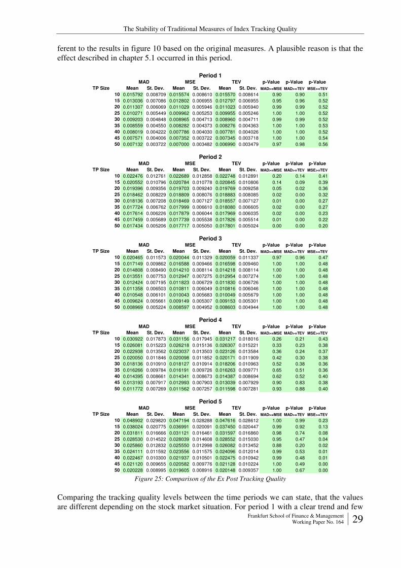
The Stability of Traditional Measures of Index Tracking Quality
Frankfurt School of Finance & Management Working Paper No. 164 29
ferent to the results in figure 10 based on the original measures. A plausible reason is that the effect described in chapter 5.1 occurred in this period.
p-Value p-Value p-Value
TP Size Mean St. Dev. Mean St. Dev. Mean St. Dev. MAD>=MSE MAD>=TEV MSE>=TEV
10 0.015792 0.008709 0.015574 0.008610 0.015570 0.008614 0.90 0.90 0.51
15 0.013036 0.007086 0.012802 0.006955 0.012797 0.006955 0.95 0.96 0.52
20 0.011307 0.006069 0.011029 0.005946 0.011023 0.005940 0.99 0.99 0.52
25 0.010271 0.005449 0.009962 0.005253 0.009955 0.005246 1.00 1.00 0.52
30 0.009203 0.004848 0.008965 0.004713 0.008960 0.004711 0.99 0.99 0.52
35 0.008559 0.004550 0.008282 0.004373 0.008276 0.004363 1.00 1.00 0.53
40 0.008019 0.004222 0.007786 0.004030 0.007781 0.004026 1.00 1.00 0.52
45 0.007571 0.004006 0.007352 0.003722 0.007345 0.003718 1.00 1.00 0.54
50 0.007132 0.003722 0.007000 0.003482 0.006990 0.003479 0.97 0.98 0.56
p-Value p-Value p-Value
TP Size Mean St. Dev. Mean St. Dev. Mean St. Dev. MAD>=MSE MAD>=TEV MSE>=TEV
10 0.022476 0.012761 0.022689 0.012858 0.022748 0.012891 0.20 0.14 0.41
15 0.020552 0.010796 0.020784 0.010778 0.020845 0.010806 0.14 0.09 0.39
20 0.019396 0.009356 0.019703 0.009240 0.019769 0.009258 0.05 0.02 0.36
25 0.018462 0.008229 0.018809 0.008076 0.018883 0.008085 0.02 0.00 0.32
30 0.018136 0.007208 0.018469 0.007127 0.018557 0.007127 0.01 0.00 0.27
35 0.017724 0.006762 0.017999 0.006610 0.018080 0.006605 0.02 0.00 0.27
40 0.017614 0.006226 0.017879 0.006044 0.017969 0.006035 0.02 0.00 0.23
45 0.017459 0.005689 0.017739 0.005538 0.017826 0.005514 0.01 0.00 0.22
50 0.017434 0.005206 0.017717 0.005050 0.017801 0.005024 0.00 0.00 0.20
p-Value p-Value p-Value
TP Size Mean St. Dev. Mean St. Dev. Mean St. Dev. MAD>=MSE MAD>=TEV MSE>=TEV
10 0.020465 0.011573 0.020044 0.011329 0.020059 0.011337 0.97 0.96 0.47
15 0.017149 0.009862 0.016588 0.009466 0.016598 0.009460 1.00 1.00 0.48
20 0.014808 0.008490 0.014210 0.008114 0.014218 0.008114 1.00 1.00 0.48
25 0.013551 0.007753 0.012947 0.007275 0.012954 0.007274 1.00 1.00 0.48
30 0.012424 0.007195 0.011823 0.006729 0.011830 0.006726 1.00 1.00 0.48
35 0.011358 0.006503 0.010811 0.006049 0.010816 0.006046 1.00 1.00 0.48
40 0.010548 0.006101 0.010043 0.005683 0.010049 0.005679 1.00 1.00 0.48
45 0.009624 0.005661 0.009149 0.005307 0.009153 0.005301 1.00 1.00 0.48
50 0.008969 0.005224 0.008597 0.004952 0.008603 0.004944 1.00 1.00 0.48
p-Value p-Value p-Value
TP Size Mean St. Dev. Mean St. Dev. Mean St. Dev. MAD>=MSE MAD>=TEV MSE>=TEV
10 0.030922 0.017873 0.031156 0.017945 0.031217 0.018016 0.26 0.21 0.43
15 0.026081 0.015223 0.026218 0.015136 0.026307 0.015221 0.33 0.23 0.38
20 0.022938 0.013562 0.023037 0.013503 0.023126 0.013584 0.36 0.24 0.37
25 0.020050 0.011846 0.020098 0.011852 0.020171 0.011909 0.42 0.30 0.38
30 0.018136 0.010910 0.018127 0.010914 0.018206 0.010963 0.52 0.38 0.36
35 0.016266 0.009784 0.016191 0.009726 0.016263 0.009771 0.65 0.51 0.36
40 0.014395 0.008661 0.014341 0.008673 0.014387 0.008694 0.62 0.52 0.40
45 0.013193 0.007917 0.012993 0.007903 0.013039 0.007929 0.90 0.83 0.38
50 0.011772 0.007269 0.011562 0.007257 0.011598 0.007281 0.93 0.88 0.40
p-Value p-Value p-Value
TP Size Mean St. Dev. Mean St. Dev. Mean St. Dev. MAD>=MSE MAD>=TEV MSE>=TEV
10 0.048902 0.029820 0.047194 0.028288 0.047616 0.028612 1.00 0.99 0.23
15 0.038024 0.020775 0.036991 0.020091 0.037450 0.020447 0.99 0.92 0.13
20 0.031811 0.016666 0.031121 0.016461 0.031597 0.016860 0.98 0.74 0.08
25 0.028530 0.014522 0.028039 0.014608 0.028552 0.015030 0.95 0.47 0.04
30 0.025860 0.012832 0.025550 0.012998 0.026082 0.013452 0.88 0.20 0.02
35 0.024111 0.011592 0.023556 0.011575 0.024096 0.012014 0.99 0.53 0.01
40 0.022467 0.010300 0.021937 0.010501 0.022475 0.010942 0.99 0.48 0.01
45 0.021120 0.009655 0.020582 0.009776 0.021128 0.010224 1.00 0.49 0.00
50 0.020228 0.008995 0.019605 0.008916 0.020148 0.009357 1.00 0.67 0.00
MAD MSE TEV
Period 1
Period 2
Period 3
Period 4
Period 5
MAD MSE TEV
MAD MSE TEV
MAD MSE TEV
MAD MSE TEV
Figure 25: Comparison of the Ex Post Tracking Quality
Comparing the tracking quality levels between the time periods we can state, that the values are different depending on the stock market situation. For period 1 with a clear trend and few
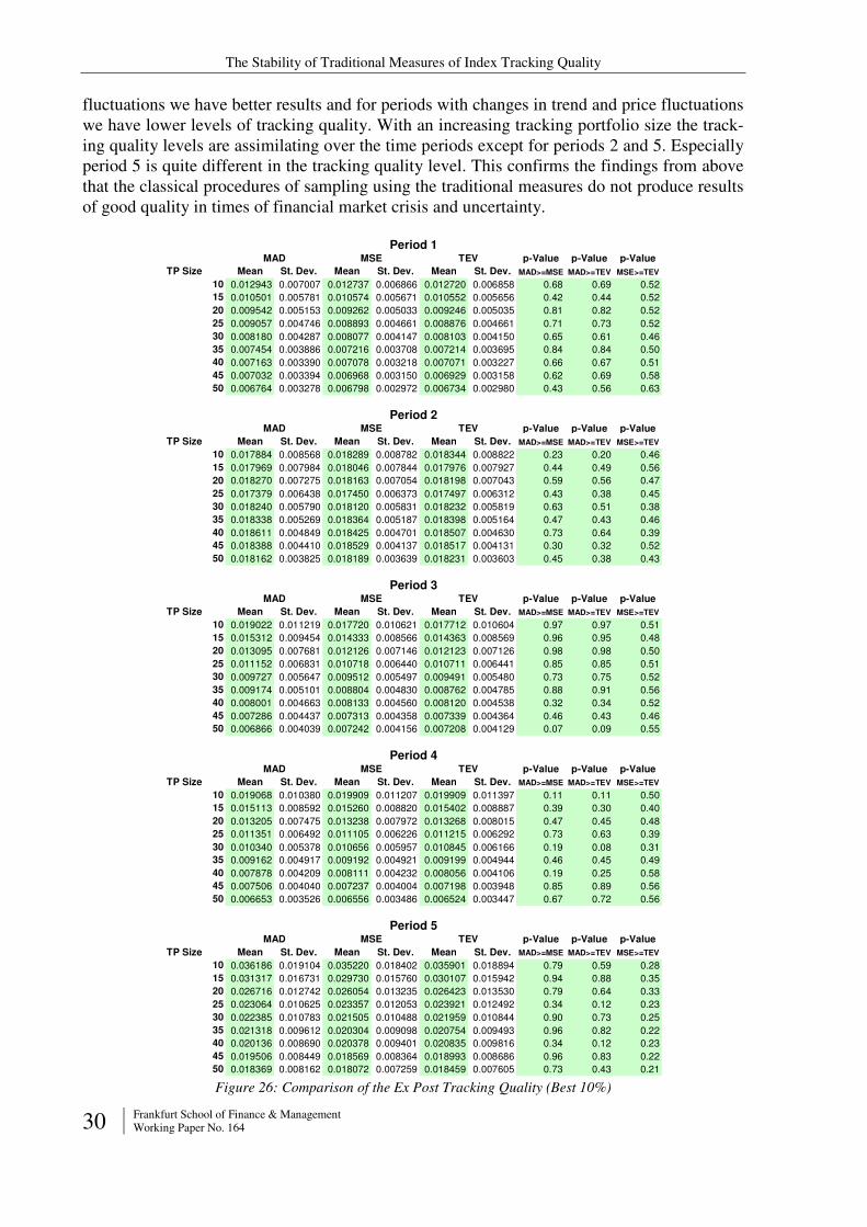
The Stability of Traditional Measures of Index Tracking Quality
30 Frankfurt School of Finance & Management Working Paper No. 164
fluctuations we have better results and for periods with changes in trend and price fluctuations we have lower levels of tracking quality. With an increasing tracking portfolio size the track-ing quality levels are assimilating over the time periods except for periods 2 and 5. Especially period 5 is quite different in the tracking quality level. This confirms the findings from above that the classical procedures of sampling using the traditional measures do not produce results of good quality in times of financial market crisis and uncertainty.
p-Value p-Value p-Value
TP Size Mean St. Dev. Mean St. Dev. Mean St. Dev. MAD>=MSE MAD>=TEV MSE>=TEV
10 0.012943 0.007007 0.012737 0.006866 0.012720 0.006858 0.68 0.69 0.52
15 0.010501 0.005781 0.010574 0.005671 0.010552 0.005656 0.42 0.44 0.52
20 0.009542 0.005153 0.009262 0.005033 0.009246 0.005035 0.81 0.82 0.52
25 0.009057 0.004746 0.008893 0.004661 0.008876 0.004661 0.71 0.73 0.52
30 0.008180 0.004287 0.008077 0.004147 0.008103 0.004150 0.65 0.61 0.46
35 0.007454 0.003886 0.007216 0.003708 0.007214 0.003695 0.84 0.84 0.50
40 0.007163 0.003390 0.007078 0.003218 0.007071 0.003227 0.66 0.67 0.51
45 0.007032 0.003394 0.006968 0.003150 0.006929 0.003158 0.62 0.69 0.58
50 0.006764 0.003278 0.006798 0.002972 0.006734 0.002980 0.43 0.56 0.63
p-Value p-Value p-Value
TP Size Mean St. Dev. Mean St. Dev. Mean St. Dev. MAD>=MSE MAD>=TEV MSE>=TEV
10 0.017884 0.008568 0.018289 0.008782 0.018344 0.008822 0.23 0.20 0.46
15 0.017969 0.007984 0.018046 0.007844 0.017976 0.007927 0.44 0.49 0.56
20 0.018270 0.007275 0.018163 0.007054 0.018198 0.007043 0.59 0.56 0.47
25 0.017379 0.006438 0.017450 0.006373 0.017497 0.006312 0.43 0.38 0.45
30 0.018240 0.005790 0.018120 0.005831 0.018232 0.005819 0.63 0.51 0.38
35 0.018338 0.005269 0.018364 0.005187 0.018398 0.005164 0.47 0.43 0.46
40 0.018611 0.004849 0.018425 0.004701 0.018507 0.004630 0.73 0.64 0.39
45 0.018388 0.004410 0.018529 0.004137 0.018517 0.004131 0.30 0.32 0.52
50 0.018162 0.003825 0.018189 0.003639 0.018231 0.003603 0.45 0.38 0.43
p-Value p-Value p-Value
TP Size Mean St. Dev. Mean St. Dev. Mean St. Dev. MAD>=MSE MAD>=TEV MSE>=TEV
10 0.019022 0.011219 0.017720 0.010621 0.017712 0.010604 0.97 0.97 0.51
15 0.015312 0.009454 0.014333 0.008566 0.014363 0.008569 0.96 0.95 0.48
20 0.013095 0.007681 0.012126 0.007146 0.012123 0.007126 0.98 0.98 0.50
25 0.011152 0.006831 0.010718 0.006440 0.010711 0.006441 0.85 0.85 0.51
30 0.009727 0.005647 0.009512 0.005497 0.009491 0.005480 0.73 0.75 0.52
35 0.009174 0.005101 0.008804 0.004830 0.008762 0.004785 0.88 0.91 0.56
40 0.008001 0.004663 0.008133 0.004560 0.008120 0.004538 0.32 0.34 0.52
45 0.007286 0.004437 0.007313 0.004358 0.007339 0.004364 0.46 0.43 0.46
50 0.006866 0.004039 0.007242 0.004156 0.007208 0.004129 0.07 0.09 0.55
p-Value p-Value p-Value
TP Size Mean St. Dev. Mean St. Dev. Mean St. Dev. MAD>=MSE MAD>=TEV MSE>=TEV
10 0.019068 0.010380 0.019909 0.011207 0.019909 0.011397 0.11 0.11 0.50
15 0.015113 0.008592 0.015260 0.008820 0.015402 0.008887 0.39 0.30 0.40
20 0.013205 0.007475 0.013238 0.007972 0.013268 0.008015 0.47 0.45 0.48
25 0.011351 0.006492 0.011105 0.006226 0.011215 0.006292 0.73 0.63 0.39
30 0.010340 0.005378 0.010656 0.005957 0.010845 0.006166 0.19 0.08 0.31
35 0.009162 0.004917 0.009192 0.004921 0.009199 0.004944 0.46 0.45 0.49
40 0.007878 0.004209 0.008111 0.004232 0.008056 0.004106 0.19 0.25 0.58
45 0.007506 0.004040 0.007237 0.004004 0.007198 0.003948 0.85 0.89 0.56
50 0.006653 0.003526 0.006556 0.003486 0.006524 0.003447 0.67 0.72 0.56
p-Value p-Value p-Value
TP Size Mean St. Dev. Mean St. Dev. Mean St. Dev. MAD>=MSE MAD>=TEV MSE>=TEV
10 0.036186 0.019104 0.035220 0.018402 0.035901 0.018894 0.79 0.59 0.28
15 0.031317 0.016731 0.029730 0.015760 0.030107 0.015942 0.94 0.88 0.35
20 0.026716 0.012742 0.026054 0.013235 0.026423 0.013530 0.79 0.64 0.33
25 0.023064 0.010625 0.023357 0.012053 0.023921 0.012492 0.34 0.12 0.23
30 0.022385 0.010783 0.021505 0.010488 0.021959 0.010844 0.90 0.73 0.25
35 0.021318 0.009612 0.020304 0.009098 0.020754 0.009493 0.96 0.82 0.22
40 0.020136 0.008690 0.020378 0.009401 0.020835 0.009816 0.34 0.12 0.23
45 0.019506 0.008449 0.018569 0.008364 0.018993 0.008686 0.96 0.83 0.22
50 0.018369 0.008162 0.018072 0.007259 0.018459 0.007605 0.73 0.43 0.21
MAD MSE TEV
MAD MSE TEV
Period 2
Period 3
Period 4
Period 5
MAD MSE TEV
MAD MSE TEV
MAD MSE TEV
Period 1
Figure 26: Comparison of the Ex Post Tracking Quality (Best 10%)
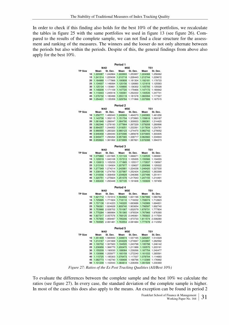
The Stability of Traditional Measures of Index Tracking Quality
Frankfurt School of Finance & Management Working Paper No. 164 31
In order to check if this finding also holds for the best 10% of the portfolios, we recalculate the tables in figure 25 with the same portfolios we used in figure 13 (see figure 26). Com-pared to the results of the complete sample, we can not find a clear structure for the assess-ment and ranking of the measures. The winners and the looser do not only alternate between the periods but also within the periods. Despite of this, the general findings from above also apply for the best 10%.
TP Size Mean St. Dev. Mean St. Dev. Mean St. Dev.
10 1.220087 1.242864 1.222693 1.253957 1.224068 1.256062
15 1.241314 1.225636 1.210718 1.226443 1.212744 1.229672
20 1.184968 1.177866 1.190808 1.181304 1.192181 1.179733
25 1.134007 1.148084 1.120156 1.126880 1.121619 1.125583
30 1.125134 1.130661 1.109890 1.136302 1.105793 1.135028
35 1.148208 1.171109 1.147720 1.179466 1.147172 1.180842
40 1.119443 1.245518 1.100091 1.252222 1.100535 1.247731
45 1.076732 1.180499 1.055119 1.181578 1.060094 1.177327
50 1.054431 1.135358 1.029784 1.171866 1.037999 1.167515
TP Size Mean St. Dev. Mean St. Dev. Mean St. Dev.
10 1.256777 1.489343 1.240604 1.464073 1.240083 1.461256
15 1.143736 1.352115 1.151704 1.373993 1.159616 1.363187
20 1.061648 1.286047 1.084790 1.309933 1.086361 1.314420
25 1.062346 1.278193 1.077864 1.267229 1.079208 1.280896
30 0.994257 1.244952 1.019251 1.222261 1.017834 1.224791
35 0.966555 1.283320 0.980123 1.274470 0.982742 1.279052
40 0.946458 1.284040 0.970396 1.285678 0.970905 1.303305
45 0.949477 1.290264 0.957365 1.338717 0.962660 1.334844
50 0.959924 1.361062 0.973999 1.387821 0.976398 1.394373
TP Size Mean St. Dev. Mean St. Dev. Mean St. Dev.
10 1.075860 1.031565 1.131124 1.066671 1.132535 1.069061
15 1.120019 1.043108 1.157313 1.105005 1.155566 1.104055
20 1.130813 1.105233 1.171865 1.135517 1.172837 1.138567
25 1.215193 1.134924 1.207977 1.129637 1.209366 1.129322
30 1.277349 1.274214 1.242981 1.224038 1.246420 1.227530
35 1.238106 1.274750 1.227987 1.252424 1.234522 1.263399
40 1.318356 1.308459 1.234829 1.246366 1.237496 1.251411
45 1.320751 1.275824 1.251078 1.217643 1.247155 1.214491
50 1.306430 1.293448 1.187105 1.191608 1.193609 1.197458
TP Size Mean St. Dev. Mean St. Dev. Mean St. Dev.
10 1.621712 1.721913 1.564962 1.601196 1.567986 1.580782
15 1.725695 1.771824 1.718110 1.716032 1.708074 1.712823
20 1.737138 1.814223 1.740220 1.693686 1.742989 1.694831
25 1.766361 1.824628 1.809740 1.903654 1.798597 1.892740
30 1.753968 2.028702 1.701067 1.832079 1.678731 1.777804
35 1.775284 1.989984 1.761360 1.976534 1.767966 1.976380
40 1.827317 2.057576 1.768125 2.049361 1.785922 2.117554
45 1.757655 1.959497 1.795206 1.973733 1.811574 2.008280
50 1.769585 2.061481 1.763554 2.081684 1.777678 2.112352
TP Size Mean St. Dev. Mean St. Dev. Mean St. Dev.
10 1.351409 1.560930 1.339974 1.537165 1.326297 1.514329
15 1.214167 1.241669 1.244229 1.274847 1.243887 1.282592
20 1.190702 1.307920 1.194505 1.243798 1.195798 1.246142
25 1.236958 1.366770 1.200470 1.211988 1.193570 1.203191
30 1.155209 1.190030 1.188084 1.239266 1.187754 1.240477
35 1.130998 1.205977 1.160159 1.272240 1.161033 1.265591
40 1.115725 1.185303 1.076473 1.117037 1.078704 1.114683
45 1.082773 1.142740 1.108408 1.168796 1.112389 1.176992
50 1.101239 1.102043 1.084814 1.228356 1.091509 1.230369
MAD MSE TEV
MAD MSE TEV
Period 2
Period 3
Period 4
Period 5
MAD MSE TEV
MAD MSE TEV
MAD MSE TEV
Period 1
Figure 27: Ratios of the Ex Post Tracking Qualities (All/Best 10%)
To evaluate the differences between the complete sample and the best 10% we calculate the ratios (see figure 27). In every case, the standard deviation of the complete sample is higher. In most of the cases this does also apply to the means. An exception can be found in period 2
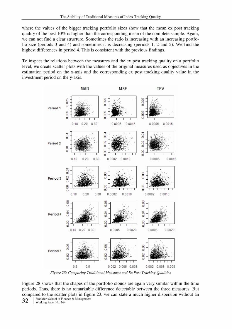
The Stability of Traditional Measures of Index Tracking Quality
32 Frankfurt School of Finance & Management Working Paper No. 164
where the values of the bigger tracking portfolio sizes show that the mean ex post tracking quality of the best 10% is higher than the corresponding mean of the complete sample. Again, we can not find a clear structure. Sometimes the ratio is increasing with an increasing portfo-lio size (periods 3 and 4) and sometimes it is decreasing (periods 1, 2 and 5). We find the highest differences in period 4. This is consistent with the previous findings.
To inspect the relations between the measures and the ex post tracking quality on a portfolio level, we create scatter plots with the values of the original measures used as objectives in the estimation period on the x-axis and the corresponding ex post tracking quality value in the investment period on the y-axis.
Figure 28: Comparing Traditional Measures and Ex Post Tracking Qualities
Figure 28 shows that the shapes of the portfolio clouds are again very similar within the time periods. Thus, there is no remarkable difference detectable between the three measures. But compared to the scatter plots in figure 23, we can state a much higher dispersion without an
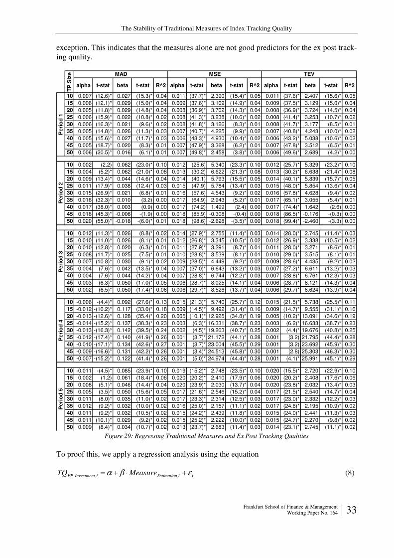
The Stability of Traditional Measures of Index Tracking Quality
Frankfurt School of Finance & Management Working Paper No. 164 33
exception. This indicates that the measures alone are not good predictors for the ex post track-ing quality.
alpha t-stat beta t-stat R^2 alpha t-stat beta t-stat R^2 alpha t-stat beta t-stat R^2
10 0.007 (12.6)* 0.027 (15.3)* 0.04 0.011 (37.7)* 2.390 (15.4)* 0.05 0.011 (37.6)* 2.407 (15.6)* 0.05
15 0.006 (12.1)* 0.029 (15.0)* 0.04 0.009 (37.6)* 3.109 (14.9)* 0.04 0.009 (37.5)* 3.129 (15.0)* 0.04
20 0.005 (11.8)* 0.029 (14.8)* 0.04 0.008 (36.9)* 3.702 (14.3)* 0.04 0.008 (36.9)* 3.724 (14.5)* 0.04
25 0.006 (15.9)* 0.022 (10.8)* 0.02 0.008 (41.3)* 3.238 (10.6)* 0.02 0.008 (41.4)* 3.253 (10.7)* 0.02
30 0.006 (16.3)* 0.021 (9.6)* 0.02 0.008 (41.8)* 3.126 (8.3)* 0.01 0.008 (41.7)* 3.177 (8.5)* 0.01
35 0.005 (14.8)* 0.026 (11.3)* 0.03 0.007 (40.7)* 4.225 (9.9)* 0.02 0.007 (40.8)* 4.243 (10.0)* 0.02
40 0.005 (15.6)* 0.027 (11.7)* 0.03 0.006 (43.3)* 4.930 (10.4)* 0.02 0.006 (43.2)* 5.038 (10.6)* 0.02
45 0.005 (18.7)* 0.020 (8.3)* 0.01 0.007 (47.9)* 3.368 (6.2)* 0.01 0.007 (47.8)* 3.512 (6.5)* 0.01
50 0.006 (20.5)* 0.016 (6.1)* 0.01 0.007 (49.8)* 2.458 (3.8)* 0.00 0.006 (49.6)* 2.689 (4.2)* 0.00
10 0.002 (2.2) 0.062 (23.0)* 0.10 0.012 (25.6) 5.340 (23.3)* 0.10 0.012 (25.7)* 5.329 (23.2)* 0.10
15 0.004 (5.2)* 0.062 (21.0)* 0.08 0.013 (30.2) 6.622 (21.3)* 0.08 0.013 (30.2)* 6.638 (21.4)* 0.08
20 0.009 (13.4)* 0.044 (14.6)* 0.04 0.014 (40.1) 5.793 (15.5)* 0.05 0.014 (40.1)* 5.839 (15.7)* 0.05
25 0.011 (17.9)* 0.038 (12.4)* 0.03 0.015 (47.9) 5.784 (13.4)* 0.03 0.015 (48.0)* 5.854 (13.6)* 0.04
30 0.015 (26.9)* 0.021 (6.8)* 0.01 0.016 (57.6) 4.543 (9.2)* 0.02 0.016 (57.8)* 4.628 (9.4)* 0.02
35 0.016 (32.3)* 0.010 (3.2) 0.00 0.017 (64.9) 2.943 (5.2)* 0.01 0.017 (65.1)* 3.055 (5.4)* 0.01
40 0.017 (38.0)* 0.003 (0.9) 0.00 0.017 (74.2) 1.499 (2.4) 0.00 0.017 (74.4)* 1.642 (2.6) 0.00
45 0.018 (45.3)* -0.006 -(1.9) 0.00 0.018 (85.9) -0.308 -(0.4) 0.00 0.018 (86.5)* -0.176 -(0.3) 0.00
50 0.020 (55.0)* -0.018 -(6.0)* 0.01 0.018 (98.6) -2.628 -(3.5)* 0.00 0.018 (99.4)* -2.460 -(3.3) 0.00
10 0.012 (11.3)* 0.026 (8.8)* 0.02 0.014 (27.9)* 2.755 (11.4)* 0.03 0.014 (28.0)* 2.745 (11.4)* 0.03
15 0.010 (11.0)* 0.026 (8.1)* 0.01 0.012 (26.8)* 3.345 (10.5)* 0.02 0.012 (26.9)* 3.338 (10.5)* 0.02
20 0.010 (12.8)* 0.020 (6.3)* 0.01 0.011 (27.9)* 3.291 (8.7)* 0.01 0.011 (28.0)* 3.271 (8.6)* 0.01
25 0.008 (11.7)* 0.025 (7.5)* 0.01 0.010 (28.8)* 3.539 (8.1)* 0.01 0.010 (29.0)* 3.515 (8.1)* 0.01
30 0.007 (10.8)* 0.030 (9.1)* 0.02 0.009 (28.5)* 4.449 (9.2)* 0.02 0.009 (28.6)* 4.435 (9.2)* 0.02
35 0.004 (7.6)* 0.042 (13.5)* 0.04 0.007 (27.0)* 6.643 (13.2)* 0.03 0.007 (27.2)* 6.611 (13.2)* 0.03
40 0.004 (7.6)* 0.044 (14.2)* 0.04 0.007 (28.8)* 6.744 (12.2)* 0.03 0.007 (28.8)* 6.761 (12.3)* 0.03
45 0.003 (6.3)* 0.050 (17.0)* 0.05 0.006 (28.7)* 8.025 (14.1)* 0.04 0.006 (28.7)* 8.121 (14.3)* 0.04
50 0.002 (6.5)* 0.050 (17.4)* 0.06 0.006 (29.7)* 8.526 (13.7)* 0.04 0.006 (29.7)* 8.624 (13.9)* 0.04
10 -0.006 -(4.4)* 0.092 (27.6)* 0.13 0.015 (21.3)* 5.740 (25.7)* 0.12 0.015 (21.5)* 5.738 (25.5)* 0.11
15 -0.012 -(10.2)* 0.117 (33.0)* 0.18 0.009 (14.5)* 9.492 (31.4)* 0.16 0.009 (14.7)* 9.555 (31.1)* 0.16
20 -0.013 -(12.6)* 0.128 (35.4)* 0.20 0.005 (10.1)* 12.925 (34.8)* 0.19 0.005 (10.2)* 13.091 (34.6)* 0.19
25 -0.014 -(15.2)* 0.137 (38.3)* 0.23 0.003 (6.3)* 16.331 (38.7)* 0.23 0.003 (6.2)* 16.633 (38.7)* 0.23
30 -0.013 -(16.3)* 0.142 (39.5)* 0.24 0.002 (4.5)* 19.263 (40.7)* 0.25 0.002 (4.4)* 19.676 (40.8)* 0.25
35 -0.012 -(17.4)* 0.140 (41.9)* 0.26 0.001 (3.7)* 21.172 (44.1)* 0.28 0.001 (3.2) 21.795 (44.4)* 0.28
40 -0.010 -(17.1)* 0.134 (42.6)* 0.27 0.001 (3.7)* 23.004 (45.5)* 0.29 0.001 (3.2) 23.692 (45.9)* 0.30
45 -0.009 -(16.6)* 0.131 (42.2)* 0.26 0.001 (3.4)* 24.513 (45.8)* 0.30 0.001 (2.8) 25.303 (46.3)* 0.30
50 -0.007 -(15.2)* 0.122 (41.4)* 0.26 0.001 (5.0)* 24.974 (44.4)* 0.28 0.001 (4.1)* 25.991 (45.1)* 0.29
10 -0.011 -(4.5)* 0.085 (23.9)* 0.10 0.019 (15.2)* 2.748 (23.5)* 0.10 0.020 (15.5)* 2.720 (22.9)* 0.10
15 0.002 (1.2) 0.061 (18.4)* 0.06 0.020 (20.2)* 2.410 (17.9)* 0.06 0.020 (20.2)* 2.408 (17.6)* 0.06
20 0.008 (5.1)* 0.046 (14.4)* 0.04 0.020 (23.9)* 2.030 (13.7)* 0.04 0.020 (23.8)* 2.032 (13.4)* 0.03
25 0.005 (3.5)* 0.050 (15.6)* 0.05 0.017 (21.6)* 2.546 (15.2)* 0.04 0.017 (21.5)* 2.540 (14.7)* 0.04
30 0.011 (8.0)* 0.035 (11.0)* 0.02 0.017 (23.3)* 2.314 (12.5)* 0.03 0.017 (23.0)* 2.332 (12.2)* 0.03
35 0.012 (9.2)* 0.032 (10.0)* 0.02 0.016 (25.0)* 2.157 (11.1)* 0.02 0.017 (24.6)* 2.195 (10.9)* 0.02
40 0.011 (9.2)* 0.032 (10.5)* 0.02 0.015 (24.2)* 2.439 (11.8)* 0.03 0.015 (24.0)* 2.441 (11.3)* 0.03
45 0.011 (10.1)* 0.029 (9.2)* 0.02 0.015 (25.2)* 2.222 (10.0)* 0.02 0.015 (24.7)* 2.270 (9.8)* 0.02
50 0.009 (8.4)* 0.034 (10.7)* 0.02 0.013 (23.7)* 2.683 (11.4)* 0.03 0.014 (23.1)* 2.745 (11.1)* 0.02
Peri
od
4P
eri
od
2P
eri
od
5
TP
Siz
e
Peri
od
3
MAD MSE TEV
Peri
od
1
Figure 29: Regressing Traditional Measures and Ex Post Tracking Qualities
To proof this, we apply a regression analysis using the equation
ii,Estimationi,Investment,EP MeasureTQ εβα +⋅+= (8)
The Stability of Traditional Measures of Index Tracking Quality
34 Frankfurt School of Finance & Management Working Paper No. 164
Here, the R2 is especially of interest because it expresses the quality of the measure as a pre-dictor for the ex post tracking quality. The results shown in Figure 29 confirm that the meas-ures alone are not good predictors for the ex post tracking quality. The majority of the R2 val-ues range below 5%. Only in period 4 we have about 20%. But even these values are very low.
The compounding of the deviations between the tracking portfolio and index from day to day can explain the poor tracking quality by the ex post tracking quality measure. For example, if there exists one large deviation at the beginning of the investment period, it rolls up in the next days and can significantly reduce the quality of tracking. This can be seen if we rewrite formula (6) in an equivalent form
∑ ∏∏= ==
+−+=T
t
t
i
iP
t
i
iI rrT
TQep1 1
,1
, )1()1(1
(9)
Fortunately, looking at the scatter plots, we can see that there exist tracking portfolios with high tracking qualities even in the estimation and the investment period. This raises the ques-tion, how they can be found.
6 Summary and Outlook
The purpose of this paper was to analyze the stability and performance of the traditional measures of tracking quality when used as objective in sampling. In the theoretical part in chapter 4, we first compared the concepts of the three measures MAD, MSE and TEV and elaborated some weaknesses when using them as a measure to evaluate the ex post tracking quality.
In the empirical part in chapter 5.3, we achieved several findings. One main finding is that the stock market phase has a sustainable influence on the tracking quality. The more there are turbulences like trend changes or strong price oscillations on the market the worse is the tracking quality when applying sampling via minimizing the specific measure. In these cases, the differences between the tracking quality calculated in the estimation period and the track-ing quality really achieved in the investment period are increasing. The greater this difference the less reliable is the tracking quality calculated in the estimation period as a predictor for the future tracking quality. Thus, the latter is underestimated due to an overfitting effect. This applies for all the three measures.
Another finding is that the differences in tracking quality between the different market phases decrease disproportional with increasing tracking portfolio sizes. This leads to the conclusion that the tracking portfolio size should be increased in turbulent markets to achieve a target tracking quality.
On the other hand, we find increasing differences in tracking quality between the estimation period and the investment period with an increasing tracking portfolio size. This indicates an increasing overfitting effect meaning that the tracking quality enhancement in the estimation period resulting from a greater portfolio size does not proportionally apply to the investment period.

The Stability of Traditional Measures of Index Tracking Quality
Frankfurt School of Finance & Management Working Paper No. 164 35
Our analyses show, that the traditional measures used in sampling not only have weaknesses in their absolute stability but also have a poor relative stability on average. Independent from the stock market phase, the relative tracking quality in the estimation period compared to al-ternative tracking portfolios is not a good predictor for the relative tracking quality in the in-vestment period. Thus, the tracking portfolio with the best tracking quality in the estimation period might not necessarily belong to the best ones in the investment period and vice versa. As a consequence, the commonly used sampling procedure of searching the tracking portfolio with the minimal value of the used tracking quality measure is not leading to the desired result independent of the measure used in the optimization process.
According to the definition of the ex post tracking quality, we used in this paper, all three measures show very poor results when used as a predictor for this ex post tracking quality. On average, there is just a marginal coherence. This raises the question if the traditional measures are really suitable for the sampling process.
The empirical results, which are also confirmed by another analysis with the S&P1500, also show that there exist tracking portfolios with high tracking qualities even in the estimation period and the investment period. This leads to several questions for further research. As stated before, one important question is, if an alternative measure can be found with a better ability for the prediction of the future tracking quality and therefore has a better ability against overfitting.
In addition, it seems worth to search for methods to calculate the tracking portfolios with a focus on robustness as an alternative to the commonly used optimization methods. A promis-ing approach with an alternative tracking quality measure based on Support Vector Regres-sion can be found in Karlow and Rossbach.23
Finally, there is some evidence that also the process of selecting the stocks has an important influence on the robustness of the tracking portfolio and therefore on the ex post tracking quality. The commonly used procedures which are searching for the one combination of stocks providing a minimal value of the used measure does not seem to be appropriate as the results indicate. Instead, there is a need for research about the specific properties of stocks being suitable for sampling and how they can be identified.
23 Karlow/Rossbach (2011).
The Stability of Traditional Measures of Index Tracking Quality
36 Frankfurt School of Finance & Management Working Paper No. 164
References
Alexander, C.; Dimitriu, A. (2004): A Comparison of Cointegration and Tracking Error Mod-els for Mutual Funds and Hedge Funds. ISMA Centre Discussion Papers in Finance, No. 4.
Bamberg, G.; Wagner, N. (2000): Equity index replication with standard and robust regres-sion estimators, in: OR Spectrum, 22 (4), pp. 525-543.
Beasley, J.E.; Meade, N.; Chang, T.J. (2003): An evolutionary heuristic for the index tracking problem, in: European Journal of Operational Research, 148 (3), pp. 621-643.
Blume, M.E.; Edelen, R.M. (2004): S&P 500 indexers, tracking error, and liquidity, in: The Journal of Portfolio Management, 30, pp. 37-47.
Bogle, J.C. (1992): Selecting equity mutual funds, in: The Journal of Portfolio Management, 18 (2), pp. 94-100.
Bonafede, J. K. (2003): The Wilshire 5000 Total Market Index: The Logistics Behind Manag-ing the U.S. Stock Market, in: Journal of Indexes, Third Quarter.
Canakgoz, N.A.; Beasley, J.E. (2009): Mixed-integer programming approaches for index tracking and enhanced indexation, in: European Journal of Operational Research, 196 (1), pp. 384-399.
Corielli, F.; Marcellino, M. (2006): Factor based index tracking in: Journal of Banking & Fi-nance, 30 (8), pp. 2215-2233.
Chen, H.; Noronha, G.; Singal, V. (2006) Index changes and losses to index fund investors, in: Financial Analysts Journal, 62 (4), pp. 31-47
Dose, C.; Cincotti, S. (2005): Clustering of financial time series with application to index and enhanced index tracking portfolio, in: Physica A: Statistical Mechanics and its Applica-tions, 355 (1), pp. 145-151
Focardi, S.M.; Fabozzi, F.J. (2004): A methodology for index tracking based on time-series clustering, in: Quantitative Finance, 4 (4), pp. 417-425.
French, K.R. (2008): Presidential address: The cost of active investing, in: The Journal of Finance, 63 (4), pp. 1537-1573.
Fuhr, D.; Kelly, S. (2010) ETF landscape industry review, August 2010, BlackRock.
Gaivoronski, A.A.; Krylov, S.; van der Wijst, N, (2005): Optimal portfolio selection and dy-namic benchmark tracking in: European journal of operational research, 163 (1), pp. 115-131.
Gilli, M.; Kellezi, M.G. (2001): Threshold Accepting for Index Tracking, Working Paper, Department of Econometrics, University of Geneva.
Hill, J.; Mueller, B. (2004): Choosing among Index Vehicles: How Does an Institutional In-vestor Select an Investment Product? in: Schoenfeld, S.A. (ed.): Active Index Investing, Wiley, New Jersey, pp. 503-534.
Hopkins, P.J.B.; Miller, C.H. (2001): Country, sector and company factors in global equity portfolios, The Research Foundation of AIMR, Charlottesville.
The Stability of Traditional Measures of Index Tracking Quality
Frankfurt School of Finance & Management Working Paper No. 164 37
Karlow, D.; Roßbach, P. (2011) A method for robust index tracking, To appear in: Hu, B.; Morasch, K.; Siegle, M.; Pickl, S. (eds.): Operations Research Proceedings 2010, Springer.
Maringer, D. (2008): Constrained index tracking under loss aversion using differential evolu-tion, in: Brabazon, A.; Neill, M. O. (eds.): Natural Computing in Computational Econom-ics and Finance, Springer, pp. 9-29.
Meade, N.; Salkin, G.R. (1989): Index funds-construction and performance measurement, in: Journal of the Operational Research Society, 40 (10), pp. 871-879.
Montfort, K.; Visser, E.; van Draat, L.F. (2008): Index tracking by means of optimized sam-pling, in: The Journal of Portfolio Management, 34 (2), pp. 143-152.
Roll, R. (1992) A mean/variance analysis of tracking error, in: The Journal of Portfolio Man-agement, 18 (4), pp. 13-22.
Roßbach, P.; Karlow, D. (2009): Index Tracking with Genetic Algorithms, Euro 2009, Bonn.
Rudd, A. (1980): Optimal selection of passive portfolios, in: Financial Management, 9 (1), pp. 57-66.
Rudolf, M.; Wolter, H.J.; Zimmermann, H (1999): A linear model for tracking error minimi-zation, in: Journal of Banking & Finance, 23 (1), pp. 85-103.
Rudolf, M (2009): Innovative Index Tracking Methoden, Vortragsfolien, Tagung: Finanz- und Vermögensberatung im Private Banking und Wealth Management, 10.06.2009, Frankfurt am Main.
Ruiz-Torrubiano, R.; Suarez, A. (2009): A hybrid optimization approach to index tracking, Springer.
Stoyan, S.J.; Kwon, R.H (2010): A two-stage stochastic mixed-integer programming ap-proach to the index tracking problem, in: Optimization and Engineering, 11 (2), pp. 247-275
Sharpe, W.F (1991): The arithmetic of active management, in: Financial Analysts Journal, 47 (1), pp. 7-9.
Schioldager, A.; Hahn, W.; Hoyt, E.; Leung, J (2004): The Unique Challenges of U.S. Equity Index Management, in: Schoenfeld, S.A. (ed.): Active Index Investing, Wiley, New Jer-sey, pp. 389-404.
The Stability of Traditional Measures of Index Tracking Quality
38 Frankfurt School of Finance & Management Working Paper No. 164
FRANKFURT SCHOOL / HFB – WORKING PAPER SERIES
No. Author/Title Year
163. Libman, Alexander / Herrmann-Pillath, Carsten / Yarav, Gaudav Are Human Rights and Economic Well-Being Substitutes? Evidence from Migration Patterns across the Indian States
2011
162. Herrmann-Pillath, Carsten / Andriani, Pierpaolo Transactional Innovation and the De-commoditization of the Brazilian Coffee Trade
2011
161. Christian Büchler, Marius Buxkaemper, Christoph Schalast, Gregor Wedell Incentivierung des Managements bei Unternehmenskäufen/Buy-Outs mit Private Equity Investoren – eine empirische Untersuchung –
2011
160. Herrmann-Pillath, Carsten Revisiting the Gaia Hypothesis: Maximum Entropy, Kauffman´s “Fourth Law” and Physiosemeiosis
2011
159. Herrmann-Pillath, Carsten A ‘Third Culture’ in Economics? An Essay on Smith, Confucius and the Rise of China
2011
158. Boeing. Philipp / Sandner, Philipp The Innovative Performance of China’s National Innovation System
2011
157. Herrmann-Pillath, Carsten Institutions, Distributed Cognition and Agency: Rule-following as Performative Action
2011
156. Wagner, Charlotte From Boom to Bust: How different has microfinance been from traditional banking?
2010
155. Libman Alexander / Vinokurov, Evgeny Is it really different? Patterns of Regionalisation in the Post-Soviet Central Asia
2010
154. Libman, Alexander Subnational Resource Curse: Do Economic or Political Institutions Matter?
2010
153. Herrmann-Pillath, Carsten Meaning and Function in the Theory of Consumer Choice: Dual Selves in Evolving Networks
2010
152. Kostka, Genia / Hobbs, William Embedded Interests and the Managerial Local State: Methanol Fuel-Switching in China
2010
151. Kostka, Genia / Hobbs, William Energy Efficiency in China: The Local Bundling of Interests and Policies
2010
150. Umber, Marc P. / Grote, Michael H. / Frey, Rainer Europe Integrates Less Than You Think. Evidence from the Market for Corporate Control in Europe and the US
2010
149. Vogel, Ursula / Winkler, Adalbert Foreign banks and financial stability in emerging markets: evidence from the global financial crisis
2010
148. Libman, Alexander Words or Deeds – What Matters? Experience of Decentralization in Russian Security Agencies
2010
147. Kostka, Genia / Zhou, Jianghua Chinese firms entering China's low-income market: Gaining competitive advantage by partnering governments
2010
146. Herrmann-Pillath, Carsten Rethinking Evolution, Entropy and Economics: A triadic conceptual framework for the Maximum Entropy Principle as applied to the growth of knowledge
2010
145. Heidorn, Thomas / Kahlert, Dennis Implied Correlations of iTraxx Tranches during the Financial Crisis
2010
144 Fritz-Morgenthal, Sebastian G. / Hach, Sebastian T. / Schalast, Christoph M&A im Bereich Erneuerbarer Energien
2010
143. Birkmeyer, Jörg / Heidorn, Thomas / Rogalski, André Determinanten von Banken-Spreads während der Finanzmarktkrise
2010
142. Bannier, Christina E. / Metz, Sabrina Are SMEs large firms en miniature? Evidence from a growth analysis
2010
141. Heidorn, Thomas / Kaiser, Dieter G. / Voinea, André The Value-Added of Investable Hedge Fund Indices
2010
140. Herrmann-Pillath, Carsten The Evolutionary Approach to Entropy: Reconciling Georgescu-Roegen’s Natural Philosophy with the Maximum Entropy Framework
2010
139. Heidorn, Thomas / Löw, Christian / Winker, Michael Funktionsweise und Replikationstil europäischer Exchange Traded Funds auf Aktienindices
2010
138. Libman, Alexander Constitutions, Regulations, and Taxes: Contradictions of Different Aspects of Decentralization
2010
The Stability of Traditional Measures of Index Tracking Quality
Frankfurt School of Finance & Management Working Paper No. 164 39
137. Herrmann-Pillath, Carsten / Libman, Alexander / Yu, Xiaofan State and market integration in China: A spatial econometrics approach to ‘local protectionism’
2010
136. Lang, Michael / Cremers, Heinz / Hentze, Rainald Ratingmodell zur Quantifizierung des Ausfallrisikos von LBO-Finanzierungen
2010
135. Bannier, Christina / Feess, Eberhard When high-powered incentive contracts reduce performance: Choking under pressure as a screening device
2010
134. Herrmann-Pillath, Carsten Entropy, Function and Evolution: Naturalizing Peircian Semiosis
2010
133. Bannier, Christina E. / Behr, Patrick / Güttler, Andre Rating opaque borrowers: why are unsolicited ratings lower?
2009
132. Herrmann-Pillath, Carsten Social Capital, Chinese Style: Individualism, Relational Collectivism and the Cultural Embeddedness of the Institu-tions-Performance Link
2009
131. Schäffler, Christian / Schmaltz, Christian Market Liquidity: An Introduction for Practitioners
2009
130. Herrmann-Pillath, Carsten Dimensionen des Wissens: Ein kognitiv-evolutionärer Ansatz auf der Grundlage von F.A. von Hayeks Theorie der „Sensory Order“
2009
129. Hankir, Yassin / Rauch, Christian / Umber, Marc It’s the Market Power, Stupid! – Stock Return Patterns in International Bank M&A
2009
128. Herrmann-Pillath, Carsten Outline of a Darwinian Theory of Money
2009
127. Cremers, Heinz / Walzner, Jens Modellierung des Kreditrisikos im Portfoliofall
2009
126. Cremers, Heinz / Walzner, Jens Modellierung des Kreditrisikos im Einwertpapierfall
2009
125. Heidorn, Thomas / Schmaltz, Christian Interne Transferpreise für Liquidität
2009
124. Bannier, Christina E. / Hirsch, Christian The economic function of credit rating agencies - What does the watchlist tell us?
2009
123. Herrmann-Pillath, Carsten A Neurolinguistic Approach to Performativity in Economics
2009
122. Winkler, Adalbert / Vogel, Ursula Finanzierungsstrukturen und makroökonomische Stabilität in den Ländern Südosteuropas, der Türkei und in den GUS-Staaten
2009
121. Heidorn, Thomas / Rupprecht, Stephan Einführung in das Kapitalstrukturmanagement bei Banken
2009
120. Rossbach, Peter Die Rolle des Internets als Informationsbeschaffungsmedium in Banken
2009
119. Herrmann-Pillath, Carsten Diversity Management und diversi-tätsbasiertes Controlling: Von der „Diversity Scorecard“ zur „Open Balanced Scorecard
2009
118. Hölscher, Luise / Clasen, Sven Erfolgsfaktoren von Private Equity Fonds
2009
117. Bannier, Christina E. Is there a hold-up benefit in heterogeneous multiple bank financing?
2009
116. Roßbach, Peter / Gießamer, Dirk Ein eLearning-System zur Unterstützung der Wissensvermittlung von Web-Entwicklern in Sicherheitsthemen
2009
115. Herrmann-Pillath, Carsten Kulturelle Hybridisierung und Wirtschaftstransformation in China
2009
114. Schalast, Christoph: Staatsfonds – „neue“ Akteure an den Finanzmärkten?
2009
113. Schalast, Christoph / Alram, Johannes Konstruktion einer Anleihe mit hypothekarischer Besicherung
2009
112. Schalast, Christoph / Bolder, Markus / Radünz, Claus / Siepmann, Stephanie / Weber, Thorsten Transaktionen und Servicing in der Finanzkrise: Berichte und Referate des Frankfurt School NPL Forums 2008
2009
111. Werner, Karl / Moormann, Jürgen Efficiency and Profitability of European Banks – How Important Is Operational Efficiency?
2009
The Stability of Traditional Measures of Index Tracking Quality
40 Frankfurt School of Finance & Management Working Paper No. 164
110. Herrmann-Pillath, Carsten Moralische Gefühle als Grundlage einer wohlstandschaffenden Wettbewerbsordnung: Ein neuer Ansatz zur erforschung von Sozialkapital und seine Anwendung auf China
2009
109. Heidorn, Thomas / Kaiser, Dieter G. / Roder, Christoph Empirische Analyse der Drawdowns von Dach-Hedgefonds
2009
108. Herrmann-Pillath, Carsten Neuroeconomics, Naturalism and Language
2008
107. Schalast, Christoph / Benita, Barten Private Equity und Familienunternehmen – eine Untersuchung unter besonderer Berücksichtigung deutscher Maschinen- und Anlagenbauunternehmen
2008
106. Bannier, Christina E. / Grote, Michael H. Equity Gap? – Which Equity Gap? On the Financing Structure of Germany’s Mittelstand
2008
105. Herrmann-Pillath, Carsten The Naturalistic Turn in Economics: Implications for the Theory of Finance
2008
104. Schalast, Christoph (Hrgs.) / Schanz, Kay-Michael / Scholl, Wolfgang Aktionärsschutz in der AG falsch verstanden? Die Leica-Entscheidung des LG Frankfurt am Main
2008
103. Bannier, Christina E./ Müsch, Stefan Die Auswirkungen der Subprime-Krise auf den deutschen LBO-Markt für Small- und MidCaps
2008
102. Cremers, Heinz / Vetter, Michael Das IRB-Modell des Kreditrisikos im Vergleich zum Modell einer logarithmisch normalverteilten Verlustfunktion
2008
101. Heidorn, Thomas / Pleißner, Mathias Determinanten Europäischer CMBS Spreads. Ein empirisches Modell zur Bestimmung der Risikoaufschläge von Commercial Mortgage-Backed Securities (CMBS)
2008
100. Schalast, Christoph (Hrsg.) / Schanz, Kay-Michael Schaeffler KG/Continental AG im Lichte der CSX Corp.-Entscheidung des US District Court for the Southern District of New York
2008
99. Hölscher, Luise / Haug, Michael / Schweinberger, Andreas Analyse von Steueramnestiedaten
2008
98. Heimer, Thomas / Arend, Sebastian The Genesis of the Black-Scholes Option Pricing Formula
2008
97. Heimer, Thomas / Hölscher, Luise / Werner, Matthias Ralf Access to Finance and Venture Capital for Industrial SMEs
2008
96. Böttger, Marc / Guthoff, Anja / Heidorn, Thomas Loss Given Default Modelle zur Schätzung von Recovery Rates
2008
95. Almer, Thomas / Heidorn, Thomas / Schmaltz, Christian The Dynamics of Short- and Long-Term CDS-spreads of Banks
2008
94. Barthel, Erich / Wollersheim, Jutta Kulturunterschiede bei Mergers & Acquisitions: Entwicklung eines Konzeptes zur Durchführung einer Cultural Due Diligence
2008
93. Heidorn, Thomas / Kunze, Wolfgang / Schmaltz, Christian Liquiditätsmodellierung von Kreditzusagen (Term Facilities and Revolver)
2008
92. Burger, Andreas Produktivität und Effizienz in Banken – Terminologie, Methoden und Status quo
2008
91. Löchel, Horst / Pecher, Florian The Strategic Value of Investments in Chinese Banks by Foreign Financial Insitutions
2008
90. Schalast, Christoph / Morgenschweis, Bernd / Sprengetter, Hans Otto / Ockens, Klaas / Stachuletz, Rainer / Safran, Robert Der deutsche NPL Markt 2007: Aktuelle Entwicklungen, Verkauf und Bewertung – Berichte und Referate des NPL Forums 2007
2008
89. Schalast, Christoph / Stralkowski, Ingo 10 Jahre deutsche Buyouts
2008
88. Bannier, Christina E./ Hirsch, Christian The Economics of Rating Watchlists: Evidence from Rating Changes
2007
87. Demidova-Menzel, Nadeshda / Heidorn, Thomas Gold in the Investment Portfolio
2007
86. Hölscher, Luise / Rosenthal, Johannes Leistungsmessung der Internen Revision
2007
85. Bannier, Christina / Hänsel, Dennis Determinants of banks' engagement in loan securitization
2007
The Stability of Traditional Measures of Index Tracking Quality
Frankfurt School of Finance & Management Working Paper No. 164 41
84. Bannier, Christina “Smoothing“ versus “Timeliness“ - Wann sind stabile Ratings optimal und welche Anforderungen sind an optimale Berichtsregeln zu stellen?
2007
83. Bannier, Christina E. Heterogeneous Multiple Bank Financing: Does it Reduce Inefficient Credit-Renegotiation Incidences?
2007
82. Cremers, Heinz / Löhr, Andreas Deskription und Bewertung strukturierter Produkte unter besonderer Berücksichtigung verschiedener Marktszenarien
2007
81. Demidova-Menzel, Nadeshda / Heidorn, Thomas Commodities in Asset Management
2007
80. Cremers, Heinz / Walzner, Jens Risikosteuerung mit Kreditderivaten unter besonderer Berücksichtigung von Credit Default Swaps
2007
79. Cremers, Heinz / Traughber, Patrick Handlungsalternativen einer Genossenschaftsbank im Investmentprozess unter Berücksichtigung der Risikotragfähig-keit
2007
78. Gerdesmeier, Dieter / Roffia, Barbara Monetary Analysis: A VAR Perspective
2007
77. Heidorn, Thomas / Kaiser, Dieter G. / Muschiol, Andrea Portfoliooptimierung mit Hedgefonds unter Berücksichtigung höherer Momente der Verteilung
2007
76. Jobe, Clemens J. / Ockens, Klaas / Safran, Robert / Schalast, Christoph Work-Out und Servicing von notleidenden Krediten – Berichte und Referate des HfB-NPL Servicing Forums 2006
2006
75. Abrar, Kamyar / Schalast, Christoph Fusionskontrolle in dynamischen Netzsektoren am Beispiel des Breitbandkabelsektors
2006
74. Schalast, Christoph / Schanz, Kay-Michael Wertpapierprospekte: Markteinführungspublizität nach EU-Prospektverordnung und Wertpapierprospektgesetz 2005
2006
73. Dickler, Robert A. / Schalast, Christoph Distressed Debt in Germany: What´s Next? Possible Innovative Exit Strategies
2006
72. Belke, Ansgar / Polleit, Thorsten How the ECB and the US Fed set interest rates
2006
71. Heidorn, Thomas / Hoppe, Christian / Kaiser, Dieter G. Heterogenität von Hedgefondsindizes
2006
70. Baumann, Stefan / Löchel, Horst The Endogeneity Approach of the Theory of Optimum Currency Areas - What does it mean for ASEAN + 3?
2006
69. Heidorn, Thomas / Trautmann, Alexandra Niederschlagsderivate
2005
68. Heidorn, Thomas / Hoppe, Christian / Kaiser, Dieter G. Möglichkeiten der Strukturierung von Hedgefondsportfolios
2005
67. Belke, Ansgar / Polleit, Thorsten (How) Do Stock Market Returns React to Monetary Policy ? An ARDL Cointegration Analysis for Germany
2005
66. Daynes, Christian / Schalast, Christoph Aktuelle Rechtsfragen des Bank- und Kapitalmarktsrechts II: Distressed Debt - Investing in Deutschland
2005
65. Gerdesmeier, Dieter / Polleit, Thorsten Measures of excess liquidity
2005
64. Becker, Gernot M. / Harding, Perham / Hölscher, Luise Financing the Embedded Value of Life Insurance Portfolios
2005
63. Schalast, Christoph Modernisierung der Wasserwirtschaft im Spannungsfeld von Umweltschutz und Wettbewerb – Braucht Deutschland eine Rechtsgrundlage für die Vergabe von Wasserversorgungskonzessionen? –
2005
62. Bayer, Marcus / Cremers, Heinz / Kluß, Norbert Wertsicherungsstrategien für das Asset Management
2005
61. Löchel, Horst / Polleit, Thorsten A case for money in the ECB monetary policy strategy
2005
60. Richard, Jörg / Schalast, Christoph / Schanz, Kay-Michael Unternehmen im Prime Standard - „Staying Public“ oder „Going Private“? - Nutzenanalyse der Börsennotiz -
2004
59. Heun, Michael / Schlink, Torsten Early Warning Systems of Financial Crises - Implementation of a currency crisis model for Uganda
2004
58. Heimer, Thomas / Köhler, Thomas Auswirkungen des Basel II Akkords auf österreichische KMU
2004
57. Heidorn, Thomas / Meyer, Bernd / Pietrowiak, Alexander Performanceeffekte nach Directors´Dealings in Deutschland, Italien und den Niederlanden
2004
The Stability of Traditional Measures of Index Tracking Quality
42 Frankfurt School of Finance & Management Working Paper No. 164
56. Gerdesmeier, Dieter / Roffia, Barbara The Relevance of real-time data in estimating reaction functions for the euro area
2004
55. Barthel, Erich / Gierig, Rauno / Kühn, Ilmhart-Wolfram Unterschiedliche Ansätze zur Messung des Humankapitals
2004
54. Anders, Dietmar / Binder, Andreas / Hesdahl, Ralf / Schalast, Christoph / Thöne, Thomas Aktuelle Rechtsfragen des Bank- und Kapitalmarktrechts I : Non-Performing-Loans / Faule Kredite - Handel, Work-Out, Outsourcing und Securitisation
2004
53. Polleit, Thorsten The Slowdown in German Bank Lending – Revisited
2004
52. Heidorn, Thomas / Siragusano, Tindaro Die Anwendbarkeit der Behavioral Finance im Devisenmarkt
2004
51. Schütze, Daniel / Schalast, Christoph (Hrsg.) Wider die Verschleuderung von Unternehmen durch Pfandversteigerung
2004
50. Gerhold, Mirko / Heidorn, Thomas Investitionen und Emissionen von Convertible Bonds (Wandelanleihen)
2004
49. Chevalier, Pierre / Heidorn, Thomas / Krieger, Christian Temperaturderivate zur strategischen Absicherung von Beschaffungs- und Absatzrisiken
2003
48. Becker, Gernot M. / Seeger, Norbert Internationale Cash Flow-Rechnungen aus Eigner- und Gläubigersicht
2003
47. Boenkost, Wolfram / Schmidt, Wolfgang M. Notes on convexity and quanto adjustments for interest rates and related options
2003
46. Hess, Dieter Determinants of the relative price impact of unanticipated Information in U.S. macroeconomic releases
2003
45. Cremers, Heinz / Kluß, Norbert / König, Markus Incentive Fees. Erfolgsabhängige Vergütungsmodelle deutscher Publikumsfonds
2003
44. Heidorn, Thomas / König, Lars Investitionen in Collateralized Debt Obligations
2003
43. Kahlert, Holger / Seeger, Norbert Bilanzierung von Unternehmenszusammenschlüssen nach US-GAAP
2003
42. Beiträge von Studierenden des Studiengangs BBA 012 unter Begleitung von Prof. Dr. Norbert Seeger Rechnungslegung im Umbruch - HGB-Bilanzierung im Wettbewerb mit den internationalen Standards nach IAS und US-GAAP
2003
41. Overbeck, Ludger / Schmidt, Wolfgang Modeling Default Dependence with Threshold Models
2003
40. Balthasar, Daniel / Cremers, Heinz / Schmidt, Michael Portfoliooptimierung mit Hedge Fonds unter besonderer Berücksichtigung der Risikokomponente
2002
39. Heidorn, Thomas / Kantwill, Jens Eine empirische Analyse der Spreadunterschiede von Festsatzanleihen zu Floatern im Euroraum und deren Zusammenhang zum Preis eines Credit Default Swaps
2002
38. Böttcher, Henner / Seeger, Norbert Bilanzierung von Finanzderivaten nach HGB, EstG, IAS und US-GAAP
2003
37. Moormann, Jürgen Terminologie und Glossar der Bankinformatik
2002
36. Heidorn, Thomas Bewertung von Kreditprodukten und Credit Default Swaps
2001
35. Heidorn, Thomas / Weier, Sven Einführung in die fundamentale Aktienanalyse
2001
34. Seeger, Norbert International Accounting Standards (IAS)
2001
33. Moormann, Jürgen / Stehling, Frank Strategic Positioning of E-Commerce Business Models in the Portfolio of Corporate Banking
2001
32. Sokolovsky, Zbynek / Strohhecker, Jürgen Fit für den Euro, Simulationsbasierte Euro-Maßnahmenplanung für Dresdner-Bank-Geschäftsstellen
2001
31. Roßbach, Peter Behavioral Finance - Eine Alternative zur vorherrschenden Kapitalmarkttheorie?
2001
30. Heidorn, Thomas / Jaster, Oliver / Willeitner, Ulrich Event Risk Covenants
2001
29. Biswas, Rita / Löchel, Horst Recent Trends in U.S. and German Banking: Convergence or Divergence?
2001
The Stability of Traditional Measures of Index Tracking Quality
Frankfurt School of Finance & Management Working Paper No. 164 43
28. Eberle, Günter Georg / Löchel, Horst Die Auswirkungen des Übergangs zum Kapitaldeckungsverfahren in der Rentenversicherung auf die Kapitalmärkte
2001
27. Heidorn, Thomas / Klein, Hans-Dieter / Siebrecht, Frank Economic Value Added zur Prognose der Performance europäischer Aktien
2000
26. Cremers, Heinz Konvergenz der binomialen Optionspreismodelle gegen das Modell von Black/Scholes/Merton
2000
25. Löchel, Horst Die ökonomischen Dimensionen der ‚New Economy‘
2000
24. Frank, Axel / Moormann, Jürgen Grenzen des Outsourcing: Eine Exploration am Beispiel von Direktbanken
2000
23. Heidorn, Thomas / Schmidt, Peter / Seiler, Stefan Neue Möglichkeiten durch die Namensaktie
2000
22. Böger, Andreas / Heidorn, Thomas / Graf Waldstein, Philipp Hybrides Kernkapital für Kreditinstitute
2000
21. Heidorn, Thomas Entscheidungsorientierte Mindestmargenkalkulation
2000
20. Wolf, Birgit Die Eigenmittelkonzeption des § 10 KWG
2000
19. Cremers, Heinz / Robé, Sophie / Thiele, Dirk Beta als Risikomaß - Eine Untersuchung am europäischen Aktienmarkt
2000
18. Cremers, Heinz Optionspreisbestimmung
1999
17. Cremers, Heinz Value at Risk-Konzepte für Marktrisiken
1999
16. Chevalier, Pierre / Heidorn, Thomas / Rütze, Merle Gründung einer deutschen Strombörse für Elektrizitätsderivate
1999
15. Deister, Daniel / Ehrlicher, Sven / Heidorn, Thomas CatBonds
1999
14. Jochum, Eduard Hoshin Kanri / Management by Policy (MbP)
1999
13. Heidorn, Thomas Kreditderivate
1999
12. Heidorn, Thomas Kreditrisiko (CreditMetrics)
1999
11. Moormann, Jürgen Terminologie und Glossar der Bankinformatik
1999
10. Löchel, Horst The EMU and the Theory of Optimum Currency Areas
1998
09. Löchel, Horst Die Geldpolitik im Währungsraum des Euro
1998
08. Heidorn, Thomas / Hund, Jürgen Die Umstellung auf die Stückaktie für deutsche Aktiengesellschaften
1998
07. Moormann, Jürgen Stand und Perspektiven der Informationsverarbeitung in Banken
1998
06. Heidorn, Thomas / Schmidt, Wolfgang LIBOR in Arrears
1998
05. Jahresbericht 1997 1998
04. Ecker, Thomas / Moormann, Jürgen Die Bank als Betreiberin einer elektronischen Shopping-Mall
1997
03. Jahresbericht 1996 1997
02. Cremers, Heinz / Schwarz, Willi Interpolation of Discount Factors
1996
01. Moormann, Jürgen Lean Reporting und Führungsinformationssysteme bei deutschen Finanzdienstleistern
1995

The Stability of Traditional Measures of Index Tracking Quality
44 Frankfurt School of Finance & Management Working Paper No. 164
FRANKFURT SCHOOL / HFB – WORKING PAPER SERIES
CENTRE FOR PRACTICAL QUANTITATIVE FINANCE
No. Author/Title Year
27. Detering, Nils / Weber, Andreas / Wystup, Uwe Return distributions of equity-linked retirement plans
2010
26. Veiga, Carlos / Wystup, Uwe Ratings of Structured Products and Issuers’ Commitments
2010
25. Beyna, Ingo / Wystup, Uwe On the Calibration of the Cheyette. Interest Rate Model
2010
24. Scholz, Peter / Walther, Ursula Investment Certificates under German Taxation. Benefit or Burden for Structured Products’ Performance
2010
23. Esquível, Manuel L. / Veiga, Carlos / Wystup, Uwe Unifying Exotic Option Closed Formulas
2010
22. Packham, Natalie / Schlögl, Lutz / Schmidt, Wolfgang M. Credit gap risk in a first passage time model with jumps
2009
21. Packham, Natalie / Schlögl, Lutz / Schmidt, Wolfgang M. Credit dynamics in a first passage time model with jumps
2009
20. Reiswich, Dimitri / Wystup, Uwe FX Volatility Smile Construction
2009
19. Reiswich, Dimitri / Tompkins, Robert Potential PCA Interpretation Problems for Volatility Smile Dynamics
2009
18. Keller-Ressel, Martin / Kilin, Fiodar Forward-Start Options in the Barndorff-Nielsen-Shephard Model
2008
17. Griebsch, Susanne / Wystup, Uwe On the Valuation of Fader and Discrete Barrier Options in Heston’s Stochastic Volatility Model
2008
16. Veiga, Carlos / Wystup, Uwe Closed Formula for Options with Discrete Dividends and its Derivatives
2008
15. Packham, Natalie / Schmidt, Wolfgang Latin hypercube sampling with dependence and applications in finance
2008
14. Hakala, Jürgen / Wystup, Uwe FX Basket Options
2008
13. Weber, Andreas / Wystup, Uwe Vergleich von Anlagestrategien bei Riesterrenten ohne Berücksichtigung von Gebühren. Eine Simulationsstudie zur Verteilung der Renditen
2008
12. Weber, Andreas / Wystup, Uwe Riesterrente im Vergleich. Eine Simulationsstudie zur Verteilung der Renditen
2008
11. Wystup, Uwe Vanna-Volga Pricing
2008
10. Wystup, Uwe Foreign Exchange Quanto Options
2008
09. Wystup, Uwe Foreign Exchange Symmetries
2008
08. Becker, Christoph / Wystup, Uwe Was kostet eine Garantie? Ein statistischer Vergleich der Rendite von langfristigen Anlagen
2008
07. Schmidt, Wolfgang Default Swaps and Hedging Credit Baskets
2007
06. Kilin, Fiodar Accelerating the Calibration of Stochastic Volatility Models
2007
05. Griebsch, Susanne/ Kühn, Christoph / Wystup, Uwe Instalment Options: A Closed-Form Solution and the Limiting Case
2007
04. Boenkost, Wolfram / Schmidt, Wolfgang M. Interest Rate Convexity and the Volatility Smile
2006
03. Becker, Christoph/ Wystup, Uwe On the Cost of Delayed Currency Fixing Announcements
2005
02. Boenkost, Wolfram / Schmidt, Wolfgang M. Cross currency swap valuation
2004

The Stability of Traditional Measures of Index Tracking Quality
Frankfurt School of Finance & Management Working Paper No. 164 45
01. Wallner, Christian / Wystup, Uwe Efficient Computation of Option Price Sensitivities for Options of American Style
2004
HFB – SONDERARBEITSBERICHTE DER HFB - BUSINESS SCHOOL OF FINANCE & MANAGEMENT
No. Author/Title Year
01. Nicole Kahmer / Jürgen Moormann Studie zur Ausrichtung von Banken an Kundenprozessen am Beispiel des Internet (Preis: € 120,--)
2003
Printed edition: € 25.00 + € 2.50 shipping
Download:
Working Paper: http://www.frankfurt-
school.de/content/de/research/publications/list_of_publication/list_of_publication
CPQF: http://www.frankfurt-school.de/content/de/cpqf/research_publications.html
Order address / contact
Frankfurt School of Finance & Management
Sonnemannstr. 9 – 11 � D – 60314 Frankfurt/M. � Germany
Phone: +49 (0) 69 154 008 – 734 � Fax: +49 (0) 69 154 008 – 728
eMail: [email protected]
Further information about Frankfurt School of Finance & Management
may be obtained at: http://www.fs.de
Related Documents