The Stability of Individual Response Styles

FACULTEIT ECONOMIE EN BEDRIJFSKUNDE

TWEEKERKENSTRAAT 2 B-9000 GENT

Tel. : 32 - (0)9 – 264.34.61 Fax. : 32 - (0)9 – 264.35.92

WORKING PAPER

The Stability of Individual Response Styles1

Bert Weijters2

Maggie Geuens3

Niels Schillewaert4

December 2008

2008/547

1 Bert Weijters would like to thank the ICM (Belgium) for supporting his research. The authors thank Patrick Van Kenhove, Alain De Beuckelaer, Jaak Billiet and Hans Baumgartner for their feedback on an earlier version of this paper. 2 Corresponding author. Vlerick Leuven Gent Management School, Ghent, Belgium, e-mail: [email protected] 3 Ghent University and Vlerick Leuven Gent Management School, Ghent, Belgium, e-mail: [email protected].. 4 Vlerick Leuven Gent Management School, Ghent, Belgium, e-mail: [email protected]

1 D/2008/7012/56

The Stability of Individual Response Styles

Abstract

The current study addresses the stability of individual response styles. In contrast with

previous studies, we set up a dedicated data collection, where the same respondents filled

out two questionnaires consisting of independent sets of randomly sampled questionnaire

items. Between data collections, there was a one year time gap. We simultaneously model

four response styles that capture the major directional biases in questionnaire responses:

acquiescence, disacquiescence, midpoint and extreme response style. The results provide

conclusive evidence that response styles have an important stable component, only a

small part of which can be explained by demographics. The meaning and implications of

these findings are discussed.

2

Introduction

When responding to Likert items and regardless of content, respondents vary in their

tendency to use positive response categories (acquiescence response style or ARS),

negative response categories (disacquiescence response style or DRS), the midpoint

response category (midpoint response style or MRS) and extreme response categories

(extreme response style or ERS) (Stening & Everett, 1984; Weijters, Schillewaert, &

Geuens, 2008). Because response styles cause common variance that is not related to item

content, the internal consistency of multi-item scales tends to be biased (Paulhus, 1991).

This may lead to spuriously positive evidence of scale reliability at the cross-sectional

level. For example, acquiescence response style may lead to inflated estimates of factor

loadings and Cronbach’s alpha for scales that do not contain reverse scored items (Green

& Hershberger, 2000). It is commonly accepted that response styles are largely stable

over the course of a single questionnaire administration (Javaras and Ripley, 2007, p.

456). It is less clear, however, to what extent response styles also cause common variance

at the longitudinal level.

To address this issue, it is necessary to assess the stability of individual response styles

over time. This question has proven elusive in previous research and calls for an adequate

research design and model meeting the following requirements. First, panel data with

responses of the same identifiable respondents to at least two questionnaires are needed.

The data collections need to be separated far enough in time to ensure that transient

influences (e.g., mood) can be reasonably assumed not to be constant across the two

measurement occasions5. Second, to ensure that the stability in the observed responses is

5 As pointed out by a reviewer, it is not certain that one can rule out systematic effects of factors like mood: at least a subset of respondents could be in the same mood (for instance, if they fill out surveys in the

3

due to style and not content, the questionnaires need to consist of different independent

sets of items, each of them consisting of a variety of unrelated items. The current paper

reports the results of a study that meets these requirements and assesses the stability of

ARS, DRS, MRS and ERS over a one year period. To this end, we propose and test a

longitudinal response style model. The methodological contribution of this model is

twofold. First, it correctly models the dependency between ARS, DRS, ERS and MRS at

the indicator and the construct level, both at the time specific and the time invariant level.

Second, it integrates insights from the response style literature with longitudinal

modeling advances. In the following paragraphs, we briefly discuss these two modeling

challenges.

We will focus on four response styles that relate to the disproportionate use of certain

response categories across the items in a questionnaire: ARS, DRS, ERS and MRS. It

goes without saying that a certain level of dependency is apparent between those styles. It

is important to understand that this dependency is situated at the operational level and

does not necessarily carryover to the construct level. Specifically, if a respondent agrees

to a given item, s/he can automatically not disagree or provide a neutral response to the

same item. Similarly, any extreme response is by definition also a positive or a negative

response, whereas a neutral response can neither be positive, negative, nor extreme. A

similar effect occurs at the level of a scale consisting of multiple items: the proportions of

negative, positive, neutral and extreme responses are directly related. Importantly, this

need not imply that the psychological tendencies to disproportionately use negative,

positive, extreme or neutral responses are related in the same way. It is conceivable, for

evening when they are tired). However, we assume here that such effects are too small to provide a viable alternative explanation for the results presented in the current paper.

4

example, that some respondents who tend to agree to items regardless of content, may

provide extremely positive responses only (high ARS, low DRS, high ERS, low MRS),

they may toggle between responses expressing neutrality or full agreement (high ARS,

low DRS, high ERS, high MRS) or they may limit their responses to any response that

does not express disagreement (high ARS, high MRS, low DRS, average ERS). To fully

capture all of these response profiles, measures of ARS, DRS, ERS and MRS are needed.

In addition, a model is needed that disentangles the relation between the four response

styles at the construct level from the numerical dependencies at the operational level. In

addition, at the longitudinal level, consistency of responses may come about for several

reasons, including stability of the construct being measured, artificial consistency due to

memory effects, and response styles. As we will discuss in more detail later on, an

important challenge when studying response styles lies in controlling for sources of

consistency other than response styles. Controlling for different sources of common

variance is necessary to correctly estimate the time specific and time invariant relations of

response styles. The current paper addresses these issues.

Concerning the second contribution of our model, the integration between longitudinal

modeling and response style literature, it is a fact that modeling capabilities for

longitudinal data have advanced considerably (Cole, Martin, & Steiger 2005; Shadish,

2002; Tisak & Tisak, 2000). However, models that attempt to account for longitudinal

effects of non-content related factors (i.e., method factors) have been scarce and have so

far not integrated relevant insights from the response style literature. Consequently, the

specification of longitudinal method factors has been limited in important aspects from a

response style perspective. First, in models including method factors typically the same

5

indicators are used to measure content and method. Consequently, rather restrictive

assumptions are often needed to obtain identification. For example, Schermelleh-Engel et

al. (2004) a priori assume longitudinal stability of method effects. Second, and related to

the first point, method factors are rather unspecific as compared to response style factors

based on dedicated indicators. The latter are therefore more well-defined at the

operational and conceptual level, which in turn facilitates systematic study and the

generation of a cumulative body of knowledge related to response styles (Podsakoff et al.,

2003). Recently, Baumgartner and Steenkamp (2006, p. 440) made a similar point,

suggesting that measurement bias “is often treated as a mysterious amalgam of unknown

influences on people’s responses to questionnaire items.” We believe the model we

propose and test helps in nailing down response styles as measurable constructs in a way

that optimally quantifies their relations with one another as well as with relevant

covariates of response styles.

In sum, in the current paper we integrate insights on response styles with research on

longitudinal modeling of psychological data. Whereas the longitudinal advances have

largely been driven by research in Psychological Methods (e.g., Cole et al., 2005; Muthén

& Curran, 1997; Schermelleh-Engel et al., 2004; Tisak & Tisak, 2000), work on response

styles, though very obviously relevant to the field, has been sparse in this setting.

Conceptual framework

Establishing a consistent response pattern over related or identical measures that are

answered twice at different points in time does not necessarily imply the presence of

response styles. The existence of a stable response style is established only if respondents

6

show consistent response patterns over unrelated and heterogeneous items (Rorer, 1965;

Greenleaf, 1992a). Several studies have provided conclusive evidence that response

styles cause common variance at the cross-sectional level (Baumgartner & Steenkamp,

2001; Greenleaf, 1992a, b; Paulhus, 1991; Ray, 1979). Evidence for the stability of

response styles over longer time periods remains sparse, however, and is non-conclusive

due to methodological limitations, as we discuss in what follows.

Basically, a distinction can be made between two major types of evidence in support of

response style stability. First, explicit longitudinal studies can provide direct evidence of

stability. Second, studies that establish relations of response styles with stable individual

characteristics indicate that at least the variance shared with these background variables is

stable. We will now discuss both types of research in more detail. Then, based on our

discussion, we propose a new approach that addresses the limitations of previous studies.

Longitudinal studies

Previous longitudinal response style studies suffer from a central limitation, in that they

use the same items to assess response styles in the different waves of data collection. This

makes it impossible to distinguish between common variance due to style and common

variance due to content (Rorer, 1965; Greenleaf, 1992b), or to rule out the possibility of

artificial consistency in item responses due to memory effects (Feldman & Lynch, 1988).

This is problematic, because when repeatedly administering the same items, unintended

retest effects remain present even for long retest intervals (Ferrando, 2002). For example,

respondents might give an identical response when responding to the same item (e.g.,

“I’d be happier if I could afford to buy more things”) at two different occasions because

7

their position on the underlying construct has remained the same and/or because they

remember their previous response. Consequently, previous evidence on the stability of

response styles is necessarily tentative.

For instance, Bachman and O’Malley (1984) reported very high stability estimates for

ARS and ERS. However, content related consistency cannot be excluded as an alternative

explanation of the stability, because the stability coefficients were computed using

repeated administration of the same sets of items. Also, the authors stressed that the items

used for the study were “samples of agree-disagree items, but they are far from random

samples” (p. 502). Similar limitations apply to the work by Motl and DiStefano (2002),

and Horran, DiStefano and Motl (2003), in which the authors demonstrated that method

effects associated with negatively worded items in a self-esteem scale showed

longitudinal invariance when the same scale was administered repeatedly to the same

sample. A recent study by Billiet and Davidov (2008) is also very noteworthy in this

context, as it provided evidence of a highly stable acquiescence factor over a four-year

period of time. However, the scope of the study was limited to ARS and used the same

items at both time points. Moreover, the items related to two specific and related

constructs, so it is unclear to what extent the results can be generalized to other domains.

In summary, evidence on longitudinal stability of response styles, while thought

provoking, has been suggestive rather than conclusive, as neither content related variance

nor memory effects have been controlled for.

8

Relations of response styles to background variables

In addition to research that has tried to assess the longitudinal stability of response styles

directly, some studies have documented relations between response styles and stable

individual characteristics. Such relations, even if established cross-sectionally, would

imply that the portion of variance a response style shares with a stable individual variable

is itself stable. Two types of stable individual variables have been considered: (1)

observable variables such as demographics; (2) latent variables such as personality traits.

Demographics

We first introduce three main demographic variables that have been related to response

styles. Next, we discuss the relation between these demographics and response styles as

observed in previous research.

In the literature on response effects and biases, the two most relevant demographics have

been age and education, the reason being that both relate to cognitive functioning

(Knauper, 1999; Krosnick, 1991; Schuman & Presser, 1981). Education level is linked to

cognitive sophistication in two ways: people with higher cognitive sophistication may get

higher levels of education, and higher levels of education expose people more extensively

to cognitive tasks and formalized ways of thinking (Krosnick, 1991; McClendon, 1991a,

b). When studying education as an antecedent of response styles, it is crucial to control

for age. The reason is that increasing age is associated with a gradual decline in working

memory capacity, which may make older respondents more prone to response effects and

biases caused by cognitive limitations (Knauper, 1999). Besides age and education,

several researchers have pointed out the importance of using sex as a covariate of

response styles (Becker, 2000; Greenleaf, 1992a), although this relation seems to have

9

been based on empirical findings rather than on a theoretical rationale on sex differences

in response styles. Now that we have identified three key demographic antecedents of

response styles (age, sex and education level), we will discuss some of the major

empirical findings linking the demographics to response styles.

To measure ARS, Mirowsky and Ross (1991) constructed a factor with positive unit

loadings for both negatively and positively worded items measuring the same construct

(sense of control). The resultant factor was intended to capture respondents’ positive bias

(i.e., ARS) irrespective of content. In their data ARS was related positively to age and

negatively to education level.

Greenleaf (1992a) measured ARS as the mean and ERS as the standard deviation of an

individual’s responses to a series of 224 heterogeneous Likert items. He then related

these measures to demographics by means of multiple linear regression. Greenleaf

observed a negative relationship of ARS and ERS with education level, as well as a

positive relationship of ARS and ERS with age. In addition, female respondents showed

lower levels of ARS.

Marín, Gamba and Marín (1992) measured ARS as the number of positive responses and

ERS as the number of extreme responses (i.e., responses using the most positive or most

negative response category) to 237 diverse items, but only found support for the negative

association of ERS with education level (in addition to acculturation effects that are not

directly relevant to the current study).

Most commonly, researchers have not made the distinction between ARS and DRS, but

have considered them as the opposite poles of the same underlying response style (e.g.,

Greenleaf, 1992a; Cheung & Rensvold, 2000). However, Bachman & O’Malley (1984)

10

indicated the importance of investigating the relationship between ARS and DRS, as in

their data the two were related positively rather than negatively. DRS has been suggested

to be higher among the highly educated, because they tend to more thoroughly evaluate

statements and also consider counter-evidence in this evaluation (Schuman & Presser,

1981; McClendon, 1991b).

Next to DRS, another response style that has been studied rather sparsely is MRS. Often

MRS was not relevant because even numbers of response categories were used (Bachman

& O’Malley, 1984). At other times it has been considered the opposite of ERS (e.g.,

Johnson et al., 2005). This need not be true, however, as respondents who do not use the

extremes still have the choice to express moderate (dis)agreement.

Although the effects reported in most studies relating response styles to demographics

were statistically significant, the effect sizes of the relations often were modest, generally

explaining less than 10% of the observed variance in response styles. There may be

several reasons for this. Possibly, the commonly low reliability of response style

measures might have led to underestimated relations (e.g., Johnson et al., 2005). Related

to this, measures of response styles in many studies may have been specific to the content

domain from which the items were drawn (Bachman & O’Malley, 1984), which might

lead to weak and inconsistent results. Another possibility is that response styles in fact are

unstable rather than stable individual characteristics.

Latent stable background variables

Besides observable variables such as demographics, response styles have been related to

latent stable background variables, especially so in the early response style literature (see

Hamilton, 1968, for an overview of these attempts). However, the main reason why the

11

status of these findings is questionable, is that construct measures being related with

response styles may themselves be biased by response styles (Hamilton, 1968; Spector et

al., 1997). Moreover, if the measures of response styles and the background variables of

interest are collected during the same data collection, both may be subject to common

transient factors such as mood and fatigue (Becker, 2000). The stability of the

background variable measure might suffer as a consequence. Hence, the presence of a

stable component to response styles apart from their variance shared with demographics

has not been conclusively demonstrated.

To conclude, the relation of response styles with latent stable individual variables is

uncertain, whereas the relation with observable stable individual variables is modest in

effect size. If the latter component is the only stable component, this would mean that

approximately 90% of response style variance is unstable. Alternatively, measures of

response styles and their covariates have been insufficiently reliable and/or valid (due to

content contamination). The question thus remains how stable response styles are, and –

if they are stable - what proportion of their variance is effectively explained by

demographics.

A longitudinal MIMIC model of response styles

To address these issues, we develop a new model that integrates ideas from the Latent

State Trait (LST) literature with insights from the response style literature, and further

extend the model with time invariant covariates. The model has some specific data

requirements. More specifically, two waves of data collection are needed among the same

respondents, in which two different questionnaires are used that each contain an

12

independent set of randomly sampled Likert items (to control for content variance).

Based on these items, response style indicators can be computed, resulting in two times

(wave 1, wave 2) four sets (ARS, DRS, ERS and MRS) of three response style indicators

(a, b, c in wave 1; d, e, f in wave 2). Figure 1 depicts the model. The reason for

computing three response styles indicators per wave is discussed later, but in essence it

can be viewed as a parceling strategy to optimally disentangle response style variance,

content variance, operational dependencies and random error. The way the data is coded

to obtain response style indicators is also explained later on and is illustrated in Table 1.

<Insert Figure 1 about here>

The model we propose draws from several research streams, and could be viewed as a

response style related adaptation of the LST model proposed by Schermelleh-Engel et al.

(2004) and/or a longitudinal extension of the response style model proposed by Weijters

et al. (2008). Additionally, the longitudinal response style model is combined with a

MIMIC approach (multiple indicators, multiple covariates; Muthén 2002), where the

latent time invariant components of response styles are regressed on time invariant

covariates (age, sex and education level). We now discuss the model, starting from the

time specific factors, then moving on to the time invariant factors, and ending with the

covariates.

In line with Weijters et al. (2008), at the cross-sectional first order level, response style

indicators load on their respective response style factors, and the factor loadings of one

indicator per factor are set to one for identification. The response style indicator residuals

are correlated in a very specific manner. In particular, within each wave, response style

13

indicator residuals based on the same item set but measuring different response styles are

freely correlated (e.g., yA1a and yD1a; see Figure 1). This way, the model accounts for

relations between response style indicators that should not be included in the estimated

relation between response style factors. Such indicator relations arise for two reasons:

first, response style indicators based on the same items share content variance (that does

not generalize to indicators based on other items); and second, if indicators of different

response styles are computed from the same items, this will automatically lead to linear

dependencies. For example, a midpoint response cannot coincide with an extreme

response, leading to a negative relation of MRS and ERS indicators based on the same

item(s). However, this automatic dependency should not be interpreted as indicating a

negative relation between the underlying behavioral tendencies (MRS and ERS).

Including design-driven correlated residuals in a model is crucial, as omitting them may

cause model misspecification and may change the meaning of and relation between

factors (Cole, Ciesla, & Steiger, 2007). In the current model, omission of the residual

correlations would result in unintended dependencies between response styles within a

wave, and potentially a reduction in the apparent relation between response styles across

waves (as these are measured based on different item sets).

The first order response style factor residuals (ζA1, ζD1, ζE1, ζM1 in wave 1; ζA2, ζD2, ζE2, ζM2 i

wave 2) are correlated within the same wave because the response styles are expected to

correlate due to time specific factors. For example, a respondent might be in a given

mood when filling out questionnaire 1, but this effect might not be present at time 2.

n

The response styles are specified as time invariant second order factors and the response

style factors measured in wave 1 and wave 2 as their time specific indicators. This is in

14

line with the recommended modeling approach for stable individual traits (Baumgartner

& Steenkamp, 2006; Schermelleh-Engel et al., 2004; Steyer, Schmitt, & Eid, 1999). The

model thus corresponds to the notion that the time specific response styles are latent

constructs defined by a time invariant component (the second order factors ηA, ηD, ηE, ηM)

and a time specific component (the residual terms ζ

of

ly the

f

is

,

ngly

A1, ζA2, ζD1, ζD2, ζE1, ζE2, ζM1, ζM2). At the

time invariant second order level, the response style residuals (ζA, ζD, ζE, ζM) are

correlated because the demographics are not expected to explain all the shared variance

between the four response styles. On the longitudinal second order level, both factor

loadings per response style can be set to one. This is a testable model assumption

corresponding to a recommendation by Little et al. (1999) in situations where two

indicators of a construct are theoretically equivalent selections from the domain

possible indicators.

We further extend the model by regressing the time invariant response style factors on

time invariant covariates (in this study the demographics age, education level and sex

serve as covariates in the model). This has the following reasons. Conceptually on

time invariant components of response styles can be meaningfully related to time

invariant covariates. Operationally, the addition of covariates stabilizes the estimation o

the time invariant factors (Muthén, 2002). Also, including covariates is desirable if the

missing values are MAR (Missing At Random) conditional on those covariates, which

likely to be the case here (see Appendix for details; Enders, 2001; Schafer & Graham

2002). Finally, if the model does not satisfactorily fit the data, indices of local misfit

could be inspected to check whether specific response style indicators were more stro

15

related to specific covariates (which would suggest differential item functioning and

invalidate the model in its current form; Muthén, 2002).

The model has several particular strengths. It incorporates multiple response styles.

other research efforts are limited to one or a few response styles or method factors (

Billiet & Davidov, 2008; Schermelleh-Engel et al., 2004). By calculating multiple

indicators for every response style, we can assess the convergent and discriminant

validity of the response style measures. The model allows us to decompose response style

variance into time specific and time invariant components. More specifically, the avera

variance extracted (AVE) at both the time specific and the time invariant levels allow

to quantify the relative composition of response styles in terms of time specific versus

invariant components (Baumgartner & Steenkamp, 2006). Finally, as we explicitly

disentangle time invariant and time specific com

Most

e.g.,

ge

s us

ponents of response styles, the model

llows for the estimation of regression weights of only the time invariant component of

on the covariates in the model.

elected

ing

a

response styles

Methodology

In this section, we describe the way we empirically test our model. Respondents were

recruited from the panel of an online market research company. The sample was s

to represent a cross-section of the Belgian population in terms of age, sex and education

level. Data were collected in two waves, with a 12 month period in between. The

questionnaires in wave 1 and wave 2 contained different, unrelated sets of seven-point

Likert items, which were randomly sampled in order to measure response styles. This

method serves two goals at the same time. First, it controls for content effects by reduc

16

content variance to random noise (internal validity). Second, it guarantees a sample of

items representative of a broader item population (external validity). Specifically, we

onsider the item sample to represent validated scale items in the domains of consumer

psychology, as well as personality and social psychology.

and

these

ed

d

s

e

d

c

Questionnaires

For wave 1, we randomly sampled 52 items from different scales in the marketing scales

handbook by Bruner, James, and Hensel (2001). The 52 items had an average inter-item

correlation of .07. For wave 2, the sampling frame was extended to not only include the

Marketing Scales Handbook by Bruner et al. (2001), but also Measures of Personality

Social Psychological Attitudes by Robinson, Shaver, and Wrightsman (1991). From

two books we randomly sampled 112 items from different scales. This allowed us to

investigate whether using larger sets of items affects the convergent validity of the

response style factors. In this questionnaire, the average inter-item correlation equal

.13. For both questionnaires, all items were adapted to a seven-point Likert format, as this

was the most frequently used format and as this format has been recommended for

reasons of reliability and validity (Alwin & Krosnick, 1991; Krosnick & Fabrigar, 1997).

The sampling procedure for the two questionnaires went as follows. Items were sample

using a two-step random sampling procedure. First, a random set of multi-item scales wa

sampled by assigning a random number to each scale in the sampling frame (using the

random number generator in MS Excel) and scales were selected for which the random

number exceeded a given cutoff value corresponding to the desired number of scales. Th

sampled scales were then screened for redundancy (if two scales were initially include

17

that measured the same or a related construct, like materialistic values for example, the

scale with the lowest random number was omitted). Next, from each scale one single

random item was sampled by generating a random number in the range between 1 and

number of items in the scale, and selecting the item with the corresponding rank number

The items for wave 1 and wave 2 were sampled without replacement,

the

.

resulting in two

0.1

asant

me”. Finally,

5.6% of the items did not contain a direct self-reference (i.e., did not contain a personal

pronoun), as in “Air pollu ”.

and

h

of 37 or 38 items. In both waves, the three sets were used to compute as

non-overlapping sets of items. Hence, response patterns that were the same across both

item sets cannot be attributed to the specific items and their content.

The resulting item sample can be characterized as follows. Item length in words was 1

words on average (Median = 10.0; Min= 3; Max = 19; SD=4.0), with mean word length

per item averaging 5.9 characters (Median = 5.6; Min=4.2; Max = 9.4; SD = 1.1). An

example of a brief item was “I understand myself”, whereas one of the longest items was

“I would feel strongly embarrassed if I were being lavishly complimented on my ple

personality by my companion on our first date”. Furthermore, 9.1% of items contained a

particle negation, as in “The things I possess are not that important to

2

tion is an important worldwide problem

Response style indicator calculation

In each of the two waves, we randomly assigned the items to three sets (a, b, c in wave 1;

d, e, f in wave 2), as required by the model (to allow estimation of measurement error

correlated unique terms). In wave 1, each set consisted of 17 or 18 items. In wave 2, eac

set consisted

18

many indicators for every response style, resulting in 12 indicators (yA1a, yA1b, etc.; see

Figure 1).

Insert Table 1 about here.

Table 1 presents the response style indicator coding scheme. For ARS, we counted the

number of agreements in a set of items, weighting a seven (strongly agree) as thre

points, a six as two points, and a five

e

as one point. This score was then averaged across

interpretation applies for DRS. If DRS is

-

ly, we computed the MRS indicators as

S and

t

all items in an item set. We applied a similar method to obtain DRS measures based on

the weighted count of response categories one (strongly disagree), two and three

(Baumgartner & Steenkamp, 2001).

The averaged ARS measures range from 0 through 3 and can be interpreted as the bias

away from the midpoint due to ARS. A similar

subtracted from ARS, this indicates the net bias. For example, a respondent with an ARS

score of 1.5 and a DRS score of 1 has an expected mean score of 4 + 1.5 – 1 = 4.5 on a 7

point item due to the effect of ARS and DRS.

ERS indicators were computed as the number of extreme responses (1 or 7) divided by

the number of items in a given item set. Similar

the number of midpoint responses (4) divided by the number of items in the set. ER

MRS scores can be interpreted as the proportion of respectively extreme and midpoin

responses, and hence range from 0 through 1.

In sum, for each response style in each wave, three indicators were created. These

indicators could be considered parcels, although one could also argue that to have a

response style indicator, information of more than one item is needed by definition, as

response styles are response tendencies affecting several items (if not, the effect reduces

19

to random error) and within each item set, content is controlled for as the items in a set

cover a wide diversity of topics. Additional reasons why we believe our approach (i.e.,

creating parcels in which the information from all items is weighted equal) is optimal for

the current research objective are the following

r the

have

e

tional

ing

6. (1) The current approach allows fo

modeling of measurement error (and error covariance) in the response style measures

with a minimal amount of extra parameters. (2) The main focus of the current study is the

relations among constructs rather than the exact relationships among items. In such

situations, a parceling approach may be advantageous (Little et al., 2002; Schermelleh-

Engel et al., 2004, p. 207). (3) Related to this, we use response style measures that

been extensively validated in previous research (Baumgartner & Steenkamp, 2001;

Weijters et al., 2008), so indicator validation was not our priority. (4) The questionnair

items on which the response style indicators are based have also been extensively

validated in previous research (as they are included in the scale inventories we used as

sampling frames) and can be expected to have similar levels of content saturation and

hence similar levels of response style contamination. (4) From a pure opera

perspective, it would be impossible to model four response styles simultaneously us

6 To further support our conceptual claims empirically, we validated the way we created the response style measures as follows. First, we verified unidimensionality of the response styles for each response style per wave separately by investigating eigenvalues of the covariance matrices of item-specific response style indicators (using the categorical exploratory factor analysis module in Mplus 5.1; Muthén and Muthén 2006). The item-specific indicators used the same coding as shown in Table 1, but at the level of individual items (i.e., the codes were not summed across several items to obtain an indicator). The resulting scree plots convincingly showed a strong common variance component in all eight cases, i.e. 4 response styles in 2 waves (in particular, the greatest eigenvalue was at least twice, and on average 10.9 times as great as the second greatest eigenvalue; Median = 5.5; Min = 2.4; Max = 32.1; SD = 10.8). Second, we verified that it was a reasonable approximation of the data to weight every item equally in constructing the indicators. To do so, we estimated a factor for each response style in each wave separately (using the categorical confirmatory factor analysis procedure with WLSMV estimator in Mplus 5.1; Muthén and Muthén 2006) with item-specific response style indicators. We compared two models, one where every item-specific indicator’s factor loading was freely estimated, the other where all item-specific indicators’ factor loadings were set equal. We then evaluated the Bayes Information Criterion (BIC; Schwarz 1978) to identify the optimal model in terms of the fit-parsimony tradeoff. In all eight cases (4 response styles in 2 waves), the

20

item-specific response style indicators, as this would lead to problems of collinearity (at

the item level ARS, DRS, ERS and MRS are linearly dependent) and over-

parameterization (per item in the questionnaire, we would need four loadings, four

residual variances and six residual correlations). (5) The resulting measur

es are easy to

terpret: for example, the model in its current form allows interpretation along the lines

of ‘a x year increase in age will lead rease in ERS of y more extreme

tered

a range similar to that of the other variables in

e model). Education level was measured as the number of years of formal education

after primary school, and was also me x was indicated by a dummy

esponse, we obtained 1506 usable cases (61 of whom had one

ge

in

to an average inc

responses per 100 items’, as will become clear in the discussion section.

Demographics

We included the following demographic variables as covariates. Age was mean cen

and divided by ten (to keep the variance in

th

an centered. Se

variable, where male = 0 and female = 1.

Respondents

For the first wave, 3000 panel members of an Internet market research company received

an invitation by e-mail. In r

or more missing values). In this sample, the average age was 42.6 (SD=14.7), the avera

years of formal education after primary school equaled 6.77 (SD=1.81), and 45.7% of the

respondents were female.

model with the fixed loadings had the lowest (i.e., optimal) BIC value. This suggests that in the current data set it is reasonable to weight the items equally in constructing the response style indicators.

21

For the second wave, the 1372 still active panel members (out of 1506 respondents to

wave 1) were contacted for participation. We took special care to optimize the res

to the second wave, in line with recommendations by Deutskens et al. (2004). In total, we

obtained 604 usable responses (114 of whom had one or more missing values). In this

sample, the average age was 43.2 y

ponse

ears (SD=14.7), the average years of formal education

qualed 6.98 (SD=1.94), and 44.0% of the respondents were female. Although a

who were invited did not participate, the response rates in the

current study compare favorabl in similar settings (Anseel et

what follows, the data indicate that

e

substantial number of those

y to response rates obtained

al., 2006; Deutskens et al., 2004).

Method of Data-Analysis

Attrition and missingness

As respondents were free to participate or not, we lost some respondents between wave 1

and wave 2. This is a typical disadvantage in settings as these, where the audience is non-

captive. On the positive side, as we detail in

missingness is MAR (missing at random; Schafer & Graham, 2002). This type of attrition

is less problematic than attrition in situations where dropout is presumably directly

related to the variable under study (for examples of such cases, called MNAR or Missing

Not At Random, see Schafer & Graham, 2002).

We assessed the extent to which attrition was related to response styles and the

demographic covariates as follows. We created two groups in the data: group A consisted

of those who responded to wave 1 only; group B consisted of those who responded to

both wave 1 and wave 2. We then specified a MIMIC model were ARS, DRS, ERS and

22

MRS are regressed on sex, age and education level, and ran this model for groups A and

B simultaneously (using the multi-group procedure in AMOS). The details of this

analysis are reported in appendix, but the essential conclusion is the following. First, and

most importantly, Group A and B do not show any significant differences in response

styles (controlling for age, sex and education level). Second, Group B has a slightly but

significantly higher average level of education (no other demographic differences

emerged). This suggests that it is reasonable to assume that missingness on the response

style indicators for wave 2 can be classified as MAR (Missing At Random; Schafer &

Graham, 2002) conditional on the demographics, especially education level.

Consequently, the best modeling strategy was to use Full Information Maximum

ikelihood (FIML) estimation to account for missingness, while including the

demographics as covariate espondents in the sample,

L

s in the analysis and using all the r

including those with missing values for wave 2 (Enders, 2001; Enders, 2006; Schafer &

Graham, 2002).

Model estimation and evaluation

All analyses were done with AMOS 7.0 (Arbuckle, 2006). As the degree of non-

normality was low (skewness < 2 and kurtosis < 7 for all but one observed variable) and

given the MAR type of missingness (discussed above), we considered FIML to be the

optimal estimation approach (Curran, West, & Finch 1996; Enders, 2001; Finney &

DiStefano, 2006). To evaluate model fit, we report a selection of fit indices suggested in

the literature (e.g., Hu & Bentler, 1998) and used in similar settings (Schermelleh-Engel

et al., 2004): the likelihood-ratio chi-square test and its associated p-value; the root-mean-

23

square error of approximation (RMSEA; Steiger 1990) and its associated p-value for

close fit, as well as its confidence interval; the comparative fit index (CFI; Bentler, 1990);

nd the non-normed fit index (NNFI; Bentler & Bonett, 1980), also known as the Tucker-

Lewis Index (TLI; Tucker & Lewis, 19 d model fit was judged by a small chi-

<

=

I = 0.978; RMSEA = 0.030, 90 Percent C.I. = 0.027 to 0.033; P(RMSEA <=

r

,

nvariant level, this indicates that the time specific response style factors share an

the

an

int

a

73). Goo

square value relative to the model’s degrees of freedom (Hu & Bentler, 1998); RMSEA

.05 (Browne & Cudeck, 1993); CFI and TLI > .97 (Schermelleh-Engel et al., 2004).

Results

The model showed a good fit to the data (χ² (254, N=1506) = 613.96, p < 0.001; CFI

0.985; TL

0.05)=1.000). This model includes the restriction of setting both second order level facto

loadings for each response style to one (βA1-A; βA2-A; βD1-D; βD2-D; βE1-E; βE2-E; βM1-M; βM2-M).

This restriction was accepted based on a non-significant chi² difference test (χ²(4) = 5.70

p=.222).

The residual variances of the response style factors on both the time specific first order

level (ζA1, ζA2, ζD1, ζD2, ζE1, ζE2, ζM1, ζM2) and the time invariant second order level (ζA, ζD, ζE, ζM)

are reported in Table 2. All residual variances are significantly different from zero. For

the time i

amount of stable variance other than that explained by the variance they share with

demographic background variables. However, the time specific non-zero variances me

that the stable factor does not explain all the response style variance observed at one po

in time.

24

To obtain a clearer insight into the relative contribution of the respective variance

components, the AVE’s (average variance extracted) of the response style factors are

presented in Table 2, both for the first order time specific factors and the second order

wave 2 the

response style indicators are b

At the time invariant level, over half of the variance (55 to 65%) in the time specific

four

12

male respondents. The effects for DRS are only marginally

significant, suggesting possibl dents and women.

The proportion of variance in the response style factors that is explained by the

time invariant factors. On the time specific level, all response styles show moderate to

high levels of consistency: response style indicators share 45 to 84% of their variance

with their time specific factors (Table 2). Note that the AVE’s in wave 2 are typically

higher than the related AVE’s in wave 1, the reason most likely being that in

ased on more items.

response style factors is explained by their time invariant component (see AVE in the

time invariant column of Table 2). In conclusion, all four response styles have quite

impressive levels of variance explained by their time invariant component.

<Insert Table 2 about here>

Table 3 presents the structural regression weights and explained variances of the

time invariant response style factors regressed on demographic variables. Out of

effects under study, 8 were significant at the .05 level. ARS, MRS and ERS are all

positively related to age and negatively related to education level. In addition, ARS and

ERS are higher for fe

y higher DRS for older respon

demographics ranges from a low 1.4% for DRS to a maximum of 8.3% for ERS. MRS

25

and ARS are somewhere in between, with an explained variance of respectively 5.9% an

4.2% (see Table 3).

<Insert Table 3 about here>

d

he residual correlations between the response styles on the time invariant second order

e correlations capturing the shared variance not explained by the

e response style (DRS), extreme

e

e

ariant

ex,

T

level (i.e., th

demographics), were 0.28 for ARS and DRS, 0.72 for ARS and ERS, 0.62 for DRS and

ERS, -0.47 for MRS and ARS, -0.43 for MRS and DRS, and -0.08 for MRS and ERS.

Apart from the MRS-ERS correlation (p=0.165), all of these are significant at the 0.05-

level.

Discussion

In the current study, we measured response styles among the same respondents at two

points in time using independent random sets of items. The time between the two waves

was one year. A specifically developed longitudinal MIMIC model was specified with

four response style factors, using education, age and sex as the antecedents of

acquiescence response style (ARS), disacquiescenc

response style (ERS) and midpoint response style (MRS). We specified ARS, DRS, ERS

and MRS as latent factors on two levels: the first order time specific level of respons

style factors result from a time invariant response style factor complemented by a tim

specific residual term (capturing non-modeled situational influences). The time inv

response style factors were regressed on the demographics age, education level and s

which were modeled as time invariant covariates.

26

Our study contributes to the literature in several ways. First, we present a measurement

method and related model for measuring response styles that offers some important

advantages over other approaches. Specifically, the use of random samples of items

warrants (1) internal validity by reducing content effects to random noise, and

external validity by providing a representative sample of items. Especially the latter

aspect has hardly been stressed in the response style literature, but is important since it

allows us to generalize our findings to a broader population of items used in consume

research, as well as in personality and social psychology. These d

(2)

r

omains overlap to a

re

(agreement, disagreement, neutrality and extremity). This is an

tudinal

e

d by Billiet and Davidov (2008) and De Jong et al. (2008) will usually

be more appropriate.

large extent (in consumer research many individual traits are studied, like need for

cognition for example). Generalization of the current findings to clinical and

organizational settings seems reasonable, as some items in the questionnaires we used a

closely related to those fields as well (e.g., “I am good at negotiating”; “I am a sensitive

person”). However, the setting in which the items were administered are likely to be

different from common settings in those fields (also see below).

Second, the model that we propose is particularly useful because it allows for the

simultaneous modeling of four response styles covering the four major directional biases

shown by respondents

important benefit compared to other recently proposed approaches, like the longi

ARS model proposed by Billiet and Davidov (2008) and the ERS model proposed by De

Jong et al. (2008). A requirement for our model, however, is the availability of a set of

dedicated and randomly sampled items. Consequently, for secondary analyses, th

methods propose

27

Third, and most importantly, our study contributes to the literature by providing

conclusive evidence for substantial stability of ARS, DRS, ERS and MRS over a one year

period. Based on panel data using two questionnaires consisting of two unrelated item

sets, we can conclude that response styles to a large extent are stable individual

characteristics.

The response styles are influenced by demographic covariates (age, sex and education

level). The explained variance is rather modest, with R squares below 10% in all case

heterogeneous samples, the response style differences across demographic groups may

seriously bias results though. This becomes clear when considering the implications of

the unstandardized regression weights in Table 3. Imagine a questionnaire consisting of

100 items. According to the model estimates, with every ten year increase in age, the

average respondent will use an extreme response to 2.4 additional questions and th

midpoint for 1.1 additional questions. For every one year increase in formal educ

the number of extreme and midpoint responses tends to drop with respectively 1.4 and 1

response out of 100 each. Consequently, lowly educated and older respondents may show

a response pattern that is tri-modal, i.e., a response distribution that is three- rather th

one-peaked due to simultaneously high levels of MRS and ERS. To illustrate this

phenomenon, Figure 2 shows the average response category proportions for two

demographic segments as observed in the sample (only complete cases were include

this illustration): (1) respondents aged 50-60 years with below-average education levels

(n=55; grey circles, dashed line), and (2) respondents aged 20-30 years with abo

average education levels (n=80; black squares, full line). Similar response patterns have

been noted before among the lowly educated (Osgood, 1941) and in case

s. In

e

ation,

an

d for

ve-

s where the task

28

requirements may exceed the ents (Hui & Triandis,

1989). This seems to suggest that some respondents may simplify the task of filling out a

ERS

an

insights.

t

tively related too, but to a lesser extent. This indicates that ARS

motivation or ability of respond

questionnaire by mainly using the neutral point and both extremes, resulting in

simultaneously high ERS and MRS (a finding which would seem counterintuitive if

and MRS are treated as opposite poles of the same dimension a priori).

<Insert Figure 2 about here>

The current results provide conclusive evidence that in addition to the stable component

of response styles explained by demographic differences, there also is a substantial

component of stable response style variance that is not explained by these demographic

variables. Our results clearly indicate the necessity to identify covariates other th

demographics. The major challenge in this context will be to measure these covariates in

such a way that their measures are not biased themselves. Whereas we have not identified

the psychological antecedents of response styles, the observed demographic effects

combined with the correlations between response styles, provide some relevant

MRS and ERS both positively relate to age7, and negatively to education level,

suggesting an association with cognitive limitations. A largely similar result is obtained

for ARS, though here the effects are less outspoken. DRS is the only response style tha

does not show a similar pattern in a consistent way, leaving the possibility it is not related

to cognitive limitations but critical thought (Couch & Keniston, 1960). On the

longitudinal level, ERS is strongly and positively correlated with both ARS and DRS.

ARS and DRS were posi

29

and DRS, rather than opposites of the same pole, may to some extent be indicative of

respondents’ willingness to choose sides on issues presented to them and to differentiate

their responses accordingly. Not all ARS and DRS variance should therefore necessarily

be equated with directional bias, a point also raised by Bachman and O’Malley (1984)

and Greenleaf (1992b).

Further

, after controlling for demographics, MRS is negatively related to ARS and DRS

differentiate; ARS and DRS are to some

y

t

or

and non-significantly related to ERS. This also concurs with the above observation that

ARS, DRS and ERS may be indicative of a willingness to differentiate. MRS and ERS do

not constitute opposites of the same dimension, but are nearly orthogonal dimensions.

Thus, it is essential not to reduce these response styles to one construct, as is sometimes

done.

In sum, MRS seems to indicate a tendency not to

extent determined by a tendency to differentiate, and to some extent by a tendency to use

extreme directed responses in doing so. The latter is captured by ERS, which is nearl

independent of non-differentiation (MRS). Apparently, to obtain a response style profile

of a respondent or group, all four response styles are necessary since they constitute

complementary but non-redundant dimensions.

It is notable that researchers commonly have been most preoccupied with ARS or the ne

effect of ARS-DRS (Billiet & McClendon, 2000; McClendon, 1991a, b; Ray, 1979;

Watson, 1992). The reason for this attention for ARS is probably that bias caused by this

style is most obvious in its effects. At the same time, ARS has been the scapegoat of the

harshest critics of the response style literature, who have argued that it is non-existent

7 Since our sample is limited to adults, our data do not contain the age brackett where ERS may decline over age, i.e. from childhood to adolescence (Marsh 1996; Hamilton 1968). We confirmed the linearity of

30

rather limited in effect (Rorer, 1965; Schimmack, Böckenholt, & Reisenzein, 2002

the current data, ARS is largely consistent and stable, but less so than ERS. ERS shows

the high

). In

est stability and the strongest relationship with demographics. This concurs with

n the other hand, more research on MRS is called for. This is especially true in light of

the observation that S dimension, as it

on

Implications for questionnaire based research

cs

phics most

strongly affect MRS and ERS. Therefore, it may be necessary to either include corrective

the early findings by Peabody (1962), who observed that ERS most probably is a stable

response style, while observed directional differences (in agreement levels) are more

closely related to content rather than to style. It also lends support to the renewed

attention for ERS that has recently become apparent (Arce-Ferrer, 2006; De Jong et al.,

2008).

O

(1) MRS is not merely the opposite pole of the ER

is very weakly correlated with it; (2) MRS and ERS share some common antecedents

(age and education) and sometimes have simultaneously high levels (cf. our discussion

the tri-modal response pattern).

Our findings have important implications for questionnaire based research. First,

response styles will not only bias reliability estimates based on coefficients of internal

consistency, but may also lead to spuriously high test-retest correlations. In other words,

longitudinal designs do not provide a guarantee against common method bias due to

response styles.

Second, relating variables measured by means of questionnaire items to demographi

may lead to biased results. The bias may be subtle, however, as demogra

the observed effects by studying scatter plots of the estimated factor scores by age.

31

measures against response style bias, or to at least investigate the response frequency

distributions of all items for the different demographic groups under study. Specifical

one can expect to find a non-normal distribution with peaks around the middle and

extreme response categories for older and lowly educated respondents.

Finally, our results lead to some recommendations on how to correct for response

bias in questionnaire research. Specifically, it is advisable to include some randomly

sampled items in every questionnaire to construct response style measures. Whereas in

the current study we used large numbers of such items (52 items in wave 1, 112 items in

wave 2), in most applications this will not be feasible. A minimum of 15 items is

recommended however, as this number has been shown to lead to response style factor

that have variances significantly different from zero (Weijters et al., 2008). Response

style measures n

ly,

style

s

eed to be included as control variables in subsequent analyses (Podsakoff

t al., 2003). In the case of panel research, it may be useful to include such response style

tionnaire. The obtained response style indicators can

as

or

e

measures in the first take-in ques

then be used to screen respondents and/or as covariates in future data collections (given

their stability).

Generalization of the findings

In this section, we discuss how certain characteristics of our study may affect the extent

to which our findings can be generalized. The questionnaires in the current study

consisted of random samples of items taken from scale inventories in consumer

psychology and social psychology. An advantage of this was that sufficient diversity w

guaranteed, as a broad array of constructs is covered in these inventories, including f

32

example materialistic values, environmentalism, self-esteem, attitude towards adv

etc. Also, the data provided clear indications that response style influences were not it

specific (see footnote 2 and the related discussion). Most likely this is at least in part

because all items in the sampling frame have been thoroughly validated in previous

research. As a result of the way the items were selected, the questionnaires were

heterogeneous in terms of content, making them somewhat similar to lifestyle scales

(e.g., the Values and Lifestyle Scale or VALS; Kahle, Beatty, & Homer, 1986). In

informal pretests respondents did not appear to suspect that content was random. Rather

several respondents felt the items deliberately covered a wide assortment of topics,

making it interesting to fill out the questionnaire. The current study design did not all

for a thorough evaluation of the effects of respondent fatigue, but previous research has

provided empirical and conceptual evidence that response styles are largely stable over

the course of a single questionnaire (Baumgartner & Steenkamp 2001; Javaras & Ripley

ertising,

em-

,

ow

scales,

es, they

t

2007). Repetition (rather than variation) has been suggested to lead to response bias

(Drolet & Morrison, 2001). In sum, it is reasonable to assume that our findings generalize

to response style bias in questionnaires using items from validated psychological

although it would be informative to further investigate the effect of item topic diversity.

Baumgartner and Steenkamp (2006) recommend the use of online consumer panels for

studying longitudinal stability of individual characteristics. Among the advantag

list that such panels make the results more generalizable because of the use of a

heterogeneous participant pool. However, what may make the use of an online consumer

panel different from many other settings of psychological measurement, is the fact tha

the respondents are a purely voluntary audience. This may affect motivation of

33

respondents in different respects. Motivation of some respondents may be higher, as there

is self-selection bias, and/or motivation of some respondents may be lower, as the im

on the respondent may be less than in other situations (like clinical or organizational

settings). Unfortunately, our current knowledge of response styles does not allow a clear

estimation of the net effect this has on the stability of response styles for this situation as

compared to other situations. Further research in other settings wi

pact

th non-voluntary

in

mmon

as been

fically in terms of response styles, online surveys have been shown to be

rgely comparable to paper-and-pencil data, but not comparable to telephone data

ikely to be generalizable mainly to

s

respondents will be necessary to clarify this matter. It should be noted, however, that we

did not find any differences in response styles between respondents who participated

one wave only as compared to participants in both waves (see Appendix). This suggests

that non-response and response styles are most likely unrelated.

In the current study, we used a 7 point rating scale format, as this was the most co

format in the scale inventories from which we sampled, and as this format h

recommended in the literature (Alwin & Krosnick, 1991; Krosnick & Fabrigar, 1997).

There is reason to believe that our findings generalize to other scale formats, as the tri-

modal response pattern we identify in older and lowly educated respondents was

observed in 5 point and 10 point scale formats by Hui and Triandis (1989).

Finally, the current study made use of online data. In general, online surveys have been

found to yield results that are largely comparable to offline surveys (Deutskens et al.,

2006). Speci

la

(Weijters et al., 2008). In sum, the current data are l

questionnaire data using the visual sensory mode, whereas generalization to other mode

is tentative.

34

Limitations and suggestions for future research

Whereas a major contribution of the current study is the establishment of longitudinal

stability of response styles over a one year time period, it would be interesting to study

longitudinal data that allow one to track stability and change of response styles o

several years. In the framework o

ver

f Tisak and Tisak (2000) this means that the focus could

approach

hat

05).

easuring

e

ur understanding of the mechanisms underlying

in

be broadened from decomposition of observed variance (into time invariant and time

specific components), to studying latent trajectories at the individual level. Such

would allow a more detailed identification of the longitudinal evolution and the

antecedents of response styles.

The current study was limited to a Belgian sample. Hence, the question remains to w

extent our results generalize to respondents from other cultures. There are clear

indications that culture affects response styles (De Jong et al., 2008; Johnson et al., 20

Future research would gain from studying response styles from a longitudinal

perspective, as the observed effects of culture may even be clearer when m

response styles with the model we propose. The reason is that the time invariant respons

style factors in our model do no longer contain situational variance. Moreover, if the

model we propose could be extended to a multilevel model, it would allow for the

evaluation of stability at both the individual level and the country level.

Finally, a key opportunity for future research lies in investigating how individual traits

are linked to response styles to increase o

these tendencies. Given the current observation that at least 90% of the stable variance

response styles is unexplained, this should be a priority for response style research. We

35

believe that two personality variables may prove specifically relevant in this regard: need

for cognition and self-regulatory focus.

Given its pervasive impact on human decision making (e.g., Higgins, 1996; Pham &

Avnet, 2004), self-regulatory focus (promotion versus prevention focus) is likely to also

affect the way individuals respond to items in a questionnaire. Individuals in a promotion

n

nd enjoy effortful cognitive activity” (Cacioppo et al., 1996, p. 198) and has

f

l be

to certain

o link

as pointed out by Van herk, Poortinga, & Verhallen, 2004).

focus are eager to approach ideals, hopes and wishes, whereas individuals in a preventio

focus are more vigilant and mainly avoid risk by doing what ought to be done (Higgins,

1996). It would be very informative to investigate the relation between these orientations

and response styles, especially MRS and ERS.

Need for Cognition is defined as “a stable individual difference in people’s tendency to

engage in a

recently been shown to relate to respondents’ proneness to mistakes when responding to

reversed items (Swain, Weathers, & Niedrich, 2008). Need for cognition is a likely

antecedent of response styles and might be mediating the link between education level

and ARS.

The major hurdle researchers will have to take in order to meaningfully study relations

between response styles and individual traits like self-regulatory focus and need for

cognition is finding a way to measure the traits by means of instruments that are free o

response style bias. Otherwise, causality can impossibly be inferred (it might as wel

that response styles lead to a given score on a scale, rather than the trait leading

response styles). This challenge is similar to the one faced by researchers who try t

cross-cultural response style differences to measures of national culture measured by

means of survey data (

36

In closing, the current study contribute ical methods research by

mo bias

in

s to psycholog

demonstrating the trait-like nature of ARS, DRS, ERS and MRS. We hope it may

tivate future research into the psychological nature of these pervasive sources of

questionnaire data.

37

References

win, D. F., & Krosnick, J. A. (1991). The reliability of survey attitude mAl easurement:

Anseel, F., Lievens, F., and Vermeulen, K. (2006). A meta-analysis of response rates in

dings

S.

Arce-Ferrer, A. J. (2006). An investigation into the factors influencing extreme-response

Ba

ifferences in response styles. Public Opinion Quarterly, 48,

Ba

g Research, 38, 143-156.

Be tural models. Psychological Bulletin,

The influence of question and respondent attributes. Sociological Methods and

Research, 20, 139-181.

I/O psychology, management and marketing survey research, 1995-2000. Procee

of the 2006 SIOP Conference.

Arbuckle, J. L. (2006). AMOS 7.0 User’s Guide. Amos Development Corporation, SPS

USA.

style. Educational and Psychological Measurement, 66, 374-392.

chman, J. G., & O'Malley, P. M. (1984). Yea-saying, nay-saying, and going to

extremes: Black-white d

491-509.

umgartner, H., & Steenkamp, J. B. E. M. (2001). Response styles in marketing

research: A cross-national investigation. Journal of Marketin

Baumgartner, H., & Steenkamp, J. B. E. M. (2006). An extended paradigm for

measurement analysis of marketing constructs applicable to panel data. Journal of

Marketing Research, 43, 431-442.

Becker, G. (2000). How important is transient error in estimating reliability? Going

beyond simulation studies. Psychological Methods, 5, 370-379.

ntler, P. (1990). Comparative fit indexes in struc

107, 238-246.

38

Be he

sychological Bulletin, 88, 588-606.

hods

Bi

nced sets of items. Structural Equation Modeling, 7, 608-628.

bury

ion,

. Psychological Bulletin, 119, 197–253.

se

eling. Journal of Cross-

Co ing to

uals in latent-variable covariance structure

Co

ntler, P. M., & Bonett, D. G. (1980). Significance tests and goodness of fit in t

analysis of covariance structures. P

Billiet, J. B., & Davidov, E. (2008). Testing the stability of an acquiescence style factor

behind two interrelated substantive variables in a panel design. Sociological Met

and Research, 36, 542-562.

lliet, J. B., & McClendon, M. J. (2000). Modeling acquiescence in measurement

models for two bala

Browne, M.W., & Cudeck, R. (1993). Alternative ways of assessing model fit. In K.A.

Bollen & J.S. Long (Eds.). Testing structural equation models (pp. 136-162). New

Park, CA: Sage.

Bruner, G. C., James, K. E., & Hensel, P.J. (2001). Marketing Scales Handbook, A

Compilation of Multi-Item Measures, Volume III. American Marketing Associat

Chicago, Illinois USA.

Cacioppo, J. T., Richard E. P., Feinstein, J. A., and Jarvis, B. G. (1996). Dispositional

Differences in Cognitive Motivation: The Life and Times of Individuals Varying in

Need for Cognition

Cheung, G. W., & Rensvold, R.B. (2000). Assessing extreme and acquiescence respon

sets in cross-cultural research using Structural Equation Mod

cultural Psychology, 31, 187-212.

le, D. A., Ciesla, J.A., & Steiger, J. H. (2007). The insidious effects of fail

include design-driven correlated resid

analysis. Psychological Methods, 12, 381-398.

le, D. A., Martin, N. C. & Steiger, J. H. (2005). Empirical and conceptual problems

39

with longitudinal trait-state models: Introducing a trait-state-occasion model.

Co set as a

al of Abnormal and Social Psychology, 60, 151-174.

gical

De m

rch: A

De

izability of Online and Mail Surveys in Cross-National Service Qualtiy

De ). Response

g

Drolet, A., & Morrison, D.G. (2001). Do We Really Need Multiple-Item Measures in

Enders, C. K. (2001). The impact of nonnormality on Full Information Maximum-

R.

nd course,

Psychological Methods, 10, 3-20.

uch, A., & Keniston, K. (1960). Yeasayers and naysayers: Agreeing response

personality variable. Journ

Curran, P. J., West, S.G., & Finch, J.F. (1996). The robustness of test statistics to

nonnormality and specification error in confirmatory factor analysis. Psycholo

Methods, 1, 16-29.

Jong, M. G., Steenkamp, J.B.E.M., Fox, J.P., & Baumgartner, H. (2008). Using Ite

Response Theory to Measure Extreme Response Style in Marketing Resea

Global Investigation. Journal of Marketing Research, 45, 104-115.

utskens, E. C., de Jong, A., Wetzels, M., & de Ruyter, C. (2006). Comparing the

General

Research. Marketing Letters, 17, 119-136.

utskens, E. C., de Ruyter, C., Wetzels, M.G.M., & Oosterveld, P. (2004

rate and response quality of Internet-based surveys: An experimental study. Marketin

Letters, 15, 21-36.

Service Research? Journal of Service Research, 3, 196-204.

Likelihood estimation for Structural Equation Models with missing data.

Psychological Methods, 6, 352-370.

Enders, C. K. (2006). Analyzing structural equation models with missing data. In G.

Hancock & R. O. Mueller (Eds.), Structural Equation Modeling: A seco

40

Information Age Publishing, USA.

ldman, J. M., & Lynch, J. G. Jr. (1988). Self-generated validity and other effects of

measurem

Fe

ent on belief, attitude, intention, and behavior. Journal of Applied

Fe ty in

Fin in structural

Fo ting structural equation models with

ir

Gr g scale measures by detecting and correcting

y,

style.

Hi

f Personality and Social Psychology, 71, 1062-83.

Psychology, 73, 421-435.

rrando, P. J. (2002). An IRT-based two-wave model for studying short-term stabili

personality measurement. Applied Psychological Measurement, 26, 286-301.

ney, S. J., & DiStefano, C. (2006). Nonnormal and categorical data

equation modeling. In Gregory R. Hancock & Ralph O. Mueller (Eds.), Structural

Equation Modeling: A second course, Information Age Publishing, USA.

rnell, C., & Larker, D.F. (1981). Evalua

unobservable variables and measurement error. Journal of Marketing Research, 18,

39-50.

Green, S. B., & Hershberger S. L. (2000). Correlated errors in true score models and the

effect on coefficient alpha. Structural Equation Modeling, 7, 251-270.

eenleaf, E. A. (1992a). Improving ratin

bias components in some response styles. Journal of Marketing Research, 29, 176-

188.

Greenleaf, E. A. (1992b). Measuring extreme response style. Public Opinion Quarterl

56, 328-350.

Hamilton, D. L. (1968). Personality attributes associated with extreme response

Psychological Bulletin, 69, 3, 192-203.

ggins, E. T. (1996). The ‘Self Digest’: Self-Knowledge Serving Self-Regulatory

Functions. Journal o

41

Horran, P. M., DiStefano, C. & Motl, R. W. (2003). Wording effects in Self-Esteem

scales: Methodological artifact or response style? Structural Equation Modeling, 10,

435-455.

Hu, L., & Bentler, P.M. (1998). Fit indices in covariance structure analysis: Sensiti

underparameterized model misspecification. Psychological Methods, 3, 424-453.

viy to

Hui, C. H., & Triandis, H. C. (1989). Effects of culture and response format on extreme

Jav

merican

Johnson, T., Kulesa, P., Cho, Y. I. & Shavitt, S. (2005). The Relation between Culture

Ka asurement approaches to

e

Quarterly, 63, 347-370.

of

Krosnick, J. A., & Fabrigar, L.R. (1997). Designing rating scales for effective

,

: Wiley.

response style. Journal of Cross-cultural Psychology, 20, 296-309.

aras, K.N., & Ripley, B.D. (2007). An “unfolding” latent variable model for Likert

attitude data: Drawing inferences adjusted for response style. Journal of the A

Statistical Association, 102, 454-463.

and Response Styles. Journal of Cross-cultural Psychology, 36, 264-277.

hle, L.R., Beatty, S.E., & Homer, P. (1986). Alternative me

consumer values: The list of values (LOV) and values and lifestyles (VALS). Journal

of Consumer Research, 13, 405-409.

Knauper, B. (1999). The impact of age and education on response order effects in attitud

measurement. Public Opinion

Krosnick, J. A. (1991). Response strategies for coping with the cognitive demands

attitude measures in surveys. Applied Cognitive Psychology, 5, 213-236.

measurement in surveys. In L. Lyberg, P. Biemer, M. Colling, E. deleeuw, C. Dippo,

N. Schwarz, & D. Trewin (eds.), Survey measurement and process quality, 141-164

New York

42

Little, T. D., Lindenberger, U., & Nesselroade, J. R. (1999). On selecting indicators for

multivariate measurement and modeling with latent variables: When “good” indicators

Lit :

ctural Equation Modeling, 9, 151-

M Marìn, B. V. (1992). Extreme response styles and

Ma antively

Mc se-order effects in interview

McClendon, M. J. (1991b). Acquiescence: Tests of the cognitive limitations and question

Me al invariance.

Mi

chology Quarterly, 54, 127-

Mo

ted with negatively worded items. Structural Equation Modeling, 9,

are bad and “bad” indicators are good. Psychological Methods, 4, 192-211.

tle, T. D., Cunningham, W.A., & Shahar, G. (2002). To parcel or not to parcel

Exploring the question, weighing the merits. Stru

173.

arín, G., Gamba, R. J., &

acquiescence among Hispanics. Journal of Cross-Cultural Psychology, 23, 498-509.

rsh, H. W. (1996). Positive and negative global self-esteem: A subst

meaningful distinction or artifactors? Journal of Personality and Social Psychology,

70, 810-819.

Clendon, M. J. (1991a). Acquiescence and respon

surveys. Sociological Methods and Research, 20, 60-103.

ambiguity hypotheses. Journal of Official Statistics, 7, 153-166.

redith, W. (1993). Measurement invariance, factor analysis and factori

Psychometrika, 58, 525-543.

rowsky, J., & Ross, C.E. (1991). Eliminating defense and agreement bias from

measures of the sense of control: A 2x2 index. Social Psy

145.

tl, R. W., & DiStefano, C. (2002). Longitudinal invariance of self-esteem and method

effects associa

562-578.

43

Mu ling. Behaviormetrika, 29,

ces

able framework for analysis and power

Mu

C

of

Paulhus, D. L. (1991). Measurement and control of response bias. In John P. Robinson,

ty and

ological Review, 62, 65-73.

us

of Consumer Research, 30, 503-18.

gy, 88, 879-903.

all?

y Assessment,

Robinson, J. P., Shaver, P. R., & Wrightsman, L.S. (1991), Measures of Personality and

thén, B. (2002). Beyond SEM: General latent variable mode

81-114.

Muthén, B., & Curran, P. (1997). General longitudinal modeling of individual differen

in experimental designs: A latent vari

estimation. Psychological Methods, 2, 371-402.

thén, L.K., & Muthén, B. (2006). Mplus User’s Guide. Fourth Edition. Los Angeles,

A: Muthén & Muthén.

Osgood, C. E. (1941). Ease of individual jugdment-process in relation to polarization

attitudes in the culture. Journal of Social Psychology, 14, 403-418.

Phillip R. Shaver, & Lawrence S. Wrightsman (Eds.), Measures of Personali

Social Psychological Attitudes, Academic Press.

Peabody, D. (1962). Two components in bipolar scales: Direction and extremeness.

Psych

Pham, M. T. & Avnet, T. (2004). Ideals and Oughts and the Reliance on Affect vers

Substance in Persuasion. Journal

Podsakoff, P. M., MacKenzie, S.B., Lee, J., & Podsakoff, N. (2003). Common Method

Biases in Behavioral Research: A Critical Review of the Literature and Recommended

Remedies. Journal of Applied Psycholo

Ray, J. J. (1979). Is the acquiescent response style problem not so mythical after

Some results from a successful balanced F scale. Journal of Personalit

43, 638-643.

44

Social Psychological Attitudes: Volume 1, Academic Press.

56.

Sc

Sc

ory to

Sc U., Böckenholt, U., & Reisenzein, R. (2002). Response styles in affect

Sc ension of a model. Annals of Statistics, 6, 461-

Sh

gical Methods, 7, 3-18.

rs

Journal of Management, 23, 659-677.

Steiger, J. H. (1990). Structural model evaluation and modification: An interval

estimation approach. Multivariate Behavioral Research, 25, 173-180.

Stening, B. W., & Everett, J.M. (1984). Response styles in a cross-cultural managerial

Rorer, L. G. (1965). The great response-style myth. Psychological Bulletin, 63, 129-1

hafer, J. L., & Graham, J.W. (2002). Missing data: Our view of the state of the art.

Psychological Methods, 7, 147-177.

hermelleh-Engel, K., Moosbrugger, H., Hodapp, V., & Keith, N. (2004). Decomposing

person and occasion-specific effects: an extension of latent state-trait (LST) the

hierarchical LST models. Psychological Methods, 9, 198-219.

himmack,

ratings: Making a mountain out of a molehill. Journal of Personality Assessment, 78,

461-483.

Schuman, H., & Presser, S. (1981). Questions and answers in attitude surveys:

Experiments on question form, wording and context. Academic Press.

hwarz, G. (1978). Estimating the dim

464.

adish, W. R. (2002). Revisiting field experimentation: Field notes for the future.

Psycholo

Spector, P.E., P.T. Van Katwyck, M.T. Brannick, & P.Y. Chen (1997). When two facto

don’t reflect two constructs: How item characteristics can produce artifactual factors.

45

46

study. Journal of Social Psychology, 122, 151-156.

Steyer, R., Schmitt, M. & Eid, M. (1999). Latent State-Trait Theory and research in

perso al differences. European Journal of Personality, 13, 389-408.

Swain, S. D., Weathers, D., Niedrich, R. W. (2008) Assessing Three Sources of

Misresponse to Reversed Likert Items. Journal of Marketing Research, 45, 116-131.

Tisak, J., & Tisak, M. 000). Permanency and ephemerality of psychological

measures with application to organizational commitment. Psychological Methods, 5,

175-198.

Tucker, L.R., & Lewis, C. (1973). A reliability coefficient for maximum likelihood factor

analys , 1-10.

Van herk, H., Poortinga, Y. H., & Verhallen, T. M. M. (2004). Response Styles in Rating

Scales: Evidence of Method Bias in Data From Six EU Countries. Journal of Cross-

cultural Psychology , 346-360.

Watson, D. (1992). Correcting for acquiescent response bias in the absence of a balanced

scale: An application to class consciousness. Sociological Methods and Research, 21,

52-88.

Weijters, B., Schillewaert, N., & Geuens, M. (2008). Assessing response styles across

es of data collection. Journal of the Academy of Marketing Science, 36, 409–422.

nality and individu

S. (2

, 35

is. Psychometrika, 38

mod

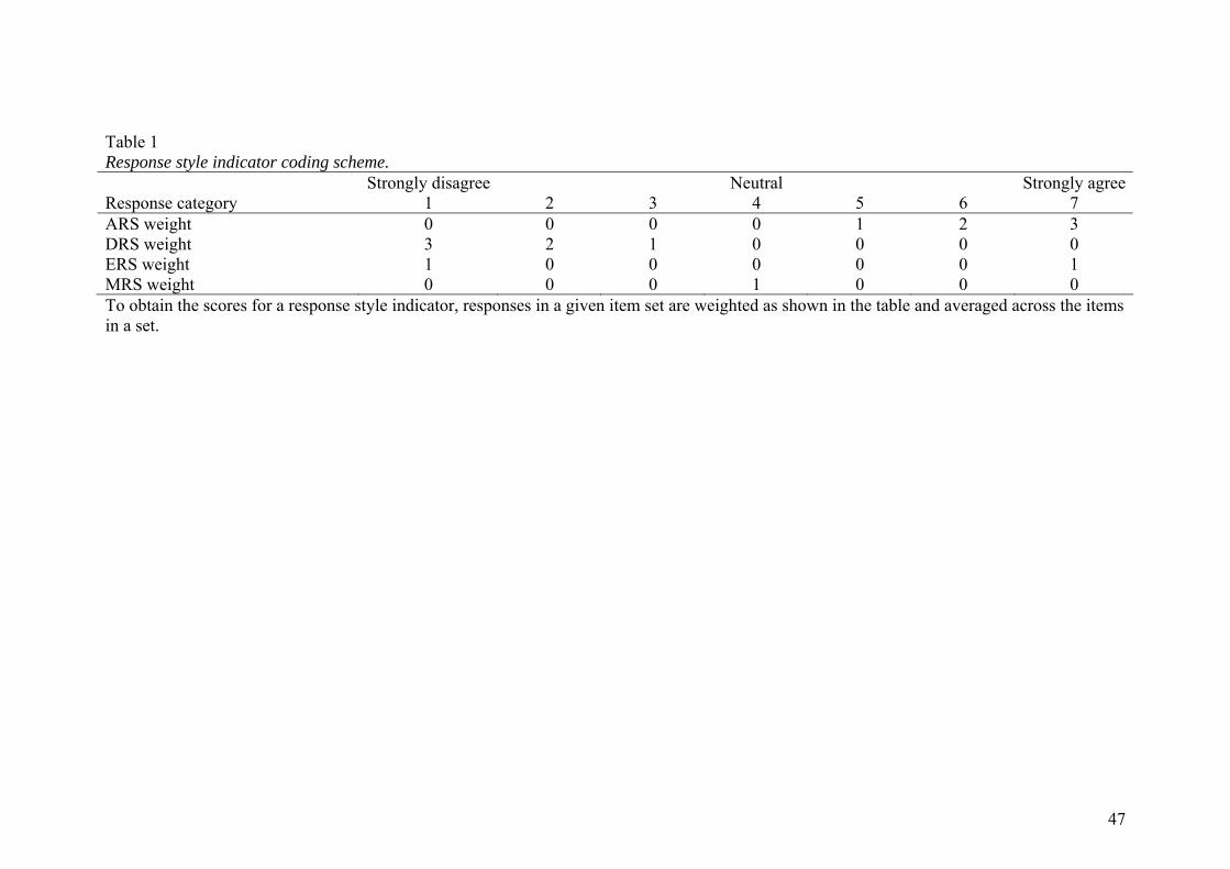
Table 1 Response style indicator coding scheme.

reeRes n or 2 3

Strongpo se categ y

Strongly disag1

Neutral 4 5 6

ly agree 7

ARS iwe g 0 0 0 1 2 ht 0 3 DRS eiw g 2 1 0 0 0

e g 0 0 0 0 0 w g 0 0 1 0 0

ht 3 0 ERS iw ht 1 1 MRS ei ht 0 0 To obtain ores e dicator, responses in a given item set are the sc for a r sponse style in weighted as shown in the table and averaged across the items in a set.

47

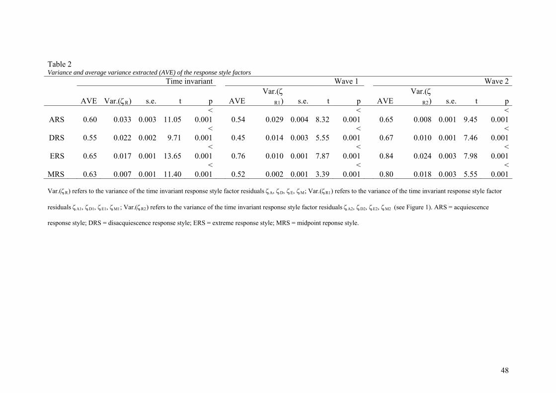
Table 2 Variance and average variance

extracted (AVE) of the response style factors

Time invariant Wave 1 Wave 2

E Va R) s.e. t V s. AVVar.(ζ

R2 s.e. t p AV r.(ζ p A EVar.(ζ

R1) e. t p E )

ARS 0.60 0.033 0.003 11.05 0.54 29 0.004 8.32 0 0 45<

0.001 <

0.001 0.0<

0.001 .65 0.008 .001 9.

DRS 5 22 0 0.45 14 0.003 5.55 0 0 46<

0.001

ERS 0. 17 0 0.76 10 0.001 7.87 0 0.0 98<

0.001

MRS 0.007 0.001 11.40 0.52 0.001 3.39 0 0 55<

0.001

0.5 0.0 .002 <

9.71 0.001 0.0<

0.001 .67 0.010 .001 7.

0.65 0 .001 13.65<

< 0.001 0.0

< 0.001 .84 0.024 03 7.

0.63 0.001 0.002<

0.001 .80 0.018 .003 5. Var.(ζR) refers to the varia e of the or resid ζD, ζE, ζM; Var.(ζR1) ref e varian e tim ria style factor

residuals ζA1, ζD1, ζE1, ζM1 Var.(ζR2) refers to the e invari nse style factor residuals 2, ζE2, ζ Fig AR escence

esponse style; S = di uiescence e respon MRS = midpoint reponse

nc time invariant response style fact uals ζA, ers to th ce of th e inva nt response

; variance of the tim ant respo ζA2, ζD M2 (see ure 1). S = acqui

DR sacq response style; ERS = extrem se style; style. r

48

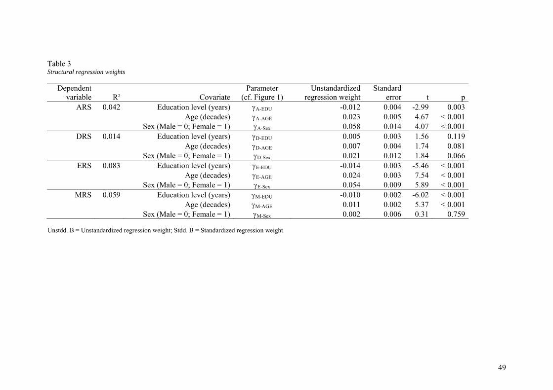
49

Table 3 Structural regression weights

Dependentvariable

Parameter (cf. Figure 1)

Unstandardizedregression weight

Standarderror t p

R² CovariateARS 0.042 γA-EDU -0.012 0.004 -2.99 0.003Education level (years)

Age (decades)Sex (Male = 0; Female = 1)

Education level (years)

γA-AGE 0.023 0.005 4.67 < 0.001 γA-Sex 0.058 0.014 4.07 < 0.001

DRS 0.014 γD-EDU 0.005 0.003 1.56 0.119 Age (decades)

Sex (Male = 0; Female = 1)Education level (years)

γD-AGE 0.007 0.004 1.74 0.081 γD-Sex 0.021 0.012 1.84 0.066

ERS 0.083 γE-EDU -0.014 0.003 -5.46 < 0.001 Age (decades)

Sex (Male = 0; Female = 1)Education level (years)

γE-AGE 0.024 0.003 7.54 < 0.001 γE-Sex 0.054 0.009 5.89 < 0.001

MRS 0.059 γM-EDU -0.010 0.002 -6.02 < 0.001 Age (decades)

Sex (Male = 0; Female = 1)γM-AGE 0.011 0.002 5.37 < 0.001

γM-Sex 0.002 0.006 0.31 0.759 Unstdd. B = Unstandardized r ed regression weight.

egression weight; Stdd. B = Standardiz

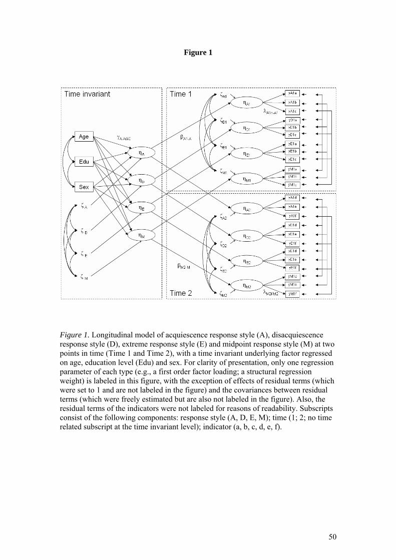
Figure 1

Figure 1. Longitudinal model of acquiescence response style (A), disacquiescence sponse style (D), extreme response style (E) and mre

pidpoint response style (M) at two

oints in time (Time 1 and Time 2), with a time invariant underlying factor regressed on age, education level (Edu) and sex. For clarity of presentation, only one regression parameter of each type (e.g., a first order factor loading; a structural regression weight) is labeled in this figure, with the exception of effects of residual terms (which were set to 1 and are not labeled in the figure) and the covariances between residual terms (which were freely estimated but are also not labeled in the figure). Also, the residual terms of the indicators were not labeled for reasons of readability. Subscripts consist of the following components: response style (A, D, E, M); time (1; 2; no time related subscript at the time invariant level); indicator (a, b, c, d, e, f).

50

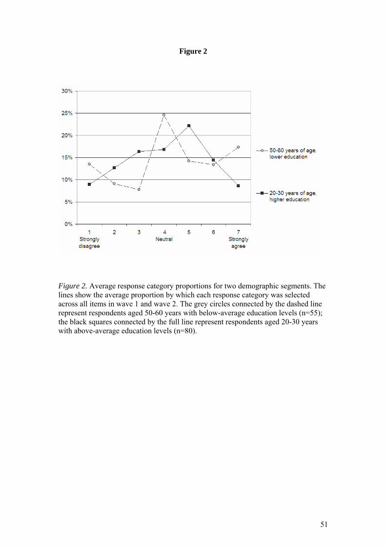
Figure 2

Figure 2. Average response category proportions for two demographic segments. The lines show the average proportion by which each response category was selected

with above-average education levels (n=80).

across all items in wave 1 and wave 2. The grey circles connected by the dashed line represent respondents aged 50-60 years with below-average education levels (n=55); the black squares connected by the full line represent respondents aged 20-30 years

51

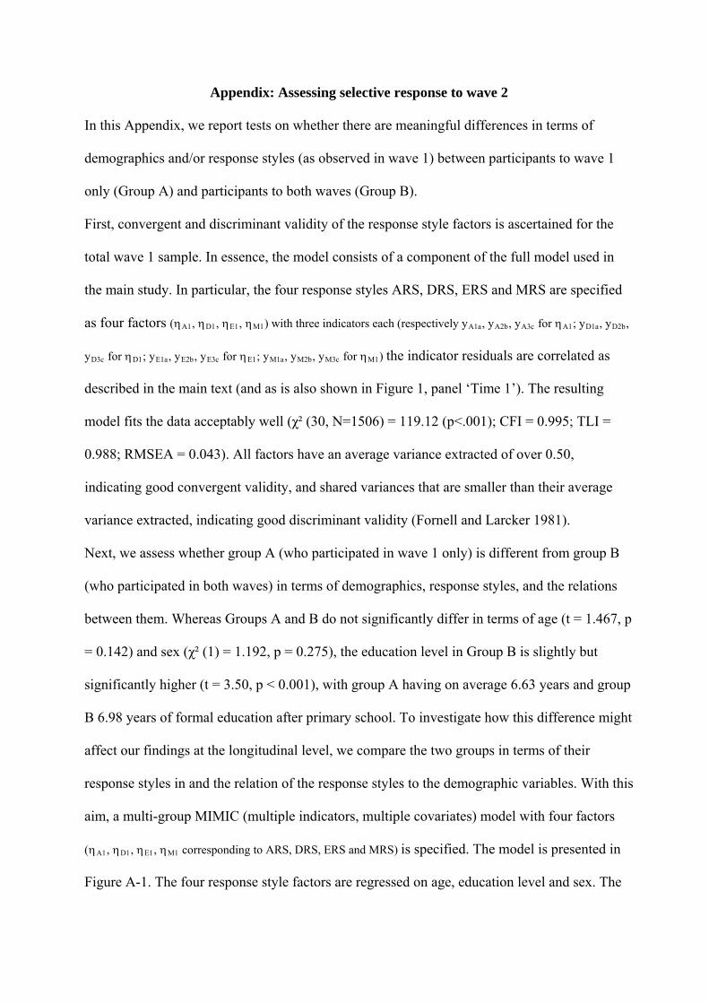
Appendix: Assessing selective response to wave 2

In this Appendix, we report tests on whether there are meaningful differences in terms of

demographics and/or response styles (as observed in wave 1) between participants to wave 1

only (Group A) and participants to both waves (Group B).

First, convergent and discriminant validity of the response style factors is ascertained for the

total wave 1 sample. In essence, the model consists of a component of the full model used in

the main study. In particular, the four response styles ARS, DRS, ERS and MRS are specified

as four factors (ηA1, ηD1, ηE1, ηM1) with three indicators each (respectively yA1a, yA2b, yA3c for ηA1; yD1a, yD2b,

yD3c for ηD1; yE1a, yE2b, yE3c for ηE1; yM1a, yM2b, yM3c for ηM1) the indicator residuals are co elated as

.988; RMSEA = 0.043). All factors have an average variance extracted of over 0.50,

ons

up

difference might

ffect our findings at the longitudinal level, we compare the two groups in terms of their

response styles in and the relation of the response styles to the demographic variables. With this

aim, a multi-group MIMIC (multiple indicators, multiple covariates) model with four factors

(ηA1, ηD1, ηE1, ηM1 corresponding to ARS, DRS, ERS and MRS) is specified. The model is presented in

Figure A-1. The four response style factors are regressed on age, education level and sex. The

rr

described in the main text (and as is also shown in Figure 1, panel ‘Time 1’). The resulting

model fits the data acceptably well (χ² (30, N=1506) = 119.12 (p<.001); CFI = 0.995; TLI =

0

indicating good convergent validity, and shared variances that are smaller than their average

variance extracted, indicating good discriminant validity (Fornell and Larcker 1981).

Next, we assess whether group A (who participated in wave 1 only) is different from group B

(who participated in both waves) in terms of demographics, response styles, and the relati

between them. Whereas Groups A and B do not significantly differ in terms of age (t = 1.467, p

= 0.142) and sex (χ² (1) = 1.192, p = 0.275), the education level in Group B is slightly but

significantly higher (t = 3.50, p < 0.001), with group A having on average 6.63 years and gro

B 6.98 years of formal education after primary school. To investigate how this

a

model is th

parameters is tested.

en simultaneously fit to group A and group B, and invariance of the relevant

Figu ul p IC mod of response styles. The grouping variable

is defined by participation in wave 1 only (group A) in b ve w roup

We first assess in ce e respo e sty ors lu ther t

way across both

roups (Meredith 1993). This turns out to be the case: constraining the measurement weights

C

her

structural weights across both

roups. This also appears to be the case (see model D, E and F in Table A-1).

re A-1. Time specific M ti-grou MIM el

or oth wa 1 and ave 2 (g B).

measurement varian of th ns le fact to eva ate whe he

response style indicators relate to their underlying latent variables in the same

g

(metric invariance) and, subsequently, the measurement intercepts (scalar invariance) to

equality does not lead to a significant or substantial deterioration in fit (see models A, B and

in Table A-1). Using the scalar invariance model as the reference model, we then test whet

the response style factors have equal structural intercepts and

g

53

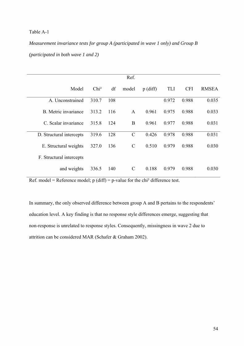
54

Table A-1

Measurement invariance tests for group A (participated in wave 1 only) and Group B

(participated in both wave 1 and 2)

Model Chi² df

Ref.

model p (diff) TLI CFI RMSEA

A. Unconstrained 310.7 108 0.972 0.988 0.035

B. Metric invariance 313.2 116 A 0.961 0.975 0.988 0.033

C. Scalar invariance 315.8 124 B 0.961 0.977 0.988 0.031

D. Structural intercepts 319.6 128 C 0.426 0.978 0.988 0.031

E. Structural weights 327.0 136 C 0.510 0.979 0.988 0.030

F. Structural intercepts

and weights 336.5 140 C 0.188 0.979 0.988 0.030

Ref. model = Reference model; p (diff) = p-value for the chi² difference test.

In summary, the only observed difference between group A and B pertains to the respondents’

education level. A key finding is that no response style differences emerge, suggesting that

non-response is unrelated to response styles. Consequently, missingness in wave 2 due to

attrition can be considered MAR (Schafer & Graham 2002).