The spectrum of genomic signatures: from dinucleotides to chaos game representation

www.elsevier.com/locate/gene

Gene 346 (2005

The spectrum of genomic signatures: from dinucleotides

to chaos game representation

Yingwei Wanga,*, Kathleen Hillb, Shiva Singhb, Lila Karia

aDepartment of Computer Science, University of Western Ontario, London, Ontario, Canada N6A 5B7bDepartment of Biology, University of Western Ontario, London, Ontario, Canada N6A 5B7

Received 8 March 2004; received in revised form 28 September 2004; accepted 21 October 2004

Available online 29 January 2005

Received by A.M. Campbell

Abstract

In the post genomic era, access to complete genome sequence data for numerous diverse species has opened multiple avenues for

examining and comparing primary DNA sequence organization of entire genomes. Previously, the concept of a genomic signature was

introduced with the observation of species-type specific Dinucleotide Relative Abundance Profiles (DRAPs); dinucleotides were identified

as the subsequences with the greatest bias in representation in a majority of genomes. Herein, we demonstrate that DRAP is one

particular genomic signature contained within a broader spectrum of signatures. Within this spectrum, an alternative genomic signature,

Chaos Game Representation (CGR), provides a unique visualization of patterns in sequence organization. A genomic signature is

associated with a particular integer order or subsequence length that represents a measure of the resolution or granularity in the analysis

of primary DNA sequence organization. We quantitatively explore the organizational information provided by genomic signatures of

different orders through different distance measures, including a novel Image Distance. The Image Distance and other existing distance

measures are evaluated by comparing the phylogenetic trees they generate for 26 complete mitochondrial genomes from a diversity of

species. The phylogenetic tree generated by the Image Distance is compatible with the known relatedness of species. Quantitative

evaluation of the spectrum of genomic signatures may be used to ultimately gain insight into the determinants and biological relevance of

the genome signatures.

D 2004 Elsevier B.V. All rights reserved.

Keywords: Dinucleotide Relative Abundance Profiles; Genomic signature distances; Phylogenetic trees; Organizational information of a DNA sequence

1. Introduction

Although efforts are continuously being made toward

understanding the characteristics of genomes, any particular

genome is too long and too complex for a person to directly

comprehend its characteristics. In 1990, Jeffrey proposed

using Chaos Game Representation (CGR) to visualize DNA

primary sequence organization CGR (Jeffrey, 1990). A CGR

0378-1119/$ - see front matter D 2004 Elsevier B.V. All rights reserved.

doi:10.1016/j.gene.2004.10.021

Abbreviations: A, adenosine; C, cytidine; G, guanosine; T, thymidine.

* Corresponding author. Department of Computer Science and Infor-

mation Technology, University of Prince Edward Island, Charlottetown,

Prince Edward Island, C1A 4P3 Canada. Tel.: +1 902 566 0499; fax: +1

902 566 0466.

E-mail address: [email protected] (Y. Wang).

is plotted in a square, the four vertices of which are labelled

by the nucleotides A, C, G, T, respectively. The plotting

procedure can be described by the following steps: the first

nucleotide of the sequence is plotted halfway between the

centre of the square and the vertex representing this

nucleotide; successive nucleotides in the sequence are plotted

halfway between the previous plotted point and the vertex

representing the nucleotide being plotted. The major advant-

age of CGR is the use of a two-dimensional plot to provide a

visual representation of primary DNA sequence organization

for a sequence of any length, including entire genomes.

CGRs of DNA sequences show interesting patterns.

Various geometric patterns, such as parallel lines, squares,

rectangles, and triangles can be found in CGRs. Some of the

CGRs even show a complex fractal geometrical pattern

) 173–185

Y. Wang et al. / Gene 346 (2005) 173–185174

which is very similar to the Sierpinsky Triangle (Mandel-

brot, 1982). These interesting features relevant to the DNA

sequence organization attracted further research in CGR

(Dutta and Das, 1992, Hill et al., 1992, Oliver et al., 1993).

In 1993 Goldman analyzed the patterns shown in CGRs

and concluded that bit is unlikely that CGRs can be more

useful than simple evaluation of nucleotide, dinucleotide

and trinucleotide frequenciesQ (Goldman, 1993). According

to this conclusion, CGR should be relegated to the status of

a pictorial representation of nucleotide, dinucleotide and

trinucleotide frequencies.

After this sobering conclusion, research on CGRs

continued with less frequency. Hill and Singh (1997)

compared CGRs of mitochondrial genomes and explored

the evolution of species-type specificity in DNA sequences.

Almeida et al. (2001) suggested that CGR is a generalization

of Markov Chain probability tables that accommodates non-

integer orders.

In parallel to CGR research, Karlin and Burge proposed

the concept of genomic signature (Karlin and Burge, 1995).

The key observation behind the genomic signature concept

is that Dinucleotide Relative Abundance Profiles (DRAPs)

of different DNA sequence samples from the same organism

are generally much more similar to each other than to those

of sequences from other organisms. In addition, closely

related organisms generally have more similar DRAPs than

distantly related organisms. It was concluded from these

observations that the DRAP values constitute a genomic

signature of an organism.

Since 1995, genomic signatures have been studied from a

variety of perspectives, as witnessed by Karlin et al. (1997),

Campbell et al. (1999), Deschavanne et al. (1999, 2000),

Gentles and Karlin (2001), Sandberg et al. (2001), Edwards

et al. (2002), and Hao et al. (2000). Campbell et al. (1999)

compared genomic signatures of prokaryote, plasmid, and

mitochondrial DNA. Deschavanne et al. (2000) showed that

word usage in short fragments of genomic DNA (as short as

1 kb) is similar to that of the whole genome, thus providing

a strong support to the concept of genomic signature.

Gentles and Karlin (2001) looked at the genomic signature

of various eukaryotes. Sandberg et al. (2001) proposed a

method to classify sequence segments using genomic

signatures. More recently, genomic signatures were used

in phylogenetic analysis (Edwards et al., 2002).

In 1999, an interesting paper provided a link between

CGRs and genomic signatures (Deschavanne et al., 1999).

Experiments showed that variation between CGR images

along a genome was smaller than variation among genomes.

bThese facts strongly support the concept of genomic

signature and qualify the CGR representation as a powerful

tool to unveil itQ (Deschavanne et al., 1999).

In this paper, we discuss CGR and DRAP (currently

proposed as genomic signature) from the following perspec-

tives: In Section 2, we challenge the idea that CGR is merely

a representation of nucleotide, dinucleotide, and trinucleo-

tide frequencies. The aim of Section 2 is to provide evidence

supporting the claim that CGRs have more complex features

worth further investigation. In Section 3, we propose the

idea of a spectrum of genomic signatures, and describe the

common features as well as variations within this spectrum.

Section 4 discusses various distance definitions between

genomic signatures of two DNA sequences. Order is an

integer number associated with a genomic signature to

describe its granularity. In Section 5, we design an experi-

ment to quantitatively analyze the information provided by

the genomic signatures of different orders of a given DNA

sequence. Section 6 presents our conclusions.

2. What determines the pattern in a CGR?

The interesting patterns in CGRs inspired exploration of

the underlying determinants of these patterns in different

ways. Hill et al. (1992) tried to use image analysis

techniques to categorize and analyze CGRs. Goldman

(1993) used Markov Chain model simulation to explore

these determinants.

Goldman (1993) concluded that bthe CGR gives no

further insight into the structure of the DNA sequence than

is given by the dinucleotide and trinucleotide frequenciesQand bunless more complex patterns are found in CGRs,

there is no justification for ascribing their patterns to

anything other than the effects described in this paper.QThese conclusions had the effect that CGRs have sub-

sequently been much less studied from this perspective. In

this section we first present arguments supporting our claim

that CGRs give more insight into DNA structures than those

given by nucleotide, dinucleotide, and trinucleotide fre-

quencies, and then present our answer to the question,

bWhat determines the pattern in a CGR?Q

2.1. Short nucleotide frequencies cannot solely determine

the pattern in a CGR

The results reported in Goldman (1993) are obtained

through DNA sequence simulation based on Markov Chain

model. We first briefly introduce the first-order and

second-order Markov Chain model. In the first-order

Markov Chain model, successive bases in a simulated

sequence depend only on the preceding base. A 4�4

matrix P defines the probabilities with which subsequent

bases follow the current base in a DNA sequence. If the

base labels A, C, G, and T are equated with the numbers 1,

2, 3, and 4, then Pij, the jth element of the ith row of P,

defines the probability that base j follows base i. The row-

sums of P must equal 1. Using this matrix, a simulated

DNA sequence is obtained by selecting a first base

randomly, according to the frequencies of the bases in

the DNA string under study; if this is base i, then the

probabilities Pi1, Pi2, Pi3, and Pi4 are used to select the

next base, and so on until the simulated sequence is of the

same length as the original DNA sequence.

Y. Wang et al. / Gene 346 (2005) 173–185 175

In the second-order Markov Chain model, each base

depends on the previous two bases. All probabilities in the

form of PXYZ, which is the probability that base Z follows

the dinucleotide XY, are used to simulate the original

sequence.

The major result in Goldman (1993) can be described as

follows: For a DNA sequence a, we can construct a

simulated sequence aV using the first-order Markov Chain

model, such that a and aV have the same length and the same

nucleotide and dinucleotide frequencies. We would then

find that the CGRs of a and aV have similar patterns,

suggesting the hypothesis that the patterns in a CGR are

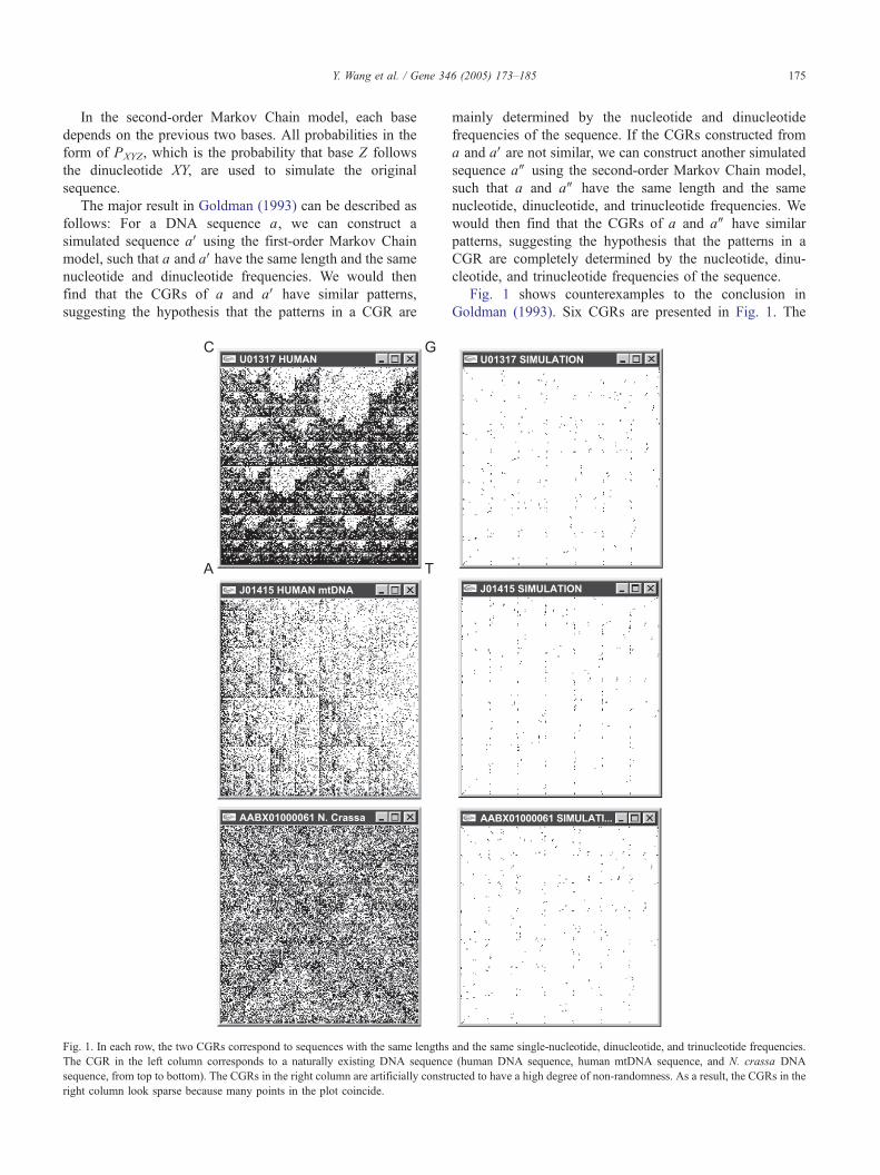
Fig. 1. In each row, the two CGRs correspond to sequences with the same lengths

The CGR in the left column corresponds to a naturally existing DNA sequence

sequence, from top to bottom). The CGRs in the right column are artificially constr

right column look sparse because many points in the plot coincide.

mainly determined by the nucleotide and dinucleotide

frequencies of the sequence. If the CGRs constructed from

a and aV are not similar, we can construct another simulated

sequence aW using the second-order Markov Chain model,

such that a and aW have the same length and the same

nucleotide, dinucleotide, and trinucleotide frequencies. We

would then find that the CGRs of a and aW have similar

patterns, suggesting the hypothesis that the patterns in a

CGR are completely determined by the nucleotide, dinu-

cleotide, and trinucleotide frequencies of the sequence.

Fig. 1 shows counterexamples to the conclusion in

Goldman (1993). Six CGRs are presented in Fig. 1. The

and the same single-nucleotide, dinucleotide, and trinucleotide frequencies.

(human DNA sequence, human mtDNA sequence, and N. crassa DNA

ucted to have a high degree of non-randomness. As a result, the CGRs in the

Y. Wang et al. / Gene 346 (2005) 173–185176

three CGRs from the left column (top to bottom) are

plotted from a human DNA sequence, a human mtDNA

sequence, and a Neurospora crassa DNA sequence,

respectively (GenBank accession number:U01317,J01415,

and AABX01000061). The three CGRs from the right

column are plotted from sequences constructed by simulat-

ing the length and the single-nucleotide, dinucleotide, and

trinucleotide frequencies of the corresponding sequences in

the left column. The striking point supporting our claim is

that the corresponding CGRs in these two columns are not

similar at all.

How could this happen? The reason is that the sequences

shown in the right column are constructed by simulating the

sequences shown in the left column using an algorithm other

than the Markov Chain model. While we do not go into the

details of the algorithm that constructed these sequences, we

use the following example to illustrate the idea behind it.

Suppose we have sequences X, Y, and Z, where Sequence X

is a segment of the human genome and Sequences Y and Z

are constructed by simulating X.

X : GATCACAGGTCTATCACCCTATTAACCACT-

CACGGGAGCT

Y: AAAAAAAAAAACCCCCCCCCCCCCGGGGGG-

TTTTTTTTT

Z: AACACACACACAGAGATATATCCCGCTCTCTC-

TCGGGGTT

We can verify that Sequence Y has the same single

nucleotide frequencies as Sequence X. Sequence Z has both

the same single nucleotide frequencies and similar dinucleo-

tide frequencies as Sequence X. We also notice that the

nucleotides in Sequence Y and Sequence Z are highly non-

randomly arranged.

Because of this non-randomness, the CGRs of Sequence

Y and Sequence Z have many points that coincide so that

these CGRs blookQ very sparse.

Although the sequences shown in the right column of

Fig. 1 are constructed for illustration purposes, and such

sequences of this length (more than 16,000 bases) can

hardly exist in natural DNA genomes, Fig. 1 clearly shows

that a sequence’s nucleotide, dinucleotide, and trinucleotide

frequencies cannot solely determine its CGR pattern.

2.2. What determines the pattern in a CGR?

Fig. 1 shows that a CGR contains more information than

nucleotide, dinucleotide, and trinucleotide frequencies. The

next question is what determines the pattern in a CGR?

Suppose a DNA sequence has been plotted in a CGR,

and the size of the CGR is 1�1. We divide the CGR by a

2k�2k grid. According to the characteristics of a CGR, each

grid square corresponds to a length k oligonucleotide, and

the number of points within a grid square is the number of

occurrences of the corresponding length k oligonucleotide

in this DNA sequence. The length k�1 oligonucleotide at

the beginning of the DNA sequence corresponds to points

on the grid lines instead of inside any grid square. If the

DNA sequence is much longer than k, we can omit these

k�1 points.

A practical CGR medium, such as paper, screen, or

memory space, always has a limited resolution. If the

resolution of a CGR is 1/2k and we divide the CGR by a

2k�2k grid, we cannot distinguish points inside a same grid

square. We may paint a whole grid square with a gray scale

to express the number of points in the grid square: The more

points in the grid square, the darker the shade of grey.

To conclude, if a CGR’s resolution is 1/2k and the DNA

sequence is much longer than k, this CGR is completely

determined by all the length k oligonucleotide occurrences

or frequencies. These frequencies reveal all the information

in a CGR.

The above discussion suggests another method of plotting

a CGR: Suppose we want to plot a DNA sequence in a CGR

on a media, and the resolution of this media is 1/2k. In other

words, the image area in this media is divided into 2k�2k

squares. We first count the number of occurrences for each

length k oligonucleotide in this DNA sequence. Then we

paint each square with a proper shade of gray according to

the number of occurrences of the corresponding length k

oligonucleotide in this DNA sequence.

If k=3, the CGR is totally determined by nucleotide,

dinucleotide, trinucleotide frequencies, and the conclusions

in Goldman (1993) are correct. However, if kN3, a CGR

cannot be totally determined by nucleotide, dinucleotide,

and trinucleotide frequencies. Longer oligonucleotide fre-

quencies may influence the pattern of the CGR. Fig. 1

shows that sometimes longer oligonucleotide frequencies

may have a big impact on the CGR pattern.

To summarize, the contribution of Goldman (1993) was

that it introduced the Markov Chain model to simulate a

sequence. The CGRs of sequences simulated this way

indicated that nucleotide, dinucleotide and trinucleotide

frequencies are able to produce the patterns in CGRs. We

claim that, while it is true that nucleotide, dinucleotide and

trinucleotide frequencies are able to influence the patterns in

CGRs, it was erroneous to conclude that these frequencies

can solely determine the patterns in CGRs. However, we

believe that under a different interpretation, the Markov

Chain model can still prove to be useful, and we will use the

Markov Chain model again in Section 5.

3. A spectrum of genomic signatures

3.1. FCGR (the Frequency matrix extracted from a CGR)

and DRAP

Both DRAP and CGR have been proposed as genomic

signatures. Before we examine the relationship between

these two kinds of genomic signatures, we first discuss their

definitions to clarify any ambiguity.

Y. Wang et al. / Gene 346 (2005) 173–185 177

For a sequence s, the dinucleotide relative abundance

profile DRAP(s) is an array {qXY=fXY/fXfY}, where XY

stands for all possible dinucleotide combinations, fX denotes

the frequency of the mononucleotide X in s and fXY the

frequency of the dinucleotide XY in s. We use sV to denote

the reverse complement of s. DRAP(ssV) is the dinucleotiderelative abundance profile computed from the sequence s

concatenated with its reverse complement sV.CGRs in their original form are not convenient to be

processed by a computer. Thus, we introduce another form

of CGR: FCGR. The structure of FCGR was introduced in

Deschavanne et al. (1999) and the name FCGR was

proposed in Almeida et al. (2001). For convenience, in this

paper, we introduce the concept of order of a FCGR and

define a kth-order FCGR as follows.

A kth-order FCGR of a sequence s, denoted by

FCGRk(s), is a 2k�2k matrix. To obtain this FCGR, we

first plot a CGR from s, then divide this CGR by a 2k�2k

grid so that each grid square corresponds to an element in

the matrix, count the number of points inside each grid

square, and use the number of points as the matrix element

corresponding to the grid square. We do not count those

points on the grid square lines because they represent the

length k�1 oligonucleotide at the beginning of the DNA

sequence, and we can omit these k�1 points as long as the

DNA sequence is much longer than k. Note that, instead of

being a graphical representation like CGR, a FCGR is a

numerical matrix.

A FCGR can also be constructed directly from a

sequence instead of plotting a CGR first and then converting

the CGR into a FCGR. We can construct a FCGR directly

by counting the number of occurrences of each length k

oligonucleotide in the sequence and putting this number into

the appropriate place of the FCGR matrix, according to the

correspondence between a length k oligonucleotide and a

CGR grid square.

A first-order FCGR and a second-order FCGR have the

structure shown below, where Nw is the number of

occurrences of the oligonucleotide w in the sequence s.

FCGR1 sð Þ ¼ NC NG

NA NT

��

FCGR2 sð Þ ¼

NCC NGC NCG NGG

NAC NTC NAG NTG

NCA NGA NCT NGT

NAA NTA NAT NTT

1CCA

0BB@

The definition of FCGRk+1(s) can be obtained by

replacing each element NX in FCGRk(s) with four elements

NCX NGX

NAX NTX

A kth-order FCGR can also be applied to a sequence

concatenated with its reverse complement, and such a

FCGR is described as FCGRk(ssV).

If we have a CGR of resolution 1/2k, we can transform

the gray shade of each square into a number, and obtain a

kth-order FCGR; If we have a kth-order FCGR, we can plot

a CGR of resolution 1/2k according to the method

introduced in Section 2. In conclusion, a kth-order FCGR

is equivalent to a CGR of resolution 1/2k.

A kth-order FCGR contains 4k numbers of length k

oligonucleotide occurrences. If k=5, 4k is over one

thousand; if k=10, 4k is over one million. It is almost

impossible for a person to comprehend the significance of

so many numbers at one time. Because a kth-order FCGR is

equivalent to a CGR of resolution 1/2k, one can comprehend

the major features present in the large number of elements in

the FCGR matrix by visually checking the equivalent CGR

of resolution 1/2k.

Finally, the relationship between DRAPs and 2nd-order

FCGRs is that DRAPs are deducible from 2nd-order FCGRs

but 2nd-order FCGRs are not deducible from DRAPs.

3.2. A spectrum of genomic signatures

Both second-order FCGR and DRAP have 16 elements,

and each element corresponds to one dinucleotide. An

element of a second-order FCGR involves only the

frequency of the dinucleotide. On the contrary, as the name

brelative abundanceQ suggests, an element of a DRAP is the

ratio of the dinucleotide frequency to the frequencies of the

two single nucleotides composing this dinucleotide. We call

an element of a DRAP a relative frequency. Thus, we may

call DRAP a second-order relative FCGR, and denote it as

rFCGR2(s).

rFCGR2 sð Þ ¼

�CC �GC �CG �GG�AC �TC �AG �TG�CA �GA �CT �GT�AA �TA �AT �TT

1CCA

0BB@

Normally, in a DRAP, all the elements are organized in

an array; in a second-order relative FCGR the same

elements are organized in a matrix. Organizing the elements

of a DRAP as a second-order relative FCGR not only

reveals the similarity of a DRAP and a FCGR, but also

enables us to define a kth-order relative FCGR (kz2).

By expanding the definition of a DRAP, we can define

a trinucleotide relative abundance profile as {qXYZ=fXYZ/

fX fY fZ} for all trinucleotides XYZ, and further define even

longer oligonucleotide relative abundance profiles in the

same way. Similarly, we can express a trinucleotide

relative abundance profile as a 3rd-order relative FCGR.

In the general situation, we can express a length k

oligonucleotide relative abundance profile as a kth-order

relative FCGR. These relative FCGRs can also be

visualized in a CGR.

Based on these discussions, we propose the idea that

various kinds of genomic signatures exist, and they can be

considered as members of a spectrum of genomic signa-

tures. All genomic signatures in the spectrum have some

Y. Wang et al. / Gene 346 (2005) 173–185178

common features: each genomic signature is a numerical

matrix and can be visualized in a CGR; a positive integer

number called order determines its granularity; if the order

is k, the numerical matrix has 2k�2k elements. Each element

in the matrix is mapped to a length k oligonucleotide as

described in the definition of FCGR.

For now, we know that the spectrum of genomic

signatures contains two major categories: FCGR and

relative FCGR. Note that a second-order relative FCGR is

equivalent to a DRAP. Besides choosing FCGR or relative

FCGR, other choices also determine the variations in the

spectrum of genomic signatures.

One choice is about whether we concatenate the DNA

sequence with its reverse complement before we count the

frequencies. By concatenating a DNA sequence with its

reverse complement we eliminate some unnecessary biases

in the sequence. In the original definition of a DRAP, a

DNA sequence is always concatenated with its reverse

complement before the frequencies are counted, but this is

not the only choice. When we construct a FCGR or a

relative FCGR, we can either concatenate the DNA

sequence with its reverse complement or not do so.

Another issue concerns the standardization of FCGRs.

The sum of all elements in a FCGR is proportional to the

length of the DNA sequence in question. Because a genomic

signature is supposed to be only associated with a species,

we need to eliminate the factor of DNA sequence length

from FCGRs so that we are able to compare the FCGRs

obtained from DNA sequences of different lengths and

further explore the usefulness of FCGRs. The procedure of

eliminating the sequence length parameter from the FCGR

definition, called herein standardization, will be described in

the sequel.

Suppose A is a kth-order FCGR. We know A is a

2k�2k matrix, and we use ai, j (1V i V 2k, 1V jV 2k) to

denote the elements in this matrix. We can standardize A,

and the standardized FCGR, denoted by A, is defined as

follows:

AA ¼ 4kPi

Pj ai; j

A

Assuming that the elements in A are denoted by bi, j, we

have the following property:

X2ki¼1

X2kj¼1

bi; j ¼ 4k

This property means that in a standardized kth-order

FCGR, the sum of all elements equals the number of

elements, and therefore the average value of the elements of

the matrix is 1.

Being sequence length independent, standardized FCGRs

are thus preferable when comparing genomes of different

organisms. Non-standardized FCGRs could still be useful

for other reasons. For example, we can plot a CGR of

resolution 1/2k from a non-standardized kth-order FCGR,

but we cannot plot a CGR from a standardized kth-order

FCGR.

To conclude, in this section, we have presented the

common features of and variations within the spectrum of

genomic signatures. We conjecture that different genomic

signatures could be used for different purposes.

4. The distance between genomic signatures of two DNA

sequences

A distance between the genomic signatures of two DNA

sequences is an important measure in evaluating the

difference between them. Such a distance measure can be

used, for example, in phylogenetic analysis.

There are many different ways to define such a distance

measure. Different distance definitions have different

features and can serve different purposes.

4.1. Geometric distances

According to geometry, we can define the Euclid

distance and Hamming distance between two points in a

multi-dimensional space. We may consider a 2k�2k matrix

as a point in a 4k-dimensional space, and define the Euclid

distance and Hamming distance as follows:

Definition 1 (Euclid distance). Let us assume that matrices

A=(a)2�2k and B=(b)2k�2k are standardized kth-order

FCGRs. We define the Euclid distance between A and B as:

dE AA; BB� �

¼ffiffiffiffiffi2k

p

4k

ffiffiffiffiffiffiffiffiffiffiffiffiffiffiffiffiffiffiffiffiffiffiffiffiffiffiffiffiffiffiffiffiffiffiffiffiffiffiffiffiffiX2ki¼1

X2kj¼1

ai; j � bi; j� �2

vuut

The constant

ffiffiffiffi2k

p4k

is used to adapt the standard Euclid

distance so that the distance values for different k values will

be in the same range. We omit the detailed discussion about

why this constant should be

ffiffiffiffi2k

p4k

; briefly speaking, this

constant is related to the definition of a standardized FCGR.

Definition 2 (Hamming distance). Let us assume that

matrices A=(a)2k�2k and B=(b)2k�2k are standardized kth-

order FCGRs. We define the Hamming distance between A

and B as:

dH AA; BB� �

¼ 1

4k

X2ki¼1

X2kj¼1

jai; j � bi; jj

Campbell et al. (1999) suggested that for two sequences f

and g, the distance between two DRAPs should be defined

as

d f ; gð Þ ¼ 1=16XXY

jqXY fð Þ � qXY gð Þj

As it turns out, this DRAP distance is a special case of

the Hamming distance.

Y. Wang et al. / Gene 346 (2005) 173–185 179

As we observed, there are several ways in which one can

define the distance between two FCGRs. One of the

desirable properties of such a distance would be that the

distance between two DNA sequences of the same genome

should be small. The Hamming distance satisfies this

property for DRAP and low-order FCGRs (kV3). However,for higher-order (kN7) FCGRs, the Hamming distance could

be pretty big, close to the maximum distance value, because

longer oligonucleotide frequencies are not always stable. In

these cases, the Hamming distance loses its discrimination

power.

We will define in the following another distance to

measure the similarity between two FCGRs, according to

the image similarity between the two CGRs visualized from

these FCGRs. This distance is called Image distance, and it

is an expansion of the Hamming distance concept.

The following definitions are needed to define the Image

distance.

Definition 3 (Neighborhood). Suppose we have a matrix

A=(a)n�n, a positive integer R, and a pair (i, j) where 1V i,jVn. A neighborhood of radius R, centered at (i,j), denoted

as HR(i, j), consists of all integer pairs (s,t), where 1Vs V n,

1V tVn, sa[i�R,i+R], and ta[ j�R, j+R].

Definition 4 (Density). For a matrix A=(a)n�n, we define a

density matrix (densityR(A))n�n, where for any (i, j), 1Vi V n,

1V jVn

densityR Að Þi; j ¼P

s;tð ÞaHR i; jð Þ as;tPs;tð ÞaHR i; jð Þ 1

Now we define the Image distance between two FCGRs:

Definition 5 (Image distance). Let us assume that matrices

A=(a)2k�2k and B=(b)2k�2k are standardized kth-order

FCGRs. We define the Image distance between A and B as:

dIR AA; BB� �

¼ 1

4k

X2ki¼1

X2kj¼1

���densityR AA� �

i; j� densityR BB

� �i; j

���

In the above definition, the Image distance is related to

the neighborhood radius R. If R=0, densityR(A)i, j=ai, j and

thus dI0(A,B) is the Hamming distance of two FCGRs. If

RN0, the frequency values within the neighborhood are

averaged in the distance computation. The value of R can be

chosen by a trial-and-error method so that the distance

values fit a specific purpose.

The following formula gives an upper bound of the

maximum Image distance value for a specific R (we omit

the proof):

dIR AA; BB� �

V22Rþ 1

Rþ 1

� �2

:

4.2. Statistical distance

According to statistics, the distance between two sets of

samples can be obtained by calculating the Pearson’s

correlation coefficient between these two sets of samples.

We may consider a 2k�2k matrix as a set of samples, and

define a distance measure accordingly. Almeida et al.

(2001) suggested that the distance between two FCGRs

could be based on a slightly modified Pearson’s correlation

coefficient.

Definition 6 (Pearson distance). Suppose FCGR A is

expressed as an array (xi)(1ViVn), and FCGR B is expressed

as an array ( yi)(1ViVn). The Pearson distance dP(A,B) can be

defined through the following steps:

nw ¼Xni¼1

xidyi xxw ¼

Xni¼1

x2i d yi

nwyyw ¼

Xni¼1

xid y2i

nw

sx ¼

Xni¼1

xi � xxwð Þ2d xid yinw

sy ¼

Xni¼1

yi � yywð Þ2d xid yinw

rwx;y ¼

Xni¼1

xi � xxwffiffiffiffisx

p dyi � yywffiffiffiffi

syp d xid yi

nwdP A;Bð Þ ¼ 1� rwx;y

One advantage of the Pearson distance is that we do not

need to standardize FCGR matrices before the distance

calculation.

4.3. Evaluation of distances

It is difficult to conclude that one distance measure is

better than the others because different distance definitions

have different features and can serve different purposes.

Here we just evaluate these distance definitions from a

specific perspective: generating phylogenetic trees.

We chose 26 mitochondrial DNA sequences; each

sequence is from a specific organism. These sequences are

described in Table 1.

We construct a 10th-order FCGR for each sequence. For

each distance definition, we calculate the distances among

all these FCGRs. We notice that for the Hamming distance,

most of the distance values are close to the maximum

Hamming distance value, showing that when the order is 10,

the Hamming distance cannot properly discriminate FCGRs.

Thus, we do not use the Hamming distance in the next step.

After excluding the Hamming distance, we use the

software package PHYLIP to generate phylogenetic trees

from the distance matrices corresponding to the Euclid

distance, Image distance, and Pearson distance, respectively.

Due to space limitation, we omit the distance data and

just show the phylogenetic trees obtained by this method in

Fig. 2(a), (b), and (c). As a term of reference, we also use

CLUSTALW to directly generate a phylogenetic tree for

these 26 sequences, shown in Fig. 2(d). By checking the

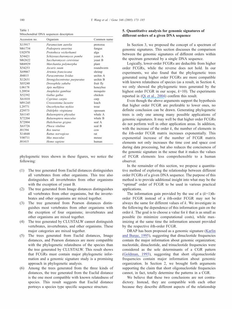
Table 1

Mitochondrial DNA sequences description

Accession no. Organism Common name

X15917 Paramecium aurelia protozoa

M61734 Podospora anserina fungus

U02970 Prototheca wickerhamii alga

X54421 Schizosaccharomyces pombe yeast A

M62622 Saccharomyces cerevisiae yeast B

M68929 Marchantia polymorpha plant

X54253 Ascaris suum roundworm

X69067 Artemia franciscana shrimp

J04815 Paracentrotus lividus urchin A

X12631 Strongylocentrotus purpuratus urchin B

X03240 Drosophila yakuba fruit fly

L06178 Apis mellifera honeybee

L20934 Anopheles gambiae mosquito

X52392 Gallus gallus chicken

X61010 Cyprinus carpio carp

M91245 Crossostoma lacustre loach

L29771 Oncorhynchus mykiss trout

Z29573 Didelphis virginiana opossum

X61145 Balaenoptera physalus whale A

X72204 Balaenoptera musculus whale B

X72004 Halichoerus grypus seal A

X63726 Phoca vitulina seal B

J01394 Bos taurus cow

X14848 Rattus norvegicus rat

V00711 Mus musculus mouse

J01415 Homo sapiens human

Y. Wang et al. / Gene 346 (2005) 173–185180

phylogenetic trees shown in these figures, we notice the

following:

(1) The tree generated from Euclid distances distinguishes

all vertebrates from other organisms. This tree also

distinguishes all invertebrates from other organisms

with the exception of yeast B.

(2) The tree generated from Image distances distinguishes

all vertebrates from other organisms, but the inverte-

brates and other organisms are mixed together.

(3) The tree generated from Pearson distances distin-

guishes most vertebrates from other organisms with

the exception of four organisms; invertebrates and

other organisms are mixed together.

(4) The tree generated by CLUSTALW cannot distinguish

vertebrates, invertebrates, and other organisms. These

major categories are mixed together.

(5) The trees generated from Euclid distances, Image

distances, and Pearson distances are more compatible

with the phylogenetic relatedness of the species than

the tree generated by CLUSTALW. This result shows

that FCGRs must contain major phylogenetic infor-

mation and a genomic signature study is a promising

approach in phylogenetic analysis.

(6) Among the trees generated from the three kinds of

distances, the tree generated from the Euclid distance

is the one most compatible with known relatedness of

species. This result suggests that Euclid distance

portrays a species type specific sequence structure.

5. Quantitative analysis for genomic signatures of

different orders of a given DNA sequence

In Section 3, we proposed the concept of a spectrum of

genomic signatures. This section discusses the comparison

between the genomic signatures of different orders within

the spectrum generated by a single DNA sequence.

Logically, lower-order FCGRs are deducible from higher

order FCGRs, while the reverse does not hold. In our

experiments, we also found that the phylogenetic trees

generated using higher order FCGRs are more compatible

with known relatedness of species (as a result, in Section 4,

we only showed the phylogenetic trees generated by the

highest order FCGR in our scope, k=10). The experiments

reported in (Qi et al., 2004) confirm this result.

Even though the above arguments support the hypothesis

that higher order FCGR are preferable to lower ones, no

definite conclusion can be drawn. Generating phylogenetic

trees is only one among many possible applications of

genomic signatures. It may well be that higher order FCGRs

do not perform well in other application areas. In addition,

with the increase of the order k, the number of elements in

the kth-order FCGR matrix increases exponentially. This

exponential increase of the number of FCGR matrix

elements not only increases the time cost and space cost

during data processing, but also reduces the conciseness of

the genomic signature in the sense that it makes the values

of FCGR elements less comprehensible to a human

observer.

In the remainder of this section, we propose a quantita-

tive method of exploring the relationship between different

order FCGRs of a given DNA sequence. The purpose of this

method is to provide additional insight into what may be the

boptimalQ order of FCGR to be used in various practical

applications.

The information gain provided by the use of a (k+1)th-

order FCGR instead of a kth-order FCGR may not be

always the same for different values of k. We investigate in

the following the dependence of this information gain on the

order k. The goal is to choose a value for k that is as small as

possible (to minimize computational costs), while max-

imizing at the same time the information amount provided

by the respective kth-order FCGR.

DRAP has been proposed as a genomic signature (Karlin

and Burge, 1995), suggesting that dinucleotide frequencies

contain the major information about genomic organization;

nucleotide, dinucleotide, and trinucleotide frequencies were

considered as the sole determinants of a CGR pattern

(Goldman, 1993), suggesting that short oligonucleotide

frequencies contain major information about genomic

organization. In Section 2, we brought forth arguments

supporting the claim that short oligonucleotide frequencies

cannot, in fact, totally determine the patterns in a CGR.

We believe that these two conclusions are not contra-

dictory. Instead, they are compatible with each other

because they describe different aspects of the relationship

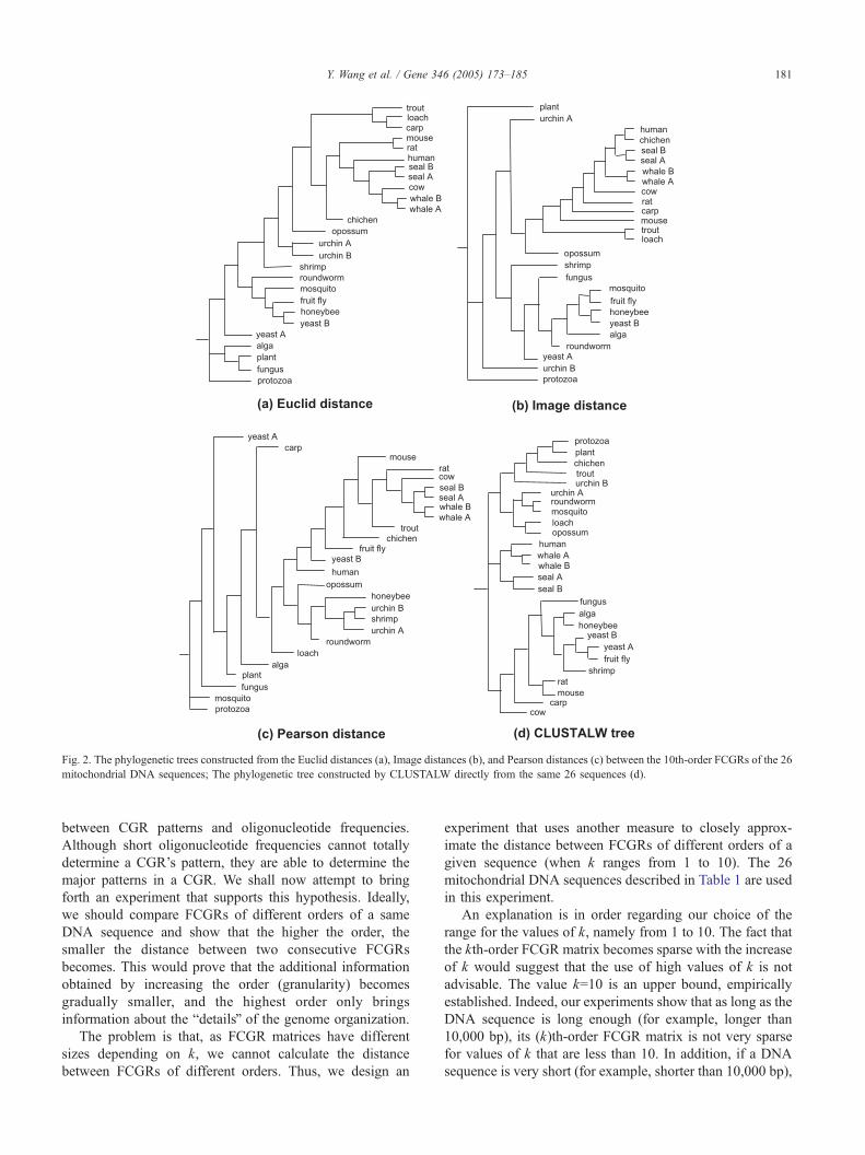
Fig. 2. The phylogenetic trees constructed from the Euclid distances (a), Image distances (b), and Pearson distances (c) between the 10th-order FCGRs of the 26

mitochondrial DNA sequences; The phylogenetic tree constructed by CLUSTALW directly from the same 26 sequences (d).

Y. Wang et al. / Gene 346 (2005) 173–185 181

between CGR patterns and oligonucleotide frequencies.

Although short oligonucleotide frequencies cannot totally

determine a CGR’s pattern, they are able to determine the

major patterns in a CGR. We shall now attempt to bring

forth an experiment that supports this hypothesis. Ideally,

we should compare FCGRs of different orders of a same

DNA sequence and show that the higher the order, the

smaller the distance between two consecutive FCGRs

becomes. This would prove that the additional information

obtained by increasing the order (granularity) becomes

gradually smaller, and the highest order only brings

information about the bdetailsQ of the genome organization.

The problem is that, as FCGR matrices have different

sizes depending on k, we cannot calculate the distance

between FCGRs of different orders. Thus, we design an

experiment that uses another measure to closely approx-

imate the distance between FCGRs of different orders of a

given sequence (when k ranges from 1 to 10). The 26

mitochondrial DNA sequences described in Table 1 are used

in this experiment.

An explanation is in order regarding our choice of the

range for the values of k, namely from 1 to 10. The fact that

the kth-order FCGR matrix becomes sparse with the increase

of k would suggest that the use of high values of k is not

advisable. The value k=10 is an upper bound, empirically

established. Indeed, our experiments show that as long as the

DNA sequence is long enough (for example, longer than

10,000 bp), its (k)th-order FCGR matrix is not very sparse

for values of k that are less than 10. In addition, if a DNA

sequence is very short (for example, shorter than 10,000 bp),

Y. Wang et al. / Gene 346 (2005) 173–185182

we cannot obtain a stable genomic signature regardless of the

value of k. This made k=10 a good empirical choice for the

upper bound of the order of the FCGR.

The measure defined to approximate the distance

between the FCGRs of different orders of the same DNA

sequence is constructed as follows. For each sequence s

and each number k between 1 and 10, we construct a

simulated sequence sV. The new sequence sV has the same

length and the same (or very similar) kth-order FCGR with

the original sequence s, similarity achieved by using the

(k�1)th-order Markov Chain model in which each base

depends on the previous (k�1) bases. We claim that the

randomness in the construction of sV, together with the

mentioned restriction, ensure that the Image distance

between the 10th-order FCGRs of s and sV closely

approximates the distance between the 10th-order FCGR

and the kth-order FCGR of s. We shall thus use in our

analysis the former computable quantity to represent the

latter uncomputable one.

We now formally describe the above procedure. We use

L(s) to denote the length of the sequence s and sim(A,L) to

denote the length L sequence constructed by simulating a

FCGR A. For a specific sequence s and an integer k, we

calculate the following Image distance:

dI20 FCGR10 sð Þ;FCGR10 sim FCGRk sð Þ; L sð Þð Þð Þð Þ � 1000

ð1Þ

Several practical observations are in order. Our experi-

ments suggest that R=20 is a good neighborhood radius

choice for the Image distance calculation between two 10th-

order FCGRs. By multiplying in Eq. (1) the distance by

1000, we need only deal with integer numbers instead of

decimal numbers. Finally, according to the last formula of

Section 4.1, the upper bound for the above distance is 7624.

Why do we think the distance defined in Eq. (1)

accurately describes the difference between the 10th-order

FCGR and the kth-order FCGR of the DNA sequence s?

This is, after all, a distance between two different sequences,

the 1st one being the original sequence, and the 2nd one

being constructed by a (k�1)th-order Markov Chain model

to simulate the kth-order FCGR of the original sequence.

We claim that the 2nd sequence, sim(FCGRk(s),L(s)),

brepresentsQ in some sense the kth-order FCGR of s. Indeed,

the simulated sequence is constructed as randomly as

possible using the model described, with the only restriction

that its kth-order FCGR is the same with the kth-order

FCGR of the original sequence s. Any additional restriction

on the organization of the 2nd sequence would influence its

higher-than-kth-order frequencies, and thus is not desirable.

The randomness of the construction ensures that the 2nd

sequence bdescribesQ the kth-order FCGR of s and thus, the

distance in Eq. (1) is bequivalentQ in some sense to the

distance

dI20 FCGR10 sð Þ; FCGRk sð Þð Þ � 1000 ð2Þ

which we intend to analyze. Consequently, we shall use in

the sequel the computable quantity (Eq. (1)) to represent the

uncomputable quantity (Eq. (2)). For purposes of clarity, we

will abbreviate in the remainder of this section both of these

closely related quantities by

dFCGR 10; kð Þ sð Þ ð3Þ

Let us examine now the results of our computational

experiments, summarized numerically in Table 2 and

graphically in Fig. 3. For each value of k, we have a

column of 26 distances dFCGR(10,k)(s) where s ranges over

the 26 mitochondrial DNA sequences analyzed. To describe

the general tendency and variation of these data sets

(columns) we can use statistical measures, such as average

and standard deviation. In this experiment, because we are

only concerned with those distances that are larger than the

average distance, we use the difference between the

maximum distance and the average distance instead of the

standard deviation to describe the variation within a set

(column). These two measures, the average distance and the

difference between the maximum distance and the average

distance, describe the general behaviour of all the 26

distances.

In Table 2 and Fig. 3, we observe that:

(1) Using higher-order FCGRs will add information about

the DNA sequence that originated them (albeit at a

slower pace). This is illustrated in Table 2 and Fig. 3.

For example, the average distance between the 10th-

order FCGR and the 2nd-order FCGR (221) is twice

the average distance between the 10th-order FCGR and

the 5th-order FCGR (109). This signifies an increase of

information gain for increased k, as witnessed by the

decrease in the difference (from 221 to 109) between

the information content of the kth-order approximation

and the maximum information content available about

the DNA sequence at hand (herein achieved for k=10,

the maximum order in our range). However, the price

paid for this information gain is that the number of

elements in the FCGR matrix increases from 16 to

1024 when k increases from 2 to 5. For modern

computers, the time cost and space cost for 1024

elements are not an issue. However, while a human

observer may be able to check the 16 elements of a

2nd-order FCGR and interpret their meanings as

occurrences of dinucleotide DNA sequences, the same

observer would unable to do the same for a 1024-

element matrix. To summarize, a higher-order FCGR

does indeed provide more information than a lower-

order FCGR, but the extra information is not always

large enough to justify its use, considering that the

price is a significant loss in the bconcisenessQ of theFCGR. The user may tradeoff among these factors

according to the concrete application at hand.

(2) The average of the distances dFCGR(10,k)(s) (com-

puted over the set of the 26 mitochondrial DNA

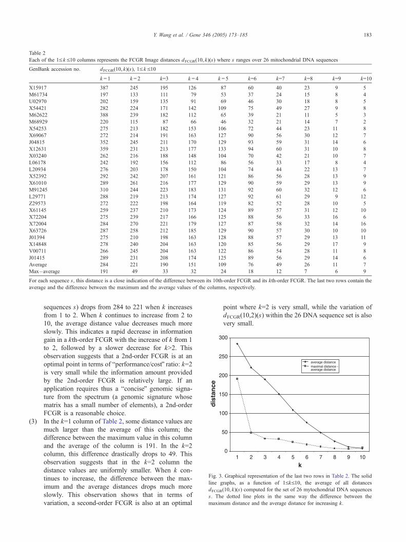
Table 2

Each of the 1V k V10 columns represents the FCGR Image distances dFCGR(10, k)(s) where s ranges over 26 mitochondrial DNA sequences

GenBank accession no. dFCGR(10, k)(s), 1V k V10

k = 1 k = 2 k=3 k = 4 k = 5 k=6 k=7 k=8 k=9 k=10

X15917 387 245 195 126 87 60 40 23 9 5

M61734 197 133 111 79 53 37 24 15 8 4

U02970 202 159 135 91 69 46 30 18 8 5

X54421 282 224 171 142 109 75 49 27 9 8

M62622 388 239 182 112 65 39 21 11 5 3

M68929 220 115 87 66 46 32 21 14 7 2

X54253 275 213 182 153 106 72 44 23 11 8

X69067 272 214 191 163 127 90 56 30 12 7

J04815 352 245 211 170 129 93 59 31 14 6

X12631 359 231 213 177 133 94 60 31 10 8

X03240 262 216 188 148 104 70 42 21 10 7

L06178 242 192 156 112 86 56 33 17 8 4

L20934 276 203 178 150 104 74 44 22 13 7

X52392 292 242 207 161 121 86 56 28 13 9

X61010 289 261 216 177 129 90 59 29 13 9

M91245 310 244 223 183 131 92 60 32 12 6

L29771 288 219 213 174 127 92 61 29 9 12

Z29573 272 222 198 164 119 82 52 28 10 5

X61145 259 237 210 173 124 89 57 31 12 10

X72204 275 239 217 166 125 88 56 33 16 6

X72004 284 270 221 179 127 87 58 32 14 16

X63726 287 258 212 185 129 90 57 30 10 10

J01394 275 210 198 163 128 88 57 29 13 11

X14848 278 240 204 163 120 85 56 29 17 9

V00711 266 245 204 163 122 86 54 28 11 8

J01415 289 231 208 174 125 89 56 29 14 6

Average 284 221 190 151 109 76 49 26 11 7

Max�average 191 49 33 32 24 18 12 7 6 9

For each sequence s, this distance is a close indication of the difference between its 10th-order FCGR and its kth-order FCGR. The last two rows contain the

average and the difference between the maximum and the average values of the columns, respectively.

Fig. 3. Graphical representation of the last two rows in Table 2. The solid

line graphs, as a function of 1VkV10, the average of all distances

dFCGR(10, k)(s) computed for the set of 26 mytochondrial DNA sequences

s. The dotted line plots in the same way the difference between the

maximum distance and the average distance for increasing k.

Y. Wang et al. / Gene 346 (2005) 173–185 183

sequences s) drops from 284 to 221 when k increases

from 1 to 2. When k continues to increase from 2 to

10, the average distance value decreases much more

slowly. This indicates a rapid decrease in information

gain in a kth-order FCGR with the increase of k from 1

to 2, followed by a slower decrease for kN2. This

observation suggests that a 2nd-order FCGR is at an

optimal point in terms of bperformance/costQ ratio: k=2is very small while the information amount provided

by the 2nd-order FCGR is relatively large. If an

application requires thus a bconciseQ genomic signa-

ture from the spectrum (a genomic signature whose

matrix has a small number of elements), a 2nd-order

FCGR is a reasonable choice.

(3) In the k=1 column of Table 2, some distance values are

much larger than the average of this column; the

difference between the maximum value in this column

and the average of the column is 191. In the k=2

column, this difference drastically drops to 49. This

observation suggests that in the k=2 column the

distance values are uniformly smaller. When k con-

tinues to increase, the difference between the max-

imum and the average distances drops much more

slowly. This observation shows that in terms of

variation, a second-order FCGR is also at an optimal

point where k=2 is very small, while the variation of

dFCGR(10,2)(s) within the 26 DNA sequence set is also

very small.

Y. Wang et al. / Gene 346 (2005) 173–185184

(4) The values in Table 2 enable us to evaluate the similarity

between CGRs without visual checking. We visually

checked all CGR images involved and verified the

following regularity: If the distance dFCGR(10,k)(s) is

less than 220, the two CGR images are similar in major

patterns; if that same distance is greater than 320, the

two CGR images have different major patterns; if the

distance amount is less than or equal to 320 and greater

than or equal to 220, the two CGR images may or may

not have major pattern differences.

(5) If the simulation technique were ideal, when k=10, the

distances values in the last column would all be 0s. In

this experiment, when k=10, the distance values are

not 0s. These small distance values are noise caused by

the imperfect simulation technique. When k=9, the

noise is also very strong so the distance values are not

reliable. Due to the noise, for some sequences the

distance value when k=10 is even greater than the

distance value when k=9.

To conclude, the higher-order FCGR describes a DNA

sequence more precisely than a lower-order one, but more

computational cost is needed because the number of

elements in a FCGR matrix increases exponentially. This

conclusion supports the hypothesis that the short oligonu-

cleotide frequencies (small k) provide the major organiza-

tional information of a DNA sequence.

6. Conclusion

In this paper, we propose a spectrum of genomic

signatures and discuss various aspects of this idea.

First, we challenge the idea that the CGR of a DNA

sequence is merely a graphical representation of its

nucleotide, dinucleotide, and trinucleotide frequencies.

Our counterexamples show that nucleotide, dinucleotide,

and trinucleotide frequencies cannot totally determine the

patterns in a CGR. Then we reveal the underlying

determinants of CGR Patterns: if a CGR’s resolution is

1/2k and the DNA sequence is much longer than k, this

CGR is completely determined by all the numbers of length

k oligonucleotide occurrences.

Secondly, based on the observation that DRAP and CGR

are related, we propose the idea that all genomic signatures

can be considered as members of a spectrum. All genomic

signatures in this spectrum have common features, and each

kind of genomic signature in this spectrum has its own

characteristics.

Thirdly, we discuss various distance definitions between

genomic signatures of two DNA sequences, and define the

Image distance to measure the pattern differences between

two such genomic signatures. A distance between the

genomic signatures of two DNA sequences reflects the

difference between the two organisms. The distance can be

used in phylogenetic analysis and other applications.

Fourthly, we quantitatively analyze the information

provided by the genomic signatures of different orders of

a given DNA sequence with an experiment based on the

Image distance. This experiment shows that a 2nd-order

genomic signature (a 4�4 matrix consisting of the numbers

of all dinucleotide occurrences) is at an optimal point

regarding the choice of order, in the following sense: This

genomic signature has a small number of elements, while

the information amount it provides is relatively large. If we

want to find a bconciseQ genomic signature with small

number of matrix elements, a 2nd-order genomic signature

seems thus a reasonable choice.

Further topics of exploration include the role of the

Image Distance in constructing phylogenetic trees, espe-

cially in determining the divergence time, as well as the

possible use of genomic signatures in describing features of

various taxonomic categories.

Acknowledgements

We wish to thank the referees for their insightful

comments which greatly contributed to the clarity of this

paper. This research has been supported by Canada

Research Chair Award and NSERC grant to L.K.

References

Almeida, J.S., Carrico, J.A., Maretzek, A., Noble, P.A., Fletcher, M., 2001.

Analysis of genomic sequences by chaos game representation.

Bioinformatics 17, 429–437.

Campbell, A., Mrazek, J., Karlin, S., 1999. Genome signature comparisons

among prokaryote, plasmid, and mitochondrial DNA. Proceedings of

the National Academy of Sciences of the United States of America 96,

9184–9189.

Deschavanne, P.J., Giron, A., Vilain, J., Fagot, G., Fertil, B., 1999.

Genomic signuture: characterization and classification of species

assessed by chaos game representation of sequences. Molecular

Biology and Evolution 16, 1391–1399.

Deschavanne, P., Giron, A., Vilain, J., Vaury, A., Fertil, B., 2000. Genomic

signature is preserved in short DNA fragments. IEEE International

Symposium on Bioinformatics and Biomedical Engineering (BIBE’00),

pp. 161–167.

Dutta, C., Das, J., 1992. Mathematical characterization of chaos game

representation. Journal of Molecular Biology 228, 715–719.

Edwards, S.V., Fertil, B., Giron, A., Deschavanne, P.J., 2002. A genomic

schism in birds revealed by phylogenetic analysis of DNA strings.

Systematic Biology 51, 599–613.

Gentles, A.J., Karlin, S., 2001. Genome-scale compositional comparisons

in eukaryotes. Genome Research 11, 540–546.

Goldman, N., 1993. Nucleotide, dinucleotide and trinucleotide frequencies

explain patterns observed in chaos game representations of DNA

sequences. Nucleic Acids Research 21, 2487–2491.

Hao, B., Lee, H., Zhang, S., 2000. Fractals related to long DNA sequences

and complete genomes. Chaos, Solitons and Fractals 11, 825–836.

Hill, K.A., Singh, S.M., 1997. The evolution of species-type specificity in

the global DNA sequence organization of mitochondrial genomes.

Genome 40, 342–356.

Hill, K.A., Schisler, N.J., Singh, S.M., 1992. Chaos game representation of

coding regions of human globin genes and alcohol dehydrogenase

genes of phylogenetically divergent species. Journal of Molecular

Evolution 35, 261–269.

Y. Wang et al. / Gene 346 (2005) 173–185 185

Jeffrey, H.J., 1990. Chaos game representation of gene structure. Nucleic

Acids Research 18, 2163–2170.

Karlin, S., Burge, C., 1995. Dinucleotide relative abundance extremes: a

genomic signature. Trends in Genetics 11, 283–290.

Karlin, S., Mrazek, J., Campbell, A.M., 1997. Compositional biases of

bacterial genomes and evolutionary implications. Journal of Bacteriology

179, 3899–3913.

Mandelbrot, B., 1982. The Fractal Geometry of Nature, 2nd edition. W.H.

Freeman and Co., San Francisco, CA.

Oliver, J.L., Bernaola-Galvan, P., Guerrero-Garcia, J., Roman-Raldan, R.,

1993. Entropic profiles of DNA sequences through chaos-game-derived

images. Journal of Theoretical Biology 160, 457–470.

Qi, J., Wang, B., Hao, B., 2004. Whole proteome prokaryote phylogeny

without sequence alignment: a k-string composition approach. Journal

of Molecular Evolution 58, 1–11.

Sandberg, R., Winberg, G., Branden, C., Kaske, A., Ernberg, I., Coster, J.,

2001. Capturing whole-genome characteristics in short sequences using

a naive bayesian classifier. Genome Research 11, 1404–1409.