The SPAW Model for Agricultural Field and Pond …irrigationtoolbox.com/NEH/UserGuides/SPAW User Guide.pdfWastewater Storage Pond Wetland Hydrology ... direct soil surface evaporation

THE SPAW MODEL FOR

AGRICULTURAL FIELD AND

POND HYDROLOGIC SIMULATION

Dr. Keith E. Saxton1 and Mr. Patrick H. Willey2

1Research Agricultural Engineer, USDA-ARS (Retired), Pullman, WA.

2Drainage and Wetland Engineer, USDA-NRCS, National Water and Climate Center, Portland, Oregon.

IntroductionHydrologic Systems And Processes

Field HydrologyPond HydrologyExampleApplications

Field Data and MethodsField Data

Climatic DataSoil ProfileCrop GrowthCrop Management

Field MethodsRunoffInfiltrationPotential ETActual ETSoil Water RedistributionChemical Content and Distribution

Pond Data and MethodsPhysicalDescription

Page 1 of 36THE SPAW MODEL FOR AGRICULTURAL FIELD AND POND HYDROLOGIC SI...

11/13/2009file://C:\temp\~hhF9AF.htm

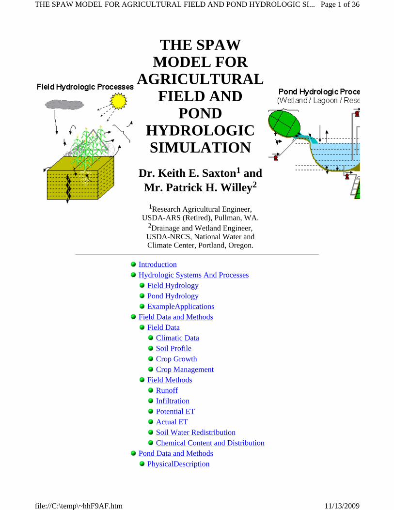
Introduction The SPAW (Soil-Plant-Air-Water) computer model simulates the daily hydrologic water budgets of agricultural landscapes by two connected routines, one for farm fields and a second for impoundments such as wetland ponds, lagoons or reservoirs. Climate, soil and vegetation data files for field and pond projects are selected from those prepared and stored with a system of interactive screens. Various combinations of the data files readily represent multiple landscape and ponding variations.

Field hydrology is represented by: 1.) daily climatic descriptions of rainfall, temperature and evaporation; 2.) a soil profile of interacting layers each with unique water holding characteristics; 3.) annual crop growth with management options for rotations, irrigation and fertilization. The simulation estimates a daily vertical, one-dimensional water budget depth of all major hydrologic processes such as runoff, infiltration, evapotranspiration, soil water profiles and percolation. Water volumes are estimated by budget depths times the associated field area.

Pond hydrology simulations provide water budgets by multiple input and depletion processes for impoundments which have agricultural fields or operations as their water source. Data input and selection of previously defined data files are by graphical screens with both tabular and graphical results.Typical applications include analyses of wetland inundation duration and frequency, wastewater storage designs, and reliability of water supply reservoirs.

The objective of the SPAW model was to understand and predict agricultural hydrology and its interactions with soils and crop production without undue burden of computation time or input details. This required continual vigilance of the many choices required for the representation of each physical, chemical and biological process to achieve a "reasonable" and "balanced" approximation of the real world with numerical solutions.

Over the development period, both the model and the method of data input with system descriptors have evolved for improved accuracy, extended applications, and ease of use. The program documentation includes theory, data requirements, example applications, and operational details. The model results have been corroborated through research data, workshops and application evaluations.

Sinks and SourcesSimulations and ResultsCalibration and SensitivityCorroboration of ResultsExample Water Budgets

Dryland CroppingIrrigated CroppingWastewater Storage PondWetland Hydrology

Options and EnhancementsCurrent Model StatusInstallation and AvailabilitySummary



The SPAW-Field model is a daily vertical water budget of an agricultural field, provided the field can be considered, for practical purposes, spatially uniform in soil, crop and climate. These considerations will limit the definition of a "field" depending on the local conditions and the intended simulation accuracy. For many typical cases, the simulation will represent a typical farm field of tens to a few hundred acres growing a single crop with insignificant variations of soil water characteristics or field management. In other cases, a single farm field may need to be divided into separate simulation regions because of distinct and significant differences of soil or crop characteristics. These definitions and divisions will depend on the accuracy required, however users soon gain enough experience through alternative solutions to guide these choices.

Since the field model has no infiltration time distribution less than daily and no flow routing, it is generally not applicable for large watershed hydrologic analyses. However, it can be utilized for water budgets of agricultural watersheds composed of multiple farm fields, each simulated separately and the results combined. The combined field concept to represent a watershed is used as an input source for the pond simulations. With no streamflow routing there are no channel descriptors included. Daily runoff is estimated as an equivalent depth over the simulation field by the USDA/SCS Curve Number method.

The SPAW-Pond model simulates the water budget of an inundated depression or constructed impoundment. The water supply to the inundated area is estimated runoff from one or more previously simulated fields, plus, if applicable, that from external sources such as an off-site pump or flush water from an animal housing facility. Pond climatic data are provided from that input to the field simulation. Additional features are included such as outlet pipe discharge, drawdown pumps, irrigation supply demands and water tables to allow for a wide variety of pond situations described as wetlands, small ponds, water supply reservoirs, lagoons or seasonal waterfowl ponds.

Basic interactions of soil chemicals such as nitrogen and salinity with soil water and crop production are included. The chemistry is represented in daily budget form, thus does not include interactions and minor processes which occur within soil and crop environments. These budgets are useful as a screening tool to define potential effects and hazards related to the chemical inputs and dispositions for situations often encountered in agricultural hydrologic analyses.

Hydrologic Systems And Processes | Field Data and Methods | Pond Data and Methods | Simulations and Results | Calibration and Sensitivity | Corroboration of Results | Example Water Budgets | Options

and Enhancements | Current Model Status | Installation and Availability | Summary

Hydrologic Systems and Processes Simulating the hydrologic budget of an agricultural field or pond requires defining the hydrologic system and associated processes. The field budget utilizes a one-dimensional vertical system beginning above the plant canopy and proceeding downward through the soil profile a depth sufficient to represent the complete root penetration and subsurface hydrologic processes (lateral soil water flow is not simulated). The pond hydrologic system is an impoundment with external inputs from a watershed or supplemental water sources and outflow by spillways, pumps and seepage. The following schematics illustrate the field and pond hydrologic systems and major processes.

Field Hydrology | Pond Hydrology | ExampleApplications



Introduction | Field Data and Methods | Pond Data and Methods | Simulations and Results | Calibration and Sensitivity | Corroboration of Results | Example Water Budgets | Options and Enhancements |

Current Model Status | Installation and Availability | Summary

Field Hydrology The principle hydrologic processes in the SPAW-Field model are depicted in Figure 1 by a schematic of the vertical budget of an agricultural field:

Precipitation: Daily observed totals, although snow accumulation and snowmelt are estimated when air temperature is included. Applied irrigation water is a supplement without runoff.

Runoff: Computed by the USDA/SCS Curve Number method as a percent of daily rainfall from parameters of soil type, antecedent soil moisture, vegetation, surface conditions and frozen soil. No stream routing is provided. Observed runoff can be substituted or compared to simulated values.

Infiltration: A daily amount based on rainfall minus estimated runoff and stored in the uppermost soil layers as available capacity permits.

Evapotranspiration: Combined daily estimates of plant transpiration, direct soil surface evaporation and interception evaporation estimated from a daily atmospheric potential evaporation reduced by the plant and soil water status. The potential evaporation input data may be estimated by one of several methodssuch as the Penman and/or Monteith equation, daily pan evaporation, temperature or radiation methods, or mean annual evaporation distributed by months and monthly mean daily.

Redistribution within the soil profile: Infiltrated water is moved between soil layers by a Darcy tension-conductivity method to provide both downward and upward flow estimates. Soil water holding characteristics of tension and conductivity are estimated from soil textures and organic matter and adjusted for density, gravel and salinity. Observed soil moisture can be substituted or compared to simulated values.

Percolation: Water leaving the bottom layer of the described soil profile. Percolated water is considered to be temporarily stored in an "image" layer just below the profile and is upward retrievable. Upward percolation (negative) is considered for cases of groundwater occurrence.

Deep drainage: Deep drainage to groundwater or interflow occurs when the image layer achieves near saturation and additional percolation occurs.

Chemical applications and redistributions: Nitrogen and salinity chemicals are budgeted with plant uptake and soil water transport interactions to estimate soil layer quantities, soil water concentrations and percolation.

Hydrologic Systems and Processes | Pond Hydrologic Processes | ExampleApplications Introduction | Field Data and Methods | Pond Data and Methods | Simulations and Results | Calibration

and Sensitivity | Corroboration of Results | Example Water Budgets | Options and Enhancements | Current Model Status | Installation and Availability | Summary



Pond Hydrology The principle hydrologic processes considered in the SPAW-Pond model are depicted in Figure 2 by a schematic of the inflows, withdrawals and losses. A depth-area table describes the ponded area plus specific depths above the pond bottom for permanent storage, pump inlets, pipe-outlet and the emergency spillway outlet. Each of these depths provides operational limits of the various budgeting processes such as the pumps, pipe outlet, or irrigation water.

Watershed inflow: Daily water supplied to the pond by watershed runoff comprised of one or more fields that have had runoff estimated by a SPAW-Field simulation.

Subsurface inflow: Daily water supplied to the pond by a percentage of the estimated watershed field deep drainage.

Pond inflow: Outflows from an upstream pond estimated by a prior pond simulation.

Side Slope Runoff: Runoff from pond side-slopes above the current water level.

External input: Water supplied to the pond from a source other than a watershed such as an off-stream pump or an animal housing flush system. An optional pump control by specified upper and lower pond depth limits provides hydrologic-based decisions.

Rainfall: That precipitation falling directly on the pond water surface.

Evaporation: Daily water surface evaporation estimated as the potential of the climatic data.

Infiltration: An infiltrated water depth into the pond bottom soil as it is initially inundated.

Seepage: A constant daily seepage rate beneath the inundated area (positive), or upward groundwater seepage into the pond due to external high water levels (negative).

Outlet Pipe: Daily discharge of a pipe outlet having a specified crest elevation above the pond bottom and a stage-discharge relationship for depths above the crest. Crest heights may be varied over time for seasonal water depth management.

Spillway overflow: An unregulated daily discharge from the uppermost spillway or outlet when inflow exceeds pond storage.

Supply pump: A daily amount pumped from the pond for designated periods and rates with a specified inlet depth for various water supply needs.

Drawdown pump: A daily amount withdrawn from the pond for designated periods and rates for storage management with a specified inlet depth. An optional pump control by specified upper and lower pond depth limits provides hydrologic-based decisions.

Irrigation demand: A daily irrigation amount supplied by the pond to one or more fields previously defined by a SPAW-Field water budget simulation with irrigation for each field if pond water is above a specified inlet depth.



Water Table: A time varying water table depth external to the pond such as a nearby waterway or river which may supply water to the pond each year by negative seepage.

Permanent Pool: Depths between the lowest outlet pipe or structure intake and the pond bottom.

Active Pool: Depths between lowest pipe or structure intake and pipe outlet crest elevation.

Flood Pool: Depths between pipe outlet crest elevation and spillway elevation.

Hydrologic Systems and Processes | Field Hydrology | ExampleApplications Introduction | Field Data and Methods | Pond Data and Methods | Simulations and Results |

Calibration and Sensitivity | Corroboration of Results | Example Water Budgets | Options and Enhancements | Current Model Status | Installation and Availability | Summary

Example Applications The SPAW water budget model can be adapted to a wide variety of hydrologic analyses within the constraints of the programmed processes and data available. Some example applications for agricultural fields and ponds would be:

Evaluating the daily status of available crop water under rainfall or irrigation regimes. Estimating runoff and seepage from agricultural fields. Scheduling irrigation or defining irrigation requirements. Assessing deep seepage of field water and chemicals which may contribute to water and nutrient losses. Defining depths, frequency and durations of agricultural wetland inundations. Design and performance evaluation of agricultural ponds, lagoons and reservoirs for water supply, waste management and water management. Estimating soil nitrogen or salinity budgets and concentrations for crop production and salinity hazard.

Hydrologic Systems and Processes | Field Hydrology | Pond Hydrology Introduction | Field Data and Methods | Pond Data and Methods | Simulations and Results |

Calibration and Sensitivity | Corroboration of Results | Example Water Budgets | Options and Enhancements | Current Model Status | Installation and Availability | Summary

Field Data and Methods Each major hydrologic process in the field and pond environment is simulated individually, then combined to develop daily water budgets for the system components. Each process requires specific descriptions of the physical parameters and influencing variables followed by appropriate fixed and dynamic data inputs. This approach is similar to that first outlined by Saxton et al., 1974a, 1974b and similar to that of other models (Feddes et al., 1980; Malone et al., 2001). The following summarizes the major hydrologic input data and processes.



Introduction | Hydrologic Systems And Processes | Pond Data and Methods | Simulations and Results | Calibration and Sensitivity | Corroboration of Results | Example Water Budgets | Options


Field Data Field input data are in three general categories of climate, soils and crops. The climatic data are those from a climatic data base and regional estimates. Soils data are interpretations from soil profile descriptions of those typical of the simulated field. Crop data are annual descriptions of locally observed crop growth parameters. The crop data are supplemented by management options such as rotations, irrigation and nitrogen fertilizer chemicals.

The data input files are recorded and assembled via a series of data input screens with the exception of observed climatic data files which are manually copied to a directory. Each screen saves a unique data file in the computer directory such as daily climate, soil profiles and individual crop growth parameters which then become selectable for subsequent simulations. These saved data files provide the user an opportunity to describe data unique to the study region for individual crops, soils and climates. These files may be accessed in later simulations in various combinations as fields and pond descriptions require, thus minimizing input duplication. New files can be created by copying and modifying existing files.

Field Data and Methods | Field Methods Introduction | Hydrologic Systems And Processes | Field Data and Methods | Pond Data and Methods | Simulations and Results | Calibration and Sensitivity | Corroboration of Results |

Example Water Budgets | Options and Enhancements | Current Model Status | Installation and Availability | Summary

Climatic Data Field water budgets are significantly dependent on the climatic inputs of precipitation and potential evaporation which control water input and evapotranspiration, ET, the largest depletion process. Climatic data are input in three categories: 1) historic measured climatic data for the local region, 2) default daily potential evaporation values by monthly estimates, and 3) selected data pertinent to a specific location. The historic climatic data files are copied into a SPAW directory from external sources while the default and location files are created by input screens.

Climatic files of measured data can be obtained in text form from usual sources such as NOAA National Climatic Data Center or the USDA/NRCS Water and Climate Center. Other techniques may be used if necessary (Osborn et al., 1982). These files must contain daily precipitation data. Daily max/min temperatures and potential evaporation are optional. The required data file header and format are specified in the program HELP menu. Daily precipitation generally dominates the accuracy of field water budgets, thus it is imperative that these data be correct and appropriate to the field location. A screening tool is provided to review and edit the climatic data for unusual and



missing values.

Snow accumulation and melt become important in cold climates by delaying the infiltration of precipitation. Most climatic data files do not distinguish the form of precipitation being either rain or snow, thus air temperature data are used to estimate snow accumulation and melt to provide an approximate daily distribution of available water to the infiltration process. Calibration parameters are included to adjust for local variations. Snow accumulation occurs for any day which has precipitation and the mean daily temperature and the previous 5-day average temperature are at or less than 32 oF.

A daily estimate for PET is required for simulation each day, either from observed or estimated data. Daily measurements or estimates are input by copying to the climatic data file. It is often the case that daily PET data are incomplete or not available. To meet the need for a daily estimate for periods of missing data, a default data set of mean monthly daily values is input with monthly adjustment coefficients appropriate to the estimating method and region. A common approach is to apportion apply annual pan evaporation to each month and include a monthly pan-to-PET coefficient. Estimating mean monthly daily values by an energy based method such as Penman-Monteith or regional "lake" evaporation would allow coefficient values near 1.0 (Farnsworth et al., 1982; Saxton and McGuinness, 1982; Jensen et al., 1990)

For a specific field analyses, the applicable location climatic and default PET files previously defined are selected and adjusted if necessary. The model will use daily PET values from the climatic data file if available, but if some, or perhaps all, daily values of PET are not available, monthly mean daily values will be substituted from the default PET file as needed to provide a complete array of daily values for each simulation period.

Field Data | Soil Profile | Crop Growth | Crop Management Introduction | Hydrologic Systems And Processes | Field Data and Methods | Pond Data and Methods | Simulations and Results | Calibration and Sensitivity | Corroboration of Results |


Soil Profile The soil profile is described by incremented layers and water characteristic curves for each layer. Except for the upper and lower boundary, the layers should reflect the soil profile changes plus provide an incremented soil water profile to allow appropriate calculations and definitions. Usually, smaller increments (4 to 8 inches) are used in the first 2 or 3 feet below the surface, then 12 to 18-inch increments thereafter. Thinner layers are not warranted and cause excessive computations while large layers provide excessively broad averages.

The upper and lower boundary conditions for the one dimensional Darcy flow equation have been added to the segmented soil profile as "evaporative" and "image" layers respectively. A set of operational rules are provided for each of these layers. While somewhat arbitrary, they provide useful values to the overall water budgeting processes and are linked with the downward and upward Darcy conductivity estimates.



The upper boundary (evaporative) layer is considered to be a very thin layer (1.0 inch) which rapidly dries with no resistance as in stage-1 soil water evaporation. It re-wets to near saturation by precipitation and dries to a percentage near air dry.

The lower boundary (image) layer is specified below the last soil layer with water characteristics the same as the last layer and a specified thickness. This layer controls deep percolation or upward-flowing water back to the profile. When the water content of the image layer exceeds a specified percentage of its field capacity, water is cascaded downward to become groundwater recharge and is lost from the control volume. If the last real layer becomes drier than the image layer, water is conducted upward from the image layer into the profile, thus it serves as a temporary profile water storage.

Soil water tension and conductivity relationships with moisture are used to define the water capacity and redistribution of each layer. Since these data are often difficult to acquire without laboratory analyses, an estimating routine is included based on soil texture and organic matter, with adjustments for density, gravel and salinity. This texture based method is described in the section on soil water redistribution and is included within the model as a stand-alone module.

Field Data | Climatic Data | Crop Growth | Crop Management Introduction | Hydrologic Systems And Processes | Field Data and Methods | Pond Data and Methods | Simulations and Results | Calibration and Sensitivity | Corroboration of Results |


Crop Growth Plant growth is a very important contributor to hydrologic budgeting through the evapotranspiration effects. Rather than include a plant growth routine to estimate the annual growth characteristics from plant and environment parameters, we chose to provide manual descriptions for the plant growth based on local knowledge of average growth descriptions for major crops Wild, 1988). This approach has proven easy to apply, and sufficient to achieve expected hydrologic accuracies.

The annual crop growth is described by three annual distributions of plant canopy, greenness, and rooting depth. A fourth curve, yield susceptibility, defines the relative impact of annual crop water stress on grain yields when correlated with observed grain yields. For simulations involving nitrogen budgets, the annual nitrogen uptake distribution is included in the crop definitions. Crops growing over the end of the calendar year require two years of definitions. Multiple year crop rotations are developed by selecting the cropping sequence in the "management" screen.

It is useful to see all of the crop descriptive graphs on the same time axes to assure they correspond at selected dates such as planting and harvest. The input screen provides this graph as shown for the corn example in Figure 3.



Percent crop canopy cover represents that portion of the daily potential ET effectively impinging on the plant and not on the soil. It is essentially the percentage of average daily soil surface effectively protected from solar radiation. An annual distribution is described by date-percentage data points throughout the calendar year for daily linear interpolation. The full simulation period must be included for periods less than a full year, and the complete calendar year must be described for multiple year simulations. Residue, green crop or some combination are included in the canopy percentage.

Canopy values can be derived by measurements or visual estimates of soil shading. The model is not highly sensitive to these values, and seasonal distributions of even fast-growing crops provide reasonable results. Measured leaf area index (LAI) is a common measured descriptor which can readily be related to canopy cover by a relationship which shows near full canopy for an LAI value of about 3.0.

A percentage of the described canopy which is green and will readily transpire is entered as Date-Percentage data points. A newly emerging plant canopy over a bare soil would have a Greenness of 100%. A canopy of residue would have a Greenness of 0% unless it had some green weed growth interspersed. As canopies mature or decline due to disease or water stress, they no longer freely transpire, even if soil water is available. These conditions are represented by a declining "greenness" percentage even though the canopy may maintain its stature. The canopy times greenness value approximates the more familiar "crop coefficient" used in many evaporative calculations.

An actively growing canopy generally has an effective rooting system whose maximum depth

Figure 3: Example corn (maize) crop description curves for a calendar year.

Page 10 of 36THE SPAW MODEL FOR AGRICULTURAL FIELD AND POND HYDROLOGIC ...


moves downward at about the same rate as the top growth (canopy) increases. The maximum root depth throughout the calendar year is described as Date-Depth data points. The rooting density and effectiveness for water uptake is partitioned for each 25% of the maximum depth by the 40-30-20-10 percentage as the maximum depths are interpolated between the input data points. Whilerelatively simple, additional detail about root descriptions is generally difficult to measure or describe (Wild, 1988).

The maximum rooting depths and seasonal patterns are quite subject to plant and soil profile characteristics, and local knowledge is often the best guide for hydrologic simulations. Significant year-to-year rooting variations may occur due to water tables, rainfall patterns, etc., and these can be represented if adequate data are available. However, these data would not be applicable to multi-year simulations.

Field Data | Climatic Data | Soil Profile | Crop Management Introduction | Hydrologic Systems And Processes | Field Data and Methods | Pond Data and Methods | Simulations and Results | Calibration and Sensitivity | Corroboration of Results |


Crop Management Management of typical agricultural crops affecting water budgeting most often involve crop rotations. Irrigation and fertilizer application may be options. The management screen provides these parameters for a specific field.

Crop rotations for a field are selected to be in a fixed rotation listed in an annual order and selected from the crop files previously defined. Crop growth characteristics for each selected crop will have been previously described and filed by the crop input screen. Multi-year simulations require each crop to be described for the complete calendar year. Crop rotations are cycled in the order selected and repeated as needed to complete the full simulation period.

Daily irrigation water is budgeted very similar to precipitation. The inputs are either of known irrigation amounts and dates or criteria are provided for the model to determine the time and amount of irrigation water. The irrigation options include ten methods to determine when to irrigate and six to determine how much water to apply as described in Table 1 (Field et al., 1988).

Table 1: Irrigation time and depth options. Time Options for irrigation:

1. Fixed interval: Irrigation occurs on an established initial date and at the user-defined interval in days thereafter.

2. Fixed dates: Irrigation occurs on user-defined dates. 3. Root zone depletion: Irrigation occurs when the soil moisture within the root zone exceeds a

user-defined depletion. 4. Soil profile depletion: Irrigation occurs when the soil moisture within the total soil profile is

depleted below a user-defined limit. 5. Soil water tension at a specified depth: Irrigation occurs when calculated soil moisture

tension in a selected layer exceeds a user-defined value.



6. Soil water tension in root zone: Irrigation occurs when calculated soil moisture tension weighted by root distribution exceeds a user-defined value.

7. Accumulated PET: Irrigation occurs when the calculated accumulation of potential evapotranspiration since the previous irrigation exceeds a user-defined value.

8. Accumulated AET: Irrigation occurs when the calculated accumulation of actual evapotranspiration since the previous irrigation exceeds a user-defined value.

9. Vegetative stress index (moving average): Irrigation occurs when the moving average of the daily vegetative stress index exceeds a user-defined value.

10. Yield reduction index (moving average): Irrigation occurs when the moving average of the daily yield reduction index exceeds a user-defined value. Depth Options for Irrigation:

1. Fixed depth: A fixed depth of water applied at each irrigation. 2. Specified depths: A user-defined depth of water applied for each irrigation. 3. Refill the root zone: A water depth to set the simulated soil moisture level in the root zone

to a user-defined percent of field capacity. 4. Refill the total soil profile: A water depth to set the simulated soil moisture level in the total

profile to a user-defined percentage of field capacity. 5. Accumulated PET: A water depth of a user-defined percent of the potential

evapotranspiration accumulated since the previous irrigation. 6. Accumulated AET: A water depth of a user-defined percent of the actual evapotranspiration

accumulated since the previous irrigation.

Fertilization is an important part of modern crop production and often poses questions related to water management. Daily nitrogen budgeting is included as an option. While not a fully rigorous treatment of chemical budgeting, methods are included to provide nitrogen and salinity budgets within the soil-plant system and interactions with the simulated water budget and transport. The methods are similar to those described by Saxton et al. (1977, 1992b), Burwell et al. (1976), and Malone et al. (2001).

Fertilizer applications for each of the crops in the rotation are listed by date of application, amount and type. The chemical budgets are for nitrogen fertilizers of nitrate or ammonia form. Release of NO3 nitrogen from decaying organic matter and residues is estimated. The salinity budgets provide estimated chemical quantities, profile distributions and leaching. This method focuses on water interactions and does not include chemical-soil solute exchanges.

Observed data

It is often useful to include initial or measured data for the simulated variables such as runoff, soil water, or one of the chemical species. These optional input data by soil profile layers include: soil water, runoff, salinity, nitrate-N, ammonium-N, and negative ion chemical tracer (like nitrate without plant uptake, eg. Cl, Br). The simulation output includes these data used as either a comparison with simulated values or to reset the simulation to be equal to the input data such as for initialization. Standard tabled curve numbers for daily runoff estimates are shown based on theselected soil and crop parameters, or an alternative set of curve numbers can be manually entered.

Field Data | Climatic Data | Soil Profile | Crop Growth Introduction | Hydrologic Systems And Processes | Field Data and Methods | Pond Data and Methods | Simulations and Results | Calibration and Sensitivity | Corroboration of Results |

Example Water Budgets | Options and Enhancements | Current Model Status | Installation and



Availability | Summary

Field Methods The major hydrologic processes within the vertical field water budget are represented by interconnected routines, rates and volumes. The following summarizes those processes most influential in the daily budgets. Detailed equations and variables are generally not included here, but the model contains several additional detailed HELP documents which provide more detail and references.

Runoff | Infiltration | Potential ET | Actual ET | Soil Water Redistribution Introduction | Hydrologic Systems And Processes | Field Data and Methods | Pond Data and Methods | Simulations and Results | Calibration and Sensitivity | Corroboration of Results |


Runoff The USDA/SCS Runoff Curve Number (SCS-CN) method is used to estimate the percentage of precipitation which becomes runoff, or conversely that which infiltrates. Average curve numbers are determined by the model from tabulated values of the SCS-CN method (Rawls et al., 1992; Heggen, 1996; USDA-NRCS, 1997) using entries of land use, treatment, hydrologic conditions (crop condition) and hydrologic soil class. The applied curve numbers for a field can be manually modified by entering values in the Field simulation screen, thus providing an option to calibrate runoff and infiltration volumes. With only daily precipitation and infiltration estimates, there is no sub-daily time distribution of runoff for short-term hydrographs or stream routing.

The published average annual crop curve numbers are modified daily in the model by annual crop canopy and antecedent moisture. The canopy adjustment varies the crop curve numbers upward to equal fallow conditions for no canopy downward an equal amount for full crop cover. Antecedent moisture adjustments for wet and dry conditions (conditions I and III, compared to average wetness, condition II) are estimated from the simulated soil water in the upper soil (layer no. 2). If the moisture of layer 2 is below 60% of field capacity, antecedent condition I is applied; if the moisture of layer 2 is above field capacity, antecedent condition III is applied. No user option is provided for these limits.

Soil freezing significantly restricts infiltration for increased runoff (Fox, 1992). Freezing depths are estimated by air temperature data using methods similar to those reported by Jumikis (1966, 1997). Runoff during frozen soil periods is estimated as 90% of available precipitation, assuming some minor infiltration may yet occur.

Field Methods | Infiltration | Potential ET | Actual ET | Soil Water Redistribution Introduction | Hydrologic Systems And Processes | Field Data and Methods | Pond Data and



Methods | Simulations and Results | Calibration and Sensitivity | Corroboration of Results | Example Water Budgets | Options and Enhancements | Current Model Status | Installation and


Infiltration Daily infiltration is estimated as precipitation minus runoff, with runoff estimated either by the SCS-CN routine, or by observed runoff values if provided. While the estimated infiltration is not given a time distribution less then daily, it is computationally divided into sub-daily time steps used for the water profile redistribution and cascaded to successive deeper layers until adequate storage is achieved. All further redistribution is by the Darcian soil moisture redistribution routine. Should the entire profile reach 90 % saturation due to exceptional rains or restrictive soil layers, additional runoff is estimated.

Field Methods | Runoff | Potential ET | Actual ET | Soil Water Redistribution Introduction | Hydrologic Systems And Processes | Field Data and Methods | Pond Data and Methods | Simulations and Results | Calibration and Sensitivity | Corroboration of Results |


Potential ET The concept and definition of potential evapotranspiration (PET) is not universal among hydrologists and other scientists. However, most agree that the maximum, or potential, largely depends upon the energy available for the liquid-to-vapor phase change, and that this energy source is primarily solar radiation. PET for irrigation-related estimates are often defined as that water lost from a well-watered reference crop such as grass or alfalfa. However practical, this partially confounds the values with some plant and surface characteristics. Methods based on radiation or radiation plus air properties have been the most widely used for short-term estimates such as Penman or Jensen-Haise (Saxton, 1971; Shuttleworth, 1992) These are largely defined by atmospheric variables with minimal surface influence.

Pan evaporation is an indirect, standardized, method of estimating PET with appropriate coefficients. It is generally available for most regions either as daily measurements or monthly and annual means. Large body lake evaporation is a similar approach with minimal coefficient requirements. PET for the SPAW model may be externally obtained from any one of the several meteorological methods with appropriate coefficients.

Field Methods | Runoff | Infiltration | Actual ET | Soil Water Redistribution Introduction | Hydrologic Systems And Processes | Field Data and Methods | Pond Data and Methods | Simulations and Results | Calibration and Sensitivity | Corroboration of Results |




Actual ET The vapor transport of water back into the atmosphere by actual evapotranspiration (AET) is estimated by beginning with daily atmospheric potential ET (PET), then estimating and combining the major AET components: interception evaporation, soil water evaporation and plant transpiration. This approach assumes that the PET is primarily an atmospheric determined value which provides evaporative energy, either radiated or conducted, to a partially wetted surface. The challenge is to evaluate the opportunity of this energy to interact with the various surfaces depending on their current status of wetness and resistance of water to their surface. Energy not utilized in the process of evaporation is available for other uses, largely heating of the near-surface air mass.

Figure 4 provides the computation schematic for the daily estimate of AET obtained by the summation of its components (Saxton et al., 1974a, 1974b). AET is then subtracted from the corresponding source and soil layers. Interception evaporation is removed from the interception storage, soil water evaporation from the first and/or second soil layer (first layer is the thin evaporation layer, second layer can absorb from lower layers), and transpiration from the appropriate soil layers containing roots and moisture.



Interception water is free water on plant and soil surfaces which readily evaporates with minimal surface interaction or vapor resistance. Therefore, the PET value is reduced by the amount of interception evaporation before plant and soil water evaporation are computed. Interception is specified as a storage depth with a constant maximum capacity which represents a potential interception. This storage is filled by precipitation and sprinkler irrigation, and depleted by PET. Defining a potential interception is not obvious. Few data are available and the concept is somewhat nebulous. Each plant canopy has some ability to intercept water and prevent that portion of the precipitation from becoming infiltration or runoff. Surface residues and the uppermost soil surface similarly will wet and dry (not to be confused with depressional storage or soil water evaporation).

Limited data suggests that 0.10 inch is a nominal interception amount for mature agricultural

Figure 4: Computation schematic for estimating actual ET before soil moisture withdrawal and

soil water redistribution.



crops (Shuttleworth, 1992). Plant interception varies over the crop year with the canopy cover percentage. Soil surfaces without the waxy surfaces of most leaves would likely have half this amount. Interception can accumulate to become a significant proportion of the water budget since thirty or forty precipitation events are common in many agricultural climates, which then results in some 3.0 to 5.0 inches of interception evaporation as one component of perhaps 25 to 30 inches of annual AET.

The rate and quantity of evaporation from the upper soil layers is a complicated process of drying and upward water conductivity affected by soil characteristics, tillage, and environmental interactions. Energy and water availability largely dominate the process. This evaporation is not to be confused with that considered as intercepted soil surface water or that in depressional storage which is most often infiltrated.

Soil water evaporation is represented by defining a thin (1.0 inch) upper boundary layer (evaporation layer) of the soil profile. This upper boundary layer has all of the same functions as other layers (except no roots), plus the water is readily evaporated and limited only by that portion of the PET not intercepted by an overlying plant canopy. The lower limit of soil water content in the evaporative layer is approximately air dry.

Upward water movement from the second layer into the evaporation boundary layer and its evaporation is estimated by a modified Darcy equation using a reduced unsaturated conductivity rate for the current soil water content. The reduced conductivity is a small percentage (~5%) of the liquid estimate and represents the fact that the conductivity is largely vapor flow rather than liquid. This method approximates the traditional observed three-stage drying process. Soil surface evaporation can accumulate to several inches over a year depending on the crop canopy, precipitation distribution and PET.

For dry soil conditions with a partial canopy, there is some portion of the radiation energy (PET) which impinges on the soil surface that is not utilized in water evaporation which heats the soil, air, and canopy. It is assumed that a part of this unused soil surface energy is "re-captured" by the partial canopy as added potential transpiration, A canopy value of 60% is set at full capture.

Well-watered, vigorous crops will transpire at nearly the rate demanded by the atmospheric conditions (PET), but as their water supply becomes limited, physical and biological controls begin to limit the rate of transpiration. It is apparent that plant transpiration is a function of both atmospheric evaporative demand and plant available soil water. Plants have unique abilities to control water flow rates within their vascular system and through stomatal action. They make soil water available by root extension and by creating competitive water pressure within their membranes to cause gradients and water flow. A simplified approach based on atmospheric demand and plant available water has been programmed.

The curves of Figure 5 provide a relationship between plant available soil water, defined by the range from wilting point to field capacity, and the ratio of actual transpiration to potential transpiration. The general shape of the curves are based on those derived by Denmead and Shaw (1960, 1962) in controlled small lysimeter studies of corn. These curves express the effect that actual plant transpiration will decrease from potential transpiration in a quite non-linear pattern as plant available water is decreased. The curves representing different levels of PET indicate that for a given level of plant available water, the plant will transpire a greater percentage of PET when PET is low than when PET is high. The curves are applied independently to each defined soil layer in proportion to the percent roots present, thus plant transpiration is estimated as the combined effect of PET, root density distribution, and soil water content and distribution.



For well watered agricultural crops, transpiration can be 15-25 in/yr depending on crop characteristics, growth period and atmospheric demand. Crops with water stress often exhibit significantly less transpiration and reduced yields. The distribution of transpiration over the crop year is variable depending on the crop growth and soil water availability.

Plant roots play a very important role in the connection between evaporative demand at the leaf surfaces and plant available soil water. The dynamic root growth of agricultural crops is particularly influential as the roots penetrate new soil mass and water source. Established plants such as perennial grass also continually grow new roots, but in a less dramatic seasonal pattern (Feddes and Rijema, 1972).

A time-varying root effect is represented by estimating the maximum root depth distribution over the crop growing season. The depth-density distribution is proportioned in the traditional 40-30-20-10 percentage for each 25% of maximum depth downward from the soil surface. Root density is proportionally assigned to each soil layer which then becomes the potential for transpiration water uptake.

The simulation of root water abstraction is not highly sensitive to the rooting description partially because of compensation by soil water redistribution. If root uptake is overestimated for a specific layer, that layer becomes dryer than expected; but the redistribution calculation moves water from adjacent moist layers, thus a compensation of processes.

While this models focus is on hydrologic water budgets of agricultural fields, crop plants play a major role in the water budgeting and if impacted by water stress will have reduced growth and yields. It is a logical extension to estimate the magnitude of transpiration-related water stress and its effects on grain yields, with more minor effects on growth and phenology.

Daily plant stress was defined as:

Stress = 1 - (AT /PT)

Figure 5: Actual over potential transpiration as a function of plant available water and daily PET.



where: AT = Actual transpiration PT = Potential transpiration

By defining AT/PT for each soil layer, the total plant stress is obtained as the root-weighted average of all active soil layers. This provides a weighted estimate of daily crop stress based on PET, profile soil water availability and root density distribution.

Accumulative plant stress over the growing season will impact grain yields, however it is well documented that water stress affects grain yields more severely if it occurs during the fruiting period than during the vegetative phase (Denmead and Shaw, 1960). To represent this relative water stress susceptibility in time and among crops, relative susceptibility relationships as shown for corn and soybeans in Figure 6 are used to weight each days stress over the growing season. This susceptibility pattern is described by arbitrary weighting values of 0.00 to 0.50 entered as date-susceptibility values over the calendar year. These data are optional and have no effect on the simulated water budgets. They are only used for analyses of water stress impacts on grain yields.

Corn

Soybeans



The accumulated stress index values only become meaningful when correlated with observed crop grain yields. Examples such as those of Figure 7 indicate that these correlations can subsequently provide a reasonable estimate of crop water stress effects on yield. A similar approach was successfully applied by Cordery and Graham (1989). There is similar evidence that vegetative growth is closely allied with plant transpiration (Dewit, 1958), thus, the estimated accumulative plant transpiration may also correlate with water stress effects on vegetative crop yields such as forage and grassland. While the water stress is only an index, correlation with yields documents its influence.

Field Methods | Runoff | Infiltration | Potential ET | Soil Water Redistribution Introduction | Hydrologic Systems And Processes | Field Data and Methods | Pond Data and

Figure 6: Example yield susceptibility curves for corn and soybeans (Sudar et al., 1981).

Figure 7: Correlations of computed annual crop water stress index with grain yields in rainfed

fields. (Sudar et al., 1981; Saxton et al., 1992b).



Methods | Simulations and Results | Calibration and Sensitivity | Corroboration of Results | Example Water Budgets | Options and Enhancements | Current Model Status | Installation and


Soil Water Redistribution Soil water is continuously moving in response to pressure gradients caused by capillary and gravimetric forces unique to each soil element according to its pore structure, water content, chemicals, and other minor effects. This water redistribution within the soil profile plays a significant role in the water profile development, up or down percolation and plant water abstraction. It is a very necessary process to be computed for realistic simulations of AET and soil water, although one of the more difficult processes to represent because of the data requirements and mathematical solutions.

A simplified finite difference form of the Darcy equation for vertical water flow up or down between the specified soil layers has been included. The Darcy equation may be expressed as:

q=k(Θ) {[h(Θ)+Z]/Z} (t)

where: q = estimated water flow per time step across layer boundaries, cm k(Θ) = mean unsaturated hydraulic conductivity of the two layers being considered as a function of their respective water contents, cm/hr h(Θ) = matric potential head difference between the two layers being considered as a function of their respective water contents, cm Z = distance between the layer midpoints, cm t = time, hrs Θ = water content, cm3/cm3

While many solutions are available for the Darcy equation (or Richards equation) which use sophisticated numerical analysis techniques, a simplified method of forward differencing was programmed. Variable time steps are defined according to a maximum allowed change of soil water tension per time step. The objective was to minimize the computations, yet provide reasonable redistribution estimates and computational stability over long simulation periods and over the full range of soil water content of agricultural soils.

The pressure and conductivity relationships as a function of moisture content are the most difficult to obtain and input into the model for the redistribution solutions. Measured values of these relationships are very seldom available for hydrologic study sites, yet it is important to use curves that approximate the water holding characteristics of the soil layers. There are numerous estimating methods in literature for various curve parameters, but many require at least some field or laboratory data (Hillel, 1998).

An estimating method for soil water holding characteristics has been developed and included. The technique is a set of generalized equations which describe soil tension and conductivity relationships versus moisture content as a function of sand and clay textures and organic matter (Rawls et al., 1982; 1992; 1998; Saxton et al., 1986). A revised set of equations were more



recently derived by correlation of a very large USDA/NRCS data set (1720 A-horizon samples) assembled to provide continuous curve estimates from wilting point (1500 kPa) to saturation (0 kPa) (Saxton and Rawls, 2004). A programmed texture triangle as an input screen as shown in Figure 8 provides ready solutions to the equations and values for the layer definitions of the model soil profile.

The soil water characteristic equations are valid within a range of soil textures approximately 0-60% clay content and 0-95% sand content. Adjustments to the solutions have been added to include the effects of bulk density, gravel and salinity (Tanji, 1990). This methodology is incorporated in the model and is also available as a stand-alone program. Access to the texture triangle screen is by the icon before the sand percentage in the soil screen. The HELP menu of the texture triangle screen provides additional information and references.

Field Methods | Runoff | Infiltration | Potential ET | Actual ET Introduction | Hydrologic Systems And Processes | Field Data and Methods | Pond Data and Methods | Simulations and Results | Calibration and Sensitivity | Corroboration of Results |


Chemical Content and Distribution Overview: The purpose of the nutrient routine is to estimate the daily nitrogen movement and distribution within a soil profile without the need of large numbers of samples and expensive lab analyses. This was accomplished by adding a model subroutine to the SPAW water budget model to

Figure 8: Texture triangle data screen to estimate soil water holding characteristics.



emulate the addition of chemicals to the plant soil system through fertilizer additions and mineralization as well the estimate the quantity of solute that is moved through various processes including plant uptake, infiltration, and soil profile water redistribution.

The nutrient routine estimates the quantity and location in the profile of nitrate and ammonium form of nitrogen. It also follows the movement of highly soluble non-adsorbed tracers which are not taken up though plant activity. Since the nutrient routine is a satellite of the SPAW water budgeting model, it follows the same order in the calculations of the movement of the chemicals starting with the previous days water content and chemical quantities, adjusting the quantity for the days additions and then calculating the quantities moved through the plant uptake, infiltration and redistribution.

Theory: Fertilizer additions are specified in units of pounds per acre of the ion, eg. NO3. Nitrate and a similar form of tracer are considered available for water transport once added to the soil. Since the ammonium form nitrogen bonds to the CEC (exchange) sites in the soil matrix of most soils, it is not available for transport until after it is biologically converted to nitrate form nitrogen. The daily conversion of the ammonium to nitrate is estimated through an exponentially declining rate function with allow a 90 % conversion within 60 days.

Mineralization is considered following the addition and nitrification processes. The routine takes a given annual returned nitrogen fixed in organic residue from previous crops, a value specified in the input, and assumes a 66% efficiency in the conversion of nitrogen in the form of organic matter to ammonium over a one year period. The addition of the ammonium from the conversion is estimated to occur in daily increments with a time based bell shaped distribution from May 1 to September 30 suggesting the temperature driven soil biological actions.

Plant uptake is estimated by a fixed amount of nitrate uptake over a year period based on being proportional to the rate of development of the canopy. The specified annual quantity of nitrate is distributed over the time span of the canopy development by an "uptake" curve input with the crop development curves. The daily plant uptake is subtracted from the soil layers at a quantity proportional to the water uptake of that layer and the nitrogen concentration of that layer, the water uptake already a function of the layer water content and root density of the day being estimated.

Infiltration and Redistribution: Infiltrating water from rainfall is considered to contain a minor amount of nitrogen in the form of nitrate. The concentration is estimated as 0.75 parts per million (ppm) and this quantity placed initially into the top soil layer.

Under unsaturated soil conditions, nitrate and tracer are assumed to move with the bulk flow. The chemical quantity moved is made equal to the amount of water leaving multiplied by the concentration of the chemical in the layer tht the water is coming from. A minor amount is considered to be held by the soil matrix and not available for transport.

For soil moisture conditions significantly greater than field capacity, it has been observed that more water moves through preferential pathways and contains less than the matrix average concentration of nitrate and tracer. To represent the decreased chemical transport during these wet conditions, the quantity transported from the wet layer is multiplied by a value to represent reduced efficiency, the value variable with the degree of saturation of the contributing layer. The



efficiency function is represented by a "relative saturation" function defined as the percentage of water content ranging from field capacity at 0% to 100% at full saturation. The reduction function ranged from a full 100% transport at field capacity to a curvilinear reduced value of 40 % normal chemical transport at a 40% relative saturation greater than field capacity.

Field Methods | Runoff | Infiltration | Potential ET | Actual ET Introduction | Hydrologic Systems And Processes | Field Data and Methods | Pond Data and Methods | Simulations and Results | Calibration and Sensitivity | Corroboration of Results |


Pond Data and Methods Water budgets for various types of impoundments can be simulated by using appropriate descriptors and data. The schematic of figure 2 indicates the various processes and options, not all of which need to be represented in each pond case.

Three types of inundated areas are typical examples. The hydrology of wetland impoundments whose inputs are largely from agricultural landscapes, constructed lagoons for storing runoff and waste from confined animal feedlots and housing, and small ponds or reservoirs used for water storage. Each of these examples requires a set of physical and hydrologic data.

PhysicalDescription | Sinks and Sources Introduction | Hydrologic Systems And Processes | Field Data and Methods | Simulations and

Results | Calibration and Sensitivity | Corroboration of Results | Example Water Budgets | Options and Enhancements | Current Model Status | Installation and Availability | Summary

Physical Description A Pond Project requires describing the physical and hydrologic parameters of the impoundment to be simulated. A series of tabs is provided on the Pond Project input screen for parameters such as depths, depth-area, seepage rate and outlet pipe rating.

An infiltration amount into the dry pond bottom is estimated based on soil characteristics. This water depth must be satisfied before any inundation will occur, thus prevents ponding with small events. A constant seepage rate below the saturated ponded soil is specified based on the soil and geologic setting. The infiltration and seepage areas vary as the impoundment fills or empties. No evapotranspiration is estimated for the fringe area of the wetted perimeter.

The physical size and shape of the impoundment is defined by depth-area values incremented from the pond bottom to above the maximum spillway. Depths are specified with reference to the bottom. These values for natural ponds or wetlands can be estimated from topographic elevation maps while constructed ponds have more uniform and known dimensions.



An outlet pipe may be specified at an elevation less than the uppermost spillway outlet having a crest elevation and a stage-discharge flow rate above that depth. This outlet pipe could be one of many configurations from typical outlet weirs with pipes through the dam fill material, simple outflow drop box control structures and tile drains from wetlands. The crest elevation can be changed over a calendar year to accommodate situations such as variable drop box board changes to create seasonal ponding control.

Pond Data and Methods | Sinks and Sources Introduction | Hydrologic Systems And Processes | Field Data and Methods | Simulations and


Sinks and Sources The pond watershed is represented by selecting one to several previously simulated Field Projects with an associated size and deep drainage (interflow) percentage captured by the pond. Direct precipitation and evaporation of the pond surface are transferred from the last watershed field selected. Runoff from the exposed pond banks is added.

An external water supply is programmable to represent a variety of inputs ranging from an offsite supply pump to wash water from animal housing or product processing. This daily influx is specified for selected periods and rates. The inflow can be program controlled with specified upper and lower depth limits to estimate water inputs required to maintain the set water volumes. Single day amounts are specified as the same date in both the beginning and ending date entries.

Irrigated fields may be considered for water withdrawal with an outlet or pump having a specific inlet depth. The amount and schedule of these withdrawals depends on the irrigated field having been previously simulated with an irrigation schedule option. A field size and irrigation efficiency are specified. Irrigation water is removed from the impoundment if available above the outlet depth, and any lack of required water is documented as an irrigation deficit.

Several pumping options may be selected to remove ponded water. A supply pump will remove water for daily applications such as stock water supply by specifying an inlet depth, operation periods and rates. Any specified pumping not met due to low water levels is documented as a deficit to evaluate the reliability for the intended purpose.

A drawdown pump may be specified for water level control in systems such as wastewater storage lagoons. By defined intake elevation, operational periods and discharge rates, the water is removed to an external site such as an irrigated disposal field. An option of program-determined pond level control can be set such that pumping begins at a set upper level and stops at a lower level. Both manual and automatic pumping options assist with the selection of pump size and operation periods to meet water level requirements.

Water may influx from external ground water such as a nearby seasonal river rise. Groundwater levels relative to the pond bottom determined from an external data source are input to estimate upward seepage into the pond at the specified pond seepage rate until the pond and water table depths are equal. As the ground water levels go below the pond elevation, seepage out of the pond



resumes. The rate of seepage is controlled by the pond seepage rate.

Impoundments may occur in a sequence with those downstream receiving water from those upstream such as sequential settling and storage ponds. These inputs are made with sequential simulations beginning with the one uppermost. A percent of each upstream outflow is specified as inflow to allow for flow losses or divisions.

All daily pond computations are divided into 24 hourly segments, thus no single process is allowed more than an hourly change before readjusting the pond depths and other effected processes. This is particularly important for the Outflow Pipe flow based on a discharge depending on water stage above the Pipe Outlet.

Pond Data and Methods | PhysicalDescription Introduction | Hydrologic Systems And Processes | Field Data and Methods | Simulations and


Simulations and Results Simulations for either a Field or Pond Project begins by selecting either an existing project file or creating a new file from the Project menu. Projects are filed by Location/Field or Location/Pond to provide a readily accessible directory. Each Field project file is completed by selecting previously defined location climate, field management and soil data files appropriate to that field. In addition, any observed data are entered, the runoff curve numbers reviewed or changed, output files selected and simulation dates specified within those of the climatic data.

New or existing Pond Project files are defined from selected tabs of the input screen. Only those options appropriate to the current impoundment need be completed. At least one previously simulated Field must be selected to provide runoff and climatic data. A minimum set of depths and depth-area values are required. The simulation period within the dates of the watershed data and selected output files are specified.

Each field and pond simulation begins with the assimilation of input data from the selected previously defined files and the project input screen. This data file is written and used as the principle input data to the model. It can be reviewed for input assurance, or manually modified and re-run by advanced users using the "Options/Manual Run" menu.

Each Field or Pond simulation generates a set of selected output files available directly after the simulation under the View menu. These can also be re-opened at any later time by again selecting the Project Field or Pond screen. Each field output file is labeled with user information, simulationdates and complete file descriptions followed by labeled variables. Pond output tables provide user information, simulation dates, file information plus the descriptive data of the simulated impoundment.

Budget summaries for time periods of annual, monthly and daily are provided. Average data for each time period (annual, monthly or daily) are shown at the end of each summary table. Each output table is compatible with word processing or spread sheet programs (tab delineated) to be



viewed, edited, printed or analyzed.

For wetland hydrologic analyses, results are a summary of inundation periods, defined as individual periods when separated by one or more days of dry pond. A statistical summary of the inundation periods for the entire simulated period is provided at the end of the report. This shows the percentage of years the inundation periods met the criteria of wetland hydrology by each 10% of the maximum pond depth. Pond summaries also include depth durations as the number of days the pond depths equaled or exceeded the indicated depths in 10% increments of the maximum depth.

An optional detailed field hydrology report contains one of three levels of budgeting output which can be selected for simulation accuracy assurance or error analyses. The "Minimum" level shows only daily totals, "Medium" provides budgets for each soil layer, and "Maximum" provides soil water movement each delta time increment for each soil layer. These "detailed" files should be selected with caution since they can become very large for long simulation periods.

A graph routine is provided to visually view daily hydrologic values within the field and pond budgets. Daily and accumulative values for most variables are selectable. Soil water and chemical values are graphed by total profile, each soil layer or a combined graph of all layers under the label "Stack". The pond graph is similar to that of the field with both daily and accumulative variable values over each calendar year. The time period of the graph is selectable by months (1-24) and years. The graphs can be saved using the "File/Save As" option.

Introduction | Hydrologic Systems And Processes | Field Data and Methods | Pond Data and Methods | Calibration and Sensitivity | Corroboration of Results | Example Water Budgets | Options and Enhancements | Current Model Status | Installation and Availability | Summary

Calibration and Sensitivity Simulation results are achieved by combining the products of several hydrologic processes, each of which has been developed from research results and physical understanding. Thus, calibrating the model consists of identifying the appropriate parameters and coefficients for each of these processes. Each input has a method to estimate values based on experience and data to assure a solution within expected hydrologic accuracy.

For those cases when results need to be altered to better represent measured data or experienced estimates, calibrations can be accomplished by identifying which of the several hydrologic processes will impact the values being evaluated. An overview of the input screens provides a suite of the parameter and data choices which might be altered. Field examples would be the evaporation pan coefficients, runoff curve numbers, soil water holding characteristics, and crop growth descriptors. Pond parameters may also need to be justified such as seepage and dry bottom infiltration.

Precipitation and evaporation data and parameters have the most influence on water balance computations with variations in caused by location, elevation or local anomalies. Adjustment factors are available to modify observed precipitation, temperature and evaporation data. Evaporation coefficients are generally more stable over time and space than other climatic data



and thus easier to effectively define.

Runoff estimates by the curve number method is one of the more empirical process representations. Standard tabled estimates of the curve number values are derived, but these can be replaced by manual estimates. Even after calibration, significant deviations of daily runoff and infiltration from actual values can be expected, but averages over longer periods can generally be adequately calibrated.

The impact of soil and plant descriptors and parameters are generally less sensitive than those climactically related. While both soil and plant impacts are very important, their representation is often easier to document, thus, with less sensitivity, also less likely to require significant calibration for broad scale water budgets. An exception would be those analyses focused on crop production in which both soil water and crop parameters become increasingly important.

Introduction | Hydrologic Systems And Processes | Field Data and Methods | Pond Data and Methods | Simulations and Results | Corroboration of Results | Example Water Budgets | Options


Corroboration Of Results Establishing the utility and accuracy of a hydrologic model varies with the focus of the model and the analytical intent. The SPAW model is most useful for those water budgets involving agricultural soils and crops, thus significant effort has been given to these descriptions and representations. Most analyses using the model would include field runoff, soil water and pond budgets, thus assurances of these estimates becomes important.

Estimating runoff by the USDA/SCS curve number method is based on the long term data sets used in its derivation, thus it is best representative of annual streamflow volumes. The original data sets were from the Great Plains region of central US, thus it best represents summer convective rainfall events. A transect study from Western Kansas to Eastern Missouri (Saxton and Bluhm, 1982) showed reasonably good agreement of the estimated annual runoff for regions with annual precipitation ranging from some 10 to 40 inches.

Of particular importance are the soil water profile dynamics over time. Simulated soil water has been extensively compared with measured data in a wide range of climate, soil and crop combinations. Most of the soil moisture measurements have been by the neutron probe method supplemented by surface samples. Figure 9 shows a comparison of observed and predicted soil water by soil layers with the model initialized the first measurement of each year.



The model has been extensively tested on agricultural crops such as corn, soybeans, brome grass, and wheat (Sudar et. al 1981; DeJong and Zentner, 1985; Saxton, 1985, 1989; Saxton and Bluhm, 1982; Saxton et al. 1974a, 1974b, 1992a, 1992b). Additional applications have shown similar results for other dryland crops such as sorghum and pearl millet (Omer et al., 1988; Rao and Saxton, 1995; Rao et al., 1997). Several studies for irrigated conditions showed good agreement of measured and estimated soil moisture for scheduling and economic analyses (Field et al., 1988; Bernardo et al., 1988a; 1988b).

Some calibration is recommended wherever possible. The calibration technique found most useful is to compare measured and observed soil water. This is not a complete calibration since AET and percolation are not include. Only lysimeter data would provide this complete data set such as that described by Maticic et al., 1992a; 1992b. Time distribution of soil water data usually suggests which model parameters or representations need adjustment. Early experience with the model willgenerally suggest which parameters are changeable for calibration and what processes each will affect.

Estimating soil chemical interactions with water and plant activity has been estimated and compared with measured data (Saxton et al., 1977, 1992a; Burwell et al., 1976). While these have not been extensive studies, their reasonable budgets and concentrations lend credibility to the approach.

Applications of the POND model have ranged from determining wetland inundation frequencies, sizing stock watering ponds for minimal deficiencies, sizing waste water lagoons and associated pumping capacities, and the long-term levels of wildlife ponds (Saxton and Willey, 1999; 2004). With the many operational inputs included in the pond model, simulations can be achieved for many pond types. Similar to the field hydrology, pond hydrology is generally best understood by analyzing pond states and processes over times of days and years. The tabled and graphical outputs provide many analytical opportunities. Recent evaluations of pond budgets for waste water storage pond design was presented by Moffit et al. (2003) and Moffit and Wilson (2004). Figure 10 shows measured and simulated wastewater pond depths over a three year period.

Figure 9: Observed and simulated soil water for three crop years with corn in Western Iowa

(Sudar et al., 1981).



Introduction | Hydrologic Systems And Processes | Field Data and Methods | Pond Data and Methods | Simulations and Results | Calibration and Sensitivity | Example Water Budgets |

Options and Enhancements | Current Model Status | Installation and Availability | Summary

Example Water Budgets Example results by SPAW simulations demonstrate several typical applications of the field and pond water budgets. Only limited graphical results are shown, although each simulation produced the full suite of tabular and graphical results, usually over a multi-year period. The examples showresults for fields of rainfed and irrigated cropping plus wetland and storage ponds.

Example Water Budgets | Dryland Cropping | Irrigated Cropping | Wastewater Storage Pond | Wetland Hydrology

Introduction | Hydrologic Systems And Processes | Field Data and Methods | Pond Data and Methods | Simulations and Results | Calibration and Sensitivity | Corroboration of Results | Options and Enhancements | Current Model Status | Installation and Availability | Summary

Dryland Cropping Soil water in rainfed cropping is subject to the amount and time of precipitation. The example shown in Figure 11 demonstrates the daily variation of soil water distributions by soil layers over a cropping season. Periods of rainfall replenish the profile followed by periods of evapotranspiration depletion. The moisture "stack" shows total soil profile water accumulated by soil layers (thickness times %v) for each day.

Figure 10: Simulated and measured waste water storage pond depths (Moffit and Wilson 2004).



Example Water Budgets | Irrigated Cropping | Wastewater Storage Pond | Wetland Hydrology Introduction | Hydrologic Systems And Processes | Field Data and Methods | Pond Data and Methods | Simulations and Results | Calibration and Sensitivity | Corroboration of Results | Options and Enhancements | Current Model Status | Installation and Availability | Summary

Irrigated Cropping Supplemental crop water by irrigation involves significant expense and time. Irrigation decisions are often based on limited data or judgment information about the plant-soil-climate system. In some cases, water loss and excessive chemical leaching may result. Using water budget results such as the example shown in Figure 12 can assist to optimize water requirements, plant responses and water efficiencies. The simulation was based on irrigation dates "model-determined" at 40% root zone depletion and irrigated depths of two inches.

Figure 11: Daily precipitation and soil water by soil layers for a rainfed corn field in Eastern

South Dakota.



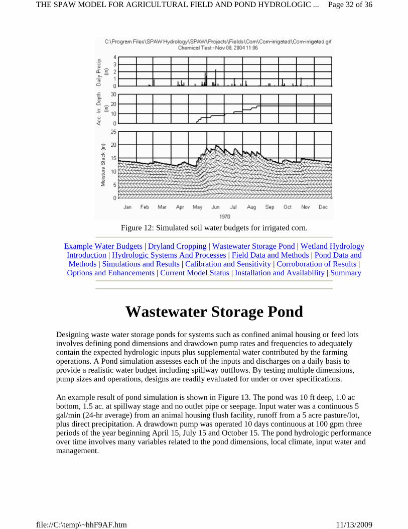
Example Water Budgets | Dryland Cropping | Wastewater Storage Pond | Wetland Hydrology Introduction | Hydrologic Systems And Processes | Field Data and Methods | Pond Data and Methods | Simulations and Results | Calibration and Sensitivity | Corroboration of Results | Options and Enhancements | Current Model Status | Installation and Availability | Summary

Wastewater Storage Pond Designing waste water storage ponds for systems such as confined animal housing or feed lots involves defining pond dimensions and drawdown pump rates and frequencies to adequately contain the expected hydrologic inputs plus supplemental water contributed by the farming operations. A Pond simulation assesses each of the inputs and discharges on a daily basis to provide a realistic water budget including spillway outflows. By testing multiple dimensions, pump sizes and operations, designs are readily evaluated for under or over specifications.

An example result of pond simulation is shown in Figure 13. The pond was 10 ft deep, 1.0 ac bottom, 1.5 ac. at spillway stage and no outlet pipe or seepage. Input water was a continuous 5 gal/min (24-hr average) from an animal housing flush facility, runoff from a 5 acre pasture/lot, plus direct precipitation. A drawdown pump was operated 10 days continuous at 100 gpm three periods of the year beginning April 15, July 15 and October 15. The pond hydrologic performance over time involves many variables related to the pond dimensions, local climate, input water and management.

Figure 12: Simulated soil water budgets for irrigated corn.



Example Water Budgets | Dryland Cropping | Irrigated Cropping | Wetland Hydrology Introduction | Hydrologic Systems And Processes | Field Data and Methods | Pond Data and Methods | Simulations and Results | Calibration and Sensitivity | Corroboration of Results | Options and Enhancements | Current Model Status | Installation and Availability | Summary

Wetland Hydrology An example analysis for a ponded wetland within a corn field in the vicinity of Jonesboro, AR was simulated for 30 continuous years using rainfall data from the USDA/NRCS climate center (AR3734), annual evaporation of 53 inches, a well drained silt loam soil, and continuous corn crop. The wetland pond had a maximum depth of 6.0 ft. before uncontrolled spillage, an area of 1.0 ac at 0.0 depth, and a maximum area of 7.5 ac at the 6.0 ft. depth. A moderately high seepage rate of 1.0 in/day was assumed, and the corn field drainage area was 50 ac.

The subsequent daily inundation simulations provided annual distributions of ponded depths as shown for 1991 in Figure 14. A summary and analyses routine provided wetland statistics according to the inundation criteria of being inundated a specified number of days within the "wetland" growing period of the year for more than 50% of the years. For this example, a ponded depth of approximately 2.4 ft. with an associated area of about 2.0 acres was defined to meet the hydrology component of wetland criteria.

Figure 13: Example daily water budget of a waste water storage pond for an animal housing

facility and adjacent lot with drawdown pump operated three times per year.



Example Water Budgets | Dryland Cropping | Irrigated Cropping | Wastewater Storage Pond Introduction | Hydrologic Systems And Processes | Field Data and Methods | Pond Data and Methods | Simulations and Results | Calibration and Sensitivity | Corroboration of Results | Options and Enhancements | Current Model Status | Installation and Availability | Summary

Options and Enhancements Several features have been incorporated which extend the model capability or provide options for user preferences. Each user completes identifying information, multiple users can use the same program and data files, and each output file identifies the current user. Several choices of units allow corresponding values with those most familiar, for example English or metric units for graphing and the soil water characteristics; gravel percentages by weight or volume.

At the time of installation, several options are available for loading part or all model components and a directory choice, although default values are suggested for unfamiliar users. Choices are available for program display features of file selection and display preferences. The soil water characteristic graph has two scales and unit options.

For advance users, a "manual run" option is available to run an existing "input data" file generated by the Field or Pond Project screens. This is useful if the usual data values need to be manually modified to better represent the desired simulation. Obviously this requires extreme care in format

Figure 14: Daily rainfall, watershed runoff, and inundation depth for a wetland during 1991 near

Jonesboro, AR.



and value selection to avoid invalid data input.

Introduction | Hydrologic Systems And Processes | Field Data and Methods | Pond Data and Methods | Simulations and Results | Calibration and Sensitivity | Corroboration of Results | Example Water Budgets | Current Model Status | Installation and Availability | Summary

Current Model Status This model, like most, was achieved by being developed, modified, supplemented, tested and revised. New versions are developed just as new models of manufactured machines are brought to the market. While the SPAW model has been developed over several years and iterations to achieve a stage of correctness and utility, users would be advised to check the WEB site (http://hydrolab.arsusda.gov/SPAW/Index.htm) or correspond with the authors and supporting agencies before extended new applications.

The field hydrology components have been quite well developed and tested. Some exceptions are the frozen soil predictions and its impact on the infiltration and the snow accumulation and melt routines that have had several "reality" checks but not extensive verification. Additions to the lower soil boundary to represent varying drainage and groundwater possibilities beyond the verified "well drained" case have more recently been added and as a result not as thoroughly tested.

Many pond water budgets have been verified or evaluated by experienced hydrologists. Daily budget components are continually balanced and verified for mathematical correctness. Even so, as with any multiple variable simulation, a possibility always remains for an undetected error or interaction, thus each user must be hydrologically cognizant of their results and implications.

The nitrogen and salinity budgets have not had extensive field verification. While we believe these methods will provide reasonable estimates, they should be used cautiously as a screening tool or verified with observed data. The authors and sponsoring agencies would be very appreciative to be notified of any detected errors or irregularities in any of the modules or applications.

Introduction | Hydrologic Systems And Processes | Field Data and Methods | Pond Data and Methods | Simulations and Results | Calibration and Sensitivity | Corroboration of Results |

Example Water Budgets | Options and Enhancements | Installation and Availability | Summary

Installation and Availability The default model installation places the model and all data files in the disk directory "Program Files/SPAW Hydrology/SPAW". This is a fixed directory format and requires no user knowledge or interference once loaded. The only user interaction generally expected is to copy the climatic data files into the directory "SPAW/Database/Climates/Data". All generated files by either the



data screens or Field and Pond simulations can be found in this directory location.

The model will readily perform on a modern PC computer running Microsoft Windows 95 or newer, 486/Pentium or similar processor, and moderate size hard drive. Memory should be least 256 MB of RAM plus adequate hard disk space for Project results. It is suggested not to simultaneously run additional programs to avoid memory conflicts. A mouse driven screen pointer is most convenient to quickly operate the screens, although keyboard controls are available for most functions. Typical run times for a 30 year simulation on a 1,000 Hz processor are about 1.0 min for the field and 0.5 min for the pond.

General information about the SPAW model and latest versions can be found at the following Web Page: (http://hydrolab.arsusda.gov/SPAW/Index.htm). You will be asked to "register" prior to downloading the program files to provide contact opportunity for up-dates and corrections as needed. The program and example data files are available on CD's by request to the contact personnel.

This program was developed through the support of the US Department of Agriculture agencies of Agricultural Research Service and Natural Resource Conservation Service (formerly Soil Conservation Service) and is publicly available. No written agreement, license, or royalty fee is required for use or distribution, however this software is provided "as-is," without any express or implied warranty or accuracy. User training and support are provided by the agencies to their staff. Additional support can be requested from the authors or their representatives.


Example Water Budgets | Options and Enhancements | Current Model Status | Summary

Summary The agricultural hydrology model, SPAW, consists of two linked routines, a daily vertical water budget of an agricultural field and a daily impoundment water budget. The field model input includes daily climate data, annual crop definitions, and a layered soil profile with individual tension-conductivity soil water characteristics. The ponding routine utilizes the climatic data and runoff estimates from one or more previously simulated farm fields, physical descriptions of depth-area, pipe and pump flow rates and process parameters. The pond simulations may be applied to shallow wetlands, small ponds, or constructed lagoons and reservoirs. Outputs include annual, monthly or daily hydrologic budgets, graphics and wetland statistics. The SPAW model and documentation is publicly available by contacting the authors or their associated agencies.


Example Water Budgets | Options and Enhancements | Current Model Status | Installation and Availability



The SPAW Model for Agricultural Field and Pond …irrigationtoolbox.com/NEH/UserGuides/SPAW User Guide.pdfWastewater Storage Pond Wetland Hydrology ... direct soil surface evaporation

Documents