The Spatial Diffusion of 90-Day Mortgage Delinquency Rates

The Spatial Diffusion of 90-Day Delinquency Rates

Maurice B. Champagne*

George Mason University

*This paper was prepared for delivery at the 2014 Annual Meeting of the North American Regional Science

Association International, Bethesda, MD, November 12-14, 2014.

Homes that are foreclosed upon pass through several periodsin which the borrower has missed mortgage payments.Mortgages are considered 30 days delinquent when theborrower has missed one scheduled payment, 60 daysdelinquent when the borrower has missed two payments, and 90days delinquent when the borrower has missed three scheduledpayments. The 90-day threshold is critical in mortgagefinance, as this is the point at which banks consider themortgage to be “seriously delinquent” and begin reservingfor potential losses as if the loan were expected to remaindelinquent for the foreseeable future.

During the Financial Crisis of 2008, 90-day delinquencyrates skyrocketed from less than 2 percent in nearly allU.S. counties in 2006 to 15-20 percent in 2008 in thehardest hit counties in Florida and California. On one hand,it seems remarkable that there were counties in the UnitedStates in which 1 in every 5 borrowers were seriouslydelinquent. On the other, the industry is still in the earlystages of beginning to understand contagion effects in themortgage market, and the reality may be that spatialrelationships compound economic factors during mortgagecrises to a greater extent than previously understood.

The U.S. Department of Housing and Urban Development’sNeighborhood Stabilization Program (NSP) is one attempt tostabilize communities that face significant foreclosures.Funding for the NSP program was authorized in the Housingand Economic Recovery Act (HERA) of 2008, the AmericanRecovery and Reinvestment Act (ARRA) of 2009, and the Dodd-Frank Act of 2010. One of the most byzantine issues involvedin NSP administration is predicting county-level

foreclosures for the purpose of distributing funds allocatedto states. HUD has produced foreclosure estimates based onOrdinary Least Squares regression results that predict therate of foreclosure starts as a function of home pricedeclines, unemployment rates, and the percentage of high-cost loans (where the interest rate spread is more than 300basis points above the Treasury security of comparablematurity). Staff at the Federal Reserve Board have comparedHUD’s estimated foreclosure start rates to an Equifax dataset on 90-day delinquencies. The analysis indicated therewere only 12 states in which the correlation between the HUDestimates and the Equifax data was at least modest (0.6-0.79) or high (0.8 or more) (HUD 2008). HUD has advisedgrantees to look to other data if they do not fall withinthese 12 states as HUD’s degree of confidence in theestimates is much lower in the remaining U.S. counties.

Schintler et al. (2010) suggest that one important componentof the spread of foreclosures is a diffusion process inwhich foreclosed homes “infect” surrounding homes. When adiffusion process is present, building spatialautocorrelation into the model becomes an important part ofestimating the dependent variable. In these scenarios,aspatial OLS models produce inefficient estimators. This isthe result of expanding the sampling distribution, which canlead the researcher to inappropriately reject the nullhypothesis.

This paper proposes a model for estimating 90-daydelinquencies that incorporates spatial autocorrelation intothe model and proposes a theory of the diffusion of 90-daydelinquency rates grounded in home price changes. I findthat a first-order spatial lag model produces the bestestimates of 90-day delinquencies, and unemployment is not astatistically significant predictor of 90-day delinquencies.

Research Questions

The research questions were as follows:

1. Are unemployment rates a good predictor of 90-daydelinquencies, once we include spatial factors andother variables?

2. Do delinquency rates follow a diffusion process? If so,how might that process operate.

3. Once we have answered the above questions, what is themost effective way to target counties in order tocounteract the diffusion of 90-day delinquency rates?

Data

The data for 90-day delinquencies were taken from Equifaxdata provided to the Federal Reserve Bank of New York. TheEquifax data is a 5% random sample of delinquency rates bycounty. The data covers counties with at least 10,000records. Home price data were taken from the OFHEO HomePrice Index (HPI). This data covers 370 MetropolitanStatistical Areas and counties in 31 Metropolitan Divisions.The HPI data reveal the percent change in home prices fromtheir peak in these counties. Unemployment data were takenfrom the Bureau of Labor Statistics county-levelunemployment rates. Home Mortgage Disclosure Act (HMDA) datawere taken from the HUD NSP data set.

Thiessen Polygons

Limitations in the coverage of the Equifax, HUD, and OFHEOdata sets left several counties with missing data. This wasresolved by computing centroids from the polygon shapefiles,and using the centroids to produce Thiessen polygons.Thiessen polygons are shapes constructed such that eachpoint within the boundary of the polygon is closer to thecentroid within the polygon than any other centroid outsidethe boundaries of the polygon. The use of Thiessen polygonsensured that each geographic unit was adjacent to anothergeographic unit with data. Two sets of Thiessen polygons

were developed. One set was developed for the Equifax dataand a smaller set was developed for the OFHEO and HUD NSPdata. The Equifax Thiessen polygons were used fordescriptive analysis of 90-day delinquency rates and theOFHEO and HUD Thiessen polygons were used for the spatialregressions. Figure 1 shows the process by which theThiessen polygons were developed, starting with countyboundaries, then producing centroids, and moving from thecentroids to the Thiessen polygon shapefiles.

Figure 1.

Building Thiessen Polygons

Methodology

Descriptive analysis of spatial autocorrelation wasconducted on the Equifax Thiessen polygons since theycovered the broadest geographic area. Global indicators ofspatial autocorrelation were measured over time, and LocalIndicators of Spatial Autocorrelation (LISA) were mappedacross the Thiessen polygons. Hot spot analysis wasconducted using the local Getis-Ord statistics, and spatialregression analysis was conducted to find the determinantsof high delinquency rates using the OFHEO Thiessen polygons.

Delinquency Rates Over Time

Figure 2 displays 90-day delinquency rates in the EquifaxThiessen polygons for a snapshot of the data set from 2006to 2009. Each snapshot displays the data as of the end ofthe 4th Quarter on an equal interval scale. The data show asignificant increase in 90-day delinquencies over thisperiod and a spreading of high delinquency rates acrossgeographic areas. In 2006 and years prior, 90-daydelinquencies were 2 percent or lower in the vast majority

of Thiessen polygons. In 2006 and 2007, only a few ThiessenPolygons had delinquency rates of 6 percent or more. By2008, most of Florida and the Southwest region are blanketedwith delinquency rates above 8 percent. Many counties inMSAs and the East also had delinquency rates above 8 percentin 2008. By 2009, the only areas that seem immune from highdelinquency rates are Thiessen polygons in Plains statesrunning from Montana to North Dakota and South Dakota.

Figure 2.

90-Day Delinquency Rates as of 4Q

2006 2007

2008 2009

Spatial Autocorrelation

Figure 3 displays the Global Moran’s I statistic from 1999to 2011. The Global Moran’s I statistic measures the levelof spatial autocorrelation, or the correlation in theresiduals across space. The Global Moran’s I statistic wasstatistically significant in every year over the period ofstudy at a significance level of less than 0.001, using apermutation test with 999 permutations. The chartdemonstrates that the Global Moran’s I statistic shows asteady upward progression from 1999 to 2005. However, itfalls in 2006 and 2007. Between 2007 and 2009, the Moran’s Istatistic skyrockets from less than 0.2 to about 0.6 andthen stabilizes at about 0.6 in 2010 and 2011. This increasein the Global Moran’s I statistic over time is suggestive ofa diffusion process. In fact, the only years in which theGlobal Moran’s I statistic declined were the years in whichhouse price inflation was at its peak. Research by JohnTaylor (2010) suggests house price inflation causesdelinquency rates to fall, as inflated home prices reducethe incentive to default. This pattern may imply that aspike in spatial autocorrelation may be preceded by a “calmbefore the storm” in which spatial autocorrelation declinesand then skyrockets as home prices fall.

Figure 3.

4Q1999

4Q2000

4Q2001

4Q2002

4Q2003

4Q2004

4Q2005

4Q2006

4Q2007

4Q2008

4Q2009

4Q2010

4Q2011

00.10.20.30.40.50.60.7

Global Moran's I Statistic for90-Day Delinquency Rates

4Q1999-4Q2008

Spatial Correlelogram

Figure 4 is a spatial correlelogram for the Moran’s Istatistic at different orders of queen contiguity. Queencontiguity defines the spatial weight matrix in terms ofpolygons that are adjacent at their edges or their corners.The Moran’s I statistic is statistically significant at asignificance level of less than 0.001 out to 14 orders ofcontiguity, but is below 0.1 beyond 9 orders of contiguity.

Figure 4.

1 2 3 4 5 6 7 8 9 10 11 12 13 14 15-0.10

0.10.20.30.40.5

Spatial Correlelogram for 90-Day Delinquency Rates

4Q 2008

Order (Queen Contiguity)

Mora

n's

I

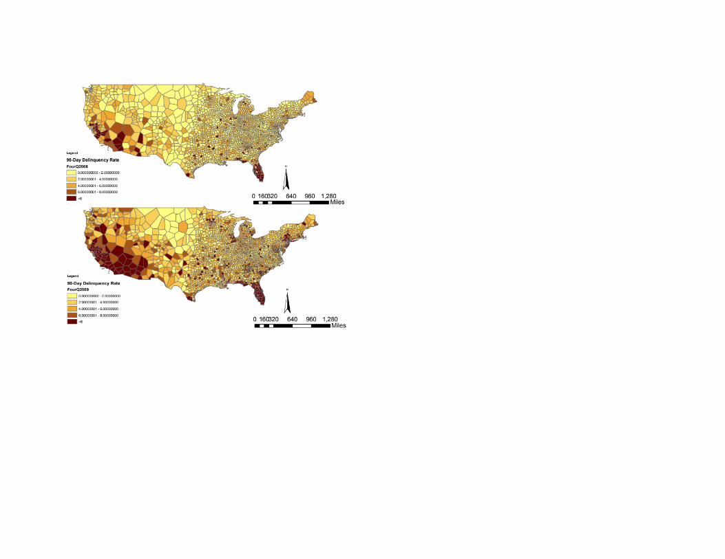
Local Indicators of Spatial Autocorrelation

Local Indicators of Spatial Autocorrelation (LISA) displaythe geographic areas in which the dependent variable showsstatistically significant autocorrelation. The LISA Maps(Figure 5) show that counties with high delinquency rateswere adjacent to other counties with high delinquency ratesin a relatively dispersed set of Thiessen polygons in theEastern half of the United States in 2006. However, over theperiod from 2007 to 2009, high-to-high spatialautocorrelation becomes concentrated in Florida and theSouthwest. Counties with low values were adjacent to othercounties with low values several of the Plains states, butconsistently so in Montana and North and South Dakota.

Figure 5.

Local Indicators of Spatial Autocorrelation

2006 2007

2008 2009

Hot Spot Analysis

Hot Spot Analysis was used to determine the areas in which spatialclustering was higher than would be expected in a random pattern(Figure 6). Spatial clustering differs from spatial autocorrelationin that statistically significant spatial clustering indicatessimilar values are concentrated in space due to some underlyingvariable, while spatial autocorrelation merely measures whetherthere is a correlation in the residuals. We see that hot spots wererelatively dispersed in 2006 and then become concentrated in Floridaand the Southwest over the period from 2007 to 2009.

Figure 6.

Local Getis-Ord Statistics

2006

2008

2007

2009

Spatial Regression Analysis

The spatial regression analysis began with estimating theHUD model against 90-day delinquency rates (Table 1). Thismodel included the unemployment rate, the percentage ofhigh-cost loans, and the OFHEO price change from peak.Several statistical problems were found with the HUD model.First, a Jarque-Bera test indicated the residuals were notnormally distributed, using a significance level of lessthan 0.001. The residuals also demonstratedheteroskedasticity in a White’s test, using a significancelevel of less than 0.001. Spatial statistical problems werealso present. Lagrange Multiplier tests indicated thatspatial lag and spatial error were present in the model,using a significance level of less than 0.001. These spatialproblems would lead one to inappropriately reject the nullhypothesis for one or more of the independent variables.Further, we see that even in the regular OLS model theunemployment rate was not a statistically significantpredictor of 90-day delinquency rates, once the percentageof high-cost loans and the OFHEO price change wereincorporated into the model.

Natural log transformations were used to eliminate theheteroskedasticity in the HUD model. For the OFHEO pricechange, a constant of 1 was added to the price change sothat negative values could be transformed into logs. Atfirst-order contiguity, this model did not demonstratespatial error. However, a Lagrange Multiplier test indicatedspatial lag was present, using a significance level of lessthan 0.001. The presence of spatial lag here indicates thatthe spatial autocorrelation in the residuals was due to anunderlying variable within the model. The most intuitiveexplanation is that the home price change was the source ofthe diffusion process.

The bottom portion of Table 1 displays the results forspatial lag models up to 13 orders of contiguity. Thecoefficient on LN (Price Change +1) was -3.009, and was

statistically significant at a significance level of lessthan 0.001. The coefficient on LN(High-Cost Loans) was0.616, and was statistically significant at a significancelevel of less than 0.001. The spatial lag (rho) coefficientwas 0.438. The unemployment rate was not significant.

The first-order spatial lag model results suggests we can becertain that there is a diffusion process operating forThiessen polygons that are directly adjacent to each other.This means the lag coefficient and corrected estimators forthe independent variables must be used in any model thatattempts to predict 90-day delinquency rates. The equationfor the model is as follows:

Ln(delinquency rate)i = -1.27 – 3.009*Ln(home price change+1)+0.616*Ln(high-cost loans) + 0.438(Wi,delinquency ratei ) + ε

Table 1. Regression Results

Theoretical Model

The null results for the unemployment variable suggests unemployment only affects county-level delinquency rates through its effect on the home price change. The home price change is also responsible for the diffusion process identified in the spatial regressions. Figure 7 presents a possible theoretical model for the process through which high delinquency rates spread from county to county. This draws upon and extends a theory suggested by Can (1998) on contagion effects in neighborhood foreclosures. First, unemployment and other unobserved economic variables affect home prices. Second, the home price change and the percentage of high-cost loans directly affect the delinquency rate. Third, some percentage of homes in delinquency move into foreclosure. Fourth, foreclosed homes are repriced at a discount. This repricing of foreclosed homes reduces home prices in adjacent counties. It is this repricing of the homes that is responsible for the diffusionof 90-day delinquencies.

Figure 7.Diffusion Process Theoretical Model

Statistical Conclusions We need to be cautious about interpreting the coefficientsdirectly. A Jarque-Bera test indicated that the residualswere not distributed normally in the HUD model or any of thealternative models. Further, the Lagrange Multiplier testresults in the models from 2 to 11 orders of contiguitysuggested spatial lag and spatial error may both be present.This may indicate that a SARMA model may be required infuture research to model the diffusion process at higherorders of contiguity. This does not seem to be a problem at12 orders of contiguity and above, as the spatialautocorrelation seems to be limited to regions.

The most assertive conclusion we can make at this point isthat the first-order spatial lag model produces betterestimators than the HUD model. We can also conclude that theunemployment rate provides no predictive power over andabove the home price change and the percentage of high costloans. This suggests NSP grantees would stop the diffusionprocess more efficiently if they targeted counties with the

steepest change in home prices and the largest percentage ofhigh-cost loans, regardless of the unemployment rate.

References

Anselin, Luc. (1998). “GIS Research Infrastructure for Spatial Analysis of Real Estate Markets.” Journal of Housing Research 9(1): 112-133.

Can, Ayse. (1998). “GIS and Spatial Analysis of Housing and Mortgage Markets.” Journal of Housing Research 9(1): 61-86.

Doms, Mark, Fred Furlong, and John Krainer. (2007). “Subprime Mortgage Delinquency Rates.” Working Paper 2007-33. Federal Reserve Bank of San Francisco. Retrieved from: http://www.frbsf.org/publications/economics/papers/2007/wp07-33bk.pdf

Hayre, Lakhbir (ed). (2001). Salomon Smith Barney Guide to Mortgage-backed and Asset-backed Securities. New York: John Wiley & Sons.

Schintler, Laurie, Emilia Istrate, Danilo Pelletiere, and Rajendra Kulkarni. (2010). "The Spatial Aspects of the Foreclosure Crisis: A look at the New England Region." Research Paper No. 2010-28. George Mason University School of Public Policy.

Taylor, John. (2007). “Housing and Monetary Policy.” SIEPR Discussion Paper No. 07-03. Stanford Institute for Economic Policy Research. Retrieved from: ftp://ftp.repec.org/opt/ReDIF/RePEc/sip/07-003.pdf

U.S. Department of Housing and Urban Development. Neighborhood Stabilization Program: Methodology and Data Dictionary for HUD-provided Data. October 20, 2008.

Retreived from: http://www.huduser.org/portal/datasets/nsp.html