Living Rev. Solar Phys., 7, (2010), 1 http://www.livingreviews.org/lrsp-2010-1 in solar physics LIVING REVIEWS The Solar Cycle David H. Hathaway Mail Code VP62, NASA Marshall Space Flight Center, Huntsville, AL 35812, U.S.A. email: [email protected] http://solarscience.msfc.nasa.gov/ Accepted on 21 February 2010 Published on 2 March 2010 Abstract The Solar Cycle is reviewed. The 11-year cycle of solar activity is characterized by the rise and fall in the numbers and surface area of sunspots. We examine a number of other solar activity indicators including the 10.7 cm radio flux, the total solar irradiance, the magnetic field, flares and coronal mass ejections, geomagnetic activity, galactic cosmic ray fluxes, and radioisotopes in tree rings and ice cores that vary in association with the sunspots. We examine the characteristics of individual solar cycles including their maxima and minima, cycle periods and amplitudes, cycle shape, and the nature of active latitudes, hemispheres, and longitudes. We examine long-term variability including the Maunder Minimum, the Gleissberg Cycle, and the Gnevyshev–Ohl Rule. Short-term variability includes the 154-day periodicity, quasi-biennial variations, and double peaked maxima. We conclude with an examination of prediction techniques for the solar cycle. This review is licensed under a Creative Commons Attribution-Non-Commercial-NoDerivs 3.0 Germany License. http://creativecommons.org/licenses/by-nc-nd/3.0/de/

Welcome message from author
This document is posted to help you gain knowledge. Please leave a comment to let me know what you think about it! Share it to your friends and learn new things together.
Transcript

Living Rev. Solar Phys., 7, (2010), 1http://www.livingreviews.org/lrsp-2010-1 in solar physics
L I V I N G REVIEWS
The Solar Cycle
David H. HathawayMail Code VP62,
NASA Marshall Space Flight Center,Huntsville, AL 35812, U.S.A.
email: [email protected]://solarscience.msfc.nasa.gov/
Accepted on 21 February 2010Published on 2 March 2010
Abstract
The Solar Cycle is reviewed. The 11-year cycle of solar activity is characterized by the riseand fall in the numbers and surface area of sunspots. We examine a number of other solaractivity indicators including the 10.7 cm radio flux, the total solar irradiance, the magneticfield, flares and coronal mass ejections, geomagnetic activity, galactic cosmic ray fluxes, andradioisotopes in tree rings and ice cores that vary in association with the sunspots. Weexamine the characteristics of individual solar cycles including their maxima and minima,cycle periods and amplitudes, cycle shape, and the nature of active latitudes, hemispheres, andlongitudes. We examine long-term variability including the Maunder Minimum, the GleissbergCycle, and the Gnevyshev–Ohl Rule. Short-term variability includes the 154-day periodicity,quasi-biennial variations, and double peaked maxima. We conclude with an examination ofprediction techniques for the solar cycle.
This review is licensed under a Creative CommonsAttribution-Non-Commercial-NoDerivs 3.0 Germany License.http://creativecommons.org/licenses/by-nc-nd/3.0/de/

Imprint / Terms of Use
Living Reviews in Solar Physics is a peer reviewed open access journal published by the Max PlanckInstitute for Solar System Research, Max-Planck-Str. 2, 37191 Katlenburg-Lindau, Germany. ISSN1614-4961.
This review is licensed under a Creative Commons Attribution-Non-Commercial-NoDerivs 3.0Germany License: http://creativecommons.org/licenses/by-nc-nd/3.0/de/
Because a Living Reviews article can evolve over time, we recommend to cite the article as follows:
David H. Hathaway,“The Solar Cycle”,
Living Rev. Solar Phys., 7, (2010), 1. [Online Article]: cited [<date>],http://www.livingreviews.org/lrsp-2010-1
The date given as <date> then uniquely identifies the version of the article you are referring to.
Article Revisions
Living Reviews supports two different ways to keep its articles up-to-date:
Fast-track revision A fast-track revision provides the author with the opportunity to add shortnotices of current research results, trends and developments, or important publications tothe article. A fast-track revision is refereed by the responsible subject editor. If an articlehas undergone a fast-track revision, a summary of changes will be listed here.
Major update A major update will include substantial changes and additions and is subject tofull external refereeing. It is published with a new publication number.
For detailed documentation of an article’s evolution, please refer always to the history documentof the article’s online version at http://www.livingreviews.org/lrsp-2010-1.

Contents
1 Introduction 5
2 The Solar Cycle Discovered 62.1 Schwabe’s discovery . . . . . . . . . . . . . . . . . . . . . . . . . . . . . . . . . . . 62.2 Wolf’s relative sunspot number . . . . . . . . . . . . . . . . . . . . . . . . . . . . . 72.3 Wolf’s reconstruction of earlier data . . . . . . . . . . . . . . . . . . . . . . . . . . 7
3 Solar Activity Data 93.1 Sunspot numbers . . . . . . . . . . . . . . . . . . . . . . . . . . . . . . . . . . . . . 93.2 Sunspot areas . . . . . . . . . . . . . . . . . . . . . . . . . . . . . . . . . . . . . . . 113.3 10.7 cm solar flux . . . . . . . . . . . . . . . . . . . . . . . . . . . . . . . . . . . . . 133.4 Total irradiance . . . . . . . . . . . . . . . . . . . . . . . . . . . . . . . . . . . . . . 143.5 Magnetic field . . . . . . . . . . . . . . . . . . . . . . . . . . . . . . . . . . . . . . . 173.6 Flares and Coronal Mass Ejections . . . . . . . . . . . . . . . . . . . . . . . . . . . 183.7 Geomagnetic activity . . . . . . . . . . . . . . . . . . . . . . . . . . . . . . . . . . . 193.8 Cosmic rays . . . . . . . . . . . . . . . . . . . . . . . . . . . . . . . . . . . . . . . . 213.9 Radioisotopes in tree rings and ice cores . . . . . . . . . . . . . . . . . . . . . . . . 24
4 Individual Cycle Characteristics 254.1 Minima and maxima . . . . . . . . . . . . . . . . . . . . . . . . . . . . . . . . . . . 254.2 Smoothing . . . . . . . . . . . . . . . . . . . . . . . . . . . . . . . . . . . . . . . . . 284.3 Cycle periods . . . . . . . . . . . . . . . . . . . . . . . . . . . . . . . . . . . . . . . 314.4 Cycle amplitudes . . . . . . . . . . . . . . . . . . . . . . . . . . . . . . . . . . . . . 324.5 Cycle shape . . . . . . . . . . . . . . . . . . . . . . . . . . . . . . . . . . . . . . . . 334.6 Rise time vs. amplitude (The Waldmeier Effect) . . . . . . . . . . . . . . . . . . . 344.7 Period vs. amplitude . . . . . . . . . . . . . . . . . . . . . . . . . . . . . . . . . . . 364.8 Active latitudes . . . . . . . . . . . . . . . . . . . . . . . . . . . . . . . . . . . . . . 364.9 Active hemispheres . . . . . . . . . . . . . . . . . . . . . . . . . . . . . . . . . . . . 374.10 Active longitudes . . . . . . . . . . . . . . . . . . . . . . . . . . . . . . . . . . . . . 40
5 Long-Term Variability 425.1 The Maunder Minimum . . . . . . . . . . . . . . . . . . . . . . . . . . . . . . . . . 425.2 The secular trend . . . . . . . . . . . . . . . . . . . . . . . . . . . . . . . . . . . . . 425.3 The Gleissberg Cycle . . . . . . . . . . . . . . . . . . . . . . . . . . . . . . . . . . . 435.4 Gnevyshev–Ohl Rule (Even–Odd Effect) . . . . . . . . . . . . . . . . . . . . . . . . 435.5 Long-term variations from radioisotope studies . . . . . . . . . . . . . . . . . . . . 445.6 The Suess cycle . . . . . . . . . . . . . . . . . . . . . . . . . . . . . . . . . . . . . . 44
6 Short-Term Variability 456.1 154-day periodicity . . . . . . . . . . . . . . . . . . . . . . . . . . . . . . . . . . . . 456.2 Quasi-biennial variations and double peaked maxima . . . . . . . . . . . . . . . . . 46
7 Solar Cycle Predictions 477.1 Predicting an ongoing cycle . . . . . . . . . . . . . . . . . . . . . . . . . . . . . . . 477.2 Predicting future cycle amplitudes based on cycle statistics . . . . . . . . . . . . . 477.3 Predicting future cycle amplitudes based on geomagnetic precursors . . . . . . . . 487.4 Predicting future cycle amplitudes based on dynamo theory . . . . . . . . . . . . . 53
8 Conclusions 56

References 57
List of Tables
1 Dates and values for sunspot cycle maxima. . . . . . . . . . . . . . . . . . . . . . . 262 Dates and values for sunspot cycle minima. The value is always the value of the
13-month mean of the International sunspot number. The dates differ according tothe indicator used. . . . . . . . . . . . . . . . . . . . . . . . . . . . . . . . . . . . . 27
3 Dates and values of maxima using the 13-month running mean with sunspot numberdata, sunspot area data, and 10.7 cm radio flux data. . . . . . . . . . . . . . . . . . 28
4 Dates and values of maxima using the 24-month FWHM Gaussian with sunspotnumber data, sunspot area data, and 10.7 cm radio flux data as in Table 3. . . . . 30
5 Cycle maxima determined by the 13-month mean with the International SunspotNumbers and the Group Sunspot Numbers. The Group values are systematicallylower than the International values prior to cycle 12. . . . . . . . . . . . . . . . . . 32
6 Prediction method errors for cycle 19 – 23. The three geomagnetic precursor methods(Ohl’s, Feynman’s, and Thompson’s) give the smallest errors. . . . . . . . . . . . . 52
The Solar Cycle 5
1 Introduction
Solar activity rises and falls with an 11-year cycle that affects us in many ways. Increased solaractivity includes increases in extreme ultraviolet and x-ray emissions from the Sun which producedramatic effects in the Earth’s upper atmosphere. The associated atmospheric heating increasesboth the temperature and density of the atmosphere at many spacecraft altitudes. The increasein atmospheric drag on satellites in low Earth orbit can dramatically shorten the lifetime of thesevaluable assets (cf. Pulkkinen, 2007).
Increases in the number of solar flares and coronal mass ejections (CMEs) raise the likelihoodthat sensitive instruments in space will be damaged by energetic particles accelerated in theseevents. These solar energetic particles (SEPs) can also threaten the health of both astronauts inspace and airline travelers in high altitude, polar routes.
Solar activity apparently affects terrestrial climate as well. Although the change in the totalsolar irradiance seems too small to produce significant climatic effects, there is good evidence that,to some extent, the Earth’s climate heats and cools as solar activity rises and falls (cf. Haigh,2007).
There is little doubt that the solar cycle is magnetic in nature and produced by dynamoprocesses within the Sun. Here we examine the nature of the solar cycle and the characteristicsthat must be explained by any viable dynamo model (cf. Charbonneau, 2005).
Living Reviews in Solar Physicshttp://www.livingreviews.org/lrsp-2010-1

6 David H. Hathaway
2 The Solar Cycle Discovered
Sunspots (dark patches on the Sun where intense magnetic fields loop up through the surface fromthe deep interior) were almost certainly seen by prehistoric humans viewing the Sun through hazyskies. The earliest actual recordings of sunspot observations were from China over 2000 years ago(Clark and Stephenson, 1978; Wittmann and Xu, 1987). Yet, the existence of spots on the Suncame as a surprise to westerners when telescopes were first used to observe the Sun in the early17th century. This is usually attributed to western philosophy in which the heavens and the Sunwere thought to be perfect and unblemished (cf. Bray and Loughhead, 1965; Noyes, 1982).
The first mention of possible periodic behavior in sunspots came from Christian Horrebow whowrote in his 1776 diary:
“Even though our observations conclude that changes of sunspots must be periodic, aprecise order of regulation and appearance cannot be found in the years in which itwas observed. That is because astronomers have not been making the effort to makeobservations of the subject of sunspots on a regular basis. Without a doubt, theybelieved that these observations were not of interest for either astronomy or physics.One can only hope that, with frequent observations of periodic motion of space objects,that time will show how to examine in which way astronomical bodies that are drivenand lit up by the Sun are influenced by sunspots.” (Wolf, 1877, translation by ElkeWillenberg)
2.1 Schwabe’s discovery
Although Christian Horrebow mentions this possible periodic variation in 1776 the solar (sunspot)cycle was not truly discovered until 1844. In that year Heinrich Schwabe reported in AstronomischeNachrichten (Schwabe, 1844) that his observations of the numbers of sunspot groups and spotlessdays over the previous 18-years indicated the presence of a cycle of activity with a period of about10 years. Figure 1 shows his data for the number of sunspot groups observed yearly from 1826 to1843.
1825 1830 1835 1840 1845Date
0
100
200
300
400
Su
ns
po
t G
rou
ps
Figure 1: Sunspot groups observed each year from 1826 to 1843 by Heinrich Schwabe (1844). These dataled Schwabe to his discovery of the sunspot cycle.
Living Reviews in Solar Physicshttp://www.livingreviews.org/lrsp-2010-1

The Solar Cycle 7
2.2 Wolf’s relative sunspot number
Schwabe’s discovery was probably instrumental in initiating the work of Rudolf Wolf (first atthe Bern Observatory and later at Zurich) toward acquiring daily observations of the Sun andextending the records to previous years (Wolf, 1861). Wolf recognized that it was far easier toidentify sunspot groups than to identify each individual sunspot. His “relative” sunspot number,𝑅, thus emphasized sunspot groups with
𝑅 = 𝑘 (10 𝑔 + 𝑛) (1)
where 𝑘 is a correction factor for the observer, 𝑔 is the number of identified sunspot groups, and 𝑛is the number of individual sunspots. These Wolf, Zurich, or International Sunspot Numbers havebeen obtained daily since 1849. Wolf himself was the primary observer from 1848 to 1893 and hada personal correction factor 𝑘 = 1.0. The primary observer has changed several times (Staudacherfrom 1749 to 1787, Flaugergues from 1788 to 1825, Schwabe from 1826 to 1847, Wolf from 1848 to1893, Wolfer from 1893 to 1928, Brunner from 1929 to 1944, and Waldmeier from 1945 to 1980).The Swiss Federal Observatory continued to provide sunspot numbers through 1980. Beginning in1981 and continuing through the present, the International Sunspot Number has been provided bythe Royal Observatory of Belgium with Koeckelenbergh as the primary observer (Solar InfluencesData Analysis Center - SIDC). Both Wolf and Wolfer observed the Sun in parallel over a 16-yearperiod. Wolf determined that the 𝑘-factor for Wolfer should be 𝑘 = 0.60 by comparing the sunspotnumbers calculated by Wolfer to those calculated by Wolf over the same days. In addition to theseprimary observers there were many secondary and tertiary observers whose observations were usedwhen those of the primary were unavailable. The process was changed from using the numbersfrom a single primary/secondary/tertiary observer to using a weighted average of many observerswhen the Royal Observatory of Belgium took over the process in 1981.
2.3 Wolf’s reconstruction of earlier data
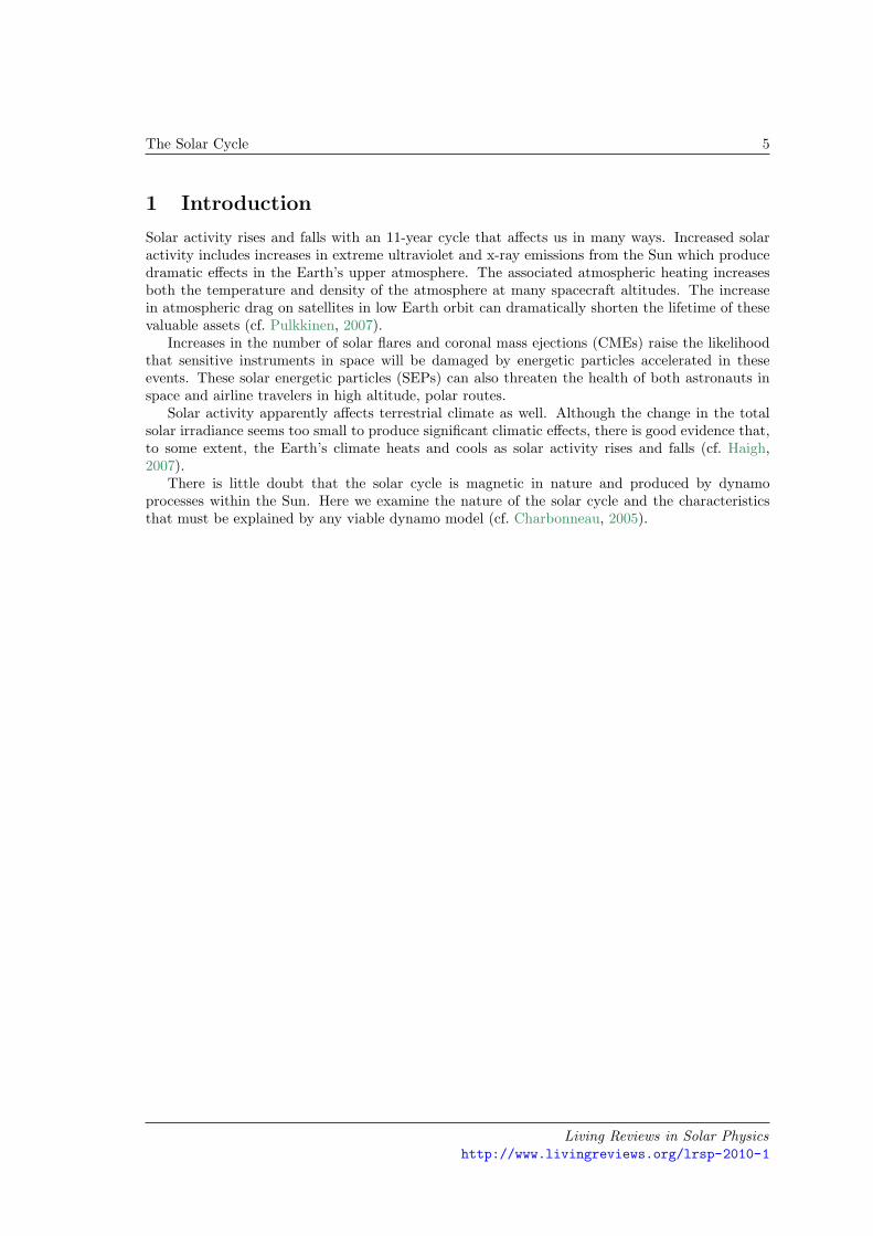
Wolf extended the data back to 1749 using the primary observers along with many secondaryobservers but much of that earlier data is incomplete. Wolf often filled in gaps in the sunspotobservations using geomagnetic activity measurements as proxies for the sunspot number. It iswell recognized that the sunspot numbers are quite reliable since Wolf’s time but that earliernumbers are far less reliable. The monthly averages of the daily numbers are shown in Figure 2.
Living Reviews in Solar Physicshttp://www.livingreviews.org/lrsp-2010-1
8 David H. Hathaway
Monthly Averaged Sunspot Numbers
1750 1760 1770 1780 1790 1800 1810 1820 1830 1840 1850 1860 1870 1880DATE
0
100
200
300
SU
NS
PO
T N
UM
BE
R
1 2 3 4 5 6 7 8 9 10 11
1880 1890 1900 1910 1920 1930 1940 1950 1960 1970 1980 1990 2000 2010DATE
0
100
200
300
SU
NS
PO
T N
UM
BE
R
12 13 14 15 16 17 18 19 20 21 22 23
Figure 2: Monthly averages of the daily International Sunspot Number. This illustrates the solar cycleand shows that it varies in amplitude, shape, and length. Months with observations from every day areshown in black. Months with 1 – 10 days of observation missing are shown in green. Months with 11 – 20days of observation missing are shown in yellow. Months with more than 20 days of observation missing areshown in red. [Missing days from 1818 to the present were obtained from the International daily sunspotnumbers. Missing days from 1750 to 1818 were obtained from the Group Sunspot Numbers and probablyrepresent an over estimate.]
Living Reviews in Solar Physicshttp://www.livingreviews.org/lrsp-2010-1

The Solar Cycle 9
3 Solar Activity Data
3.1 Sunspot numbers
The International Sunspot Number is the key indicator of solar activity. This is not becauseeveryone agrees that it is the best indicator but rather because of the length of the available record.Traditionally, sunspot numbers are given as daily numbers, monthly averages, yearly averages, andsmoothed numbers. The standard smoothing is a 13-month running mean centered on the monthin question and using half weights for the months at the start and end. Solar cycle maxima andminima are usually given in terms of these smoothed numbers.
Additional sunspot numbers do exist. The Boulder Sunspot Number is derived from the dailySolar Region Summary produced by the US Air Force and National Oceanic and AtmosphericAdministration (USAF/NOAA) from sunspot drawings obtained from the Solar Optical ObservingNetwork (SOON) sites since 1977. These summaries identify each sunspot group and list thenumber of spots in each group. The Boulder Sunspot Number is then obtained using Equation (1)with 𝑘 = 1.0. This Boulder Sunspot Number is typically about 55% larger than the InternationalSunspot Number (corresponding to a correction factor 𝑘 = 0.65) but is available promptly on adaily basis while the International Sunspot Number is posted monthly. The relationship betweenthe smoothed Boulder and International Sunspot Number is shown in Figure 3.
0 50 100 150 200
Smoothed International Number
0
50
100
150
200
250
Sm
oo
thed
Bo
uld
er N
um
ber
Figure 3: Boulder Sunspot Number vs. the International Sunspot Number at monthly intervals from1981 to 2007. The average ratio of the two is 1.55 and is represented by the solid line through the datapoints. The Boulder Sunspot Numbers can be brought into line with the International Sunspot Numbersby using a correction factor 𝑘 = 0.65 for Boulder.
A third sunspot number estimate is provided by the American Association of Variable Star Ob-servers (AAVSO) and is usually referred to as the American Sunspot Number. These numbers areavailable from 1944 to the present. While the American Number occasionally deviates systemati-cally from the International Number for years at a time it is usually kept closer to the InternationalNumber than the Boulder Number through its use of correction factors. (The American Number is
Living Reviews in Solar Physicshttp://www.livingreviews.org/lrsp-2010-1

10 David H. Hathaway
typically about 3% lower than the International Number.) The relationship between the Americanand International Sunspot number is shown in Figure 4.
0 50 100 150 200
Smoothed International Number
0
50
100
150
200
250
Sm
oo
thed
Am
eric
an
Nu
mb
er
Figure 4: American Sunspot Number vs. the International Sunspot Number at monthly intervals from1944 to 2006. The average ratio of the two is 0.97 and is represented by the solid line through the datapoints.
A fourth sunspot number is the Group Sunspot Number, 𝑅𝐺, devised by Hoyt and Schatten(1998). This index counts only the number of sunspot groups, averages together the observationsfrom multiple observers (rather than using the primary/secondary/tertiary observer system) andnormalizes the numbers to the International Sunspot Numbers using
𝑅𝐺 =12.08
𝑁
𝑁∑𝑖=1
𝑘𝑖𝐺𝑖 (2)
where 𝑁 is the number of observers, 𝑘𝑖 is the 𝑖-th observer’s correction factor, 𝐺𝑖 is the numberof sunspot groups observed by observer 𝑖, and 12.08 normalizes the number to the InternationalSunspot Number. Hathaway et al. (2002) found that the Group Sunspot Number follows theInternational Number fairly closely but not to the extent that it should supplant the InternationalNumber. In fact, the Group Sunspot Numbers are not readily available after 1995. The primaryutility of the Group Sunspot number is in extending the sunspot number observations back to theearliest telescopic observations in 1610. The relationship between the Group and InternationalSunspot number is shown in Figure 5 for the period 1874 to 1995. For this period the numbersagree quite well with the Group Number being about 1% higher than the International Number.For earlier dates the Group Number is a significant 24% lower than the International Number.
These sunspot numbers are available from NOAA. The International Number can be obtainedmonthly directly from SIDC.
Living Reviews in Solar Physicshttp://www.livingreviews.org/lrsp-2010-1

The Solar Cycle 11
0 50 100 150 200Smoothed International Number
0
50
100
150
200S
mo
oth
ed
Gro
up
Nu
mb
er
Figure 5: Group Sunspot Number vs. the International Sunspot Number at monthly intervals from 1874to 1995. The average ratio of the two is 1.01 and is represented by the solid line through the data points.
3.2 Sunspot areas
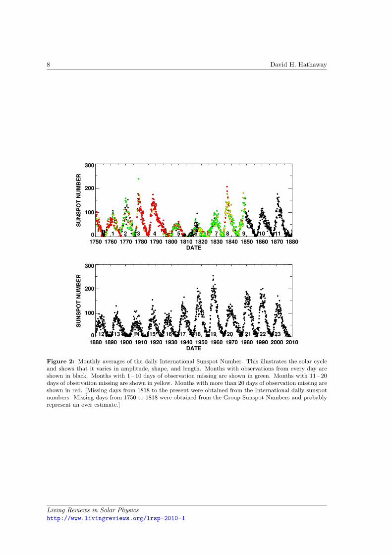
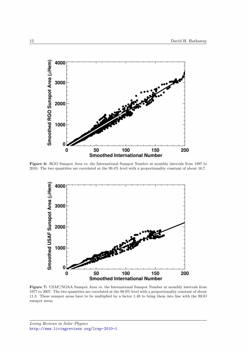
Sunspot areas are thought to be more physical measures of solar activity. Sunspot areas andpositions were diligently recorded by the Royal Observatory, Greenwich (RGO) from May of 1874to the end of 1976 using measurements off of photographic plates obtained from RGO itself and itssister observatories in Cape Town, South Africa, Kodaikanal, India, and Mauritius. Both umbralareas and whole spot areas were measured and corrected for foreshortening on the visible disc.Sunspot areas were given in units of millionths of a solar hemisphere (µHem). Comparing thecorrected whole spot areas to the International Sunspot Number (Figure 6) shows that the twoquantities are indeed highly correlated (𝑟 = 0.994, 𝑟2 = 0.988). Furthermore, there is no evidencefor any lead or lag between the two quantities over each solar cycle. Both measures could almostbe used interchangeably except for one aspect – the zero point. Since a single, solitary sunspotgives a sunspot number of 11 (6.6 for a correction factor 𝑘 = 0.6) the zero point for the sunspotnumber is shifted slightly from zero. The best fit to the data shown in Figure 6 gives an offset ofabout 4 and a slope of 16.7.
In 1977 NOAA began reporting much of the same sunspot area and position information in itsSolar Region Summary reports. These reports are derived from measurements taken from sunspotdrawings done at the USAF SOON sites. The sunspot areas were initially estimated by overlayinga grid and counting the number of cells that a sunspot covered. In late 1981 this procedure waschanged to employ an overlay with a number of circles and ellipses with different areas. Thesunspot areas reported by USAF/NOAA are significantly smaller than those from RGO (Fliggeand Solanki, 1997; Baranyi et al., 2001; Hathaway et al., 2002; Balmaceda et al., 2009). Figure 7shows the relationship between the USAF/NOAA sunspot areas and the International SunspotNumber. The slope in the straight line fit through the data is 11.32, significantly less than thatfound for the RGO sunspot areas. This indicates that these later sunspot area measurementsshould be multiplied by 1.48 to be consistent with the earlier RGO sunspot areas.
Living Reviews in Solar Physicshttp://www.livingreviews.org/lrsp-2010-1
12 David H. Hathaway
0 50 100 150 200Smoothed International Number
0
1000
2000
3000
4000
Sm
oo
the
d R
GO
Su
ns
po
t A
rea
(µ
He
m)
Figure 6: RGO Sunspot Area vs. the International Sunspot Number at monthly intervals from 1997 to2010. The two quantities are correlated at the 99.4% level with a proportionality constant of about 16.7.
0 50 100 150 200Smoothed International Number
0
1000
2000
3000
4000
Sm
oo
the
d U
SA
F S
un
sp
ot
Are
a (
µH
em
)
Figure 7: USAF/NOAA Sunspot Area vs. the International Sunspot Number at monthly intervals from1977 to 2007. The two quantities are correlated at the 98.9% level with a proportionality constant of about11.3. These sunspot areas have to be multiplied by a factor 1.48 to bring them into line with the RGOsunspot areas.
Living Reviews in Solar Physicshttp://www.livingreviews.org/lrsp-2010-1

The Solar Cycle 13
Sunspot areas are also available from a number of solar observatories including: Catania (1978 –1999), Debrecen (1986 – 1998), Kodaikanal (1906 – 1987), Mt. Wilson (1917 – 1985), Rome (1958 –2000), and Yunnan (1981 – 1992). While individual observatories have data gaps, their data arevery useful for helping to maintain consistency over the full interval from 1874 to the present.
The combined RGO USAF/NOAA datasets are available online (RGO).These datasets have additional information that is not reflected in sunspot numbers – positional
information – both latitude and longitude. The distribution of sunspot area with latitude (Figure 8)shows that sunspots appear in two bands on either side of the Sun’s equator. At the start of eachcycle spots appear at latitudes above about 20 – 25°. As the cycle progresses the range of latitudeswith sunspots broadens and the central latitude slowly drifts toward the equator, but with a zoneof avoidance near the equator. This behavior is referred to as “Sporer’s Law of Zones” by Maunder(1903) and was famously illustrated by his “Butterfly Diagram” (Maunder, 1904).
1870 1880 1890 1900 1910 1920 1930 1940 1950 1960 1970 1980 1990 2000 2010DATE
AVERAGE DAILY SUNSPOT AREA (% OF VISIBLE HEMISPHERE)
0.0
0.1
0.2
0.3
0.4
0.5
1870 1880 1890 1900 1910 1920 1930 1940 1950 1960 1970 1980 1990 2000 2010DATE
SUNSPOT AREA IN EQUAL AREA LATITUDE STRIPS (% OF STRIP AREA) > 0.0% > 0.1% > 1.0%
90S
30S
EQ
30N
90N
12 13 14 15 16 17 18 19 20 21 22 23
http://solarscience.msfc.nasa.gov/images/BFLY.pdf HATHAWAY/NASA/MSFC 2010/01
DAILY SUNSPOT AREA AVERAGED OVER INDIVIDUAL SOLAR ROTATIONS
Figure 8: Sunspot area as a function of latitude and time. The average daily sunspot area for each solarrotation since May 1874 is plotted as a function of time in the lower panel. The relative area in equalarea latitude strips is illustrated with a color code in the upper panel. Sunspots form in two bands, one ineach hemisphere, that start at about 25° from the equator at the start of a cycle and migrate toward theequator as the cycle progresses.
3.3 10.7 cm solar flux
The 10.7 cm Solar Flux is the disk integrated emission from the Sun at the radio wavelengthof 10.7 cm (2800 MHz) (cf. Tapping and Charrois, 1994). This measure of solar activity hasadvantages over sunspot numbers and areas in that it is completely objective and can be madeunder virtually all weather conditions. Measurements of this flux have been taken daily by theCanadian Solar Radio Monitoring Programme since 1946. Several measurements are taken eachday and care is taken to avoid reporting values influenced by flaring activity. Observations were
Living Reviews in Solar Physicshttp://www.livingreviews.org/lrsp-2010-1

14 David H. Hathaway
made in the Ottawa area from 1946 to 1990. In 1990 a new flux monitor was installed at Penticton,British Columbia and run in parallel with the Ottawa monitor for six months before moving theOttawa monitor itself to Penticton as a back-up. Measurements are provided daily (DRAO).
The relationship between the 10.7 cm radio flux and the International Sunspot Number issomewhat more complicated than that for sunspot area. First of all the 10.7 cm radio flux hasa base level of about 67 solar flux units. Secondly, the slope of the relationship changes as thesunspot number increases up to about 30. This is captured in a formula given by Holland andVaughn (1984) as:
𝐹10.7 = 67 + 0.97 𝑅𝐼 + 17.6(𝑒−0.035 𝑅𝐼 − 1
)(3)
In addition to this slightly nonlinear relationship there is evidence that the 10.7 cm radio flux lagsbehind the sunspot number by about 1-month (Bachmann and White, 1994).
0 50 100 150 200
Smoothed SSN
0
50
100
150
200
Sm
oo
thed
10.7
cm
Flu
x -
67.
Figure 9: 10.7cm Radio Flux vs. International Sunspot Number for the period of August 1947 to March2009. Data obtained prior to cycle 23 are shown with filled dots while data obtained during cycle 23 areshown with open circles. The Holland and Vaughn formula relating the radio flux to the sunspot numberis shown with the solid line. These two quantities are correlated at the 99.7% level.
Figure 9 shows the relationship between the 10.7 cm radio flux and the International SunspotNumber. The two measures are highly correlated (𝑟 = 0.995, 𝑟2 = 0.990). The Holland andVaughn formula fits the early data quite well. However, the data for cycle 23 after about 1998 liessystematically higher than the levels given by the Holland and Vaughn formula.
3.4 Total irradiance
The Total Solar Irradiance (TSI) is the radiant energy emitted by the Sun at all wavelengthscrossing a square meter each second outside the Earth’s atmosphere. Although ground-based mea-surements of this “solar constant” and its variability were made decades ago (Abbot et al., 1913),accurate measurements of the Sun’s total irradiance have only become available with access tospace. Several satellites have carried instruments designed to make these measurements: Nimbus-7 from November, 1978 to December, 1993; the Solar Maximum Mission (SMM) ACRIM-I from
Living Reviews in Solar Physicshttp://www.livingreviews.org/lrsp-2010-1

The Solar Cycle 15
February, 1980 to June, 1989; the Earth Radiation Budget Satellite (ERBS) from October, 1984 toDecember, 1995; NOAA-9 from January, 1985 to December, 1989; NOAA-10 from October, 1986to April, 1987; Upper Atmosphere Research Satellite (UARS) ACRIM-II from October, 1991 toNovember, 2001; ACRIMSAT ACRIM-III from December, 1999 to the present; SOHO/VIRGOfrom January, 1996 to the present; and SORCE/TIM from January, 2003 to the present.
While each of these instruments is extremely precise in its measurements, their absolute accura-cies vary in ways that make some important aspects of the TSI subjects of controversy. Figure 10shows daily measurements of TSI from some of these instruments. Each instrument measuresthe drops in TSI due to the formation and disk passages of large sunspot groups as well as thegeneral rise and fall of TSI with the sunspot cycle (Willson and Hudson, 1988). However, thereare significant offsets between the absolute measured values. Intercomparisons of the data havelead to different conclusions. Willson (1997) combined the SMM/ACRIM-I data with the laterUARS/ACRIM-II data by using intercomparisons with the Nimbus-7 and ERBS and concludedthat the Sun was brighter by about 0.04% during the cycle 22 minimum than is was during thecycle 21 minimum. Frohlich and Lean (1998) constructed a composite (the PMOD composite) thatincludes Nimbus-7, ERBS, SMM, UARS, and SOHO/VIRGO which does not show this increase.
1975 1980 1985 1990 1995 2000 2005 2010DATE
1360
1365
1370
1375
TS
I (W
m-2)
Nimbus 7
SMM/ACRIM
ERBS
SOHO/VIRGO
Figure 10: Daily measurements of the Total Solar Irradiance (TSI) from instruments on different satellites.The systematic offsets between measurements taken with different instruments complicate determinationsof the long-term behavior.
Comparing the PMOD composite to sunspot number (Figure 11) shows a strong correlationbetween the two quantities but with different behavior during cycle 23. At its peak, cycle 23 hadsunspot numbers about 20% smaller than cycle 21 or 22. However, the cycle 23 peak PMODcomposite TSI was similar to that of cycles 21 and 22. This behavior is similar to that seen in10.7 cm flux in Figure 9 but is complicated by the fact that the cycle 23 PMOD composite falls wellbelow that for cycle 21 and 22 during the decline of cycle 23 toward minimum while the 10.7 cmflux remained above the corresponding levels for cycles 21 and 22.
Living Reviews in Solar Physicshttp://www.livingreviews.org/lrsp-2010-1

16 David H. Hathaway
0 50 100 150 200
Smoothed International Number
0.0
0.5
1.0
1.5
2.0
Sm
oo
the
d T
SI-
13
65
.
Figure 11: The PMOD composite TSI vs. International Sunspot Number. The filled circles representsmoothed monthly averages for cycles 21 and 22. The open circles represent the data for cycle 23. Whilethe TSI at the minima preceding cycles 21 and 22 were similar in this composite, the TSI as cycle 23approaches minimum is significantly lower. The TSI at cycle 23 maximum was similar to that in cycles 21and 22 in spite of the fact that the sunspot number was significantly lower for cycle 23.
Living Reviews in Solar Physicshttp://www.livingreviews.org/lrsp-2010-1

The Solar Cycle 17
3.5 Magnetic field
Magnetic fields on the Sun were first measured in sunspots by Hale (1908). The magnetic natureof the solar cycle became apparent once these observations extended over more than a single cycle(Hale et al., 1919). Hale et al. (1919) provided the first description of “Hale’s Polarity Laws” forsunspots:
“. . . the preceding and following spots of binary groups, with few exceptions, are ofopposite polarity, and that the corresponding spots of such groups in the Northern andSouthern hemispheres are also of opposite sign. Furthermore, the spots of the presentcycle are opposite in polarity to those of the last cycle.”
Hale’s Polarity Laws are illustrated in Figure 12.
Figure 12: Hale’s Polarity Laws. A magnetogram from sunspot cycle 22 (1989 August 2) is shownon the left with yellow denoting positive polarity and blue denoting negative polarity. A correspondingmagnetogram from sunspot cycle 23 (2000 June 26) is shown on the right. Leading spots in one hemispherehave opposite magnetic polarity to those in the other hemisphere and the polarities flip from one cycle tothe next.
In addition to Hale’s Polarity Laws for sunspots, it was found that the Sun’s polar fields reverseas well. Babcock (1959) noted that the polar fields reversed at about the time of sunspot cyclemaximum. The Sun’s south polar field reversed in mid-1957 while its north polar field reversedin late-1958. The maximum for cycle 19 occurred in late-1957. The polar fields are thus out ofphase with the sunspot cycle – polar fields are at their peak near sunspot minimum. This is alsoindicated by the presence of polar faculae – small bright round patches seen in the polar regionsin white light observations of the Sun – whose number also peak at about the time of sunspotminimum (Sheeley Jr, 1991).
Systematic, daily observations of the Sun’s magnetic field over the visible solar disk were ini-tiated at the Kitt Peak National Observatory in the early 1970s. Synoptic maps from thesemeasurements are nearly continuous from early-1975 through mid-2003. Shortly thereafter simi-lar (and higher resolution) data became available from the National Solar Observatory’s SynopticOptical Long-term Investigations of the Sun (SOLIS) facility (Keller, 1998). Gaps between thesetwo datasets and within the SOLIS dataset can be filled with data from the Michelson Doppler
Living Reviews in Solar Physicshttp://www.livingreviews.org/lrsp-2010-1

18 David H. Hathaway
Imager (MDI) on the Solar and Heliospheric Observatory (SOHO) mission (Scherrer et al., 1995).These synoptic maps are presented in an animation here.
Figure 13: Still from a movie showing A full-disk magnetogram from NSO/KP used in constructingmagnetic synoptic maps over the last two sunspot cycles. Yellows represent magnetic field directed outward.Blues represent magnetic field directed inward. (To watch the movie, please go to the online version ofthis review article at http://www.livingreviews.org/lrsp-2010-1.)
The radial magnetic field averaged over longitude for each solar rotation is shown in Figure 14.This “Magnetic Butterfly Diagram” exhibits Hale’s Polarity Laws and the polar field reversals aswell as “Joy’s Law” (Hale et al., 1919):
“The following spot of the pair tends to appear farther from the equator than thepreceding spot, and the higher the latitude, the greater is the inclination of the axis tothe equator.”
Joy’s Law and Hale’s Polarity Laws are apparent in the “butterfly wings.” The equatorial sides ofthese wings are dominated by the lower latitude, preceding spot polarities while the poleward sidesare dominated by the higher latitude (due to Joy’s Law), following spot polarities. These polaritiesare opposite in opposite hemispheres and from one cycle to the next (Hale’s Law). This figure alsoshows that the higher latitude fields are transported toward the poles where they eventually reversethe polar field at about the time of sunspot cycle maximum.
3.6 Flares and Coronal Mass Ejections
Carrington (1859) and Hodgson (1859) reported the first observations of a solar flare from white-light observations on September 1, 1859. While observing the Sun projected onto viewing screenCarrington noticed a brightening that lasted for about 5 minutes. Hodgson also noted a nearlysimultaneous geomagnetic disturbance. Since that time flares have been observed in H-alpha frommany ground-based observatories and characterizations of flares from these observations have beenmade (cf. Benz, 2008).
X-rays from the Sun were measured by instruments on early rocket flights and their associationwith solar flares was recognized immediately. NOAA has flown solar x-ray monitors on its Geosta-tionary Operational Environmental Satellites (GOES) since 1975 as part of its Space Environment
Living Reviews in Solar Physicshttp://www.livingreviews.org/lrsp-2010-1

The Solar Cycle 19
90S
30S
EQ
30N
90N
La
titu
de
1975 1980 1985 1990 1995 2000 2005 2010
Date
-10G -5G 0G +5G+10G
Figure 14: A Magnetic Butterfly Diagram constructed from the longitudinally averaged radial magneticfield obtained from instruments on Kitt Peak and SOHO. This illustrates Hale’s Polarity Laws, Joy’s Law,polar field reversals, and the transport of higher latitude magnetic field elements toward the poles.
Monitor. The solar x-ray flux has been measured in two bandpasses by these instruments: 0.5to 4.0 A and 1.0 to 8.0 A. The x-ray flux is given on a logarithmic scale with A and B levels astypical background levels depending upon the phase of the cycle, and C, M, and X levels indicatingincreasing levels of flaring activity. The number of M-class and X-class flares seen in the 1.0 – 8.0 Aband tends to follow the sunspot number as shown in Figure 15. The two measures are well cor-related (𝑟 = 0.948, 𝑟2 = 0.900) but there is a tendency to have more flares on the declining phaseof a sunspot cycle (the correlation is maximized for a 2-month lag). In spite of this correlation,significant flares can, and have, occurred at all phases of the sunspot cycle. X-class flares haveoccurred during the few months surrounding sunspot cycle minimum for all of the cycles observedthus far (Figure 15).
Coronal mass ejections (CMEs) are often associated with flares but can also occur in theabsence of a flare. CMEs were discovered in the early 1970s from spacecraft observations fromOSO 7 (Tousey, 1973) and from Skylab (MacQueen et al., 1974). Routine CME observationsbegan with the Solar Maximum Mission and continue with SOHO. The frequency of occurrenceof CME’s is also correlated with sunspot number (Webb and Howard, 1994).
3.7 Geomagnetic activity
Geomagnetic activity also shows a solar cycle dependence but one that is more complex than seenin sunspot area, radio flux, or flares and CMEs. There are a number of indices of geomagneticactivity, most measure rapid (hour-to-hour) changes in the strength and/or direction of the Earth’smagnetic field from small networks of ground-based observatories. The ap index is a measure ofthe range of variability in the geomagnetic field (in 2 nT units) measured in three-hour intervalsfrom a network of about 13 high latitude stations. The average of the eight daily ap values isgiven as the equivalent daily amplitude Ap. These indices extend from 1932 to the present. Theaa index extends back further (to 1868 cf. Mayaud, 1972). It is similarly derived from three-hourintervals but from two antipodal stations located at latitudes of about 50°. The locations of thesetwo stations have changed from time to time and there is evidence (Svalgaard et al., 2004) thatthese changes are reflected in the data itself. Another frequently used index is Dst, disturbance
Living Reviews in Solar Physicshttp://www.livingreviews.org/lrsp-2010-1

20 David H. Hathaway
0 50 100 150 200Smoothed Sunspot Number
0
10
20
30
40
50
60
Sm
oo
thed
Mo
nth
ly F
lare
s (
M +
X)
Figure 15: Monthly M- and X-class flares vs. International Sunspot Number for the period of March1976 to January 2010. These two quantities are correlated at the 94.8% level but show significant scatterwhen the sunspot number is high (greater than ∼ 100).
1975 1980 1985 1990 1995 2000 2005 2010
Date
0
50
100
150
200
Sm
oo
the
d I
nte
rn
ati
on
al
Nu
mb
er
1-2 X Flares 3-9 X Flares 10+ X Flares
Figure 16: Monthly X-class flares and International Sunspot Number. X-class flares can occur at anyphase of the sunspot cycle – including cycle minimum.
Living Reviews in Solar Physicshttp://www.livingreviews.org/lrsp-2010-1

The Solar Cycle 21
storm time, derived from measurements obtained at four equatorial stations since 1957.Figure 17 shows the smoothed monthly geomagnetic index aa as a function of time along
with the sunspot number for comparison. The minima in geomagnetic activity tend to occur justafter those for the sunspot number and the geomagnetic activity tends to remain high during thedeclining phase of each cycle. This late cycle geomagnetic activity is attributed to the effectsof high-speed solar wind streams from low-latitude coronal holes (cf. Legrand and Simon, 1985).Figure 17 also shows the presence of multi-cycle trends in geomagnetic activity that may be relatedto changes in the Sun’s magnetic field (Lockwood et al., 1999).
Feynman (1982) decomposed geomagnetic variability into two components – one proportionalto and in phase with the sunspot cycle (the R, or Relative sunspot number component) andanother out of phase with the sunspot cycle (the I, or Interplanetary component). Figure 18shows the relationship between geomagnetic activity and sunspot number. As the sunspot numberincreases there is an increasing baseline level of geomagnetic activity. Feynman’s R componentis determined by finding this baseline level of geomagnetic activity by fitting a line proportionalto Sunspot Number. The I component is then the remaining geomagnetic activity. These twocomponents are plotted separately in Figure 19.
1880 1900 1920 1940 1960 1980 2000Date
0
10
20
30
40
Ge
om
ag
ne
tic
aa
In
de
x (
SS
N/5
)
Figure 17: Geomagnetic activity and the sunspot cycle. The geomagnetic activity index aa is plotted inred. The sunspot number (divided by five) is plotted in black.
3.8 Cosmic rays
The flux of galactic cosmic rays at 1 AU is modulated by the solar cycle. Galactic cosmic raysconsist of electrons and bare nuclei accelerated to GeV energies and higher at shocks produced bysupernovae. The positively charged nuclei produce cascading showers of particles in the Earth’supper atmosphere that can be measured by neutron monitors at high altitude observing sites.The oldest continuously operating neutron monitor is located at Climax, Colorado, USA. Dailyobservations extend from 1951 to 2006. Monthly averages of the neutron counts are shown as a
Living Reviews in Solar Physicshttp://www.livingreviews.org/lrsp-2010-1

22 David H. Hathaway
0 50 100 150 200Smoothed International Number
0
10
20
30
40
Sm
oo
thed
Geo
mag
neti
c In
dex a
a (
nT
)
Figure 18: Geomagnetic activity index aa vs. Sunspot Number. As Sunspot Number increases thebaseline level of geomagnetic activity increases as well.
1860 1880 1900 1920 1940 1960 1980 2000Date
0
5
10
15
20
25
30
35
Ge
om
ag
ne
tic
aa
In
de
x (
nT
)
aaR = 10.9 + 0.097 RaaI = aa - aaR
11
1213
14
1516
17
18
19
20
21 22
23
Figure 19: The smoothed R- and I-components of the geomagnetic index aa.
Living Reviews in Solar Physicshttp://www.livingreviews.org/lrsp-2010-1

The Solar Cycle 23
function of time in Figure 20 along with the sunspot number. As the sunspot numbers rise theneutron counts fall. This anti-correlation is attributed to scattering of the cosmic rays by tangledmagnetic field within the heliosphere (Parker, 1965). At times of high solar activity magneticstructures are carried outward on the solar wind. These structures scatter cosmic rays and reducetheir flux in the inner solar system.
The reduction in cosmic ray flux tends to lag behind solar activity by 6- to 12-months (Forbush,1954) but with significant differences between the even numbered and odd numbered cycles. Inthe even numbered cycles (cycles 20 and 22) the cosmic ray variations seen by neutron monitorslag sunspot number variations by only about 2-months. In the odd numbered cycles (cycles 19,21, and 23) the lag is from 10 to 14 months. Figure 20 also shows that the shapes of the cosmicray maxima at sunspot cycle minima are different for the even and odd numbered cycles. Thecosmic ray maxima (as measured by the neutron monitors) are sharply peaked at the sunspotcycle minima leading up to even numbered cycles and broadly peaked prior to odd numberedsunspot cycles. This behavior is accounted for in the transport models for galactic cosmic raysin the heliosphere (cf. Ferreira and Potgieter, 2004). The positively charged cosmic rays drift infrom the heliospheric polar regions when the Sun’s north polar field is directed outward (positive).When the Sun’s north polar field is directed inward (negative) the positively charged cosmic raysdrift inward along the heliospheric current sheet where they are scattered by corrugations in thecurrent sheet and by magnetic clouds from CME’s. The negatively charged cosmic rays (electrons)drift inward from directions (polar or equatorial) opposite to the positively charged cosmic raysthat are detected by neutron monitors.
1950 1960 1970 1980 1990 2000 2010Date
3000
3500
4000
4500
5000
5500
6000
Clim
ax C
osm
ic R
ay F
lux
A+ A- A+ A- A+ A-
Figure 20: Cosmic Ray flux from the Climax Neutron Monitor and rescaled Sunspot Number. Themonthly averaged neutron counts from the Climax Neutron Monitor are shown by the solid line. Themonthly averaged sunspot numbers (multiplied by five and offset by 4500) are shown by the dotted line.Cosmic ray variations are anti-correlated with solar activity but with differences depending upon the Sun’sglobal magnetic field polarity (A+ indicates periods with positive polarity north pole while A– indicatesperiods with negative polarity).
Living Reviews in Solar Physicshttp://www.livingreviews.org/lrsp-2010-1

24 David H. Hathaway
3.9 Radioisotopes in tree rings and ice cores
The radioisotopes 14C and 10Be are produced in the Earth’s stratosphere by the impact of galacticcosmic rays on 14N and 16O. The 14C gets oxidized to form CO2 which is taken up by plantsin general and trees in particular where it becomes fixed in annual growth rings. The 10Be getsoxidized and becomes attached to aerosols that can precipitate in snow where it then becomesfixed in annual layers of ice. The solar cycle modulation of the cosmic ray flux can then lead tosolar cycle related variations in the atmospheric abundances of 14C (Stuiver and Quay, 1980) and10Be (Beer et al., 1990). While the production rates of these two radioisotopes in the stratosphereshould be anti-correlated with the sunspot cycle, the time scales involved in the transport andultimate deposition in tree rings and ice tends to reduce and delay the solar cycle variations (cf.Masarik and Beer, 1999). Furthermore, the production rates in the stratospheric are functionsof latitude and changes to the Earth’s magnetic dipole moment and the latency in the strato-sphere/troposphere is a function of the changing reservoirs for these chemical species. This rathercomplicated production/transport/storage/deposition process makes direct comparisons betweenΔ14C (basically the difference between measured 14C abundance and that expected from its 5730year half-life) and sunspot number difficult.
Living Reviews in Solar Physicshttp://www.livingreviews.org/lrsp-2010-1

The Solar Cycle 25
4 Individual Cycle Characteristics
Each sunspot cycle has its own characteristics. Many of these characteristics are shared by othercycles and these shared characteristics provide important information for models of the solar activ-ity cycle. A paradigm shift in sunspot cycle studies came about when Waldmeier (1935) suggestedthat each cycle should be treated as an individual outburst with its own characteristics. Priorto that time, the fashion was to consider solar activity as a superposition of Fourier components.This superposition idea probably had its roots in the work of Wolf (1859) who suggested a formulabased on the orbits of Venus, Earth, Jupiter, and Saturn to fit Schwabe’s data for the years 1826to 1848.
Determining characteristics such as period and amplitude would seem simple and straight for-ward but the published studies show that this is not true. A prime example concerns determinationsof the dates (year and month) of cycle minima. A frequently used method is to take monthly av-erages of the daily International Sunspot Number and to smooth these with the 13-month runningmean. Unfortunately, this leaves several uncertain dates. With this method, the minimum thatoccurred in 1810 prior to cycle 6 could be taken as any month from April to December – all ninemonths had smoothed sunspot numbers of 0.0!
4.1 Minima and maxima
The dates and values for the cycle minima and maxima are the primary data for many studies ofthe solar cycle. These data are sensitive to the methods and input data used to find them. Solaractivity is inherently noisy and it is evident that there are significant variations in solar activityon time scales shorter than 11 years (see Section 7). Waldmeier (1961) published tables of sunspotnumbers along with dates and values of minima and maxima for cycles 1 to 19. McKinnon (1987)extended the data to include cycles 20 and 21. The values they give for sunspot number maximaand minima are those found using the 13-month running mean. However, the dates given formaxima and minima may vary after considering additional indicators. According to McKinnon:
“. . . maximum is based in part on an average of the times extremes are reached in themonthly mean sunspot number, the smoothed monthly mean sunspot number, and inthe monthly mean number of spot groups alone.”
These dates and the values for sunspot cycle maxima are given in Table 1 (the number of groups ismultiplied by 12.08 to produce group sunspot numbers that are comparable to the relative sunspotnumbers). It is clear from this table that considerably more weight is given to the date providedby the 13-month running mean. The dates provided by Waldmeier and McKinnon are far closerto those given by the 13-month running mean than they are to the average date of the threeindicators. (One exception is the date they give for the maximum of cycle 14 which should be halfa year earlier by almost any averaging scheme.) The monthly numbers of sunspots and spot groupsvary widely and, in fact, should be less reliable indicators and given lesser weight in determiningmaximum.
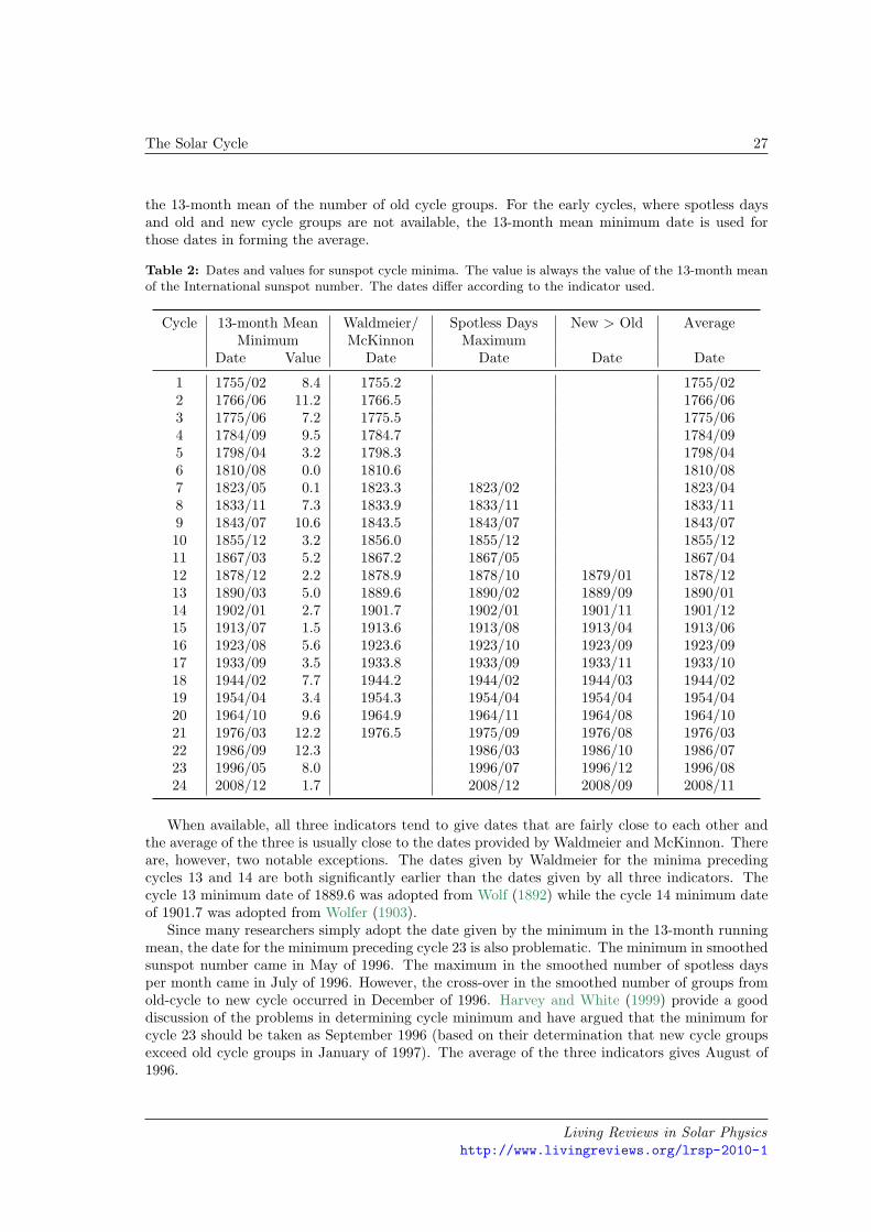
The minima in these three indicators have been used along with additional sunspot indicatorsto determine the dates of minima. The number of spotless days in a month tends to maximize atthe time of minimum and the number of new cycle sunspot groups begins to exceed the number ofold cycle sunspot groups at the time of minimum. Both Waldmeier and McKinnon suggest usingthese indicators as well when setting the dates for minima. These dates are given in Table 2 whereboth the spotless days per month and the number of old cycle and new cycle groups per monthare smoothed with the same 13-month mean filter. The average date given in the last column isthe average of the 13-month mean minimum date, the 13-month mean spotless days per monthmaximum date, and the date when the 13-month mean of the number of new cycle groups exceeds
Living Reviews in Solar Physicshttp://www.livingreviews.org/lrsp-2010-1

26 David H. Hathaway
Table 1: Dates and values for sunspot cycle maxima.
Cycle Waldmeier/McKinnon
13-month MeanMaximum
Monthly MeanMaximum
Monthly GroupMaximum
Date Value Date Value Date Value Date Value
1 1761.5 86.5 1761/06 86.5 1761/05 107.2 1761/05 109.42 1769.7 115.8 1769/09 115.8 1769/10 158.2 1771/05 162.53 1778.4 158.5 1778/05 158.5 1778/05 238.9 1778/01 144.04 1788.1 141.2 1788/02 141.2 1787/12 174.0 1787/12 169.05 1805.2 49.2 1805/02 49.2 1804/10 62.3 1805/11 67.06 1816.4 48.7 1816/05 48.7 1817/03 96.2 1817/03 57.07 1829.9 71.7 1829/11 71.5 1830/04 106.3 1830/04 101.58 1837.2 146.9 1837/03 146.9 1836/12 206.2 1837/01 160.79 1848.1 131.6 1848/02 131.9 1847/10 180.4 1849/01 130.910 1860.1 97.9 1860/02 98.0 1860/07 116.7 1860/07 103.411 1870.6 140.5 1870/08 140.3 1870/05 176.0 1870/05 122.312 1883.9 74.6 1883/12 74.6 1882/04 95.8 1884/01 86.013 1894.1 87.9 1894/01 87.9 1893/08 129.2 1893/08 126.714 1907.0? 64.2 1906/02 64.2 1907/02 108.2 1906/07 111.615 1917.6 105.4 1917/08 105.4 1917/08 154.5 1917/08 157.016 1928.4 78.1 1928/04 78.1 1929/12 108.0 1929/12 121.817 1937.4 119.2 1937/04 119.2 1938/07 165.3 1937/02 154.518 1947.5 151.8 1947/05 151.8 1947/05 201.3 1947/07 149.319 1957.9 201.3 1958/03 201.3 1957/10 253.8 1957/10 222.220 1968.9 110.6 1968/11 110.6 1969/03 135.8 1968/05 132.321 1979.9 164.5 1979/12 164.5 1979/09 188.4 1979/01 179.422 1989/07 158.5 1990/08 200.3 1990/08 195.923 2000/04 120.7 2000/07 169.1 2000/07 153.9
Living Reviews in Solar Physicshttp://www.livingreviews.org/lrsp-2010-1
The Solar Cycle 27
the 13-month mean of the number of old cycle groups. For the early cycles, where spotless daysand old and new cycle groups are not available, the 13-month mean minimum date is used forthose dates in forming the average.
Table 2: Dates and values for sunspot cycle minima. The value is always the value of the 13-month meanof the International sunspot number. The dates differ according to the indicator used.
Cycle 13-month MeanMinimum
Waldmeier/McKinnon
Spotless DaysMaximum
New > Old Average
Date Value Date Date Date Date
1 1755/02 8.4 1755.2 1755/022 1766/06 11.2 1766.5 1766/063 1775/06 7.2 1775.5 1775/064 1784/09 9.5 1784.7 1784/095 1798/04 3.2 1798.3 1798/046 1810/08 0.0 1810.6 1810/087 1823/05 0.1 1823.3 1823/02 1823/048 1833/11 7.3 1833.9 1833/11 1833/119 1843/07 10.6 1843.5 1843/07 1843/0710 1855/12 3.2 1856.0 1855/12 1855/1211 1867/03 5.2 1867.2 1867/05 1867/0412 1878/12 2.2 1878.9 1878/10 1879/01 1878/1213 1890/03 5.0 1889.6 1890/02 1889/09 1890/0114 1902/01 2.7 1901.7 1902/01 1901/11 1901/1215 1913/07 1.5 1913.6 1913/08 1913/04 1913/0616 1923/08 5.6 1923.6 1923/10 1923/09 1923/0917 1933/09 3.5 1933.8 1933/09 1933/11 1933/1018 1944/02 7.7 1944.2 1944/02 1944/03 1944/0219 1954/04 3.4 1954.3 1954/04 1954/04 1954/0420 1964/10 9.6 1964.9 1964/11 1964/08 1964/1021 1976/03 12.2 1976.5 1975/09 1976/08 1976/0322 1986/09 12.3 1986/03 1986/10 1986/0723 1996/05 8.0 1996/07 1996/12 1996/0824 2008/12 1.7 2008/12 2008/09 2008/11
When available, all three indicators tend to give dates that are fairly close to each other andthe average of the three is usually close to the dates provided by Waldmeier and McKinnon. Thereare, however, two notable exceptions. The dates given by Waldmeier for the minima precedingcycles 13 and 14 are both significantly earlier than the dates given by all three indicators. Thecycle 13 minimum date of 1889.6 was adopted from Wolf (1892) while the cycle 14 minimum dateof 1901.7 was adopted from Wolfer (1903).
Since many researchers simply adopt the date given by the minimum in the 13-month runningmean, the date for the minimum preceding cycle 23 is also problematic. The minimum in smoothedsunspot number came in May of 1996. The maximum in the smoothed number of spotless daysper month came in July of 1996. However, the cross-over in the smoothed number of groups fromold-cycle to new cycle occurred in December of 1996. Harvey and White (1999) provide a gooddiscussion of the problems in determining cycle minimum and have argued that the minimum forcycle 23 should be taken as September 1996 (based on their determination that new cycle groupsexceed old cycle groups in January of 1997). The average of the three indicators gives August of1996.
Living Reviews in Solar Physicshttp://www.livingreviews.org/lrsp-2010-1

28 David H. Hathaway
Additional problems in assigning dates and values to maxima and minima can be seen whenusing data other than sunspot numbers. Table 3 lists the dates and values for cycle maxima usingthe 13-month running mean on sunspot numbers, sunspot areas, and 10.7 cm radio flux. Thesunspot areas have been converted to sunspot number equivalents using the relationship shownin Figure 6 and the 10.7 cm radio flux has been converted into sunspot number equivalents usingEquation (3). Very significant differences can be seen in the dates. Over the last five cycles theranges in dates given by the different indices have been: 4, 27, 25, 1, and 22 months.
Table 3: Dates and values of maxima using the 13-month running mean with sunspot number data,sunspot area data, and 10.7 cm radio flux data.
Cycle 13-month MeanMaximum
13-month MeanSunspot Area
13-month Mean10.7 cm Flux
Date Value Date R-Value Date R-Value
1 1761/06 86.52 1769/09 115.83 1778/05 158.54 1788/02 141.25 1805/02 49.26 1816/05 48.77 1829/11 71.58 1837/03 146.99 1848/02 131.910 1860/02 98.011 1870/08 140.312 1883/12 74.6 1883/11 88.313 1894/01 87.9 1894/01 100.414 1906/02 64.2 1905/06 75.415 1917/08 105.4 1917/08 93.016 1928/04 78.1 1926/04 92.317 1937/04 119.2 1937/05 133.318 1947/05 151.8 1947/05 166.519 1958/03 201.3 1957/11 216.5 1958/03 201.220 1968/11 110.6 1968/04 100.9 1970/07 109.621 1979/12 164.5 1982/01 156.0 1981/05 159.422 1989/07 158.5 1989/06 158.5 1989/06 168.023 2000/04 120.7 2002/02 126.7 2002/02 152.3
These tables illustrate the problems in determining dates and values for cycle minima andmaxima. The crux of the problem is in the short-term variability of solar activity. One solution isto use different smoothing.
4.2 Smoothing
The monthly averages of the daily International Sunspot Number are noisy and must be smoothedin some manner in order to determine appropriate values for parameters such as minima, maxima,and their dates of occurrence. The daily values themselves are relatively uncertain. They dependupon the number and the quality of observations as well as the time of day when they are taken(the sunspot number changes over the course of the day as spots form and fade away). The monthlyaverages of these daily values are also problematic. The Sun rotates once in about 27-days but the
Living Reviews in Solar Physicshttp://www.livingreviews.org/lrsp-2010-1

The Solar Cycle 29
months vary in length from 28 to 31 days. If the Sun is particularly active at one set of longitudesthen some monthly averages will include one appearance of these active longitudes while othermonths will include two. This aspect is particularly important for investigations of short-term(months) variability (see Section 7). For long-term (years) variability this can be treated as noiseand filtered out.
The traditional 13-month running mean (centered on a given month with equal weights formonths –5 to +5 and half weight for months –6 and +6) is both simple and widely used butdoes a poor job of filtering out high frequency variations (although it is better than the simple12-month average). Gaussian shaped filters are preferable because they have Gaussian shapes inthe frequency domain and effectively remove high frequency variations (Hathaway et al., 1999). Atapered (to make the filter weights and their first derivatives vanish at the end points) Gaussianfilter is given by
𝑊 (𝑡) = 𝑒−𝑡2/2𝑎2− 𝑒−2
(3− 𝑡2/2𝑎2
)(4)
with
− 2𝑎 + 1 ≤ 𝑡 ≤ +2𝑎− 1 (5)
where 𝑡 is the time in months and 2𝑎 is the FWHM of the filter (note that this formula is slightlydifferent than that given in Hathaway et al. (1999). There are significant variations in solar activityon time scales of one to three years (see Section 7). These variations can produce double peakedmaxima which are filtered out by a 24-month Gaussian filter. The frequency responses of thesefilters are shown in Figure 21.
0 1 2 3 4 5 6Frequency (cycles/year)
0.001
0.010
0.100
1.000
Sig
na
l T
ran
sm
iss
ion
13-Month Running Mean12-Month Average24-Month FWHM Gaussian
Figure 21: Signal transmission for filters used to smooth monthly sunspot numbers. The 13-month run-ning mean and the 12-month average pass significant fractions (as much as 20%) of signals with frequencieshigher than 1/year. The 24-month FWHM Gaussian passes less than 0.3% of those frequencies and passesless than about 1% of the signal with frequencies of 1/2-years or higher.
Using the 24-month FWHM Gaussian filter on the data used to create Table 3 gives far moreconsistent results for both maxima and minima. The results for maxima are shown in Table 4.The ranges of dates for the last five maxima become: 1, 10, 13, 4, and 11 months – roughly halfthe ranges found using the 13-month running mean.
Living Reviews in Solar Physicshttp://www.livingreviews.org/lrsp-2010-1

30 David H. Hathaway
Table 4: Dates and values of maxima using the 24-month FWHM Gaussian with sunspot number data,sunspot area data, and 10.7 cm radio flux data as in Table 3.
Cycle 24-monthGaussianMaximum
24-MonthGaussian
Sunspot Area
24-MonthGaussian
10.7 cm FluxDate Value Date R-Value Date R-Value
1 1761/05 72.92 1770/01 100.53 1778/09 137.44 1788/03 130.65 1804/06 45.76 1816/08 43.87 1829/10 67.18 1837/04 146.99 1848/06 115.710 1860/03 92.111 1870/11 138.512 1883/11 64.7 1883/10 70.813 1893/09 81.4 1893/09 84.714 1906/05 59.6 1906/04 62.415 1917/12 88.6 1918/01 79.616 1927/12 71.6 1926/12 75.917 1937/11 108.2 1938/02 118.118 1948/03 141.7 1947/09 140.019 1958/02 188.0 1958/03 192.0 1958/03 188.120 1969/03 106.6 1968/09 95.5 1969/07 104.621 1980/05 151.8 1981/06 140.2 1980/11 153.122 1990/02 149.2 1990/06 141.7 1990/06 156.123 2000/12 112.7 2001/11 106.2 2001/06 136.4
Living Reviews in Solar Physicshttp://www.livingreviews.org/lrsp-2010-1
The Solar Cycle 31
4.3 Cycle periods
The period of a sunspot cycle is defined as the elapsed time from the minimum preceding itsmaximum to the minimum following its maximum. This does not, of course, account for thefact that each cycle actually starts well before its preceding minimum and continues long after itsfollowing minimum. By this definition, a cycle’s period is dependent upon the behavior of both thepreceding and following cycles. The measured period of a cycle is also subject to the uncertaintiesin determining the dates of minimum as indicated in the previous subsections. Nonetheless, thelength of a sunspot cycle is a key characteristic and variations in cycle periods have been wellstudied. The average cycle period can be fairly accurately determined by simply subtracting thedate for the minimum preceding cycle 1 from the date for the minimum preceding cycle 23 anddividing by the 22 cycles those dates encompass. This gives an average period for cycles 1 to 22of 131.7 months – almost exactly 11 years.
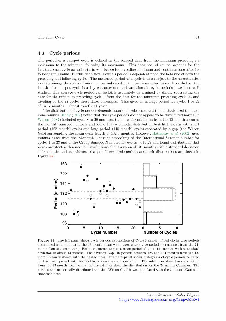
The distribution of cycle periods depends upon the cycles used and the methods used to deter-mine minima. Eddy (1977) noted that the cycle periods did not appear to be distributed normally.Wilson (1987) included cycle 8 to 20 and used the dates for minimum from the 13-month mean ofthe monthly sunspot numbers and found that a bimodal distribution best fit the data with shortperiod (122 month) cycles and long period (140 month) cycles separated by a gap (the WilsonGap) surrounding the mean cycle length of 132.8 months. However, Hathaway et al. (2002) usedminima dates from the 24-month Gaussian smoothing of the International Sunspot number forcycles 1 to 23 and of the Group Sunspot Numbers for cycles –4 to 23 and found distributions thatwere consistent with a normal distributions about a mean of 131 months with a standard deviationof 14 months and no evidence of a gap. These cycle periods and their distributions are shown inFigure 22.
0 5 10 15 20 0 5 10 Cycle Number Number of Cycles
96
108
120
132
144
156
168
Pe
rio
d (
mo
nth
s)
Figure 22: The left panel shows cycle periods as functions of Cycle Number. Filled circles give periodsdetermined from minima in the 13-month mean while open circles give periods determined from the 24-month Gaussian smoothing. Both measurements give a mean period of about 131 months with a standarddeviation of about 14 months. The “Wilson Gap” in periods between 125 and 134 months from the 13-month mean is shown with the dashed lines. The right panel shows histograms of cycle periods centeredon the mean period with bin widths of one standard deviation. The solid lines show the distributionfrom the 13-month mean while the dashed lines show the distribution for the 24-month Gaussian. Theperiods appear normally distributed and the “Wilson Gap” is well populated with the 24-month Gaussiansmoothed data.
Living Reviews in Solar Physicshttp://www.livingreviews.org/lrsp-2010-1
32 David H. Hathaway
4.4 Cycle amplitudes
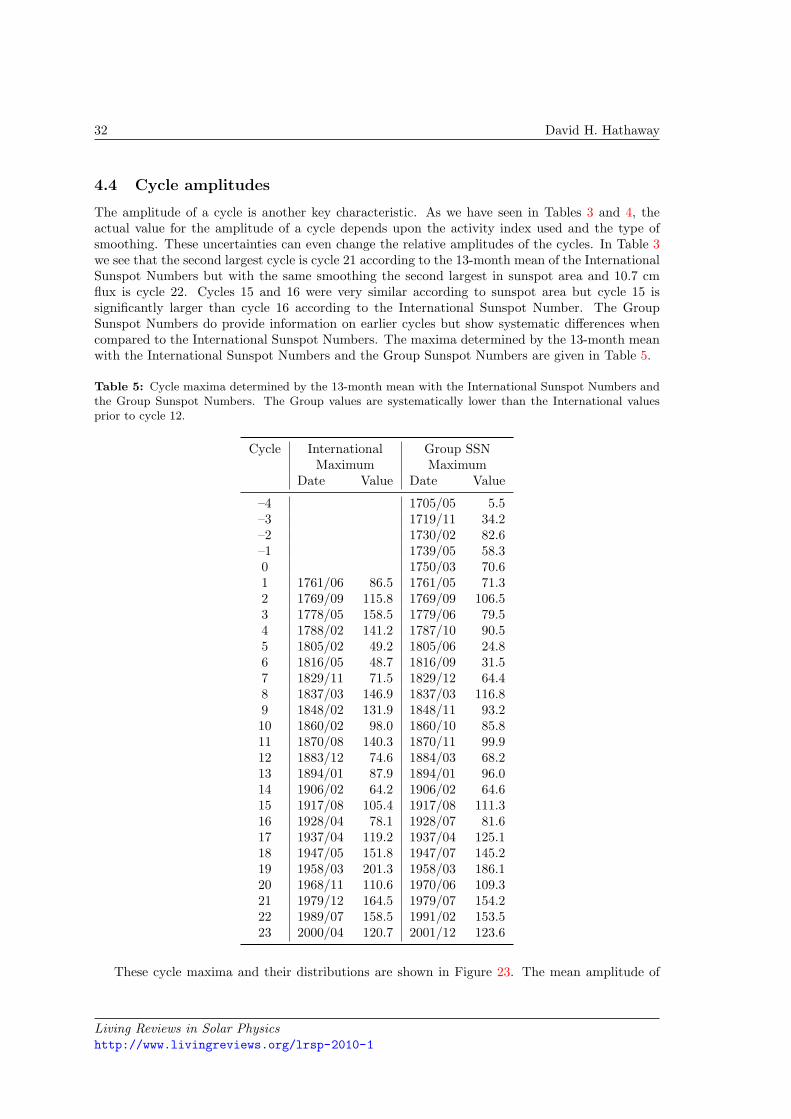
The amplitude of a cycle is another key characteristic. As we have seen in Tables 3 and 4, theactual value for the amplitude of a cycle depends upon the activity index used and the type ofsmoothing. These uncertainties can even change the relative amplitudes of the cycles. In Table 3we see that the second largest cycle is cycle 21 according to the 13-month mean of the InternationalSunspot Numbers but with the same smoothing the second largest in sunspot area and 10.7 cmflux is cycle 22. Cycles 15 and 16 were very similar according to sunspot area but cycle 15 issignificantly larger than cycle 16 according to the International Sunspot Number. The GroupSunspot Numbers do provide information on earlier cycles but show systematic differences whencompared to the International Sunspot Numbers. The maxima determined by the 13-month meanwith the International Sunspot Numbers and the Group Sunspot Numbers are given in Table 5.
Table 5: Cycle maxima determined by the 13-month mean with the International Sunspot Numbers andthe Group Sunspot Numbers. The Group values are systematically lower than the International valuesprior to cycle 12.
Cycle InternationalMaximum
Group SSNMaximum
Date Value Date Value
–4 1705/05 5.5–3 1719/11 34.2–2 1730/02 82.6–1 1739/05 58.30 1750/03 70.61 1761/06 86.5 1761/05 71.32 1769/09 115.8 1769/09 106.53 1778/05 158.5 1779/06 79.54 1788/02 141.2 1787/10 90.55 1805/02 49.2 1805/06 24.86 1816/05 48.7 1816/09 31.57 1829/11 71.5 1829/12 64.48 1837/03 146.9 1837/03 116.89 1848/02 131.9 1848/11 93.210 1860/02 98.0 1860/10 85.811 1870/08 140.3 1870/11 99.912 1883/12 74.6 1884/03 68.213 1894/01 87.9 1894/01 96.014 1906/02 64.2 1906/02 64.615 1917/08 105.4 1917/08 111.316 1928/04 78.1 1928/07 81.617 1937/04 119.2 1937/04 125.118 1947/05 151.8 1947/07 145.219 1958/03 201.3 1958/03 186.120 1968/11 110.6 1970/06 109.321 1979/12 164.5 1979/07 154.222 1989/07 158.5 1991/02 153.523 2000/04 120.7 2001/12 123.6
These cycle maxima and their distributions are shown in Figure 23. The mean amplitude of
Living Reviews in Solar Physicshttp://www.livingreviews.org/lrsp-2010-1

The Solar Cycle 33
cycles 1 to 23 from the International Sunspot Numbers is 114 with a standard deviation of 40.The mean amplitude of Cycles –4 to 23 from the Group Sunspot Numbers is 90 with a standarddeviation of 41.
-5 0 5 10 15 20 0 5 10 Cycle Number Number of Cycles
0
40
80
120
160
200
Am
pli
tud
e (
Su
ns
po
t N
um
be
r)
Figure 23: The left panel shows cycle amplitudes as functions of cycle number. The filled circles show the13-month mean maxima with the Group Sunspot Numbers while the open circles show the maxima withthe International Sunspot Numbers. The right panel shows the cycle amplitude distributions (solid linesfor the Group values, dotted lines for the International values). The Group amplitudes are systematicallylower than the International amplitudes for cycles prior to cycle 12 and have a nearly normal distribution.The amplitudes for the International Sunspot Number are skewed toward higher values.
4.5 Cycle shape
Sunspot cycles are asymmetric with respect to their maxima (Waldmeier, 1935). The elapsed timefrom minimum up to maximum is almost always shorter than the elapsed time from maximumdown to minimum. An average cycle can be constructed by stretching and contracting each cycleto the average length, normalizing each to the average amplitude, and then taking the average ateach month. This is shown in Figure 24 for cycles 1 to 22. The average cycle takes about 48 monthsto rise from minimum up to maximum and about 84 months to fall back to minimum again.
Various functions have been used to fit the shape of the cycle and/or its various phases. Stewartand Panofsky (1938) proposed a single function for the full cycle that was the product of a powerlaw for the initial rise and an exponential for the decline. They found the four parameters (startingtime, amplitude, exponent for the rise, and time constant for the decline) that give the best fit foreach cycle. Nordemann (1992) fit both the rise and the decay with exponentials that each requiredthree parameters – an amplitude, a time constant, and a starting time. Elling and Schwentek(1992) also fit the full cycle but with a modified 𝐹 -distribution density function which requires fiveparameters. Hathaway et al. (1994) suggested yet another function – similar to that of Stewart andPanofsky (1938) but with a fixed (cubic) power law and a Gaussian for the decline. This functionof time
𝐹 (𝑡) = 𝐴
(𝑡− 𝑡0
𝑏
)3[exp
(𝑡− 𝑡0
𝑏
)2
− 𝑐
]−1
(6)
has four parameters: an amplitude 𝐴, a starting time 𝑡0, a rise time 𝑏, and an asymmetry parameter𝑐. The average cycle is well fit with 𝐴 = 193, 𝑏 = 54, 𝑐 = 0.8, and 𝑡0 = 4 months prior to minimum.
Living Reviews in Solar Physicshttp://www.livingreviews.org/lrsp-2010-1

34 David H. Hathaway
0 12 24 36 48 60 72 84 96 108 120 132Time (months)
0
25
50
75
100
125
Su
nsp
ot
Nu
mb
er
Figure 24: The average of cycles 1 to 22 (thick line) normalized to the average amplitude and period.The average cycle is asymmetric in time with a rise to maximum over 4 years and a fall back to minimumover 7 years. The 22 individual, normalized cycles are shown with the thin lines.
This fit to the average cycle is shown in Figure 25. Hathaway et al. (1994) found that good fitsto most cycles could be obtained with a fixed value for the parameter 𝑐 and a parameter 𝑏 that isallowed to vary with the amplitude – leaving a function of just two parameters – amplitude andstarting time.
4.6 Rise time vs. amplitude (The Waldmeier Effect)
A number of relationships have been found between various sunspot cycle characteristics. Amongthe more significant relationships is the Waldmeier Effect (Waldmeier, 1935, 1939) in which thetime it takes for the sunspot number to rise from minimum to maximum is inversely proportionalto the cycle amplitude. This is shown in Figure 26 for both the International Sunspot Numberand the 10.7 cm radio flux data. Times and values for the maxima are taken from the 24-monthGaussian given in Table 4. Times for the minima are taken from the average dates given in Table 2.Both of these indices exhibit the Waldmeier Effect but with the 10.7 cm flux maxima delayed byabout 6 months. This is larger than, but consistent with the delays seen by Bachmann and White(1994). The best fit through the Sunspot Number data gives
Rise Time (in months) ≈ 35 + 1800/Amplitude (in Sunspot Number). (7)
While this effect is widely quoted and accepted it does face a number of problems. Hathawayet al. (2002) found that the effect was greatly diminished when Group Sunspot Numbers were used(the anti-correlation between rise time and amplitude dropped from –0.7 to –0.34). Inspection ofFigure 26 clearly shows significant scatter. Dikpati et al. (2008b) noted that the effect is not seen forsunspot area data. This is consistent with the date in Tables 3 and 4 which show that significantlydifferent dates for maxima are found with sunspot area when compared to sunspot number. Thedates can differ by more than a year but without any evidence of systematic differences (areasometimes leads number and other times lags).
Living Reviews in Solar Physicshttp://www.livingreviews.org/lrsp-2010-1

The Solar Cycle 35
0 12 24 36 48 60 72 84 96 108 120 132Time (months)
0
25
50
75
100
125S
un
sp
ot
Nu
mb
er
Figure 25: The average cycle (solid line) and the Hathaway et al. (1994) functional fit to it (dotted line)from Equation (6). This fit has the average cycle starting 4 months prior to minimum, rising to maximumover the next 54 months, and continuing about 18 months into the next cycle.
50 100 150 200Cycle Amplitude (SSN)
30
40
50
60
70
80
Cycle
Ris
e T
ime (
mo
nth
s)
Figure 26: The Waldmeier Effect. The cycle rise time (from minimum to maximum) plotted versus cycleamplitude for International Sunspot Number data from cycles 1 to 23 (filled dots) and for 10.7 cm RadioFlux data from cycles 19 to 23 (open circles). This gives an inverse relationship between amplitude andrise time shown by the solid line for the Sunspot Number data and with the dashed line for the RadioFlux data. The Radio Flux maxima are systematically later than the Sunspot number data as also seenin Table 4.
Living Reviews in Solar Physicshttp://www.livingreviews.org/lrsp-2010-1
36 David H. Hathaway
4.7 Period vs. amplitude
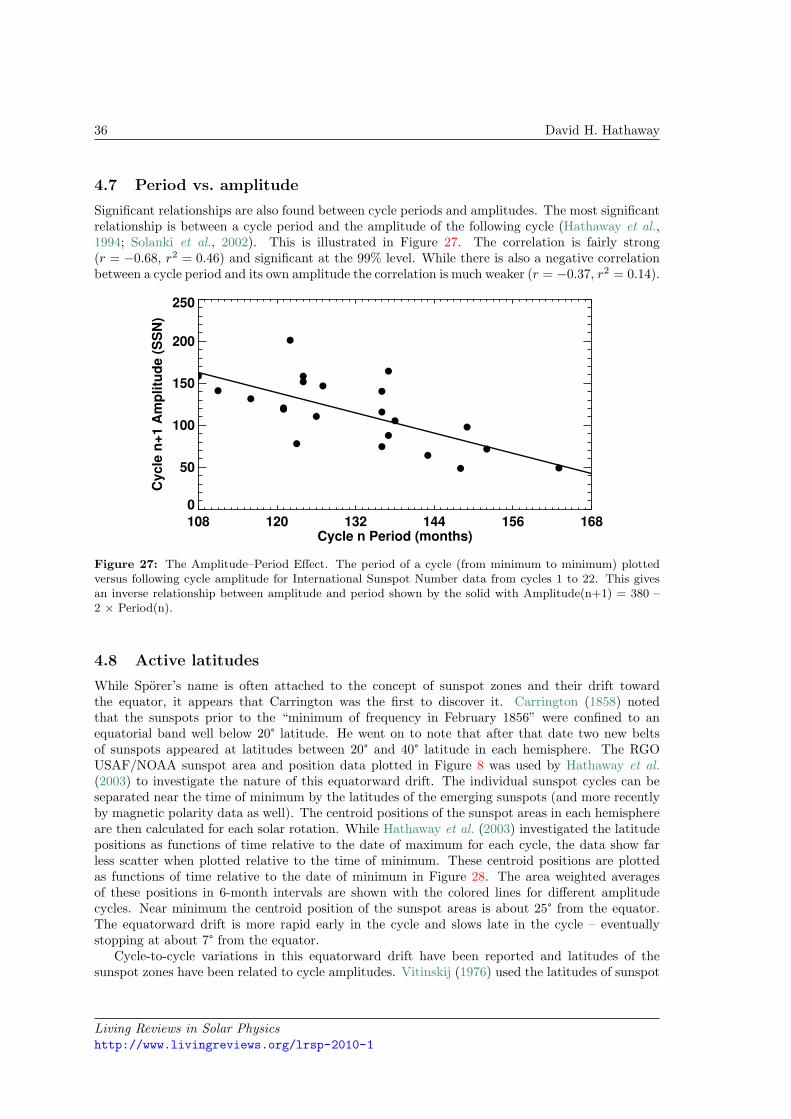
Significant relationships are also found between cycle periods and amplitudes. The most significantrelationship is between a cycle period and the amplitude of the following cycle (Hathaway et al.,1994; Solanki et al., 2002). This is illustrated in Figure 27. The correlation is fairly strong(𝑟 = −0.68, 𝑟2 = 0.46) and significant at the 99% level. While there is also a negative correlationbetween a cycle period and its own amplitude the correlation is much weaker (𝑟 = −0.37, 𝑟2 = 0.14).
108 120 132 144 156 168Cycle n Period (months)
0
50
100
150
200
250
Cycle
n+
1 A
mp
litu
de (
SS
N)
Figure 27: The Amplitude–Period Effect. The period of a cycle (from minimum to minimum) plottedversus following cycle amplitude for International Sunspot Number data from cycles 1 to 22. This givesan inverse relationship between amplitude and period shown by the solid with Amplitude(n+1) = 380 –2 × Period(n).
4.8 Active latitudes
While Sporer’s name is often attached to the concept of sunspot zones and their drift towardthe equator, it appears that Carrington was the first to discover it. Carrington (1858) notedthat the sunspots prior to the “minimum of frequency in February 1856” were confined to anequatorial band well below 20° latitude. He went on to note that after that date two new beltsof sunspots appeared at latitudes between 20° and 40° latitude in each hemisphere. The RGOUSAF/NOAA sunspot area and position data plotted in Figure 8 was used by Hathaway et al.(2003) to investigate the nature of this equatorward drift. The individual sunspot cycles can beseparated near the time of minimum by the latitudes of the emerging sunspots (and more recentlyby magnetic polarity data as well). The centroid positions of the sunspot areas in each hemisphereare then calculated for each solar rotation. While Hathaway et al. (2003) investigated the latitudepositions as functions of time relative to the date of maximum for each cycle, the data show farless scatter when plotted relative to the time of minimum. These centroid positions are plottedas functions of time relative to the date of minimum in Figure 28. The area weighted averagesof these positions in 6-month intervals are shown with the colored lines for different amplitudecycles. Near minimum the centroid position of the sunspot areas is about 25° from the equator.The equatorward drift is more rapid early in the cycle and slows late in the cycle – eventuallystopping at about 7° from the equator.
Cycle-to-cycle variations in this equatorward drift have been reported and latitudes of thesunspot zones have been related to cycle amplitudes. Vitinskij (1976) used the latitudes of sunspot
Living Reviews in Solar Physicshttp://www.livingreviews.org/lrsp-2010-1

The Solar Cycle 37
0 2 4 6 8 10 12Time (Years from Min)
0
10
20
30
40L
ati
tud
e (
Deg
rees)
Area > 1000 µHem
Area > 500 µHem
Area > 20 µHem
Large Cycles
Medium Cycles
Small Cycles
Figure 28: Latitude positions of the sunspot area centroid in each hemisphere for each CarringtonRotation as functions of time from cycle minimum. Three symbol sizes are used to differentiate dataaccording to the daily average of the sunspot area for each hemisphere and rotation. The centroids of thecentroids in 6-month intervals are shown with the red line for large amplitude cycles, with the green linefor medium amplitude cycles, and with the blue line for the small amplitude cycles.
near minimum as a predictor for the amplitude of cycle 21. Separating the cycles according to sizenow suggests that this is a poor indicator of cycle amplitude. Regardless of amplitude class allcycles start with sunspot zones centered at about 25°. This is illustrated in Figure 28 where thelatitude positions of the sunspot area centroids are shown for small amplitude cycles (cycles 12,13, 14, and 16) in blue, for medium amplitude cycles (cycles 15, 17, 20, and 23) in green, and forlarge amplitude cycles (cycles 18, 19, 21, and 22) in red.
Becker (1954) and Waldmeier (1955) noted that in large cycles, the latitudes of the sunspotzones are higher at maximum than in small cycles. This is indicated in the data plotted inFigure 28. The sunspot zones in large amplitude cycles tend to stay at higher latitudes than inmedium or small cycles from about a year after minimum to about five years after minimum. Sincelarge amplitude cycles reach their maxima sooner than do medium or small amplitude cycles (theWaldmeier Effect – Section 4.6), the latitude differences are increased further.
The latitudinal width of the sunspot zones also varies over the cycle and as a function of cycleamplitude. This is illustrated in Figure 29 where the latitudinal widths of the sunspot zones areplotted for each hemisphere and Carrington rotation. The active latitude bands are narrow atminimum, expand to a maximum width at about the time of maximum, and then narrow againduring the declining phase of the cycle. Larger cycles achieve greater widths than do smallercycles. At all cycle phases and for all cycle amplitudes the active latitudes are fairly symmetricallycentered with no systematic skew in the latitude distribution of sunspot areas.
4.9 Active hemispheres
Comparisons of the activity in each solar hemisphere show significant asymmetries. Spoerer (1889)and Maunder (1890, 1904) noted that there were often long periods of time when most of thesunspots were found preferentially in one hemisphere and not the other. Waldmeier (1971) foundthat this asymmetry extended to other measures of activity including faculae, prominences, andcoronal brightness. Roy (1977) reported that major flares and magnetically complex sunspot
Living Reviews in Solar Physicshttp://www.livingreviews.org/lrsp-2010-1

38 David H. Hathaway
0 2 4 6 8 10 12Time (Years from Min)
0
5
10
15
Su
nsp
ot
Zo
ne W
idth
(D
eg
rees)
Area > 1000 µHem
Area > 500 µHem
Area > 20 µHem
Large Cycles
Medium Cycles
Small Cycles
Figure 29: Latitudinal widths of the sunspot area centroid in each hemisphere for each CarringtonRotation as functions of time from cycle minimum. Three symbol sizes are used to differentiate dataaccording to the daily average of the sunspot area for each hemisphere and rotation. The centroids of thecentroids in 6-month intervals are shown with the red line for large amplitude cycles, with the green linefor medium amplitude cycles, and with the blue line for the small amplitude cycles.
groups also showed strong north–south asymmetry. Simply quantifying the asymmetry itself isproblematic. Taking the difference between hemispheric measures of activity (absolute asymmetry)produces strong signals around the times of maxima while taking the ratio of the difference to thesum (relative asymmetry) produces strong signals around the times of minima. Figure 30 showsthe absolute asymmetry (North – South) of several key indicators. It is clear from this figure thathemispheric asymmetry is real (it consistently appears in all four indicators) and is often persistent– lasting for many years at a time. The absolute asymmetry in the RGO USAF/NOAA sunspotarea smoothed with the 24-month Gaussian filter given by Equation (4) is shown in Figure 31.This indicates that north–south asymmetry can persist for years.
Systematic variations over the course of a solar cycle or as a function of cycle amplitude havebeen suggested but these variations have invariably been found to change from cycle to cycle(See Section 5). For example, Newton and Milsom (1955) showed that the northern hemispheredominated in the early phases of cycles 12 – 15 with a switch to dominance in the south later ineach cycle while the opposite was true for cycles 17 – 18. (This can be seen in Figure 31 wherecycle 12 is the first cycle shown.) Waldmeier (1957, 1971) noted that a significant part of thesevariations can be accounted for by the fact that the two hemispheres are not exactly in phase.When the northern hemisphere activity leads that in the southern hemisphere, the north willdominate early in the cycle while the south will dominate in the declining phase. Carbonell et al.(1993) examined the relative asymmetry in sunspot areas with a variety of statistical tools andconcluded that the signal is dominated by a random (and intermittent) component but contains acomponent that varies over a cycle and a component that gives long-term trends. The variationin the strength of the asymmetry over the course of an average cycle is strongly dependent uponhow the asymmetry is quantified (strong at minimum for relative asymmetry, strong at maximumfor absolute asymmetry). The variation from cycle-to-cycle will be discussed in Section 5.
Living Reviews in Solar Physicshttp://www.livingreviews.org/lrsp-2010-1

The Solar Cycle 39
1975 1980 1985 1990 1995 2000Date
-2000
-1000
0
1000
2000
As
ym
me
try
(N
ort
h -
So
uth
)
Sunspot AreaFlare Index • 146Sunspot Groups • 443Magnetic Index • 234
Figure 30: Absolute north–south asymmetry (North – South) in four different activity indicators. Sunspotarea is plotted in black. The Flare Index scaled by 146 is shown in red. The number of sunspot groupsscaled by 443 is shown in green. The Magnetic Index scaled by 234 is plotted in blue.
1880 1900 1920 1940 1960 1980 2000Date
-500
0
500
1000
Su
nsp
ot
Are
a (
µH
em
)
(North - South)
(North + South)/10
Figure 31: Smoothed north–south asymmetry in sunspot area. The hemispheric difference is shown withthe solid line while the total area scaled by 1/10 is shown with the dotted line.
Living Reviews in Solar Physicshttp://www.livingreviews.org/lrsp-2010-1
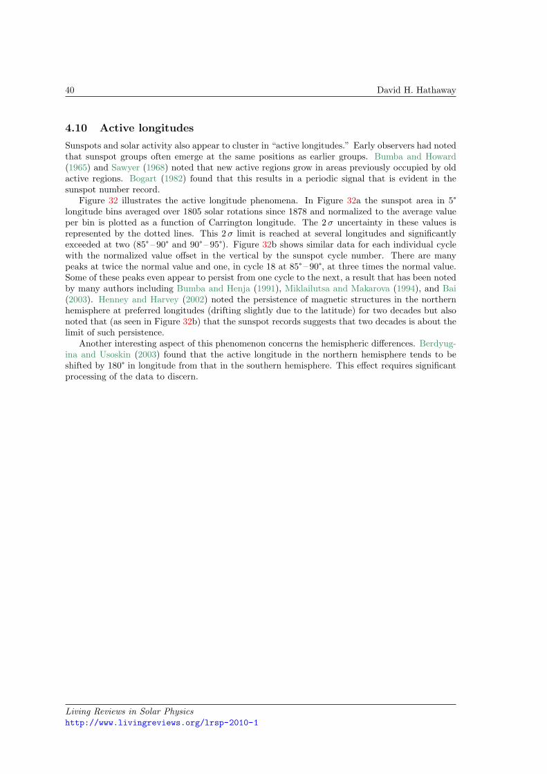
40 David H. Hathaway
4.10 Active longitudes
Sunspots and solar activity also appear to cluster in “active longitudes.” Early observers had notedthat sunspot groups often emerge at the same positions as earlier groups. Bumba and Howard(1965) and Sawyer (1968) noted that new active regions grow in areas previously occupied by oldactive regions. Bogart (1982) found that this results in a periodic signal that is evident in thesunspot number record.
Figure 32 illustrates the active longitude phenomena. In Figure 32a the sunspot area in 5°longitude bins averaged over 1805 solar rotations since 1878 and normalized to the average valueper bin is plotted as a function of Carrington longitude. The 2 𝜎 uncertainty in these values isrepresented by the dotted lines. This 2 𝜎 limit is reached at several longitudes and significantlyexceeded at two (85° – 90° and 90° – 95°). Figure 32b shows similar data for each individual cyclewith the normalized value offset in the vertical by the sunspot cycle number. There are manypeaks at twice the normal value and one, in cycle 18 at 85° – 90°, at three times the normal value.Some of these peaks even appear to persist from one cycle to the next, a result that has been notedby many authors including Bumba and Henja (1991), Miklailutsa and Makarova (1994), and Bai(2003). Henney and Harvey (2002) noted the persistence of magnetic structures in the northernhemisphere at preferred longitudes (drifting slightly due to the latitude) for two decades but alsonoted that (as seen in Figure 32b) that the sunspot records suggests that two decades is about thelimit of such persistence.
Another interesting aspect of this phenomenon concerns the hemispheric differences. Berdyug-ina and Usoskin (2003) found that the active longitude in the northern hemisphere tends to beshifted by 180° in longitude from that in the southern hemisphere. This effect requires significantprocessing of the data to discern.
Living Reviews in Solar Physicshttp://www.livingreviews.org/lrsp-2010-1

The Solar Cycle 41
0 30 60 90 120 150 180 210 240 270 300 330 360Longitude
0.6
0.8
1.0
1.2
1.4
Rela
tive A
rea
a
0 30 60 90 120 150 180 210 240 270 300 330 360Longitude
1012
14
16
18
20
22
24
Rela
tive A
rea
b
Figure 32: Active longitudes in sunspot area. The normalized sunspot area in 5° longitude bins is plottedin the upper panel (a) for the years 1878 – 2009. The dotted lines represent two standard errors in thenormalized values. The sunspot area in several longitude bins meets or exceeds these limits. The individualcycles (12 through 23) are shown in the lower panel (b) with the normalized values offset in the verticalby the cycle number. Some active longitudes appear to persist from cycle to cycle.
Living Reviews in Solar Physicshttp://www.livingreviews.org/lrsp-2010-1

42 David H. Hathaway
5 Long-Term Variability
Systematic variations from cycle-to-cycle and over many cycles could be significant discriminatorsin models of the solar cycle and might aid in predicting future cycles. Several key aspects of long-term variability have been noted: a 70-year period of extremely low activity from 1645 to 1715 (theMaunder Minimum); a gradual increase in cycle amplitudes since the Maunder Minimum (a SecularTrend); an 80 – 90 year variation in cycle amplitudes (the Gleissberg Cycle); a two-cycle variationwith odd numbered cycles higher than the preceding even numbered cycles (the Gnevyshev–OhlEffect); a 205-year cycle in radio isotope proxies (the Suess Cycle); and other long term variationsseen in radio isotopes. These aspects of long-term variability are examined in this section.
5.1 The Maunder Minimum
Maunder (1890) reporting on the work of Sporer noted that for a seventy year period from 1645 –1715 the course of the sunspot cycle was interrupted. Eddy (1976) provided additional referencesto the lack of activity during this period and referred to it as the Maunder Minimum. He notedthat many observers prior to 1890 had noticed this lack of activity and that both he and Maunderwere simply pointing out an overlooked aspect of solar activity.
Hoyt and Schatten (1998) compiled observations from numerous sources to provide nearlycomplete coverage of sunspot observations during the period of the Maunder Minimum. Theseobservations (Figure 33) clearly show the lack of activity and apparent cessation of the sunspotcycle during the Maunder Minimum. Nonetheless, Beer et al. (1998) find evidence for a weak cyclicvariation in 10Be during the Maunder Minimum suggesting that the magnetic cycle was still inprogress but too weak to produce the intense magnetic fields in sunspots. In addition, Ribes andNesme-Ribes (1993) found that the sunspot that were observed in the latter half of the MaunderMinimum were at low latitudes and dominant in the southern hemisphere – another indication ofweak/marginal magnetic fields.
1600 1700 1800 1900 2000Date
0
50
100
150
200
Su
ns
po
t N
um
be
r
MaunderMinimum
Figure 33: The Maunder Minimum. The yearly averages of the daily Group Sunspot Numbers are plottedas a function of time. The Maunder Minimum (1645 – 1715) is well observed in this dataset.
5.2 The secular trend
Since the Maunder Minimum there seems to have been a steady increase in sunspot cycle amplitudes(Wilson, 1988). This is readily seen in the yearly Group Sunspot Numbers plotted in Figure 33 andin the cycle amplitudes for Group Sunspot Numbers plotted in Figure 23. Hathaway et al. (2002)found a correlation coefficient of 0.7 between cycle amplitude and cycle number. This linear trendis not so apparent in the International Sunspot numbers plotted in Figure 23. It obviously cannot
Living Reviews in Solar Physicshttp://www.livingreviews.org/lrsp-2010-1

The Solar Cycle 43
continue forever but may represent an important characteristic of the solar cycle that should berepresented in viable models for the cycle. Radioisotopes also show this recent trend (Solanki et al.,2004) and indicate many upward and downward trends over the last 11,000 years.
5.3 The Gleissberg Cycle
Numerous authors have noted multi-cycle periodicities in the sunspot cycle amplitudes. Gleissberg(1939) noted a periodicity of seven or eight cycles in cycle amplitudes from 1750 to 1928. WhileGarcia and Mouradian (1998) suggest that a third period of this cycle can be found in the sunspotdata, others (Hathaway et al., 1999) suggest that the period is changing or (Rozelot, 1994; Ogurtsovet al., 2002) that it consists of two different components (one with a 90 – 100 year period and asecond with a 50 – 60 year period). A simple sinusoid fit to the residual cycle amplitudes when thesecular trend is removed now gives a 9.1 cycle periodicity. This best fit is shown in Figure 34.
0 5 10 15 20 25Cycle Number n
0
50
100
150
200
250
Rm
ax
(n)
(SS
N)
Figure 34: The Gleissberg Cycle. The best fit of cycle amplitudes to a simple sinusoidal function of cyclenumber is shown by the solid line (which includes the secular trend).
5.4 Gnevyshev–Ohl Rule (Even–Odd Effect)
Gnevyshev and Ohl (1948) found that if solar cycles are arranged in pairs with an even numberedcycle and the following odd numbered cycle then the sum of the sunspot numbers in the odd cycle ishigher than in the even cycle. This is referred to as the Gnevyshev–Ohl Rule or Even–Odd Effect.This Rule is illustrated in Figure 35. With the exception of the Cycle 4/5 pair, this relationshipheld until cycle 23 showed that the cycle 22/23 pair was also an exception. If cycle amplitudes arecompared then the Cycle 8/9 pair is also an exception. This rule also holds for other indicators ofcycle amplitude such as sunspot area. While much has been said about this rule relative to the22-year Hale cycle, it is difficult to understand why the order (even-odd vs. odd-even) of the pairingshould make a difference. The observed effect does however impact flux transport models for thesurface fields (see Sheeley Jr, 2005, for a review). Since the odd cycles all have the same magneticpolarity, stronger odd cycles will tend to build up polar fields of one polarity to the extent thatthe transport during the even cycles cannot reverse the polar fields without associated changes intransport.
Living Reviews in Solar Physicshttp://www.livingreviews.org/lrsp-2010-1
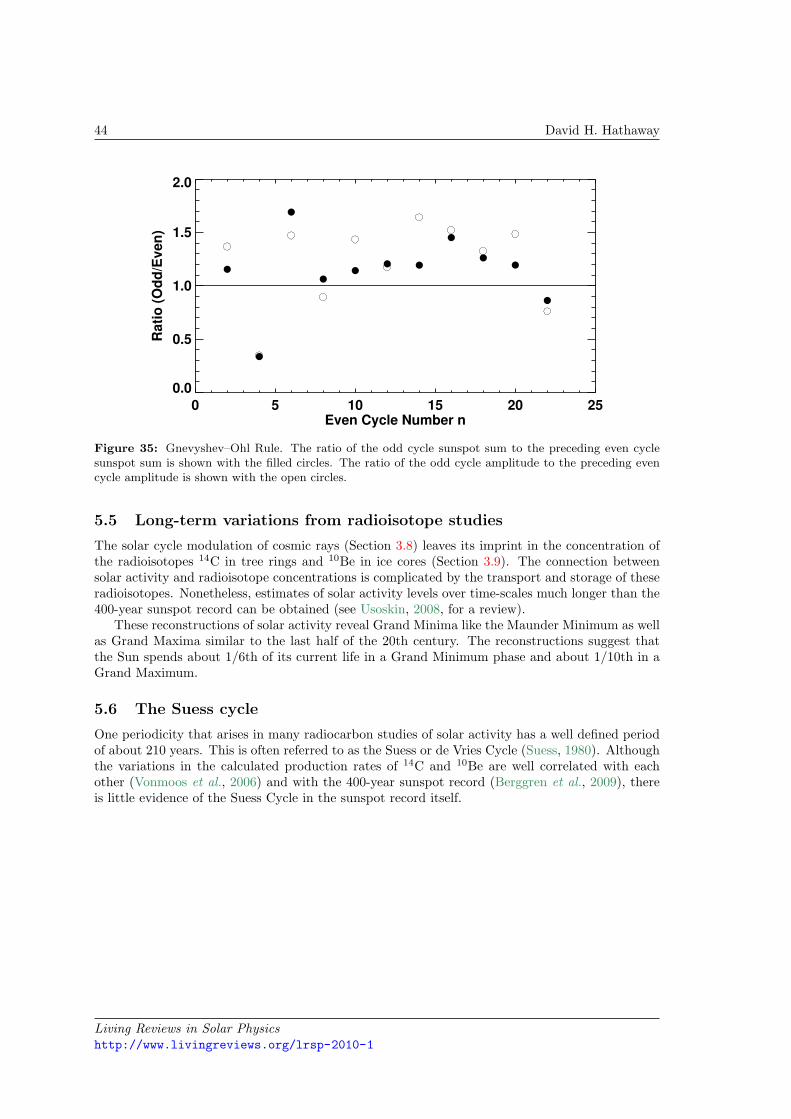
44 David H. Hathaway
0 5 10 15 20 25Even Cycle Number n
0.0
0.5
1.0
1.5
2.0
Ra
tio
(O
dd
/Ev
en
)
Figure 35: Gnevyshev–Ohl Rule. The ratio of the odd cycle sunspot sum to the preceding even cyclesunspot sum is shown with the filled circles. The ratio of the odd cycle amplitude to the preceding evencycle amplitude is shown with the open circles.
5.5 Long-term variations from radioisotope studies
The solar cycle modulation of cosmic rays (Section 3.8) leaves its imprint in the concentration ofthe radioisotopes 14C in tree rings and 10Be in ice cores (Section 3.9). The connection betweensolar activity and radioisotope concentrations is complicated by the transport and storage of theseradioisotopes. Nonetheless, estimates of solar activity levels over time-scales much longer than the400-year sunspot record can be obtained (see Usoskin, 2008, for a review).
These reconstructions of solar activity reveal Grand Minima like the Maunder Minimum as wellas Grand Maxima similar to the last half of the 20th century. The reconstructions suggest thatthe Sun spends about 1/6th of its current life in a Grand Minimum phase and about 1/10th in aGrand Maximum.
5.6 The Suess cycle
One periodicity that arises in many radiocarbon studies of solar activity has a well defined periodof about 210 years. This is often referred to as the Suess or de Vries Cycle (Suess, 1980). Althoughthe variations in the calculated production rates of 14C and 10Be are well correlated with eachother (Vonmoos et al., 2006) and with the 400-year sunspot record (Berggren et al., 2009), thereis little evidence of the Suess Cycle in the sunspot record itself.
Living Reviews in Solar Physicshttp://www.livingreviews.org/lrsp-2010-1

The Solar Cycle 45
6 Short-Term Variability
There are significant variations in solar activity on time scales shorter than the sunspot cycle.This is evident when the sunspot number record is filtered to remove both solar rotation effects(periods of about 27-days and less) and solar cycle effects. This signal is shown in Figure 36for the years 1850 – 2000. In this figure the daily sunspot numbers are filtered with a taperedGaussian shaped filter (Equation (4)) with a FWHM of 54 days. This reduces all signals withperiods shorter than 54-days to less than 2% of their original amplitude. The resulting signal issampled at 27-day intervals and then filtered again with a similar Gaussian with a FWHM of 24rotations. The lower panel of Figure 36 shows this final signal for the time period while the upperpanel shows the residual obtained when this smoothed sunspot number signal is subtracted from54-day filtered data. This residual signal is quite chaotic but shows some interesting behavior andquasi-periodicities.
1850 1900 1950 2000
Date
-50
-25
0
25
50
Re
sid
ua
l S
SN
1850 1900 1950 2000
Date
0
50
100
150
200
Sm
oo
the
d S
SN
Figure 36: Short-term variations. The lower panel shows the daily International Sunspot Number (SSN)smoothed with a 24-rotation FWHM Gaussian. The upper panel shows the residual SSN signal smoothedwith a 54-day Gaussian and sampled at 27-day intervals.
6.1 154-day periodicity
A 154 day periodic signal was noted in gamma-ray flare activity seen from SMM by Rieger et al.(1984) for the time interval from 1980/02 to 1983/08. This signal was also found by Bai and Cliver(1990) in proton flares for both this interval and an earlier interval from 1958/01 to 1971/12.Ballester et al. (2002) found that this signal was also seen in the Mt. Wilson sunspot index forthe 1980 – 1983 time frame. Lean (1990) analyzed the signal in the sunspot area data and found
Living Reviews in Solar Physicshttp://www.livingreviews.org/lrsp-2010-1

46 David H. Hathaway
that it occurs in episodes around the epochs of sunspot cycle maxima and that its frequency driftsas well. A wavelet transform of the bandpass-limited (54 days . period . 2 years) daily sunspotnumbers shown in the upper panel of Figure 36 is shown in Figure 37 with a horizontal red lineindicating periods of 154 days. The strong signal in the early 1980s as well as other intermittentintervals is clearly evident in this plot.
1850 1900 1950 2000Date
10.0
1.0
0.1
Pe
rio
d (
ye
ars
)
Figure 37: Morlet wavelet transform spectrum of the bandpass-limited daily International Sunspot Num-ber. Increasing wavelet power is represented by colors from black through blue, green, and yellow to red.The Cone-Of-Influence is shown with the white curves. Periods of 154-days are indicated by the horizontalred line.
6.2 Quasi-biennial variations and double peaked maxima
Another interesting periodicity is one found with a period of about two years (Benevolenskaya, 1995;Mursula et al., 2003). Many sunspot cycles exhibit double peaks when the monthly InternationalSunspot Number is smoothed with the traditional 13-month running mean. This was noted byGnevyshev (1963, 1967, 1977) and often referred to as the Gnevyshev Gap. Wang and Sheeley Jr(2003) found that the Sun’s dipole magnetic moment and open magnetic flux exhibits multiplepeaks with quasi-periodicities of about 1.3 years that they attributed to the stochastic processesof active region emergence and a decay time of about 1 year set by the dynamical processes ofdifferential rotation, meridional flow, and supergranule diffusion. These quasi-periodic variationsare also evident in the wavelet spectrum shown in Figure 37. Multiple significant peaks of powerare seen intermittently at periods between 1 and 2 years and are most prevalent near the time ofcycle maxima (Bazilevskaya et al., 2000). A signal with a similar period is seen in the TachoclineOscillations – periodic variations in the shear at the base of the convection zone (Howe et al.,2000). These tachocline oscillations have also been found to be intermittent (Howe et al., 2007).
Living Reviews in Solar Physicshttp://www.livingreviews.org/lrsp-2010-1

The Solar Cycle 47
7 Solar Cycle Predictions
Predicting the solar cycle is indeed very difficult. A cursory examination of the sunspot recordreveals a wide range of cycle amplitudes (Figure 2). Over the last 24 cycles the average amplitude(in terms of the 13-month-smoothed monthly averages of the daily sunspot number) was about114. Over the last 400 years the cycle amplitudes have varied widely – from basically zero throughthe Maunder Minimum to the two small cycles of the Dalton Minimum at the start of the 19thcentury (amplitudes of 49.2 and 48.7) to the recent string of large cycles (amplitudes of 151.8,201.3, 110.6, 164.5, 158.5, and 120.8). In addition to the changes in the amplitude of the cycle,there are changes in cycle length and cycle shape as discussed in Section 4.
7.1 Predicting an ongoing cycle
One popular and often used method for predicting solar activity was first described by McNishand Lincoln (1949). As a cycle progresses the smoothed monthly sunspot numbers are comparedto the average cycle for the same number of months since minimum. The difference between thetwo is used to project future differences between predicted and mean cycle. The McNish–Lincolnregression technique originally used yearly values and only projected one year into the future.Later improvements to the technique use monthly values and use an auto-regression to predict theremainder of the cycle.
One problem with the modified McNish–Lincoln technique is that it does not account forsystematic changes in the shape of the cycle with cycle amplitude (i.e. the Waldmeier Effect,Section 4.6). Another problem with the McNish–Lincoln method is its sensitivity to choices forthe date of cycle minimum. Both the systematic changes in shape and the sensitivity to cycleminimum choice can be accounted for with techniques that fit the monthly data to parametriccurves (e.g. Stewart and Panofsky, 1938; Elling and Schwentek, 1992; Hathaway et al., 1994).The two-parameter function of Hathaway et al. (1994) (Equation (6)) closely mimics the changingshape of the sunspot cycle. Prediction requires fitting the data to the function with a best fit foran initial starting time, 𝑡0, and amplitude, 𝐴.
Both the Modified McNish–Lincoln and the curve-fitting techniques work nicely once a sunspotcycle is well under way. The critical point seems to be 2 – 3 years after minimum near the time ofthe inflection point on the rise to maximum. Predictions for cycles 22 and 23 using the ModifiedMcNish–Lincoln and the Hathaway, Wilson, and Reichmann curve-fitting techniques 24 monthsafter minimum are shown in Figure 38. Since cycle 23 had an amplitude very close to the average ofcycles 10 – 22, both of these predictions are very similar. Distinct differences are seen for larger orsmaller cycles and when different dates are taken for minimum with the McNish–Lincoln method.
Predicting the size and timing of a cycle prior to its start (or even during the first year ortwo of the cycle) requires methods other than auto-regression or curve-fitting. There is a long,and growing, list of measured quantities that can and have been used to predict future cycleamplitudes. Prediction methods range from simple climatological means to physics-based dynamoswith assimilated data.
7.2 Predicting future cycle amplitudes based on cycle statistics
The mean amplitude of the last 𝑛 cycles gives the benchmark for other prediction techniques. Themean of the last 23 cycle amplitudes is 114.1 ± 40.4 where the error is the standard deviationabout the mean. This represents a prediction without any skill. If other methods cannot predictwith significantly better accuracy they have little use.
One class of prediction techniques is based on trends and periodicities in the cycle amplitudes.In general there has been an upward trend in cycle amplitudes since the Maunder Minimum.
Living Reviews in Solar Physicshttp://www.livingreviews.org/lrsp-2010-1

48 David H. Hathaway
0 20 40 60 80 100 120Time (months from Minimum)
0
50
100
150
200
250
Cy
cle
22
Su
ns
po
t N
um
be
r
Observed
M-M-L
H-W-R
0 20 40 60 80 100 120Time (months)
0
50
100
150
200
250
Cy
cle
23
Su
ns
po
t N
um
be
r
Observed
M-M-L
H-W-R
Figure 38: Predictions for cycles 22 and 23 using the Modified McNish–Lincoln (M-M-L) auto-regressiontechnique and the Hathaway, Wilson, and Reichmann (H-W-R) curve-fitting technique 24 months afterthe minima for each cycle.
Projecting this trend to the next cycle gives a prediction slightly better than the mean. A number ofperiodicities have been noted in the cycle amplitude record. Gleissberg (1939) noted a long-periodvariation in cycle amplitudes with a period of seven or eight cycles (Section 5.3 and Figure 34).Gnevyshev and Ohl (1948) noted a two-cycle periodicity with the odd numbered cycle havinglarger amplitude than the preceding even numbered cycle (Section 5.4 and Figure 35). Ahluwalia(1998) noted a three-cycle sawtooth shaped periodicity in the six-cycle record of the geomagneticAp index.
Another class of prediction techniques uses the characteristics of the preceding cycle as indi-cators of the size of the next cycle. Wilson et al. (1998) found that the length (period) of thepreceding cycle is inversely correlated to the amplitude of the following cycle. Another indicatorof the size of the next cycle is the level of activity at minimum – the amplitude of the followingcycle is correlated with the smoothed sunspot number at the preceding minimum (Brown, 1976).This type of technique has led to searches for activity indicators that are correlated with futurecycle amplitude. Javaraiah (2007), for example, has found sunspot areas from intervals of timeand latitude that correlate very well with future cycle activity.
7.3 Predicting future cycle amplitudes based on geomagnetic precursors
One class of precursors for future cycle amplitudes that has worked well in the past uses geomagneticactivity during the preceding cycle or near the time of minimum as an indicator of the amplitudefor the next cycle. These “Geomagnetic Precursors” use indices for geomagnetic activity (seeSection 3.7) that extend back to 1844. Ohl (1966) found that the minimum level of geomagneticactivity seen in the aa index near the time of sunspot cycle minimum was a good predictor for theamplitude of the next cycle. This is illustrated in Figure 39. The minima in aa are well defined andare well correlated with the following sunspot number maxima (𝑟 = 0.93). The ratio of max(R) tomin(aa) gives
max(𝑅) = 7.95 min(𝑎𝑎)± 18 (8)
This standard deviation from the relationship is significantly smaller than that associated with theaverage cycle prediction. The current (declining) level of the smoothed aa index indicates a smallcycle 24 – 𝑅max(24) = 78±18. One problem with this method concerns the timing of the aa indexminima – they often occur well after sunspot cycle minimum and therefore do not give a muchadvanced prediction.
Living Reviews in Solar Physicshttp://www.livingreviews.org/lrsp-2010-1

The Solar Cycle 49
1860 1900 1940 1980 2020Date
0
10
20
30
40
Sm
oo
the
d a
a I
nd
ex
a
Sunspot Number/10aa Minima
0 5 10 15 20 25Min(aa)
0
50
100
150
200
250
Su
ns
po
t N
um
be
r M
ax
b
r=0.93, r2=0.86Rmax=7.95 Min(aa) ± 18
Figure 39: Ohl’s method for predicting cycle amplitudes using the minima in the smoothed aa index(panel a) as precursors for the maximum sunspot numbers of the following sunspot number maxima (panelb).
Living Reviews in Solar Physicshttp://www.livingreviews.org/lrsp-2010-1
50 David H. Hathaway
Two variations on this method circumvent the timing problem. Feynman (1982) noted thatgeomagnetic activity has two different sources – one due to solar activity (flares, CMEs, andfilament eruptions) that follows the sunspot cycle and another due to recurrent high speed solarwind streams that peaks during the decline of each cycle (see Section 3.7 and Figures 18 and 19).She separated the two by finding the sunspot number dependence of the base level of geomagneticactivity and removing it to reveal the “interplanetary” component of geomagnetic activity. Thepeaks in the interplanetary component prior to sunspot cycle minimum are very good indicatorsfor the amplitude of the following sunspot cycle as shown in Figure 40.
Hathaway and Wilson (2006) used a modification of this method to predict cycle 24. At thetime of that writing there was a distinct peak in 𝑎𝑎I in late 2003. This large peak led to aprediction of 𝑅max(24) = 160 ± 25. While this method does give predictions prior to sunspotnumber minimum it is not without its problems. Different smoothings of the data give verydifferent maxima and different methods are used to extract the sunspot number component for thedata shown in Figure 39a. Feynman (1982) and others chose to pass a sloping line through the twolowest points. Hathaway and Wilson (2006) fit a line through the 20 lowest points from 20 bins insunspot number. These variations introduce significant uncertainty in the actual predictions.
Thompson (1993) also noted that some geomagnetic activity during the previous cycle servedas a predictor for the amplitude of the following cycle but, instead of trying to separate thetwo, he simply related the geomagnetic activity (as represented by the number of days with thegeomagnetic Ap index ≥ 25) during one cycle to the sum of the amplitudes of that cycle and thefollowing cycle (Figure 41). Predictions for the amplitude of a sunspot cycle are available wellbefore minimum with this method. The number of geomagnetically disturbed days during cycle 23gives a prediction of 𝑅max(24) = 131± 28. Disadvantages with this method include the fact thattwo cycle amplitudes are involved, the fact that longer cycle will have more disturbed days simplydue to their length, and the standard errors are larger.
Hathaway et al. (1999) tested these precursor methods by backing-up in time to 1950, cali-brating each precursor method using only data prior to the time, and then using each method topredict cycles 19 – 22, updating the data and recalibrating each method for each remaining cycle.The results of this test were examined for both accuracy and stability (i.e. did the relationshipsused in the method vary significantly from one cycle to the next). An updated (including cycle 23and corrections to the data) version of their Table 3 is given here as Table 6. The RMS errors inthe predictions show that the geomagnetic precursor methods (Ohl’s method, Feynman’s method,and Thompson’s method) consistently outperform the other tested methods. Furthermore, thesegeomagnetic precursor methods are also more stable. For example, as time progressed from cycle 19to cycle 23 the Gleissberg cycle period changed from 7.5-cycles to 8.5-cycles and the mean cycleamplitude changed from 103.9 to 114.1 while the relationships between geomagnetic indicators andsunspot cycle amplitude were relatively unchanged.
The physics behind the geomagnetic precursors is uncertain. The geomagnetic disturbances thatproduce the precursor signal are primarily due to high speed solar wind streams from low latitudecoronal holes late in a cycle. Schatten and Sofia (1987) suggested that this geomagnetic activitynear the time of sunspot cycle minimum is related to the strength of the Sun’s polar magneticfield which is, in turn, related to the strength of the following maximum (see next Section 7.4 ondynamo based predictions). Cameron and Schussler (2007) suggest that it is simply the overlap ofthe sunspot cycles and the Waldmeier Effect that leads to these precursor relationships with thenext cycle’s amplitude. Wang and Sheeley Jr (2009) argue that Ohl’s method has closer connectionsto the Sun’s magnetic dipole strength and should therefore provide better predictions.
Living Reviews in Solar Physicshttp://www.livingreviews.org/lrsp-2010-1

The Solar Cycle 51
0 50 100 150 200Sunspot Number
5
10
15
20
25
30
35
An
nu
al
aa In
dex
aaR = 10.9 + 0.097 R
a
1860 1900 1940 1980 2020Date
05
10
15
20
25
3035
Sm
oo
thed
aa In
dex
aaR = 10.9 + 0.097 RaaI = aa - aaR
b
0 5 10 15 20Max(aaI)
0
50
100
150
200
250
Su
nsp
ot
Nu
mb
er
Max
r=0.95, r2=0.91
c
Rmax=12.1 Max(aaI) ± 16
Figure 40: A modification of Feynman’s method for separating geomagnetic activity into a sunspotnumber related component and an “Interplanetary” component (panels a and b). The maxima in 𝑎𝑎𝐼
prior to minimum are well correlated with the following sunspot number maxima (panel c).
Living Reviews in Solar Physicshttp://www.livingreviews.org/lrsp-2010-1
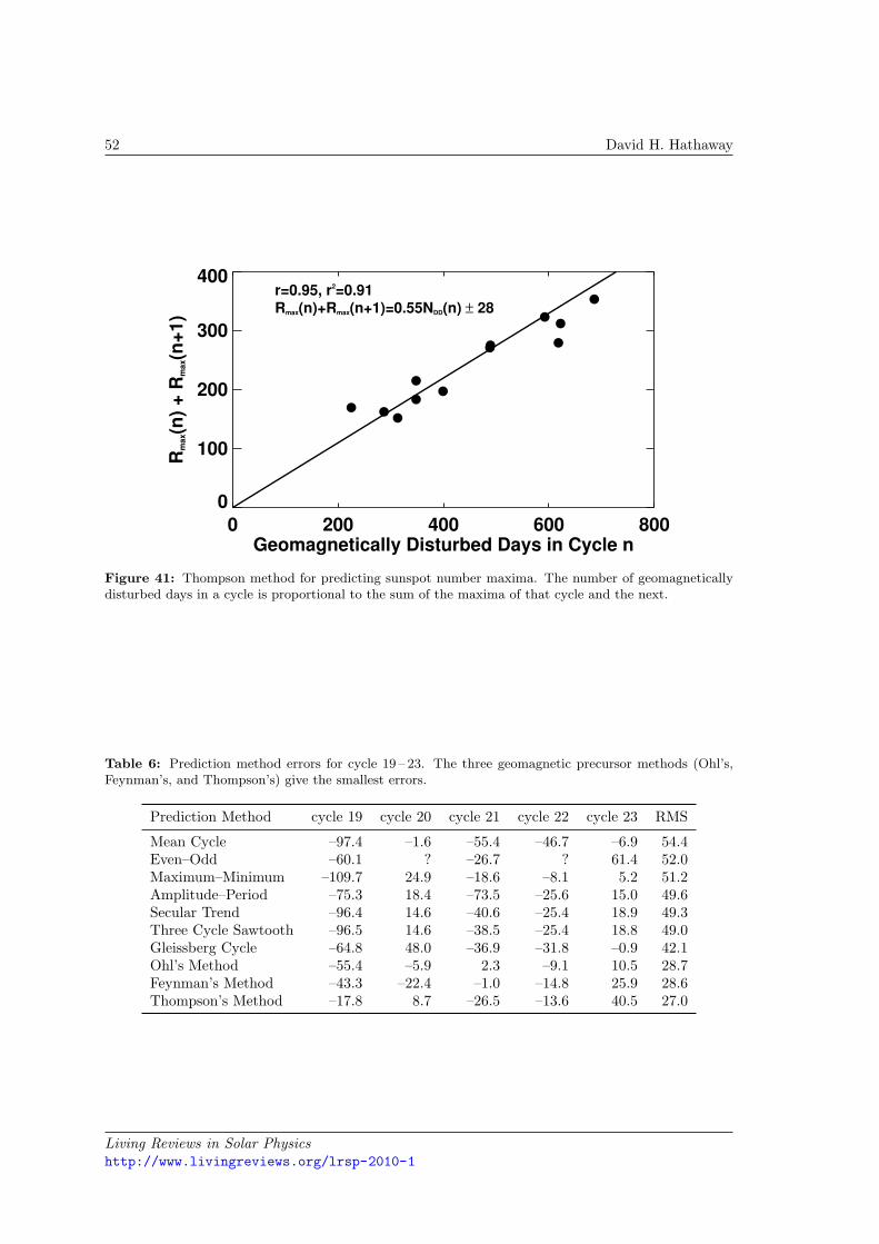
52 David H. Hathaway
0 200 400 600 800Geomagnetically Disturbed Days in Cycle n
0
100
200
300
400
Rm
ax(n
) +
Rm
ax(n
+1
)
r=0.95, r2=0.91Rmax(n)+Rmax(n+1)=0.55NDD(n) ± 28
Figure 41: Thompson method for predicting sunspot number maxima. The number of geomagneticallydisturbed days in a cycle is proportional to the sum of the maxima of that cycle and the next.
Table 6: Prediction method errors for cycle 19 – 23. The three geomagnetic precursor methods (Ohl’s,Feynman’s, and Thompson’s) give the smallest errors.
Prediction Method cycle 19 cycle 20 cycle 21 cycle 22 cycle 23 RMS
Mean Cycle –97.4 –1.6 –55.4 –46.7 –6.9 54.4Even–Odd –60.1 ? –26.7 ? 61.4 52.0Maximum–Minimum –109.7 24.9 –18.6 –8.1 5.2 51.2Amplitude–Period –75.3 18.4 –73.5 –25.6 15.0 49.6Secular Trend –96.4 14.6 –40.6 –25.4 18.9 49.3Three Cycle Sawtooth –96.5 14.6 –38.5 –25.4 18.8 49.0Gleissberg Cycle –64.8 48.0 –36.9 –31.8 –0.9 42.1Ohl’s Method –55.4 –5.9 2.3 –9.1 10.5 28.7Feynman’s Method –43.3 –22.4 –1.0 –14.8 25.9 28.6Thompson’s Method –17.8 8.7 –26.5 –13.6 40.5 27.0
Living Reviews in Solar Physicshttp://www.livingreviews.org/lrsp-2010-1

The Solar Cycle 53
7.4 Predicting future cycle amplitudes based on dynamo theory
Dynamo models for the Sun’s magnetic field and its evolution have led to predictions based onaspects of those models. Schatten et al. (1978) suggested using the strength of the Sun’s polarfield as a predictor for the amplitude of the following cycle based on the Babcock (1961) dynamomodel. In the Babcock model the polar field at minimum is representative of the poloidal field thatis sheared out by differential rotation to produce the toroidal field that erupts as active regionsduring the following cycle. Diffusion of the erupting active region magnetic field and transportby the meridional flow (along with the Joy’s Law tilt of these active regions) then leads to theaccumulation of opposite polarity fields at the poles and the ultimate reversal of the polar fieldsas shown in Figure 15.
Good measurements of the Sun’s polar field are difficult to obtain. The field is weak andpredominantly radially directed and thus nearly transverse to our line-of-sight. This makes theZeeman signature weak and prone to the detrimental effects of scattered light. Nevertheless,systematic measurements of the polar fields have been made at the Wilcox Solar Observatory since1976 and have been used by Schatten and his colleagues to predict cycles 21 – 24. These polarfield measurements are shown in Figure 42 along with smoothed sunspot numbers. While thephysical basis for these predictions is appealing, the fact that the necessary measurements are onlyavailable for the last three cycles is a distinct problem. It is unclear when the measurements shouldbe taken. Predictions by this group for previous cycles have given different values at different times.The RMS differences between the published predictions and the observed cycle amplitudes suggestthat these predictions are about as good as the geomagnetic precursor predictions. The polarfields are obviously much weaker during the current minimum. This has led to a prediction of𝑅max(24) = 75 ± 8 by Svalgaard et al. (2005) – about half the size of the previous three cyclesbased on the polar fields being about half as strong. While in previous minima the strength of thepolar fields (as represented by the average of the absolute field strength in the north and in thesouth) varied as minimum approached, this did not happen on the approach to cycle 24 minimumin late 2008. This suggests that the prediction made in 2005 still holds.
Wilcox Solar Observatory Polar Fields
1970 1980 1990 2000 2010Date
-300
-200
-100
0
100
200
Po
lar
Fie
ld S
tren
gth
(µ
T)
21 22 23
North South Sunspot Number - 300
Figure 42: Polar magnetic fields as measured at the Wilcox Solar Observatory. The average of the northand south field strengths near the time of sunspot cycle minimum is expected to be an indicator for theamplitude of the next sunspot cycle.
Over the last decade dynamo models have started to include the effect of the Sun’s meridional
Living Reviews in Solar Physicshttp://www.livingreviews.org/lrsp-2010-1

54 David H. Hathaway
circulation and found that it can play a significant role in the magnetic dynamo (cf. Dikpati andCharbonneau, 1999). In these models the speed of the meridional circulation sets the cycle periodand influences both the strength of the polar fields and the amplitudes of following cycles. Twopredictions have recently been made based on flux transport dynamos with assimilated data – withvery different results.
Dikpati et al. (2006) predicted an amplitude for cycle 24 of 150 – 180 using a flux transportdynamo that included a rotation profile and a near surface meridional flow based on helioseismicobservations. They modeled the axisymmetric poloidal and toroidal magnetic field using a merid-ional flow that returns to the equator at the base of the convection zone and used two source termsfor the poloidal field – one at the surface due to the Joy’s Law tilt of the emerging active regionsand one in the tachocline due to hydrodynamic and MHD instabilities. The diffusivity in the modelis a function of depth with a surface diffusivity of 5 × 1012 cm2 s–1 falling to 5 × 1010 cm2 s–1 at𝑟 = 0.9 𝑅⊙. They drive the model with a surface source of poloidal field that depends upon thesunspot areas observed since 1874. Measurements of the meridional flow speed prior to 1996 arehighly uncertain (cf. Hathaway, 1996) so they maintained a constant flow speed prior to 1996 andforced each of those earlier cycles to have a constant period as a consequence. The surface poloidalsource term drifted linearly from 30° to 5° over each cycle with an amplitude that depended on theobserved sunspot areas. They based their prediction on the strength of the toroidal field producedin the tachocline. They found excellent agreement between this toroidal field strength and theamplitude of each of the last eight cycles (the four earlier cycles – during the initialization phase– were also well fit but not with the degree of agreement of the later cycles). The correlation theyfind between the predicted toroidal field and the cycle amplitudes is similar to that found with thegeomagnetic precursors and polar field strength indicators. When they kept the meridional flowspeed at the same constant level during cycle 23 they found 𝑅max(24) ∼ 180. When they allowedthe meridional flow speed to drop by 40% as was seen from 1996 – 2002 they found 𝑅max(24) ∼ 150and further predicted that cycle 24 would start late.
Choudhuri et al. (2007) predicted an amplitude for cycle 24 of 80 using a similar flux-transportdynamo but with the surface poloidal field at minimum as the assimilated data. They used asimilar axisymmetric model for the poloidal and toroidal fields but with a meridional flow thatextends below the base of the convection zone and a diffusivity that remains high throughout theconvection zone. In their model the toroidal field in the tachocline produces flux eruptions whenits strength exceeds a given limit. They compare the number of eruptions to the observed sunspotnumbers and use this as the predictor for cycle 24. They assimilate data by instantaneouslychanging the poloidal field at minimum throughout most of the convection zone to make it matchthe dipole moment obtained from the Wilcox Solar Observatory observations (Figure 41). Theyfound an excellent fit to the last three cycles (the full extent of the data) and found 𝑅max(24) ∼ 80,in agreement with the polar field prediction of Svalgaard et al. (2005).
Criticism has been leveled against all of these dynamo-based predictions. Dikpati et al. (2006)criticized the use of polar field strengths to predict the sunspot cycle peak that follows by four yearsby questioning how those fields could be carried down to the low latitude tachocline in such a shorttime. Cameron and Schussler (2007) produced a simplified 1D flux transport model and showedthat with similar parameters to those used by Dikpati et al. (2006) the flux transport across theequator was an excellent predictor for the amplitude of the next cycle but the predictive skill waslost when more realistic parameterizations of the active region emergence were used. Yeates et al.(2008) compared an advection-dominated model like that of Dikpati et al. (2006) to a diffusion-dominated models like that of Choudhuri et al. (2007) and concluded that the diffusion-dominatedmodel was better because it gave a better fit to the relationship between meridional flow speedand cycle amplitude. Dikpati et al. (2008a) returned with a study of the use of polar fields andcross equatorial flux as predictors of cycle amplitudes and concluded that their tachocline toroidalflux was the best indicator. Furthermore, they found that the polar fields followed the current
Living Reviews in Solar Physicshttp://www.livingreviews.org/lrsp-2010-1

The Solar Cycle 55
cycle so that the weak polar fields at this minimum are due to the weakened meridional flow. Thestrongest criticism of these dynamo-based predictions was give by Tobias et al. (2006) and Bushbyand Tobias (2007). They conclude that the solar dynamo is deterministically chaotic and thusinherently unpredictable.
Living Reviews in Solar Physicshttp://www.livingreviews.org/lrsp-2010-1

56 David H. Hathaway
8 Conclusions
Understanding the solar cycle remains as one of the biggest problems in solar physics. It is alsoone of the oldest. Several key features of the solar cycle have been reviewed here and must beexplained by any viable theory or model.
• The solar cycle has a period of about 11 years but varies in length with a standard deviationof about 14 months.
• Each cycle appears as an outburst of activity that overlaps with both the preceding andfollowing cycles by about 18 months.
• Solar cycles are asymmetric with respect to their maxima – the rise to maximum is shorterthan the decline to minimum and the rise time is shorter for larger amplitude cycles.
• Big cycles usually start early and leave behind a short preceding cycle and a high minimumof activity.
• Sunspots erupt in low latitude bands on either side of the equator and these bands drifttoward the equator as each cycle progresses.
• The activity bands widen during the rise to maximum and narrow during the decline tominimum.
• At any time one hemisphere may dominate over the other but the northern and southernhemispheres never get completely out of phase.
• Sunspots erupt in groups extended in longitude but more constrained in latitude with onemagnetic polarity associated with the leading (in the direction of rotation) spots and theopposite polarity associated with the following spots.
• The magnetic polarities of active regions reverse from northern to southern hemispheres andfrom one cycle to the next.
• The polar fields reverse polarity during each cycle at about the time of cycle maximum.
• The leading spots in a group are positioned slightly equatorward of the following spots andthis tilt increases with latitude.
• Cycle amplitudes exhibit weak quasi-periodicities like the 7 to 8-cycle Gleissberg Cycle.
• Cycle amplitudes exhibit extended periods of inactivity like the Maunder Minimum.
• Solar activity exhibits quasi-periodicities at time scales shorter than 11 years.
• Predicting the level of solar activity for the remainder of a cycle is reliable 2 – 3 years aftercycle minimum.
• Predictions for the amplitude of a cycle based on the Sun’s polar field strength or on geo-magnetic activity near cycle minimum are significantly better than using the climatologicalmean.
Living Reviews in Solar Physicshttp://www.livingreviews.org/lrsp-2010-1
The Solar Cycle 57
References
Abbot, C.G., Fowle, F.E. and Aldrich, L.B., 1913, “The Variation of the Sun”, Astrophys. J., 38,181–186. [DOI], [ADS] (Cited on page 14.)
Ahluwalia, H.S., 1998, “The predicted size of cycle 23 based on the inferred three-cycle quasi-periodicity of the planetary index 𝐴𝑝”, J. Geophys. Res., 103(A6), 12,103–12,109. [DOI], [ADS]
(Cited on page 48.)
Babcock, H.D., 1959, “The Sun’s Polar Magnetic Field”, Astrophys. J., 130, 364–365. [DOI], [ADS]
(Cited on page 17.)
Babcock, H.W., 1961, “The topology of the Sun’s magnetic field and the 22-year cycle”, Astrophys.J., 133, 572–587. [DOI], [ADS] (Cited on page 53.)
Bachmann, K.T. and White, O.R., 1994, “Observations of Hysteresis in Solar Cycle VariationsAmong Seven Solar Activity Indicators”, Solar Phys., 150, 347–357. [DOI], [ADS] (Cited onpages 14 and 34.)
Bai, T., 2003, “Hot Spots for Solar Flares Persisting for Decades: Longitude Distributions of Flaresof Cycles 19-23”, Astrophys. J., 585, 1114–1123. [DOI], [ADS] (Cited on page 40.)
Bai, T. and Cliver, E.W., 1990, “A 154 Day Periodicity in the Occurrence Rate of Proton Flares”,Astrophys. J., 363, 299–309. [DOI], [ADS] (Cited on page 45.)
Ballester, J.L., Oliver, R. and Carbonell, M., 2002, “The Near 160 Day Periodicity in the Photo-spheric Magnetic Flux”, Astrophys. J., 566, 505–511. [DOI], [ADS] (Cited on page 45.)
Balmaceda, L.A., Solanki, S.K., Krivova, N.A. and Foster, S., 2009, “A homogeneous databaseof sunspot areas covering more than 130 years”, J. Geophys. Res., 114, A07104. [DOI], [ADS],[arXiv:0906.0942] (Cited on page 11.)
Baranyi, T., Gyori, L., Ludmany, A. and Coffey, H.E., 2001, “Comparison of sunspot area databases”, Mon. Not. R. Astron. Soc., 323, 223–230. [DOI], [ADS] (Cited on page 11.)
Bazilevskaya, G.A., Krainev, M.B., Makhmutov, V.S., Fluckiger, E.O. and Sladkova, A.I. Storini,M., 2000, “Structure and Maximum Phase of Solar Cycles 21 and 22”, Solar Phys., 197, 157–174.[DOI], [ADS] (Cited on page 46.)
Becker, U., 1954, “Die Eigenbewegung der Sonnenflecken in Breite”, Z. Astrophys., 34, 129–136.[ADS] (Cited on page 37.)
Beer, J., Blinov, A., Bonani, G., Finkel, R.C., Hofmann, H.J., Lehmann, B., Oeschger, H., Sigg,A., Schwander, J., Staffelbach, T., Stauffer, B., Suter, M. and Wotfli, W., 1990, “Use of 10Be inpolar ice to trace the 11-year cycle of solar activity”, Nature, 347, 164–166. [DOI], [ADS] (Citedon page 24.)
Beer, J., Tobias, S. and Weiss, N., 1998, “An active Sun throughout the Maunder Minimum”,Solar Phys., 181, 237–249. [DOI], [ADS] (Cited on page 42.)
Benevolenskaya, E.E., 1995, “Double Magnetic Cycle of Solar Activity”, Solar Phys., 161, 1–8.[DOI], [ADS] (Cited on page 46.)
Benz, A.O., 2008, “Flare Observations”, Living Rev. Solar Phys., 5, lrsp-2008-1. URL (cited on 3February 2010):http://www.livingreviews.org/lrsp-2008-1 (Cited on page 18.)
Living Reviews in Solar Physicshttp://www.livingreviews.org/lrsp-2010-1

58 David H. Hathaway
Berdyugina, S.V. and Usoskin, I.G., 2003, “Active longitudes in sunspot activity: Century scalePersistence”, Astron. Astrophys., 405, 1121–1128. [DOI], [ADS] (Cited on page 40.)
Berggren, A.-M., Beer, J., Possnertt, G., Aldahan, A., Kubik, P., Christl, M., Johnsen, S.J.,Abreu, J. and Vinther, B.M., 2009, “A 600-year annual 10Be record from the NGRIP ice core,Greenland”, Geophys. Res. Lett., 36, L11801. [DOI], [ADS] (Cited on page 44.)
Bogart, R.S., 1982, “Recurrence of Solar Activity: Evidence for Active Longitudes”, Solar Phys.,76, 155–165. [DOI], [ADS] (Cited on page 40.)
Bray, R.J. and Loughhead, R.E., 1965, Sunspots, Wiley, New York (Cited on page 6.)
Brown, G.M., 1976, “What determines sunspot maximum?”, Mon. Not. R. Astron. Soc., 174,185–189. [ADS] (Cited on page 48.)
Bumba, V. and Henja, L., 1991, “Low-latitude Active Longitudes on the Sun and in InterplanetarySpace”, Bull. Astron. Inst. Czech., 42, 76–84. [ADS] (Cited on page 40.)
Bumba, V. and Howard, R., 1965, “Large-scale Distribution of Solar Magnetic Fields”, Astrophys.J., 141, 1502–1512. [DOI], [ADS] (Cited on page 40.)
Bushby, P.J. and Tobias, S.T., 2007, “On predicting the solar cycle using mean-field models”,Astrophys. J., 661, 1289–1296. [DOI], [ADS] (Cited on page 55.)
Cameron, R. and Schussler, M., 2007, “Solar cycle prediction using precursors and flux transportmodels”, Astrophys. J., 659, 801–811. [DOI], [ADS] (Cited on pages 50 and 54.)
Carbonell, M., Oliver, R. and Ballester, J.L., 1993, “On the asymmetry of solar activity”, Astron.Astrophys., 274, 497–504. [ADS] (Cited on page 38.)
Carrington, R.C., 1858, “On the Distribution of the Solar Spots in Latitude Since the Beginningof the Year 1854; with a map”, Mon. Not. R. Astron. Soc., 19, 1–3. [ADS] (Cited on page 36.)
Carrington, R.C., 1859, “Description of a Singular Appearance seen in the Sun on September 1,1859”, Mon. Not. R. Astron. Soc., 20, 13–15. [ADS] (Cited on page 18.)
Charbonneau, P., 2005, “Dynamo Models of the Solar Cycle”, Living Rev. Solar Phys., 2, lrsp-2005-2. URL (cited on 3 February 2010):http://www.livingreviews.org/lrsp-2005-2 (Cited on page 5.)
Choudhuri, A.R., Chatterjee, P. and Jiang, J., 2007, “Predicting solar cycle 24 with a solar dynamomodel”, Phys. Rev. Lett., 98, 131103. [DOI], [ADS] (Cited on page 54.)
Clark, D.H. and Stephenson, F.R., 1978, “An Interpretation of Pre-Telescopic Records from theOrient”, Quart. J. R. Astron. Soc., 19, 387–410. [ADS] (Cited on page 6.)
Dikpati, M. and Charbonneau, P., 1999, “A Babcock-Leighton flux transport dynamo with solar-like differential rotation”, Astrophys. J., 518, 508–520. [DOI], [ADS] (Cited on page 54.)
Dikpati, M., de Toma, G. and Gilman, P.A., 2006, “Predicting the strength of solar cycle 24 usinga flux-transport dynamo-based tool”, Geophys. Res. Lett., 33, L05102. [DOI], [ADS] (Cited onpage 54.)
Dikpati, M., de Toma, G. and Gilman, P.A., 2008a, “Polar flux, cross-equatorial flux, and dynamogenerated tachocline toroidal flux as predictors of solar cycles”, Astrophys. J., 675, 920–930.[DOI], [ADS] (Cited on page 54.)
Living Reviews in Solar Physicshttp://www.livingreviews.org/lrsp-2010-1

The Solar Cycle 59
Dikpati, M., Gilman, P.A. and de Toma, G., 2008b, “The Waldmeier Effect: An Artifact of theDefinition of Wolf Sunspot Number?”, Astrophys. J. Lett., 673, L99–L101. [DOI], [ADS] (Citedon page 34.)
“Latest Solar Radio Flux Report”, project homepage, Space Weather Canada. URL (cited on 3February 2010):hhttp://www.spaceweather.ca/sx-4-eng.php (Cited on page 14.)
Eddy, J.A., 1976, “The Maunder Minimum”, Science, 192, 1189–1202. [DOI], [ADS] (Cited onpage 42.)
Eddy, J.A., 1977, “Historical evidence for the existence of the solar cycle”, in The Solar Output andIts Variation, (Ed.) White, O.R., Proceedings of a Workshop, held in Boulder, Colorado, April26 – 28, 1976, pp. 55–71, Colorado Associated University Press, Boulder, CO. [ADS] (Cited onpage 31.)
Elling, W. and Schwentek, H., 1992, “Fitting the Sunspot Cycles 10–21 by a Modified 𝐹 -Distribution Density Function”, Solar Phys., 137, 155–165. [DOI], [ADS] (Cited on pages 33and 47.)
Ferreira, S.E. and Potgieter, M.S., 2004, “Long-Term Cosmic Ray Modulation in the Heliosphere”,Astrophys. J., 603, 744–752. [ADS] (Cited on page 23.)
Feynman, J., 1982, “Geomagnetic and Solar Wind Cycles, 1900-1975”, J. Geophys. Res., 87(A8),6153–6166. [DOI], [ADS] (Cited on pages 21 and 50.)
Fligge, M. and Solanki, S.K., 1997, “Inter-cycle Variations of Solar Irradiance: Sunspot Areas asa Pointer”, Solar Phys., 173, 427–439. [DOI], [ADS] (Cited on page 11.)
Forbush, S.E., 1954, “World-Wide Cosmic-Ray Variations, 1937–1952”, J. Geophys. Res., 59, 525–542. [ADS] (Cited on page 23.)
Frohlich, C. and Lean, J., 1998, “The Sun’s Total Irradiance: Cycles, Trends and Related ClimateChange Uncertainties since 1976”, Geophys. Res. Lett., 25, 4377–4380. [DOI], [ADS] (Cited onpage 15.)
Garcia, A. and Mouradian, Z., 1998, “The Gleissberg Cycle of Minima”, Solar Phys., 180, 495–498.[DOI], [ADS] (Cited on page 43.)
Gleissberg, M.N., 1939, “A long-periodic Fluctuation of the Sun-spot Numbers”, Observatory , 62,158–159. [ADS] (Cited on pages 43 and 48.)
Gnevyshev, M.N., 1963, “The corona and the 11-year cycle of solar activity”, Sov. Astron., 7,311–318. [ADS] (Cited on page 46.)
Gnevyshev, M.N., 1967, “On the 11-Years Cycle of Solar Activity”, Solar Phys., 1, 107–120. [DOI],[ADS] (Cited on page 46.)
Gnevyshev, M.N., 1977, “Essential features of the 11-year solar cycle”, Solar Phys., 51, 175–183.[DOI], [ADS] (Cited on page 46.)
Gnevyshev, M.N. and Ohl, A.I., 1948, “On the 22-year cycle of solar activity”, Astron. Zh., 25,18–20 (Cited on pages 43 and 48.)
Haigh, J.D., 2007, “The Sun and the Earth’s Climate”, Living Rev. Solar Phys., 4, lrsp-2007-2.URL (cited on 3 February 2010):http://www.livingreviews.org/lrsp-2007-2 (Cited on page 5.)
Living Reviews in Solar Physicshttp://www.livingreviews.org/lrsp-2010-1

60 David H. Hathaway
Hale, G.E., 1908, “On the Probable Existence of a Magnetic Field in Sun-Spots”, Astrophys. J.,28, 315–343. [DOI], [ADS] (Cited on page 17.)
Hale, G.E., Ellerman, F., Nicholson, S.B. and Joy, A.H., 1919, “The Magnetic Polarity of Sun-Spots”, Astrophys. J., 49, 153–178. [DOI], [ADS] (Cited on pages 17 and 18.)
Harvey, K.L. and White, O.R., 1999, “What is solar cycle minimum?”, J. Geophys. Res., 104(A9),19,759–19,764. [DOI], [ADS] (Cited on page 27.)
Hathaway, D.H., 1996, “Doppler measurements of the Sun’s meridional flow”, Astrophys. J., 460,1027–1033. [DOI], [ADS] (Cited on page 54.)
Hathaway, D.H. and Wilson, R.M., 2006, “Geomagnetic activity indicates large amplitude forsunspot cycle 24”, Geophys. Res. Lett., 33, L18101. [DOI], [ADS] (Cited on page 50.)
Hathaway, D.H., Wilson, R.M. and Reichmann, E.J., 1994, “The Shape of the Sunspot Cycle”,Solar Phys., 151, 177–190. [DOI], [ADS] (Cited on pages 33, 34, 35, 36, and 47.)
Hathaway, D.H., Wilson, R.M. and Reichmann, E.J., 1999, “A synthesis of solar cycle predictiontechniques”, J. Geophys. Res., 104(A10), 22,375–22,388. [DOI], [ADS] (Cited on pages 29, 43,and 50.)
Hathaway, D.H., Wilson, R.M. and Reichmann, E.J., 2002, “Group Sunspot Numbers: SunspotCycle Characteristics”, Solar Phys., 211, 357–370. [ADS] (Cited on pages 10, 11, 31, 34, and 42.)
Hathaway, D.H., Nandy, D., Wilson, R.M. and Reichmann, E.J., 2003, “Evidence that a DeepMeridional Flow Sets the Sunspot Cycle Period”, Astrophys. J., 589, 665–670. [DOI], [ADS]
(Cited on page 36.)
Henney, C.J. and Harvey, J.W., 2002, “Phase Coherence of Solar Magnetic Activity”, Solar Phys.,207, 199–218. [DOI], [ADS] (Cited on page 40.)
Hodgson, R., 1859, “On a Curious Appearance seen in the Sun”, Mon. Not. R. Astron. Soc., 20,15–16. [ADS] (Cited on page 18.)
Holland, R.L. and Vaughn, W.W., 1984, “Lagrangian Least-Squares Prediction of Solar Flux(𝐹10.7)”, J. Geophys. Res., 89, 11–16. [DOI], [ADS] (Cited on page 14.)
Howe, R. Christensen-Dalsgaard, J., Hill, F., Komm, R., Schou, J., Thompson, M.J. and Toomre,J., 2007, “Temporal variations in the solar rotation at the bottom of the convection zone: Thecurrent status”, Adv. Space Res., 40, 915–918. [ADS] (Cited on page 46.)
Howe, R., Christensen-Dalsgaard, J., Hill, F., Komm, R.W., Larsen, R.M., Schou, J., Thompson,M.J. and Toomre, J., 2000, “Dynamic Variations at the Base of the Solar Convection Zone”,Science, 287, 2456–2460. [DOI], [ADS] (Cited on page 46.)
Hoyt, D.V. and Schatten, K.H., 1998, “Group Sunspot Numbers: A New Solar Activity Recon-struction”, Solar Phys., 179, 189–219. [ADS] (Cited on pages 10 and 42.)
Javaraiah, J., 2007, “North–south asymmetry in solar activity: predicting the amplitude of thenext solar cycle”, Mon. Not. R. Astron. Soc., 377, L34–L38. [DOI], [ADS], [astro-ph/0701923]
(Cited on page 48.)
Living Reviews in Solar Physicshttp://www.livingreviews.org/lrsp-2010-1

The Solar Cycle 61
Keller, C.U. (NSO Staff), 1998, “SOLIS – A modern Facility for Synoptic Solar Observations”, inCool Stars, Stellar Systems and the Sun: Tenth Cambridge Workshop, (Eds.) Donahue, R.A.,Bookbinder, J.A., Proceedings of a meeting held at Cambridge, Massachusetts, 15 – 19 July1997, vol. 154 of ASP Conference Series, pp. 636–649, Astronomical Society of the Pacific, SanFrancisco. [ADS] (Cited on page 17.)
Lean, J., 1990, “Evolution of the 155 Day Periodicity in Sunspot Areas During Solar Cycles 12 to21”, Astrophys. J., 363, 718–727. [DOI], [ADS] (Cited on page 45.)
Legrand, J.-P. and Simon, P.A., 1985, “Some solar cycle phenomena related to the geomagneticactivity from 1868 to 1980. I. The shock events, or the interplanetary expansion of the toroidalfield”, Astron. Astrophys., 152, 199–204. [ADS] (Cited on page 21.)
Lockwood, M., Stamper, R. and Wild, M.N., 1999, “A doubling of the Sun’s coronal magnetic fieldduring the past 100 years”, Nature, 399, 437–439. [DOI], [ADS] (Cited on page 21.)
MacQueen, R.M., Eddy, J.A., Gosling, J.T., Hildner, E., Munro, R.H., Newkirk Jr, G.A., Poland,A.I. and Ross, C.L., 1974, “The Outer Solar Corona as Observed from Skylab: PreliminaryResults”, Astrophys. J. Lett., 187, L85–L88. [DOI], [ADS] (Cited on page 19.)
Masarik, J. and Beer, J., 1999, “Simulation of particle fluxes and cosmogenic nuclide productionin the Earth’s atmosphere”, J. Geophys. Res., 104(D10), 12,099–12,111. [DOI], [ADS] (Citedon page 24.)
Maunder, E.W., 1890, “Professor Spoerer’s Researches on Sun-spots”, Mon. Not. R. Astron. Soc.,50, 251–252. [ADS] (Cited on pages 37 and 42.)
Maunder, E.W., 1903, “Spoerer’s Law of Zones”, Observatory , 26, 329–330. [ADS] (Cited onpage 13.)
Maunder, E.W., 1904, “Note on the Distribution of Sun-spots in Heliographic Latitude, 1874 to1902”, Mon. Not. R. Astron. Soc., 64, 747–761. [ADS] (Cited on pages 13 and 37.)
Mayaud, P.N., 1972, “The 𝑎𝑎 indices: a 100-year series characterizing the magnetic activity”, J.Geophys. Res., 77, 6870–6874. [DOI], [ADS] (Cited on page 19.)
McKinnon, J.A., 1987, Sunspot Numbers: 1610-1985 (based on The Sunspot-Activity in the Years1610-1960, by Prof. M. Waldmeier, Copyright 1961, Swiss Federal Observatory, Zurich, Switzer-land), UAG Reports UAG-95, National Geophysical Data Center, NOAA, Boulder, CO (Citedon page 25.)
McNish, A.G. and Lincoln, J.V., 1949, “Prediction of sunspot numbers”, Eos Trans. AGU , 30,673–685 (Cited on page 47.)
Miklailutsa, V.P. and Makarova, V.V., 1994, “The Sector Structure of the Active Longitudes inSolar Cycles”, Solar Phys., 155, 391–400. [ADS] (Cited on page 40.)
Mursula, K., Zieger, B. and Vilppola, J.H., 2003, “Mid-term Quasi-periodicities in GeomagneticActivity During the Last 15 Solar Cycles: Connection to Solar Dynamo Strength”, Solar Phys.,212, 201–207. [DOI], [ADS] (Cited on page 46.)
Newton, H.W. and Milsom, A.S., 1955, “Note on the observed differences in spottedness of theSun’s northern and southern hemispheres”, Mon. Not. R. Astron. Soc., 115, 398–404. [ADS]
(Cited on page 38.)
Living Reviews in Solar Physicshttp://www.livingreviews.org/lrsp-2010-1

62 David H. Hathaway
“Sunspot Number Data via FTP”, project homepage, NOAA National Geophysical Data Center(NGDC). URL (cited on 3 February 2010):http://www.ngdc.noaa.gov/stp/SOLAR/ftpsunspotnumber.html (Cited on page 10.)
Nordemann, D.J.R., 1992, “Sunspot Number Time Series: Exponential Fitting and Solar Behav-ior”, Solar Phys., 141, 199–202. [ADS] (Cited on page 33.)
Noyes, R.W., 1982, The Sun, Our Star , The Harvard Books on Astronomy, Harvard UniversityPress, Cambridge, MA (Cited on page 6.)
Ogurtsov, M.G., Nagovitsyn, Y.A., Kocharov, G.E. and Jungner, H., 2002, “Long-period cycles ofthe Sun’s activity recorded in direct solar data and proxies”, Solar Phys., 211, 371–394. [DOI],[ADS] (Cited on page 43.)
Ohl, A.I., 1966, “Forecast of sunspot maximum number of cycle 20”, Soln. Dannye, (12), 84 (Citedon page 48.)
Parker, E.N., 1965, “The passage of energetic charged particles through interplanetary space”,Planet. Space Sci., 13, 9–49. [DOI], [ADS] (Cited on page 23.)
Pulkkinen, T., 2007, “Space Weather: Terrestrial Perspectives”, Living Rev. Solar Phys., 4, lrsp-2007-1. URL (cited on 3 February 2010):http://www.livingreviews.org/lrsp-2007-1 (Cited on page 5.)
“Royal Greenwich Observatory – USAF/NOAA Sunspot Data”, project homepage, NASA / Mar-shall Space Flight Center. URL (cited on 3 February 2010):http://solarscience.msfc.nasa.gov/greenwch.shtml (Cited on page 13.)
Ribes, J.C. and Nesme-Ribes, E., 1993, “The solar sunspot cycle in the Maunder minimum AD1645to AD 1715”, Astron. Astrophys., 276, 549–563. [ADS] (Cited on page 42.)
Rieger, E., Share, G.H., Forrest, D.J., Kanbach, G., Reppin, C. and Chupp, E.L., 1984, “A 154-dayperiodicity in the occurrence of hard solar flares?”, Nature, 312, 623–625. [DOI], [ADS] (Citedon page 45.)
Roy, J.-R., 1977, “The North–South Distribution of Major Solar Flare Events, Sunspot MagneticClasses and Sunspot Areas (1955–1974)”, Solar Phys., 52, 53–61. [DOI], [ADS] (Cited onpage 37.)
Rozelot, J.P., 1994, “On the stability of the 11-year solar cycle period (and a few others)”, SolarPhys., 149, 149–154. [DOI], [ADS] (Cited on page 43.)
Sawyer, C., 1968, “Statistics of Solar Active Regions”, Annu. Rev. Astron. Astrophys., 6, 115–134.[DOI], [ADS] (Cited on page 40.)
Schatten, K.H. and Sofia, S., 1987, “Forecast of an exceptionally large even-numbered solar cycle”,Geophys. Res. Lett., 14, 632–635. [DOI], [ADS] (Cited on page 50.)
Schatten, K.H., Scherrer, P., Svalgaard, L. and Wilcox, J.M., 1978, “Using dynamo theory topredict the sunspot number during solar cycle 21”, Geophys. Res. Lett., 5, 411–414. [DOI], [ADS]
(Cited on page 53.)
Scherrer, P.H., Bogart, R.S., Bush, R.I., Hoeksema, J.T., Kosovichev, A.G., Schou, J., Rosenberg,W., Springer, L., Tarbell, T.D., Title, A., Wolfson, C.J. and Zayer, I. (MDI Engineering Team),1995, “The Solar Oscillations Investigation – Michelson Doppler Imager”, Solar Phys., 162,129–188. [DOI], [ADS] (Cited on page 18.)
Living Reviews in Solar Physicshttp://www.livingreviews.org/lrsp-2010-1

The Solar Cycle 63
Schwabe, H., 1844, “Sonnen-Beobachtungen im Jahre 1843”, Astron. Nachr., 21(495), 233–236.[DOI], [ADS] (Cited on page 6.)
Sheeley Jr, N.R., 1991, “Polar Faculae: 1906–1990”, Astrophys. J., 374, 386–389. [ADS] (Citedon page 17.)
Sheeley Jr, N.R., 2005, “Surface Evolution of the Sun’s Magnetic Field: A Historical Review of theFlux-Transport Mechanism”, Living Rev. Solar Phys., 2, lrsp-2005-5. URL (cited on 3 February2010):http://www.livingreviews.org/lrsp-2005-5 (Cited on page 43.)
“Solar Influences Data Analysis Center - SIDC”, institutional homepage, Royal Observatory ofBelgium. URL (cited on 3 February 2010):http://sidc.oma.be/ (Cited on page 10.)
Solanki, S.K., Krivova, N.A., Schussler, M. and Fligge, M., 2002, “Search for a relationship betweensolar cycle amplitude and length”, Astron. Astrophys., 396, 1029–1035. [DOI], [ADS] (Cited onpage 36.)
Solanki, S.K., Usoskin, I.G., Kromer, B., Schussler, M. and Beer, J., 2004, “Unusual activity ofthe Sun during the previous 11,000 years”, Nature, 431, 1084–1087. [DOI], [ADS] (Cited onpage 43.)
Spoerer, M.G., 1889, “Sur les differences que presentent l’hemisphere nord et l’hemisphere sud dusoleil”, Bull. Astron. (Paris), 6, 60–63. [ADS] (Cited on page 37.)
Stewart, J.Q. and Panofsky, H.A.A., 1938, “The Mathematical Characteristics of Sunspot Varia-tions”, Astrophys. J., 88, 385–407. [DOI], [ADS] (Cited on pages 33 and 47.)
Stuiver, M. and Quay, P.D., 1980, “Changes in Atmospheric Carbon-14 Attributed to a VariableSun”, Science, 207, 11–19. [DOI], [ADS] (Cited on page 24.)
Suess, H.E., 1980, “The radiocarbon record in tree rings of the last 8000 years”, Radiocarbon, 22,200–209 (Cited on page 44.)
Svalgaard, L., Cliver, E.W. and Le Sager, P., 2004, “IHV: a new long-term geomagnetic index”,Adv. Space Res., 34, 436–439. [DOI], [ADS] (Cited on page 19.)
Svalgaard, L., Cliver, E.W. and Kamide, Y., 2005, “Sunspot cycle 24: Smallest cycle in 100 years?”,Geophys. Res. Lett., 32, L01 104. [DOI], [ADS] (Cited on pages 53 and 54.)
Tapping, K.F. and Charrois, D.P., 1994, “Limits to the Accuracy of the 10.7 cm Flux”, SolarPhys., 150, 305–315. [DOI], [ADS] (Cited on page 13.)
Thompson, J.R., 1993, “A technique for predicting the amplitude of the solar cycle”, Solar Phys.,148, 383–388. [DOI], [ADS] (Cited on page 50.)
Tobias, S., Hughes, D. and Weiss, N., 2006, “Unpredictable Sun leaves researchers in the dark”,Nature, 442, 26. [DOI], [ADS] (Cited on page 55.)
Tousey, R., 1973, “The Solar Corona”, in Space Research XIII , (Eds.) Rycroft, M.J., Runcorn,S.K., Proceedings of open meetings of working groups on physical sciences of the 15th plenarymeeting of COSPAR, Madrid, Spain, 10 – 24 May, 1972, p. 713, Akademie-Verlag, Berlin. [ADS]
(Cited on page 19.)
Living Reviews in Solar Physicshttp://www.livingreviews.org/lrsp-2010-1

64 David H. Hathaway
Usoskin, I.G., 2008, “A History of Solar Activity over Millennia”, Living Rev. Solar Phys., 5,lrsp-2008-3. URL (cited on 3 February 2010):http://www.livingreviews.org/lrsp-2008-3 (Cited on page 44.)
Vitinskij, Y.I., 1976, “Forecast of the Height of Solar Cycle 21 Using methods Based on the LatitudeDistribution of Sunspots”, Soln. Dannye, (11), 59–63. [ADS] (Cited on page 36.)
Vonmoos, M., Beer, J. and Muscheler, R., 2006, “Large variations in the Holocene solar activity:Constraints from 10Be in the Greenland Ice Core Project ice core”, J. Geophys. Res., 111,A10105. [DOI], [ADS] (Cited on page 44.)
Waldmeier, M., 1935, “Neue Eigenschaften der Sonnenfleckenkurve”, Astron. Mitt. Zurich, 14(133), 105–130. [ADS] (Cited on pages 25, 33, and 34.)
Waldmeier, M., 1939, “Die Zonenwanderung der Sonnenflecken”, Astron. Mitt. Zurich, 14(138),470–481. [ADS] (Cited on page 34.)
Waldmeier, M., 1955, Ergebnisse und Probleme der Sonnenforschung , Geest & Portig, Leipzig, 2ndedn. [ADS] (Cited on page 37.)
Waldmeier, M., 1957, “Der lange Sonnenzyklus”, Z. Astrophys., 43, 149–160. [ADS] (Cited onpage 38.)
Waldmeier, M., 1961, The Sunspot-Activity in the Years 1610-1960 , Schulthess u. Co. / SwissFederal Observatory, Zurich. [ADS] (Cited on page 25.)
Waldmeier, M., 1971, “The Asymmetry of Solar Activity in the Years 1959-1969”, Solar Phys.,20, 332–344. [DOI], [ADS] (Cited on pages 37 and 38.)
Wang, Y.-M. and Sheeley Jr, N.R., 2003, “On the fluctuating component of the Sun’s large-scalemagnetic field”, Astrophys. J., 590, 1111–1120. [DOI], [ADS] (Cited on page 46.)
Wang, Y.-M. and Sheeley Jr, N.R., 2009, “Understanding the geomagnetic precursor of the solarcycle”, Astrophys. J. Lett., 694, L11–L15. [DOI], [ADS] (Cited on page 50.)
Webb, D.F. and Howard, R.A., 1994, “The solar cycle variation of coronal mass ejections and thesolar wind mass flux”, J. Geophys. Res., 99(A3), 4201–4220. [DOI], [ADS] (Cited on page 19.)
Willson, R.C., 1997, “Total Solar Irradiance Trend During Cycles 21 and 22”, Science, 277, 1963–1965. [DOI], [ADS] (Cited on page 15.)
Willson, R.C. and Hudson, H.S., 1988, “Solar luminosity variations in solar cycle 21”, Nature, 332,810–812. [DOI], [ADS] (Cited on page 15.)
Wilson, R.M., 1987, “On the Distribution of Sunspot Cycle Periods”, J. Geophys. Res., 92(A9),10,101–10,104. [DOI], [ADS] (Cited on page 31.)
Wilson, R.M., 1988, “On the Long-term Secular Increase in Sunspot Number”, Solar Phys., 115,397–408. [DOI], [ADS] (Cited on page 42.)
Wilson, R.M., Hathaway, D.H. and Reichmann, E.J., 1998, “An estimate for the size of cycle 23based on near minimum conditions”, J. Geophys. Res., 103(A4), 6595–6603. [DOI], [ADS] (Citedon page 48.)
Wittmann, A.D. and Xu, Z.T., 1987, “A catalogue of sunspot observations from 165 BC to AD1684”, Astron. Astrophys. Suppl., 70, 83–94. [ADS] (Cited on page 6.)
Living Reviews in Solar Physicshttp://www.livingreviews.org/lrsp-2010-1

The Solar Cycle 65
Wolf, R., 1859, “Extract of a Letter from Prof. R. Wolf, of Zurich, to Mr. Carrington, dated Jan.12, 1859”, Mon. Not. R. Astron. Soc., 19, 85–86. [ADS] (Cited on page 25.)
Wolf, R., 1861, “Abstract of his latest Results”, Mon. Not. R. Astron. Soc., 21, 77–78. [ADS]
(Cited on page 7.)
Wolf, R., 1877, Geschichte der Astronomie, vol. 16 of Geschichte der Wissenschaften in Deutsch-land. Neuere Zeit, Oldenbourg, Munchen. Related online version (cited on 9 February 2010):http://ebooks.ethbib.ethz.ch/fulltext/Rara/1681.pdf (Cited on page 6.)
Wolf, R., 1892, “Astronomische Mittheilungen, LXXIX”, Astron. Mitt. Zurich, 79, 317–364. [ADS]
(Cited on page 27.)
Wolfer, A., 1903, “Astronomische Mitteilungen, XCIV”, Astron. Mitt. Zurich, 94, 97–150. [ADS]
(Cited on page 27.)
Yeates, A.R., Nandy, D. and Mackay, D.H., 2008, “Exploring the Physical Basis of Solar Cy-cle Predictions: Flux Transport Dynamics and Persistence of Memory in Advection- versusDiffusion-dominated Solar Convection Zones”, Astrophys. J., 673, 544–556. [DOI], [ADS] (Citedon page 54.)
Living Reviews in Solar Physicshttp://www.livingreviews.org/lrsp-2010-1
Related Documents