The Significance of Beta for Australian Stock Returns€¦ · beta in Australian markets. We discover, however, that betas of portfolios of Australian stocks have a high level of

The Significance of Beta for Australian Stock Returns

by Mike Dempsey

Department of Accounting and Finance, Monash University, Caulfield Campus, Victoria, Melbourne, Australia.

Address for Correspondence: Mike Dempsey Department of Accounting and Finance Faculty of Business and Economics PO Box 197 Monash University VIC 3145 Australia Tel: 61 3 9903 4543 Fax: 61 3 9905 5475 Email: [email protected]

I am indebted to Bernie Bollen for kind assistance in the programming of the data analysis. And I

gratefully acknowledge financial support from the Melbourne Centre for Financial Studies (Cost Centre

B07005 and 1779270). Any errors are my own.

0

The Significance of Beta for Australian Stock Returns

ABSTRACT

Faff (2001) fails to find a statistically significant relation between returns and their

beta in Australian markets. We discover, however, that betas of portfolios of

Australian stocks have a high level of stability, implying that beta is a meaningful

measure of a portfolio’s market risk exposure. Further, by allowing broad

demarcations of firm size and liquidities, we show how beta appears to be rewarded -

not continuously - but discretely across thresholds of firm size and stock liquidity.

We conclude that beta remains relevant in the description of the risk-reward structure

of asset pricing in Australian markets.

1

The Significance of Beta for Australian Stock Returns

1. Introduction

A quote attributed to Eugene Fama: “Beta as the sole variable explaining returns on

stocks is dead” (New York times, February 18, 1992) has been widely disseminated

as: “Beta is dead.” However, the fact that the average returns of stocks might not

accord with their beta as predicted by the CAPM, does not of itself negate the

usefulness of beta as a measure of a stock’s market risk exposure. If a stock’s beta is

stable across time, its beta – by definition - is a meaningful measure of its market

exposure.

Over the period 1931-1991, Fisher Black (1993) (building on the Black,

Jensen Scholes study of 1972) documents strong beta stationarity – leading to the

observation that beta is “even more valuable if the line (of returns against beta) is

flat.” The stability of beta for U.S. stocks is also highlighted in the study by Grundy

and Malkiel (1996) – who in an article entitled “Reports of Beta’s Death have been

Greatly Exaggerated,” observe that portfolios of U.S. stocks formed on high-betas

over the period 1968-1992 consistently fell more in market declines than portfolios of

stocks of low-betas. As the authors point out, their results, ultimately, are a test of the

stability of their beta portfolios.

Notwithstanding, Fama and French (1992, 1993, 1996, and elsewhere) argue

that beta of itself is not an effective variable in explaining the cross-section of stock

returns. Although portfolios comprising higher beta stocks tend to higher returns, the

relationship effectively disappears once firm size is controlled for. In Australian

markets, Durack, Durand and Maller (2004) confirm the findings of Fama and French

2

in finding that the explanatory power of CAPM is poor. Faff (2001) actually fails to

find a statistically significant relation between beta and returns in Australian markets.

Against such findings, the present paper allows for a reappraisal of the

relevance of beta in Australian markets. Our portfolio analysis approach is robust and

allows for an assessment of stock returns across compartmentalized ranges of beta.

We examine also how a stock’s beta is constituted in terms of its “downside” ( )

and “upside” ( ) components (its beta as measured, respectively, over market

downturns and upturns). Additionally, we examine the performances of portfolios

over designated “bull” and “bear” periods of the Australian markets as a function of

their beta. Finally, the paper examines the structure of portfolio returns as a function

of their beta with reference to the average firm size and liquidity of the stocks in the

beta portfolios.

−β

+β

Our findings may be summarized as follows. Our portfolio betas are

sufficiently stable as to be a meaningful measure of a portfolio’s market risk

exposure. Further, this stability is observed over market upturns and downturns,

measured both as monthly variations and as prolonged “bull” and “bear” periods of

the markets. For example, high beta stocks generally decline more than low beta

stocks in bear markets and are thereby fundamentally more risky. Our observations of

the explanatory nature of beta in relation to returns do not however apply

continuously – or even monotonically. Rather, they apply discretely in relation to

broad categories of the stock’s firm size and liquidity.

Within such categories our results may in turn be summarized as follows. We

find that stocks of larger firm size ( > $500 million) dominate the middle range of beta

(0.65 < beta < 1.3), while stocks of small/medium firm size ($150m < firm size <

$500m) dominate both somewhat lower and somewhat higher beta ranges ( 0.25 <

3

beta < 0.65 and 1.3 < beta < 2.0). And portfolio returns increase significantly across

these three ranges of increasing beta. However, within each of these beta/size ranges,

we find that returns are not overly sensitive to their beta. Stocks of the very smallest

firm sizes (firm size < $150m) predominate the extremely low and extremely high

beta ranges (beta < 0.25 and beta > 2.0). We observe that stocks of the lowest beta

have abnormally high returns, which leads to an overall “hockey-stick” return-beta

relationship. These stocks however are characterized by very low trading volumes,

which limit the practical opportunity to arbitrage. The stocks of very high beta with

very high returns are also typically of the lowest firm size. However, these stocks

typically have high liquidity.

We conclude that beta should not be written off either as a meaningful

measure of an asset’s market sensitivity, or as an indicator of the structure of asset

returns in relation to market performances.

The rest of the paper is arranged as follows. In section 2, we outline the data,

measurements of variables, and the methodology. In section 3, we present the results

for the performances of beta portfolios in three sub-sections. In sub-section (i) we

present our results for portfolios formed on beta as well as our observations for the

composition of the portfolio betas in terms of their separate sensitivities to market

upturns and downturns. In sub-section (ii) we present our results for the performance

of the portfolios formed on beta over designated “bull” and “bear” periods. In sub-

section (iii) we present our results for the characteristic composition of the beta

portfolios in terms of the average firm size and liquidity of their stocks. The final

section summarises and concludes the paper.

4

2. Data, variables and methodology

(i) Data

We use data from the AGSM database of ordinary common stocks listed on the

Australian Stock Exchange (ASX) to construct portfolios of stocks. The data set

initially held 450,489 monthly price observations from 3,922 firms trading over 372

months (January 1st, 1974 to December 31st, 2004). From the set, 6,960 monthly

observations were removed due to missing data (not having a valid date or appearing

as duplicate records). In order to calculate a stock’s monthly return, we required that

a security trade in the previous month, and in order to calculate the beta for such

month, we required that a security trade in 35 out of the previous 60 months. This left

a total of 265,535 monthly stock observations for analysis commencing January 1st,

1979. The descriptive statistics of our sample are presented in the central column of

Table 1.

From the SIRCA database, we acquired daily trading volumes. These were

aggregated to give monthly trading volumes for 279,663 observations. Using the

AGSM security code and month this data was matched to the observation from the

AGSM database. This created 190,218 monthly matched observations of monthly

stock returns, stock firm size and stock liquidity. The average market capitalisation of

the reduced sample was $398 million over 2,347 firms (which compares with $349

million over 2,635 firms for the original data set) – which implies that it is the stocks

of smallest market capitalisation that have been removed. Notwithstanding, the range

of firm sizes remained between $27,000 and $46 billion.

(ii) Measurement of variables

On a monthly basis, the variables for the analyses were measured as follows.

5

(a) Measurement of stock returns (ri,t )

Returns (ri,t) are measured as the difference between the closing price at the end of

month t and the closing price at the end of month t-1: ri,t = (pi,t - pi,t-1)/pi,t, where pi,t is

the price of the stock at the end of month t. By associating a portfolio’s return with

the month after the portfolios is formed we seek to eliminate the bias that results from

correlations in measurements, such as high volatility and higher returns. Returns are

excess returns with the risk-free rate proxied as the three-month Treasury bill rate.

(b) Measurement of stock betas ( β i,t)

Beta (β i,t) for each security i at the end of each month t is calculated from the

previous 60 months of historical data as:

ti ,β = )var(

),cov(

M

Mi

rrr

where and are, respectively, the returns from security i the and the market index

M over months m = t-59 to month t. If a security did not trade for at least 35 out of

the previous 60 months it was not included in that month’s (t) calculation.

ir Mr

The upside beta ( ) and downside beta ( ) for each asset i at the end of

each month t is calculated over separate subsets of the previous 60 months of data as:

+β −β

= ti,−β

)|var()|,cov(

MMM

MMMi

rrrrr

μμ

≤≤

= ti ,+β

)|var()|,cov(

MMM

MMMi

rrrrr

μμ

≥≥

where μM denotes the median monthly market return rM for the period.

(c) Measurement of stock firm size

Size at the end of each month t is measured as the market capitalization of each stock.

That is, the number of shares outstanding times the share price at the end of the

month.

6

(d) Measurement of stock liquidity

Liquidity is variously defined in the literature.1 Here, following both Datar, Naik and

Radcliffe (1998) and Chan and Faff (2003) for Australian data, we use share turnover

as a proxy for liquidity, and for each stock i at the end of each month t, calculate:

ti

titi sharesofnumber

volumetradingmonthlyliquidity

,

,,

=

where for each stock i at time t, monthly trading volume is calculated as the average

trading volume of the stock over the previous three months, t-3, t-2 and t-1 divided by

the number of shares outstanding in that month. 2

(iii) Methodology

We wish to observe the returns of assets as a function of their beta. Additionally, we

wish to observe the composition of beta in terms of its and components, as

well as the stability of these components over market upturns and downturns.

+β −β

To these ends, at the beginning of each month, stocks i are ranked on their

betas ( β i) and assigned to decile portfolios, with the lowest-beta stocks making up

the first decile and the highest-beta stocks the tenth decile. The portfolios are

rebalanced monthly and portfolio betas are determined as the mean beta of the

portfolio’s composite stocks with an equal weighting assigned to each stock in the

portfolio. For each month, we calculate the equally-weighted average cumulative

return of each decile portfolio in excess of the one-month T-bill rate. The return

assigned to each decile portfolio then corresponds to the average time-series excess

1 For example, Amihud and Mendelson (1986) use bid ask spread; Brennan, Chordia and Subrahmanyam (1998) use dollar volume; Amihud (2002) uses an alternative variation of illiquidity; Datar et al. (1998) and Chan and Faff (2003) use turnover (as here). 2 Datar et al (1998) find that defining the average number of shares traded over the previous month, six months, nine months and a year do not significantly alter their findings.

7

portfolio return over the period (1979 to 2004). This allowed for as assessment of

average stock returns as a function of their beta over the period.

For each portfolio, we also calculated the upside and downside betas of the

stocks in the portfolios. This allowed for an assessment of the formation of the betas

of stocks in terms of sensitivities to separate upturns and downturns in the market.

The approach for forming portfolios based on beta was repeated by forming portfolios

based on the downside beta of the stocks. This serves to confirm the formation of the

betas of stocks in terms of constituent upside and downside components.

In order to investigate more fully the nature of cross-sectional returns and

asset betas, we considered the performance of Australian stocks over periods of

significant increases and declines. As for the Grundy and Malkiel (1996) study, we

look at periods when the market drops by 10% or more from peak to trough.

Additionally, we look at periods when the market gains by 10% or more from trough

to peak. Using this criterion, 10 periods of market decline and 9 periods of market

increase were identified. Again, betas for each stock i at time t are calculated over a

60 month period prior to time t, and portfolio betas are determined as the mean beta of

the portfolio’s composite stocks with an equal weighting assigned to each stock in the

portfolio. Portfolio returns over the period of market decline are then determined by

calculating the mean return of all securities in a given decile, with an equal weight

assigned to each stock in the portfolio. Aggregate results are determined by grouping

all first deciles from each of the periods and recalculating a mean decile beta and

mean decile return on an implied monthly basis. The process is repeated for

subsequent deciles.

Finally, we investigate the firm size and liquidity characteristics of the beta

portfolios. To achieve this, the average firm size and liquidity for each stock of each

8

beta portfolio were measured at each monthly portfolio formation, and the average

value assigned to the portfolio. We are thereby able to assign characteristic firm sizes

and stock liquidities to the beta portfolios. This allowed us to assess the beta

portfolios in terms of their average firm size and stock liquidities.

3. Results

Our results have essentially three components. Firstly, the relationship of returns

against beta between 1979 and 2004; where we examine the stability of beta and the

composition of beta in terms of its measurement over market upturns and downturns.

Secondly, the meaningfulness of return-beta relationships in the context of

pronounced and protracted “bull” and “bear” markets. Thirdly, the manner in which

beta appears to be related to stock returns in terms of thresholds of beta values (rather

than continuously) across demarcations of firm size and liquidity. We discuss each of

these components below.

(i) The performance of Australian stocks as a function of beta

Figure 1 and Table 2 display the overall return performance of the portfolios of

Australian stocks against their beta (β ) over the period 1979 to 2004. We observe

that portfolios 1 and 2 with the very lowest betas outperform portfolios 3 to 7 with

higher betas. The relationship between portfolio returns and their betas is therefore

non linear. The average beta for stocks in the lowest beta portfolio is negative (-0.9)

and the betas for the stocks in the highest beta portfolios (7-10) are high (1.5 - 3.2).

Also, the returns for both the lowest beta portfolio and the very high beta portfolios

are very high. These portfolios outperform the equally-valued market indices to such

extent that it is anticipated that the stocks of these portfolios must clearly be of the

9

smaller firms in the data set. We note that returns do not differ substantially across

portfolios 5 – 7 for the beta range approximately 0.6 to 1.3. Otherwise, portfolio

returns appear to increase generally with beta when the two very low beta portfolios

(1 and 2) are excluded.

The high returns observed for both the very low and very high beta portfolios

prompts us to ask how the stocks of such portfolios perform during periods of market

downturns. If the betas for the stocks of the portfolios are stable across market

upturns and downturns, the returns of high beta stocks (notwithstanding their overall

high performance) should actually under-perform the market during the periods of

market downturn. Equally, we wish to observe the extent to which the performances

of the very lowest beta portfolios are an outcome of the performances of their stocks

across both market upturns and downturns.

The downside ( ) and upside ( ) betas for the decile portfolios of Figure 1

are displayed in the final two columns of Table 2. By definitions of upside and

downside betas, the data set of return observations is effectively partitioned between

the measurements of and . The degree to which we find that portfolios formed

on conventional beta increase monotonically in and is striking: stocks that on

average amplify (underplay) market performances also tend to amplify (underplay)

both market upturns and market downturns.

−β +β

−β +β

−β +β

A formation of portfolios on implies that the portfolios are formed fully

independent of the return observations needed to calculate . Following the same

procedure as for conventional betas ( ), we created decile portfolios for downside

betas ( ). We then calculated the conventional beta ( ) and upside ( ) betas of

these portfolios. The results are displayed in Table 3. With the exception of portfolio

−β

+β

β

−β β +β

10

1, a ranking on downside betas generates portfolios of both monotonically increasing

upside betas and monotonically increasing conventional betas. So, again, a striking

consistency of upside and downside betas is confirmed.

We conclude that beta is a meaningfully stable measure of an asset’s bearing

of market risk exposure.

(ii) The performance of Australian stocks as a function of beta over periods of

distinctive market bull and bear runs.

The observed stability of average portfolio betas across market upturn and downturns

suggests the possibility that portfolios formed on beta are exposed - not just to

incremental monthly market changes - but also to market “bull” and “bear” markets as

a function of their beta.

Figure 2 and Table 4 display our nine designated “bear” market periods for the

All Ordinaries Index (XAO). We notice that the duration of each bear market is a

little over ten months, which in only about half the duration of the average bull

market. Also apparent is the ‘October 87 crash’ in which the domestic market index

shed approximately 30% of its value in one trading day – “Black Tuesday”, the 20th of

October. In similar manner, we consider “bull” markets as increases of 10% or more

from trough to peak. Figure 3 and Table 5 similarly display the characteristic of each

bull market. We notice that prior to the ‘October 87 crash’, the All Ordinaries index

(XAO) increased by over 240% over a 40-month period. The table also reveals that

the duration of each bull market is a little over twenty months, with average monthly

increases ranging from 1.0% to 6.0%.

Figure 4 (and Table 6) displays the performances of portfolios ranked on beta

for market downturns. We note, particularly, that portfolios 1 and 2 of lowest

11

(negative) beta stocks actually go against the market (with positive returns) in market

declines. Thus the rewards for holding the very lowest beta (negative or close to zero)

stocks appear to be confirmed as anomalously high (in that these portfolios show

themselves robust to market declines overall while outperforming the portfolios of

moderately low betas stocks as in Figure 1). Portfolios 8 – 10 for the higher beta

stocks follow the market increasingly down with portfolio beta. Notwithstanding, we

observe a distinct plateau return-beta relationship for the broad range of beta

portfolios 3 – 7 with betas in the range approximately 0.3 to 1.3.

Figure 5 (and Table 7) displays the performances of portfolios ranked on beta

for market upturns. We note, that the returns for the very lowest beta portfolios 1 and

2 again are anomalously high considering their low beta. At the ether end, the high

beta portfolios 8 to 10 outperform the market at an increasing function of their beta –

which more than compensates for their underperformance in market downturns (as in

Figure 4) as revealed overall in Figure 1. Again, as in Figure 4 for the downturn

market, and for the market overall as in Figure 1, a flat relationship of returns with

beta persists for the middle range of beta portfolios 5 – 7 with betas in the range

approximately 0.65 to 1.3.

(iii) The performance of Australian stocks with allowance for firm size and liquidity

We have anticipated that the very high portfolio returns in Figure 1 (deciles 1 and 8-

10) are the outcome of stocks of small firm size with likely low liquidity. To test this

premise, we investigated the structure of cross-sectional returns and asset betas in

relation to the average underlying firm size and level of trading activity of the beta

portfolios.

12

The need for a liquidity measurement led to the deletion of approximately

20% of the observations. The deletion of less consistently traded stocks acts as a

robustness check on our findings. The elimination of less consistently traded stocks

eliminates the very high portfolio returns in Figure 1. The results are presented in

Table 8. The revised data set presents a new complexion on the data. It is indeed

salutary to observe here how observations of asset pricing performances are impacted

by the inclusion of stocks that - due to their small firm size along with liquidity

constraints – may actually be insignificant from the perspective of professionally held

portfolios.

Table 8 is striking in other respects. The average firm size of the portfolios

appears to be distributed roughly symmetrically about the middle beta portfolios (5-

7). If we compartmentalise stocks as “large,” “medium” or “small” sized firms, a

number of generalisations present themselves. These are summarised in Table 9, and

discussed briefly below:

(a) Stocks of large firm size (> $500 million equity capitalisation)

These stocks are characterised as having betas in the range 0.65 to 1.3, for which there

appears to be little variation of return performance with beta. This is consistent with

the observations of portfolios in this beta range for the market overall (Figure 1), and

for market upturns and downturns (Figures 4 and 5).

(b) Stocks of medium firm size ($150-$500 million equity capitalisation)

These stocks dominate both the beta range 0.25 to 0.65 and the beta range 1.3 to 2.0.

Again, we do not find that the returns for stocks within each of these separate ranges

are strongly related to their beta. However, the stocks in the lower beta range (0.25-

0.65) on average have returns that are markedly less than the returns of the stocks in

the higher beta range (1.2-2.0). Further, the returns of the stocks of the largest firms

13

((a) above) - with betas mid-way between the betas of the two sets of medium-sized

stocks - on average have returns falling between the returns for the two sets of

medium-sized stocks.

(c) Stocks of the smallest firms (< $60 million equity)

These stocks dominate both the very low beta (< 0.25) and very high beta (> 2.0)

ranges. The returns for stocks in both these ranges appear to be about as high as the

returns for the stocks of medium sized firms in the beta range 1.3-2.0.

(d) Portfolio performance and liquidity

Finally, we observe also that if we exclude the small size firms with betas less

than 0.25, the level of trading activity for the portfolios appears to increase as we go

from the lower beta portfolios with lower returns to higher beta portfolios with higher

returns. The literature generally - and Chan and Faff (2003) for Australian data -

reports a negative relationship between stock returns and the liquidity measure used

here. It is possible, however, to hypothesis how this direction of causality might

become reversed - that stocks might acquire higher liquidity because they are

performing well, rather than that their returns are an outcome of their high liquidity.

However, when we include the small size firms with betas less than 0.25, the returns

to liquidity relationship is obscured. In this case, our findings are more consistent

with Anderson, Clarkson, and Moran (1997) who fail to find a strong relationship

between liquidity and size in the Australian market.

3. Conclusion

The study has investigated the association between stock returns and beta for

Australian equities over the period 1974 to 2004. We have adopted a portfolio

approach which relates average returns of portfolio stocks to the average betas of the

14

stocks. We have observed the extent to which calculations of equally-weighted

returns on an explanatory variable such as beta may be impacted dramatically by the

contribution of the stocks of smallest firm size in the sample. It appears that the

return-risk relationship of markets responds to investors’ concerns that are broadly

partitioned, rather than continuously applied. Thus the relationship between higher

returns and higher betas is the outcome of thresholds of awareness of investors across

levels of stock beta, firm size, and stock liquidity. Although we find clear violations

of the CAPM (the lowest beta portfolios do not have the lowest overall returns) there

are clear consistencies and stabilities in the attributes of beta. The consistency of beta

across its upside and downside components and the persistence of beta across

extended bull and bear markets are both quite striking. It appears that a significant

degree of market rationality as encapsulated by beta is implied by our findings.

15

References

Amihud, Y. and H. Mendelson. 1986. “Asset pricing and the bid-ask spread,“ Journal

of Financial Economics 17, 223-249.

Amihud, Y. 2002. “Illiquidity and stock returns: cross-section and time-series effects,“

Journal of Financial Markets 5, 31-56.

Anderson, D., Clarkson, P. and S. Moran. 1997. “The association between

information, liquidity and two stock market anomalies: the size effect and

seasonalities in equity returns,“ Accounting Research Journal 10, 6-19.

Black, F. 1993. “Beta and Return,” Journal of Portfolio Management 2, 8-17.

Black, F., Jensen, M. and M. Scholes. 1972. “The capital Asset Pricing Model: some

empirical tests” (79-121), in M. Jensen, ed., Studies in the Theory of Capital

Markets, Praeger, New York.

Brennan, M., Chordia, T. and A. Subrahmanyam. 1998. “Alternative factor

specifications, security characteristics and the cross-section of expected

stock returns, “ Journal of Financial Economics 49, 345-373.

Chan, H. and R. Faff. 2003. “An investigation into the role of liquidity in asset pricing:

Australian evidence, “ Pacific-Basin Finance Journal 11, 555-572.

Datar, V., Naik, N. and R. Radcliffe. 1998. “Liquidity and stock returns: an alternative

test,“ Journal of Financial Markets 1, 203-219.

Durack, N., R. B. Durand and R. A. Maller. 2004. “A best choice among asset pricing

models? The conditional capital asset pricing model in Australia,” Accounting

and Finance 44, 139-162.

Faff, R. 2001. “A multivariate test of a dual-beta CAPM: Australian evidence,“ The

Financial Review 36, 157-174.

Fama, E. and K. French. 1992. “The cross-section of expected stock returns,“

Journal of Finance 47, 427-465.

Fama, E. and K. French. 1993. “Common risk factors in the returns on stocks and

bonds,“ Journal of Financial Economics 33, 3-56.

Fama, E. and K. French. 1996. “Multifactor explanations of asset pricing anomalies,“

Journal of Finance 51, 55-84.

Grundy, K. and B.G. Malkiel. 1996. “Reports of beta’s death have been greatly

exaggerated,” Journal of Portfolio Management 22, 36-44.

16

Figure1: Average portfolio returns as a function of beta for Australian stocks:

1974-2004

0

0.5

1

1.5

2

2.5

3

3.5

4

4.5

5

1 2 3 4 5 6 7 8 9 1Portfolio Decile

Mon

thly

Ret

urn

(%)

0

17

Figure 2: All Ordinaries Index: Bear Markets – January 1980 to December 2003.

Figure 3: All Ordinaries Index: Bull Markets – January 1980 to December 2003.

18

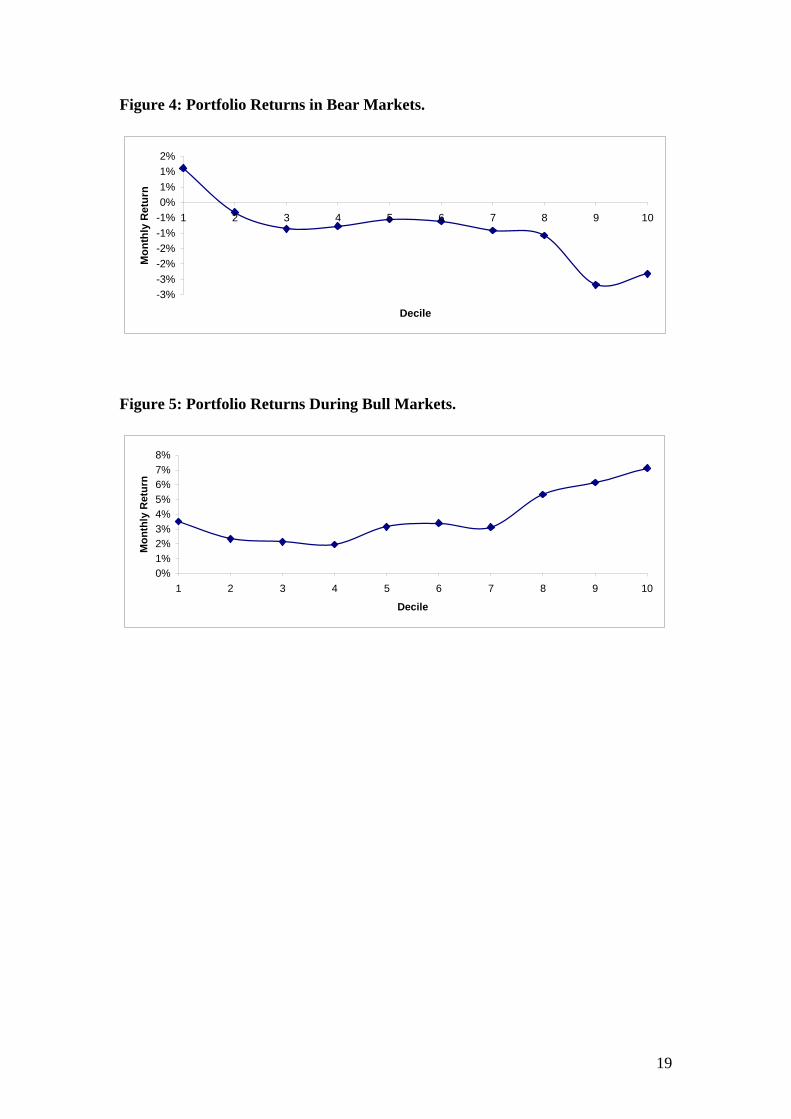
Figure 4: Portfolio Returns in Bear Markets.

-3%-3%-2%-2%-1%-1%0%1%1%2%

1 2 3 4 5 6 7 8 9 10

Decile

Mon

thly

Ret

urn

Figure 5: Portfolio Returns During Bull Markets.

0%1%2%3%4%5%6%7%8%

1 2 3 4 5 6 7 8 9 10

Decile

Mon

thly

Ret

urn

19

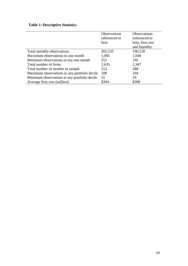
Table 1: Descriptive Statistics

Observations referenced to beta

Observations referenced to beta, firm size and liquidity

Total monthly observations 265,535 190,218 Maximum observations in one month 1,085 1,048 Minimum observations in any one month 552 192 Total number of firms 2,635 2,347 Total number of months in sample 312 288 Maximum observations in any portfolio decile 108 104 Minimum observations in any portfolio decile 55 19 Average firm size (million) $394 $398

20

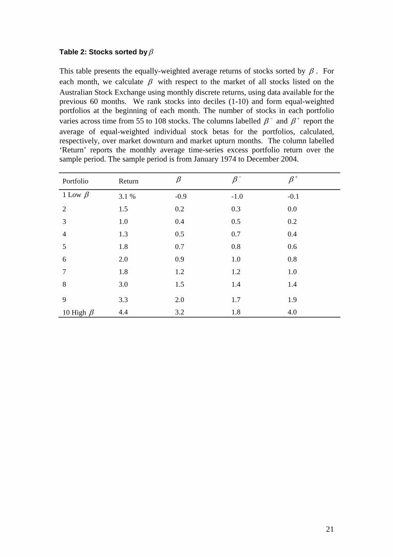
Table 2: Stocks sorted byβ

This table presents the equally-weighted average returns of stocks sorted by β . For each month, we calculate β with respect to the market of all stocks listed on the Australian Stock Exchange using monthly discrete returns, using data available for the previous 60 months. We rank stocks into deciles (1-10) and form equal-weighted portfolios at the beginning of each month. The number of stocks in each portfolio varies across time from 55 to 108 stocks. The columns labelled and report the average of equal-weighted individual stock betas for the portfolios, calculated, respectively, over market downturn and market upturn months. The column labelled ‘Return’ reports the monthly average time-series excess portfolio return over the sample period. The sample period is from January 1974 to December 2004.

−β +β

Portfolio Return β −β +β

1 Low β 3.1 % -0.9 -1.0 -0.1

2 1.5 0.2 0.3 0.0

3 1.0 0.4 0.5 0.2

4 1.3 0.5 0.7 0.4

5 1.8 0.7 0.8 0.6

6 2.0 0.9 1.0 0.8

7 1.8 1.2 1.2 1.0

8 3.0 1.5 1.4 1.4

9 3.3 2.0 1.7 1.9

10 High β 4.4 3.2 1.8 4.0

21

Table 3: Stocks sorted by −β

For each month, we calculate as for β in Table 2 and rank stocks into deciles (1-10) and form equal-weighted portfolios at the beginning of each month. The columns labelled

−β

β and report the time-series average of equal-weighted individual stock betas over the holding period for the portfolios formed on . The sample period is from January 1974 to December 2004.

+β−β

Portfolio −β β +β

1 Low −β -2.4 -0.05 1.0

2 -0.2 0.6 0.7

3 0.2 0.7 0.7

4 0.45 0.8 0.8

5 0.7 0.9 0.9

6 0.9 1.0 1.0

7 1.2 1.2 1.2

8 1.5 1.5 1.5

9 2.0 1.75 1.6 10 High −β 3.5 1.9 2.0

22

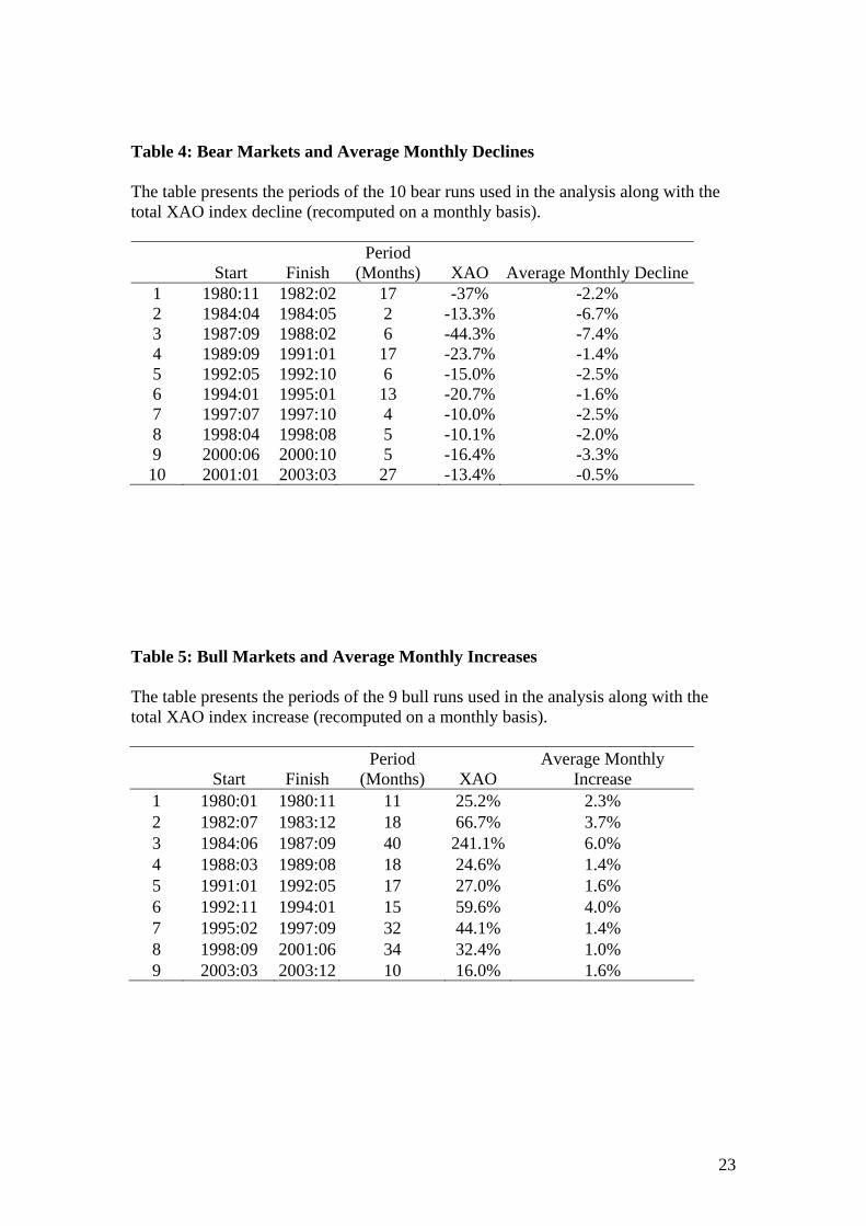
Table 4: Bear Markets and Average Monthly Declines

The table presents the periods of the 10 bear runs used in the analysis along with the total XAO index decline (recomputed on a monthly basis).

Start Finish Period

(Months) XAO Average Monthly Decline 1 1980:11 1982:02 17 -37% -2.2% 2 1984:04 1984:05 2 -13.3% -6.7% 3 1987:09 1988:02 6 -44.3% -7.4% 4 1989:09 1991:01 17 -23.7% -1.4% 5 1992:05 1992:10 6 -15.0% -2.5% 6 1994:01 1995:01 13 -20.7% -1.6% 7 1997:07 1997:10 4 -10.0% -2.5% 8 1998:04 1998:08 5 -10.1% -2.0% 9 2000:06 2000:10 5 -16.4% -3.3% 10 2001:01 2003:03 27 -13.4% -0.5%

Table 5: Bull Markets and Average Monthly Increases

The table presents the periods of the 9 bull runs used in the analysis along with the total XAO index increase (recomputed on a monthly basis).

Start Finish Period

(Months) XAO Average Monthly

Increase 1 1980:01 1980:11 11 25.2% 2.3% 2 1982:07 1983:12 18 66.7% 3.7% 3 1984:06 1987:09 40 241.1% 6.0% 4 1988:03 1989:08 18 24.6% 1.4% 5 1991:01 1992:05 17 27.0% 1.6% 6 1992:11 1994:01 15 59.6% 4.0% 7 1995:02 1997:09 32 44.1% 1.4% 8 1998:09 2001:06 34 32.4% 1.0% 9 2003:03 2003:12 10 16.0% 1.6%

23

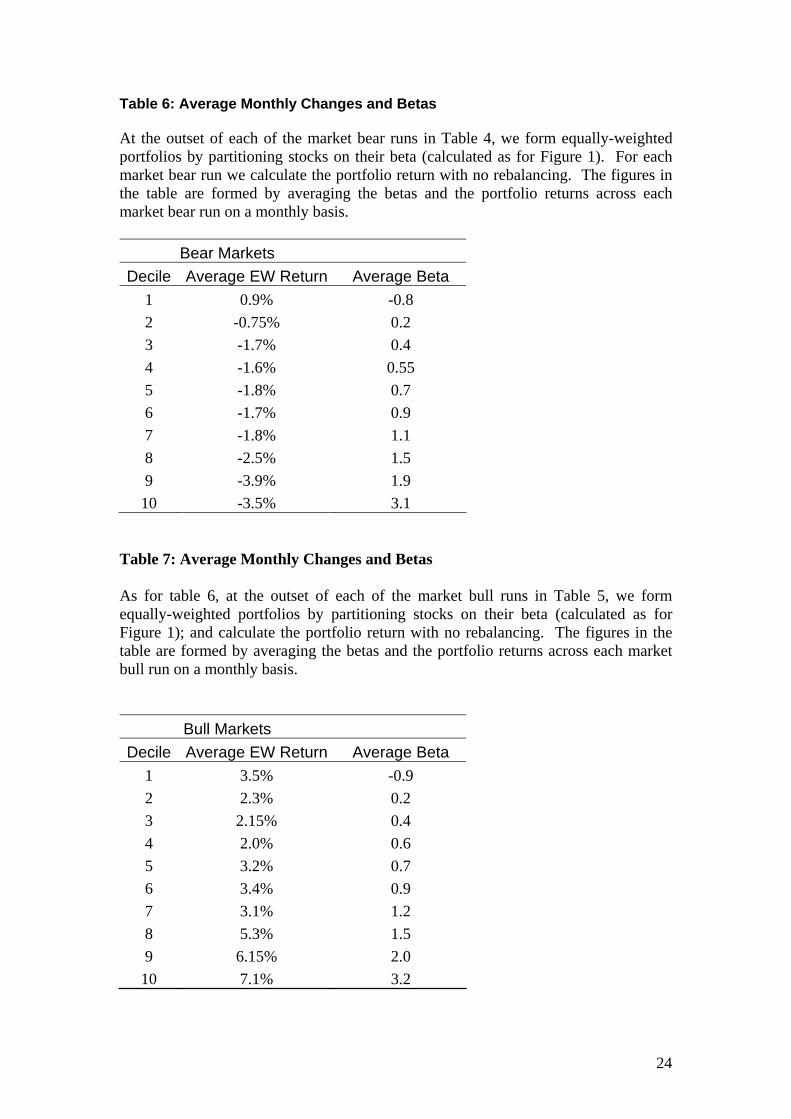
Table 6: Average Monthly Changes and Betas

At the outset of each of the market bear runs in Table 4, we form equally-weighted portfolios by partitioning stocks on their beta (calculated as for Figure 1). For each market bear run we calculate the portfolio return with no rebalancing. The figures in the table are formed by averaging the betas and the portfolio returns across each market bear run on a monthly basis.

Bear Markets Decile Average EW Return Average Beta

1 0.9% -0.8 2 -0.75% 0.2 3 -1.7% 0.4 4 -1.6% 0.55 5 -1.8% 0.7 6 -1.7% 0.9 7 -1.8% 1.1 8 -2.5% 1.5 9 -3.9% 1.9 10 -3.5% 3.1

Table 7: Average Monthly Changes and Betas As for table 6, at the outset of each of the market bull runs in Table 5, we form equally-weighted portfolios by partitioning stocks on their beta (calculated as for Figure 1); and calculate the portfolio return with no rebalancing. The figures in the table are formed by averaging the betas and the portfolio returns across each market bull run on a monthly basis.

Bull Markets Decile Average EW Return Average Beta

1 3.5% -0.9 2 2.3% 0.2 3 2.15% 0.4 4 2.0% 0.6 5 3.2% 0.7 6 3.4% 0.9 7 3.1% 1.2 8 5.3% 1.5 9 6.15% 2.0 10 7.1% 3.2

24

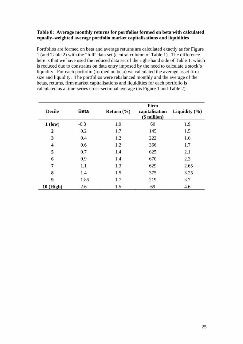
Table 8: Average monthly returns for portfolios formed on beta with calculated equally–weighted average portfolio market capitalisations and liquidities Portfolios are formed on beta and average returns are calculated exactly as for Figure 1 (and Table 2) with the “full” data set (central column of Table 1). The difference here is that we have used the reduced data set of the right-hand side of Table 1, which is reduced due to constrains on data entry imposed by the need to calculate a stock’s liquidity. For each portfolio (formed on beta) we calculated the average asset firm size and liquidity. The portfolios were rebalanced monthly and the average of the betas, returns, firm market capitalisations and liquidities for each portfolio is calculated as a time-series cross-sectional average (as Figure 1 and Table 2).

Decile Beta Return (%) Firm

capitalisation ($ million)

Liquidity (%)

1 (low) -0.3 1.9 60 1.9 2 0.2 1.7 145 1.5 3 0.4 1.2 222 1.6 4 0.6 1.2 366 1.7 5 0.7 1.4 625 2.1 6 0.9 1.4 670 2.3 7 1.1 1.3 629 2.65 8 1.4 1.5 375 3.25 9 1.85 1.7 219 3.7

10 (High) 2.6 1.5 69 4.6

25

Table 9

The average betas of stocks were partitioned as in the first row of the table. Within such partitions the average firm return, firm size, and liquidity are as presented in the final three rows. Return, firm size and liquidity characteristics for Australian stocks as a function of beta

Beta < 0.25 0.25 – 0.65 0.65 – 1.3 1.3 – 2.0 > 2.0

Annualised Return (%)

1.8 1.25 1.4 1.6 1.5

Size ( $ million)

< $150 $150 - $500 > $500 $150 - $500 < $150

Liquidity (monthly volume of trades to shares outstanding )

medium

2%

low

1.5%

medium

2.25%

medium-high

3.5%

high

4.5%

26