The Signaling Channel for Federal Reserve Bond Purchases · The Signaling Channel for Federal Reserve Bond Purchases. Michael D. Bauer Federal Reserve Bank of San Francisco . Glenn

FEDERAL RESERVE BANK OF SAN FRANCISCO

WORKING PAPER SERIES

The Signaling Channel for

Federal Reserve Bond Purchases

Michael D. Bauer Federal Reserve Bank of San Francisco

Glenn D. Rudebusch

Federal Reserve Bank of San Francisco

April 2013

The views in this paper are solely the responsibility of the authors and should not be interpreted as reflecting the views of the Federal Reserve Bank of San Francisco or the Board of Governors of the Federal Reserve System.

Working Paper 2011-21 http://www.frbsf.org/publications/economics/papers/2011/wp11-21bk.pdf

The Signaling Channel for

Federal Reserve Bond Purchases∗

Michael D. Bauer†, Glenn D. Rudebusch‡

April 3, 2013

Abstract

Previous research has emphasized the portfolio balance effects of Federal Reserve bond

purchases, in which a reduced bond supply lowers term premia. In contrast, we find that

such purchases have important signaling effects that lower expected future short-term

interest rates. Our evidence comes from a model-free analysis and from dynamic term

structure models that decompose declines in yields following Fed announcements into

changes in risk premia and expected short rates. To overcome problems in measuring

term premia, we consider bias-corrected model estimation and restricted risk price

estimation. In comparison with other studies, our estimates of signaling effects are

larger in magnitude and statistical significance.

Keywords: unconventional monetary policy, QE, LSAP, portfolio balance, no arbitrage

JEL Classifications: E43, E52

∗We thank for their helpful comments: Min Wei, Ken West, seminar participants at the Federal ReserveBank of Atlanta, Cheung Kong Graduate School of Business, the University of Wisconsin, and Santa ClaraUniversity, and conference participants at the 2011 CIMF/IESEG Conference in Cambridge, the 2011 SwissNational Bank Conference in Zurich, the 2012 System Macro Meeting at the Federal Reserve Bank of Cleve-land, the 2012 Conference of the Society for Computational Economics in Prague, the 2012 Meetings of theEuropean Economic Association in Malaga, the 2012 SoFiE Conference in Oxford, the Monetary EconomicsMeeting at the NBER 2012 Summer Institute, and the 2013 Federal Reserve Day-Ahead Conference in SanDiego. The views expressed herein are those of the authors and not necessarily shared by others at theFederal Reserve Bank of San Francisco or in the Federal Reserve System.

†Federal Reserve Bank of San Francisco, [email protected]‡Federal Reserve Bank of San Francisco, [email protected]

1 Introduction

During the recent financial crisis and ensuing deep recession, the Federal Reserve reduced its

target for the federal funds rate—the traditional tool of U.S. monetary policy—essentially to

the lower bound of zero. In the face of deteriorating economic conditions and with no scope

for further cuts in short-term interest rates, the Fed initiated an unprecedented expansion of

its balance sheet by purchasing large amounts of Treasury debt and federal agency securities

of medium and long maturities.1 Other central banks have taken broadly similar actions.

Notably, the Bank of England also purchased longer-term debt during the financial crisis,

and the Bank of Japan, when confronted over a decade ago with stagnation and near-zero

short-term rates, purchased debt securities in its program of Quantitative Easing (QE).2

The goal of the Fed’s large-scale asset purchases (LSAPs) was to put downward pressure

on longer-term yields in order to ease financial conditions and support economic growth. Us-

ing a variety of approaches, several studies have concluded that the Fed’s LSAP program was

effective in lowering various interest rates below levels that otherwise would have prevailed.3.

However, researchers do not yet fully understand the underlying mechanism and causes for

the declines in long-term interest rates. Based on the usual decomposition of yields on safe

long-term government bonds, there are two potential elements that central bank bond pur-

chases could affect: the term premium and the average level of short-term interest rates over

the maturity of the bond, also known as the risk-neutral rate. The term premium could have

fallen because the Fed’s LSAPs reduced the amount of longer-term bonds in private-sector

portfolios—which is loosely referred to as the portfolio balance channel. Alternatively, the

LSAP announcements could have led market participants to revise down their expectations

for future short-term interest rates, lengthening, for example, the expected period of a near-

zero federal funds rate target. Such a signaling channel for LSAPs would reduce yields by

lowering the average expected short-rate (or risk-neutral) component of long-term rates.

Much discussion of the financial market effects of the Fed’s bond purchases treats the

portfolio balance channel as the key channel for that impact. For example, Chairman Ben

Bernanke (2010) described the effects of the Fed’s bond purchases in this way:

I see the evidence as most favorable to the view that such purchases work pri-

marily through the so-called portfolio balance channel, which holds that once

short-term interest rates have reached zero, the Federal Reserve’s purchases of

1The federal agency securities were debt or mortgage-backed securities that had explicit or implicit creditprotection from the U.S. government.

2The Fed’s actions led to a larger central bank balance sheet and higher bank reserves much like the Bankof Japan’s QE; however, the Fed’s purchases were focused on longer-maturity assets.

3Among many others, see D’Amico and King (forthcoming), Gagnon et al. (2011), Hamilton and Wu(2012a), Krishnamurthy and Vissing-Jorgensen (2011), Neely (2012), and Woodford (2012).

1

longer-term securities affect financial conditions by changing the quantity and

mix of financial assets held by the public. Specifically, the Fed’s strategy relies

on the presumption that different financial assets are not perfect substitutes in

investors’ portfolios, so that changes in the net supply of an asset available to

investors affect its yield and those of broadly similar assets.

Along with central bank policy makers, researchers have also favored the portfolio balance

channel in accounting for the effects of LSAPs. The most influential evidence supporting a

portfolio balance channel has come from event studies that examine changes in asset prices

following announcements of central bank bond purchases. Notably, Gagnon et al. (2011),

henceforth GRRS, examine changes in the ten-year Treasury yield and Treasury yield term

premium.4 They document that after eight key LSAP announcements, the ten-year yield

fell by a total of 91 basis points (bps), while their measure of the ten-year term premium,

which is based on the model of Kim and Wright (2005), fell by 71 bps. Based largely on this

evidence, the authors argue that the Fed’s LSAPs primarily lowered long-term rates through

a portfolio balance channel that reduced term premia.

In this paper, we re-examine the notion that the signaling of lower future policy rates

through LSAP announcements played a negligible role in lowering Treasury yields. First,

we argue that the estimated declines in short rate expectations constitute a conservative

measure of the importance of the signaling channel because policy actions that signal lower

future short rates tend to lower term premia as well. Therefore, attributing changes in

term premia entirely to the portfolio balance channel is likely to underestimate the signaling

effects of LSAPs.

We also provide model-free evidence suggesting that the Fed’s actions lowered yields to

a considerable extent by changing policy expectations about the future path of the federal

funds rate. Under a market segmentation assumption that LSAPs primarily affected security-

specific term premia in Treasury markets, changes after LSAP announcements in spreads

between Treasury yields and money market and swap rates of comparable maturity illuminate

the contribution of the portfolio balance channel. Joyce et al. (2011), for example, argue that

increases in spreads between U.K. Treasury and swap yields following Bank of England QE

announcements support a portfolio balance channel. In contrast, in the United States, we find

that a large portion of the observed yield changes was also reflected in lower money market

and swap rates. This suggests that the expectations component may make an important

contribution to the declines in yields.

Our main contribution is to provide new model-based evidence that addresses two key sta-

4Other event studies include Joyce et al. (2011), Neely (2012), Krishnamurthy and Vissing-Jorgensen(2011), and Swanson (2011).

2

tistical problems in decomposing the yield curve in previous studies—namely, small-sample

bias and statistical uncertainty. We reconsider the GRRS results that are based on the Kim-

Wright decompositions of yields into term premia and risk-neutral rates using a conventional

arbitrage-free dynamic term structure model (DTSM). Although DTSMs are the workhorse

model in empirical fixed income finance, they have been very difficult to estimate and are

plagued by biased coefficient estimates as described by previous studies—see, for example,

Duffee and Stanton (2012), Kim and Orphanides (2012), and Bauer et al. (2012), henceforth

BRW. Therefore, to get better measures of the term premium, we examine two alternative

estimates of the DTSM. The first is obtained from a novel estimation procedure—following

BRW—that directly adjusts for the small-sample bias in estimation of a maximally flexible

DTSM. Since conventional biased DTSM estimates—like the Kim-Wright model that GRRS

rely on—overstate the speed of mean reversion of the short rate, the model-implied forecast

of the short rate is too close to the unconditional mean. Consequently, too much of the

variation in forward rates is attributed to the term premium component. Intuitively then,

conventional biased DTSM estimates understate the importance of the signaling channel.

Indeed, we find that an LSAP event study using term premia obtained from DTSM esti-

mates with reduced bias finds a larger role for the signaling channel. Our second estimation

approach imposes restrictions on the risk pricing as in Bauer (2011). Intuitively, under re-

stricted risk pricing, the cross-sectional interest rate dynamics, which are estimated very

precisely, pin down the time series parameters. This reduces both small-sample bias and

statistical uncertainty, so that short rate forecasts and term premium estimates are more

reliable (Cochrane and Piazzesi, 2008; Joslin et al., 2012; Bauer, 2011). Here, too, we find a

more substantial role for the signaling channel than is commonly acknowledged.

Thus, the use of alternative term structure models appears to lead to different conclusions

about the relative importance of expectations and term premia in accounting for interest rate

changes following LSAP announcements. To conduct a full-scale evaluation of a wide range

of models using out-of-sample forecasting and other criteria is beyond the scope of this paper.

However, our selected models have a solid foundation including the Monte Carlo evidence in

BRW that shows the importance of bias correction to infer interest rate dynamics. In par-

ticular, our models address the serious concern that conventional DTSMs lead to short rate

expectations that are implausibly stable—voiced, among others, by Piazzesi and Schneider

(2011) and Kim and Orphanides (2012)—in a couple of different ways. The implication is

that the greater impotance of the signaling channel is likely to be robust to alternative

specifications that take this concern seriously.5

5The inclusion of survey forecasts in the Kim-Wright estimates is motivated in part to address justthis concern, but our evidence—and the more-detailed examination by Christensen and Rudebusch (2012)—

3

Importantly, we quantify the statistical uncertainty surrounding the DTSM-based es-

timates of the relative contributions of the portfolio balance and signaling channels. In

particular, we take into account the parameter uncertainty that underlies estimates of the

term premium and produce confidence intervals that reflect this estimation uncertainty. Our

confidence intervals reveal that with a largely unrestricted DTSM, as is common in the

literature, definitive conclusions about the relative importance of term premia and expec-

tations effects of LSAPs are difficult. For the results based on unrestricted DTSMs, both

of the extreme views of “only term premia” and “only expectations” effects are statisti-

cally plausible. However, under restrictions on the risk pricing in the DTSM, statistical

uncertainty is reduced. Consequently, our decompositions of the LSAP effects using DTSM

estimates under restricted risk prices not only point to a larger role of the signaling channel,

but also allow much more precise inference about the respective contribution of signaling

and portfolio balance. Taken together, our results indicate that an important effect of the

LSAP announcements was to lower the market’s expectation of the future policy path, or,

equivalently, to lengthen the expected duration of near-zero policy rates.

There is a burgeoning literature assessing the effects of the Fed’s asset purchases. Our

results pointing to economically and statistically significant role for the signaling channel

are quantitatively and qualitatively different from those in GRRS. There are three no-

table papers that also provide evidence in favor of signaling effects of the Fed’s LSAPs.

Krishnamurthy and Vissing-Jorgensen (2011), henceforth KVJ, consider changes in money

market futures rates and conclude that signaling likely was an important channel for LSAP

effects on both safe and risky assets. In subsequent work, Woodford (2012) emphasizes

the strong theoretical assumptions necessary to give rise to portfolio balance effects, and

presents very different model-free empirical evidence for a strong signaling channel, partly

drawing upon the analysis in Campell et al. (2012). Our model-free results parallel the

evidence in those papers, based on similar auxiliary assumptions, while our model-based

analysis substantially extends their analysis and provides formal statistical evidence for

the importance of the signaling channel. Finally, again subsequent to our initial work,

Christensen and Rudebusch (2012) also provide a model-based event study using a different

set of DTSM specifications that contrasts the effects of the Fed’s and the Bank of England’s

asset purchase programs. Interestingly, their results suggest that the relative contribution

of the portfolio balance and signaling channels seems to depend on the forward guidance

communication strategy pursued by the central bank and the institutional depth of financial

markets.

suggest that the contribution of expectations to daily changes in long-term interest rates is still understatedby the resulting estimates.

4

The paper is structured as follows. In Section 2, we describe the portfolio balance and

signaling channels for LSAP effects on yields and discuss the event study methodology that

we use to estimate the effects of the LSAPs. Section 3 presents model-free evidence on

the importance of the signaling and portfolio balance channels. Section 4 describes the

econometric problems with existing term premium estimates and outlines our two approaches

for obtaining more appropriate decompositions of long rates. In Section 5, we present our

model-based event study results. Section 6 concludes.

2 Identifying portfolio balance and signaling channels

Here we describe the two key channels through which LSAPs can affect interest rates and

discuss how their respective importance can be quantified, albeit imperfectly, through an

event study methodology.

2.1 Portfolio balance channel

In the standard asset-pricing model, changes in the supply of long-term bonds do not affect

bond prices. In particular, in a pricing model without frictions, bond premia are determined

by the risk characteristics of bonds and the risk aversion of investors, both of which are

unaffected by the quantity of bonds available to investors. In contrast, to explain the response

of bond yields to central bank purchases of bonds, researchers have focused their attention

exactly on the effect that a reduction in bond supply has on the risk premium that investors

require for holding those securities. The key avenue proposed for this effect is the portfolio

balance channel.6 As described by GRRS:

By purchasing a particular asset, a central bank reduces the amount of the se-

curity that the private sector holds, displacing some investors and reducing the

holdings of others, while simultaneously increasing the amount of short-term,

risk-free bank reserves held by the private sector. In order for investors to be

willing to make those adjustments, the expected return on the purchased security

has to fall. (p. 6)

The crucial departure from a frictionless model for the operation of a portfolio balance

channel is that bonds of different maturities are not perfect substitutes. Instead, risk-averse

6Like most of the literature, we focus on the portfolio balance channel to account for term premia effectsof LSAPs. Some recent papers have also discussed a market functioning channel through which LSAPs couldaffect bond premia, including, for example, GRRS, KVJ, and Joyce et al. (2010). This channel would seemmost relevant for limited periods of dislocation in markets for securities other than Treasuries.

5

arbitrageurs are limited in the market and there are “preferred-habitat” investors who have

maturity-specific bond demands.7 In this setting, the maturity structure of outstanding debt

can affect term premia.

The precise portfolio balance effect of purchases on term premia in different markets

will vary depending on the interconnectedness of markets. To be concrete, consider the

decomposition of the ten-year Treasury yield, y10t , into a risk-neutral component,8 Y RN10t ,

and a term premium, Y TP 10t :

y10t = Y RN10t + Y TP 10

t (1)

= Y RN10t + Y TP 10

risk,t + Y TP 10instrument,t. (2)

The term premium is further decomposed in equation (2) into a maturity-specific term pre-

mium, Y TP 10risk,t, that reflects the pricing of interest risk and an idiosyncratic instrument-

specific term premium, Y TP 10instrument,t, that captures, for example, demand and supply im-

balances for that particular security.9

In analyzing the portfolio balance channel, some researchers have emphasized market

segmentation between securities of different maturities, as in the formal preferred-habitat

model, or between different fixed income securities with similar risk characteristics. Specif-

ically, market segmentation between the government bond markets and other fixed income

markets could reflect the specific needs of pension funds, other institutional investors, and

foreign central banks to hold safe government bonds, and arbitrageurs that are institution-

ally constrained or simply too small in comparison to such huge demand flows. Changes in

the bond supply then would have direct price effects through Y TP 10instrument,t on the securities

that were purchased, and the magnitude of the price change would depend on how much

of that security was purchased. The effects on securities that were not purchased would be

small. Notably, for the U.K., Joyce et al. (2011) find that the price effects on those securi-

ties purchased by the Bank of England were much larger than for other securities that were

not purchased (e.g., swap contracts), which points to significant market segmentation. This

version of the portfolio balance channel can be termed a local supply channel.

7Recent work on the theoretical underpinnings of the portfolio balance channel includes Vayanos and Vila(2009) and Hamilton and Wu (2012a).

8The risk-neutral yield equals the expected average risk-free rate over the lifetime of the bond under thereal-world, or P, probability measure (plus a negligible convexity term). The risk-neutral yield is the interestrate that would prevail if all investors were risk neutral. It is not calculated under the risk-neutral, or Q,probability measure.

9Also, the safety premium discussed by KVJ would be in this final term, as noted by D’Amico et al.(2012).

6

Alternatively, markets for securities may be somewhat connected because of the presence

of arbitrageurs. For example, GRRS have emphasized the case of investors that prefer a

specific amount of duration risk along with a lack of maturity-indifferent arbitrageurs with

sufficiently deep pockets. In this case, changes in the bond supply affect the aggregate

amount of duration available in the market and the pricing of the associated interest rate

risk term premia, Y TP 10risk,t. In this duration channel, central bank purchases of even a few

specific bonds can affect the risk pricing and term premia for a wide range of securities.

Notably, in the absence of further frictions, all fixed income securities (e.g., swaps and

Treasuries) of the same duration would be similarly affected. Furthermore, if the Fed were

to remove a given amount of duration risk from the market by purchasing ten-year securities

or by purchasing (a smaller amount of) 30-year securities, the effect through the duration

channel would be the same.

Thus, there are two ways in which bond purchases can directly affect term premia in

Treasury yields through portfolio balance effects: First, if markets for Treasuries and other

assets (including Treasuries of varying maturity) are segmented, bond purchases can reduce

Treasury-specific (or maturity-specific) premia (local supply channel). Second, by lowering

aggregate duration risk, purchases can reduce term premia in all fixed-income securities

(duration channel).

2.2 Signaling channel

The portfolio balance channel, which emphasizes the role of quantities of securities in asset

pricing, runs counter to at least the past half century of mainstream frictionless finance

theory. That theory, which is based on the presence of pervasive, deep-pocketed arbitrageurs,

has no role for financial market segmentation or movements in idiosyncratic, security-specific

term premia like Y TP 10instrument,t. Moreover, the duration channel and its associated shifts in

Y TP 10risk,t would also be ignored in conventional models. In particular, the scale of the Fed’s

LSAP program—$1.725 trillion of debt securities—is arguably small relative to the size of

bond portfolios. The U.S. fixed income market is on the order of $30 trillion, and the global

bond market—arguably, the relevant one—is several times larger. In addition, other assets,

such as equities, also bear duration risk.

Instead, the traditional finance view of the Fed’s actions would focus on the new infor-

mation provided to investors about the future path of short-term interest rates, that is, the

potential signaling channel for central bank bond purchases to affect bond yields by changing

the risk-neutral component of interest rates. In general, LSAP announcements may signal

to market participants that the central bank has changed its views on current or future eco-

7

nomic conditions. Alternatively, they may be thought to convey information about changes

in the monetary policy reaction function or policy objectives, such as the inflation target. In

such cases, investors may alter their expectations of the future path of the policy rate, per-

haps by lengthening the expected period of near-zero short-term interest rates. According to

such a signaling channel, announcements of LSAPs would lower the expectations component

of long-term yields. In particular, throughout 2009 and 2010, investors were wondering how

long the Fed would leave its policy interest rate unchanged at essentially zero. The language

in the various FOMC statements in 2009 that economic conditions were ”likely to warrant

exceptionally low levels of the federal funds rate for an extended period,” provided some

guidance, but the zero bound was terra incognita. In such a situation, the Fed’s unprece-

dented announcements of asset purchases with the goal of putting further downward pressure

on yields might well have had an important signaling component, in the sense of conveying

to market participants how bad the economic situation really was, and that extraordinarily

easy monetary policy was going to remain in place for some time.

2.3 Event study methodology

The few studies to consider the relative contributions of the portfolio balance and signaling

channels, specifically GRRS and KVJ for the U.S. and Joyce et al. (2011) for the U.K., have

used an event study methodology.10 This methodology focuses on changes in asset prices

over tight windows around discrete events. We also employ such a methodology to assess

the effects of LSAPs on fixed income markets.

In the portfolio balance channel described above, it is the quantity of asset purchases

that affects prices; however, forward-looking investors will in fact react to news of future

purchases. Therefore, because changes in the expected maturity structure of outstanding

bonds are priced in immediately, credible announcements of future LSAPs can have the

immediate effect of lowering the term premium component of long-term yields. In our event

study, we focus on the eight LSAP announcements that GRRS include in their baseline event

set, which are described in Table 1.

In calculating the yield responses to these announcements, there are two competing re-

quirements for the size of the event window so that price changes reflect the effects of the

announcements. First, the window should be large enough to encompass all of an announce-

ment’s effects. Second, the window should be short enough to exclude other events that

10GRRS also provide evidence on the portfolio balance channel from monthly time-series regressions ofthe Kim-Wright term premium on variables capturing macroeconomic conditions and aggregate uncertainty,as well as a measure of the supply of long-term Treasury securities. However, our experience with theseregressions suggests the results are sensitive to specification (see also Rudebusch, 2007).

8

might significantly affect asset prices. Following GRRS, we use one-day changes in mar-

ket rates to estimate responses to the Fed’s LSAP announcements.11 A one-day window

appears to be a workable compromise. First, for large, highly liquid markets such as the

Treasury bond market, and under the assumption of rational expectations, new informa-

tion in the announcement about economic fundamentals should quickly be reflected in asset

prices. Second, the LSAP announcements appear to be the dominant sources of news for

fixed income markets on the days under consideration. On these announcement days, the

majority of bond and money market movements appeared to be due to new information that

markets received about the Fed’s LSAP program.

On two of the LSAP event dates, the FOMC press release also contained direct statements

about the path for the federal funds rate. On December 16, 2008, the FOMC decreased the

target for the policy rate to a range from 0 to 1/4 percent, and indicated that it expected

the target to remain there “for some time.” On March 18, 2009, the FOMC changed the

language about the expected duration of a near-zero policy rate to “for an extended period.”

Hence there were some conventional monetary policy actions, taking place at the same time

as LSAP announcements. Our analysis will not be able to distinguish this direct signaling

from the signaling effects through the LSAP announcements themselves. However, leaving

out these two dates from our event study analysis in fact increases the estimated relative

contribution of the expectations component to the yield declines (see discussion below of

Tables 6 and 7). Hence our empirical analysis is robust to this caveat.

Of course, if news about LSAPs is leaked or inferred prior to the official announcements,

then the event study will underestimate the full effect of the LSAPs. The inability to

account for important pre-announcement LSAP news makes us wary of analyzing later LSAP

announcements after the eight examined. For example, expectations of a second round of

asset purchases (QE2) were incrementally formed before official confirmation in fall 2010,

which is a possible reason for why studies like KVJ find small effects on financial markets

in their event study of QE2. For the events we consider, one can argue that markets mostly

did not expect the Fed’s purchases ahead of the announcements.12

2.4 Changes in risk-neutral rates and the role of signaling

How can an event study can distinguish between the portfolio balance and signaling channels?

A simple conventional view would associate these two channels, respectively, with changes

in term premia and risk neutral rates following LSAP announcements. However, there is

11Our results are robust to using the two-day change following announcements.12On the issue of the surprise component of monetary policy announcements during the recent LSAP

period see Wright (2011) and Rosa (2012).

9

an important complication in this empirical assessment: As a theoretical matter, the split

between the portfolio balance and signaling channels is not the same as the decomposition

of the long rate into expectations and risk premium components. In fact, because of second-

round effects of the portfolio balance and signaling channels, estimated changes of risk-

neutral rates are likely a lower bound for the contribution of signaling to changes in long-term

interest rates.

To illustrate the mapping between the two channels and the long rate decomposition,

first consider a scenario with just a portfolio balance channel and no signaling. In this case,

LSAPs reduce term premia, which would act to boost future economic growth.13 However,

the improved economic outlook will also reduce the amount of conventional monetary policy

stimulus needed because to achieve the optimal stance of monetary policy, the more policy-

makers add of one type of stimulus, the less they need to add of another. Thus, the operation

of a portfolio balance channel would cause LSAPs to increase risk-neutral rates as well as

reducing the term premium. In this case, we would measure higher policy expectations de-

spite the absence of any direct signaling effects. The changes in risk-neutral rates following

LSAP announcements will include both the direct signaling effects (presumably negative), as

well as the indirect portfolio balance effects on future policy expectations (positive). Hence,

this would mean that the true signaling effects on risk-neutral rates are likely larger than

the estimated decreases in risk-neutral rates.

Conversely, consider the case with no portfolio balance effects but a signaling channel that

operates because LSAP announcements contain news about easier monetary policy in the fu-

ture. This news could take various forms, such as, (1) a longer period of near-zero policy rate,

(2) lower risks around a little-changed but more certain policy path, (3) higher medium-term

inflation and potentially lower real short-term interest rates, and (4) improved prospects for

real activity, including diminished prospects for Depression-like outcomes. Taken together,

it seems likely that this news, and the demonstration of the Fed’s commitment to act, would

reduce the likelihood of future large drops in asset prices and hence lower the risk premia on

financial assets. Indeed, although the effects of easier expected monetary policy on term pre-

mia could in general go either way, during the previous Fed easing cycle from 2001 to 2003,

lower risk-neutral rates were accompanied by lower term premia. Table 2 shows changes

in the actual, fitted, and risk-neutral ten-year yield, and in the corresponding yield term

premium (according to the Kim-Wright model) for those days with FOMC announcements

during 2001 to 2003 when the risk-neutral rate decreased.14 That is, on days on which the av-

13On this connection, see Rudebusch et al. (2007).14The data for actual (fitted) yields and the Kim-Wright decomposition of yields are both available at

http://www.federalreserve.gov/econresdata/researchdata.htm (accessed August 30, 2011). Similar qualita-tive conclusions are obtained when we use our preferred term premium measures described later.

10

erage expected future policy rate was revised downward by market participants—comparable

to the potential signaling effects of LSAP announcements—the term premium usually fell as

well. Over all such days, the cumulative change in the term premium was -21 bps, which has

the same sign and more than half the magnitude of the cumulative change in the risk-neutral

yield (-35 bps). Thus, during this episode, easing actions that lowered policy expectations

at the same time lowered term premia. Arguably, the signaling effect of LSAPs on term

premia would be even larger in the recent episode given the potential curtailment of extreme

downside risk.

Both of these second-round effects work in the same direction of making the decomposi-

tion into changes in risk-neutral rates and term premia a downwardly biased estimate for the

importance of the signaling channel. Therefore, the event study results should be considered

conservative ones, with the true signaling effects likely larger than the estimated decreases

in risk-neutral rates.

3 Model-free evidence

One possible approach to evaluate how an LSAP program affected financial markets is to

consider model-free event-study evidence. A prominent example is the study by KVJ which

attempts to disentangle different channels of LSAPs exclusively by studying different market

rates, without using a model. In this section we do the same, focusing on just the portfolio

balance and signaling channels. We use interest rate data on money market futures, overnight

index swaps (OIS), and Treasury securities.

What can we learn about changes in policy expectations and risk premia from considering

such interest rates without a formal model? Of course, these interest rates also contain a

term premium and thus do not purely reflect the market’s expectations of future short rates.

Hence we need auxiliary assumptions, and there are two kinds of plausible assumptions in

this context. First, at short maturities, the term premium is likely small, because short-term

investments do not have much duration risk. Thus, changes in near-term rates are plausibly

driven by the expectations component. This argument can be used to interpret changes at

the very short end of the term structure of interest rates, such as movements in near-term

money market futures rates (see below) or in short-term yields (see, for example, GRRS,

p. 24). Second, we can make assumptions related to market segmentation, which we now

discuss in more detail.

11

3.1 Market segmentation

If markets are segmented to the extent that the portfolio balance effects of LSAPs operate

mainly through the local supply channel, and consequently on instrument-specific premia,

Y TP ninstrument,t, then the responses of futures and OIS rates mainly reflect the signaling

effects of the announcements. Specifically, changes in the spreads between these interest

rates and the rates on the purchased securities reflect portfolio balance effects on yield-

specific term premia. For example, Joyce et al. (2011) assume that the Bank of England’s

asset purchases only affect the term premium specific to gilts and neither the instrument-

specific term premium in OIS rates (which were not part of the asset purchases) nor the

general level of the term premium, Y TP nrisk,t. This market segmentation assumption enables

them to draw inferences about the importance of signaling and portfolio balance purely

from observed interest rates in OIS and bond markets: Movements in OIS rates reflect

signaling effects, and movements in yield-OIS spreads reflect portfolio balance effects. They

find that the responses of spreads are large, accounting for the majority of the responses of

yields. This points to an important role for the portfolio balance channel in the U.K. It also

indicates that the market segmentation assumption is plausible in their context, because the

signaling or duration channels could not explain the differential effects on rates with similar

risk characteristics.

Here we produce evidence similar to that of Joyce et al. (2011) for the U.S., considering

both money market futures and OIS rates. We do not claim that the market segmenta-

tion assumption is entirely plausible for the Treasury and OIS/futures markets, since these

securities are close substitutes. To a reader that questions the effects on duration risk com-

pensation and prefers the local supply story, the results below will be evidence about the

importance of signaling and portfolio balance effects. More generally though, without the

identifying assumption that changes in Y TP nrisk,t are negligible, the changes in the spreads

reflect changes in both Y RNnt and Y TP n

risk,t, and thus constitute an upper bound for the

magnitude of shifts in policy expectations.

3.2 Money market futures

Money market futures are bets on the future value of a short-term interest rate, and they

are used by policymakers, academics, and practitioners to construct implied paths for future

policy rates. Federal funds futures settle based on the federal funds rate, and contracts for

maturities out to about six months are highly liquid. Eurodollar futures pay off according

to the three-month London interbank offered rate (LBOR), and the most liquid contracts

have quarterly maturities out to about four years. While LBOR and the fed funds rate

12

do not always move in lockstep, these two types of futures contracts are typically used in

combination to construct a policy path over all available horizons.

How has the futures-implied policy path has changed around LSAP dates? Figure 1 shows

the futures-implied policy paths around the first five LSAP events, based on futures rates on

the end of the previous day and on the end of the event day.15 On almost all days, the policy

paths appear to have shifted down significantly at horizons of one year and longer in response

to the LSAP announcements.16 Table 3 displays the changes at specific horizons on all eight

LSAP event days. Also shown are total changes over all event days, as well as cumulative

changes and standard deviations of daily changes over the LSAP period. At the short end,

the path has shifted down by about 20-40 bps, while at longer horizons of one to three years

the total decrease is around 50 bps. Because the decreases in short-term futures rates are

arguably driven primarily by expectations, these results indicate that markets revised their

near-term policy expectations downward around LSAP announcements by about 20-40 bps.17

Note that this analysis is parallel to KVJ’s assessment of the importance of the signaling

channel.

What about policy expectations at longer horizons? The last three columns of the table

show the changes in the average futures-implied policy path over the next three years, the

changes in the three-year yield, and the spread between the yield and the futures-implied

rate.18 The futures-implied three-year yield declined by 43 bps, which corresponds to 54

percent of the decline in the yield. With the exception of March 2009, every LSAP an-

nouncement had a much larger effect on the futures-implied yield than on the Treasury

yield. Under a market segmentation assumption, this evidence suggests that lower policy

expectations accounted for more than half of the decrease in the three-year yield.

15The policy paths are derived using federal funds futures contracts for the current quarter and two quartersbeyond that. For longer horizons, we use Eurodollar futures, which are adjusted by the difference betweenthe last quarter of the federal funds futures contracts and the overlapping Eurodollar contract. Beginningfive months out, a constant term premium adjustment of 1bp per month of additional maturity is applied.

16The FOMC statement for January 28, 2009, contrary to the other announcements, actually causedsizable increases in yields and other market interest rates, as documented in GRRS and in our results below.Anecdotal evidence indicates that market participants were disappointed by the lack of concrete languageregarding the possibility and timing of purchases of longer-dated Treasury securities.

17One minor confounding factor is that on December 16, 2008, markets also were surprised by the targetrate decision—expectations were for a new target of 25 bps, however the Federal Open Market Committeedecided on a target range of 0-25 bps. Changes in short-term rates on this day reflect also reflect the effectsof conventional monetary policy.

18Yields are zero-coupon yields from a smoothed yield curve data set constructed in Gurkaynak et al.(2007). See http://www.federalreserve.gov/econresdata/researchdata.htm (accessed July 29, 2011).

13

3.3 Overnight index swaps

In an overnight index swap (OIS), one party pays a fixed interest rate on the notional amount

and receives the overnight rate, i.e., the federal funds rate, over the entire maturity period.

Under absence of arbitrage, OIS rates reflect risk-adjusted expectations of the average policy

rate over the horizon corresponding to the maturity of the swap. Intuitively, while futures

are bets on the value of the short rate at a future point in time, OIS contracts are essentially

bets on the average value of the short rate over a certain horizon.

Table 4 shows the results of an event study analysis of changes in OIS rates with matu-

rities of two, five, and ten years, yields of the same maturities, and yield-OIS spreads. We

consider the same set of event dates as before.19 The responses of yields to the Fed’s LSAP

announcements are similar to the responses of OIS rates. For certain days and maturities,

OIS rates respond even more strongly than yields, and at the ten-year maturity, the cumu-

lative change of the OIS rate is larger than the yield change, which results in an increasing

OIS spread. In those instances where the OIS spread significantly decreased, its relative

contribution to the yield change is typically still much smaller than the contribution of the

OIS rate change. The March 2009 announcement is the only one that significantly lowered

spreads. On the other event days, yield-OIS spreads barely moved or increased, suggesting

that large decreases in term premia are unlikely.

Clearly, yields and OIS rates moved very much in tandem in response to the LSAPs. Our

evidence in this section is consistent with the finding of GRRS “that LSAPs had widespread

effects, beyond those on the securities targeted for purchase” (p. 20). Under a market seg-

mentation identifying assumption, the evidence that OIS rates showed pronounced responses

suggests an important contribution of lower policy expectations to the decreases in inter-

est rates. Without such an assumption, it just indicates that instrument-specific premia in

Treasuries did not move much around announcements.

Some readers might find our result unsurprising: Safe government bonds and swap con-

tracts have similar risk characteristics, are likely to be close substitutes, and could therefore

be expected a priori to respond similarly to policy actions. This of course simply amounts

to not accepting the market segmentation assumption for these securities. However, there

are two important points to keep in mind in response to this critique: First, the evidence

for the U.K. has shown that yields and OIS rates do not necessarily need to respond simi-

larly. For the case of the U.K., these instruments are not very close substitutes and there

is considerable market segmentation, thus one might be inclined to find this plausible for

the U.S. as well. Second, the same results hold for securities that are less close substitutes.

19OIS rates are taken from Bloomberg.

14

Specifically, the evidence in KVJ as well as our own calculations using different data sources

(results omitted) show that highly-rated corporate bonds responded about as much as Trea-

sury yields to LSAPs.20 Clearly a Treasury bond and, say, a AA-rated corporate bond are

not close substitutes, thus market segmentation is more plausible, and the fact that they

respond in tandem is evidence that signaling played an important role.

However plausible one finds the necessary auxiliary assumptions, model-free analysis can

only go so far. Thus, we now turn to model-based evidence to address whether Treasuries

were affected by the LSAPs through downward shifts in the expected policy path and through

shifts in a their term premium.

4 Term premium estimation

A theoretically rigorous decomposition of interest rates into expectations and term premium

components requires a DTSM, which have generally proven difficult to estimate. Therefore,

we consider several different model estimates to ensure robustness.

4.1 Econometric problems: bias and uncertainty

To estimate the term premium component in long-term interest rates, researchers typically

resort to DTSMs. Such models simultaneously capture the cross section and time series

dynamics of interest rates, and impose absence of arbitrage, which ensures that the two

are consistent with each other. Term premium estimates are obtained by forecasting the

short rate using the estimated time series model, and subtracting the average short rate

forecast (i.e., the risk-neutral rate) from the actual interest rate. The very high persistence of

interest rates, however, causes major problems with estimating the time series dynamics. The

parameter estimates typically suffer from small-sample bias and large statistical uncertainty,

which makes the resulting estimated risk-neutral rates and term premia inherently unreliable.

The small-sample bias in conventional estimates of DTSMs stems from the fact that the

largest root in autoregressive models for persistent time series is generally underestimated.

Therefore the speed of mean reversion is overestimated, and the model-implied forecasts for

longer horizons are too close to the unconditional mean of the process. Consequently, risk-

neutral rates are too stable, and too much of the variation in long-term rates is attributed

to the term premium component.21 In the context of LSAP event studies, this bias works

20Changes in default-risk premia do not account for this response, based on KVJ’s evidence that incorpo-rates credit default swap data.

21 This problem has been pointed out by Ball and Torous (1996) and discussed in subsequent studiesincluding BRW.

15

in the direction of attributing too large a share of changes in long-term interest rates to

the term premium. Hence, the relative importance of the portfolio balance channel will be

overestimated. Because of this concern, we conduct an event study using term premium

estimates that correct for this bias.

Large statistical uncertainty underlies any estimate of the term premium, due to both

specification and estimation uncertainty. The former reflects uncertainty about different

plausible specifications of a DTSM, which might lead to quite different economic implica-

tions.22 We address this issue in a pragmatic way by presenting alternative estimates based

on different specifications. Estimation uncertainty exists because the parameters governing

the time series dynamics in a DTSM are estimated imprecisely, due to the high persistence

of interest rates.23 Consequently, large statistical uncertainty underlies short rate forecasts

and term premia calculated from such parameter estimates. Despite this fact, studies typ-

ically report only point estimates of term premia.24 In our event study, we report interval

estimates of changes in risk-neutral rates and of changes in the term premium.

4.2 Alternative term premium estimates

We now briefly describe the alternative term premium estimates that we include in our event

study. Details are provided in appendices. The data used in the estimation of our models

consist of daily observations of interest rates from January 2, 1985, to December 30, 2009.

We include T-bill rates at maturities of 3 and 6 months from the Federal Reserve H.15 release

and zero-coupon yields at maturities of 1, 2, 3, 5, 7, and 10 years.

4.2.1 Kim-Wright

The term premium estimates used by GRRS are obtained from the model of Kim and Wright

(2005). What distinguishes their model from an unrestricted, i.e., maximally flexible, affine

Gaussian DTSM is the inclusion of survey-based short rate forecasts and some slight re-

strictions on the risk pricing. While Kim and Orphanides (2012) argue that incorporating

additional information from surveys might help alleviate the problems with DTSM esti-

mation, it is unclear to what extent bias and uncertainty are reduced. Survey expecta-

tions are problematic because on the one hand they are available only at low frequencies

(monthly/quarterly), and on the other hand they might not represent rational forecasts of

22This issue has been highlighted, for example, by Rudebusch et al. (2007) and Bauer (2011).23The slow speed of mean reversion of interest rates makes it difficult to pin down the unconditional mean

and the persistence of the estimated process. See, among others, Kim and Orphanides (2012).24Exceptions are the studies by Bauer (2011) and Joslin et al. (2012), who present measures of statistical

uncertainty around estimated risk-neutral rates and term premia.

16

short rates (Piazzesi and Schneider, 2008). In terms of risk price restrictions, the model

imposes only very few constraints, so the link between cross-sectional dynamics and time

series dynamics is likely to be weak.

4.2.2 Ordinary least squares

As a benchmark, we estimate a maximally-flexible affine Gaussian DTSM. The risk factors

correspond to the first three principal components of yields. We use the normalization of

Joslin et al. (2011). The estimation is a two-step procedure: First, the parameters of the

vector autoregression (VAR) for the risk factors are estimated using ordinary least squares

(OLS). Second, we obtain estimates of the parameters governing the cross-sectional dynamics

using the minimum-chi-square method of Hamilton and Wu (2012b). Because the model is

exactly identified, these are also the maximum likelihood (ML) estimates. Details on the

estimation can be found in Appendix B.1.

To account for the estimation uncertainty underlying the decompositions of long-term

interest rates, we obtain bootstrap distributions of the VAR parameters. We can thus calcu-

late risk-neutral rates and term premia for each bootstrap replication of the parameters, and

calculate confidence intervals for all objects of interest. Details on the bootstrap procedure

are provided in Appendix B.3.

4.2.3 Bias-corrected

One way to deal with the small-sample bias in DTSM estimates is to directly correct the

estimates of the dynamic system for bias. Starting from the same model, we perform bias-

corrected (BC) estimation of the VAR parameters in the first step and proceed with the

second step of finding cross-sectional parameters as before. Our methodology, which closely

parallels the one laid out in BRW, is detailed in Appendix B.2. We also obtain bootstrap

replications of the VAR parameters.

The resulting estimates imply interest rate dynamics that are more persistent and short

rate forecasts that revert to the unconditional mean much more slowly than is implied by

the biased OLS estimates. Therefore, one would expect a larger contribution of the expec-

tations component to changes in long-term rates around LSAP announcements. Because

this estimation method only addresses the bias problem and not the uncertainty problem,

confidence intervals cannot be expected to be any tighter than for OLS.

17

4.2.4 Restricted risk prices

The no-arbitrage restriction can be a powerful remedy for both the bias and the uncertainty

problem if the risk pricing is restricted.25 The intuition is that cross-sectional dynamics

are precisely estimated and can help pin down the parameters governing the time series

dynamics, reducing both bias and uncertainty in these parameters and leading to more

reliable estimates of risk-neutral rates and term premia. There is a large set of possible

restrictions on the risk pricing in DTSMs, and alternative restrictions may lead to different

economic implications. To deal with these complications, we use a Bayesian framework

parallel to the one suggested in Bauer (2011) for estimating our DTSM with restricted risk

prices. This allows us to select those restrictions that are supported by the data and to deal

with specification uncertainty by means of Bayesian model averaging. Another advantage is

that interval estimates naturally fall out of the estimation procedure, because the Markov

chain Monte Carlo (MCMC) sampler that we use for estimation, described in Appendix C.2,

produces posterior distributions for any object of interest.

First, we estimate a maximally flexible model where risk price restrictions are absent

using MCMC sampling. These estimates will be denoted by URP (Unrestricted Risk Prices).

The point estimates of the model parameters are almost identical to OLS.26 With regard to

interval estimation, there will however be some numerical differences, because the Bayesian

credibility intervals (which we will for simplicity also call confidence intervals) for URP are

conceptually different from the bootstrap confidence intervals for OLS. Because of potential

differences between OLS and URP we include the URP estimates as a point of reference.

The estimates under Restricted Risk Prices will be denoted by RRP. To be clear, here

parameters and the objects of interest such as term premium changes are estimated by means

of Bayesian model averaging, since in this setting the MCMC sampler provides draws across

model and parameter space. Because of the averaging over the set of restricted models, the

inference takes into account both estimation and model uncertainty.

Because of the risk price restrictions, and in light of the results in Bauer (2011), one would

expect a larger role for the expectations component in driving changes in long-term rates

around LSAP announcements, as well as tighter confidence intervals around point estimates,

i.e., more precise inference about the respective roles of the signaling and portfolio balance

channels.

25This has been argued, for example, by Cochrane and Piazzesi (2008), Bauer (2011), and Joslin et al.(2012).

26With uninformative priors, the Bayesian posterior parameter means are the same as the OLS/maximumlikelihood estimates. In our case, differences between the two sets of point estimates, which could resultfrom the priors and from approximation error, turn out to be negligibly small.

18

5 Changes in policy expectations and term premia

We now turn to model-based event study results to assess the effects of the Fed’s LSAP

announcements on the term structure of interest rates. We decompose changes in Treasury

yields around LSAP events into changes in risk-neutral rates, i.e., in policy expectations,

and term premia using alternative DTSM estimation approaches.

5.1 Cumulative changes in long-term yields

Let us first consider cumulative changes in long-term Treasury yields over the LSAP events

and how they are decomposed into expectations and risk premium components. The results

are shown in Table 5. In addition to point estimates, we present 95%-confidence intervals for

the changes in risk-neutral rates and premia. We decompose changes in the ten-year yield

as in GRRS, and also include results for the five-year yield. Cumulatively over these eight

days, the ten-year yield decreased by 89 bps, and the five-year yield decreased even more

strongly by 97 bps.27

The Kim-Wright decomposition of the change in the fitted ten-year yield of -102 bps

results in a decrease in the risk-neutral yield (YRN) of 31 bps and a decrease in the yield term

premium (YTP) of 71 bps. Notably, the cumulative change in the DTSM’s fitting error of -13

bps is contained in the term premium, which is calculated as the difference between the fitted

yield and YRN. This is not made explicit in the GRRS study, and the authors compare the

71 bps decrease in the term premium to the 91 bps decrease in the actual (constant-maturity)

ten-year yield. However, based on model-fitted results, the contribution of the term premium

is not −71−91

≈ 78% but instead −71−102

≈ 70%, with the risk-neutral component contributing

30% to the decrease. For the five-year yield, the relative contributions of expectations and

term premium components are 32 percent and 68 percent, respectively.

The decomposition based on the OLS estimates leads to a slightly larger contribution of

the expectations component than for the Kim-Wright decomposition, particularly for the five-

year yield. For the ten-year yield, the contributions are 35 and 65 percent, respectively, and

for the five-year yield they are 43 and 57 percent. The bootstrapped confidence intervals (CIs)

reveal tremendous uncertainty attached to these point estimates. Based on these estimates,

it is equally plausible that the entire yield change was driven by the term premium or by the

expectations component. Similarly, these results suggest that the magnitude of the change

in the Kim-Wright term premium is very uncertain.

The BC estimates imply a larger role for the expectations component, which now accounts

27GRRS consider the constant-maturity ten-year yield, which decreased by 91 bps, whereas we focusthroughout on zero-coupon yields obtained from the GSW data set.

19

for about 50 percent of the yield change, both at the five-year and ten-year maturity. The CIs

are even wider than for the OLS estimates. Addressing the bias problem in term premium

estimation via direct bias correction increases the estimated contribution of the signaling

channel, but the inference is still very imprecise, since the uncertainty problem remains.

The last two decompositions are for the URP and RRP estimates. The URP point esti-

mates are almost identical to the OLS results and indicate that both components contributed

to the decrease in yields.28 The URP confidence intervals, which are conceptually different

as mentioned above, are slightly narrower than the OLS ones. However, there still is con-

siderable statistical uncertainty: The contribution of risk-neutral rates could plausibly be

anywhere between −7−94

≈ 7% and −71−94

≈ 76%. With restricted risk prices, the point estimates

for the five-year yield closely correspond to the BC results, with a contribution of expecta-

tions that is slightly larger than the contribution of the term premium. The split between

changes in expectations and premia here is 52 and 48 percent. For the ten-year yield, the

RRP decomposition also attributes more, if only by a little, to the expectations compo-

nent than the Kim-Wright and OLS results—with an expectation and term premium split

of 38 and 62 percent. Importantly, the confidence intervals around the RRP estimates are

much tighter than for unrestricted DTSM estimates. The intervals clearly indicate that both

the expectations and term premium components have played an important role in lowering

yields. For the ten-year yield, the relative contribution of risk-neutral rates is estimated to

be between −29−94

≈ 30% and −53−94

≈ 56%.

5.2 Shifts in the forward curve and policy expectations

To understand these decompositions of yield changes and to get a more comprehensive

perspective of the effects of the LSAP announcements on the term structure, it is useful to

look at forward rates and the expected policy path in Figures 2 and 3. Based on our four

alternative DTSM estimates, the figures show the cumulative change over the LSAP event

days in instantaneous forward rates out to ten years maturity, as well as cumulative changes

in expected policy rates with 95%-confidence intervals.

The shift in forward rates, shown as a solid line, is common to all four decompositions

because fitted rates are essentially identical across DTSM estimates. The shift is hump-

shaped, with the largest decrease, about -110 bps, occurring at a horizon of three years. At

the short end, the change is about -45 bps for the six-month horizon, and about -80 bps for

the twelve-month horizon. At the long end, forward rates decreased by approximately 80

bps. The decreases at the short end are particularly interesting, because the size of the term

28Slight differences are due to the fact that the decompositions for URP are posterior means of the objectof interest, whereas for OLS the decompositions are calculated at the point estimates of the parameters.

20

premium is presumably small at short horizons. Based on this argument, most of the drop in

the six-month forward rate and a significant portion of the drop in the one-year rate would

be attributed to a lowering of policy expectations. This is confirmed by our model-based

decompositions.

Figure 2 contrasts the OLS (left panel) and BC results (right panel). The decompositions

at the short end are very similar, with essentially all of the decrease in the six-month rate

and a sizable fraction of the decrease in other near-term rates attributed to the expectations

component. The difference between OLS and BC is most evident in the decompositions of

changes in long-term rates with horizons of five to ten years. The OLS estimates imply

a rather small contribution for the expectations component, whereas the BC estimates at-

tribute around half of the decrease in forward rates to lower expectations. The very large

estimation uncertainty underlying these decompositions is also apparent. For either de-

composition, at horizons longer than five years, the forward rate curve and the zero line

are both within the confidence bands for the changes in expectations. Neither the “all ex-

pectations” hypothesis—that these forward rates decreased solely because of lower policy

expectations—nor the “all term premia” hypothesis—that expectations did not change and

only term premia drove long rates lower—can be rejected.

Figure 3 shows the decompositions resulting from the URP (left panel) and RRP esti-

mates (right panel). Again, the improved decomposition in the right panel leads to a larger

role for expectations. The main difference between the two panels is that under restricted risk

prices a larger share of the decrease in short- and medium-term forward rates is attributed to

lower expectations, whereas decompositions of changes in long-term forward rates are rather

similar. Thus, the economic implications for changes in term premia are somewhat different

under our BC and RRP estimates. These differences reinforce the need to include more than

one set of estimates to draw robust conclusions.

Figure 3 also shows how imposing risk price restrictions greatly increases the precision

of inference. In the left panel, the confidence bands around the estimated downward shift

in expectations are quite large. In the right panel, the RRP confidence bands are compa-

rably tight, and our conclusions about the role of expectations are a lot more precise. In a

maximally-flexible DTSM, the estimation uncertainty is so large that we cannot really be

sure about the relative contribution of changes in policy expectations. However, plausible

restrictions on risk prices lead to the conclusion that both components, expectations as well

as premia, played an important role for lowering rates around LSAP events.

21

5.3 Day-by-day results

To drill down further into the shifts in the term structure, Tables 6 and 7 show the decom-

positions of ten-year and five-year yield changes on each of the eight event days. In the top

panels of each table, we compare the Kim-Wright decompositions of daily changes to the

OLS and BC results. In the bottom panels, we compare Kim-Wright to the URP and RRP

results. In the bottom three rows of each panel, we show total changes over the event days

(which correspond to the point estimates in Table 5), as well as cumulative changes and

standard deviations of daily changes over the LSAP period.

The tables show in detail how the event days differ from each other. The first three days,

in 2008, show very similar decreases in yields and decompositions. In contrast, as discussed

above, rates increased on January 28, 2009, because market participants were disappointed

by the lack of concrete announcements of Treasury purchases. On March 18, 2009, the most

dramatic decrease occurred, with the long-term yield falling by half a percentage point. This

announcement seems to have had the largest impact on term premia. The last three days

showed only minor movements, which when compared to the standard deviations of daily

changes are not significant.29

The typical pattern is that the estimated contribution of risk-neutral rates to the changes

in yields is larger for BC/RRP than for OLS/URP. Notably, the RRP decompositions always

have the same signs as the Kim-Wright decompositions. The OLS and BC decompositions,

on the other hand, differ from Kim-Wright and RRP in that they imply decreases in the

risk-neutral yield on every day, due to the downward movement of the short-end of the term

structure.

5.4 Summary of model-based evidence

Previous findings in GRRS were based on the Kim-Wright decomposition of long-term rates

and seemed to show a large contribution of term premium changes. In addition to the

caveat that the decrease in the estimated term premium also included a sizable pricing error

component, there are two other important reasons why these results need to be taken with a

large grain of salt. First, in terms of point estimates, the decomposition of rate changes based

on alternative DTSM estimates imply a larger contribution of the expectations component

to rate changes around LSAP announcements than the Kim-Wright decomposition. And

second, putting confidence intervals around the estimated changes in risk-neutral rates and

term premia reveals that large changes in policy expectations around LSAP announcements

29As noted above, the December 16, 2008, and the March 18, 2009, FOMC statements also containeddirect signaling of future interest rate policy. However, excluding these two dates does not weaken ouroverall results.

22

are consistent with the data. Increasing the precision by restricting the risk pricing of the

DTSM leads to a statistically significant role for both the expectations component and the

term premium component in lowering yields.

In terms of quantitative conclusions, one would take away from the GRRS study that

only 1 − 7191

≈ 22% of the cumulative decrease in the ten-year yield around LSAP events

was due to changing policy expectations. Our model estimates and the resulting confidence

intervals, however, suggest that this number is too low, and that the true contribution of

policy expectations to lower long-term Treasury yields is more likely to be around 40-50

percent.

6 Conclusion

We have provided evidence for an economically and statistically significant signaling channel

for the Fed’s first LSAP program. Our work goes beyond the analysis in other studies in

that we use estimates of DTSMs that explicitly address important econometric concerns,

and we provide confidence intervals for the importance of signaling. Furthermore, we argue

that the relative contribution of expectations to changes in interest rates are conservative

estimates of the importance of signaling. Our findings, along with KVJ, Woodford (2012),

and Christensen and Rudebusch (2012), substantiate an important role for signaling effects.

Evidently, the Fed’s LSAP announcements affected long rates to an important extent

by altering market expectations of the future path of monetary policy. The plausible in-

terpretation is that, through announcing and implementing LSAPs, the FOMC signaled to

market participants that it would maintain an easy stance for monetary policy for a longer

time than previously anticipated. This result raises the question: If the FOMC wanted

to move interest rate expectations, why did it not simply communicate its intentions di-

rectly to the public? Central banks have long been reluctant to directly reveal their views

on likely future policy actions (see Rudebusch and Williams, 2008). Bond purchases may

provide some advantage as an additional reinforcing indirect signaling device about future

interest rates. More recently, the FOMC has become more forthcoming and provided direct

signals about the future policy path. Starting in August 2011, the FOMC gave calendar-

based forward guidance, explicitly stating the minimum time horizon over which it expected

near-zero policy rates. In December 2012, it switched to outcome-based forward guidance,

giving thresholds for the unemployment rate and inflation. The effectiveness of such forward

guidance, empirically documented by Campell et al. (2012) and Woodford (2012), in some

sense parallels the importance of signaling effects that we document here.

The effectiveness of LSAPs will typically be judged based on whether they lowered various

23

borrowing rates and not only government bond yields. After all, private borrowing rates—

corporate bond rates, bank and loan rates, and, importantly, mortgage rates—are the most

relevant interest rates for the transmission of monetary policy. While we study only Treasury

yields in this paper, our results have a close connection to the question whether LSAPs

lowered effective lending rates: Signaling effects will lower rates in all fixed income markets,

because all interest rates depend on the expected future path of policy rates. Our finding

that signaling was important during QE1 is consistent with the widespread effects of LSAPs

that other studies have found.

It would seem a natural extension of our paper to study the effects of subsequent purchase

programs of the Fed, commonly termed QE2, Operation Twist, and QE3. However, after

QE1 markets partly anticipated future purchase announcements, and event studies conse-

quently underestimate the overall effects of these programs on financial markets.30 Despite

this concern, we carried out the analysis of QE2 and Operation Twist using our event study

methodology. The results (not reported) indicate that signaling effects were relatively small.

This is not surprising: Market participants already expected exceedingly low policy rates

over a substantial time horizon at the time of these announcements, due the near-zero federal

funds rates and increasingly direct signals about its low future path.

One important direction for future research would be to account for the zero lower bound

restriction on nominal interest rates, which is ignored by affine DTSMs. Such models typ-

ically lack analytical tractability and are computationally expensive. Some progress is cur-

rently being made in this area—see, for example, Kim and Singleton (2012) and Bauer and Rudebusch

(2013)—but application to daily data, as required for event studies, does not yet seem feasi-

ble. Another interesting avenue for exploration is to augment our event study approach with

information about the quantity of outstanding Treasury debt (actual or announced), which

can be incorporated into DTSMs (see Li and Wei, 2012). Yield curve information can also

be augmented by interest rate forecasts from surveys for constructing policy expectations

and term premia, as, for example, in Kim and Orphanides (2012). In general, the lower

frequency at which survey forecasts are available appears to limit their potential for event

studies. However, this problem might be addressed by projecting survey forecasts onto the

yield curve and inferring unobserved survey forecasts from yields at higher frequencies.31

Work by Piazzesi and Schneider (2011) shows that subjective policy expectations from sur-

veys, calculated in a similar fashion, imply substantially more stable term premia. Therefore

we would expect this approach to result in strong signaling effects of LSAPs. However, we

30Some approaches to proxy for expectations exist, for example Wright (2011) and Rosa (2012). However,these measures for expectations rely either on market interest rates themselves or on qualitative judgementand discrete categories.

31This approach was suggested to us by a referee.

24

leave this for future research.

References

Ang, Andrew, Jean Boivin, Sen Dong, and Rudy Loo-Kung, “Monetary Policy

Shifts and the Term Structure,” Review of Economic Studies, 2011, 78 (2), 429–457.

, Sen Dong, and Monika Piazzesi, “No-Arbitrage Taylor Rules,” NBER Working

Paper 13448, National Bureau of Economic Research September 2007.

Ball, Clifford A. and Walter N. Torous, “Unit roots and the estimation of interest rate

dynamics,” Journal of Empirical Finance, 1996, 3 (2), 215–238.

Bartlett, M. S., “A comment on D. V. Lindley’s statistical paradox,” Biometrika, 1957,

44 (3-4), 533–534.

Bauer, Michael D., “Bayesian Estimation of Dynamic Term Structure Models under Re-

strictions on Risk Pricing,” Working Paper 2011-03, Federal Reserve Bank of San Francisco

November 2011.

and Glenn D. Rudebusch, “Monetary Policy Expectations at the Zero Lower Bound,”

unpublished manuscript 2013.

, , and Jing Cynthia Wu, “Correcting Estimation Bias in Dynamic Term Structure

Models,” Journal of Business and Economic Statistics, July 2012, 30 (3), 454–467.

Bernanke, Ben, “The Economic Outlook and Monetary Policy,” speech at Jackson Hole,

Wyoming August 2010.

Campell, Jeffrey R., Charles L. Evans, Jonas D.M. Fisher, and Alejandro Jus-

tiniano, “Macroeconomic Effects of FOMC Forward Guidance,” Brookings Papers on

Economic Activity, Spring 2012, pp. 1–80.

Carlin, Bradley P. and Siddartha Chib, “Bayesian Model Choice via Markov Chain

Monte Carlo Methods,” Journal of the Royal Statistical Society. Series B (Methodological),

September 1995, 57 (3), 473–484.

Chib, S. and B. Ergashev, “Analysis of Multifactor Affine Yield Curve Models,” Journal

of the American Statistical Association, 2009, 104 (488), 1324–1337.

25

Christensen, Jens H. E. and Glenn D. Rudebusch, “The Response of Interest Rates

to US and UK Quantitative Easing,” Economic Journal, November 2012, 122 (564), F385–

F414.

Christensen, Jens H.E., Francis X. Diebold, and Glenn D. Rudebusch, “The Affine

Arbitrage-Free Class of Nelson-Siegel Term Structure Models,” Journal of Econometrics,

September 2011, 164 (1), 4–20.

Cochrane, John H. and Monika Piazzesi, “Decomposing the Yield Curve,” unpublished

manuscript 2008.

Cowles, Mary Kathryn and Bradley P. Carlin, “Markov Chain Monte Carlo Conver-

gence Diagnostics: A Comparative Review,” Journal of the American Statistical Associa-

tion, 1996, 91, 883–904.

D’Amico, Stefania and Thomas B. King, “Flow and stock effects of large-scale treasury

purchases: Evidence on the importance of local supply,” Journal of Financial Economics,

forthcoming.

, William English, David Lopez-Salido, and Edward Nelson, “The Federal Re-

serve’s Large-Scale Asset Purchase Programmes: Rationale and Effects,” Economic Jour-

nal, November 2012, 122 (564), F415–F446.

Dellaportas, Petros, Jonathan J. Forster, and Ioannis Ntzoufras, “On Bayesian

model and variable selection using MCMC,” Statistics and Computing, January 2002, 12

(1), 27–36.

Duffee, Gregory R. and Richard H. Stanton, “Estimation of Dynamic Term Structure

Models,” Quarterly Journal of Finance, 2012, 2 (2).

Gagnon, Joseph, Matthew Raskin, Julie Remache, and Brian Sack, “The Finan-

cial Market Effects of the Federal Reserve’s Large-Scale Asset Purchases,” International

Journal of Central Banking, March 2011, 7 (1), 3–43.

Gurkaynak, Refet S., Brian Sack, and Jonathan H. Wright, “The U.S. Treasury yield

curve: 1961 to the present,” Journal of Monetary Economics, 2007, 54 (8), 2291–2304.

Hamilton, James D. and Jing Cynthia Wu, “The Effectiveness of Alternative Monetary

Policy Tools in a Zero Lower Bound Environment,” Journal of Money, Credit and Banking,

2012, 44, 3–46.

26

and , “Identification and estimation of Gaussian affine term structure models,” Journal

of Econometrics, 2012, 168 (2), 315–331.

Joslin, Scott, Kenneth J. Singleton, and Haoxiang Zhu, “A New Perspective on

Gaussian Dynamic Term Structure Models,” Review of Financial Studies, 2011, 24 (3),

926–970.

, Marcel Priebsch, and Kenneth J. Singleton, “Risk Premiums in Dynamic Term

Structure Models with Unspanned Macro Risks,” working paper October 2012.

Joyce, Michael, Ana Lasaosa, Ibrahim Stevens, and Matthew Tong, “The Financial

Market Impact of Quantitative Easing in the United Kingdom,” International Journal of

Central Banking, 2011, 7 (3), 113–161.

Kilian, Lutz, “Small-sample confidence intervals for impulse response functions,” Review

of Economics and Statistics, 1998, 80 (2), 218–230.

Kim, Don H. and Athanasios Orphanides, “Term Structure Estimation with Survey

Data on Interest Rate Forecasts,” Journal of Financial and Quantitative Analysis, Febru-

ary 2012, 47 (1), 241–272.

and Jonathan H. Wright, “An arbitrage-free three-factor term structure model and

the recent behavior of long-term yields and distant-horizon forward rates,” Finance and

Economics Discussion Series 2005-33, Federal Reserve Board of Governors 2005.

and Kenneth J. Singleton, “Term Structure Models and the Zero Bound: An Empirical

Investifation of Japanese Yields,” Journal of Econometrics, September 2012, 170 (1), 32–

49.

Krishnamurthy, Arvind and Annette Vissing-Jorgensen, “The Effects of Quantita-

tive Easing on Interest Rates: Channels and Implications for Policy,” Brookings Papers

on Economic Activity, Fall 2011, pp. 215–265.

Li, Canlin and Min Wei, “Term Structure Modelling with Supply Factors and the Federal

Reserve’s Large Scale Asset Purchase Programs,” Finance and Economics Discussion Series

2012-37, Federal Reserve Board of Governors May 2012.

Neely, Christopher J., “The Large-Scale Asset Purchases Had Large International Ef-

fects,” Working Paper Series 2010-018D, Federal Reserve Bank of St. Louis April 2012.

Piazzesi, Monika and Martin Schneider, “Bond positions, expectations, and the yield

curve,” Working Paper 2008-02, Federal Reserve Bank of Atlanta January 2008.

27

and , “Trend and Cycle in Bond Premia,” unpublished working paper, Stanford Uni-

versity January 2011.

Rosa, Carlo, “How “Unconventional” Are Large-Scale Asset Purchases? The Impact of

Monetary Policy on Asset Prices,” Staff Report No. 560, Federal Reserve Bank of New

York May 2012.

Rudebusch, Glenn, “Commentary on “Cracking the Conundrum”,” Brookings Papers on

Economic Activity, 2007, 38 (1), 317–325.

Rudebusch, Glenn D. and John C. Williams, “Revealing the Secrets of the Temple:

The Value of Publishing Central Bank Interest Rate Projections,” in John Y. Campbell,

ed., Asset Prices and Monetary Policy, University of Chicago Press, 2008, pp. 247–284.

, Brian P. Sack, and Eric T. Swanson, “Macroeconomic Implications of Changes in

the Term Premium,” Federal Reserve Bank of St. Louis Review, July/August 2007, 89 (4),

241–269.

Swanson, Eric T., “Lets Twist Again: A High-Frequency Event-Study Analysis of Opera-

tion Twist and Its Implications for QE2,” Brookings Papers on Economic Activity, Spring

2011, pp. 151–188.

Vayanos, Dimitri and Jean-Luc Vila, “A Preferred-Habitat Model of the Term Structure

of Interest Rates,” NBER Working Paper 15487, National Bureau of Economic Research

November 2009.

Woodford, Michael, “Methods of Policy Accommodation at the Interest-Rate Lower

Bound,” paper presented at the 2012 Jackson Hole conference, Federal Reserve Bank

of Kansas City September 2012.

Wright, Jonathan H., “What does Monetary Policy do to Long-Term Interest Rates at

the Zero Lower Bound?,” working paper June 2011.

28

Appendices

A Model specification

We use a discrete-time affine Gaussian DTSM. A vector of N pricing factors, Xt, follows afirst-order Gaussian VAR:

Xt+1 = µ+ ΦXt + Σεt+1, (3)

where εtiid∼ N(0, IN) and Σ is lower triangular. The short rate, rt, is an affine function of

the pricing factors:rt = δ0 + δ′1Xt. (4)

The stochastic discount factor (SDF) is of the form

− log(Mt+1) = rt +1

2λ′

tλt + λ′

tεt+1,

where the N -dimensional vector of risk prices is affine in the pricing factors,

Σλt = λ0 + λ1Xt,

for N -vector λ0 and N × N matrix λ1. Under these assumptions Xt follows a first-orderGaussian VAR under the risk-neutral pricing measure Q,

Xt+1 = µQ + ΦQXt + ΣεQt+1, (5)

and the prices of risk determine how VAR parameters under the objective measure and theQ measure are related:

µQ = µ− λ0 ΦQ = Φ− λ1. (6)

Furthermore bond prices are exponentially affine functions of the pricing factors:

Pmt = eAm+BmXt ,

and the loadings Am = Am(µQ,ΦQ, δ0, δ1,Σ) and Bm = Bm(Φ

Q, δ1) follow the recursions

Am+1 = Am + (µQ)′Bm +1

2B′

mΣΣ′Bm − δ0

Bm+1 = (ΦQ)′Bm − δ1

with starting values A0 = 0 and B0 = 0. Model-implied yields are determined by ymt =−m−1 logPm

t = Am+BmXt, with Am = −m−1Am and Bm = −m−1Bm. Risk-neutral yields,the yields that would prevail if investors were risk-neutral, can be calculated using

ymt = Am + BmXt, Am = −m−1Am(µ,Φ, δ0, δ1,Σ), Bm = −m−1Bm(Φ, δ1).

29

Risk-neutral yields reflect policy expectations over the life of the bond, m−1∑m−1

h=0 Etrt+h,plus a convexity term. The yield term premium is defined as the difference between actualand risk-neutral yields, ytpmt = ymt − ymt .

Denote by Yt the vector of observed yields on day t. The number of observed yieldmaturities is J = 8. We take the risk factors Xt to be the first N = 3 principal componentsof observed yields. That is, if W denotes the N × J matrix with rows corresponding to thefirst three eigenvectors of the covariance matrix of Yt, we have Xt = WYt.

We parameterize the model using the canonical form of Joslin et al. (2011). Thus, the freeparameters of the model are rQ∞ = EQ(rt), the risk-neutral long-run mean of the short rate,λQ, the eigenvalues of ΦQ, and the VAR parameters µ, Φ, and Σ. For the canonical modelthis leaves 1 + 3 + 3 + 9 + 6 = 22 parameters to be estimated, apart from the measurementerror specification. To see how µQ, ΦQ, δ0, and δ1 are calculated from (W,λQ, rQ∞,Σ) referto Proposition 2 in Joslin et al. (2011).

B Frequentist estimation

B.1 Ordinary least squares

First we use OLS to obtain the VAR parameters in equation (3). The mean-reversion matrixΦ is estimated using a demeaned specification without intercept, and then the interceptvector is calculated as µ = (IN − Φ)X , where X is the unconditional sample mean vector.The innovation covariance matrix is estimated from the residuals in the usual way. Denotethese OLS estimates by µ, ˆPhi and Ω.

We obtain estimates of the cross-sectional parameters rQ∞ and λQ using the approach ofHamilton and Wu (2010, henceforth HW). As cross-sectional measurements, Y 2

t in HW’s no-tation, we use the fourth principal component of yields. Write the corresponding eigenvectoras the row vector W2, then we have Y 2

t = W2Yt. The reduced-form equations in the firststep of the HW approach are the VAR for Y 1

t = Xt and the single measurement equation,which we write as

Y 2t = a+ bY 1

t + ut, (7)

for scalar a and row vector b, where ut is a measurement error. The reduced-form parametersare (µ,Φ,Ω, a, b, σ2

u), where σ2u = V ar(ut). The second step of the HW approach is to find

the structural parameters that result in a close match for the reduced-form parameters, to befound by minimizing a chi-square distance statistic. A simplification is possible because wehave exact identification, where the number of reduced-form parameters equals the numberof structural parameters. Because the chi-square distance of the HW’s second step reachesexactly zero, the weighting matrix is irrelevant and the problem separates into simpler,separate analytical and numerical steps, particularly simple in our case. The parameters forthe VAR for Y 1

t are directly available, namely (µ, Φ, Ω), because these parameters are bothreduced-form and structural parameters. The parameters for the cross-sectional equation,a and b are found by choosing rQ∞ and λQ so that the distance between the least squaresestimates, (a, b), and the model-implied values (W2Am,W2Bm) is small. Here the J-vectorAm and the J × N matrix Bm contain the model-implied yield loadings. In addition toa dependence on Ω, Bm is determined only by λQ, and Am depends both on rQ∞ and λQ.

30

Therefore we can first search over values for λQ to minimize the distance between b andW2Bm – we use the Euclidean norm as the distance metric – and then pick rQ∞ to minimizethe distance between a and W2Am. Denote the resulting estimates by rQ∞ and λQ.

Because OLS does most of the work in this estimation procedure, it is very fast even fora daily model. We have 6245 observations and the estimation takes only seconds.

The table shows the OLS estimates in the left column. The estimated intercept and therisk-neutral mean are scaled up by 100n, where n = 252 is the number of periods (businessdays) per year. Thus these numbers correspond to annualized percentage points.

The estimated persistence is high: The largest eigenvalue of Φ, .999484, is close to one.The half life calculated from Φ of the level factor in response to a level shock is 4.6 years.

OLS BCµ · 100n -0.0276 0.0022 0.0076 -0.0223 0.0046 0.0073Φ 0.9995 -0.0004 0.0251 0.9998 0.0000 0.0249

-0.0004 0.9982 -0.0168 -0.0003 0.9986 -0.0167-0.0001 -0.0001 0.9876 -0.0001 -0.0002 0.9883

λ 0.999484 0.998266 0.987565 0.999770 0.998824 0.988035rQ∞ · 100n 12.37 12.38λQ 0.999774 0.998069 0.994425 0.999774 0.998069 0.994425

Note: Parameter estimates from frequentist estimation, obtained using OLS and BC. λ are theeigenvalues of Φ, λQ are the eigenvalues of ΦQ.

B.2 Bias-corrected estimation

The intuition for our bias-corrected estimation procedure is to find parameters for the VARthat yield a median of the OLS estimator equal to the OLS estimates from the data. We usethe indirect inference estimator detailed in Bauer et al. (2012). A residual bootstrap is usedfor every attempted value of Φ to generate data and find the median of the OLS estimator.In successive iterations, the attempted parameter values are adjusted using an updatingscheme based on stochastic approximation, until the median of the OLS estimator on thegenerated data is sufficiently close to Φ. Denote the resulting estimate by Φunr, indicatingthe unrestricted bias-corrected estimate.

In working with daily data, where the persistence is extremely high, our bias-correctedestimation procedure can lead to estimates for Φ with eigenvalues that are either greaterthan one or below but extremely close to one. This is unsatisfactory because it impliesVAR dynamics that are either explosive or display mean reversion that is so slow as to beunnoticeable. Therefore we impose a restriction on our bias-corrected estimates, ensuringthat the largest eigenvalue does not exceed the largest eigenvalue under the pricing mea-sure. This seems to us a useful and intuitively appealing restriction, since from a financeperspective the far-ahead real-world expectations (under the physical measure) should notbe more variable than the far-ahead risk-neutral expectations (under Q).32 To obtain ourbias-corrected estimate of Φ, we thus shrink Φunr toward Φ using the adjustment procedure

32This intuition is also built into other models in the DTSM literature, such as Christensen et al. (2011)where the largest Q-eigenvalue is unity and the VAR is stationary, or Joslin et al. (2012) where the largesteigenvalues under the two measures are restricted to be equal.

31

of Kilian (1998), until its largest eigenvalue is smaller, in absolute value, than the largesteigenvalue of Φ. The final adjusted bias-corrected estimate is denoted by Φ.

Based on our estimate Φ, we calculate the intercept µ and the innovation covariancematrix Ω, as well as the cross-sectional parameters rQ∞ and λQ in analogous fashion as forOLS.

B.3 Bootstrap

To infer changes in risk-neutral rates and term premia, we construct a bootstrap distributionfor the parameters of the DTSM. The focus is on the VAR parameters, since these cruciallyaffect the characteristics of risk-neutral rates and premia. Because the cross-sectional param-eters are estimated very precisely and re-estimating them on each bootstrap sample wouldbe computationally costly, we only produce bootstrap distributions for Φ, µ, and Ω. As isevident from the estimation results, different values of the VAR parameters essentially haveno effect on the estimated values for the cross-sectional parameters, so this simplification iscompletely innocuous.

By definition of the BC estimates, if we generate bootstrap samples (indexed by b =1, . . . , B) using Φunr, the OLS estimator has a median equal to Φ. The realizations of theOLS estimator on these samples thus provide a bootstrap distribution around Φ, which isconveniently obtained as a by-product of the bias correction procedure. We denote thesebootstrap values by Φb.

To obtain a bootstrap distribution around the BC estimates Φ, we shift the OLS bootstrapdistribution by the estimated bias. That is, we set Φb = Φb + Φ − Φ, with the result thatthe values of Φb are centered around Φ.

To ensure that the resulting VAR dynamics are stationary for every bootstrap replication,we again apply a stationarity adjustment similar to the one suggested by Kilian (1998). Forthe BC bootstrap replications, we shrink non-stationary values of Φb toward Φ. We alsoapply such a stationarity adjustment if values of Φb have non-stationary roots, in that caseshrinking toward Φ. These stationarity adjustments have no impact on the median.

For each value of Φb and Φb we calculate the corresponding estimates of µ and Ω asdescribed earlier.

In terms of computing time, these bootstrap distributions are very quick to obtain. Theynaturally fall out of the bias-corrected estimation procedure. The only time-consuming taskis the stationarity adjustment, which, however, has manageable computational cost.

Having available bootstrap distributions for the VAR parameters allows us to obtainbootstrap distributions for every object of interest, for example for the ten-year risk-neutralrate at a specific point in time, or for the cumulative changes in the ten-year yield termpremium over a set of days. While our methodology is in some respects ad hoc, it has theunique advantage of enabling us to account in a relatively straightforward and computa-tionally efficient way for the underlying estimation uncertainty of our inference about policyexpectations and term premia.

32

C Bayesian estimation

We employ Markov chain Monte Carlo (MCMC) methods to perform Bayesian estimation.Specifically, we obtain a sample from the joint posterior distribution of the model parame-ters using a block-wise Metropolis-Hastings (MH) algorithm. Other papers that have usedMCMC methods for estimation of DTSMs include Ang et al. (2007), Ang et al. (2011) andChib and Ergashev (2009). Our methodology is closely related to the one in Bauer (2011).

First we estimate the canonical model, and then, in a second step, we estimate over-identified models with zero restrictions on elements of λ0 and λ1. For this purpose it isconvenient to parameterize the model in terms of (λ0, λ1,Ω, r

Q∞, λQ).

The prior for the elements of λ0 and λ1 is independent normal, with mean zero andstandard deviation .01. This prior cannot be too diffuse because that would affect the modelselection exercise in the direction of favoring parsimonious models (the Lindley-Bartlettparadox; see Bartlett, 1957). In light of the magnitude of the frequentist estimates that wehave obtained, this prior is not overly informative.

The priors for Ω and rQ∞ are taken to be completely uninformative. The elements of λQ

are a priori assumed to be independent, uniformly distributed over the unit interval.For the measurement equations, we deviate slightly from our previous specification and

simply take all J yields individually as the measurements, as in Joslin et al. (2011). Themeasurement errors are assumed to have equal variance, denoted by σ2

u. Notably, there areonly J −N independent linear combinations of these measurement errors, because N linearcombinations of yields, namely the first three principal components, are priced perfectly bythe model. We specify the prior for σ2

u to be uninformative.

C.1 Maximally-flexible model

Denote the parameters of the model as θ = (λ0, λ1,Ω, rQ∞, λQ, σ2

u). There are five blocks ofparameters which we draw successively in our MCMC algorithm.

The likelihood of the data factors into the likelihood of the risk factors, denoted byP (X|θ), and the cross-sectional likelihood, written as P (Y |X, θ) – X stands for all obser-vations of Xt and Y stands for the data, i.e., all observations of Yt. The factor likelihoodfunction is simply the conditional likelihood function of a Gaussian VAR.33 It depends onthe VAR parameters, which in this parameterization are determined by (λ0, λ1,Ω, r

Q∞, λQ).

The cross-sectional likelihood function depends on (Ω, rQ∞, λQ, σ2u). Thus we have

P (Y |θ) = P (X|θ) · P (Y |X, θ)

= P (X|λ0, λ1,Ω, rQ∞, λQ) · P (Y |X,Ω, rQ∞, λQ, σ2

u).

The sampling algorithm allows us to draw from the joint posterior distribution

P (θ|Y ) ∝ P (Y |θ) · P (θ),

where P (θ) denotes the joint prior over all model parameters, despite the fact that thisdistribution is only known up to a normalizing constant. This, of course, is the underlying

33We always condition on the first observation.

33

idea of essentially all MCMC algorithms employed in Bayesian statistics.As starting values of the chain, we use OLS estimates for µ, Φ, and Ω, the sample mean

of all yields for rQ∞, the eigenvalues of Φ for λQ, and a tenth of the standard deviation of allyields for σu (since yield pricing errors have smaller variance than yields).

We run the sampler for 50,000 iterations. We discard the first half as a burn-in sampleand then take every 50’th iteration of the remaining sample. This constitutes our MCMCsample, which approximately comes from the joint posterior distribution of the parameters.

To ensure that the MCMC chain has converged, we closely inspect trace plots and makesure that our starting values have no impact on the results. In addition, we calculate con-vergence diagnostics of the type reviewed in Cowles and Carlin (1996).

C.1.1 Drawing (λ0, λ1)

Every element of λ0 and λ1 is drawn independently, iterating through them in randomorder, using a random walk (RW) MH step. For the conditional posterior distribution ofthese parameters we have

P (λ0, λ1|θ−, X, Y ) ∝ P (Y |θ,X)P (X|θ)P (θ)

∝ P (X|θ)P (θ),

where θ− denotes all parameters except for λ0 and λ1. The second line follows becausethe likelihood of the data for given risk-neutral dynamics does not depend on the pricesof risk, as noted earler. For each parameter, we use a univariate random walk proposalwith t2-distributed innovations that are multiplied by scale factors to tune the acceptanceprobabilities to be in the range of 20-50 percent. After obtaining the candidate draw, therestriction that the physical dynamics are non-explosive is checked, and the draw is rejectedif the restriction is violated. Otherwise the acceptance probability for the draw is calculatedas the minimum of one and the ratio of the factor likelihood times the ratio of the priors forthe new draw relative to the old draw.

C.1.2 Drawing Ω

For the conditional posterior of Ω we have

P (Ω|θ−, X, Y ) ∝ P (Y |θ,X)P (X|θ)P (θ)

where θ− denotes all parameters except Ω. Since we need successive draws of Ω to beclose to each other—otherwise the acceptance probabilities will be too small—independenceMetropolis is not an option. Element-wise RW MH does not work particularly well either.A better alternative in terms of efficiency and mixing properties is to draw the entire matrixΩ in one step. We choose a proposal density for Ω that is Inverse-Wishart (IW) with meanequal to the value of the previous draw and scale adjusted to tune the acceptance probability,which is equal to

α(Ω(g−1),Ω(g)) = min

P (X|Ω(g), θ−)P (Ω(g), θ−)q(Ω(g),Ω(g−1))

P (X|Ω(g−1), θ−)P (Ω(g−1), θ−)q(Ω(g−1),Ω(g)), 1

,

34

where g is the iteration. Here q(A,B) denotes the transition density, which in this case is thedensity of an IW distribution with mean A. The ratio of priors is equal to one since we assumean uninformative prior, unless the draw would imply nonstationary VAR dynamics, in whichcase the prior ratio is zero. The reason that some draws of Ω can imply nonstationary VARdynamics is that in our normalization, the value of Ω matters for the mapping from rQ∞ andλQ into µQ and ΦQ, which together with λ0 and λ1 determine the VAR parameters.

C.1.3 Drawing rQ∞

Both factor likelihood and cross-sectional likelihood depend on rQ∞, thus

P (rQ∞|θ−, X, Y ) ∝ P (Y |θ,X)P (X|θ)P (θ),

where θ− denotes all parameters except rQ∞. We use an RW MH step, with proposal innova-tions from a t-distribution with two degrees of freedom, multiplied by a scaling parameterto tune the acceptance probabilities. The ratio of priors is equal to one, because we havean uninformative prior, if the implied VAR dynamics are stationary and zero otherwise, inwhich case the prior ratio is zero. The acceptance probability is equal to the minimum ofone and the product of prior ratio, the ratio of cross-sectional likelihoods, and the ratio offactor likelihoods.

C.1.4 Drawing λQ

Again both likelihoods depend on this parameter, so we have

P (λQ|θ−, X, Y ) ∝ P (Y |θ,X)P (X|θ)P (θ),

where θ− denotes all parameters except λQ. We draw all three elements in one step, using anRW proposal with independent t-distributed innovations, each with two degrees of freedomand multiplied to tune acceptance probabilities. The prior ratio is one if all three proposedvalues are within the unit interval and the implied VAR dynamics are stationary, and zerootherwise. We implement the requirement that the three elements of λQ are in descendingorder by rejecting draws that would change this ordering. Again the acceptance probabilityis equal to the minimum of one and the product of prior ratio, the ratio of cross-sectionallikelihoods, and the ratio of factor likelihoods.

C.1.5 Drawing σ2u

In this block the conditional posterior distribution of σ2u is known in close form. The prob-

lem of drawing this error variance corresponds to drawing the error variance of a pooledregression. The condition posterior distribution is inverse gamma, because an uninformativeprior on this parameter is conjugate.

35

C.2 Restricted risk prices

We closely follow the methodology laid out in Bauer (2011), where Gibbs variable selection(Dellaportas et al., 2002) is applied to the context of DTSM estimation. Let λ denote a vectorstacking all elements of λ0 and λ1. For the purpose of model selection, we introduce a vectorof indicator variables, γ, that describes which risk price parameters, i.e., which elements ofλ, are restricted to zero. The parameters of the model are now (γ, θ) = (γ, λ,Ω, rQ∞, λQ, σ2

u).The goal of course is to sample from the joint posterior

P (γ, θ|Y ) ∝ P (Y |γ, θ)P (θ|γ)P (γ).

The likelihood P (Y |γ, θ) is the product of factor likelihood and cross-sectional likelihood, asbefore. The difference is that here it is evaluated by treating those elements of λ as zero forwhich the corresponding element in γ is zero. The priors for the parameters conditional onthe model indicator P (θ|γ) are specified as before. The prior for the model indicators P (γ) issuch that all elements are independent Bernoulli random variables with .5 prior probability.

The parameters Ω, rQ∞, λQ, and σ2u are drawn exactly as in the estimation algorithm

for the URP model. What is different here is we sample the vector indicating the modelspecification, γ, and the parameter vector γ, which all models have in common.

For each iteration g of the MCMC sampler, we draw the block (γ, λ) by drawing pairs(γi, λi), going through the N +N2 = 12 risk price parameters in random order.

C.2.1 Drawing λi

For each pair we first draw λ(g)i conditional on γ

(g−1)i and all other parameters. If the

parameter is currently included (unrestricted), i.e., if γi = 1, we draw from the conditionalposterior. If the parameter is currently restricted to zero (γi = 0) the data is not informativeabout the parameter and we draw from a so-called pseudo-prior (Carlin and Chib, 1995;Dellaportas et al., 2002). That is,

P (λi|λ−i, γi = 1, γ−i, θ−, X, Y ) ∝ P (X|θ, γ)P (λi|γi = 1) (8)

P (λi|λ−i, γi = 0, γ−i, θ−, X, Y ) ∝ P (λi|γi = 0), (9)

where θ− denotes all parameters in θ other than λ, and λ−i (γ−i) contains all elements ofλ (γ) other than λi (γi).

34 We assume prior conditional independence of the elements of λgiven γ, and the prior for each price of risk parameter, P (λi|γi = 1), is taken to be standardnormal. The conditional posterior in equation (8) is not known analytically and we use anRW MH step to obtain the draws, with a fat-tailed RW proposal and scaling factor as before.For the pseudo-prior P (λi|γi = 0) we use a normal distribution, with moments correspondingto the marginal posterior moments from our estimation of the URP model.

C.2.2 Drawing γi

When we get to the second element of the pair, the indicator γi, the conditional posteriordistribution is known and we can directly sample from it without the MH step. It is Bernoulli,

34These conditional distributions parallel the ones in equations (9) and (10) of Dellaportas et al. (2002).

36

and the success probability is easily calculated based on the ratio:

q =P (γi = 1|γ−i, θ, X, Y )

P (γi = 0|γ−i, θ, X, Y )=

P (X|γi = 1, γ−i, θ)

P (X|γi = 0, γ−i, θ)

P (λi|γi = 1)

P (λi|γi = 0)

P (γi = 1, γ−i)

P (γi = 0, γ−i). (10)

The first factor in the numerator and the denominator is the factor likelihood. The secondfactor in the numerator is the parameter prior, and in the denominator it is the pseudo-prior.The third factor cancels out, since we use an independent, uninformative prior with priorinclusion probability of each element of 0.5, putting equal weight on γi = 1 and γi = 0. Theconditional posterior probability for drawing γi = 1 is given by q/(q + 1).35

C.2.3 Bayesian model averaging

As output from the MCMC algorithm, we have available a sample that comes approximatelyfrom the joint posterior distribution of (γ, θ). When we want to calculate the posteriordistribution of any object of interest, such as for the value of the ten-year term premiumon a certain day, we simply calculate it for every iteration of the MCMC sample. In eachiteration that we use from this sample – as before we discard the first half and then onlyuse every 50’th iteration – different elements might be restricted to zero. By effectivelysampling across models and parameter values we are taking into account model uncertaintyin our posterior inference. This technique is called Bayesian model averaging: the modelspecification is effectively averaged out, and the inference is not conditional on a specificmodel but instead takes into account model uncertainty.

35A subtlety, which is ignored in the above notation, is that the joint prior P (γ, θ) imposes that the physicaldynamics resulting from any choice of γ and λ1 can never be explosive. This is easily implemented in thealgorithm: If including a previously excluded element would lead to explosive dynamics then we simply donot include it, i.e., we set γi = 0, and vice versa.

37

Table 1: LSAP announcements

Date Announcement Description25 November 2008 initial LSAP announcement Federal Reserve announces purchases of up

to $100 billion in agency debt and up to$500 billion in agency MBS.

1 December 2008 Chairman’s speech Chairman states that the Federal Reserve“could purchase longer-term Treasury se-curities [...] in substantial quantities.”

16 December 2008 FOMC statement Statement indicates that the FOMC is con-sidering expanding purchases of agency se-curities and initiating purchases of Trea-sury securities.

28 January 2009 FOMC statement Statement indicates that the FOMC “isprepared to purchase longer-term Treasurysecurities.”

18 March 2009 FOMC statement Statement announces purchases “up to anadditional $750 billion of agency [MBS],”$100 billion in agency debt, and $300 bil-lion in Treasury securities.

12 August 2009 FOMC statement Statement drops “up to” language and an-nounces slowing pace for purchases of Trea-sury securities.

23 September 2009 FOMC statement Statement drops “up to” language for pur-chases of agency MBS and announces grad-ual slowing pace for purchases of agencydebt and MBS.

4 November 2009 FOMC statement Statement declares that the FOMC wouldpurchase “around $175 billion of agencydebt.”

Table 2: Easing actions and term premium changes, 2001-2003

Change in Change in 10y yieldDate FFR target Actual YRN YTP01/31/2001 -50 -4 -3 003/20/2001 -50 -3 -2 -104/18/2001 -50 -6 -5 -108/21/2001 -25 -3 -2 -110/02/2001 -50 -2 -2 111/06/2001 -50 -2 -3 112/11/2001 -25 -3 -2 -205/07/2002 0 0 -1 006/26/2002 0 -12 -4 -708/13/2002 0 -9 -4 -509/24/2002 0 -1 -1 -111/06/2002 -50 -3 -3 105/06/2003 0 -8 -3 -6Cumulative -350 -56 -35 -21

Note: Changes, in basis points, in the fed funds rate (FFR) target, actual ten-year yield, and theKim-Wright estimated risk-neutral yield and yield term premium, on days with FOMC meetingsduring the 2001-2003 easing cycle that also had a decline in the risk-neutral yield. Changes inYRN and YTP do not always sum up to actual yield changes because the DTSM does not fityields perfectly.

Table 3: Changes in futures-implied policy paths around LSAP announcements

Date 1m 6m 1y 2y 3y avg. 3y 3y yld. diff.11/25/2008 -5 -6 -10 -13 -22 -12 -18 -712/1/2008 1 -4 -7 -18 -21 -11 -16 -512/16/2008 -17 -16 -12 -11 -16 -12 -13 -11/28/2009 0 0 5 11 15 7 8 03/18/2009 -1 -4 -11 -10 -11 -8 -35 -278/12/2009 -1 -6 -8 -3 -1 -4 -1 39/23/2009 0 -3 -5 -6 -2 -4 -4 011/4/2009 0 -2 -1 1 5 1 0 -1Total -23 -40 -49 -49 -53 -43 -80 -37Cum. changes -33 -27 28 107 122 62 24 -38Std. dev. 1 2 5 8 9 6 7 4

Note: Changes, in basis points, of futures-implied policy paths at fixed horizons. Paths arelinearly interpolated if no futures contract is available for required horizon. The last threecolumns show the change of the average policy path over the next three years, the change in thethree-year zero coupon yield, and the difference between the yield change and the change in theaverage policy path. The bottom two rows show the cumulative changes and standard deviationsof daily changes over the period 11/24/08 to 12/30/09.

Table 4: Changes in yields, OIS rates, and spreads around LSAP announcements

OIS rates yields yield-OISDate 2y 5y 10y 2y 5y 10y 2y 5y 10y11/25/2008 -14 -25 -28 -14 -22 -21 -1 2 712/1/2008 -13 -21 -19 -12 -21 -22 1 -1 -212/16/2008 -15 -29 -32 -11 -16 -17 5 12 141/28/2009 6 11 14 5 10 12 -1 -1 -23/18/2009 -12 -27 -38 -26 -47 -52 -14 -20 -148/12/2009 -1 -2 1 -1 1 6 0 3 59/23/2009 -5 -6 -5 -4 -4 -2 1 3 311/4/2009 -3 1 5 -1 3 7 2 2 2Total -58 -97 -102 -65 -97 -89 -7 0 14Cum. changes -8 19 59 2 31 16 10 11 -43Std. dev. 5 8 10 6 8 9 3 3 4

Note: Changes, in basis points, in OIS rates, zero-coupon yields, and yield-OIS spreads aroundLSAP announcements. The bottom two rows show the cumulative changes and standarddeviations of daily changes over the period 11/24/08 to12/30/09.

Table 5: Decomposition of LSAP effect on long-term yields

ten-year yield five-year yieldyield YRN YTP yield YRN YTP

actual -89 -97Kim-Wright -102 -31 -71 -94 -30 -64OLS -93 -33 -60 -93 -40 -53OLS UB -90 -3 -85 -9OLS LB 9 -102 0 -94BC -93 -46 -47 -93 -48 -46BC UB -141 48 -112 19BC LB 0 -93 -3 -90URP -94 -31 -62 -93 -39 -53URP UB -71 -23 -69 -24URP LB -7 -86 -14 -78RRP -94 -36 -58 -93 -48 -44RRP UB -53 -40 -59 -33RRP LB -29 -65 -41 -51

Note: Alternative decompositions of yield changes, in basis points, on announcement days. Thefirst line shows actual yield changes, the following lines show changes in fitted yields, risk-neutralyields (YRN) and yield term premia (YTP) for alternative DTSM estimates. Also shown areupper bounds (UB) and lower bounds (LB) for the change in the term premium, based onbootstrap confidence intervals (for OLS and BC) or quantiles of posterior distributions (for URPand RRP).

Table 6: Ten-year yield, decompositions of day-by-day changes

Kim-Wright OLS BCDate act. yld. YRN YTP yld. YRN YTP yld. YRN YTP

11/25/2008 -21 -24 -7 -17 -23 -6 -17 -23 -8 -1512/1/2008 -22 -24 -7 -17 -22 -5 -17 -22 -7 -1512/16/2008 -17 -18 -7 -12 -17 -5 -13 -17 -6 -111/28/2009 12 12 3 9 13 -2 15 13 -2 153/18/2009 -52 -56 -16 -40 -53 -7 -46 -53 -10 -438/12/2009 6 4 1 3 5 -3 8 5 -4 89/23/2009 -2 -2 -1 -1 -2 -3 1 -2 -4 311/4/2009 7 7 2 5 7 -3 10 7 -4 11

Total -89 -102 -31 -71 -93 -33 -60 -93 -46 -47

Cum. changes 16 24 -7 31 30 -10 40 30 -12 42Std. dev. 9 9 3 7 9 4 9 9 5 9

Kim-Wright URP RRPDate act. yld. YRN YTP yld. YRN YTP yld. YRN YTP

11/25/2008 -21 -24 -7 -17 -23 -6 -17 -23 -9 -1412/1/2008 -22 -24 -7 -17 -22 -6 -17 -22 -9 -1412/16/2008 -17 -18 -7 -12 -17 -5 -13 -17 -7 -101/28/2009 12 12 3 9 13 -1 14 13 5 83/18/2009 -52 -56 -16 -40 -54 -9 -44 -54 -21 -328/12/2009 6 4 1 3 5 -2 7 5 2 39/23/2009 -2 -2 -1 -1 -2 -3 1 -2 -1 -111/4/2009 7 7 2 5 7 -2 9 7 2 4

Total -89 -102 -31 -71 -94 -34 -60 -94 -37 -56

Cum. changes 16 24 -7 31 30 -7 37 30 10 20Std. dev. 9 9 3 7 9 3 8 9 4 6

Note: Decompositions of yield changes, in basis points, on each LSAP announcement day. Thefirst column shows actual yield changes, the following columns show changes in fitted yields,risk-neutral yields (YRN) and yield term premia (YTP) for alternative DTSM estimates. Thebottom three rows show the total changes over all events, as well as cumulative changes andstandard deviations of daily changes over the period 11/24/08 to 12/30/09.

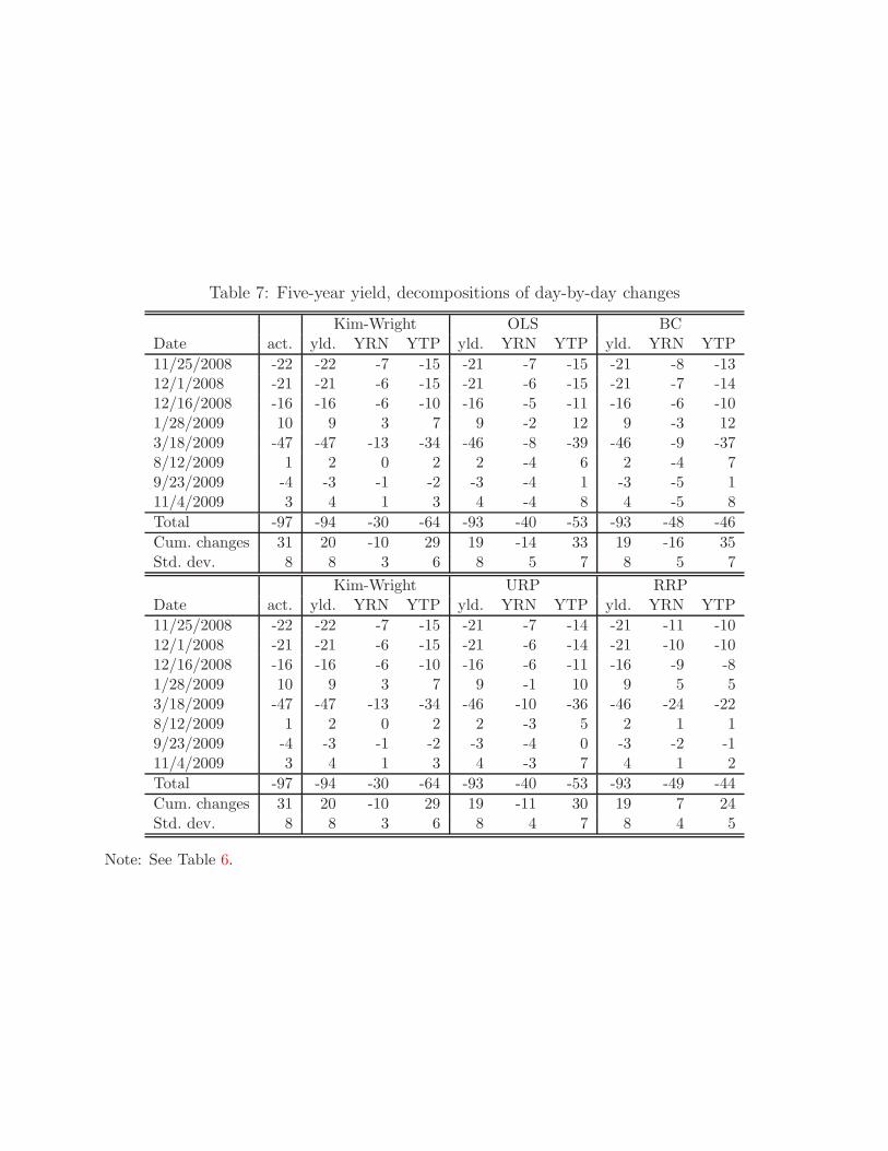
Table 7: Five-year yield, decompositions of day-by-day changes

Kim-Wright OLS BCDate act. yld. YRN YTP yld. YRN YTP yld. YRN YTP

11/25/2008 -22 -22 -7 -15 -21 -7 -15 -21 -8 -1312/1/2008 -21 -21 -6 -15 -21 -6 -15 -21 -7 -1412/16/2008 -16 -16 -6 -10 -16 -5 -11 -16 -6 -101/28/2009 10 9 3 7 9 -2 12 9 -3 123/18/2009 -47 -47 -13 -34 -46 -8 -39 -46 -9 -378/12/2009 1 2 0 2 2 -4 6 2 -4 79/23/2009 -4 -3 -1 -2 -3 -4 1 -3 -5 111/4/2009 3 4 1 3 4 -4 8 4 -5 8

Total -97 -94 -30 -64 -93 -40 -53 -93 -48 -46

Cum. changes 31 20 -10 29 19 -14 33 19 -16 35Std. dev. 8 8 3 6 8 5 7 8 5 7

Kim-Wright URP RRPDate act. yld. YRN YTP yld. YRN YTP yld. YRN YTP

11/25/2008 -22 -22 -7 -15 -21 -7 -14 -21 -11 -1012/1/2008 -21 -21 -6 -15 -21 -6 -14 -21 -10 -1012/16/2008 -16 -16 -6 -10 -16 -6 -11 -16 -9 -81/28/2009 10 9 3 7 9 -1 10 9 5 53/18/2009 -47 -47 -13 -34 -46 -10 -36 -46 -24 -228/12/2009 1 2 0 2 2 -3 5 2 1 19/23/2009 -4 -3 -1 -2 -3 -4 0 -3 -2 -111/4/2009 3 4 1 3 4 -3 7 4 1 2

Total -97 -94 -30 -64 -93 -40 -53 -93 -49 -44

Cum. changes 31 20 -10 29 19 -11 30 19 7 24Std. dev. 8 8 3 6 8 4 7 8 4 5

Note: See Table 6.

Figure 1: Shifts of futures-implied policy paths around key LSAP dates

0 5 10 15 20 25 30 35

0.0

0.5

1.0

1.5

2.0

perc

ent

beforeafter

25 November 2008

0 5 10 15 20 25 30 35

0.0

0.5

1.0

1.5

2.0

1 December 2008

0 5 10 15 20 25 30 35

0.0

0.5

1.0

1.5

2.0

perc

ent

16 December 2008

0 5 10 15 20 25 30 35

0.0

0.5

1.0

1.5

2.0

months forward

28 January 2009

0 5 10 15 20 25 30 35

0.0

0.5

1.0

1.5

2.0

months forward

perc

ent

18 March 2009

Note: Policy paths before and after five key LSAP announcements that are implied by marketrates of federal funds futures and Eurodollar futures. For details on calculation, refer to main text.

Figure 2: Shift of forward curve and policy path: OLS vs. BC

0 20 40 60 80 120

−15

0−

100

−50

0

months forward

basi

s po

ints

OLS

forward ratesexpectationsconf. int.

0 20 40 60 80 120

−15

0−

100

−50

0

months forward

Bias−corrected (BC)

Note: Cumulative changes, in basis points, on announcement days in fitted forward rates (solidline) and policy expectations (dashed line) together with 95%-confidence intervals for changes inexpectations (dotted lines). Left panel shows decomposition based on OLS estimates, right panelfor BC estimates.

Figure 3: Shift of forward curve and policy path: URP vs. RRP

0 20 40 60 80 120

−10

0−

500

months forward

basi

s po

ints

Unrestr. risk prices (URP)

forward ratesexpectationsconf. int.

0 20 40 60 80 120

−10

0−

500

months forward

Restr. risk prices (RRP)

Note: Cumulative changes, in basis points, on announcement days in fitted forward rates (solidline) and policy expectations (dashed line) together with 95%-confidence intervals for changes inexpectations (dotted lines). Left panel shows decomposition based on URP estimates, right panelfor RRP estimates.