The Short-Run Effects of a Natural Disaster With Imperfect Interregional Labour Mobility An Illustrative Application of a Prototype Multi-Regional CGE Model of the New Zealand Economy Nathaniel Robson 1 Abstract A multi-regional computable general equilibrium (CGE) model is used to sim- ulate the short-run economic impact of a natural disaster that strikes the central business district of Wellington, the capital city of New Zealand. A key feature of the analysis is the inclusion of an endogenous interregional mi- gration response to the loss of regional amenities — interpreted broadly as regional characteristics that enhance utility over and above that derived from consumption of market goods — along with feedbacks from regional real wage relativities. The model economy describes the behaviour of twenty-five indus- tries across five regions built upon bottom-up micro-foundations. As official, statistically estimated regional input-output tables are not produced in New Zealand, a maximum-entropy information-theoretic approach is used to derive the multi-regional input-output database required for model calibration. The natural disaster scenario assumes that capital of industries concentrated in the Wellington central business district is rendered inoperative at least tem- porarily but there are no fatalities. The time period considered is too short for insurance claims to be paid out on and the government response is limited to endogenous changes in the composition of its consumption expenditure. The analysis of the simulation results considers the role that regional char- acteristics and interdependencies play in generating the computed short-run outcomes. 1 The author has recently completed the requirements for a PhD degree in economics at Victoria University of Wellington, Wellington, New Zealand. The present paper extends upon research undertaken towards that qualification.

Welcome message from author
This document is posted to help you gain knowledge. Please leave a comment to let me know what you think about it! Share it to your friends and learn new things together.
Transcript

The Short-Run Effects of a Natural Disaster
With Imperfect Interregional Labour Mobility
An Illustrative Application of a Prototype
Multi-Regional CGE Model of the New Zealand Economy
Nathaniel Robson1
Abstract
A multi-regional computable general equilibrium (CGE) model is used to sim-
ulate the short-run economic impact of a natural disaster that strikes the
central business district of Wellington, the capital city of New Zealand. A
key feature of the analysis is the inclusion of an endogenous interregional mi-
gration response to the loss of regional amenities — interpreted broadly as
regional characteristics that enhance utility over and above that derived from
consumption of market goods — along with feedbacks from regional real wage
relativities. The model economy describes the behaviour of twenty-five indus-
tries across five regions built upon bottom-up micro-foundations. As official,
statistically estimated regional input-output tables are not produced in New
Zealand, a maximum-entropy information-theoretic approach is used to derive
the multi-regional input-output database required for model calibration. The
natural disaster scenario assumes that capital of industries concentrated in
the Wellington central business district is rendered inoperative at least tem-
porarily but there are no fatalities. The time period considered is too short
for insurance claims to be paid out on and the government response is limited
to endogenous changes in the composition of its consumption expenditure.
The analysis of the simulation results considers the role that regional char-
acteristics and interdependencies play in generating the computed short-run
outcomes.
1The author has recently completed the requirements for a PhD degree in economics at Victoria
University of Wellington, Wellington, New Zealand. The present paper extends upon research undertaken
towards that qualification.

CONTENTS 2
Contents
1 Introduction 3
2 The JENNIFER Model 4
3 Model Implementation 23
4 An Illustrative Application 36
5 Conclusion 52
Appendices 53
A List of Model Variables 54
B List of Model Equations 57
C Additional Results 69
References 81

1 INTRODUCTION 3
1 Introduction
On February 22, 2011 a magnitude 6.3 earthquake struck the city of Christchurch, New
Zealand’s second largest city. Land and buildings already weakened by a magnitude 7.1
quake six months earlier sustained extensive damage and some buildings in the central
business district collapsed with tragic consequences. In total, 185 lives were lost in the
earthquake. The economic cost of the disaster has also been very high — preliminary
estimates indicate that GDP growth for 2011 was 1.5 percentage points lower due to the
earthquake and the cost of rebuilding the city will be at least $NZ15 billion (around 10 %
of GDP).2 Canterbury, the region in which the city of Christchurch is located, experienced
a decline in usually-resident population of around 5000 (about 1% of the regional total)
in the year to June 2011.3 Christchurch itself saw a larger fall in population with some
residents shifting to other parts of Canterbury while there were also population outflows
to other (particularly urban) areas and abroad.
Wellington is New Zealand’s third largest city and the country’s capital, with an
urban land area slightly smaller but a population slightly larger than Christchurch. With
a major fault line running through the centre of the central business district (CBD) and
hundreds of other minor faults in the urban area, the Wellington region is well-known for
its seismic activity. However, the last major quake to do serious damage to the CBD was
the magnitude 8.2 earthquake of 1855.4 In the wake of the Christchurch earthquake, it
is pertinent to consider the economic impact of a similar disaster occurring in Wellington
in the present day. One may wish to consider, for example, how the impact would be
different to that observed in Christchurch due to different regional characteristics and how
the public sector could respond to the disaster.
An applied tool that would be useful in investigating these kinds of issues is a multi-
regional CGE model of the New Zealand economy. A prototype model of this type has
2New Zealand Treasury estimates as reported in http://www.nzherald.co.nz/business/news/
article.cfm?c_id=3&objectid=10710515, accessed on September 1, 2012.3Statistics New Zealand estimates from http://www.stats.govt.nz/browse_for_stats/
population/estimates_and_projections/SubnationalPopulationEstimates_HOTPJun11/
Commentary.aspx, accessed on September 1, 2012.4See the entry in The Encyclopedia of New Zealand at http://www.teara.govt.nz/en/
historic-earthquakes/3 for details.

2 THE JENNIFER MODEL 4
recently been developed as part of PhD research at Victoria University of Wellington,
New Zealand. The model, known as JENNIFER, is documented in the ensuing PhD
thesis, Robson (2012). This paper presents results from the application of the JENNIFER
model to a natural disaster scenario whereby some of the Wellington CBD capital stock is
rendered inoperative at least temporarily. As seen in the case of Christchurch, migration
may occur in the aftermath of the disaster. The concept of regional amenity is useful in
explaining these migration outflows: if regions have characteristics that enhance utility
over and above that derived from consumption of market goods, and households are able
to shift between regions, a deterioration of the utility-enhancing characteristics of a region
will lead to a net migration outflow. On the other hand, these migration outflows (and
the initial shock) will affect real wage relativities between regions, inducing a separate
migration response. The simulation results presented in this paper therefore consider the
impact not only of the damage to infrastructure, but also of migration flows resulting
from the loss of regional amenities and changes in real wage relativities.
A summary of the JENNIFER model is given in section 2. The third subsection
therein describes the procedure for simulating migration responses to changes in relative
amenities and real wage rates. Section 3 outlines how the model is implemented — the
key steps being database generation, calibration and closure. The simulation results of
the short-run natural disaster scenario are presented and discussed in section 4 before
concluding remarks in section 5.
2 The JENNIFER Model
The theoretical structure of the JENNIFER model is similar to that of other well-known
comparative-static CGE models in that it consists primarily of demand functions derived
from constrained optimisation and competitive equilibrium conditions. A key distinc-
tive feature of the model is that bottom-up microfoundations are used for the regional
modelling. That is, the aggregate economy is described as the sum of a set of interdepen-
dent regional economies. Households, firms, and endowments are assigned to regions and
agents face region-specific prices. Fundamental to this is the extension of the Armington
assumption — that domestic and imported varieties of otherwise identical products are

2 THE JENNIFER MODEL 5
not perfect substitutes — to products from different regions within the domestic economy.
Extensions to the model core allow for distribution services to be used in the delivery of
products from sellers to buyers, and households to respond to changes in regional ameni-
ties and wage relativities by shifting between regions.
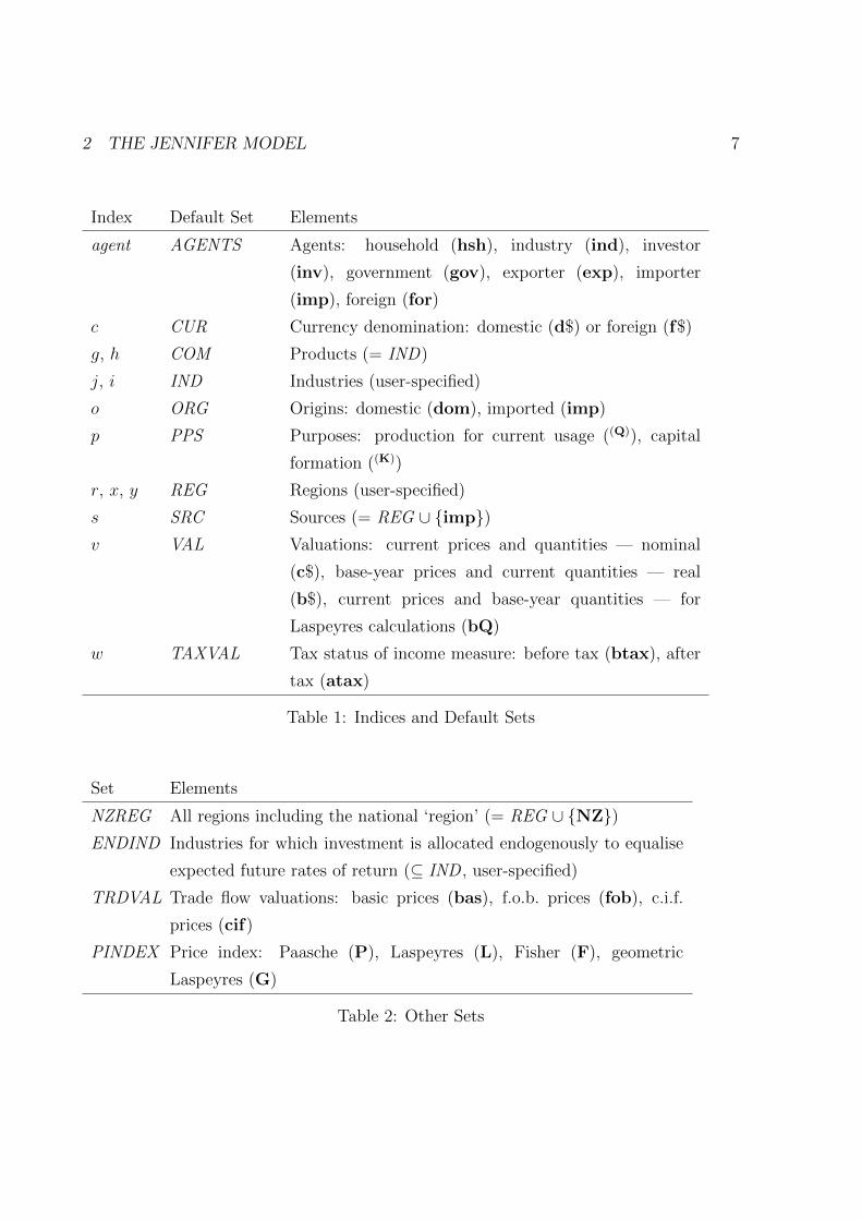
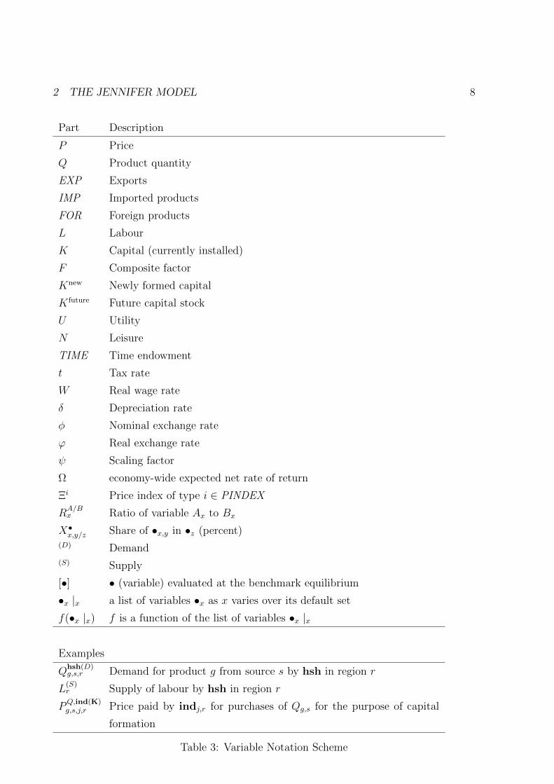
This section summarises the model structure. Due to its complexity, a scheme of
notation is adopted for expressing the model relationships in mathematical form. Multiple
index superscripts and subscripts are used in variable symbols to allow the model to be
written compactly. Table 1 lists the indices used and the corresponding set over which
they can be assumed to vary unless otherwise specified. Table 2 lists some other, less
commonly used sets of the model. Components used in variable symbols are set out in
table 3. The formation of parameter symbols follows analogously.
All economic activity is modelled as undertaken by representative agents, whether
those agents are optimising or are following some fixed behaviour rule. This implies an
assumption that the decisions made by all the people, firms, or organisations an agent
represents can be combined as though they make decisions as a single entity. That is,
they can be aggregated up to act as a single regional or national agent. In this model,
there are seven types of agent:
Households: one agent per region, representing the regional population. These agents
consume products and leisure, save, and supply labour to local industries. They are
also assumed to ultimately own the capital stock located in their region.
Industries: one agent per region for each industry. These agents demand inputs for
both current production and capital formation, although factors are only used for
the first of these. For simplicity it is assumed that each industry produces a single
unique product type.
Investor: one agent representing all industries collectively, who allocates the national
investment budget across industries and regions.
Government: one agent who decides the pattern of government consumption and tax-
ation
2 THE JENNIFER MODEL 6
Exporters: one agent per product type (i.e. per industry) who purchases domestic prod-
ucts and sells them to the foreign agent.
Importers: one agent per product type (i.e. per industry) who purchases foreign prod-
ucts and sells them to domestic agents.
Foreign: one agent who demands exports from and supplies foreign products to the
domestic economy.
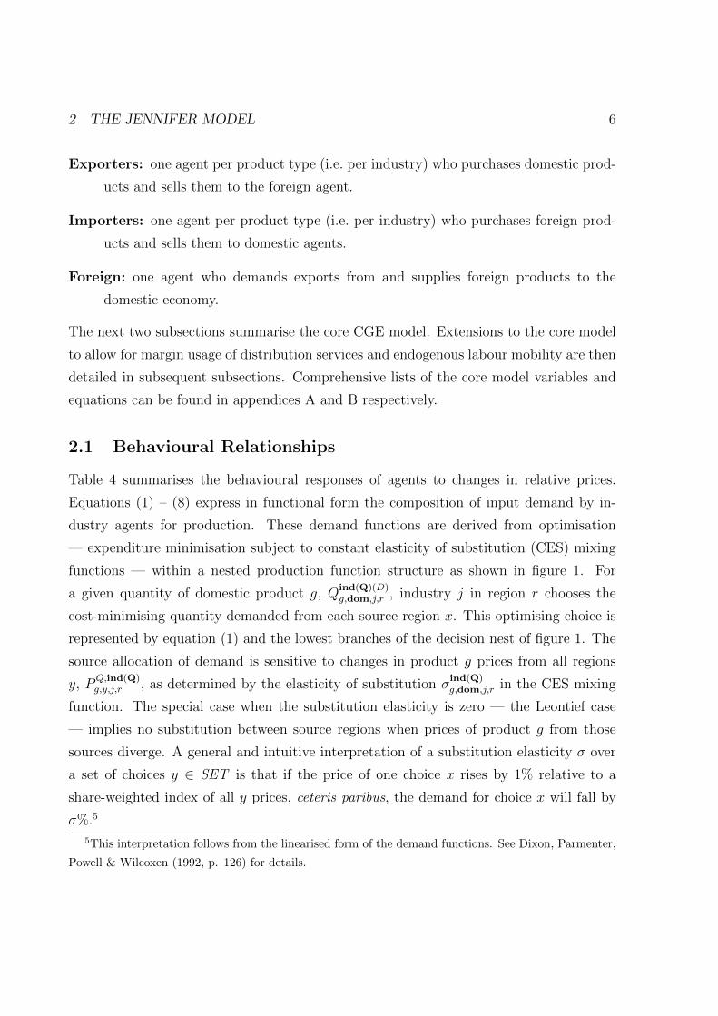
The next two subsections summarise the core CGE model. Extensions to the core model
to allow for margin usage of distribution services and endogenous labour mobility are then
detailed in subsequent subsections. Comprehensive lists of the core model variables and
equations can be found in appendices A and B respectively.
2.1 Behavioural Relationships
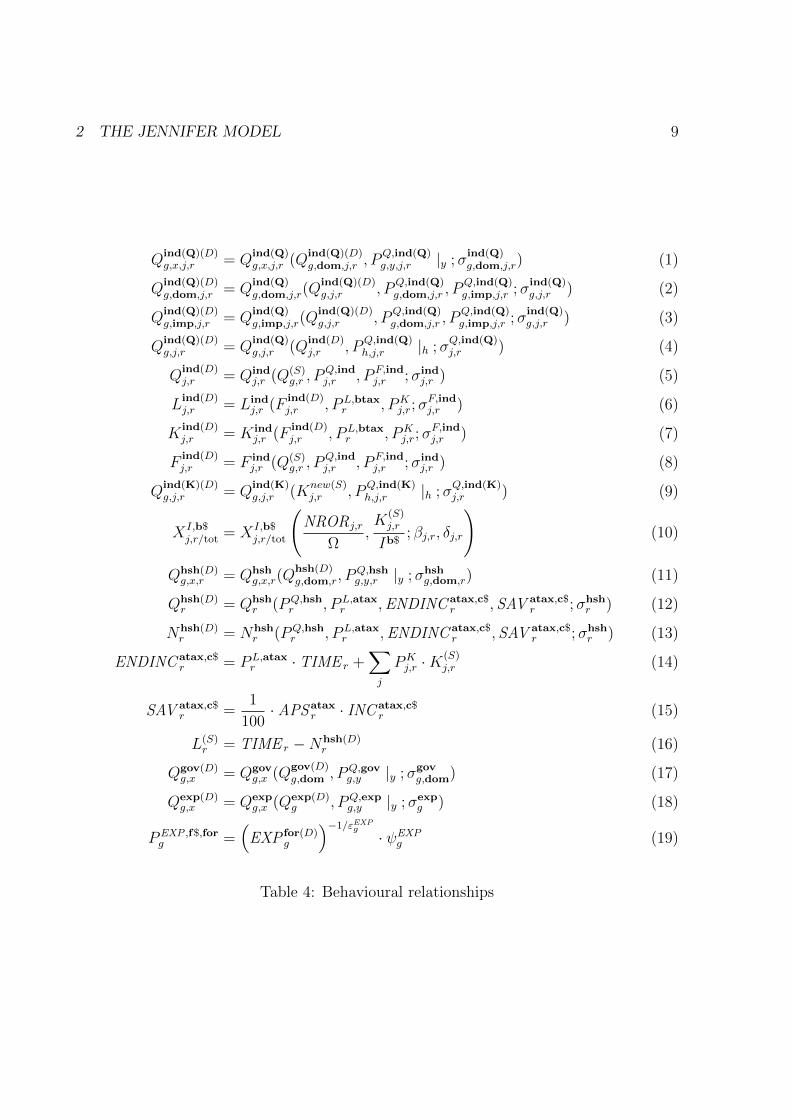
Table 4 summarises the behavioural responses of agents to changes in relative prices.
Equations (1) – (8) express in functional form the composition of input demand by in-
dustry agents for production. These demand functions are derived from optimisation
— expenditure minimisation subject to constant elasticity of substitution (CES) mixing
functions — within a nested production function structure as shown in figure 1. For
a given quantity of domestic product g, Qind(Q)(D)g,dom,j,r , industry j in region r chooses the
cost-minimising quantity demanded from each source region x. This optimising choice is
represented by equation (1) and the lowest branches of the decision nest of figure 1. The
source allocation of demand is sensitive to changes in product g prices from all regions
y, PQ,ind(Q)g,y,j,r , as determined by the elasticity of substitution σ
ind(Q)g,dom,j,r in the CES mixing
function. The special case when the substitution elasticity is zero — the Leontief case
— implies no substitution between source regions when prices of product g from those
sources diverge. A general and intuitive interpretation of a substitution elasticity σ over
a set of choices y ∈ SET is that if the price of one choice x rises by 1% relative to a
share-weighted index of all y prices, ceteris paribus, the demand for choice x will fall by
σ%.5
5This interpretation follows from the linearised form of the demand functions. See Dixon, Parmenter,
Powell & Wilcoxen (1992, p. 126) for details.
2 THE JENNIFER MODEL 7
Index Default Set Elements
agent AGENTS Agents: household (hsh), industry (ind), investor
(inv), government (gov), exporter (exp), importer
(imp), foreign (for)
c CUR Currency denomination: domestic (d$) or foreign (f$)
g, h COM Products (= IND)
j, i IND Industries (user-specified)
o ORG Origins: domestic (dom), imported (imp)
p PPS Purposes: production for current usage ((Q)), capital
formation ((K))
r, x, y REG Regions (user-specified)
s SRC Sources (= REG ∪ imp)v VAL Valuations: current prices and quantities — nominal
(c$), base-year prices and current quantities — real
(b$), current prices and base-year quantities — for
Laspeyres calculations (bQ)
w TAXVAL Tax status of income measure: before tax (btax), after
tax (atax)
Table 1: Indices and Default Sets
Set Elements
NZREG All regions including the national ‘region’ (= REG ∪ NZ)ENDIND Industries for which investment is allocated endogenously to equalise
expected future rates of return (⊆ IND , user-specified)
TRDVAL Trade flow valuations: basic prices (bas), f.o.b. prices (fob), c.i.f.
prices (cif)
PINDEX Price index: Paasche (P), Laspeyres (L), Fisher (F), geometric
Laspeyres (G)
Table 2: Other Sets
2 THE JENNIFER MODEL 8
Part Description
P Price
Q Product quantity
EXP Exports
IMP Imported products
FOR Foreign products
L Labour
K Capital (currently installed)
F Composite factor
Knew Newly formed capital
K future Future capital stock
U Utility
N Leisure
TIME Time endowment
t Tax rate
W Real wage rate
δ Depreciation rate
φ Nominal exchange rate
ϕ Real exchange rate
ψ Scaling factor
Ω economy-wide expected net rate of return
Ξi Price index of type i ∈ PINDEX
RA/Bx Ratio of variable Ax to Bx
X•x,y/z Share of •x,y in •z (percent)(D) Demand(S) Supply
[•] • (variable) evaluated at the benchmark equilibrium
•x |x a list of variables •x as x varies over its default set
f(•x |x) f is a function of the list of variables •x |x
Examples
Qhsh(D)g,s,r Demand for product g from source s by hsh in region r
L(S)r Supply of labour by hsh in region r
PQ,ind(K)g,s,j,r Price paid by indj,r for purchases of Qg,s for the purpose of capital
formation
Table 3: Variable Notation Scheme
2 THE JENNIFER MODEL 9
Qind(Q)(D)g,x,j,r = Q
ind(Q)g,x,j,r (Q
ind(Q)(D)g,dom,j,r , P
Q,ind(Q)g,y,j,r |y ;σ
ind(Q)g,dom,j,r) (1)
Qind(Q)(D)g,dom,j,r = Q
ind(Q)g,dom,j,r(Q
ind(Q)(D)g,j,r , P
Q,ind(Q)g,dom,j,r , P
Q,ind(Q)g,imp,j,r ;σ
ind(Q)g,j,r ) (2)
Qind(Q)(D)g,imp,j,r = Q
ind(Q)g,imp,j,r(Q
ind(Q)(D)g,j,r , P
Q,ind(Q)g,dom,j,r , P
Q,ind(Q)g,imp,j,r ;σ
ind(Q)g,j,r ) (3)
Qind(Q)(D)g,j,r = Q
ind(Q)g,j,r (Q
ind(D)j,r , P
Q,ind(Q)h,j,r |h ;σ
Q,ind(Q)j,r ) (4)
Qind(D)j,r = Qind
j,r (Q(S)g,r , P
Q,indj,r , P F,ind
j,r ;σindj,r ) (5)
Lind(D)j,r = Lind
j,r (Find(D)j,r , PL,btax
r , PKj,r;σ
F,indj,r ) (6)
Kind(D)j,r = K ind
j,r (Find(D)j,r , PL,btax
r , PKj,r;σ
F,indj,r ) (7)
Find(D)j,r = F ind
j,r (Q(S)g,r , P
Q,indj,r , P F,ind
j,r ;σindj,r ) (8)
Qind(K)(D)g,j,r = Q
ind(K)g,j,r (K
new(S)j,r , P
Q,ind(K)h,j,r |h ;σ
Q,ind(K)j,r ) (9)
XI,b$j,r/tot = XI,b$
j,r/tot
(NRORj,r
Ω,K
(S)j,r
Ib$; βj,r, δj,r
)(10)
Qhsh(D)g,x,r = Qhsh
g,x,r(Qhsh(D)g,dom,r, P
Q,hshg,y,r |y ;σhsh
g,dom,r) (11)
Qhsh(D)r = Qhsh
r (PQ,hshr , PL,atax
r ,ENDINC atax,c$r , SAV atax,c$
r ;σhshr ) (12)
Nhsh(D)r = Nhsh
r (PQ,hshr , PL,atax
r ,ENDINC atax,c$r , SAV atax,c$
r ;σhshr ) (13)
ENDINC atax,c$r = PL,atax
r · TIME r +∑j
PKj,r ·K
(S)j,r (14)
SAV atax,c$r =
1
100· APS atax
r · INC atax,c$r (15)
L(S)r = TIME r −Nhsh(D)
r (16)
Qgov(D)g,x = Qgov
g,x (Qgov(D)g,dom , PQ,gov
g,y |y ;σgovg,dom) (17)
Qexp(D)g,x = Qexp
g,x (Qexp(D)g , PQ,exp
g,y |y ;σexpg ) (18)
PEXP ,f$,forg =
(EXP for(D)
g
)−1/εEXPg
· ψEXPg (19)
Table 4: Behavioural relationships
Output
Materials / Factors
Product g 1,2,…
Origin o dom,imp
Source region x A,B,…
ind,
,
Q
rj
ind
rgQ
,
ind
rj ,
ind
rjQ
,
ind
rjF
,
ind,
,
F
rj
ind
rjL
,
ind
rjK
, Labour / Capital
ind
1 rjQ
,,
ind
2 rjQ
,,
ind
dom2 rj ,,,
ind
A2 rjQ
,,,
ind
B2 rjQ
,,,
ind
1 rj ,,
ind
dom1 rjQ
,,,
ind
imp1 rjQ
,,,
ind
2 rj ,,
ind
dom2 rjQ
,,,
ind
imp2 rjQ
,,,
ind
A1 rjQ
,,,
ind
B1 rjQ
,,,
ind
dom1 rj ,,,
2 THE JENNIFER MODEL 10
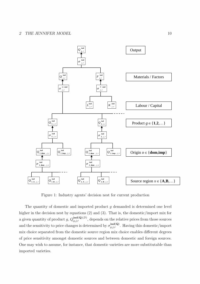
Figure 1: Industry agents’ decision nest for current production
The quantity of domestic and imported product g demanded is determined one level
higher in the decision nest by equations (2) and (3). That is, the domestic/import mix for
a given quantity of product g, Qind(Q)(D)g,j,r , depends on the relative prices from those sources
and the sensitivity to price changes is determined by σind(Q)g,j,r . Having this domestic/import
mix choice separated from the domestic source region mix choice enables different degrees
of price sensitivity amongst domestic sources and between domestic and foreign sources.
One may wish to assume, for instance, that domestic varieties are more substitutable than
imported varieties.
2 THE JENNIFER MODEL 11
The remainder of the decision nest for each industry j in each region r is described
analogously by the demand equations. The product mix of the agent’s intermediate input
Qind(D)j,r is given by the demand equations (4) which determine Q
ind(Q)(D)g,j,r for all products
g. The quantity of composite intermediate input demanded is in turn derived from cost
minimisation subject to a CES production function for Q(S)g,r (where g = j) using Q
ind(D)j,r
and composite factor Find(D)j,r as inputs. As shown in the decision nest and equations (6)
– (7), the composite factor input is a cost-minimising mix of labour Lind(D)j,r and capital
Kind(D)j,r .
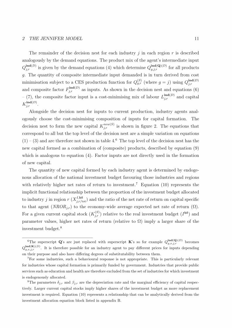
Alongside the decision nest for inputs to current production, industry agents anal-
ogously choose the cost-minimising composition of inputs for capital formation. The
decision nest to form the new capital Knew(S)j,r is shown in figure 2. The equations that
correspond to all but the top level of the decision nest are a simple variation on equations
(1) – (3) and are therefore not shown in table 4.6 The top level of the decision nest has the
new capital formed as a combination of (composite) products, described by equation (9)
which is analogous to equation (4). Factor inputs are not directly used in the formation
of new capital.
The quantity of new capital formed by each industry agent is determined by endoge-
nous allocation of the national investment budget favouring those industries and regions
with relatively higher net rates of return to investment.7 Equation (10) represents the
implicit functional relationship between the proportion of the investment budget allocated
to industry j in region r (XI,b$j,r/tot) and the ratio of the net rate of return on capital specific
to that agent (NRORj,r) to the economy-wide average expected net rate of return (Ω).
For a given current capital stock (K(S)j,r ) relative to the real investment budget (Ib$) and
parameter values, higher net rates of return (relative to Ω) imply a larger share of the
investment budget.8
6The superscript Q’s are just replaced with superscript K’s so for example Qind(Q)(D)g,x,j,r becomes
Qind(K)(D)g,x,j,r . It is therefore possible for an industry agent to pay different prices for inputs depending
on their purpose and also have differing degrees of substitutability between them.7For some industries, such a behavioural response is not appropriate. This is particularly relevant
for industries whose capital formation is primarily funded by government. Industries that provide public
services such as education and health are therefore excluded from the set of industries for which investment
is endogenously allocated.8The parameters δj,r and βj,r are the depreciation rate and the marginal efficiency of capital respec-
tively. Larger current capital stocks imply higher shares of the investment budget as more replacement
investment is required. Equation (10) represents a relationship that can be analytically derived from the
investment allocation equation block listed in appendix B.
New capital
Product g 1,2,…
Origin o dom,imp
Source region x A,B,…
ind,
,
Q
rj
new
rjK
,
ind
1 rjQ
,,
ind
2 rjQ
,,
ind
dom2 rj ,,,
ind
A2 rjQ
,,,
ind
B2 rjQ
,,,
ind
1 rj ,,
ind
dom1 rjQ
,,,
ind
imp1 rjQ
,,,
ind
2 rj ,,
ind
dom2 rjQ
,,,
ind
imp2 rjQ
,,,
ind
A1 rjQ
,,,
ind
B1 rjQ
,,,
ind
dom1 rj ,,,
2 THE JENNIFER MODEL 12
Figure 2: Industry agents’ decision nest for capital formation
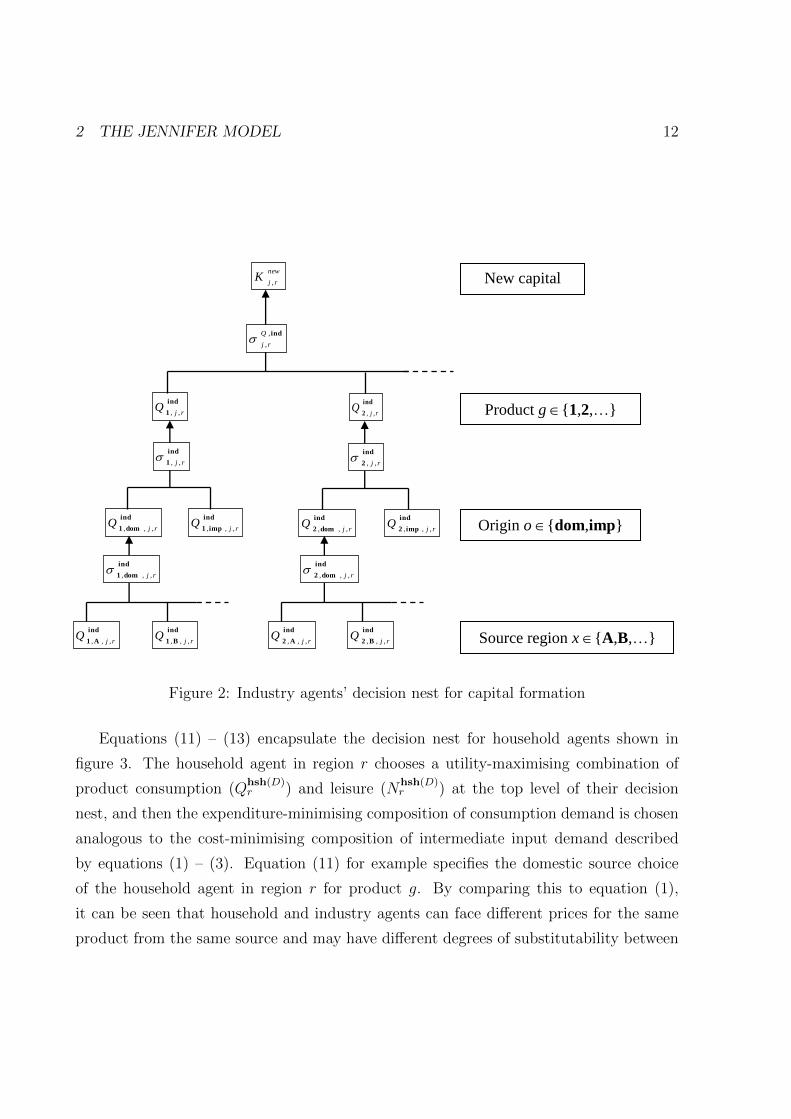
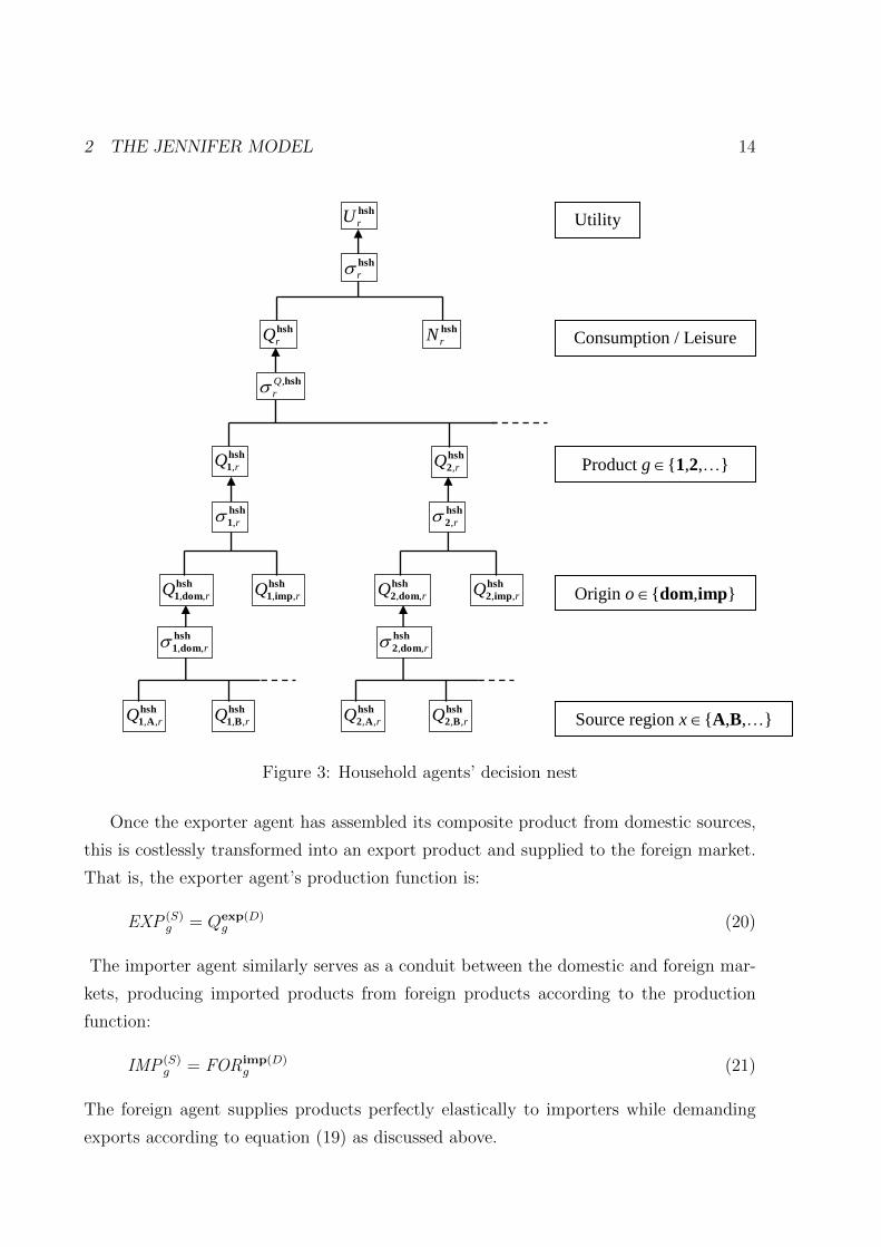
Equations (11) – (13) encapsulate the decision nest for household agents shown in
figure 3. The household agent in region r chooses a utility-maximising combination of
product consumption (Qhsh(D)r ) and leisure (N
hsh(D)r ) at the top level of their decision
nest, and then the expenditure-minimising composition of consumption demand is chosen
analogous to the cost-minimising composition of intermediate input demand described
by equations (1) – (3). Equation (11) for example specifies the domestic source choice
of the household agent in region r for product g. By comparing this to equation (1),
it can be seen that household and industry agents can face different prices for the same
product from the same source and may have different degrees of substitutability between
2 THE JENNIFER MODEL 13
sources. The utility-maximising choice at the top of the decision nest is made subject
to the constraint that the sum of consumption and leisure valued at current prices does
not exceed endowment income, defined in equation (14), net of saving, defined in equa-
tion (15). Endowment income is the sum of the time endowment (TIME r) valued at
the after-tax nominal wage rate (PL,ataxr ) and rental income from capital. The average
propensity to save (APS ataxr ) is exogenously specified such that equation (15) determines
household saving in region r as that proportion of household income (the sum of labour
and capital income). The household consumption / leisure choice leads via equation (16)
to an endogenous labour supply response to changes in the regional wage rate relative
to the price of consumption goods (i.e. the real wage rate). The time endowment is a
quantity proportional to the regional working age population so changes in labour supply
are reflected in changes in the labour force participation rate.
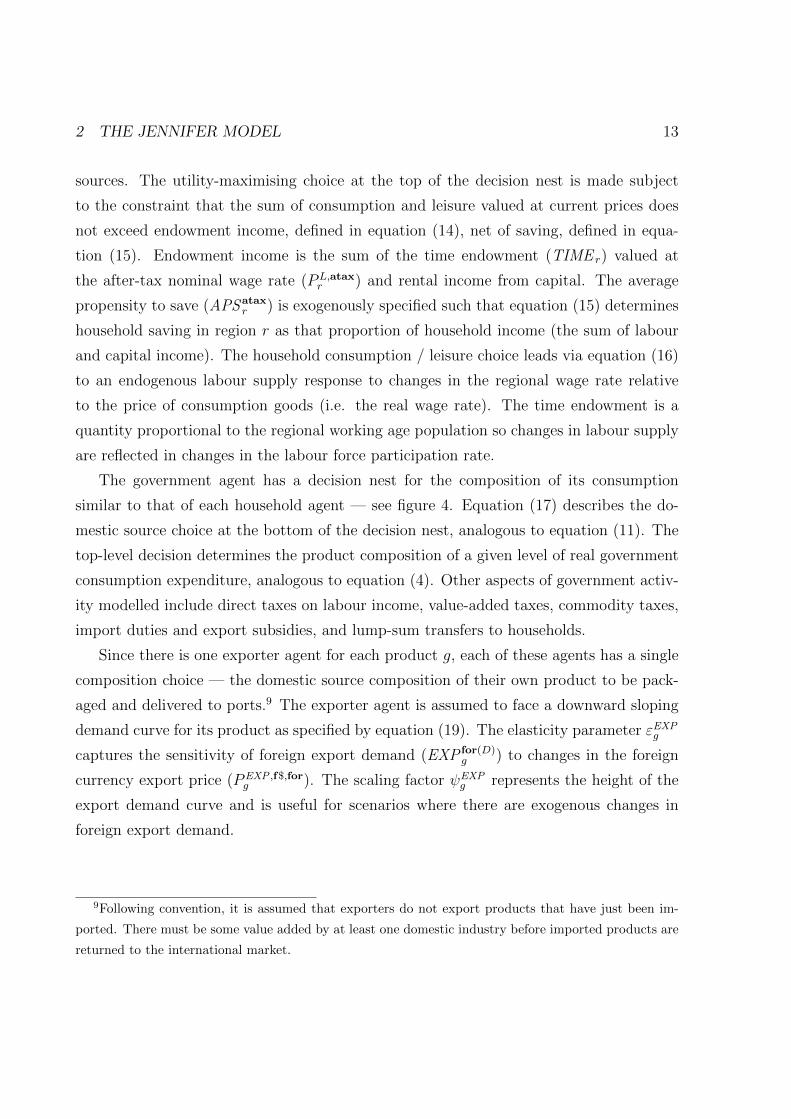
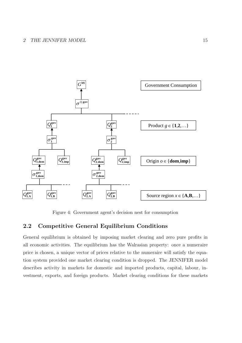
The government agent has a decision nest for the composition of its consumption
similar to that of each household agent — see figure 4. Equation (17) describes the do-
mestic source choice at the bottom of the decision nest, analogous to equation (11). The
top-level decision determines the product composition of a given level of real government
consumption expenditure, analogous to equation (4). Other aspects of government activ-
ity modelled include direct taxes on labour income, value-added taxes, commodity taxes,
import duties and export subsidies, and lump-sum transfers to households.
Since there is one exporter agent for each product g, each of these agents has a single
composition choice — the domestic source composition of their own product to be pack-
aged and delivered to ports.9 The exporter agent is assumed to face a downward sloping
demand curve for its product as specified by equation (19). The elasticity parameter εEXPg
captures the sensitivity of foreign export demand (EXP for(D)g ) to changes in the foreign
currency export price (PEXP ,f$,forg ). The scaling factor ψEXP
g represents the height of the
export demand curve and is useful for scenarios where there are exogenous changes in
foreign export demand.
9Following convention, it is assumed that exporters do not export products that have just been im-
ported. There must be some value added by at least one domestic industry before imported products are
returned to the international market.
Utility
Consumption / Leisure
Product g 1,2,…
Origin o dom,imp
Source region x A,B,…
hsh
dom2 r,,
hsh
A2 rQ ,,
hsh
B2 rQ ,,
hsh
A1 rQ ,,
hsh
B1 rQ ,,
hsh
dom1 r,,
hsh
1 r,
hsh
dom1 rQ ,,
hsh
imp1 rQ ,,
hsh
2 r,
hsh
dom2 rQ ,,
hsh
imp2 rQ ,,
hsh,Q
r
hsh
1 rQ ,
hsh
2 rQ ,
hsh
rU
hsh
r
hsh
rQ hsh
rN
2 THE JENNIFER MODEL 14
Figure 3: Household agents’ decision nest
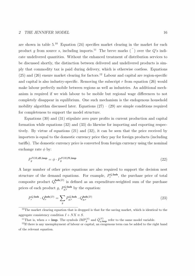
Once the exporter agent has assembled its composite product from domestic sources,
this is costlessly transformed into an export product and supplied to the foreign market.
That is, the exporter agent’s production function is:
EXP (S)g = Qexp(D)
g (20)
The importer agent similarly serves as a conduit between the domestic and foreign mar-
kets, producing imported products from foreign products according to the production
function:
IMP (S)g = FORimp(D)
g (21)
The foreign agent supplies products perfectly elastically to importers while demanding
exports according to equation (19) as discussed above.
Government Consumption
Product g 1,2,…
Origin o dom,imp
Source region x A,B,…
gov,Q
b$G
gov
1Q
gov
dom2,
gov
A2,Q gov
B2,Q
gov
1
gov
dom1,Q gov
imp1,Q
gov
2
gov
dom2,Q gov
imp2,Q
gov
A1,Q gov
B1,Q
gov
dom1,
gov
2Q
2 THE JENNIFER MODEL 15
Figure 4: Government agent’s decision nest for consumption
2.2 Competitive General Equilibrium Conditions
General equilibrium is obtained by imposing market clearing and zero pure profits in
all economic activities. The equilibrium has the Walrasian property: once a numeraire
price is chosen, a unique vector of prices relative to the numeraire will satisfy the equa-
tion system provided one market clearing condition is dropped. The JENNIFER model
describes activity in markets for domestic and imported products, capital, labour, in-
vestment, exports, and foreign products. Market clearing conditions for these markets
2 THE JENNIFER MODEL 16
are shown in table 5.10 Equation (24) specifies market clearing in the market for each
product g from source s, including imports.11 The breve marks ( ˘ ) over the Q’s indi-
cate undelivered quantities. Without the enhanced treatment of distribution services to
be discussed shortly, the distinction between delivered and undelivered products is sim-
ply that commodity tax is paid during delivery, which is otherwise costless. Equations
(25) and (26) ensure market clearing for factors.12 Labour and capital are region-specific
and capital is also industry-specific. Removing the subscript r from equation (26) would
make labour perfectly mobile between regions as well as industries. An additional mech-
anism is required if we wish labour to be mobile but regional wage differences to not
completely disappear in equilibrium. One such mechanism is the endogenous household
mobility algorithm discussed later. Equations (27) – (29) are simple conditions required
for completeness to support the model structure.
Equations (30) and (31) stipulate zero pure profits in current production and capital
formation while equations (32) and (33) do likewise for importing and exporting respec-
tively. By virtue of equations (21) and (32), it can be seen that the price received by
importers is equal to the domestic currency price they pay for foreign products (including
tariffs). The domestic currency price is converted from foreign currency using the nominal
exchange rate φ by:
PFOR,d$,impg = φ · PFOR,f$,imp
g (22)
A large number of other price equations are also required to support the decision nest
structure of the demand equations. For example, PQ,hshr , the purchase price of total
composite product Qhsh(D)r is defined as an expenditure-weighted sum of the purchase
prices of each product g, PQ,hshg,r by the equation:
PQ,hshr ·Qhsh(D)
r =∑g
PQ,hshg,r ·Qhsh(D)
g,r (23)
10The market clearing equation that is dropped is that for the saving market, which is identical to the
aggregate consistency condition I +NX ≡ S.11That is, when s = imp. The symbols IMP (S)
g and Q(S)g,imp refer to the same model variable.
12If there is any unemployment of labour or capital, an exogenous term can be added to the right hand
of the relevant equation.

2 THE JENNIFER MODEL 17
Q(S)g,s =
∑r
Qhsh(D)g,s,r +
∑p
∑j
∑r
Qind(p)(D)g,s,j,r + Qgov(D)
g,s + Qexp(D)g,s (24)
K(S)j,r = K
ind(D)j,r (25)
L(S)r =
∑j
Lind(D)j,r (26)
Knew(S)j,r = I
ind(D)j,r (27)
EXP (S)g = EXP for(D)
g (28)
FOR(S)g = FORimp(D)
g (29)
PQg,r · Q(S)
g,r = PQ,indj,r ·Qind(D)
j,r + P F,indj,r · F ind(D)
j,r ∀g = j (30)
PK,newj,r ·Knew(S)
j,r =∑g
PQ,ind(K)g,j,r ·Qind(K)(D)
g,j,r (31)
P IMPg · IMP (S)
g = PFOR,d$,impg · FORimp(D)
g (32)
PEXPg · EXP (S)
g = PQ,expg ·Qexp(D)
g (33)
Table 5: Competitive general equilibrium conditions
All other purchase prices involved in the agents’ decision nests are similarly defined as
weighted averages of the prices one level down. The prices at the bottom of the decision
nests, such as PQ,hshg,s,r , are functions of the basic price received by the seller and all costs
involved in delivery, including taxes and margins. For this reason, these will be discussed
in the subsection on distribution services.
2.3 Other Equations
It is common practice and convenient here to assign the nominal exchange rate φ as the
numeraire for our simulations. The value of φ is fixed at an arbitrary level, essentially
making the nominal exchange rate exogenous to the model, by the equation:
φ = 1 (34)
Many other equations are included in the model to facilitate different closure assump-
tions and provide measures of economic activity for reporting. These equations typically
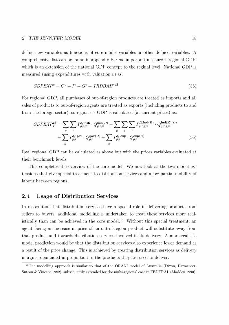
2 THE JENNIFER MODEL 18
define new variables as functions of core model variables or other defined variables. A
comprehensive list can be found in appendix B. One important measure is regional GDP,
which is an extension of the national GDP concept to the reginal level. National GDP is
measured (using expenditures with valuation v) as:
GDPEXPv = Cv + Iv +Gv + TRDBALv,d$ (35)
For regional GDP, all purchases of out-of-region products are treated as imports and all
sales of products to out-of-region agents are treated as exports (including products to and
from the foreign sector), so region r’s GDP is calculated (at current prices) as:
GDPEXPc$r =
∑g
∑x
PQ,hshg,r,x ·Qhsh(D)
g,r,x +∑g
∑j
∑x
PQ,ind(K)g,r,j,x ·Qind(K)(D)
g,r,j,x
+∑g
PQ,govg,r ·Qgov(D)
g,r +∑g
PQ,expg,r ·Qexp(D)
g,r (36)
Real regional GDP can be calculated as above but with the prices variables evaluated at
their benchmark levels.
This completes the overview of the core model. We now look at the two model ex-
tensions that give special treatment to distribution services and allow partial mobility of
labour between regions.
2.4 Usage of Distribution Services
In recognition that distribution services have a special role in delivering products from
sellers to buyers, additional modelling is undertaken to treat these services more real-
istically than can be achieved in the core model.13 Without this special treatment, an
agent facing an increase in price of an out-of-region product will substitute away from
that product and towards distribution services involved in its delivery. A more realistic
model prediction would be that the distribution services also experience lower demand as
a result of the price change. This is achieved by treating distribution services as delivery
margins, demanded in proportion to the products they are used to deliver.
13The modelling approach is similar to that of the ORANI model of Australia (Dixon, Parmenter,
Sutton & Vincent 1982), subsequently extended for the multi-regional case in FEDERAL (Madden 1990).

2 THE JENNIFER MODEL 19
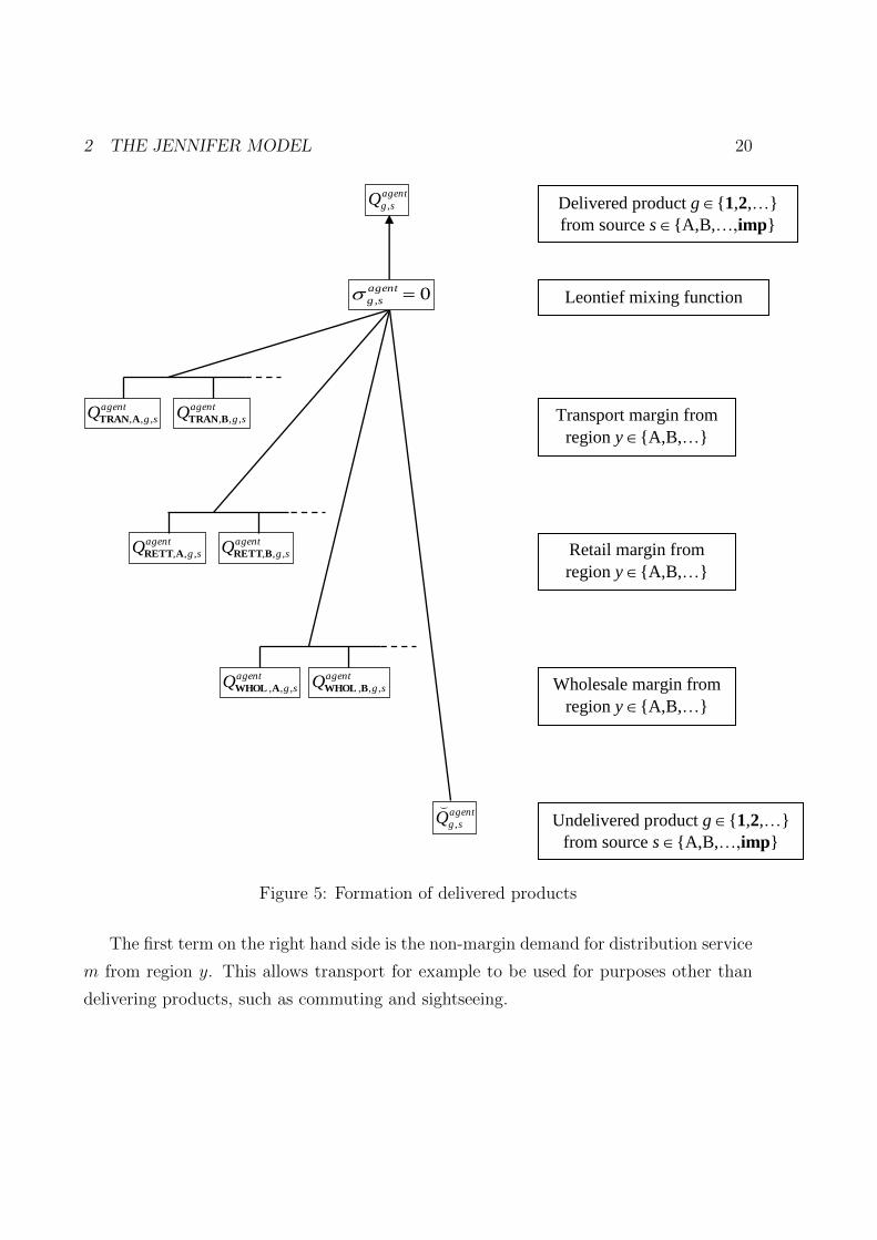
A distinction is made between delivered and undelivered products, where a delivered
product is viewed as a package of distribution services and the undelivered product. The
demands at the lowest levels of the decision nests in the core model are therefore demands
for these product packages rather than just the undelivered products. With the set of
distribution services MAR specified as consisting of wholesale trade (WHOL), retail trade
(RETT), and transportation (TRAN), the additional structure shown in figure 5 is added
to the lowest level of each agent’s decision nest (for each product from each source). In
terms of model equations, adding this structure is achieved by the inclusion of demand
functions for each agent of the form:
Qagent(D)g,s = aQ,agentg,s · Q
agent(D)g,s
vQ,agentg,s
(37)
Qagent(D)m,y,g,s = aQ,agentm,y,g,s ·
Qagent(D)g,s
vQ,agentg,s
(38)
These equations represent the solution to a given agent’s optimisation problem where
expenditure is minimised in obtaining the quantity Qagent(D)g,s of delivered product, which is
a Leontief combination of the undelivered product and the distribution services m ∈ MAR
(from regions y ∈ REG) used in its delivery. The a’s and v’s are parameters of the Leontief
function, evaluated during model calibration as discussed in section 3.
The price paid by purchasers can now be related to the price received by sellers, taxes
(including goods and services tax), and delivery costs by:
PQ,agentg,s ·Qagent(D)
g,s = PQg,s · (1 + tQ,agentg + tGST ,agent
g ) · Qagent(D)g,s
+∑m
∑y
PQm,y ·Qagent(D)
m,y,g,s (39)
The market clearing conditions for distribution services need to be altered to add in the
margin demands Qagent(D)m,y,g,s as follows:14
Q(S)m,y =
∑agent
(Q
agent(D)h,y · 1h=m +
∑g
∑s
Qagent(D)m,y,g,s
)(41)
141 is the indicator function:
1condition =
1 if condition = true
0 if condition = false(40)
Delivered product g 1,2,…
from source s A,B,…,imp
Leontief mixing function 0, agent
sg
agent
sgQ ,
agent
sgQ ,
agent
sgQ ,,,ARETT
agent
sgQ ,,,BRETT
agent
sgQ ,,,ATRAN
agent
sgQ ,,,BTRAN
agent
sgQ ,,,AWHOL
agent
sgQ ,,,BWHOL
Transport margin from
region y A,B,…
Retail margin from
region y A,B,…
Wholesale margin from
region y A,B,…
Undelivered product g 1,2,…
from source s A,B,…,imp
2 THE JENNIFER MODEL 20
Figure 5: Formation of delivered products
The first term on the right hand side is the non-margin demand for distribution service
m from region y. This allows transport for example to be used for purposes other than
delivering products, such as commuting and sightseeing.

2 THE JENNIFER MODEL 21
2.5 Partial Labour Mobility
Jones & Whalley (1989, page 375) argue that neither perfect labour mobility nor complete
labour immobility is an appropriate assumption when evaluating the regional impacts of
policy changes. They then proceed to set up an interesting micro-foundation for partial
labour mobility between regions. The approach allows migration flows to be endogenously
determined based on regional income differences.
The model extension that allows a similar labour mobility response in JENNIFER
is yet to have formally developed micro-foundations but goes further than the Jones &
Whalley (1989) modelling in two respects. Firstly, it recognises that changes in relative
regional amenity may also lead to migration flows. Secondly, feedbacks from the migration
flows to the regional economies are incorporated. There are two aspects to these feedbacks
that complicate obtaining a model solution in a single run: households are assumed
to respond to real wage rate relativities but real wage rates relativities depend on the
availability of labour across regions, and households are not assumed identical across
regions so migration affects the regional composition of households (in terms of working
age persons per household, non-labour force per household, etc.)
The general approach taken to obtain a model solution that takes into account house-
hold migration responses and feedbacks is to solve the model once for a given shock
(including changes in regional amenities), use the solution to calculate the mobility re-
sponse of households to the resulting real wage rate differences, and then solve the model
again with an updated shock that takes the mobility response into account.
Given solution values (in angle brackets 〈 〉) and benchmark equilibrium values (in
square brackets [ ]), the flows of households between regions due to changes in real wage
relativities are calculated by the formula:
HSH x→r
〈HSH x〉= max
θx,r100
(〈Wr〉〈Wx〉
− [Wr]
[Wx]
), 0
(42)
where HSH x→r is the flow of households from region x to region r
Wr is the pre-tax real wage rate in region r
θx,r is a parameter that represents the sensitivity of
households in region x to changes in the real wage rate
of region r relative to their own
2 THE JENNIFER MODEL 22
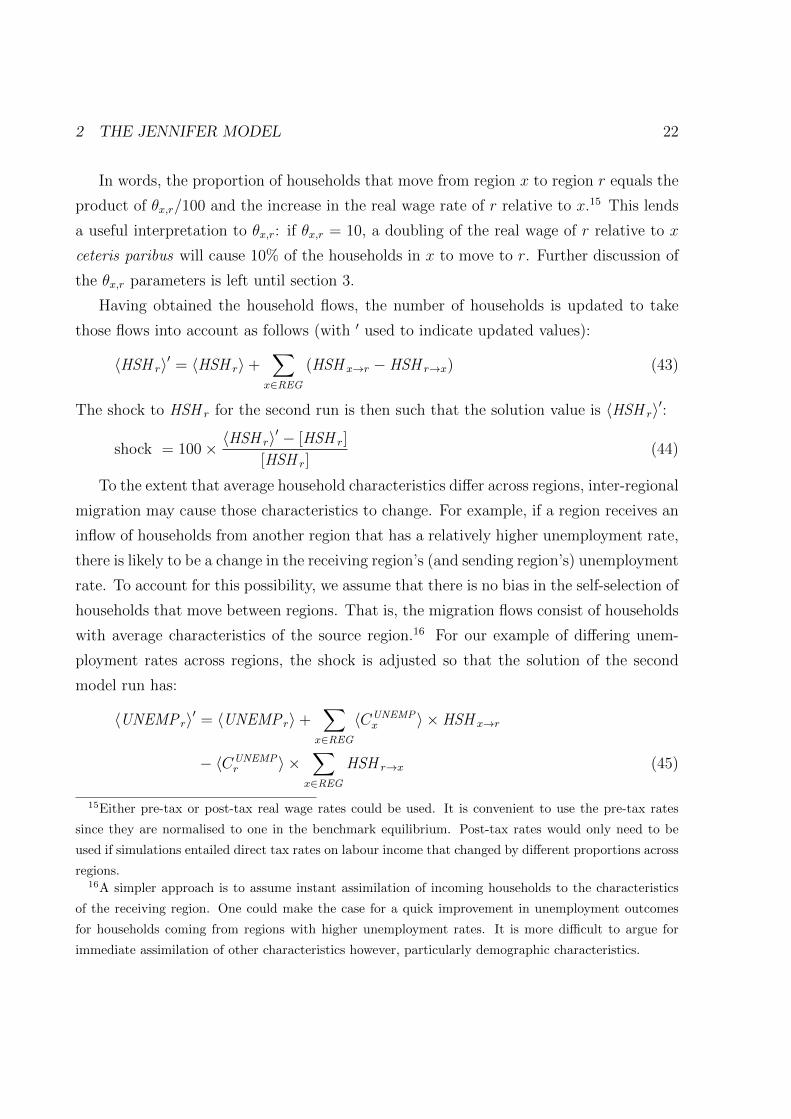
In words, the proportion of households that move from region x to region r equals the
product of θx,r/100 and the increase in the real wage rate of r relative to x.15 This lends
a useful interpretation to θx,r: if θx,r = 10, a doubling of the real wage of r relative to x
ceteris paribus will cause 10% of the households in x to move to r. Further discussion of
the θx,r parameters is left until section 3.
Having obtained the household flows, the number of households is updated to take
those flows into account as follows (with ′ used to indicate updated values):
〈HSH r〉′ = 〈HSH r〉+∑
x∈REG
(HSH x→r − HSH r→x) (43)
The shock to HSH r for the second run is then such that the solution value is 〈HSH r〉′:
shock = 100× 〈HSH r〉′ − [HSH r]
[HSH r](44)
To the extent that average household characteristics differ across regions, inter-regional
migration may cause those characteristics to change. For example, if a region receives an
inflow of households from another region that has a relatively higher unemployment rate,
there is likely to be a change in the receiving region’s (and sending region’s) unemployment
rate. To account for this possibility, we assume that there is no bias in the self-selection of
households that move between regions. That is, the migration flows consist of households
with average characteristics of the source region.16 For our example of differing unem-
ployment rates across regions, the shock is adjusted so that the solution of the second
model run has:
〈UNEMP r〉′ = 〈UNEMP r〉+∑
x∈REG
〈CUNEMPx 〉 × HSH x→r
− 〈CUNEMPr 〉 ×
∑x∈REG
HSH r→x (45)
15Either pre-tax or post-tax real wage rates could be used. It is convenient to use the pre-tax rates
since they are normalised to one in the benchmark equilibrium. Post-tax rates would only need to be
used if simulations entailed direct tax rates on labour income that changed by different proportions across
regions.16A simpler approach is to assume instant assimilation of incoming households to the characteristics
of the receiving region. One could make the case for a quick improvement in unemployment outcomes
for households coming from regions with higher unemployment rates. It is more difficult to argue for
immediate assimilation of other characteristics however, particularly demographic characteristics.
3 MODEL IMPLEMENTATION 23
where UNEMP r is the number of unemployed persons in region r
CUNEMPr is the average unemployed per household in region r
The inflow of unemployed from all other regions is added to unemployment in region r
and the outflow of unemployed is subtracted. Similar adjustments can be made to other
demographic and labour market measures as needed. The effect of these adjustments will
see some regions converge in average household characteristics but others to diverge.
With some minor adjustments, equation (42) and the updating formulae such as (43)
can include household flows to and from abroad in response to changes in regions’ real
wage rates relative to the foreign real wage.
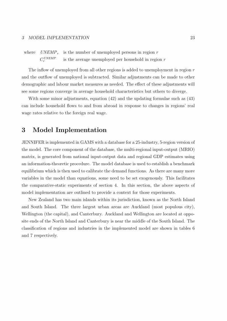
3 Model Implementation
JENNIFER is implemented in GAMS with a database for a 25-industry, 5-region version of
the model. The core component of the database, the multi-regional input-output (MRIO)
matrix, is generated from national input-output data and regional GDP estimates using
an information-theoretic procedure. The model database is used to establish a benchmark
equilibrium which is then used to calibrate the demand functions. As there are many more
variables in the model than equations, some need to be set exogenously. This facilitates
the comparative-static experiments of section 4. In this section, the above aspects of
model implementation are outlined to provide a context for those experiments.
New Zealand has two main islands within its jurisdiction, known as the North Island
and South Island. The three largest urban areas are Auckland (most populous city),
Wellington (the capital), and Canterbury. Auckland and Wellington are located at oppo-
site ends of the North Island and Canterbury is near the middle of the South Island. The
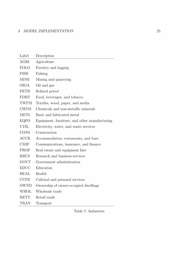
classification of regions and industries in the implemented model are shown in tables 6
and 7 respectively.
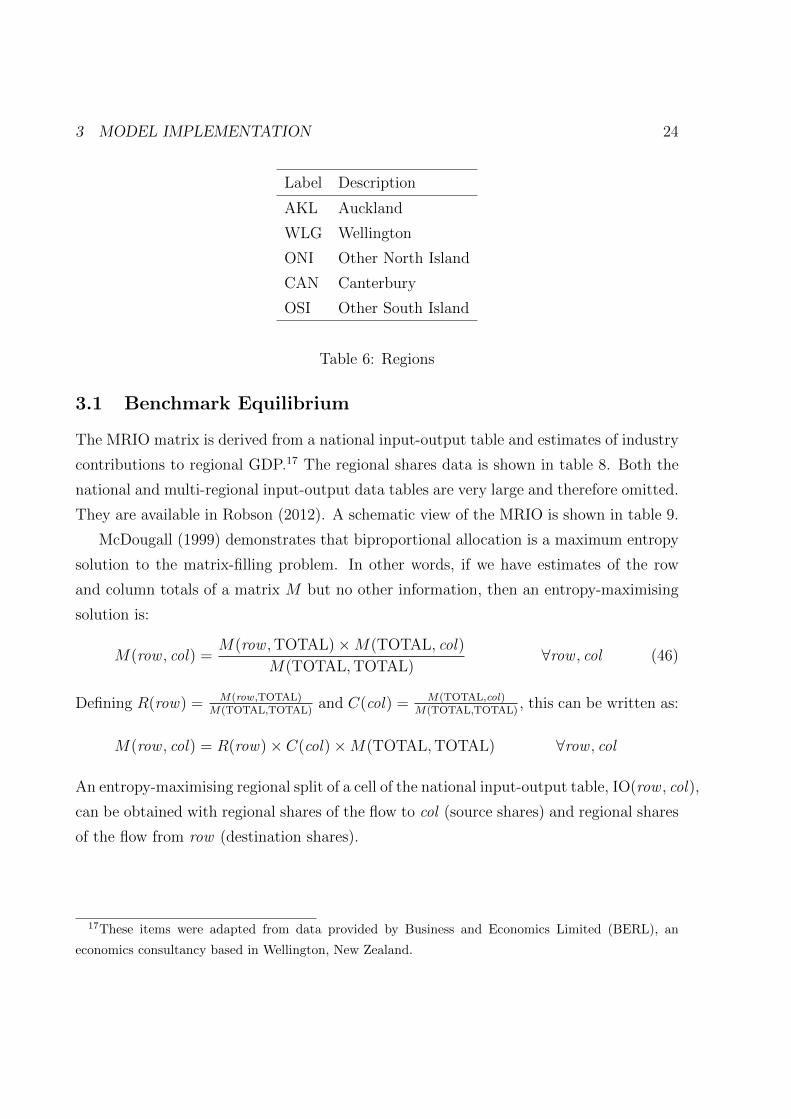
3 MODEL IMPLEMENTATION 24
Label Description
AKL Auckland
WLG Wellington
ONI Other North Island
CAN Canterbury
OSI Other South Island
Table 6: Regions
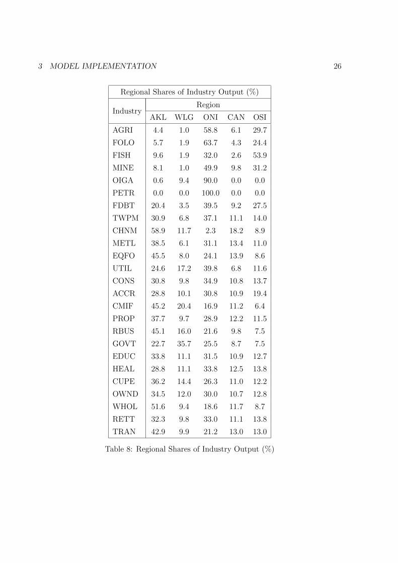
3.1 Benchmark Equilibrium
The MRIO matrix is derived from a national input-output table and estimates of industry
contributions to regional GDP.17 The regional shares data is shown in table 8. Both the
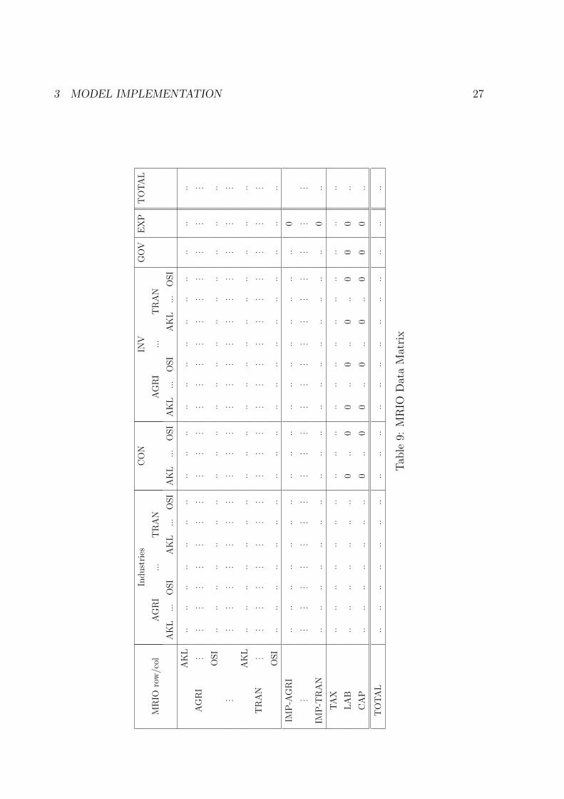
national and multi-regional input-output data tables are very large and therefore omitted.
They are available in Robson (2012). A schematic view of the MRIO is shown in table 9.
McDougall (1999) demonstrates that biproportional allocation is a maximum entropy
solution to the matrix-filling problem. In other words, if we have estimates of the row
and column totals of a matrix M but no other information, then an entropy-maximising
solution is:
M(row , col) =M(row ,TOTAL)×M(TOTAL, col)
M(TOTAL,TOTAL)∀row , col (46)
Defining R(row) = M(row ,TOTAL)M(TOTAL,TOTAL)
and C(col) = M(TOTAL,col)M(TOTAL,TOTAL)
, this can be written as:
M(row , col) = R(row)× C(col)×M(TOTAL,TOTAL) ∀row , col
An entropy-maximising regional split of a cell of the national input-output table, IO(row , col),
can be obtained with regional shares of the flow to col (source shares) and regional shares
of the flow from row (destination shares).
17These items were adapted from data provided by Business and Economics Limited (BERL), an
economics consultancy based in Wellington, New Zealand.
3 MODEL IMPLEMENTATION 25
Label Description
AGRI Agriculture
FOLO Forestry and logging
FISH Fishing
MINE Mining and quarrying
OIGA Oil and gas
PETR Refined petrol
FDBT Food, beverages, and tobacco
TWPM Textiles, wood, paper, and media
CHNM Chemicals and non-metallic minerals
METL Basic and fabricated metal
EQFO Equipment, furniture, and other manufacturing
UTIL Electricity, water, and waste services
CONS Construction
ACCR Accommodation, restaurants, and bars
CMIF Communications, insurance, and finance
PROP Real estate and equipment hire
RBUS Research and business services
GOVT Government administration
EDUC Education
HEAL Health
CUPE Cultural and personal services
OWND Ownership of owner-occupied dwellings
WHOL Wholesale trade
RETT Retail trade
TRAN Transport
Table 7: Industries
3 MODEL IMPLEMENTATION 26
Regional Shares of Industry Output (%)
IndustryRegion
AKL WLG ONI CAN OSI
AGRI 4.4 1.0 58.8 6.1 29.7
FOLO 5.7 1.9 63.7 4.3 24.4
FISH 9.6 1.9 32.0 2.6 53.9
MINE 8.1 1.0 49.9 9.8 31.2
OIGA 0.6 9.4 90.0 0.0 0.0
PETR 0.0 0.0 100.0 0.0 0.0
FDBT 20.4 3.5 39.5 9.2 27.5
TWPM 30.9 6.8 37.1 11.1 14.0
CHNM 58.9 11.7 2.3 18.2 8.9
METL 38.5 6.1 31.1 13.4 11.0
EQFO 45.5 8.0 24.1 13.9 8.6
UTIL 24.6 17.2 39.8 6.8 11.6
CONS 30.8 9.8 34.9 10.8 13.7
ACCR 28.8 10.1 30.8 10.9 19.4
CMIF 45.2 20.4 16.9 11.2 6.4
PROP 37.7 9.7 28.9 12.2 11.5
RBUS 45.1 16.0 21.6 9.8 7.5
GOVT 22.7 35.7 25.5 8.7 7.5
EDUC 33.8 11.1 31.5 10.9 12.7
HEAL 28.8 11.1 33.8 12.5 13.8
CUPE 36.2 14.4 26.3 11.0 12.2
OWND 34.5 12.0 30.0 10.7 12.8
WHOL 51.6 9.4 18.6 11.7 8.7
RETT 32.3 9.8 33.0 11.1 13.8
TRAN 42.9 9.9 21.2 13.0 13.0
Table 8: Regional Shares of Industry Output (%)
3 MODEL IMPLEMENTATION 27
MR
IOro
w/c
ol
Indust
ries
CO
NIN
VG
OV
EX
PT
OT
AL
AG
RI
...
TR
AN
AG
RI
...
TR
AN
AK
L...
OSI
AK
L...
OSI
AK
L...
OSI
AK
L...
OSI
AK
L...
OSI
AG
RI
AK
L..
....
....
....
....
....
....
....
....
....
... . .
. . .. . .
. . .. . .
. . .. . .
. . .. . .
. . .. . .
. . .. . .
. . .. . .
. . .. . .
. . .. . .
. . .. . .
OSI
....
....
....
....
....
....
....
....
....
....
. . .. . .
. . .. . .
. . .. . .
. . .. . .
. . .. . .
. . .. . .
. . .. . .
. . .. . .
. . .. . .
. . .. . .
. . .
TR
AN
AK
L..
....
....
....
....
....
....
....
....
....
... . .
. . .. . .
. . .. . .
. . .. . .
. . .. . .
. . .. . .
. . .. . .
. . .. . .
. . .. . .
. . .. . .
. . .. . .
OSI
....
....
....
....
....
....
....
....
....
....
IMP
-AG
RI
....
....
....
....
....
....
....
....
....
0. . .
. . .. . .
. . .. . .
. . .. . .
. . .. . .
. . .. . .
. . .. . .
. . .. . .
. . .. . .
. . .. . .
. . .. . .
IMP
-TR
AN
....
....
....
....
....
....
....
....
....
0..
TA
X..
....
....
....
....
....
....
....
....
....
..
LA
B..
....
....
....
0..
00
..0
..0
..0
00
..
CA
P..
....
....
....
0..
00
..0
..0
..0
00
..
TO
TA
L..
....
....
....
....
....
....
....
....
....
..
Tab
le9:
MR
IOD
ata
Mat
rix
3 MODEL IMPLEMENTATION 28
For example, MRIO(g−x,CON−r) — the flow of product g from region x to the
household agent in region r — is estimated as:
MRIO(g−x,CON−r) = [XOUTPUTg,x/g ]× [XLABOUR
r/tot ]× IO(DOM−g,CON)
where [XOUTPUTg,x/g ] is region x’s share of output of g as shown in table 8, and [XLABOUR
r/tot ]
is region r’s employment share.
The other MRIO cells are derived in a similar fashion. This procedure adheres to
principles of information theory so as to not introduce unintended bias in the regional
pattern of trade. Formally, the entropy of the whole MRIO matrix is maximised subject
to the condition that each block adds up to the respective IO table cell.
In cases where we have additional information on regional sources and destinations,
this can be incorporated without disturbing the matrix balance through the use of a
RAS algorithm (which is just the same biproportional allocation technique but applied to
matrix balancing rather than matrix filling). For instance, we may want to assume some
industries are local — they only sell their product to agents in their local region (and
the government and exporters). This assumption is made in this implementation for the
industries listed in table 10.
Adjustments are required to the allocation of IO cell values over the relevant MRIO
blocks to reflect the local product assumption. For example, since the product/industry
EDUC is assumed local, the flows to MRIO column CON-r are specified as:
MRIO(EDUC−x,CON−r) = [XLABOURr/tot ]× IO(DOM− EDUC,CON)× 1
x=r (47)
These kinds of adjustments inevitably disturb the balance of the MRIO matrix. It is
almost certain that the totals of the domestic product rows will no longer equal the totals
of the respective industry columns and the MRIO matrix will not be consistent with
equilibrium. To enforce consistency and restrict the information gain to those parts of
the MRIO matrix that we directly manipulate, we seek a cross-entropy solution to re-
balancing the matrix. Performing a RAS algorithm on the unbalanced MRIO matrix
achieves this: the solution minimises the distance between the MRIO matrix and the
biproportional allocation.18
18The seminal treatment of the RAS method is Bacharach (1970) while McDougall (1999) links the
RAS to cross-entropy.
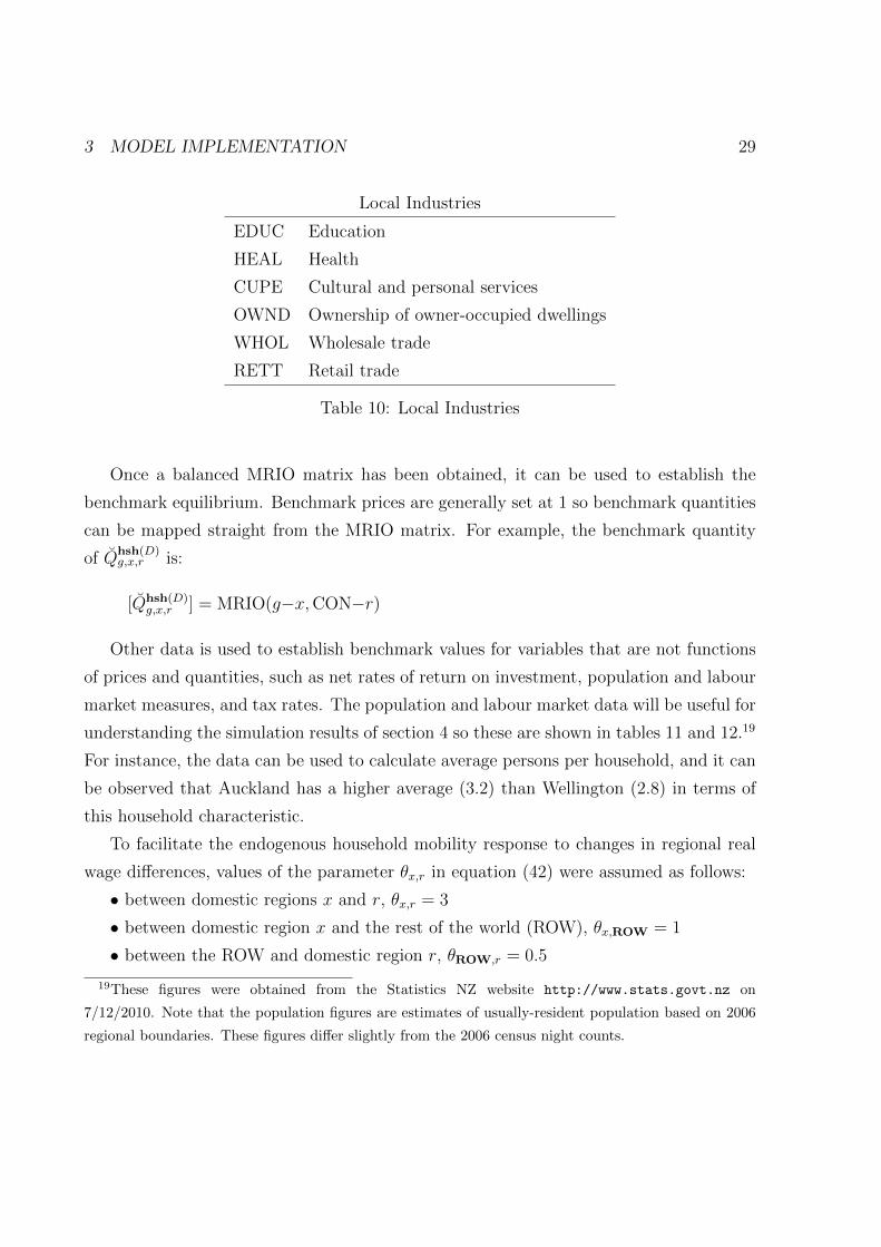
3 MODEL IMPLEMENTATION 29
Local Industries
EDUC Education
HEAL Health
CUPE Cultural and personal services
OWND Ownership of owner-occupied dwellings
WHOL Wholesale trade
RETT Retail trade
Table 10: Local Industries
Once a balanced MRIO matrix has been obtained, it can be used to establish the
benchmark equilibrium. Benchmark prices are generally set at 1 so benchmark quantities
can be mapped straight from the MRIO matrix. For example, the benchmark quantity
of Qhsh(D)g,x,r is:
[Qhsh(D)g,x,r ] = MRIO(g−x,CON−r)
Other data is used to establish benchmark values for variables that are not functions
of prices and quantities, such as net rates of return on investment, population and labour
market measures, and tax rates. The population and labour market data will be useful for
understanding the simulation results of section 4 so these are shown in tables 11 and 12.19
For instance, the data can be used to calculate average persons per household, and it can
be observed that Auckland has a higher average (3.2) than Wellington (2.8) in terms of
this household characteristic.
To facilitate the endogenous household mobility response to changes in regional real
wage differences, values of the parameter θx,r in equation (42) were assumed as follows:
• between domestic regions x and r, θx,r = 3
• between domestic region x and the rest of the world (ROW), θx,ROW = 1
• between the ROW and domestic region r, θROW,r = 0.5
19These figures were obtained from the Statistics NZ website http://www.stats.govt.nz on
7/12/2010. Note that the population figures are estimates of usually-resident population based on 2006
regional boundaries. These figures differ slightly from the 2006 census night counts.
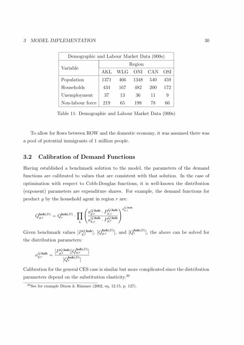
3 MODEL IMPLEMENTATION 30
Demographic and Labour Market Data (000s)
VariableRegion
AKL WLG ONI CAN OSI
Population 1371 466 1348 540 459
Households 434 167 482 200 172
Unemployment 37 13 36 11 9
Non-labour force 219 65 198 78 66
Table 11: Demographic and Labour Market Data (000s)
To allow for flows between ROW and the domestic economy, it was assumed there was
a pool of potential immigrants of 1 million people.
3.2 Calibration of Demand Functions
Having established a benchmark solution to the model, the parameters of the demand
functions are calibrated to values that are consistent with that solution. In the case of
optimisation with respect to Cobb-Douglas functions, it is well-known the distribution
(exponent) parameters are expenditure shares. For example, the demand functions for
product g by the household agent in region r are:
Qhsh(D)g,r = Qhsh(D)
r ·∏h
(aQ,hshg,r · PQ,hsh
h,r
aQ,hshh,r · PQ,hshg,r
)aQ,hshh,r
Given benchmark values [PQ,hshg,r ], [Q
hsh(D)g,r ], and [Q
hsh(D)r ], the above can be solved for
the distribution parameters:
aQ,hshg,r =[PQ,hshg,r ][Q
hsh(D)g,r ]
[Qhsh(D)r ]
Calibration for the general CES case is similar but more complicated since the distribution
parameters depend on the substitution elasticity.20
20See for example Dixon & Rimmer (2002, eq. 12.15, p. 127).
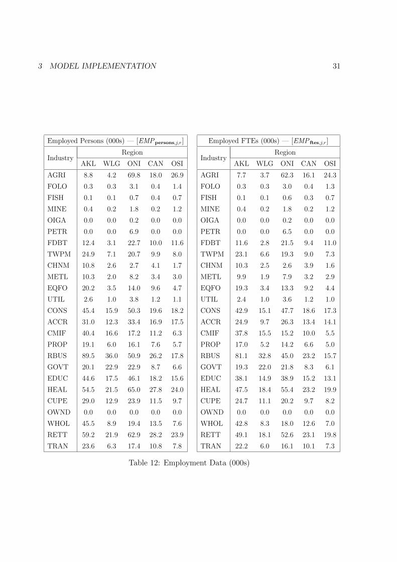
3 MODEL IMPLEMENTATION 31
Employed Persons (000s) — [EMPpersons,j,r]
IndustryRegion
AKL WLG ONI CAN OSI
AGRI 8.8 4.2 69.8 18.0 26.9
FOLO 0.3 0.3 3.1 0.4 1.4
FISH 0.1 0.1 0.7 0.4 0.7
MINE 0.4 0.2 1.8 0.2 1.2
OIGA 0.0 0.0 0.2 0.0 0.0
PETR 0.0 0.0 6.9 0.0 0.0
FDBT 12.4 3.1 22.7 10.0 11.6
TWPM 24.9 7.1 20.7 9.9 8.0
CHNM 10.8 2.6 2.7 4.1 1.7
METL 10.3 2.0 8.2 3.4 3.0
EQFO 20.2 3.5 14.0 9.6 4.7
UTIL 2.6 1.0 3.8 1.2 1.1
CONS 45.4 15.9 50.3 19.6 18.2
ACCR 31.0 12.3 33.4 16.9 17.5
CMIF 40.4 16.6 17.2 11.2 6.3
PROP 19.1 6.0 16.1 7.6 5.7
RBUS 89.5 36.0 50.9 26.2 17.8
GOVT 20.1 22.9 22.9 8.7 6.6
EDUC 44.6 17.5 46.1 18.2 15.6
HEAL 54.5 21.5 65.0 27.8 24.0
CUPE 29.0 12.9 23.9 11.5 9.7
OWND 0.0 0.0 0.0 0.0 0.0
WHOL 45.5 8.9 19.4 13.5 7.6
RETT 59.2 21.9 62.9 28.2 23.9
TRAN 23.6 6.3 17.4 10.8 7.8
Employed FTEs (000s) — [EMP ftes,j,r]
IndustryRegion
AKL WLG ONI CAN OSI
AGRI 7.7 3.7 62.3 16.1 24.3
FOLO 0.3 0.3 3.0 0.4 1.3
FISH 0.1 0.1 0.6 0.3 0.7
MINE 0.4 0.2 1.8 0.2 1.2
OIGA 0.0 0.0 0.2 0.0 0.0
PETR 0.0 0.0 6.5 0.0 0.0
FDBT 11.6 2.8 21.5 9.4 11.0
TWPM 23.1 6.6 19.3 9.0 7.3
CHNM 10.3 2.5 2.6 3.9 1.6
METL 9.9 1.9 7.9 3.2 2.9
EQFO 19.3 3.4 13.3 9.2 4.4
UTIL 2.4 1.0 3.6 1.2 1.0
CONS 42.9 15.1 47.7 18.6 17.3
ACCR 24.9 9.7 26.3 13.4 14.1
CMIF 37.8 15.5 15.2 10.0 5.5
PROP 17.0 5.2 14.2 6.6 5.0
RBUS 81.1 32.8 45.0 23.2 15.7
GOVT 19.3 22.0 21.8 8.3 6.1
EDUC 38.1 14.9 38.9 15.2 13.1
HEAL 47.5 18.4 55.4 23.2 19.9
CUPE 24.7 11.1 20.2 9.7 8.2
OWND 0.0 0.0 0.0 0.0 0.0
WHOL 42.8 8.3 18.0 12.6 7.0
RETT 49.1 18.1 52.6 23.1 19.8
TRAN 22.2 6.0 16.1 10.1 7.3
Table 12: Employment Data (000s)
3 MODEL IMPLEMENTATION 32
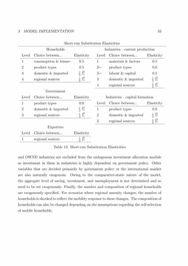
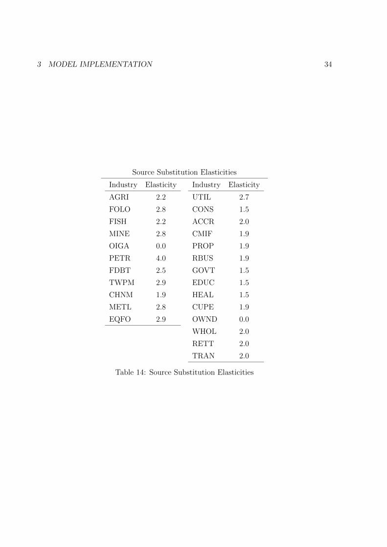
Substitution elasticity values were adopted based on international practice and New
Zealand estimates where available. The assumed elasticities are shown in table 13 where
~Σ is a vector of source substitution elasticities shown in table 14.21 This vector is scaled
up or down to reflect a short-run or long-run simulation mode, to reflect that agents are
more willing and able to substitute between regional varieties than between the domestic
and foreign varieties, and for sensitivity analysis. The particular scaling shown in table
13 represent a low level of relative price sensitivity in the short-run.
The calibration of the margin demand functions for distribution services — equation
(38) — ensures that assumptions made when formulating the benchmark equilibrium
regarding how the services are used to deliver products are reflected in the structure of
aQ,agentm,y,g,s . Specific assumptions made regarding distribution services in this implementation
include that retail services are only used for delivering products to local agents and that
transport services are only used as margins for delivering products between regions, not
within regions. Wholesale and retail services are associated with demands in destinations
while transport services are associated with supplies from sources. The vQ,agentg,s parameters
in equation (38) capture the commodity tax component of delivered products. For further
details on how the distribution services modelling is implemented in JENNIFER, see
Robson (2012, chapter 3).
3.3 Model Closure
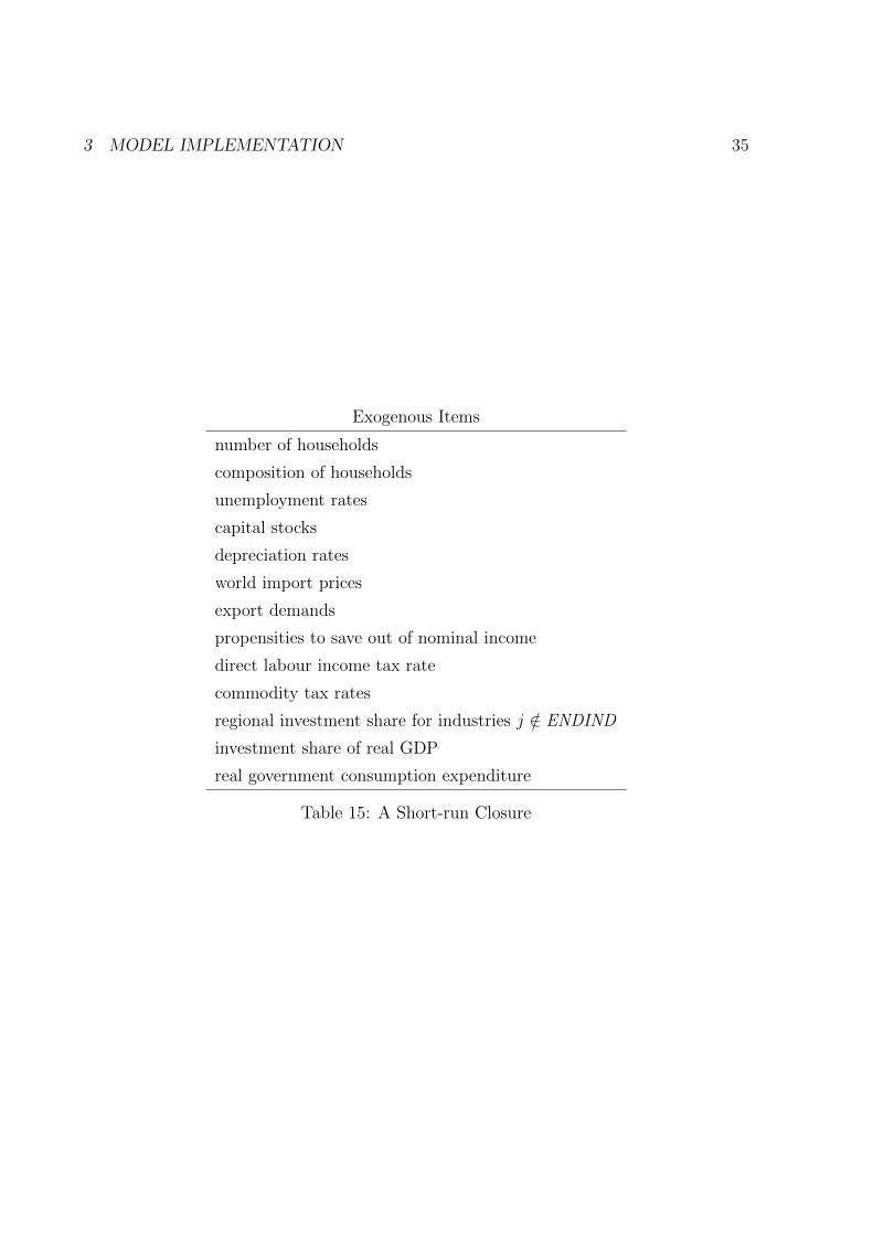
As the model involves more variables than explaining equations, an additional set of
equations are required to fix the appropriate number of variables exogenously so that
the model becomes a square system. The closure choice is important because simulation
results can only be interpreted with respect to that choice. A typical short-run closure
for the model is shown in table 15, and this is the closure used for our simulations in
section 4. The closure is interpreted as short-run because the endowments of capital are
fixed — capital is not free to move between regions or industries to seek out the best rate
of return. The only response to a change in relative rates of return is a reallocation of
the investment budget. In the 25-industry implementation, the GOVT, EDUC, HEAL,
21These elasticities were adapted from data provided by Business and Economics Limited (BERL), an
economics consultancy based in Wellington, New Zealand.
3 MODEL IMPLEMENTATION 33
Short-run Substitution Elasticities
Households
Level Choice between... Elasticity
1 consumption & leisure 0.5
2 product types 0.5
3 domestic & imported 13~Σ
4 regional sources 12~Σ
Government
Level Choice between... Elasticity
1 product types 0.0
2 domestic & imported 14~Σ
3 regional sources 13~Σ
Exporters
Level Choice between... Elasticity
1 regional sources 12~Σ
Industries - current production
Level Choice between... Elasticity
1 materials & factors 0.5
2= product types 0.0
2= labour & capital 0.5
3 domestic & imported 13~Σ
4 regional sources 12~Σ
Industries - capital formation
Level Choice between... Elasticity
1 product types 0.0
2 domestic & imported 13~Σ
3 regional sources 12~Σ
Table 13: Short-run Substitution Elasticities
and OWND industries are excluded from the endogenous investment allocation module
as investment in these in industries is highly dependent on government policy. Other
variables that are decided primarily by government policy or the international market
are also naturally exogenous. Owing to the comparative-static nature of the model,
the aggregate level of saving, investment, and unemployment is not determined and so
need to be set exogenously. Finally, the number and composition of regional households
are exogenously specified. For scenarios where regional amenity changes, the number of
households is shocked to reflect the mobility response to these changes. The composition of
households can also be changed depending on the assumptions regarding the self-selection
of mobile households.
3 MODEL IMPLEMENTATION 34
Source Substitution Elasticities
Industry Elasticity
AGRI 2.2
FOLO 2.8
FISH 2.2
MINE 2.8
OIGA 0.0
PETR 4.0
FDBT 2.5
TWPM 2.9
CHNM 1.9
METL 2.8
EQFO 2.9
Industry Elasticity
UTIL 2.7
CONS 1.5
ACCR 2.0
CMIF 1.9
PROP 1.9
RBUS 1.9
GOVT 1.5
EDUC 1.5
HEAL 1.5
CUPE 1.9
OWND 0.0
WHOL 2.0
RETT 2.0
TRAN 2.0
Table 14: Source Substitution Elasticities
3 MODEL IMPLEMENTATION 35
Exogenous Items
number of households
composition of households
unemployment rates
capital stocks
depreciation rates
world import prices
export demands
propensities to save out of nominal income
direct labour income tax rate
commodity tax rates
regional investment share for industries j /∈ ENDIND
investment share of real GDP
real government consumption expenditure
Table 15: A Short-run Closure
4 AN ILLUSTRATIVE APPLICATION 36
4 An Illustrative Application
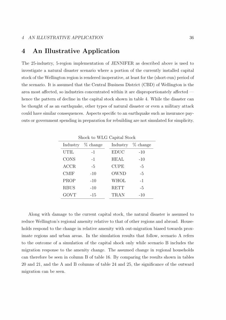
The 25-industry, 5-region implementation of JENNIFER as described above is used to
investigate a natural disaster scenario where a portion of the currently installed capital
stock of the Wellington region is rendered inoperative, at least for the (short-run) period of
the scenario. It is assumed that the Central Business District (CBD) of Wellington is the
area most affected, so industries concentrated within it are disproportionately affected —
hence the pattern of decline in the capital stock shown in table 4. While the disaster can
be thought of as an earthquake, other types of natural disaster or even a military attack
could have similar consequences. Aspects specific to an earthquake such as insurance pay-
outs or government spending in preparation for rebuilding are not simulated for simplicity.
Shock to WLG Capital Stock
Industry % change
UTIL -1
CONS -1
ACCR -5
CMIF -10
PROP -10
RBUS -10
GOVT -15
Industry % change
EDUC -10
HEAL -10
CUPE -5
OWND -5
WHOL -1
RETT -5
TRAN -10
Along with damage to the current capital stock, the natural disaster is assumed to
reduce Wellington’s regional amenity relative to that of other regions and abroad. House-
holds respond to the change in relative amenity with out-migration biased towards prox-
imate regions and urban areas. In the simulation results that follow, scenario A refers
to the outcome of a simulation of the capital shock only while scenario B includes the
migration response to the amenity change. The assumed change in regional households
can therefore be seen in column B of table 16. By comparing the results shown in tables
20 and 21, and the A and B columns of table 24 and 25, the significance of the outward
migration can be seen.
4 AN ILLUSTRATIVE APPLICATION 37
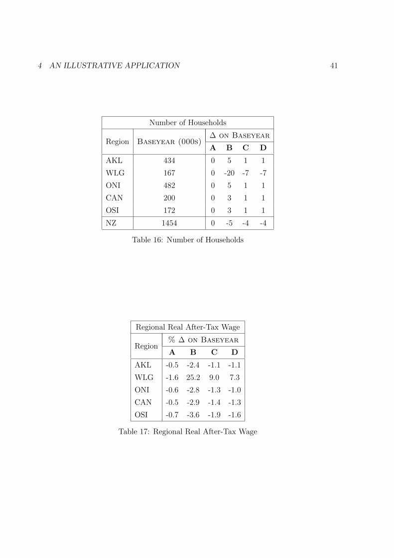
Scenario C adds in the endogenous migration response to the regional wage differences
calculated in scenario B, as shown in table 17. Due to its relatively higher real wage
rate, households from other regions and abroad flow into Wellington, as seen in table
18. This partially offsets the initial outflow due to the loss of regional amenity, so the
migration pattern is less pronounced — compare columns B and C in table 16. As
household characteristics such as the working age / non-working age composition differ
across regions, the migration flows cause changes in Wellington’s average characteristics.
To see the extent that the composition effects impact the results, scenario D repeats the
same shock to regional households as scenario C, but without the change in household
characteristics associated with the inward migration. Thus it can be seen from tables 22
and 23 that scenario C includes an increase in non-working age persons per household,
for example, while scenario D excludes this change.
The following discussion highlights a range of insights we can take from these simula-
tion results.
Aggregate supply shock At the national level, the loss of current capital has the
hallmarks of a classical aggregate supply shock — output falls and prices rise — in all the
scenarios (table 24). Household consumption and saving fall due to the loss of capital in-
come and investment falls in line with GDP by assumption. With no change in government
spending, the trade balance must decline more than proportionately for macroeconomic
balance. Domestic prices rise relative to foreign prices so there is some substitution to-
wards imported products but overall imports falls. A more than proportionate fall is
exports is therefore required. From the perspective of foreign borrowing requirements,
the decline in the government budget surplus (due to a fall in tax revenue) and household
saving will mean an increase in national debt is required to support investment and the
larger trade deficit.
Different impacts across regions While the shock has a relatively minor effect at the
national level, the regions experience quite different outcomes. For these scenarios where
the shock originates in one region only, the impact on that region stands in contrast to
all the others. In scenario A for example, real household consumption rises in Wellington
while it falls elsewhere (table 20). The sudden shortage of capital in Wellington drives

4 AN ILLUSTRATIVE APPLICATION 38
up rental rates (table 26) and the overall effect on nominal household income is positive.
Due to the assumption that nominal consumption moves in line with nominal income, and
since the rise in the regional consumption price index is less than the increase in nominal
income, real consumption must rise even though real income has fallen. This translates
to a substantial fall in real household saving in Wellington. The higher rental rates on
capital in Wellington lead to higher output prices for Wellington products, which increase
production costs and therefore output prices elsewhere. With no significant change in
real disposable income and higher consumption prices, real consumption falls in regions
outside Wellington.
Household outflows exacerbate the shock The negative aspects of the shock are
roughly doubled at the national level and tripled for Wellington when household out-
migration as shown in column B of table 16 is added to the scenario to take into account
the loss of regional amenity due to the disaster. Aggregate real GDP falls 0.8% in scenario
B compared to 0.4% in scenario A, while Wellington’s real GDP falls 6.1% rather than
1.9% (table 21). The fall in labour supply in Wellington means less regional income and
a higher wage rate. Faced with weak regional demand and higher factor costs, firms cut
back production more than in scenario A. Although the price of Wellington products is
much higher, the other regions are not adversely affected — with inflows of labour from
Wellington driving down their wage rates, the other regions see smaller rises in produc-
tion costs and do not have to decrease output as much. The fixed average consumption
propensity again means Wellington’s real consumption increases, and interestingly, more
than in scenario A, even with less regional households. Real consumption spending per
Wellington household increases significantly in scenario B but without a commensurate
increase in disposable income, this increase comes from a very large decrease in saving
per household (table 25). The other regions have the opposite outcome — with a similar
level of regional disposable income to that of scenario A but more households, income and
spending per household is lower in scenario B. These outcomes are reflected in the real
regional GDP per capita results, with Wellington actually seeing an increase in GDP per
capita.
4 AN ILLUSTRATIVE APPLICATION 39
... But sensitivity to regional real wage differences moderates the impact One
outcome of scenario B is that the real wage rate in Wellington increases by 25% while
those in other regions fall (table 17). It is unrealistic that such a gap between the regional
returns to labour remains in equilibrium, even in the short-run. Scenario C adjusts the
household outflow to take into account in-migration of households in response to the
higher real wage rate on offer in Wellington. The net outflow therefore is much lower
than in scenario B, as seen in table 16. In terms of the aggregate and key regional results,
scenario C is an intermediate case between scenarios A and B. The sign on most of the
results for scenario C is the same as for scenario B, but the magnitudes are lower. Gross
investment is one exception: while in scenario B investment in Wellington fell roughly in
line with other regions, in scenario C it saw a small increase in investment, against falls
elsewhere. This is partly the result of Wellington being allocated more of the investment
budget due to better rates of return outcomes and partly because overall the investment
budget is larger. In Wellington, most of those industries for which investment is allocated
endogenously see smaller falls in investment in scenario C (table 29) while the results for
Auckland were roughly the same between scenarios B and C (table 28). This is due to
lower capital construction costs in Wellington giving rise to higher net rates of return to
those industries in scenario C (table 27). Also, recall that the GOVT, EDUC, HEAL,
and OWND industries are not subject to endogenous investment allocation. Instead, their
share of the investment budget is set exogenous so they move in line with aggregate real
investment. In scenario C, aggregate investment falls less than in scenario B so investment
in these industries changes likewise. The lower capital construction costs can be traced
back to the dampened rise in the wage rate (due to the endogenous household migration
response) via the lower input prices to capital formation.
Composition effects are important for labour market outcomes It is noticeable
from table 22 that the household inflows resulting from a higher real wage in Welling-
ton change the average composition of households in that region, while the outflows from
Wellington due to the amenity loss affect the average composition of other regions, partic-
ularly those in the North Island. Wellington ends up with a higher number of persons per
household, especially of non-working age. With employment falling, there is also a shift

4 AN ILLUSTRATIVE APPLICATION 40
to non-labour force activity — the participation rate in Wellington falls 1.4 percentage
points to 77% (table 19). The way these composition effects are calculated is by assuming
that Wellington households are only sensitive to the amenity change while out-of-region
households are only sensitive to the relative real wage rate differences. We may wish to
consider the case where the higher real wage encourages some Wellington households to
remain when otherwise they would have left — then the composition effects would not be
as pronounced. For this purpose, the results of scenario D are included for comparison.
In this scenario the same net outflow of households is assumed as in scenario C (and the
capital shock) but the composition effects are calculated as though the net outflow is also
the gross flow — there are no households migrating to Wellington thereby affecting the
average household composition. Comparing the results for Wellington in tables 22 and
23, and the C and D columns of table 19, it can be seen that the composition changes
included in scenario C reduce employment by about one percentage point and the labour
force participation rate by about 0.7 percentage points. Regional real GDP per capita is
also reduced by 0.6 percentage points due to the composition effects. This comparison is
also useful as scenario C can also be interpreted as the outcome of biased self-selection
of migrating Wellington households. If those households leaving Wellington are typically
smaller and with less dependents than those staying (for example, young single profession-
als versus established families with school-aged children), the composition effects would
be similar to those of scenario C. Then a comparison with scenario D (where self-selection
is not biased) informs on the impact of that biased self-selection, an analysis of which
may be of interest to policymakers following the disaster.
Further results from these scenarios are available from the author on request. The
industry-by-region breakdown of gross output and employment effects, and changes to
various macro price indices are provided in appendix C for the interested reader.
4 AN ILLUSTRATIVE APPLICATION 41
Number of Households
Region Baseyear (000s)∆ on Baseyear
A B C D
AKL 434 0 5 1 1
WLG 167 0 -20 -7 -7
ONI 482 0 5 1 1
CAN 200 0 3 1 1
OSI 172 0 3 1 1
NZ 1454 0 -5 -4 -4
Table 16: Number of Households
Regional Real After-Tax Wage
Region% ∆ on Baseyear
A B C D
AKL -0.5 -2.4 -1.1 -1.1
WLG -1.6 25.2 9.0 7.3
ONI -0.6 -2.8 -1.3 -1.0
CAN -0.5 -2.9 -1.4 -1.3
OSI -0.7 -3.6 -1.9 -1.6
Table 17: Regional Real After-Tax Wage
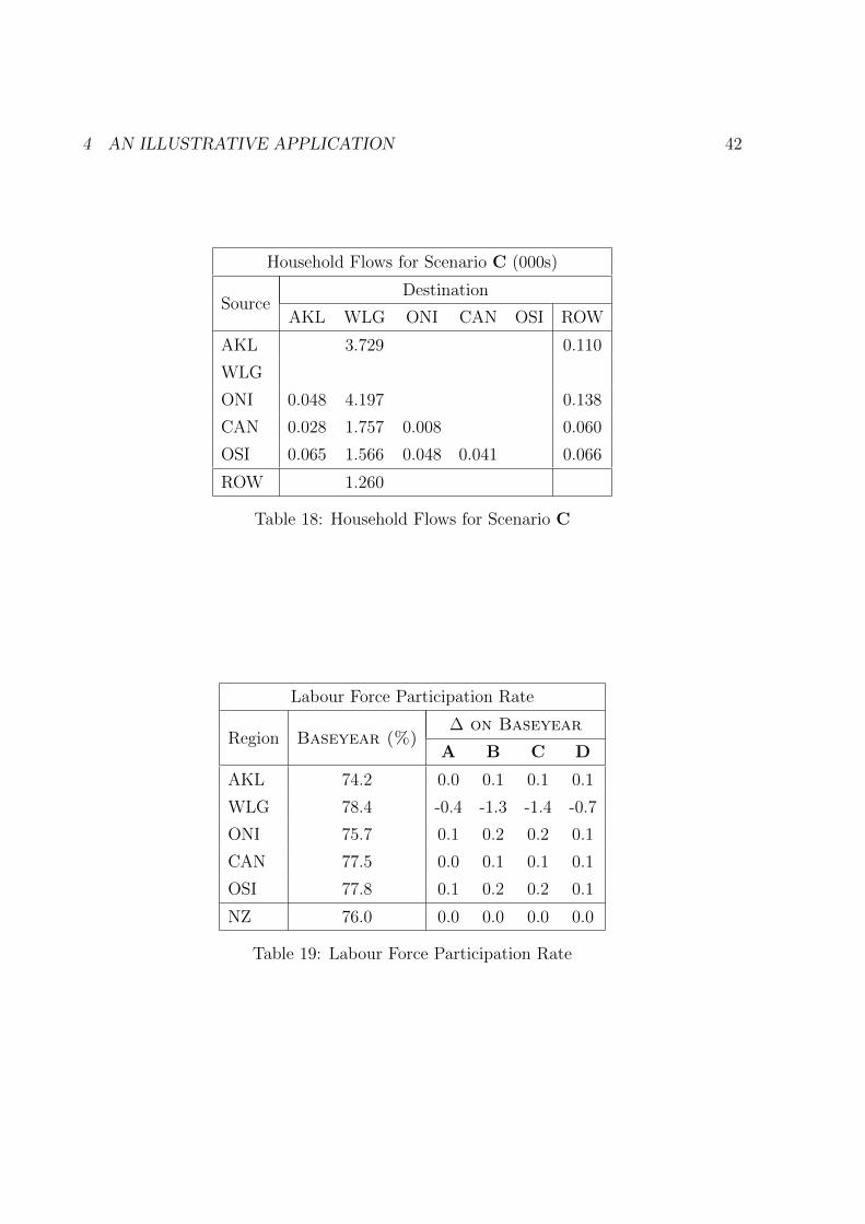
4 AN ILLUSTRATIVE APPLICATION 42
Household Flows for Scenario C (000s)
SourceDestination
AKL WLG ONI CAN OSI ROW
AKL 3.729 0.110
WLG
ONI 0.048 4.197 0.138
CAN 0.028 1.757 0.008 0.060
OSI 0.065 1.566 0.048 0.041 0.066
ROW 1.260
Table 18: Household Flows for Scenario C
Labour Force Participation Rate
Region Baseyear (%)∆ on Baseyear
A B C D
AKL 74.2 0.0 0.1 0.1 0.1
WLG 78.4 -0.4 -1.3 -1.4 -0.7
ONI 75.7 0.1 0.2 0.2 0.1
CAN 77.5 0.0 0.1 0.1 0.1
OSI 77.8 0.1 0.2 0.2 0.1
NZ 76.0 0.0 0.0 0.0 0.0
Table 19: Labour Force Participation Rate

4 AN ILLUSTRATIVE APPLICATION 43
Key Results — Scenario A
Variable% ∆ on Baseyear
AKL WLG ONI CAN OSI NZ
Real GDP (expenditure) -0.3 -1.9 -0.2 -0.2 -0.2 -0.4
Real GDP per capita -0.3 -1.9 -0.2 -0.2 -0.2 -0.4
Gross output -0.2 -2.0 -0.2 -0.2 -0.2 -0.4
Gross investment -0.6 0.9 -0.7 -0.6 -0.7 -0.4
Disposable income 0.0 -3.8 0.0 0.0 0.0 -0.4
Private consumption -0.4 1.1 -0.6 -0.4 -0.6 -0.3
Private saving 1.5 -23.1 1.9 1.7 2.6 -1.0
Working age population 0.0 0.0 0.0 0.0 0.0 0.0
Non-working age population 0.0 0.0 0.0 0.0 0.0 0.0
Total population 0.0 0.0 0.0 0.0 0.0 0.0
Total households 0.0 0.0 0.0 0.0 0.0 0.0
Employment 0.1 -0.5 0.1 0.1 0.1 0.0
Unemployment 0.1 -0.5 0.1 0.1 0.1 0.0
Non-labour force -0.2 1.9 -0.2 -0.2 -0.3 0.0
Capital Stocks 0.0 -8.2 0.0 0.0 0.0 -1.1
Consumption price deflator 0.3 2.7 0.2 0.3 0.2 0.5
Real after-tax wage rate -0.5 -1.6 -0.6 -0.5 -0.7 -0.7
Output price deflator 0.2 3.8 0.1 0.2 0.0 0.5
Investment net rate of return -0.3 24.4 -0.7 -0.5 -0.8 2.3
Table 20: Key Results — Scenario A
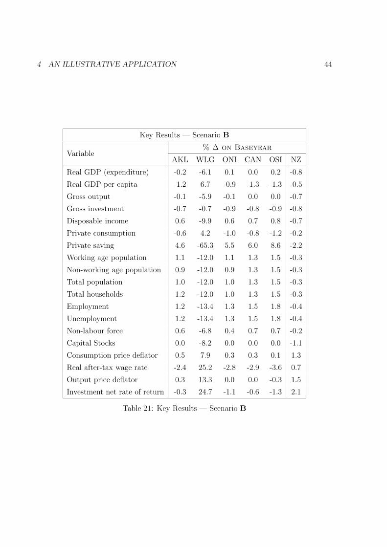
4 AN ILLUSTRATIVE APPLICATION 44
Key Results — Scenario B
Variable% ∆ on Baseyear
AKL WLG ONI CAN OSI NZ
Real GDP (expenditure) -0.2 -6.1 0.1 0.0 0.2 -0.8
Real GDP per capita -1.2 6.7 -0.9 -1.3 -1.3 -0.5
Gross output -0.1 -5.9 -0.1 0.0 0.0 -0.7
Gross investment -0.7 -0.7 -0.9 -0.8 -0.9 -0.8
Disposable income 0.6 -9.9 0.6 0.7 0.8 -0.7
Private consumption -0.6 4.2 -1.0 -0.8 -1.2 -0.2
Private saving 4.6 -65.3 5.5 6.0 8.6 -2.2
Working age population 1.1 -12.0 1.1 1.3 1.5 -0.3
Non-working age population 0.9 -12.0 0.9 1.3 1.5 -0.3
Total population 1.0 -12.0 1.0 1.3 1.5 -0.3
Total households 1.2 -12.0 1.0 1.3 1.5 -0.3
Employment 1.2 -13.4 1.3 1.5 1.8 -0.4
Unemployment 1.2 -13.4 1.3 1.5 1.8 -0.4
Non-labour force 0.6 -6.8 0.4 0.7 0.7 -0.2
Capital Stocks 0.0 -8.2 0.0 0.0 0.0 -1.1
Consumption price deflator 0.5 7.9 0.3 0.3 0.1 1.3
Real after-tax wage rate -2.4 25.2 -2.8 -2.9 -3.6 0.7
Output price deflator 0.3 13.3 0.0 0.0 -0.3 1.5
Investment net rate of return -0.3 24.7 -1.1 -0.6 -1.3 2.1
Table 21: Key Results — Scenario B
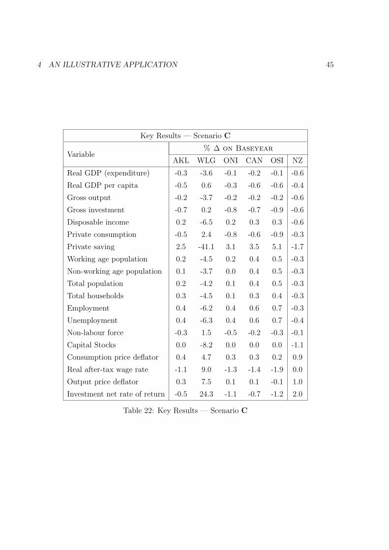
4 AN ILLUSTRATIVE APPLICATION 45
Key Results — Scenario C
Variable% ∆ on Baseyear
AKL WLG ONI CAN OSI NZ
Real GDP (expenditure) -0.3 -3.6 -0.1 -0.2 -0.1 -0.6
Real GDP per capita -0.5 0.6 -0.3 -0.6 -0.6 -0.4
Gross output -0.2 -3.7 -0.2 -0.2 -0.2 -0.6
Gross investment -0.7 0.2 -0.8 -0.7 -0.9 -0.6
Disposable income 0.2 -6.5 0.2 0.3 0.3 -0.6
Private consumption -0.5 2.4 -0.8 -0.6 -0.9 -0.3
Private saving 2.5 -41.1 3.1 3.5 5.1 -1.7
Working age population 0.2 -4.5 0.2 0.4 0.5 -0.3
Non-working age population 0.1 -3.7 0.0 0.4 0.5 -0.3
Total population 0.2 -4.2 0.1 0.4 0.5 -0.3
Total households 0.3 -4.5 0.1 0.3 0.4 -0.3
Employment 0.4 -6.2 0.4 0.6 0.7 -0.3
Unemployment 0.4 -6.3 0.4 0.6 0.7 -0.4
Non-labour force -0.3 1.5 -0.5 -0.2 -0.3 -0.1
Capital Stocks 0.0 -8.2 0.0 0.0 0.0 -1.1
Consumption price deflator 0.4 4.7 0.3 0.3 0.2 0.9
Real after-tax wage rate -1.1 9.0 -1.3 -1.4 -1.9 0.0
Output price deflator 0.3 7.5 0.1 0.1 -0.1 1.0
Investment net rate of return -0.5 24.3 -1.1 -0.7 -1.2 2.0
Table 22: Key Results — Scenario C

4 AN ILLUSTRATIVE APPLICATION 46
Key Results — Scenario D
Variable% ∆ on Baseyear
AKL WLG ONI CAN OSI NZ
Real GDP (expenditure) -0.3 -3.4 -0.2 -0.2 -0.1 -0.6
Real GDP per capita -0.6 1.2 -0.3 -0.6 -0.6 -0.3
Gross output -0.2 -3.4 -0.3 -0.2 -0.2 -0.6
Gross investment -0.7 0.3 -0.8 -0.7 -0.9 -0.6
Disposable income 0.2 -6.1 0.1 0.2 0.3 -0.6
Private consumption -0.5 2.2 -0.7 -0.6 -0.9 -0.3
Private saving 2.5 -38.4 2.7 3.2 4.6 -1.6
Working age population 0.3 -4.5 0.1 0.4 0.4 -0.3
Non-working age population 0.2 -4.5 0.1 0.4 0.4 -0.3
Total population 0.3 -4.5 0.1 0.4 0.4 -0.3
Total households 0.3 -4.5 0.1 0.3 0.4 -0.3
Employment 0.4 -5.3 0.3 0.5 0.6 -0.3
Unemployment 0.4 -5.3 0.3 0.5 0.6 -0.3
Non-labour force 0.0 -1.4 -0.2 0.0 0.0 -0.2
Capital Stocks 0.0 -8.2 0.0 0.0 0.0 -1.1
Consumption price deflator 0.3 4.4 0.3 0.3 0.2 0.8
Real after-tax wage rate -1.1 7.3 -1.0 -1.3 -1.6 -0.1
Output price deflator 0.3 6.9 0.1 0.1 -0.1 0.9
Investment net rate of return -0.5 24.3 -1.0 -0.7 -1.2 2.0
Table 23: Key Results — Scenario D
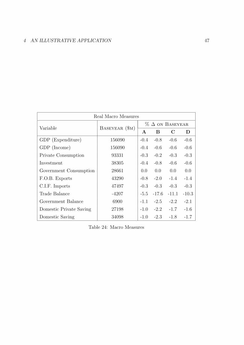
4 AN ILLUSTRATIVE APPLICATION 47
Real Macro Measures
Variable Baseyear ($m)% ∆ on Baseyear
A B C D
GDP (Expenditure) 156090 -0.4 -0.8 -0.6 -0.6
GDP (Income) 156090 -0.4 -0.6 -0.6 -0.6
Private Consumption 93331 -0.3 -0.2 -0.3 -0.3
Investment 38305 -0.4 -0.8 -0.6 -0.6
Government Consumption 28661 0.0 0.0 0.0 0.0
F.O.B. Exports 43290 -0.8 -2.0 -1.4 -1.4
C.I.F. Imports 47497 -0.3 -0.3 -0.3 -0.3
Trade Balance -4207 -5.5 -17.6 -11.1 -10.3
Government Balance 6900 -1.1 -2.5 -2.2 -2.1
Domestic Private Saving 27198 -1.0 -2.2 -1.7 -1.6
Domestic Saving 34098 -1.0 -2.3 -1.8 -1.7
Table 24: Macro Measures
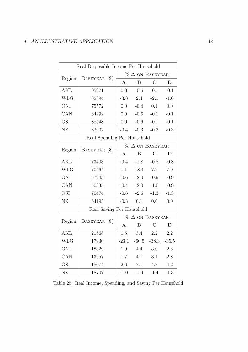
4 AN ILLUSTRATIVE APPLICATION 48
Real Disposable Income Per Household
Region Baseyear ($)% ∆ on Baseyear
A B C D
AKL 95271 0.0 -0.6 -0.1 -0.1
WLG 88394 -3.8 2.4 -2.1 -1.6
ONI 75572 0.0 -0.4 0.1 0.0
CAN 64292 0.0 -0.6 -0.1 -0.1
OSI 88548 0.0 -0.6 -0.1 -0.1
NZ 82902 -0.4 -0.3 -0.3 -0.3
Real Spending Per Household
Region Baseyear ($)% ∆ on Baseyear
A B C D
AKL 73403 -0.4 -1.8 -0.8 -0.8
WLG 70464 1.1 18.4 7.2 7.0
ONI 57243 -0.6 -2.0 -0.9 -0.9
CAN 50335 -0.4 -2.0 -1.0 -0.9
OSI 70474 -0.6 -2.6 -1.3 -1.3
NZ 64195 -0.3 0.1 0.0 0.0
Real Saving Per Household
Region Baseyear ($)% ∆ on Baseyear
A B C D
AKL 21868 1.5 3.4 2.2 2.2
WLG 17930 -23.1 -60.5 -38.3 -35.5
ONI 18329 1.9 4.4 3.0 2.6
CAN 13957 1.7 4.7 3.1 2.8
OSI 18074 2.6 7.1 4.7 4.2
NZ 18707 -1.0 -1.9 -1.4 -1.3
Table 25: Real Income, Spending, and Saving Per Household
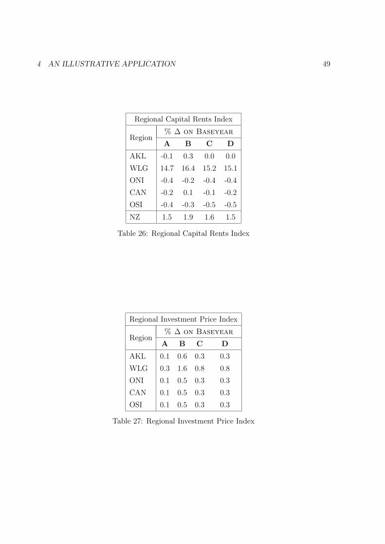
4 AN ILLUSTRATIVE APPLICATION 49
Regional Capital Rents Index
Region% ∆ on Baseyear
A B C D
AKL -0.1 0.3 0.0 0.0
WLG 14.7 16.4 15.2 15.1
ONI -0.4 -0.2 -0.4 -0.4
CAN -0.2 0.1 -0.1 -0.2
OSI -0.4 -0.3 -0.5 -0.5
NZ 1.5 1.9 1.6 1.5
Table 26: Regional Capital Rents Index
Regional Investment Price Index
Region% ∆ on Baseyear
A B C D
AKL 0.1 0.6 0.3 0.3
WLG 0.3 1.6 0.8 0.8
ONI 0.1 0.5 0.3 0.3
CAN 0.1 0.5 0.3 0.3
OSI 0.1 0.5 0.3 0.3
Table 27: Regional Investment Price Index

4 AN ILLUSTRATIVE APPLICATION 50
Investment By Industry — Region AKL
Industry Baseyear ($m)% ∆ on Baseyear
A B C D
AGRI 51 -0.9 -1.5 -1.2 -1.2
FOLO 7 -0.2 -0.4 -0.3 -0.3
FISH 4 -3.1 -4.6 -4.1 -4.0
MINE 15 -1.0 -1.8 -1.4 -1.3
OIGA 5 -0.8 -1.7 -1.2 -1.1
PETR 0 0.0 0.0 0.0 0.0
FDBT 195 -2.4 -2.7 -2.8 -2.7
TWPM 269 -0.9 -1.2 -1.1 -1.0
CHNM 377 -0.8 -1.3 -1.0 -1.0
METL 247 -0.6 -0.9 -0.7 -0.7
EQFO 228 -0.6 -0.8 -0.7 -0.7
UTIL 183 -4.2 -0.3 -2.9 -3.1
CONS 243 -0.1 -0.1 -0.1 -0.1
ACCR 96 -0.5 -0.6 -0.6 -0.6
CMIF 2048 0.4 1.2 0.7 0.7
PROP 681 0.0 0.1 0.0 0.0
RBUS 908 -0.1 0.6 0.2 0.1
GOVT 802 -0.4 -0.8 -0.6 -0.6
EDUC 444 -0.4 -0.8 -0.6 -0.6
HEAL 255 -0.4 -0.8 -0.6 -0.6
CUPE 308 -0.2 -0.5 -0.3 -0.3
OWND 4601 -0.4 -0.8 -0.6 -0.6
WHOL 495 -0.3 -0.5 -0.4 -0.4
RETT 344 -0.4 -0.7 -0.5 -0.5
TRAN 64 -46.4 -77.4 -61.7 -59.4
All 12867 -0.6 -0.7 -0.7 -0.7
Table 28: Investment By Industry — Region AKL
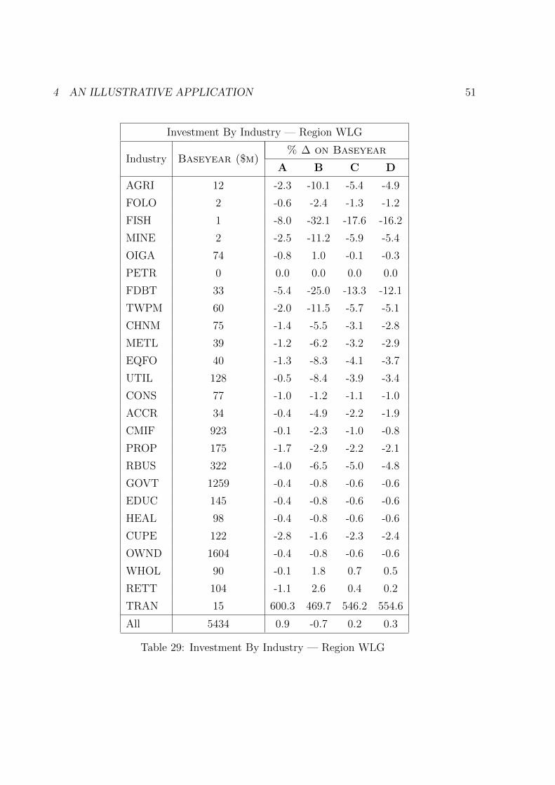
4 AN ILLUSTRATIVE APPLICATION 51
Investment By Industry — Region WLG
Industry Baseyear ($m)% ∆ on Baseyear
A B C D
AGRI 12 -2.3 -10.1 -5.4 -4.9
FOLO 2 -0.6 -2.4 -1.3 -1.2
FISH 1 -8.0 -32.1 -17.6 -16.2
MINE 2 -2.5 -11.2 -5.9 -5.4
OIGA 74 -0.8 1.0 -0.1 -0.3
PETR 0 0.0 0.0 0.0 0.0
FDBT 33 -5.4 -25.0 -13.3 -12.1
TWPM 60 -2.0 -11.5 -5.7 -5.1
CHNM 75 -1.4 -5.5 -3.1 -2.8
METL 39 -1.2 -6.2 -3.2 -2.9
EQFO 40 -1.3 -8.3 -4.1 -3.7
UTIL 128 -0.5 -8.4 -3.9 -3.4
CONS 77 -1.0 -1.2 -1.1 -1.0
ACCR 34 -0.4 -4.9 -2.2 -1.9
CMIF 923 -0.1 -2.3 -1.0 -0.8
PROP 175 -1.7 -2.9 -2.2 -2.1
RBUS 322 -4.0 -6.5 -5.0 -4.8
GOVT 1259 -0.4 -0.8 -0.6 -0.6
EDUC 145 -0.4 -0.8 -0.6 -0.6
HEAL 98 -0.4 -0.8 -0.6 -0.6
CUPE 122 -2.8 -1.6 -2.3 -2.4
OWND 1604 -0.4 -0.8 -0.6 -0.6
WHOL 90 -0.1 1.8 0.7 0.5
RETT 104 -1.1 2.6 0.4 0.2
TRAN 15 600.3 469.7 546.2 554.6
All 5434 0.9 -0.7 0.2 0.3
Table 29: Investment By Industry — Region WLG
5 CONCLUSION 52
5 Conclusion
By considering a set of scenarios concerning a natural disaster, we have seen the kind of
insights that may be obtained through the application of a multi-regional CGE model
to an economic impact analysis of such an event. The bottom-up regional modelling of
the implemented JENNIFER model not only allows for region-specific supply side shocks
as seen in our application, but also facilitates analysis of the impact of migration flows
in the wake of the disaster. Modelling household sensitivity to both relative regional
amenity and real wage rates helps build a detailed picture of inter-regional migration and
associated composition effects. With the JENNIFER model being prototype in nature,
there are a number of developments that would enable more useful results to be obtained
and improve the realism of the scenarios.
One development particularly relevant to supply-side shock scenarios would be a link
from the resources of the economy (and possibly quality-of-life measures) to regional
amenity along with an estimated functional relationship between changes in amenity and
household migration. This could potentially remove the need for running the no-mobility
intermediate simulation. Also useful for these scenarios and in general would be modelling
of local government including its relationship to central government, allowance for cross-
regional ownership of capital, and the regional distribution of employment by occupation.
These issues were not pursued due to time constraints. Analysis of the long-run effects of
our disaster scenario would be more complex, requiring a dynamic model of the economy
connected to a demographic growth model. Finally, the reliability of the scenario results
depends heavily on the quality of data used to drive the model. More work is required to
validate the assumed substitution elasticities and incorporate the available econometric
estimates of migration elasticities.

53
Appendices
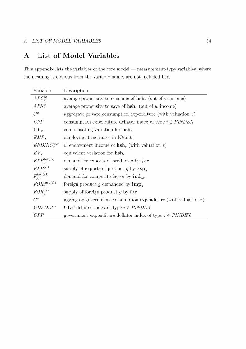
A LIST OF MODEL VARIABLES 54
A List of Model Variables
This appendix lists the variables of the core model — measurement-type variables, where
the meaning is obvious from the variable name, are not included here.
Variable Description
APCwr average propensity to consume of hshr (out of w income)
APSwr average propensity to save of hshr (out of w income)
Cv aggregate private consumption expenditure (with valuation v)
CPI i consumption expenditure deflator index of type i ∈ PINDEX
CV r compensating variation for hshr
EMP• employment measures in IOunits
ENDINCw,vr w endowment income of hshr (with valuation v)
EV r equivalent variation for hshr
EXP for(D)g demand for exports of product g by for
EXP (S)g supply of exports of product g by expg
Find(D)j,r demand for composite factor by indj,r
FORimp(D)g foreign product g demanded by impg
FOR(S)g supply of foreign product g by for
Gv aggregate government consumption expenditure (with valuation v)
GDPDEF i GDP deflator index of type i ∈ PINDEX
GPI i government expenditure deflator index of type i ∈ PINDEX
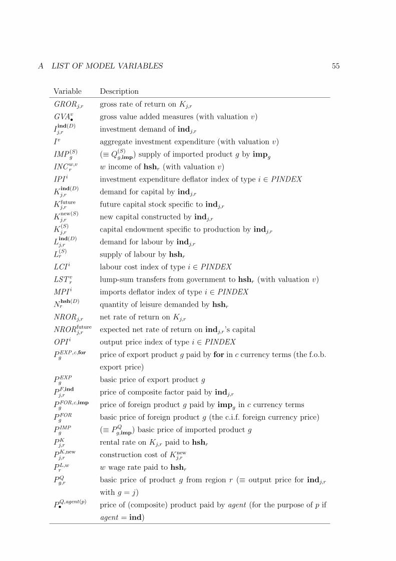
A LIST OF MODEL VARIABLES 55
Variable Description
GRORj,r gross rate of return on Kj,r
GVAv• gross value added measures (with valuation v)
Iind(D)j,r investment demand of indj,r
Iv aggregate investment expenditure (with valuation v)
IMP (S)g (≡ Q
(S)g,imp) supply of imported product g by impg
INCw,vr w income of hshr (with valuation v)
IPI i investment expenditure deflator index of type i ∈ PINDEX
Kind(D)j,r demand for capital by indj,r
K futurej,r future capital stock specific to indj,r
Knew(S)j,r new capital constructed by indj,r
K(S)j,r capital endowment specific to production by indj,r
Lind(D)j,r demand for labour by indj,r
L(S)r supply of labour by hshr
LCI i labour cost index of type i ∈ PINDEX
LST vr lump-sum transfers from government to hshr (with valuation v)
MPI i imports deflator index of type i ∈ PINDEX
Nhsh(D)r quantity of leisure demanded by hshr
NRORj,r net rate of return on Kj,r
NRORfuturej,r expected net rate of return on indj,r’s capital
OPI i output price index of type i ∈ PINDEX
PEXP ,c,forg price of export product g paid by for in c currency terms (the f.o.b.
export price)
PEXPg basic price of export product g
P F,indj,r price of composite factor paid by indj,r
PFOR,c,impg price of foreign product g paid by impg in c currency terms
PFORg basic price of foreign product g (the c.i.f. foreign currency price)
P IMPg (≡ PQ
g,imp) basic price of imported product g
PKj,r rental rate on Kj,r paid to hshr
PK,newj,r construction cost of Knew
j,r
PL,wr w wage rate paid to hshr
PQg,r basic price of product g from region r (≡ output price for indj,r
with g = j)
PQ,agent(p)• price of (composite) product paid by agent (for the purpose of p if
agent = ind)

A LIST OF MODEL VARIABLES 56
Variable Description
Qagent(p)(D)• (composite) product demanded by agent (for the purpose of p if
agent = ind)
Qagent(p)(D)• demand for undelivered (composite) product by agent (for the pur-
pose of p if agent = ind)
Q(S)g,r output (supply) of product g in region r (by indj,r with g = j)
Q(S)g,s supply of undelivered product g from source s
SAV w,vr w saving of hshr (with valuation v)
SPN vr expenditure of hshr (with valuation v)
TIME r time endowment of hshr
TPI i net trade deflator index of type i ∈ PINDEX
tEXPg export tax rate on product g (negative for subsidy)
tFORg import tariff rate on foreign product g
tGST ,agentg effective rate of GST faced by agent on product g
tQ,agent(p)• commodity tax rate faced by agent (for the purpose of p if agent =
ind)
tL average labour income tax rate
Ur utility of hshr
Wwr real w income wage rate
XPI i exports deflator index of type i ∈ PINDEX
δj,r depreciation rate on Kj,r
φ nominal exchange rate (domestic $ per foreign $)
ϕ real exchange rate
ψEXPg co-efficient reflecting the height of the export demand curve for
product g
Ω economy-wide average expected net rate of return on capital
Ξi Price index of type i ∈ PINDEX
RA/Bx Ratio of variable Ax to Bx
X•x,y/z Share of •x,y in •z (percent)
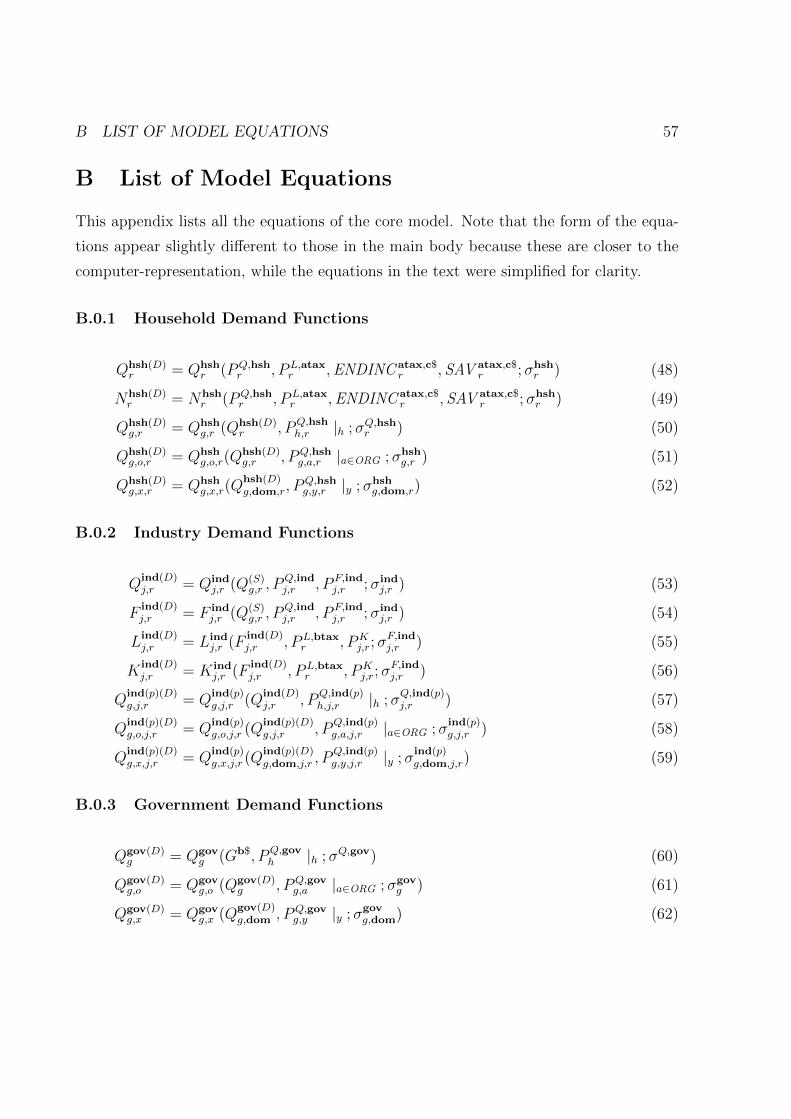
B LIST OF MODEL EQUATIONS 57
B List of Model Equations
This appendix lists all the equations of the core model. Note that the form of the equa-
tions appear slightly different to those in the main body because these are closer to the
computer-representation, while the equations in the text were simplified for clarity.
B.0.1 Household Demand Functions
Qhsh(D)r = Qhsh
r (PQ,hshr , PL,atax
r ,ENDINC atax,c$r , SAV atax,c$
r ;σhshr ) (48)
Nhsh(D)r = Nhsh
r (PQ,hshr , PL,atax
r ,ENDINC atax,c$r , SAV atax,c$
r ;σhshr ) (49)
Qhsh(D)g,r = Qhsh
g,r (Qhsh(D)r , PQ,hsh
h,r |h ;σQ,hshr ) (50)
Qhsh(D)g,o,r = Qhsh
g,o,r(Qhsh(D)g,r , PQ,hsh
g,a,r |a∈ORG ;σhshg,r ) (51)
Qhsh(D)g,x,r = Qhsh
g,x,r(Qhsh(D)g,dom,r, P
Q,hshg,y,r |y ;σhsh
g,dom,r) (52)
B.0.2 Industry Demand Functions
Qind(D)j,r = Qind
j,r (Q(S)g,r , P
Q,indj,r , P F,ind
j,r ;σindj,r ) (53)
Find(D)j,r = F ind
j,r (Q(S)g,r , P
Q,indj,r , P F,ind
j,r ;σindj,r ) (54)
Lind(D)j,r = Lind
j,r (Find(D)j,r , PL,btax
r , PKj,r;σ
F,indj,r ) (55)
Kind(D)j,r = K ind
j,r (Find(D)j,r , PL,btax
r , PKj,r;σ
F,indj,r ) (56)
Qind(p)(D)g,j,r = Q
ind(p)g,j,r (Q
ind(D)j,r , P
Q,ind(p)h,j,r |h ;σ
Q,ind(p)j,r ) (57)
Qind(p)(D)g,o,j,r = Q
ind(p)g,o,j,r (Q
ind(p)(D)g,j,r , P
Q,ind(p)g,a,j,r |a∈ORG ;σ
ind(p)g,j,r ) (58)
Qind(p)(D)g,x,j,r = Q
ind(p)g,x,j,r (Q
ind(p)(D)g,dom,j,r , P
Q,ind(p)g,y,j,r |y ;σ
ind(p)g,dom,j,r) (59)
B.0.3 Government Demand Functions
Qgov(D)g = Qgov
g (Gb$, PQ,govh |h ;σQ,gov) (60)
Qgov(D)g,o = Qgov
g,o (Qgov(D)g , PQ,gov
g,a |a∈ORG ;σgovg ) (61)
Qgov(D)g,x = Qgov
g,x (Qgov(D)g,dom , PQ,gov
g,y |y ;σgovg,dom) (62)
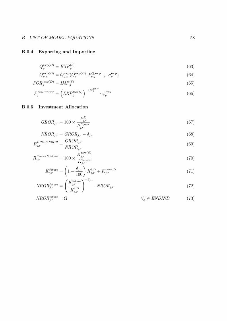
B LIST OF MODEL EQUATIONS 58
B.0.4 Exporting and Importing
Qexp(D)g = EXP (S)
g (63)
Qexp(D)g,x = Qexp
g,x (Qexp(D)g , PQ,exp
g,y |y ;σexpg ) (64)
FORimp(D)g = IMP (S)
g (65)
PEXP ,f$,forg =
(EXP for(D)
g
)−1/εEXPg
· ψEXPg (66)
B.0.5 Investment Allocation
GRORj,r = 100×PKj,r
PK,newj,r
(67)
NRORj,r = GRORj,r − δj,r (68)
RGROR/NRORj,r =
GRORj,r
NRORj,r
(69)
RKnew/Kfuturej,r = 100×
Knew(S)j,r
K futurej,r
(70)
K futurej,r =
(1− δj,r
100
)K
(S)j,r +K
new(S)j,r (71)
NRORfuturej,r =
(K futurej,r
K(S)j,r
)−βj,r· NRORj,r (72)
NRORfuturej,r = Ω ∀j ∈ ENDIND (73)
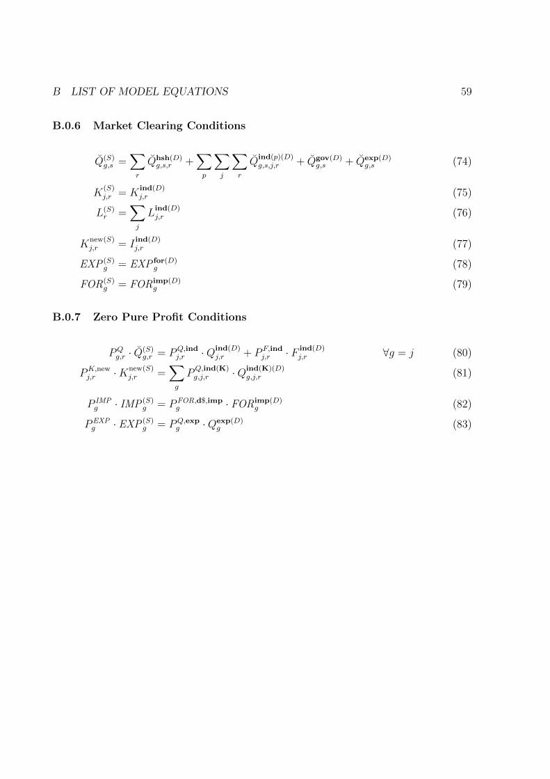
B LIST OF MODEL EQUATIONS 59
B.0.6 Market Clearing Conditions
Q(S)g,s =
∑r
Qhsh(D)g,s,r +
∑p
∑j
∑r
Qind(p)(D)g,s,j,r + Qgov(D)
g,s + Qexp(D)g,s (74)
K(S)j,r = K
ind(D)j,r (75)
L(S)r =
∑j
Lind(D)j,r (76)
Knew(S)j,r = I
ind(D)j,r (77)
EXP (S)g = EXP for(D)
g (78)
FOR(S)g = FORimp(D)
g (79)
B.0.7 Zero Pure Profit Conditions
PQg,r · Q(S)
g,r = PQ,indj,r ·Qind(D)
j,r + P F,indj,r · F ind(D)
j,r ∀g = j (80)
PK,newj,r ·Knew(S)
j,r =∑g
PQ,ind(K)g,j,r ·Qind(K)(D)
g,j,r (81)
P IMPg · IMP (S)
g = PFOR,d$,impg · FORimp(D)
g (82)
PEXPg · EXP (S)
g = PQ,expg ·Qexp(D)
g (83)
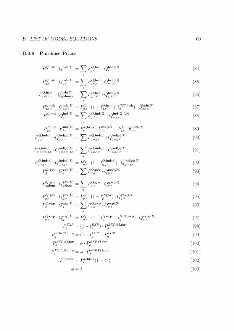
B LIST OF MODEL EQUATIONS 60
B.0.8 Purchase Prices
PQ,hshr ·Qhsh(D)
r =∑g
PQ,hshg,r ·Qhsh(D)
g,r (84)
PQ,hshg,r ·Qhsh(D)
g,r =∑o
PQ,hshg,o,r ·Qhsh(D)
g,o,r (85)
PQ,hshg,dom,r ·Q
hsh(D)g,dom,r =
∑x
PQ,hshg,x,r ·Qhsh(D)
g,x,r (86)
PQ,hshg,s,r ·Qhsh(D)
g,s,r = PQg,s · (1 + tQ,hshg,r + tGST ,hsh
g ) · Qhsh(D)g,s,r (87)
PQ,indj,r ·Qind(D)
j,r =∑g
PQ,ind(Q)g,j,r ·Qind(Q)(D)
g,j,r (88)
P F,indj,r · F ind(D)
j,r = PL,btaxr · Lind(D)
j,r + PKj,r ·K
ind(D)j,r (89)
PQ,ind(p)g,j,r ·Qind(p)(D)
g,j,r =∑o
PQ,ind(p)g,o,j,r ·Qind(p)(D)
g,o,j,r (90)
PQ,ind(p)g,dom,j,r ·Q
ind(p)(D)g,dom,j,r =
∑x
PQ,ind(p)g,x,j,r ·Qind(p)(D)
g,x,j,r (91)
PQ,ind(p)g,s,j,r ·Qind(p)(D)
g,s,j,r = PQg,s · (1 + t
Q,ind(p)g,j,r ) · Qind(p)(D)
g,s,j,r (92)
PQ,govg ·Qgov(D)
g =∑o
PQ,govg,o ·Qgov(D)
g,o (93)
PQ,govg,dom ·Q
gov(D)g,dom =
∑x
PQ,govg,x ·Qgov(D)
g,x (94)
PQ,govg,s ·Qgov(D)
g,s = PQg,s · (1 + tQ,govg ) · Qgov(D)
g,s (95)
PQ,expg ·Qexp(D)
g =∑x
PQ,expg,x ·Qexp(D)
g,x (96)
PQ,expg,x ·Qexp(D)
g,x = PQg,x · (1 + tQ,expg + tGST ,exp
g ) · Qexp(D)g,x (97)
PEXPg = (1− tEXP
g ) · PEXP ,d$,forg (98)
PFOR,f$,impg = (1 + tFOR
g ) · PFORg (99)
PEXP ,d$,forg = φ · PEXP ,f$,for
g (100)
PFOR,d$,impg = φ · PFOR,f$,imp
g (101)
PL,ataxr = PL,btax
r (1− tL) (102)
φ = 1 (103)
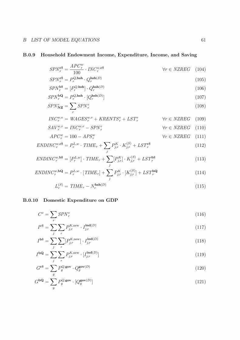
B LIST OF MODEL EQUATIONS 61
B.0.9 Household Endowment Income, Expenditure, Income, and Saving
SPN c$r =
APCwr
100· INCw,c$
r ∀r ∈ NZREG (104)
SPN c$r = PQ,hsh
r ·Qhsh(D)r (105)
SPN b$r = [PQ,hsh
r ] ·Qhsh(D)r (106)
SPN bQr = PQ,hsh
r · [Qhsh(D)r ] (107)
SPN vNZ =
∑r
SPN vr (108)
INCw,vr = WAGESw,vr + KRENTS vr + LST v
r ∀r ∈ NZREG (109)
SAV w,vr = INCw,v
r − SPN vr ∀r ∈ NZREG (110)
APCwr = 100− APSwr ∀r ∈ NZREG (111)
ENDINCw,c$r = PL,w
r · TIME r +∑j
PKj,r ·K
(S)j,r + LST c$
r (112)
ENDINCw,b$r = [PL,w
r ] · TIME r +∑j
[PKj,r] ·K
(S)j,r + LSTb$
r (113)
ENDINCw,bQr = PL,w
r · [TIME r] +∑j
PKj,r · [K
(S)j,r ] + LSTbQ
r (114)
L(S)r = TIME r −Nhsh(D)
r (115)
B.0.10 Domestic Expenditure on GDP
Cv =∑r
SPN vr (116)
Ic$ =∑j
∑r
PK,newj,r · I ind(D)
j,r (117)
Ib$ =∑j
∑r
[PK,newj,r ] · I ind(D)
j,r (118)
IbQ =∑j
∑r
PK,newj,r · [I ind(D)
j,r ] (119)
Gc$ =∑g
PQ,govg ·Qgov(D)
g (120)
GbQ =∑g
PQ,govg · [Qgov(D)
g ] (121)
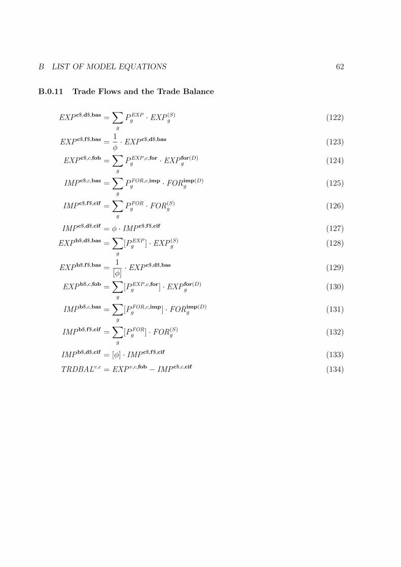
B LIST OF MODEL EQUATIONS 62
B.0.11 Trade Flows and the Trade Balance
EXPc$,d$,bas =∑g
PEXPg · EXP (S)
g (122)
EXPc$,f$,bas =1
φ· EXPc$,d$,bas (123)
EXPc$,c,fob =∑g
PEXP ,c,forg · EXP for(D)
g (124)
IMPc$,c,bas =∑g
PFOR,c,impg · FORimp(D)
g (125)
IMPc$,f$,cif =∑g
PFORg · FOR(S)
g (126)
IMPc$,d$,cif = φ · IMPc$,f$,cif (127)
EXPb$,d$,bas =∑g
[PEXPg ] · EXP (S)
g (128)
EXPb$,f$,bas =1
[φ]· EXPc$,d$,bas (129)
EXPb$,c,fob =∑g
[PEXP ,c,forg ] · EXP for(D)
g (130)
IMPb$,c,bas =∑g
[PFOR,c,impg ] · FORimp(D)
g (131)
IMPb$,f$,cif =∑g
[PFORg ] · FOR(S)
g (132)
IMPb$,d$,cif = [φ] · IMPc$,f$,cif (133)
TRDBALv,c = EXPv,c,fob − IMPc$,c,cif (134)
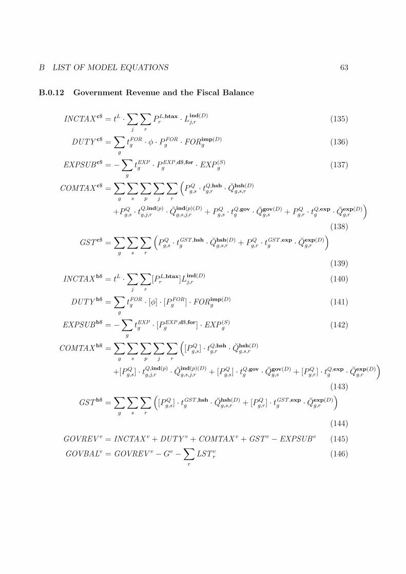
B LIST OF MODEL EQUATIONS 63
B.0.12 Government Revenue and the Fiscal Balance
INCTAX c$ = tL ·∑j
∑r
PL,btaxr · Lind(D)
j,r (135)
DUTY c$ =∑g
tFORg · φ · PFOR
g · FORimp(D)g (136)
EXPSUBc$ = −∑g
tEXPg · PEXP ,d$,for
g · EXP (S)g (137)
COMTAX c$ =∑g
∑s
∑p
∑j
∑r
(PQg,s · tQ,hshg,r · Qhsh(D)
g,s,r
+PQg,s · t
Q,ind(p)g,j,r · Qind(p)(D)
g,s,j,r + PQg,s · tQ,govg · Qgov(D)
g,s + PQg,r · tQ,expg · Qexp(D)
g,r
)(138)
GST c$ =∑g
∑s
∑r
(PQg,s · tGST ,hsh
g · Qhsh(D)g,s,r + PQ
g,r · tGST ,expg · Qexp(D)
g,r
)(139)
INCTAX b$ = tL ·∑j
∑r
[PL,btaxr ]L
ind(D)j,r (140)
DUTY b$ =∑g
tFORg · [φ] · [PFOR
g ] · FORimp(D)g (141)
EXPSUBb$ = −∑g
tEXPg · [PEXP ,d$,for
g ] · EXP (S)g (142)
COMTAX b$ =∑g
∑s
∑p
∑j
∑r
([PQg,s] · tQ,hshg,r · Qhsh(D)
g,s,r
+[PQg,s] · t
Q,ind(p)g,j,r · Qind(p)(D)
g,s,j,r + [PQg,s] · tQ,govg · Qgov(D)
g,s + [PQg,r] · tQ,expg · Qexp(D)
g,r
)(143)
GSTb$ =∑g
∑s
∑r
([PQg,s] · tGST ,hsh
g · Qhsh(D)g,s,r + [PQ
g,r] · tGST ,expg · Qexp(D)
g,r
)(144)
GOVREV v = INCTAX v + DUTY v + COMTAX v + GST v − EXPSUBv (145)
GOVBALv = GOVREV v −Gv −∑r
LST vr (146)
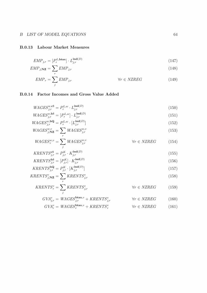
B LIST OF MODEL EQUATIONS 64
B.0.13 Labour Market Measures
EMP j,r = [PL,btaxr ] · Lind(D)
j,r (147)
EMP j,NZ =∑r
EMP j,r (148)
EMP r =∑j
EMP j,r ∀r ∈ NZREG (149)
B.0.14 Factor Incomes and Gross Value Added
WAGESw,c$j,r = PL,w
r · Lind(D)j,r (150)
WAGESw,b$j,r = [PL,w
r ] · Lind(D)j,r (151)
WAGESw,bQj,r = PL,wr · [Lind(D)
j,r ] (152)
WAGESw,vj,NZ =∑r
WAGESw,vj,r (153)
WAGESw,vr =∑j
WAGESw,vj,r ∀r ∈ NZREG (154)
KRENTS c$j,r = PK
j,r ·Kind(D)j,r (155)
KRENTSb$j,r = [PK
j,r] ·Kind(D)j,r (156)
KRENTSbQj,r = PK
j,r · [Kind(D)j,r ] (157)
KRENTS vj,NZ =∑r
KRENTS vj,r (158)
KRENTS vr =∑j
KRENTS vj,r ∀r ∈ NZREG (159)
GVAvj,r = WAGESbtax,v
j,r + KRENTS vj,r ∀r ∈ NZREG (160)
GVAvr = WAGESbtax,v
r + KRENTS vr ∀r ∈ NZREG (161)
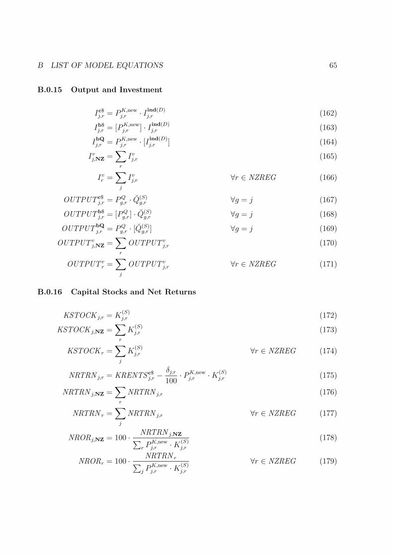
B LIST OF MODEL EQUATIONS 65
B.0.15 Output and Investment
Ic$j,r = PK,new
j,r · I ind(D)j,r (162)
Ib$j,r = [PK,new
j,r ] · I ind(D)j,r (163)
IbQj,r = PK,newj,r · [I ind(D)
j,r ] (164)
Ivj,NZ =∑r
Ivj,r (165)
Ivr =∑j
Ivj,r ∀r ∈ NZREG (166)
OUTPUT c$j,r = PQ
g,r · Q(S)g,r ∀g = j (167)
OUTPUTb$j,r = [PQ
g,r] · Q(S)g,r ∀g = j (168)
OUTPUTbQj,r = PQ
g,r · [Q(S)g,r ] ∀g = j (169)
OUTPUT vj,NZ =
∑r
OUTPUT vj,r (170)
OUTPUT vr =
∑j
OUTPUT vj,r ∀r ∈ NZREG (171)
B.0.16 Capital Stocks and Net Returns
KSTOCK j,r = K(S)j,r (172)
KSTOCK j,NZ =∑r
K(S)j,r (173)
KSTOCK r =∑j
K(S)j,r ∀r ∈ NZREG (174)
NRTRN j,r = KRENTS c$j,r −
δj,r100· PK,new
j,r ·K(S)j,r (175)
NRTRN j,NZ =∑r
NRTRN j,r (176)
NRTRN r =∑j
NRTRN j,r ∀r ∈ NZREG (177)
NRORj,NZ = 100 · NRTRN j,NZ∑r P
K,newj,r ·K(S)
j,r
(178)
NRORr = 100 · NRTRN r∑j P
K,newj,r ·K(S)
j,r
∀r ∈ NZREG (179)
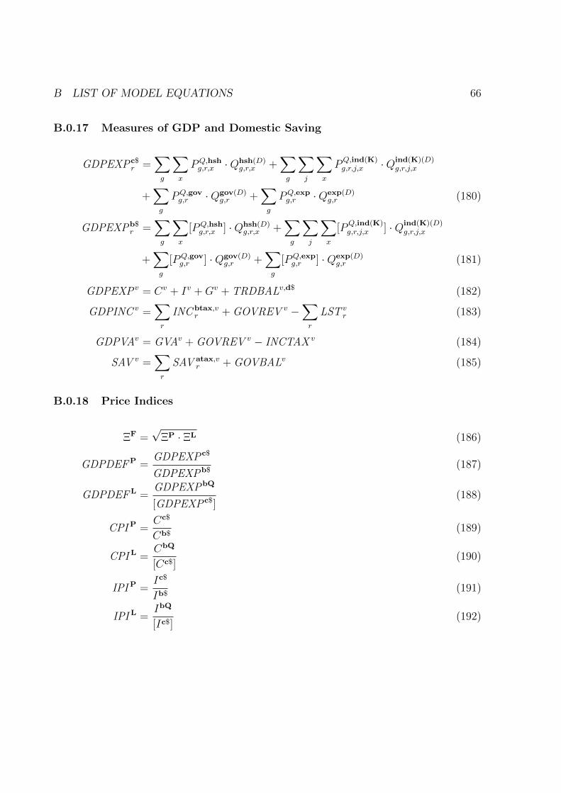
B LIST OF MODEL EQUATIONS 66
B.0.17 Measures of GDP and Domestic Saving
GDPEXPc$r =
∑g
∑x
PQ,hshg,r,x ·Qhsh(D)
g,r,x +∑g
∑j
∑x
PQ,ind(K)g,r,j,x ·Qind(K)(D)
g,r,j,x
+∑g
PQ,govg,r ·Qgov(D)
g,r +∑g
PQ,expg,r ·Qexp(D)
g,r (180)
GDPEXPb$r =
∑g
∑x
[PQ,hshg,r,x ] ·Qhsh(D)
g,r,x +∑g
∑j
∑x
[PQ,ind(K)g,r,j,x ] ·Qind(K)(D)
g,r,j,x
+∑g
[PQ,govg,r ] ·Qgov(D)
g,r +∑g
[PQ,expg,r ] ·Qexp(D)
g,r (181)
GDPEXPv = Cv + Iv +Gv + TRDBALv,d$ (182)
GDPINC v =∑r
INC btax,vr + GOVREV v −
∑r
LST vr (183)
GDPVAv = GVAv + GOVREV v − INCTAX v (184)
SAV v =∑r
SAV atax,vr + GOVBALv (185)
B.0.18 Price Indices
ΞF =√
ΞP · ΞL (186)
GDPDEFP =GDPEXPc$
GDPEXPb$(187)
GDPDEFL =GDPEXPbQ
[GDPEXPc$](188)
CPIP =Cc$
Cb$(189)
CPI L =CbQ
[Cc$](190)
IPIP =Ic$
Ib$(191)
IPI L =IbQ
[Ic$](192)
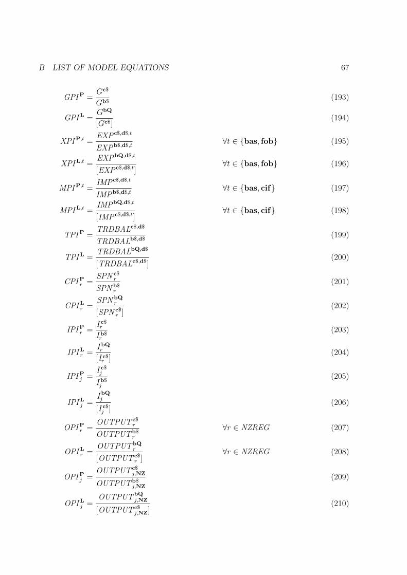
B LIST OF MODEL EQUATIONS 67
GPIP =Gc$
Gb$(193)
GPI L =GbQ
[Gc$](194)
XPIP,t =EXPc$,d$,t
EXPb$,d$,t∀t ∈ bas, fob (195)
XPI L,t =EXPbQ,d$,t
[EXPc$,d$,t]∀t ∈ bas, fob (196)
MPIP,t =IMPc$,d$,t
IMPb$,d$,t∀t ∈ bas, cif (197)
MPI L,t =IMPbQ,d$,t
[IMPc$,d$,t]∀t ∈ bas, cif (198)
TPIP =TRDBALc$,d$
TRDBALb$,d$(199)
TPI L =TRDBALbQ,d$
[TRDBALc$,d$](200)
CPIPr =SPN c$
r
SPN b$r
(201)
CPI Lr =SPN bQ
r
[SPN c$r ]
(202)
IPIPr =I c$r
I b$r
(203)
IPI Lr =I bQr[I c$r ]
(204)
IPIPj =I c$j
I b$j
(205)
IPI Lj =I bQj
[I c$j ]
(206)
OPIPr =OUTPUT c$
r
OUTPUTb$r
∀r ∈ NZREG (207)
OPI Lr =OUTPUTbQ
r
[OUTPUT c$r ]
∀r ∈ NZREG (208)
OPIPj =OUTPUT c$
j,NZ
OUTPUTb$j,NZ
(209)
OPI Lj =OUTPUTbQ
j,NZ
[OUTPUT c$j,NZ]
(210)
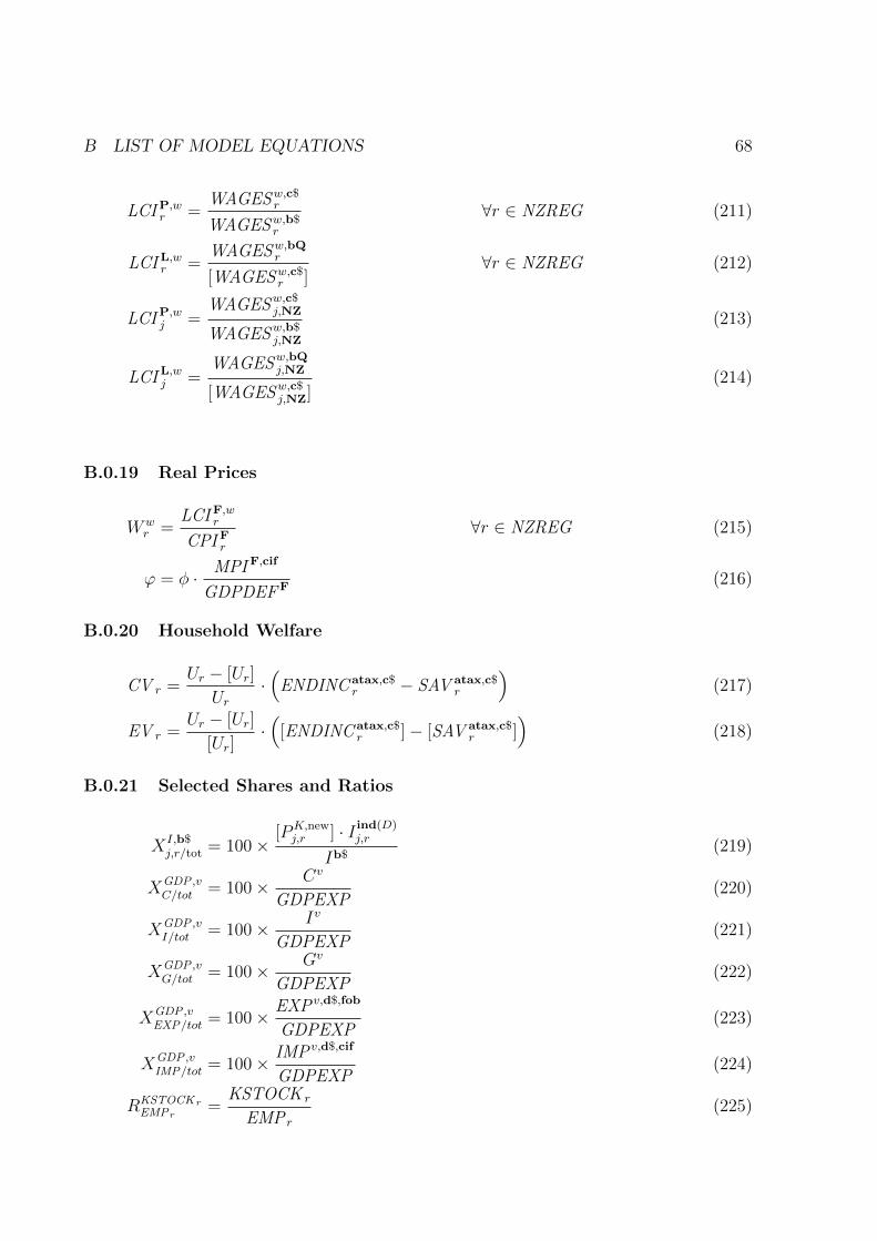
B LIST OF MODEL EQUATIONS 68
LCIP,wr =WAGESw,c$
r
WAGESw,b$r
∀r ∈ NZREG (211)
LCI L,wr =WAGESw,bQr
[WAGESw,c$r ]
∀r ∈ NZREG (212)
LCIP,wj =WAGESw,c$
j,NZ
WAGESw,b$j,NZ
(213)
LCI L,wj =WAGESw,bQj,NZ
[WAGESw,c$j,NZ]
(214)
B.0.19 Real Prices
Wwr =
LCI F,wr
CPI Fr∀r ∈ NZREG (215)
ϕ = φ · MPI F,cif
GDPDEFF(216)
B.0.20 Household Welfare
CV r =Ur − [Ur]
Ur·(ENDINC atax,c$
r − SAV atax,c$r
)(217)
EV r =Ur − [Ur]
[Ur]·(
[ENDINC atax,c$r ]− [SAV atax,c$
r ])
(218)
B.0.21 Selected Shares and Ratios
XI,b$j,r/tot = 100×
[PK,newj,r ] · I ind(D)
j,r
Ib$(219)
XGDP ,vC/tot = 100× Cv
GDPEXP(220)
XGDP ,vI/tot = 100× Iv
GDPEXP(221)
XGDP ,vG/tot = 100× Gv
GDPEXP(222)
XGDP ,vEXP/tot = 100× EXPv,d$,fob
GDPEXP(223)
XGDP ,vIMP/tot = 100× IMPv,d$,cif
GDPEXP(224)
RKSTOCK rEMPr
=KSTOCK r
EMP r
(225)

C ADDITIONAL RESULTS 69
C Additional Results
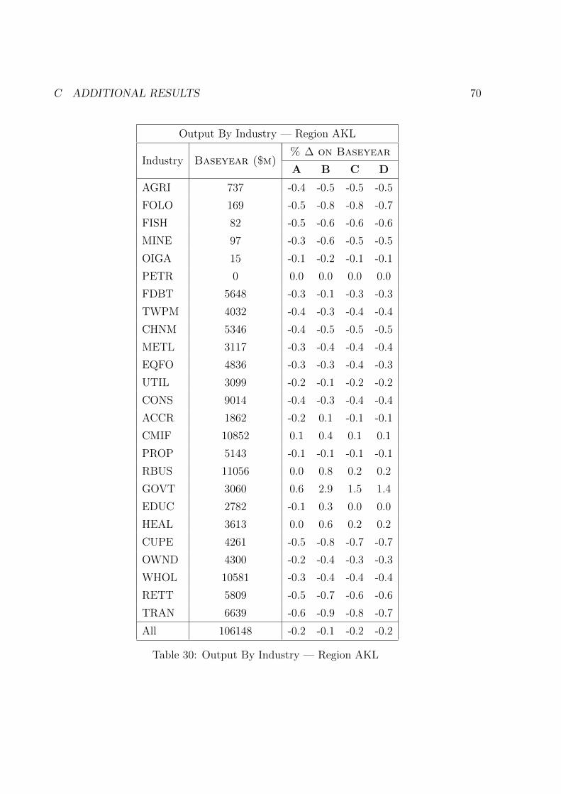
C ADDITIONAL RESULTS 70
Output By Industry — Region AKL
Industry Baseyear ($m)% ∆ on Baseyear
A B C D
AGRI 737 -0.4 -0.5 -0.5 -0.5
FOLO 169 -0.5 -0.8 -0.8 -0.7
FISH 82 -0.5 -0.6 -0.6 -0.6
MINE 97 -0.3 -0.6 -0.5 -0.5
OIGA 15 -0.1 -0.2 -0.1 -0.1
PETR 0 0.0 0.0 0.0 0.0
FDBT 5648 -0.3 -0.1 -0.3 -0.3
TWPM 4032 -0.4 -0.3 -0.4 -0.4
CHNM 5346 -0.4 -0.5 -0.5 -0.5
METL 3117 -0.3 -0.4 -0.4 -0.4
EQFO 4836 -0.3 -0.3 -0.4 -0.3
UTIL 3099 -0.2 -0.1 -0.2 -0.2
CONS 9014 -0.4 -0.3 -0.4 -0.4
ACCR 1862 -0.2 0.1 -0.1 -0.1
CMIF 10852 0.1 0.4 0.1 0.1
PROP 5143 -0.1 -0.1 -0.1 -0.1
RBUS 11056 0.0 0.8 0.2 0.2
GOVT 3060 0.6 2.9 1.5 1.4
EDUC 2782 -0.1 0.3 0.0 0.0
HEAL 3613 0.0 0.6 0.2 0.2
CUPE 4261 -0.5 -0.8 -0.7 -0.7
OWND 4300 -0.2 -0.4 -0.3 -0.3
WHOL 10581 -0.3 -0.4 -0.4 -0.4
RETT 5809 -0.5 -0.7 -0.6 -0.6
TRAN 6639 -0.6 -0.9 -0.8 -0.7
All 106148 -0.2 -0.1 -0.2 -0.2
Table 30: Output By Industry — Region AKL
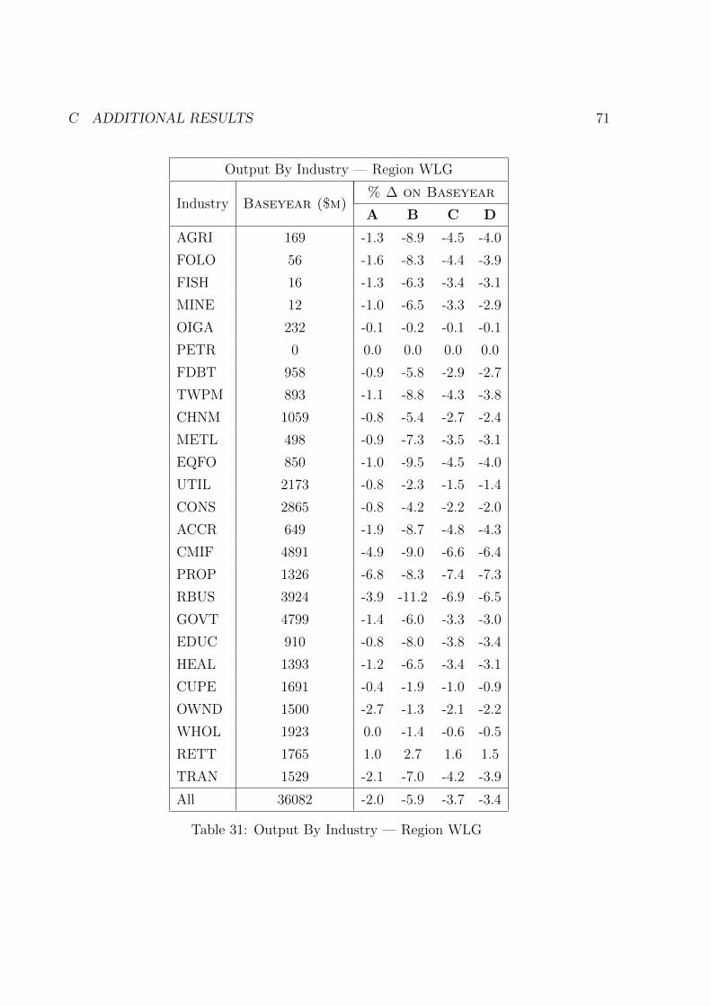
C ADDITIONAL RESULTS 71
Output By Industry — Region WLG
Industry Baseyear ($m)% ∆ on Baseyear
A B C D
AGRI 169 -1.3 -8.9 -4.5 -4.0
FOLO 56 -1.6 -8.3 -4.4 -3.9
FISH 16 -1.3 -6.3 -3.4 -3.1
MINE 12 -1.0 -6.5 -3.3 -2.9
OIGA 232 -0.1 -0.2 -0.1 -0.1
PETR 0 0.0 0.0 0.0 0.0
FDBT 958 -0.9 -5.8 -2.9 -2.7
TWPM 893 -1.1 -8.8 -4.3 -3.8
CHNM 1059 -0.8 -5.4 -2.7 -2.4
METL 498 -0.9 -7.3 -3.5 -3.1
EQFO 850 -1.0 -9.5 -4.5 -4.0
UTIL 2173 -0.8 -2.3 -1.5 -1.4
CONS 2865 -0.8 -4.2 -2.2 -2.0
ACCR 649 -1.9 -8.7 -4.8 -4.3
CMIF 4891 -4.9 -9.0 -6.6 -6.4
PROP 1326 -6.8 -8.3 -7.4 -7.3
RBUS 3924 -3.9 -11.2 -6.9 -6.5
GOVT 4799 -1.4 -6.0 -3.3 -3.0
EDUC 910 -0.8 -8.0 -3.8 -3.4
HEAL 1393 -1.2 -6.5 -3.4 -3.1
CUPE 1691 -0.4 -1.9 -1.0 -0.9
OWND 1500 -2.7 -1.3 -2.1 -2.2
WHOL 1923 0.0 -1.4 -0.6 -0.5
RETT 1765 1.0 2.7 1.6 1.5
TRAN 1529 -2.1 -7.0 -4.2 -3.9
All 36082 -2.0 -5.9 -3.7 -3.4
Table 31: Output By Industry — Region WLG
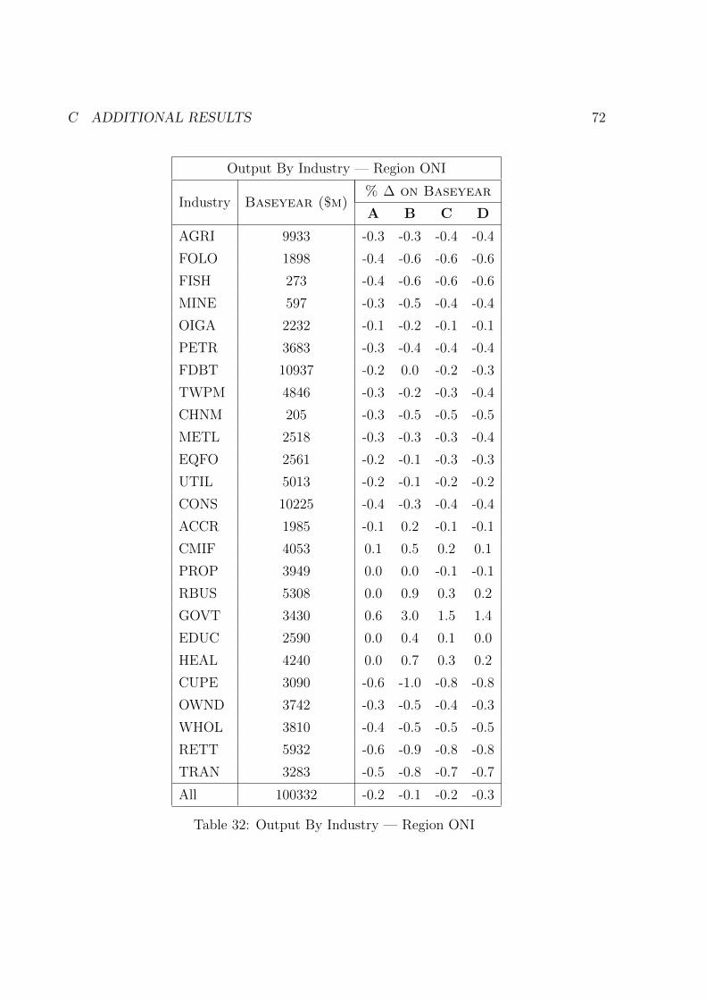
C ADDITIONAL RESULTS 72
Output By Industry — Region ONI
Industry Baseyear ($m)% ∆ on Baseyear
A B C D
AGRI 9933 -0.3 -0.3 -0.4 -0.4
FOLO 1898 -0.4 -0.6 -0.6 -0.6
FISH 273 -0.4 -0.6 -0.6 -0.6
MINE 597 -0.3 -0.5 -0.4 -0.4
OIGA 2232 -0.1 -0.2 -0.1 -0.1
PETR 3683 -0.3 -0.4 -0.4 -0.4
FDBT 10937 -0.2 0.0 -0.2 -0.3
TWPM 4846 -0.3 -0.2 -0.3 -0.4
CHNM 205 -0.3 -0.5 -0.5 -0.5
METL 2518 -0.3 -0.3 -0.3 -0.4
EQFO 2561 -0.2 -0.1 -0.3 -0.3
UTIL 5013 -0.2 -0.1 -0.2 -0.2
CONS 10225 -0.4 -0.3 -0.4 -0.4
ACCR 1985 -0.1 0.2 -0.1 -0.1
CMIF 4053 0.1 0.5 0.2 0.1
PROP 3949 0.0 0.0 -0.1 -0.1
RBUS 5308 0.0 0.9 0.3 0.2
GOVT 3430 0.6 3.0 1.5 1.4
EDUC 2590 0.0 0.4 0.1 0.0
HEAL 4240 0.0 0.7 0.3 0.2
CUPE 3090 -0.6 -1.0 -0.8 -0.8
OWND 3742 -0.3 -0.5 -0.4 -0.3
WHOL 3810 -0.4 -0.5 -0.5 -0.5
RETT 5932 -0.6 -0.9 -0.8 -0.8
TRAN 3283 -0.5 -0.8 -0.7 -0.7
All 100332 -0.2 -0.1 -0.2 -0.3
Table 32: Output By Industry — Region ONI
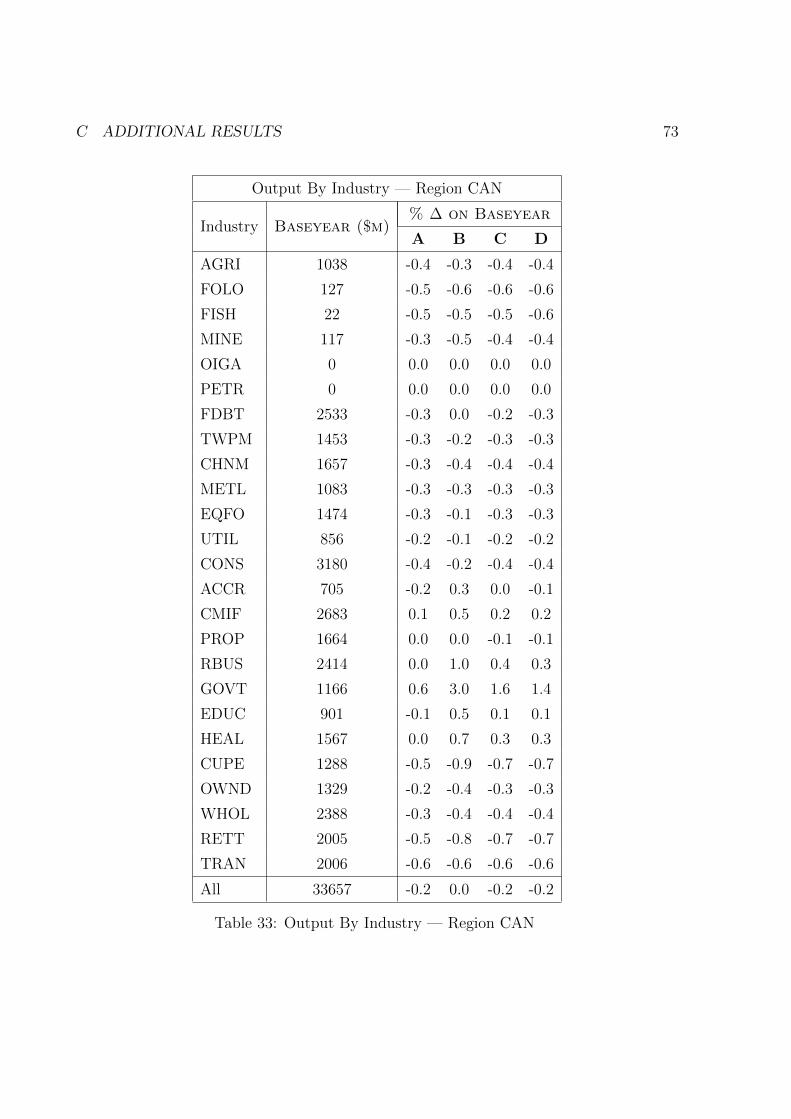
C ADDITIONAL RESULTS 73
Output By Industry — Region CAN
Industry Baseyear ($m)% ∆ on Baseyear
A B C D
AGRI 1038 -0.4 -0.3 -0.4 -0.4
FOLO 127 -0.5 -0.6 -0.6 -0.6
FISH 22 -0.5 -0.5 -0.5 -0.6
MINE 117 -0.3 -0.5 -0.4 -0.4
OIGA 0 0.0 0.0 0.0 0.0
PETR 0 0.0 0.0 0.0 0.0
FDBT 2533 -0.3 0.0 -0.2 -0.3
TWPM 1453 -0.3 -0.2 -0.3 -0.3
CHNM 1657 -0.3 -0.4 -0.4 -0.4
METL 1083 -0.3 -0.3 -0.3 -0.3
EQFO 1474 -0.3 -0.1 -0.3 -0.3
UTIL 856 -0.2 -0.1 -0.2 -0.2
CONS 3180 -0.4 -0.2 -0.4 -0.4
ACCR 705 -0.2 0.3 0.0 -0.1
CMIF 2683 0.1 0.5 0.2 0.2
PROP 1664 0.0 0.0 -0.1 -0.1
RBUS 2414 0.0 1.0 0.4 0.3
GOVT 1166 0.6 3.0 1.6 1.4
EDUC 901 -0.1 0.5 0.1 0.1
HEAL 1567 0.0 0.7 0.3 0.3
CUPE 1288 -0.5 -0.9 -0.7 -0.7
OWND 1329 -0.2 -0.4 -0.3 -0.3
WHOL 2388 -0.3 -0.4 -0.4 -0.4
RETT 2005 -0.5 -0.8 -0.7 -0.7
TRAN 2006 -0.6 -0.6 -0.6 -0.6
All 33657 -0.2 0.0 -0.2 -0.2
Table 33: Output By Industry — Region CAN
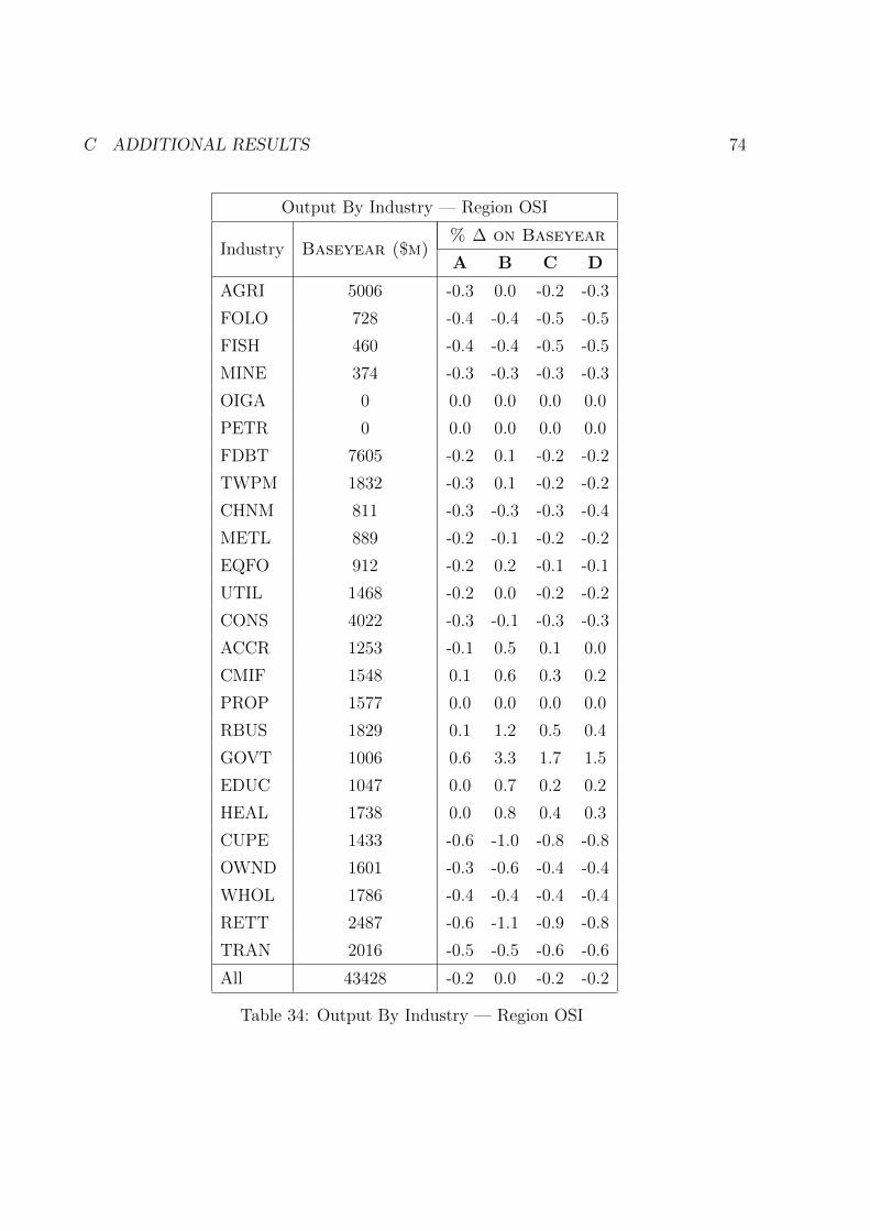
C ADDITIONAL RESULTS 74
Output By Industry — Region OSI
Industry Baseyear ($m)% ∆ on Baseyear
A B C D
AGRI 5006 -0.3 0.0 -0.2 -0.3
FOLO 728 -0.4 -0.4 -0.5 -0.5
FISH 460 -0.4 -0.4 -0.5 -0.5
MINE 374 -0.3 -0.3 -0.3 -0.3
OIGA 0 0.0 0.0 0.0 0.0
PETR 0 0.0 0.0 0.0 0.0
FDBT 7605 -0.2 0.1 -0.2 -0.2
TWPM 1832 -0.3 0.1 -0.2 -0.2
CHNM 811 -0.3 -0.3 -0.3 -0.4
METL 889 -0.2 -0.1 -0.2 -0.2
EQFO 912 -0.2 0.2 -0.1 -0.1
UTIL 1468 -0.2 0.0 -0.2 -0.2
CONS 4022 -0.3 -0.1 -0.3 -0.3
ACCR 1253 -0.1 0.5 0.1 0.0
CMIF 1548 0.1 0.6 0.3 0.2
PROP 1577 0.0 0.0 0.0 0.0
RBUS 1829 0.1 1.2 0.5 0.4
GOVT 1006 0.6 3.3 1.7 1.5
EDUC 1047 0.0 0.7 0.2 0.2
HEAL 1738 0.0 0.8 0.4 0.3
CUPE 1433 -0.6 -1.0 -0.8 -0.8
OWND 1601 -0.3 -0.6 -0.4 -0.4
WHOL 1786 -0.4 -0.4 -0.4 -0.4
RETT 2487 -0.6 -1.1 -0.9 -0.8
TRAN 2016 -0.5 -0.5 -0.6 -0.6
All 43428 -0.2 0.0 -0.2 -0.2
Table 34: Output By Industry — Region OSI

C ADDITIONAL RESULTS 75
Employment By Industry — Region AKL (FTEs)
Industry Baseyear (000s)% ∆ on Baseyear
A B C D
AGRI 8 -0.3 0.4 -0.2 -0.2
FOLO 0 -0.4 0.2 -0.4 -0.3
FISH 0 -0.3 0.5 -0.2 -0.1
MINE 0 -0.3 0.3 -0.2 -0.2
OIGA 0 0.0 0.0 0.0 0.0
PETR 0 0.0 0.0 0.0 0.0
FDBT 12 -0.2 0.8 0.0 0.0
TWPM 23 -0.2 0.6 -0.1 0.0
CHNM 10 -0.2 0.4 -0.1 -0.1
METL 10 -0.2 0.5 -0.1 -0.1
EQFO 19 -0.2 0.6 -0.1 0.0
UTIL 2 -0.1 1.4 0.3 0.3
CONS 43 -0.3 0.7 0.0 0.0
ACCR 25 0.0 1.0 0.2 0.2
CMIF 38 0.7 2.4 1.2 1.2
PROP 17 0.4 1.4 0.6 0.7
RBUS 81 0.3 2.1 0.9 0.8
GOVT 19 0.9 4.2 2.1 2.0
EDUC 38 0.0 0.9 0.3 0.3
HEAL 47 0.2 1.4 0.6 0.6
CUPE 25 -0.3 0.1 -0.3 -0.2
OWND 0 0.0 0.0 0.0 0.0
WHOL 43 -0.1 0.7 0.1 0.1
RETT 49 -0.3 0.1 -0.3 -0.3
TRAN 22 -0.3 0.3 -0.3 -0.2
All 533 0.1 1.2 0.4 0.4
Table 35: Employment By Industry — Region AKL
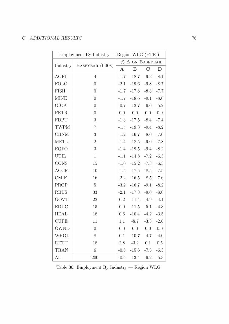
C ADDITIONAL RESULTS 76
Employment By Industry — Region WLG (FTEs)
Industry Baseyear (000s)% ∆ on Baseyear
A B C D
AGRI 4 -1.7 -18.7 -9.2 -8.1
FOLO 0 -2.1 -19.6 -9.8 -8.7
FISH 0 -1.7 -17.8 -8.8 -7.7
MINE 0 -1.7 -18.6 -9.1 -8.0
OIGA 0 -0.7 -12.7 -6.0 -5.2
PETR 0 0.0 0.0 0.0 0.0
FDBT 3 -1.3 -17.5 -8.4 -7.4
TWPM 7 -1.5 -19.3 -9.4 -8.2
CHNM 3 -1.2 -16.7 -8.0 -7.0
METL 2 -1.4 -18.5 -9.0 -7.8
EQFO 3 -1.4 -19.5 -9.4 -8.2
UTIL 1 -1.1 -14.8 -7.2 -6.3
CONS 15 -1.0 -15.2 -7.3 -6.3
ACCR 10 -1.5 -17.5 -8.5 -7.5
CMIF 16 -2.2 -16.5 -8.5 -7.6
PROP 5 -3.2 -16.7 -9.1 -8.2
RBUS 33 -2.1 -17.8 -9.0 -8.0
GOVT 22 0.2 -11.4 -4.9 -4.1
EDUC 15 0.0 -11.5 -5.1 -4.3
HEAL 18 0.6 -10.4 -4.2 -3.5
CUPE 11 1.1 -8.7 -3.3 -2.6
OWND 0 0.0 0.0 0.0 0.0
WHOL 8 0.1 -10.7 -4.7 -4.0
RETT 18 2.8 -3.2 0.1 0.5
TRAN 6 -0.8 -15.6 -7.3 -6.3
All 200 -0.5 -13.4 -6.2 -5.3
Table 36: Employment By Industry — Region WLG
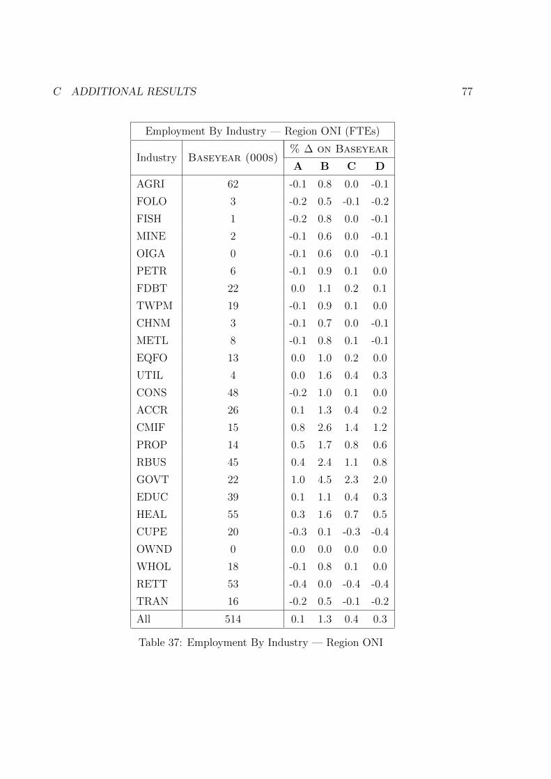
C ADDITIONAL RESULTS 77
Employment By Industry — Region ONI (FTEs)
Industry Baseyear (000s)% ∆ on Baseyear
A B C D
AGRI 62 -0.1 0.8 0.0 -0.1
FOLO 3 -0.2 0.5 -0.1 -0.2
FISH 1 -0.2 0.8 0.0 -0.1
MINE 2 -0.1 0.6 0.0 -0.1
OIGA 0 -0.1 0.6 0.0 -0.1
PETR 6 -0.1 0.9 0.1 0.0
FDBT 22 0.0 1.1 0.2 0.1
TWPM 19 -0.1 0.9 0.1 0.0
CHNM 3 -0.1 0.7 0.0 -0.1
METL 8 -0.1 0.8 0.1 -0.1
EQFO 13 0.0 1.0 0.2 0.0
UTIL 4 0.0 1.6 0.4 0.3
CONS 48 -0.2 1.0 0.1 0.0
ACCR 26 0.1 1.3 0.4 0.2
CMIF 15 0.8 2.6 1.4 1.2
PROP 14 0.5 1.7 0.8 0.6
RBUS 45 0.4 2.4 1.1 0.8
GOVT 22 1.0 4.5 2.3 2.0
EDUC 39 0.1 1.1 0.4 0.3
HEAL 55 0.3 1.6 0.7 0.5
CUPE 20 -0.3 0.1 -0.3 -0.4
OWND 0 0.0 0.0 0.0 0.0
WHOL 18 -0.1 0.8 0.1 0.0
RETT 53 -0.4 0.0 -0.4 -0.4
TRAN 16 -0.2 0.5 -0.1 -0.2
All 514 0.1 1.3 0.4 0.3
Table 37: Employment By Industry — Region ONI
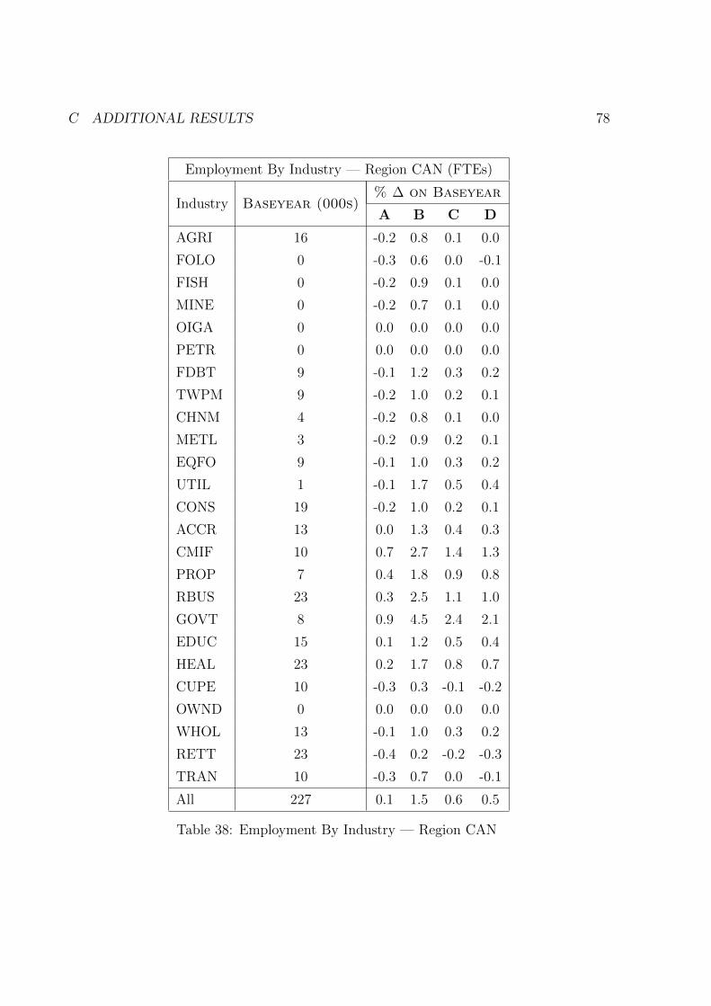
C ADDITIONAL RESULTS 78
Employment By Industry — Region CAN (FTEs)
Industry Baseyear (000s)% ∆ on Baseyear
A B C D
AGRI 16 -0.2 0.8 0.1 0.0
FOLO 0 -0.3 0.6 0.0 -0.1
FISH 0 -0.2 0.9 0.1 0.0
MINE 0 -0.2 0.7 0.1 0.0
OIGA 0 0.0 0.0 0.0 0.0
PETR 0 0.0 0.0 0.0 0.0
FDBT 9 -0.1 1.2 0.3 0.2
TWPM 9 -0.2 1.0 0.2 0.1
CHNM 4 -0.2 0.8 0.1 0.0
METL 3 -0.2 0.9 0.2 0.1
EQFO 9 -0.1 1.0 0.3 0.2
UTIL 1 -0.1 1.7 0.5 0.4
CONS 19 -0.2 1.0 0.2 0.1
ACCR 13 0.0 1.3 0.4 0.3
CMIF 10 0.7 2.7 1.4 1.3
PROP 7 0.4 1.8 0.9 0.8
RBUS 23 0.3 2.5 1.1 1.0
GOVT 8 0.9 4.5 2.4 2.1
EDUC 15 0.1 1.2 0.5 0.4
HEAL 23 0.2 1.7 0.8 0.7
CUPE 10 -0.3 0.3 -0.1 -0.2
OWND 0 0.0 0.0 0.0 0.0
WHOL 13 -0.1 1.0 0.3 0.2
RETT 23 -0.4 0.2 -0.2 -0.3
TRAN 10 -0.3 0.7 0.0 -0.1
All 227 0.1 1.5 0.6 0.5
Table 38: Employment By Industry — Region CAN
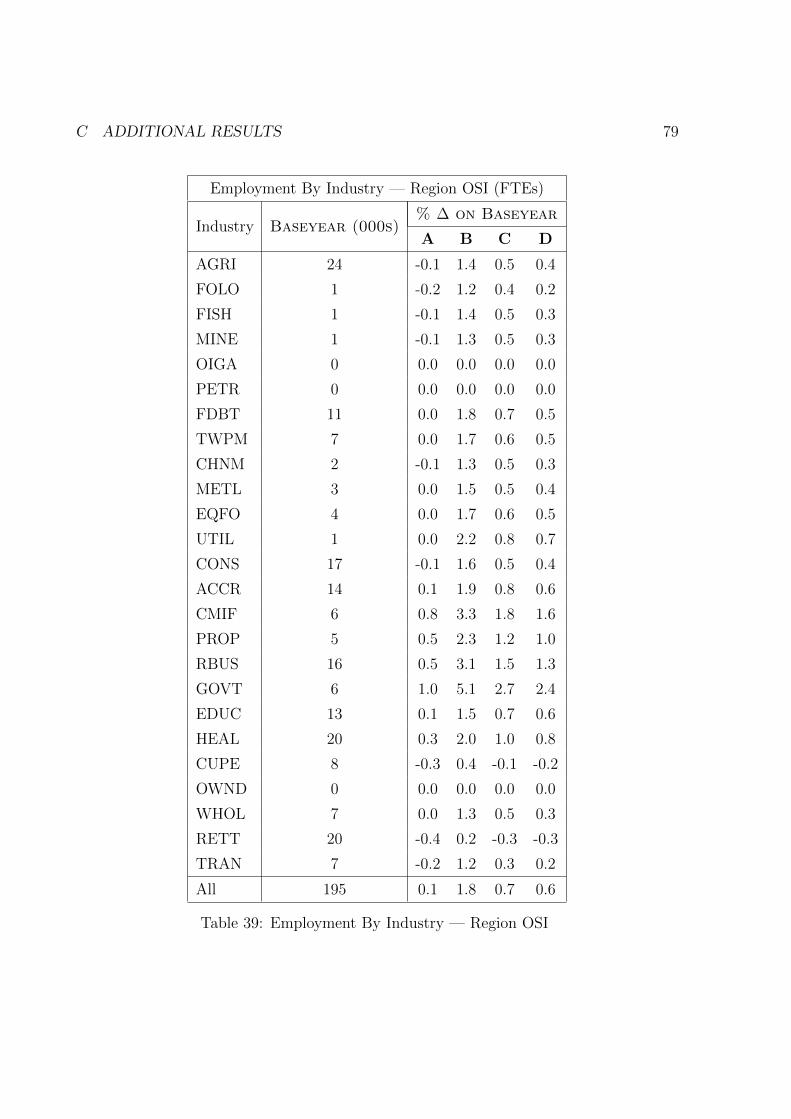
C ADDITIONAL RESULTS 79
Employment By Industry — Region OSI (FTEs)
Industry Baseyear (000s)% ∆ on Baseyear
A B C D
AGRI 24 -0.1 1.4 0.5 0.4
FOLO 1 -0.2 1.2 0.4 0.2
FISH 1 -0.1 1.4 0.5 0.3
MINE 1 -0.1 1.3 0.5 0.3
OIGA 0 0.0 0.0 0.0 0.0
PETR 0 0.0 0.0 0.0 0.0
FDBT 11 0.0 1.8 0.7 0.5
TWPM 7 0.0 1.7 0.6 0.5
CHNM 2 -0.1 1.3 0.5 0.3
METL 3 0.0 1.5 0.5 0.4
EQFO 4 0.0 1.7 0.6 0.5
UTIL 1 0.0 2.2 0.8 0.7
CONS 17 -0.1 1.6 0.5 0.4
ACCR 14 0.1 1.9 0.8 0.6
CMIF 6 0.8 3.3 1.8 1.6
PROP 5 0.5 2.3 1.2 1.0
RBUS 16 0.5 3.1 1.5 1.3
GOVT 6 1.0 5.1 2.7 2.4
EDUC 13 0.1 1.5 0.7 0.6
HEAL 20 0.3 2.0 1.0 0.8
CUPE 8 -0.3 0.4 -0.1 -0.2
OWND 0 0.0 0.0 0.0 0.0
WHOL 7 0.0 1.3 0.5 0.3
RETT 20 -0.4 0.2 -0.3 -0.3
TRAN 7 -0.2 1.2 0.3 0.2
All 195 0.1 1.8 0.7 0.6
Table 39: Employment By Industry — Region OSI
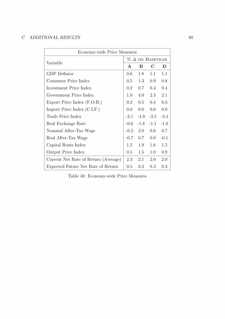
C ADDITIONAL RESULTS 80
Economy-wide Price Measures
Variable% ∆ on Baseyear
A B C D
GDP Deflator 0.6 1.8 1.1 1.1
Consumer Price Index 0.5 1.3 0.9 0.8
Investment Price Index 0.2 0.7 0.4 0.4
Government Price Index 1.0 4.0 2.3 2.1
Export Price Index (F.O.B.) 0.2 0.5 0.4 0.3
Import Price Index (C.I.F.) 0.0 0.0 0.0 0.0
Trade Price Index -2.1 -4.9 -3.5 -3.4
Real Exchange Rate -0.6 -1.8 -1.1 -1.0
Nominal After-Tax Wage -0.2 2.0 0.8 0.7
Real After-Tax Wage -0.7 0.7 0.0 -0.1
Capital Rents Index 1.5 1.9 1.6 1.5
Output Price Index 0.5 1.5 1.0 0.9
Current Net Rate of Return (Average) 2.3 2.1 2.0 2.0
Expected Future Net Rate of Return 0.5 0.3 0.3 0.3
Table 40: Economy-wide Price Measures

REFERENCES 81
References
Bacharach, M. (1970), Biproportional Matrices and Input-Output Change, Cambridge
University Press.
Dixon, P. B., Parmenter, B. R., Powell, A. A. & Wilcoxen, P. J. (1992), Notes and
Problems in Applied General Equilibrium Economics, North-Holland, New York.
Dixon, P. B., Parmenter, B. R., Sutton, J. & Vincent, D. P. (1982), ORANI: A Multisec-
toral Model of the Australian Economy, North-Holland, New York.
Dixon, P. B. & Rimmer, M. T. (2002), Dynamic General Equilibrium Modelling for Fore-
casting and Policy: A Practical Guide and Documentation of MONASH, Elsevier,
Amsterdam.
Jones, R. & Whalley, J. (1989), ‘A Canadian regional general equilibrium model and some
applications’, Journal of Urban Economics 25(3), 368–405.
Madden, J. R. (1990), FEDERAL: A Two-Region Multisectoral Fiscal Model of the Aus-
tralian Economy, PhD thesis, University of Tasmania, Australia.
McDougall, R. (1999), Entropy Theory and RAS are Friends, GTAP Working Paper 300,
Center for Global Trade Analysis, Department of Agricultural Economics, Purdue
University.
URL: http://ideas.repec.org/p/gta/workpp/300.html
Robson, N. (2012), A Multi-Regional Computable General Equilibrium Model for New
Zealand, PhD thesis, Victoria University of Wellington, New Zealand.
URL: http://researcharchive.vuw.ac.nz/handle/10063/2319
Related Documents