The Shooting-Room Paradox and Conditionalizing on Measurably Challenged Sets

PAUL BARTHA and CHRISTOPHER HITCHCOCK

THE SHOOTING-ROOM PARADOX AND CONDITIONALIZING ONMEASURABLY CHALLENGED SETS

ABSTRACT. We provide a solution to the well-known “Shooting-Room” paradox,developed by John Leslie in connection with his Doomsday Argument. In the “Shooting-Room” paradox, the death of an individual is contingent upon an event that has a 1/36chance of occurring, yet the relative frequency of death in the relevant population is 0.9.There are two intuitively plausible arguments, one concluding that the appropriate sub-jective probability of death is 1/36, the other that this probability is 0.9. How are thesetwo values to be reconciled? We show that only the first argument is valid for a standard,countably additive probability distribution. However, both lines of reasoning are legitimateif probabilities are non-standard. The subjective probability of death rises from 1/36 to0.9 by conditionalizing on an event that is not measurable, or whose probability is zero.Thus we can sometimes meaningfully ascribe conditional probabilities even when the eventconditionalized upon is not of positive finite (or even infinitesimal) measure.

In a dark corner of a hotel bar, several figures sporting name tags arehunched around a small table covered in empty beer bottles. One of thefigures is writing furiously on a napkin. The conversation is excited andconfused, as many try to speak at once. The individual words that do escapefrom the white noise of the bar are ominous: “. . . executioner. . . ”, “. . .doomsday. . . ”, “. . . double sixes and you die!”

Any participant in a recent philosophy conference is likely to haveencountered a scene much like this. Radical philosophers plotting the over-throw of civilization? No. They are merely curious thinkers testing theirmettle on a paradox of probability: the shooting-room paradox. In Section1.1 of this paper, we will describe this paradox and present the well-knownsolution to one part of it. In Section 1.2, we will sketch the solution to themore intransigent part of the paradox. The subsequent sections providethe mathematical details upon which the solution depends. We believe thatthese details are of interest in their own right, and may have applicationsin a number of philosophical problems.

Synthese118: 403–437, 1999.© 1999Kluwer Academic Publishers. Printed in the Netherlands.

404 PAUL BARTHA AND CHRISTOPHER HITCHCOCK

1. INTRODUCTION

1.1. The Ballad of George and Tracy

Imagine that our protagonist, George, has been called to a place knownthroughout the world as the Shooting-Room. There are dire consequencesfor those who do not heed the call. As he enters the room, he reads aportentous sign above the door:

Abandon all hope, you who enter this room!Well, not quite all hope – and here’s why:You’ve a 1/36 chance of meeting your doom,Yet 0.9 of those entering will die!

After George enters, a sinister figure at the front of the room – the “Exe-cutioner” – announces that he will roll two ordinary six-sided dice. If theresult is double sixes, George (and anyone else in the room with George)will be executed. This explanation seems to entail that George has a one inthirty-six chance of dying. Puzzle: how can the executioner’s explanationbe reconciled with the statement that 90% of those entering will die?

Here are some hints: (1) The world in which George lives has a count-ably infinite population. (2) The shooting room has movable walls, so thatit can be expanded to arbitrarily large size. (3). The executioner is immor-tal. (4) The last sentence of the verse above the door is not guaranteed tobe true: there is a possibility that it will not be true, but the probabilityof this eventuality coming to pass is zero (just as it is possible that a cointossed infinitely many times will never land heads, although there is zeroprobability that this will happen).

Still stumped? Here is the solution: the shooting-room game is played inrounds. In each round, a larger number of people is called to the shootingroom. In the first round, only one person is called; in the second roundnine; in the third round ninety; and in each successive round, ten times thenumber of people called for the preceding round. The game ends only ifand when double six is rolled in a given round, in which case all those inthe chamber in the last round are executed.1 There is a probability of onethat double sixes will eventually be rolled, and when that occurs, exactlyninety percent of those who have ever entered the room will be present inthe final, fatal, round of the game.2

This puzzle contains an important moral about the relationship betweensingle-case probabilities and frequencies: we can only expect the latter toconform to the former when (1) individual events (in this case the execu-tion or acquittal of those who enter the shooting-room) are probabilisticallyindependent; and (2) stopping times are probabilistically independent of

THE SHOOTING-ROOM PARADOX 405

frequencies. The latter restriction presents genuine problems in drug test-ing, for example, when ethical considerations mandate the continuation oftreatments that appear beneficial, and the termination of treatments that donot.

The apparent paradox was resolved by noting that single case prob-abilities and predicted frequencies need not coincide. We may recast theparadox, however, in such a way that the values 1/36 and 0.9 both appearto be rational subjective probabilities. Here’s how. Suppose that Georgeenters the shooting-room as before, and that he understands the mechanismof the game completely. What should be George’s subjective probabilityfor the proposition that he is executed, given that he has been selected toenter the chamber? The answer must be 1/36, for George knows that hewill die if and only if the result of a throw of two fair dice is double sixes.Assuming that he can compute that the chance of this outcome is 1/36, thathe has no other relevant information, and that his subjective probabilitiesare guided by his beliefs about chances,3 his subjective probability shouldbe 1/36.

Now suppose that George’s mother, Tracy, also understands the mech-anism of the game, knows that George was selected to enter the chamber,and hears the news that the game has ended. She does not know, however,whether George survived. What should be her subjective probability forGeorge to have died? This time, a reasonable answer is 0.9. Tracy knowsthat a finite number of people entered the room, George among them. Ofthose people, 90% died (or perhaps 100%, if the game ended on the firstround). Tracy has no additional information that is relevant to whether ornot George was one of those who participated in the final round, and hencedied, so Tracy’s subjective probability that George dies should be 0.9.

George and Tracy have exactly the same information, namely thatGeorge participated in the game. Neither knows on which round Georgewas selected (we may assume that George was blindfolded, althoughin fact this does not matter); neither knows how the dice came up onGeorge’s round. How then can the probabilities for George and Tracy beso different?

1.2. Sketch of the Solution

The previous paragraph contains a little white lie. George and Tracy do nothave exactly the same information: Tracy knows that the game has ended,but George does not. On the one hand, this seems crucial to the formulationof the paradox: when George phones Tracy to tell her that he is in the room,and that the executioner is about to roll the dice, it seems that her probabil-ity for George’s demise (before she learns that the game has ended) should


be only 1/36, the same as George’s. On the other hand, it is hard to see howthe additional information that the game has come to an end could matter:given that both George and Tracy understand the mechanism of the game,they should both assign probability one to the proposition that it eventuallyends. Conditioning on a proposition with probability one does not changeone’s probability assignments, so this extra piece of information couldhardly have raised Tracy’s subjective probability from 1/36 to 0.9.

It will be helpful, at this point, to make some additional assumptionsabout the manner in which individuals are selected to participate in theshooting-room game. Assume that each member of the population is as-signed a distinct natural number at random: we will call these numbers‘draft’ numbers.4 These numbers are known only to the executioner; how-ever, people know that they will be called no more than once. Individualsare called to the shooting room in the order of their draft numbers. Thus thefirst group to enter the room will consist of individual number 1; the secondgroup will consist of individuals 2–10; then 11–100 and so on. In general,9 · 10n−2 people are selected at roundn for n > 1. Before George is calledto participate in the game, both George and Tracy have prior probabilitiesfor propositions of the form: George has been assigned draft numberi. Letus assume that George and Tracy have the same priors: a difference in theirposterior probabilities (for George to die, upon learning that he participatesin the game) would hardly constitute a paradox if they began with differentpriors.

Suppose that the subjective probability function initially shared byGeorge and Tracy is standard and countably additive. It follows that theycannot assign uniform probabilities to propositions of the form: Georgehas draft numberi. The sum of these prior probabilities must be equal toone, since the probability thatGeorge has some draft numberis one. Forexample, it could be that the probability that George has draft numberi is2−i , since 1/2 + 1/4 + 1/8 +· · · sums to 1. However, the probability thatGeorge has draft numberi could not be equal to any constantk. For ifk = 0, then the ‘probability’ thatGeorge has some draft numberis 0 + 0 +0 + · · · = 0; whereas ifk > 0, the ‘probability’ thatGeorge has some draftnumberis k+ k+ k+ · · · = ∞. So the prior probabilities that George hasdraft numberi must converge to 0 asi approaches∞.

In the case of a countably additive probability function, then, the ar-gument for assigning a value of 0.9 to Tracy’s probability that Georgedies is fallacious. In particular: the statement, “Tracy has no additionalinformation that is relevant to whether or not George was one of thosewho participated in the final round, and hence died”, is false. Tracy’spriors provide such information: of necessity, they will be biased toward


early draft picks. In Section 2, we demonstrate that no matter what Tracy’sinitial prior probability is, so long as it is countably additive, it must bebiased toward early draft numbers in exactly the manner necessary for herposterior probability for George’s death to equal 1/36.

De Finetti took this sort of case to provide an argument against therequirement of countable additivity for probabilities.5 He reasoned that itought to be possible to have a lottery in which a countably infinite num-ber of tickets is issued, and that a rational agent should not be prohibitedfrom assigning equal probability to each ticket’s winning. Presumably, theoriginal intuition supporting Tracy’s assignment of 0.9 was based on theassumption that her beliefs about the draft lottery were of this sort. InSections 3 and 4, we use nonstandard analysis to construct a probabilitydistribution wherein George does have an equal (infinitesimal) probabilityof receiving each draft number. In this case the frequency argument forwhy Tracy should assign a 0.9 probability for George’s demise upon learn-ing that the game has ended stands up. In this setting, Tracy’s learning thatthe game has ended does make an impact upon her subjective probabilityfunction, even though her prior probability for this eventuality was one.The reason is that she is already conditionalizing on George’s being selec-ted to participate in the game, and as we shall see below this event musteither have probability zero, or be non-measurable.6

The problem is thus a special case of attempting to define a conditionalprobabilityP(A/B) whereB is ‘measurably challenged’, i.e., not of pos-itive measure. This means thatP(B) = 0 or thatB is non-measurable.WhileP(A/B) is typically defined as the ratioP(A·B)/P (B), it is usuallyleft undefined ifB is measurably challenged.7 However, there are cases inwhich P(B) = 0, but it is intuitively clear that a conditional probabilityfunctionP(·/B) exists.8 (For detailed arguments on this matter, see Hájek(1999).)

As a particularly simple example, suppose that we are throwing darts ata square grid that measures one meter by one meter. Due to poor aim, thevery point of the dart is equally likely to hit any point on the grid. Moreprecisely, any two regions of equal area are equally likely to contain thepoint where the dart hits. LetM be the horizontal line separating the topand bottom half of the grid; in terms of the coordinate system with origin atthe bottom left,M is the set of all points(x, y) with y = 1/2. There is zeroprobability that a dart will land exactly along this line. Now letL be the lefthalf of the grid, the set of points withx ≤ 1

2. What is the value ofP(L/M),the probability that the dart lands in the regionL given that it lands on theline M? Intuitively, the answer is 1/2, even though bothP(L · M) andP(M) are zero, so that the ratioP(L ·M)/P (M) is undefined.


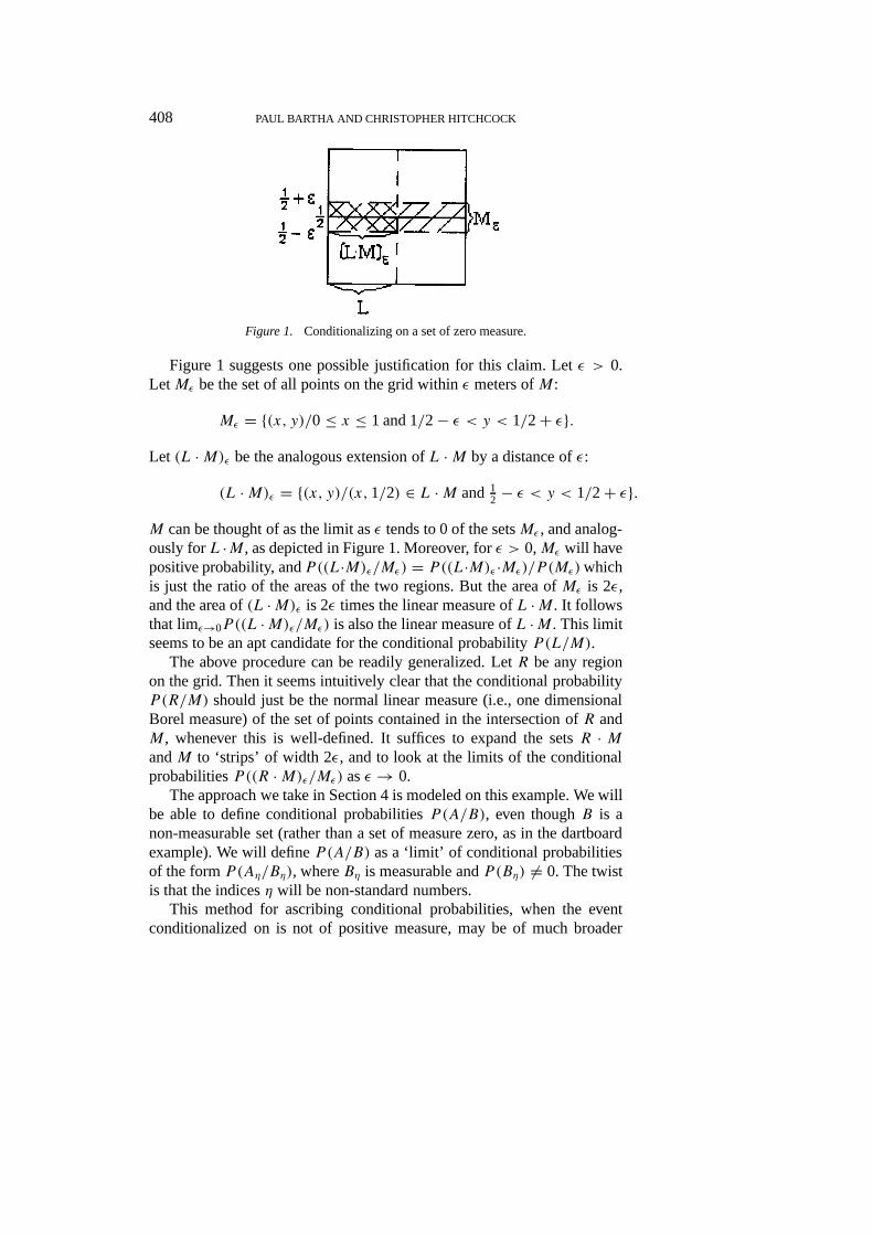
Figure 1. Conditionalizing on a set of zero measure.

Figure 1 suggests one possible justification for this claim. Letε > 0.LetMε be the set of all points on the grid withinε meters ofM:

Mε = {(x, y)/0 ≤ x ≤ 1 and 1/2− ε < y < 1/2+ ε}.Let (L ·M)ε be the analogous extension ofL ·M by a distance ofε:

(L ·M)ε = {(x, y)/(x,1/2) ∈ L ·M and 12 − ε < y < 1/2+ ε}.

M can be thought of as the limit asε tends to 0 of the setsMε , and analog-ously forL ·M, as depicted in Figure 1. Moreover, forε > 0,Mε will havepositive probability, andP((L·M)ε/Mε) = P((L·M)ε ·Mε)/P (Mε)whichis just the ratio of the areas of the two regions. But the area ofMε is 2ε,and the area of(L ·M)ε is 2ε times the linear measure ofL ·M. It followsthat limε→0P((L ·M)ε/Mε) is also the linear measure ofL ·M. This limitseems to be an apt candidate for the conditional probabilityP(L/M).

The above procedure can be readily generalized. LetR be any regionon the grid. Then it seems intuitively clear that the conditional probabilityP(R/M) should just be the normal linear measure (i.e., one dimensionalBorel measure) of the set of points contained in the intersection ofR andM, whenever this is well-defined. It suffices to expand the setsR · MandM to ‘strips’ of width 2ε, and to look at the limits of the conditionalprobabilitiesP((R ·M)ε/Mε) asε → 0.

The approach we take in Section 4 is modeled on this example. We willbe able to define conditional probabilitiesP(A/B), even thoughB is anon-measurable set (rather than a set of measure zero, as in the dartboardexample). We will defineP(A/B) as a ‘limit’ of conditional probabilitiesof the formP(Aη/Bη), whereBη is measurable andP(Bη) 6= 0. The twistis that the indicesη will be non-standard numbers.

This method for ascribing conditional probabilities, when the eventconditionalized on is not of positive measure, may be of much broader


value in addressing problems of philosophical concern. For example, oneobjection to probabilistic approaches to epistemology is that they seem toendorse a certain form of dogmatism: an agent who assigns probabilityone to some proposition must forever after assign probability one to thatproposition, no matter what else she may learn. Updating by condition-alization cannot dislodge such probability values. If, however, an agentis allowed to conditionalize on a proposition to which she did not previ-ously assign positive probability, she may be able to retract her previousassignment of maximum probability. This is precisely what happens in theshooting room paradox. Although George and Tracy begin by assigningprobability one to the proposition that the game will end, upon learning thatGeorge participates in the game, they are forced to revise their assignmentto a much lower probability (5/162 to be precise!).

1.3. Notation and Assumptions

In order to set up the mathematics of the problem, we introduce someuseful notation:

Ln The game has lengthn.

Rn George is selected to enter the room at roundn of thegame.

G George is selected to enter the room at some round of thegame.

Ni George is assigned draft numberi.

D George dies.

F The game finishes with a roll of double six. (Given theother assumptions, this means the game is finite.)

pi = P(Ni) (the prior probability for both George and Tracy thatGeorge has draft numberi).

rn =∑10n−1

i=1 pi (the prior probability that George is among the 10n−1

people chosen by roundn). It is also appropriate to setr0 = 0.

Recall thatP stands for the probability function representing George andTracy’s degrees of belief (which are taken to be identical).

In addition to the assumptions enumerated in Section 1.2, we assumein what follows that the dice rolls and the assignment of draft numbers areindependent, or rather that George and Tracy believe this to be the case.More precisely, this is the assumption that

P(Ni/Ln) = P(Ni)


for all i andn.9

1.4. The Problem

Recall that when George enters the shooting room, the information helearns (and on which he conditions) is just that he has been selected to enterthe room, which we signify byG. Tracy, by contrast, learns that Georgeis a participant and that the game finishes, i.e.,G · F . The two conditionalprobabilities of interest are thus

• P(D/G) = George’s posterior probability of dying, given George’sinformation (that he has been selected to enter); and• P(D/G · F) = George’s posterior probability of dying, given Tracy’s

information (that George has been selected and the game finishes).

Assuming for the moment that these conditional probabilities are bothwell-defined, then the difficulty is that they should be equal; for condi-tionalizing on an event with probability one makes no difference, andP(F) = 1. Indeed,P(F) is obtained by summing the probabilities thatthe first double-six occurs at rounds 1, 2, 3. . . :

(1/36)+ (35/36)(1/36) + (35/36)2(1/36)+ · · ·

= (1/36)×(

1

1− 35/36

)= 1.

So it appears that the two posterior probabilitiesP(D/G) andP(D/G·F)should be equal (if defined).

We divide the analysis into two cases. In the first case (Section 2), theprobability function is a standard, countably additive one. In the secondcase (Sections 3 and 4), the probabilities are non-standard.

2. COUNTABLY ADDITIVE CASE

First suppose that the prior probability function is countably additive.Countable additivity is a standard assumption applied to probability meas-ures. It means that ifE1, E2, . . . are mutually exclusive (so thatP(Ei ·Ej) = 0 for all i 6= j ), then

P(E1 ∨ E2 ∨ · · ·) =∞∑n=1

P(En).

In this case, it is false that your mother should assign probability 0.9 toyour dying upon reading your name in the paper. As explained in Section


1.2, this number depends upon the assumption that George is equally likelyto be assigned any draft number. The assumption is false, because the priorprobabilities must converge to 0 as the draft numbers become large.

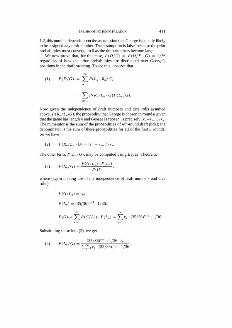
We now prove that, for this case,P(D/G) = P(D/F · G) = 1/36regardless of how the prior probabilities are distributed over George’spositions in the draft ordering. To see this, observe that

P(D/G) =∞∑n=1

P(Ln · Rn/G)(1)

=∞∑n=1

P(Rn/Ln ·G)P (Ln/G).

Now given the independence of draft numbers and dice rolls assumedabove,P(Rn/Ln·G), the probability that George is chosen in roundn giventhat the game has lengthn and George is chosen, is precisely(rn−rn−1)/rn.

The numerator is the sum of the probabilities ofnth-round draft picks; thedenominator is the sum of these probabilities for all of the firstn rounds.So we have

P(Rn/Ln ·G) = (rn − rn−1)/rn.(2)

The other term,P(Ln/G), may be computed using Bayes’ Theorem:

P(Ln/G) = P(G/Ln) · P(Ln)P (G)

,(3)

where (again making use of the independence of draft numbers and dicerolls)

P(G/Ln) = rn;

P(Ln) = (35/36)n−1 · 1/36;

P(G) =∞∑n=1

P(G/Ln) · P(Ln) =∞∑n=1

rn · (35/36)n−1 · 1/36.

Substituting these into (3), we get

P(Ln/G) = (35/36)n−1 · 1/36 · rn∑∞j=1 rj · (35/36)j−1 · 1/36

.(4)


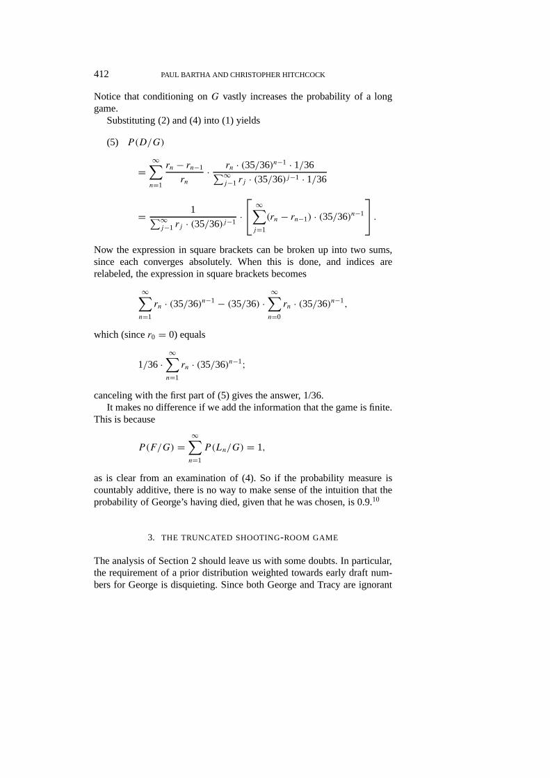
Notice that conditioning onG vastly increases the probability of a longgame.

Substituting (2) and (4) into (1) yields

P(D/G)(5)

=∞∑n=1

rn − rn−1

rn· rn · (35/36)n−1 · 1/36∑∞

j−1 rj · (35/36)j−1 · 1/36

= 1∑∞j−1 rj · (35/36)j−1

· ∞∑j=1

(rn − rn−1) · (35/36)n−1

.Now the expression in square brackets can be broken up into two sums,since each converges absolutely. When this is done, and indices arerelabeled, the expression in square brackets becomes

∞∑n=1

rn · (35/36)n−1 − (35/36) ·∞∑n=0

rn · (35/36)n−1,

which (sincer0 = 0) equals

1/36 ·∞∑n=1

rn · (35/36)n−1;

canceling with the first part of (5) gives the answer, 1/36.It makes no difference if we add the information that the game is finite.

This is because

P(F/G) =∞∑n=1

P(Ln/G) = 1,

as is clear from an examination of (4). So if the probability measure iscountably additive, there is no way to make sense of the intuition that theprobability of George’s having died, given that he was chosen, is 0.9.10

3. THE TRUNCATED SHOOTING-ROOM GAME

The analysis of Section 2 should leave us with some doubts. In particular,the requirement of a prior distribution weighted towards early draft num-bers for George is disquieting. Since both George and Tracy are ignorant


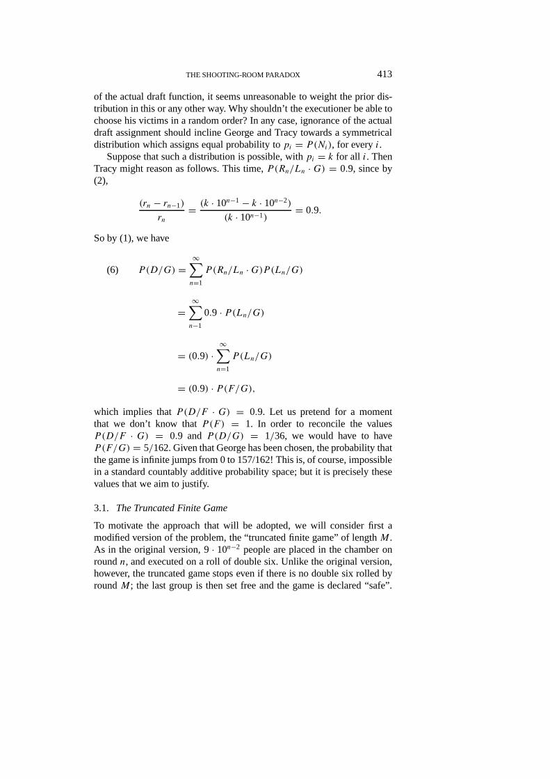
of the actual draft function, it seems unreasonable to weight the prior dis-tribution in this or any other way. Why shouldn’t the executioner be able tochoose his victims in a random order? In any case, ignorance of the actualdraft assignment should incline George and Tracy towards a symmetricaldistribution which assigns equal probability topi = P(Ni), for everyi.

Suppose that such a distribution is possible, withpi = k for all i. ThenTracy might reason as follows. This time,P(Rn/Ln · G) = 0.9, since by(2),

(rn − rn−1)

rn= (k · 10n−1 − k · 10n−2)

(k · 10n−1)= 0.9.

So by (1), we have

P(D/G) =∞∑n=1

P(Rn/Ln ·G)P (Ln/G)(6)

=∞∑n−1

0.9 · P(Ln/G)

= (0.9) ·∞∑n=1

P(Ln/G)

= (0.9) · P(F/G),which implies thatP(D/F · G) = 0.9. Let us pretend for a momentthat we don’t know thatP(F) = 1. In order to reconcile the valuesP(D/F · G) = 0.9 andP(D/G) = 1/36, we would have to haveP(F/G) = 5/162. Given that George has been chosen, the probability thatthe game is infinite jumps from 0 to 157/162! This is, of course, impossiblein a standard countably additive probability space; but it is precisely thesevalues that we aim to justify.

3.1. The Truncated Finite Game

To motivate the approach that will be adopted, we will consider first amodified version of the problem, the “truncated finite game” of lengthM.As in the original version, 9· 10n−2 people are placed in the chamber onroundn, and executed on a roll of double six. Unlike the original version,however, the truncated game stops even if there is no double six rolled byroundM; the last group is then set free and the game is declared “safe”.


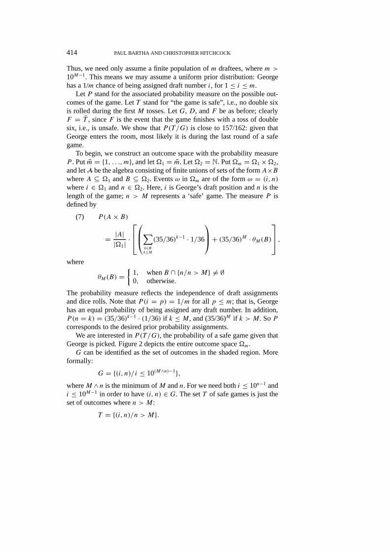
Thus, we need only assume a finite population ofm draftees, wherem >

10M−1. This means we may assume a uniform prior distribution: Georgehas a 1/m chance of being assigned draft numberi, for 1≤ i ≤ m.

Let P stand for the associated probability measure on the possible out-comes of the game. LetT stand for “the game is safe”, i.e., no double sixis rolled during the firstM tosses. LetG, D, andF be as before; clearlyF = T , sinceF is the event that the game finishes with a toss of doublesix, i.e., is unsafe. We show thatP (T /G) is close to 157/162: given thatGeorge enters the room, most likely it is during the last round of a safegame.

To begin, we construct an outcome space with the probability measureP . Putm = {1, . . ., m}, and let�1 = m. Let�2 = N. Put�m = �1×�2,and letA be the algebra consisting of finite unions of sets of the formA×BwhereA ⊆ �1 andB ⊆ �2. Eventsω in �m are of the formω = (i, n)

wherei ∈ �1 andn ∈ �2. Here,i is George’s draft position andn is thelength of the game;n > M represents a ‘safe’ game. The measureP isdefined by

P(A× B)(7)

= |A||�1| ·∑

k∈Bk≤M

(35/36)k−1 · 1/36

+ (35/36)M · θM(B) ,

where

θM(B) ={

1, whenB ∩ {n/n > M} 6= ∅0, otherwise.

The probability measure reflects the independence of draft assignmentsand dice rolls. Note thatP(i = p) = 1/m for all p ≤ m; that is, Georgehas an equal probability of being assigned any draft number. In addition,P(n = k) = (35/36)k−1 · (1/36) if k ≤ M, and (35/36)M if k > M. SoPcorresponds to the desired prior probability assignments.

We are interested inP (T /G), the probability of a safe game given thatGeorge is picked. Figure 2 depicts the entire outcome space�m.G can be identified as the set of outcomes in the shaded region. More

formally:

G = {(i, n)/i ≤ 10(M∧n)−1},whereM ∧n is the minimum ofM andn. For we need bothi ≤ 10n−1 andi ≤ 10M−1 in order to have(i, n) ∈ G. The setT of safe games is just theset of outcomes wheren > M:

T = {(i, n)/n > M}.


Figure 2. The truncated finite game.

To computeP (T /G) = P(T ∩G)/P (G), we need to computeP(T ∩G)andP(G).

P(G) =M∑j=1

P(i ≤ 10j−1, n = j)+ P(i ≤ 10M−1, n > M)(8)

=M∑j=1

10j−1

m(35/36)j−1(1/36)+ 10M−1

m(35/36)M

= 1

36m

(350/36)M − 1

(350/36) − 1+ 1

10m

(350

36

)M

= 1

314m[(350/36)M − 1] + 1

10m

(350

36

)M.

P (T ∩G) = 10M−1

m(35/36)M = 1

10m(350/36)M .(9)

So dividing (9) by (8), we obtain

P (T /G) = 110314[1− ( 36

350)M] + 1

(10)

= 1162157− 10

314(36350)

M.

Notice that this number is independent of the population sizem, and clearlyconverges to 157/162 asM →∞.


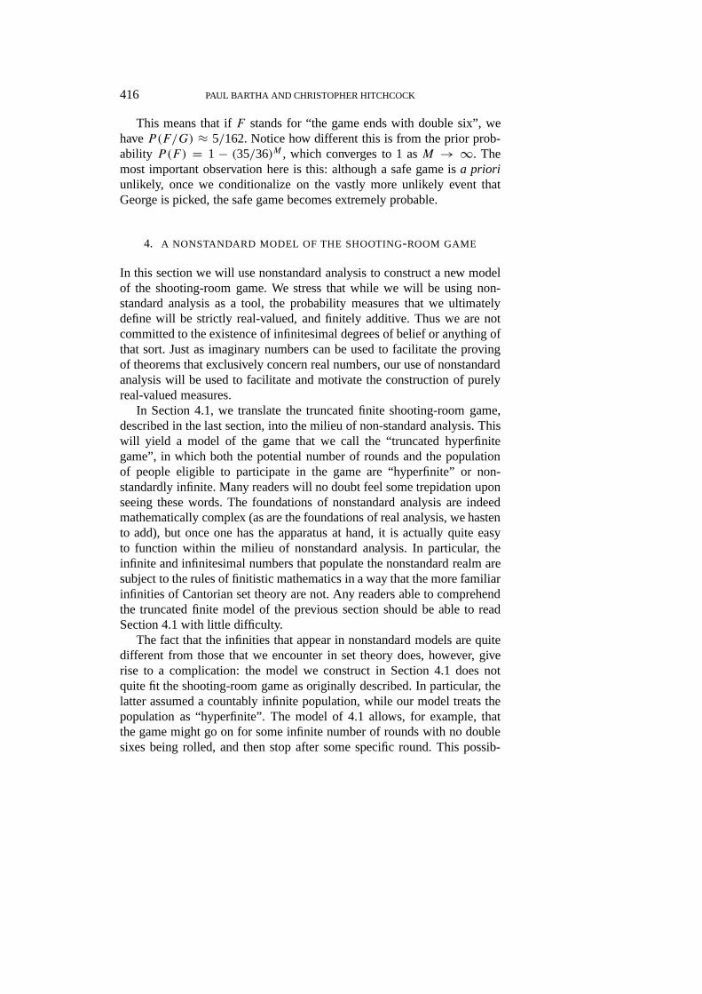
This means that ifF stands for “the game ends with double six”, wehaveP(F/G) ≈ 5/162. Notice how different this is from the prior prob-ability P(F) = 1− (35/36)M , which converges to 1 asM → ∞. Themost important observation here is this: although a safe game isa prioriunlikely, once we conditionalize on the vastly more unlikely event thatGeorge is picked, the safe game becomes extremely probable.

4. A NONSTANDARD MODEL OF THE SHOOTING-ROOM GAME

In this section we will use nonstandard analysis to construct a new modelof the shooting-room game. We stress that while we will be using non-standard analysis as a tool, the probability measures that we ultimatelydefine will be strictly real-valued, and finitely additive. Thus we are notcommitted to the existence of infinitesimal degrees of belief or anything ofthat sort. Just as imaginary numbers can be used to facilitate the provingof theorems that exclusively concern real numbers, our use of nonstandardanalysis will be used to facilitate and motivate the construction of purelyreal-valued measures.

In Section 4.1, we translate the truncated finite shooting-room game,described in the last section, into the milieu of non-standard analysis. Thiswill yield a model of the game that we call the “truncated hyperfinitegame”, in which both the potential number of rounds and the populationof people eligible to participate in the game are “hyperfinite” or non-standardly infinite. Many readers will no doubt feel some trepidation uponseeing these words. The foundations of nonstandard analysis are indeedmathematically complex (as are the foundations of real analysis, we hastento add), but once one has the apparatus at hand, it is actually quite easyto function within the milieu of nonstandard analysis. In particular, theinfinite and infinitesimal numbers that populate the nonstandard realm aresubject to the rules of finitistic mathematics in a way that the more familiarinfinities of Cantorian set theory are not. Any readers able to comprehendthe truncated finite model of the previous section should be able to readSection 4.1 with little difficulty.

The fact that the infinities that appear in nonstandard models are quitedifferent from those that we encounter in set theory does, however, giverise to a complication: the model we construct in Section 4.1 does notquite fit the shooting-room game as originally described. In particular, thelatter assumed a countably infinite population, while our model treats thepopulation as “hyperfinite”. The model of 4.1 allows, for example, thatthe game might go on for some infinite number of rounds with no doublesixes being rolled, and then stop after some specific round. This possib-


ility of stopping after some infinite number of rounds seems alien to ournormal way of thinking about infinity. We do not believe that this wouldbe too high a price to pay for a solution to the shooting-room paradox,but fortunately, we do not have to pay it. In Sections 4.2 and 4.3, wegradually convert the “truncated hyperfinite game” of Section 4.1 back intoa standard model of the game, where the number of potential rounds and ofpotential participants is countably infinite. On our way there, we will con-struct a “semi-standard” game where the population is hyperfinite, but thenumber of rounds in the game is standard, i.e., potentially countably infin-ite. Sections 4.2 and 4.3 provide only an overview of this construction; themathematical details are relegated to Section 6. This material is somewhatmore technical, and those readers who do not wish to bother themselveswith the details of converting non-standard infinities to standard infinitiesmay skip Sections 4.2 and 4.3 with little loss of continuity.

We begin with a very brief review of nonstandard analysis. The centralconcept is the∗-transform (pronounced star-transform). This is a functionthat maps standard entities into their nonstandard counterparts. The do-main of this function is the set-theoretic hierarchy erected upon the realnumbers. This domain includes real numbers, sets of real numbers, rela-tions, functions, sequences, and so on. The image of some standard entitys under the∗-transform will be denoted∗s. For example, the set of standardnumbersN becomes the nonstandard set∗N. This entity will also be a set;it will not, however, just be the set of images of natural numbers under the∗-transform. (We will elaborate upon this fact momentarily.) Indeed, thislatter set{∗n/n ∈ N} (which it is convenient to refer to asN, even thoughit is not, strictly, a standard entity) is not the∗-transform of any standardentity.

This latter observation points to an important distinction betweenin-ternal andexternalnonstandard entities. The definition of internal entitiesis complex, but roughly speaking, an entity is internal if it belongs to aset which is the image of some standard entity under the∗-transform;otherwise, it isexternal.11 N is an external set; intuitively, from the per-spective of nonstandard analysis, this is not a natural set of numbers, butmore of a set-theoretic gerrymander. In general, Cantorian infinities arevery different from nonstandard infinities, and the two mesh together veryawkwardly.

For illustrative purposes, we give an oversimplified and unrigorousanalogy. (Those curious about the rigorous details should consult Hurdand Loeb 1985, chapters 1 and 2.) Let∗ map each real number onto anequivalence class of sequences of real numbers.∗n will be the equivalenceclass of〈n, n, . . .〉, or [〈n, n, . . .〉]. Two sequences will be equivalent if


their terms are identical in ‘enough’ positions. We will not say preciselywhat ‘enough’ means, but if two sequences agree in all but finitely manyplaces, they agree in ‘enough’ places.

More generally, the∗-transform of a standard number-theoretic prop-erty will hold of a nonstandard number if, for one of its representativesequences, that property holds for ‘enough’ standard numbers in the se-quence. Consider, for example, the sequence〈1,2,3,4, . . .〉. Since eachterm in this sequence belongs toN, [〈1,2,3, . . .〉] will belong to∗N. Note,however, that[〈1,2,3, . . .〉] is not equal to∗n for any standard naturalnumbern. Indeed,[〈1,2,3, . . .〉] is larger than any such number, sinceall but finitely many of the terms of the sequence are larger thann. Thus[〈1,2,3, . . .〉] is infinite, or more properly,hyperfinite. To see that such hy-perfinite numbers are different from Cantorian infinite numbers, the readershould convince herself that there is no smallest hyperfinite number. Ana-logously, the number[〈1,1/2,1/3, . . .〉], is greater than zero, yet smallerthan any real number. Such numbers areinfinitesimal. The ∗-transformsof the normal mathematical operations of addition, subtraction, multiplic-ation and division are all well-defined on hyperfinite and infinitesimalnumbers. The reader may confirm, for instance that the product of thesetwo nonstandard numbers is∗1.

Finally, we state two very useful facts. First, any finite non-standard realnumber can be decomposed into the sum of a finite real number, knownas itsstandard part, and an infinitesimal number.12 We write ◦η for thestandard part ofη. Second, lets = s1, s2, . . . be a sequence of standardnumbers that converges to limitn. Formally, s is a function defined onthe natural numbers. Then∗s will be a function on∗N such that for everyhyperfinite argumentη, sη differs from n by at most an infinitesimal. Inother words, a standard sequence converges to a value if and only if itsnonstandard counterpart gets (and stays) infinitely close to that value.

4.1. The Truncated Hyperfinite Game

We first construct a non-standard version of the truncated game. Insteadof stopping the game after a finite number of rounds, however, we stop ifno double six occurs in the firstη rounds, whereη is an infinite integer in∗N\N. Instead of a countable population, we now need to assume a hyper-finite population of sizem, for some fixedmε∗N,m ≥ 10η−1. This allowsus to define a uniform probability distribution for the draft assignments.As in Section 3.1, we will construct a (non-standard) probability measuresuch that George has equal probability 1/m of being assigned any place inthe draft.


The outcome space is�m = �1 × �2, where�1 = m and�2 = ∗N.13

The algebraA consists of hyperfinite unions of setsA × B whereA is aninternal subset of�1 andB is an internal subset of�2.

Again, we writeω = (i, n) for elements of�m, wherei ∈ �1 andn ∈ �2. A safe game is represented by the conditionn > η. We define anon-standard measureµη on the algebraA by analogy with the definitionfor the truncated finite game

µη(A× B)(11)

= |A||�1| ·∑k∈Bk≤η

(35/36)k−1 · 1/36

+ (35/36)η · θη(B) ,

where|A| is the internal cardinality ofA and

θη(B) ={

1, whenB ∩ {n/n > η} 6= ∅0, otherwise.

Then(�m,A, µη) is the internal probability space for the truncated gameof lengthη. Although the measureµη depends on the choice ofη, we shallrefer to it asµ for the remainder of this section, sinceη is held constant.As before,µ({(i, n)/i = p}) = 1/m for all p ≤ m, soµ gives us therequired uniform distribution over draft positions.

Once again, we are interested in obtainingP (T /G), George’s andTracy’s subjective probability of a safe game, given that George is picked.This value can be determined using the non-standard probabilityµ. Here,

G = {(i, n)/i ≤ 10(η∧n)−1}is the set of all outcomes in which George is picked, whereη ∧ n is theminimum ofη andn. Also,

T = {(i, n)/n > η}is the set of ‘safe’ games. These sets are analogous to their counterparts inthe truncated finite game of Section 3.1. Figure 3 provides a picture of theprobability space�m, letting the shaded region represent the outcomes inthe setG.

The calculations (8)–(10) proceed exactly as in the finite case, replacingM with η. In particular, if we writeµG for the conditional probabilityµ(·/G), thenµG is a non-standard measure onA, and we have

µ(G) = 1

314m[(350/36)η − 1] + 1

10m

(350

36

)η(12)


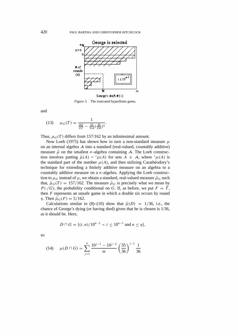
Figure 3. The truncated hyperfinite game.

and

µG(T ) = 1162157− 10

314(36350)

η.(13)

Thus,µG(T ) differs from 157/162 by an infinitesimal amount.Now Loeb (1975) has shown how to turn a non-standard measureµ

on an internal algebraA into a standard (real-valued, countably additive)measureµ on the smallestσ -algebra containingA. The Loeb construc-tion involves puttingµ(A) = ◦µ(A) for setsA ∈ A, where ◦µ(A) isthe standard part of the numberµ(A), and then utilizing Carathéodory’stechnique for extending a finitely additive measure on an algebra to acountably additive measure on aσ -algebra. Applying the Loeb construc-tion toµG instead ofµ, we obtain a standard, real-valued measureµG suchthat, µG(T ) = 157/162. The measureµG is precisely what we mean byP(·/G), the probability conditional onG. If, as before, we putF = T ,thenF represents an unsafe game in which a double six occurs by roundη. ThenµG(F ) = 5/162.

Calculations similar to (8)–(10) show thatµ(D) = 1/36, i.e., thechance of George’s dying (or having died) given that he is chosen is 1/36,as it should be. Here,

D ∩G = {(i, n)/10n−2 < i ≤ 10n−1 andn ≤ η},

so

µ(D ∩G) =η∑j=1

10j−1 − 10j−2

m

(35

36

)j−1 1

36(14)


= 0.9

36m

(350/36)η − 1

(350/36) − 1

= 0.9

314m[(350/36)η − 1].

Dividing (14) byµ(G) as given in (12), we obtain

0.9[1− (36/350)η](324/10) − (36/350)η

which has standard part 1/36.

4.2. The Semi-standard Game

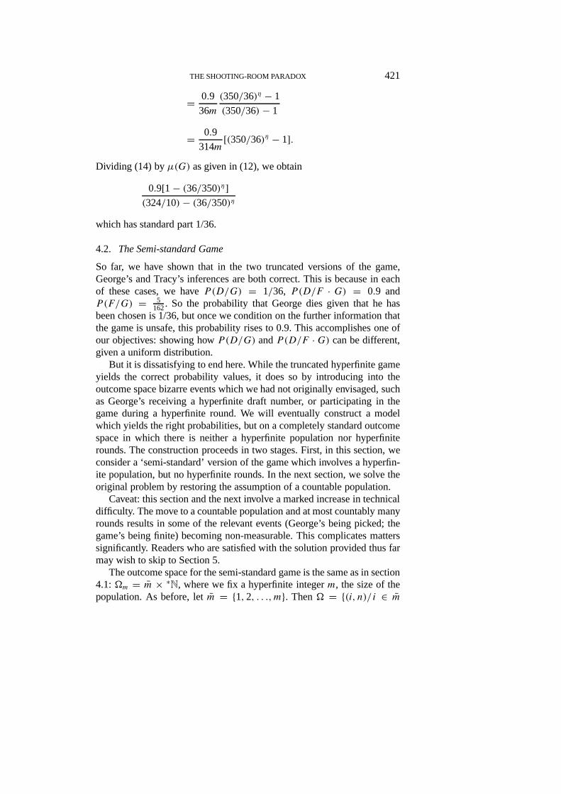
So far, we have shown that in the two truncated versions of the game,George’s and Tracy’s inferences are both correct. This is because in eachof these cases, we haveP(D/G) = 1/36, P(D/F · G) = 0.9 andP(F/G) = 5

162. So the probability that George dies given that he hasbeen chosen is 1/36, but once we condition on the further information thatthe game is unsafe, this probability rises to 0.9. This accomplishes one ofour objectives: showing howP(D/G) andP(D/F · G) can be different,given a uniform distribution.

But it is dissatisfying to end here. While the truncated hyperfinite gameyields the correct probability values, it does so by introducing into theoutcome space bizarre events which we had not originally envisaged, suchas George’s receiving a hyperfinite draft number, or participating in thegame during a hyperfinite round. We will eventually construct a modelwhich yields the right probabilities, but on a completely standard outcomespace in which there is neither a hyperfinite population nor hyperfiniterounds. The construction proceeds in two stages. First, in this section, weconsider a ‘semi-standard’ version of the game which involves a hyperfin-ite population, but no hyperfinite rounds. In the next section, we solve theoriginal problem by restoring the assumption of a countable population.

Caveat: this section and the next involve a marked increase in technicaldifficulty. The move to a countable population and at most countably manyrounds results in some of the relevant events (George’s being picked; thegame’s being finite) becoming non-measurable. This complicates matterssignificantly. Readers who are satisfied with the solution provided thus farmay wish to skip to Section 5.

The outcome space for the semi-standard game is the same as in section4.1:�m = m × ∗N, where we fix a hyperfinite integerm, the size of thepopulation. As before, letm = {1,2, . . ., m}. Then� = {(i, n)/i ∈ m


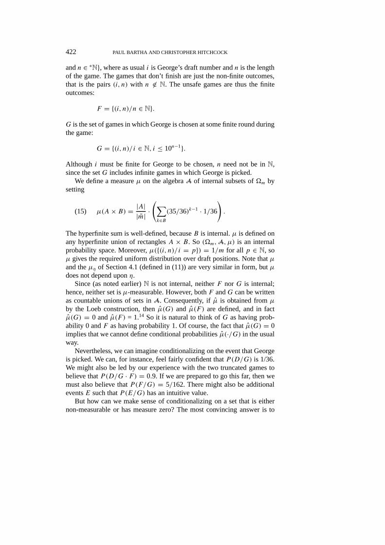
andn ∈ ∗N}, where as usuali is George’s draft number andn is the lengthof the game. The games that don’t finish are just the non-finite outcomes,that is the pairs(i, n) with n 6∈ N. The unsafe games are thus the finiteoutcomes:

F = {(i, n)/n ∈ N}.G is the set of games in which George is chosen at some finite round duringthe game:

G = {(i, n)/i ∈ N, i ≤ 10n−1}.Although i must be finite for George to be chosen,n need not be inN,since the setG includes infinite games in which George is picked.

We define a measureµ on the algebraA of internal subsets of�m bysetting

µ(A× B) = |A||m| ·(∑k∈B(35/36)k−1 · 1/36

).(15)

The hyperfinite sum is well-defined, becauseB is internal.µ is defined onany hyperfinite union of rectanglesA × B. So (�m,A, µ) is an internalprobability space. Moreover,µ({(i, n)/i = p}) = 1/m for all p ∈ N, soµ gives the required uniform distribution over draft positions. Note thatµ

and theµη of Section 4.1 (defined in (11)) are very similar in form, butµ

does not depend uponη.Since (as noted earlier)N is not internal, neitherF norG is internal;

hence, neither set isµ-measurable. However, bothF andG can be writtenas countable unions of sets inA. Consequently, ifµ is obtained fromµby the Loeb construction, thenµ(G) and µ(F ) are defined, and in factµ(G) = 0 andµ(F ) = 1.14 So it is natural to think ofG as having prob-ability 0 andF as having probability 1. Of course, the fact thatµ(G) = 0implies that we cannot define conditional probabilitiesµ(·/G) in the usualway.

Nevertheless, we can imagine conditionalizing on the event that Georgeis picked. We can, for instance, feel fairly confident thatP(D/G) is 1/36.We might also be led by our experience with the two truncated games tobelieve thatP(D/G · F) = 0.9. If we are prepared to go this far, then wemust also believe thatP(F/G) = 5/162. There might also be additionaleventsE such thatP(E/G) has an intuitive value.

But how can we make sense of conditionalizing on a set that is eithernon-measurable or has measure zero? The most convincing answer is to


demonstrate that we can actually construct a measureµG on an algebraAG of subsets of�m that has the required properties. The remainder ofthis section accomplishes this task; we stress that the construction here isthe key to the solution of the original problem.

We construct the algebraAG in such a way that forη ∈ ∗N\N, everyAin AG has a natural analogueAη in the algebra for the truncated hyperfinitegame of lengthη. In fact, eachA will be the ‘setwise limit’ of the setsAη,since the intersection overη ∈ ∗N\N of the set theoretic differencesA4Aηis empty. This means that there is nothing included in (excluded from)A

that is not eventually included in (excluded from) all setsAη, asη decreaseswithin ∗N\N.

Even though some of the sets inAG will not be internal, each setAηwill be an internal subset of�m. We show that the standard part of thequotient

µ(Aη ∩Gη)

µ(Gη)(16)

is constant for eachη, and define a conditional probability measureµG onAG by lettingµG(A) be this constant. This process gives us a well-defined,finitely additive probability measure on an algebra of sets.15

This strategy for defining the conditional probability is similar in spiritto the method described for the geometric example in the introduction.We expand bothA andG slightly to sets with a well-defined, non-zeroµ-measure, and take the standard parts of the quotients in (16). It turns outthat these standard parts are constant, which is the analogue of convergencein the truncated finite game.

The algebraAG and theη-mapping are constructed in Section 6.1; themeasureµG is constructed and proven to be well-defined in Section 6.2.We will here only summarize the properties ofµG:

• The measureµG is finitely additive on the algebraAG.• µG(F) = 5

162 which follows from the result (13) of Section 4.1. Thechance of a finite game is slim, given that George is picked.• µG(D) = 1

36, which follows from the discussion following (14) ofSection 4.1.• µG(D/F) = 0.9, which follows from the above results and the fact

thatµG(D/F ) = 0.

4.3. The Original Game

At last! We are finally ready to construct a measureνG which intuitivelycorresponds to conditionalizing on George’s being picked in the original


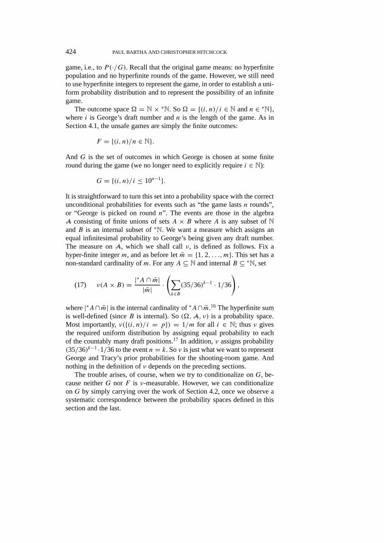
game, i.e., toP(·/G). Recall that the original game means: no hyperfinitepopulation and no hyperfinite rounds of the game. However, we still needto use hyperfinite integers to represent the game, in order to establish a uni-form probability distribution and to represent the possibility of an infinitegame.

The outcome space� = N × ∗N. So� = {(i, n)/i ∈ N andn ∈ ∗N},wherei is George’s draft number andn is the length of the game. As inSection 4.1, the unsafe games are simply the finite outcomes:

F = {(i, n)/n ∈ N}.And G is the set of outcomes in which George is chosen at some finiteround during the game (we no longer need to explicitly requirei ∈ N):

G = {(i, n)/i ≤ 10n−1}.It is straightforward to turn this set into a probability space with the correctunconditional probabilities for events such as “the game lastsn rounds”,or “George is picked on roundn”. The events are those in the algebraA consisting of finite unions of setsA × B whereA is any subset ofNandB is an internal subset of∗N. We want a measure which assigns anequal infinitesimal probability to George’s being given any draft number.The measure onA, which we shall callν, is defined as follows. Fix ahyper-finite integerm, and as before letm = {1,2, . . ., m}. This set has anon-standard cardinality ofm. For anyA ⊆ N and internalB ⊆ ∗N, set

ν(A× B) = |∗A ∩ m||m| ·

(∑k∈B(35/36)k−1 · 1/36

),(17)

where|∗A∩ m| is the internal cardinality of∗A∩ m.16 The hyperfinite sumis well-defined (sinceB is internal). So(�,A, ν) is a probability space.Most importantly,ν({(i, n)/i = p}) = 1/m for all i ∈ N; thusν givesthe required uniform distribution by assigning equal probability to eachof the countably many draft positions.17 In addition,ν assigns probability(35/36)k−1 ·1/36 to the eventn = k. Soν is just what we want to representGeorge and Tracy’s prior probabilities for the shooting-room game. Andnothing in the definition ofν depends on the preceding sections.

The trouble arises, of course, when we try to conditionalize onG, be-cause neitherG nor F is ν-measurable. However, we can conditionalizeonG by simply carrying over the work of Section 4.2, once we observe asystematic correspondence between the probability spaces defined in thissection and the last.


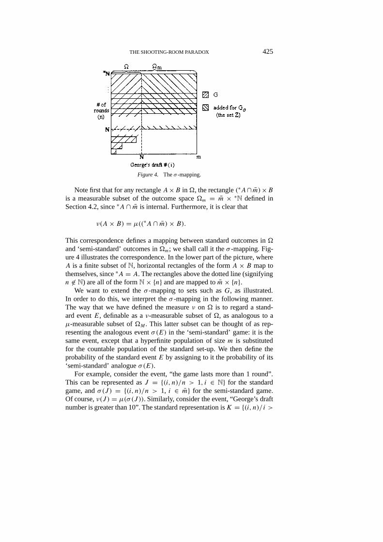
Figure 4. Theσ -mapping.

Note first that for any rectangleA×B in�, the rectangle(∗A∩ m)×Bis a measurable subset of the outcome space�m = m × ∗N defined inSection 4.2, since∗A ∩ m is internal. Furthermore, it is clear that

ν(A× B) = µ((∗A ∩ m)× B).

This correspondence defines a mapping between standard outcomes in�

and ‘semi-standard’ outcomes in�m; we shall call it theσ -mapping. Fig-ure 4 illustrates the correspondence. In the lower part of the picture, whereA is a finite subset ofN, horizontal rectangles of the formA × B map tothemselves, since∗A = A. The rectangles above the dotted line (signifyingn 6∈ N) are all of the formN× {n} and are mapped tom× {n}.

We want to extend theσ -mapping to sets such asG, as illustrated.In order to do this, we interpret theσ -mapping in the following manner.The way that we have defined the measureν on � is to regard a stand-ard eventE, definable as aν-measurable subset of�, as analogous to aµ-measurable subset of�M . This latter subset can be thought of as rep-resenting the analogous eventσ (E) in the ‘semi-standard’ game: it is thesame event, except that a hyperfinite population of sizem is substitutedfor the countable population of the standard set-up. We then define theprobability of the standard eventE by assigning to it the probability of its‘semi-standard’ analogueσ (E).

For example, consider the event, “the game lasts more than 1 round”.This can be represented asJ = {(i, n)/n > 1, i ∈ N} for the standardgame, andσ (J ) = {(i, n)/n > 1, i ∈ m} for the semi-standard game.Of course,ν(J ) = µ(σ (J )). Similarly, consider the event, “George’s draftnumber is greater than 10”. The standard representation isK = {(i, n)/i >


10, i ∈ N}; the semi-standard representation isσ (K) = {(i, n)/i > 10,i ∈ m}, and once againν(K) = µ(σ (K)).

The crucial next step is to extend the mappingσ between standard andsemi-standard events to non-measurable events – specifically, to those thatcan be represented in the algebraAG of Section 4.2. Most importantlywe want to establish analogues for the two events of greatest interest in theshooting-room game:F (the game finishes) andG (George is picked). Theanalysis is clearest forF . The ‘unsafe’ standard game

F = {(i, n)/n ∈ N, i ∈ N}

plainly corresponds to the unsafe semi-standard game

σ (F ) = {(i, n)/n ∈ N, i ∈ m}.

More problematically, the event of George’s being picked in the standardgame,

G = {(i, n)/i ∈ N and i ≤ 10n−1},

corresponds to George’s being picked in the non-standard game, whichhappens to beexactlythe same set:

σ (G) = {(i, n)/i ∈ N and i ≤ 10n−1}.

For even in the semi-standard game, George’s draft number must be inNif he is actually selected. Arguably, however,σ (G) should be the largerset pictured in Figure 4, since this is what we would get if we applied theσ -mapping one rectangle at a time.

This creates a technical difficulty, because we want to defineσ on abasis for an algebra of sets, and extend it inductively to the full algebra byputtingσ (A∩B) = σ (A)∩σ (B) andσ (A∪B) = σ (A)∪σ (B). In preciseterms, the difficulty is as follows. Consider the standard setG∩F of infinitegames in which George is not selected. In the standard game, this set isempty: George is assigned a finite draft number, so that he will eventuallybe selected in any infinite game. By contrast, in the semi-standard game,this set is not empty, since there are infinite games in which George isassigned a draft number inm\N.

In fact, if we letσ (G) andσ (F ) stand for the semi-standard outcomes,then

σ (G) ∩ σ (F ) = {(i, n)/i ∈ m\N, n ∈ ∗N\N};


we will call this setZ. The setZ is indicated in Figure 4. The difficulty,then, is that the mappingσ is not well-defined: the imageσ (∅) of theempty set∅ should again be the empty set, but by writing∅ = G ∩ F andapplying the inductive definition, we getσ (∅) = Z.

Fortunately, it is not too difficult to tidy upσ , because it turns out thatµG(Z) = 0, whereµG is the conditional probability defined in Section4.2. It should hardly be surprising that the probability of an infinite (semi-standard) game in which George isnot selected, given that Georgeisselected, is zero, and the proof is straightforward. BecauseZ is a set ofmeasure 0, we can simply tack it on in defining theσ -image. This willallow us to define the conditional probabilityνG for the standard game,on essentially the same algebra of sets as in Section 4.2. The details arecontained in Section 6.3.

We may thus define, forA in the algebraAG,

νG(A) = µG(σ (A)).18

This completes the construction of the probability measureνG, whichis intended to have the properties ofP(·/G), probability conditionalizedonG. The measure is finitely additive on the algebraAG.

It is worth briefly rehearsing the steps involved in evaluatingνG(A), forA ∈ AG.

Step 1: Theσ -mapping.First, we mapA, a subset of� = N× ∗N, toσ (A),the analogous subset of�m = m × ∗N. This sets up a correspondencebetween events in the standard game and events in the semi-standard game;the measureν on�, corresponds toµ on�m.

Step 2: Theη-mapping.Second, we modify bothσ (A) andG – neither ofwhich is likely to beη-measurable – by applying theη-mapping to bothsets (for suitably smallη ∈ ∗N\N). In effect, this sets up a correspondencebetween the semi-standard game and the truncated hyperfinite game ofSection 4.1. Theorem 1 assures us that the ratiosµ(σ (A)η ∩ Gη)/µ(Gη)

are constant (up to an infinitesimal difference).

Step 3: Conditionalization.νG(A) is defined as this constant ratio.

SinceµG(Z) = 0, we may carry over all important results from Section4.2. In particular, we have at last proved the results, which all follow fromthe discussion at the end of Section 4.2:

• νG(F ) = 5162.

• νG(D) = 136.


• νG(D/F) = 0.9.

5. CONCLUSION

In the countably additive case, there is no way to make sense of assigning asubjective probability of 0.9 to George’s demise – but the weakness of thisanalysis is its inability to accommodate the intuition that George is equallylikely to have any draft position. In the non-standard case, which allowsus to assign equal probability to each event in a countable partition, theabove analysis demonstrates that the crucial factor in determining whetherthe subjective probability of George’s dying is 1/36 or 0.9 is the possessionof knowledge about whether or not the game comes to an end.19

This only confirms what we all know: mother is always right, or atleast never wrong! George, like so many of his generation, was quick toaccuse his mother of worrying too much.20 But with experience (and a littlenonstandard analysis), George will soon come to realize that his mother’sfear for his life was justified after all.

6. CONSTRUCTIONS AND PROOFS

6.1. Construction ofAG and theη-mapping

In this section, we construct the familyAG and theη-mapping of Section4.2.

In what follows, we useφ to represent an arbitrary function fromNto N, andψ for the specific functionψ(n) = 10n−1. For any suchφ, putφ′(n) = φ(n) ∧ ψ(n), the minimum ofφ andψ . We shall say thatφ isof the same order asψ if lim n→∞φ(n)/ψ(n) exists; the limit is a non-negative real number. This condition will be abbreviated by writingφ is#ψ ; we will also write

φ(n)

ψ(n)∼ k

to mean that limn→∞φ(n)/ψ(n) = k. Note that if φ′ is #ψ , thenφ′(n)/ψ(n) ∼ k for somek with 0≤ k ≤ 1.

We start with abasisβ for the algebra, consisting of four types ofsubsets of�m.

1. Aφ = {(i, n)/i ≤ φ(n) andi ∈ N}, whereφ′ is#ψ .2. Aφ = {(i, n)/i > φ(n) or i 6∈ N}, whereφ′ is#ψ .


3. BS = {(i, n)/n ∈ S}, whereS ⊆ N is finite or co-finite.4. BS = {(i, n)/n 6∈ S}, whereS ⊆ N is finite or co-finite.

The algebraAG consists of all finite unions of finite intersections of setsin β. It is easy to verify that this set is closed under finite intersections,finite unions, and the taking of complements; hence, it is an algebra. Moststandard events of interest in the game can be expressed in terms of a setin this algebra. Sets of types 3 and 4 represent conditions on the length ofthe game, while in sets of type 1 and 2, the functionsφ are used to specifyranges of possible draft positions for George. For instance, 10n−2 < i ≤10n−1 represents the condition that George is chosen in the last round; theset of outcomes satisfying this condition isAφ ∩Aψ , whereφ(n) = 10n−2.

It is easy to check that the intersection of any two sets of the same typeis another set of that type. This is obvious for sets of type 3 or 4, and forthe first two types it is a consequence of the following Lemma.

LEMMA 1. If φ1 andφ2 are#ψ , then so areφ1 + φ2, |φ1 − φ2|, φ1 ∧ φ2,φ1 ∨ φ2 andk · φ1, for any constantk ∈ N. Here,∧ denotes minimum and∨ denotes maximum.

Proof. Supposeφ1(m)/ψ(n) ∼ a andφ2(n)/ψ(n) ∼ b. Then we canwrite φ1(n) = a · ψ(n) + α(n) andφ2(n) = b · ψ(n) + β(n), whereα(n)/ψ(n) ∼ 0 andβ(n)/ψ(n) ∼ 0. Since[α(n) + β(n)]/ψ(n) clearlyapproaches 0 asn→ ∞, this shows that[φ1(n)+ φ2(n)]/ψ(n) ∼ a + b.The other results are proved similarly. �

For sets of types 1 and 2, we allow only functionsφ such thatφ′ is #ψ .This is becauseφ′/ψ ∼ k if and only if ◦[φ′(η)/ψ(η)] = k for everyη ∈∗N\N,21 and it can be verified thatφ′ must satisfy this condition in orderfor µG(Aφ) to be defined.

The next step is to define, forη ∈ ∗N\N, theη-mapping which pairseach setA in AG with an internal subsetAη of �m. We first defineAη forthe four basic types of sets.

1. Aφ,η = {(i, n)/i ≤ φ(n ∧ η)}.2. Aφ,η = {(i, n)/i > φ(n ∧ η)}.3. BS,η = {(i, n)/n ∈ ∗S andn ≤ η}.22

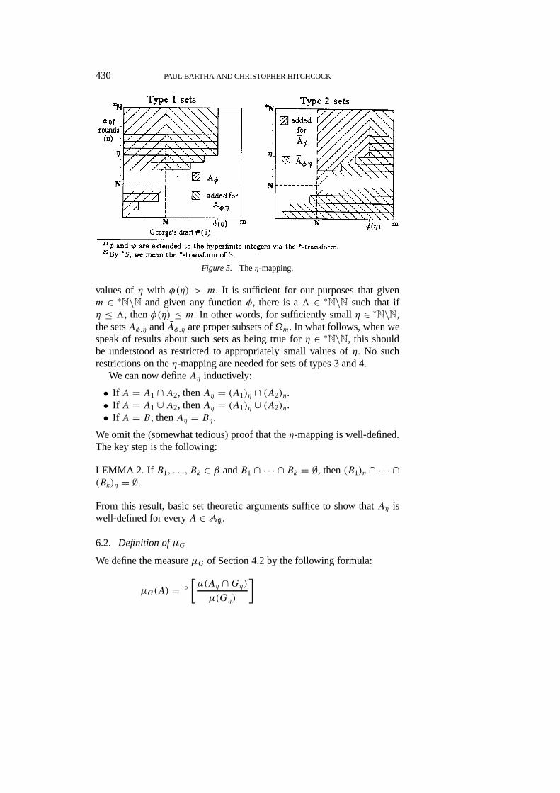
4. BS,η = {(i, n)/n 6∈ ∗S or n > η}.The following pictures illustrate the relation between sets of types 1 and2 in AG and their images under theη-mapping; similar relations exist fortypes 3 and 4. The pictures make it clear that for anyA ∈ AG, the setsAη‘converge setwise’ toA asη decreases within∗N\N.

Strictly speaking, for unbounded functionsφ, the setsAφ,η and Aφ,ηare not proper subsets of�m if η is sufficiently large, since there will be


Figure 5. Theη-mapping.

values ofη with φ(η) > m. It is sufficient for our purposes that givenm ∈ ∗N\N and given any functionφ, there is a3 ∈ ∗N\N such that ifη ≤ 3, thenφ(η) ≤ m. In other words, for sufficiently smallη ∈ ∗N\N,the setsAφ,η andAφ,η are proper subsets of�m. In what follows, when wespeak of results about such sets as being true forη ∈ ∗N\N, this shouldbe understood as restricted to appropriately small values ofη. No suchrestrictions on theη-mapping are needed for sets of types 3 and 4.

We can now defineAη inductively:

• If A = A1 ∩ A2, thenAη = (A1)η ∩ (A2)η.• If A = A1 ∪ A2, thenAη = (A1)η ∪ (A2)η.• If A = B, thenAη = Bη.

We omit the (somewhat tedious) proof that theη-mapping is well-defined.The key step is the following:

LEMMA 2. If B1, . . ., Bk ∈ β andB1 ∩ · · · ∩ Bk = ∅, then(B1)η ∩ · · · ∩(Bk)η = ∅.From this result, basic set theoretic arguments suffice to show thatAη iswell-defined for everyA ∈ AG.

6.2. Definition ofµG

We define the measureµG of Section 4.2 by the following formula:

µG(A) = ◦[µ(Aη ∩Gη)

µ(Gη)

]


for A ∈ AG, whenever this number is constant forη ∈ ∗N\N. We shallsay thatµG(A) is defined if this condition is satisfied. Sinceµ and theη-mapping are well-defined, so is the functionµG. Note thatG is just a ‘type1’ set, specificallyAψ whereψ(n) = 10n−1, so

Gη = {(i, n)/i ≤ ψ(n ∧ η)}.The following theorem states thatµG(A) is defined forA ∈ AG.

THEOREM 1. For everyA ∈ AG, there is a constant real numbera suchthat for everyη ∈ ∗N\N, ◦[µ(Aη ∩ Gη)/µ(Gη)] = a. That is,µG(A) isdefined and equal toa.

The theorem is proved first for the four basic types of setsA in AG, i.e.,for setsA in β.

1. SupposeA = Aφ , whereφ′(n)/10n−1 ∼ a. Thenφ′(n) = a10n−1 +α(n), whereα(n)/10n−1 ∼ 0. SinceAη ∩Gη = {(i, n)/i ≤ φ′(n∧ η)},we have (by the definition ofµ in (15))

µ(Aη ∩Gη) =η∑n=1

φ′(n)m

(35

36

)n−1 1

36+ φ

′(η)m

(35

36

)η(18)

=η∑n=1

a · 10n−1

m

(35

36

)n−1 1

36+ a · 10η−1

m

(35

36

)η

+η∑n=1

α(n)

m

(35

36

)n−1 1

36+ α(η)

m

(35

36

)η

= aµ(Gη)+η∑n=1

α(n)

m

(35

36

)n−1 1

36+ α(η)

m

(35

36

)η.

Sinceα(n)/10n−1 ∼ 0, given anyε > 0 we can find a finiteM suchthatα(n) ≤ ε · 10n−1 for n ≥ M. It follows that the second and thirdterms in (18) sum to less than

M∑n=1

α(n)

m

(35

36

)n−1 1

36+ ε · µ(Gη).

Hence, when we divide (18) byµ(Gη) and take the standard part, theresult is justa. SoµG(A) is defined and equalsa.


2. If A = Aφ , whereφ′(n)/10n−1 ∼ a, then it follows thatµG(A) isdefined and equals 1− a, since(Aφ,η ∩Gη) ∪ (Aφ,η ∩Gη) = Gη.

3. SupposeA = BS , whereS ⊆ N is finite or co-finite.

(a) If S is finite, then∗S = S, so thatAη = BS,η = BS. Now

BS ∩Gη = {(i, n)/i ≤ 10n−1, n ∈ S}.SupposeK is an upper bound forS, for some finiteK. Then

µ(Aη ∩Gη) =∑n∈S

10n−1

m

(35

36

)n−1 1

36

≤K∑n=1

10n−1

m

(35

36

)n−1 1

36

= 1

36m

[(350/36)K − 1

(350/36) − 1

],

and it is clear that◦[µ(Aη ∩Gη)/µ(Gη)] = 0 for everyη ∈ ∗N\N.SoµG(A) = 0 in this case.

(b) If S is co-finite, thenS = T for some finiteT . Then

Aη = BS,η = {(i, n)/n ≤ η, n 6∈ T }.So

Aη ∩Gη = {(i, n)/i ≤ 10n−1, n ≤ η, n 6∈ T }= {(i, n)/i ≤ 10n−1, n ≤ η}\{(i, n)/i ≤ 10n−1, n ∈ T }= (Fη ∩Gη)\(BT,η ∩Gη),

whereFη is the ‘unsafe’ setF of Section 3.2. There, we showedthat◦[µη(Fη ∩Gη)/µη(Gη)] = 5/162; the result also holds if wesubstituteµ for µη. SinceT is finite,◦[µ(BT,η∩Gη)/µ(Gη)] = 0,as just shown. Hence, for this case,µG(A) = 5/162.

4. Finally, supposeA = BS, whereS ⊆ N is either finite or co-finite.Then it follows from the above results thatµG(A) = 1 if S is finiteand 157/162 ifS is co-finite.

The next step is to prove that Theorem 1 holds ifA is a finite intersectionof sets inβ. Recall (from Lemma 1) that the intersection of any two setsof the same type is another set of the same type; it follows that we mayassume thatA is a finite intersection of at most four sets, one of each type.


Furthermore, ifS is finite andBS is in the intersection, then case 3 aboveshows thatµG(A) = 0. If S is a co-finite set, thenS ∩ T is co-finite ifT isfinite, and finite ifT is co-finite; this shows that we may assume that oneof the following cases holds: (i) the intersection contains no sets of type3 or 4; (ii) the intersection contains exactly one type 3 setBS whereS isco-finite, and no type 4 set; (iii) the intersection contains exactly one type4 set and no type 3 set. It is straightforward that if we can demonstrate thatµG(A) is defined for the first two cases, then it is defined for the third aswell. Thus it remains only to prove that Theorem 1 holds for cases (i) and(ii):

Case (i). SupposeA = Aφ1 ∩ Aφ2, where bothφ1 and φ2 are#ψ .ThenXη = Aφ1,η ∩ Gη can be expressed as the disjoint union ofYη =Aη ∩ Gη andZη = A(φ1∧φ2),η ∩ Gη. Soµ(Xη) = µ(Yη) + µ(Zη). Nowsupposeφ1(n)/10n−1 ∼ a1 andφ2(n)/10n−1 ∼ a2. It follows that(φ1(n)∧φ2(n))/10n−1 ∼ (a1∧ a2). So dividing the equation just proven byµ(Gη),taking standard parts, and applying the first part of the proof, we concludethatµG(A) = a1− (a1 ∧ a2).

Case (ii). By employing the method of Case (i), it suffices to show thatµG(A) is defined ifA = Aφ ∩ BS whereS is co-finite. LetS = T , whereT is a finite subset ofN. Then we have

Aη ∩Gη = Aφ,η ∩ BS,η ∩Gη

= {(i, n)/i ≤ φ′(n ∧ η), n ≤ η, n 6∈ T }.So

µ(Aη ∩Gη) =η∑n=1n6∈T

φ′(n)m

(35

36

)n−1 1

36

=η∑n=1

φ′(n)m

(35

36

)n−1 1

36−∑n∈T

φ′(n)m

(35

36

)n−1 1

36

The subtracted portion, when divided byµ(Gn), clearly has standard part0, by part 3(a) of the proof for sets inβ. And assuming thatφ′(n) = a ·10n−1+α(n) whereα(n)/10n−1 ∼ 0, the first part of the expression, whendivided byµ(Gη), has standard part5162a. SoµG(A) is well-defined andequals 5

162a. This shows thatAφ andBS are independent with respect toµG. This seems correct, since the setAφ of draft positions for George andthe setBS of possible game lengths can be specified independently.


We have shown thatµG(A) is defined ifA is one of the sets in the basisβ or a finite intersection of sets inβ. Theorem 1 now follows from twoeasily verified facts:

1. If A = ∪ki=1Ai is a disjoint union, andµG(Ai) is defined fori =1, . . ., k, thenµG(A) is defined and equals

∑ki=1µG(Ai).

2. Any set inAG may be written as a disjoint union of finite intersectionsof sets inβ.

6.3. Construction ofAG andνG

The algebra for the original game of Section 4.3, which we again callAG,has as its basisβ the four types of set:

1. Aφ = {(i, n)/i ≤ φ(n) andi ∈ N}, whereφ′ is#ψ .2. Aφ = {(i, n)/i > φ(n)}, whereφ′ is#ψ .3. BS = {(i, n)/n ∈ S}, whereS ⊆ N is finite or co-finite.4. BS = {(i, n)/n 6∈ S}, whereS ⊆ N is finite or co-finite.

The full algebraAG consists of all finite unions of finite intersections ofsets inβ. The only change from Section 4.2 is that the draft numberi isalways restricted toN, which makes the type 2, 3 and 4 sets different.

We would like to map each of these sets underσ to the correspondingset in Section 4.2. For instance,σ (Aφ) should just beAφ again; andσ (BS)should be the same asBS , except thati is extended to range overm insteadof just N. As we have seen, the mappingσ is (so far) not well-defined.However, becauseZ is a set of measure 0, we can simply tack it on indefining theσ -image. For instance,σ (Aφ) = Aφ ∪ Z. Thenσ is well-defined onβ and can be extended to all ofAG by the inductive definition.The following result holds:

LEMMA 3. If B1, . . .Bk ∈ β andB1 ∩ · · · ∩ Bk = ∅, thenµG[σ (B1) ∩· · · ∩ σ (Bk)] = 0.

We may thus define, forA in the algebraAG,

νG(A) = µG(σ (A)).(19)

ACKNOWLEDGEMENTS

We appreciate the help of Richard Johns, who first thought of the trun-cated finite game (of Section 3.1), and the assistance of Ed Perkins for


suggestions on how to set up the outcome space in Section 4.1. We alsothank all those who have huddled with us around tables in dark corners ofhotel bars, discussing this paradox (especially Jamie Dreier, Alan Hájekand Luc Bovens). Finally, we are grateful to two anonymous referees forhelpful suggestions.

NOTES

1 Similar versions of the “shooting-room paradox” are described in Leslie (1996) andEckhardt (1997). The original formulation of the paradox is due to Leslie, who formulatedit to present one version of his doomsday argument: if the population is increasing at ageometric rate, then we should assign a high probability to our belonging to the final,doomed generation.2 Exception: one hundred per cent if double six is rolled on the first round – a detailomitted from the verse for rhythmical considerations.3 More precisely, we assume that George’s subjective probabilities are in accord withthe Principal Principle:P(A/B · ch(A/B) = p) = p, whereP is George’s subjectiveprobability,ch is chance, andP does not incorporate any ‘inadmissible’ information aboutthe truth ofA. See Lewis (1980).4 At any rate, members of the population are ignorant of the mechanism for assigningnumbers, so that the draft assignments appear random to them.5 De Finetti (1975), p. 123.6 A non-measurable event is one to which it is impossible to assign a consistent measure.For example, using the standard Lebesgue measure on the [0, 1] interval, it follows fromthe axiom of choice that there exists a subset of [0, 1] that cannot consistently be assigneda measure. See Royden (1968), p. 63 ff.7 Or perhaps it is fixed arbitrarily. That is, within measure theory one can prove the exist-ence of a function having all of the characteristics of conditional probability and assigninga value toP(A/B), but there will be many such functions and they need not agree on thevalue ofP(A/B) whenP(B) is not of positive finite measure. See Billingsley (1996), p.427.8 It should now be clear that this paper has an underlying political objective: to ‘empower’the measurably challenged sets by letting them claim their rightful place in the world ofconditionalization.9 Note that this assumption excludes certain versions of the shooting-room game. For ex-ample, the assumption of independence will fail if the executioner knows in advance whenthe game will end (perhaps he has pre-rolled the dice, and simply reveals the result of eachroll as the participants enter the room) and rigs the draft numbers so that George is certainto participate. (Or rather, the assumption will fail if George and Tracybelievethat this isso.) This version of the game is particularly relevant in connection with the DoomsdayArgument; for further discussion of that argument and the independence assumption, seeour paper (1999).10 Actually, there is one way. If Tracy sees a complete list of all the participants, then sheknows not only that the game was finite, but also the length of the game. So she knows thatLn is true, for somen. In this case, her probability for George to have died isP(Rn/G·Ln),which is given by Equation (2) as(rn − rn−i )/rn. This number could equal 0.9 for finitely


many values ofn, even though the ratios converge to 0 asn → ∞. In any case, we haveassumed that Tracy is ignorant of the actual length, and knows only that the game wasfinite.11 See Hurd and Loeb (1985), II.6 for a discussion of the internal/external distinction.12 See Hurd and Loeb (1985), I.6.13 As before,m = {1, . . . , m}.14 ForG, this follows from the fact thatG is a subset of∪∞

p=1{(i, n)/i = p}. Each of

these sets hasµ-measure 1/m, and henceµ-measure 0. We can show that(µ)(F) = 1 bywriting F as the countable union∪∞

j=1{(i, n)/n = j}, since thej th set in this union has

measure(35/36)j−1 · 1/36.15 Although the measure is not countably additive, this is not to be expected. ForF is thecountable union of the setsLn, and we wantµG(F) = 5

162, butµG(Ln) = 0 for eachn.16 By ∗A, we mean the∗-transform ofA.17 Non-standard measures can thus be used to solve the lottery problem raised by DeFinetti. We first learned how to define a non-standard measure onN from Brian Skyrmsvia Alan Hájek.18 Formally, the firstG is a subset of� and the second a subset of�m, but in fact the twosets of points are identical.19 We depart here from Leslie (1996), who maintains that the difference depends onwhether or not the dice tosses constitute a deterministic process. Leslie reasons that in the“fully deterministic” case, “you must expect disaster. Disaster is what will come to over90 per cent of those who will ever have been in your situation” (p. 255). We believe thathis argument amounts to this: if George believes that the set-up is deterministic, then hebelieves that the game is determined to end, and hence that it will end. As we have shown,Leslie is right in one sense: if George believes that the game will end, then his degree ofbelief that he will die given that he participates is indeed 90 per cent. However, George’sinference from ‘the set-up is deterministic’ to ‘the game is determined to end’ would befallacious. Determinism by itself tells George nothing about which of the a priori possibleoutcomes (among them the infinite games) will occur.20 Indeed, of worrying (0.9)/(1/36)≈ 32 times too much.21φ andψ are extended to the hyperfinite integers via the∗-transform.22 By ∗S, we mean the∗-transform ofS.

REFERENCES

Bartha, P. and C. Hitchcock: 1999, ‘No One Knows the Date or the Hour: An Unortho-dox Application of the Rev. Bayes’ Theorem’,Philosophy of Science66 (Proceedings),S339–S353.

Billingsley, P.: 1996,Probability and Measure, J. Wiley & Sons, New York, 3rd edition.de Finetti, B.: 1975,Theory of Probability, vols. 1 and 2, Wiley, New York. Trans. Antonio

Machí and Adrian Smith.Eckhardt, W.: 1997, ‘A Shooting-Room View of Doomsday’,Journal of Philosophy

XCIII (5), 244–259.Hájek, A.: 1999, ‘What Conditional Probability Could Not Be’, forthcoming inSynthese.Hurd, A. E. and P. A. Loeb: 1985,An Introduction to Nonstandard Real Analysis,

Academic Press, Orlando.


Leslie, J.:1996,The End of the World, Routledge, New York.Lewis, D.: 1980, ‘A Subjectivist’s Guide to Objective Chance’, in Richard C. Jeffrey (ed.),

Studies in Inductive Logic and Probability, University of California Press, Berkeley, pp.263–293.

Loeb, P. A.: 1975, ‘Conversion from Nonstandard to Standard Measure Spaces and Ap-plications in Probability Theory’,Transactions of the American Mathematical Society211, 113–122.

Royden, H. L.: 1968,Real Analysis, Macmillan, New York, 2nd edition.

Paul Bartha:University of British ColumbiaDepartment of Philosophy1866 Main Mall, E-370Vancouver, B.C.V6T 1Z1CanadaE-mail: [email protected]

Christopher Hitchcock:California Institute of TechnologyDivision of Humanities and Social SciencesMail-Code 101-40Pasadena CA 91125U.S.A.E-mail: [email protected]

The Shooting-Room Paradox and Conditionalizing on Measurably Challenged Sets

Documents