The Sensory Biology of the Red Fox — Hearing, Vision, Magnetoreception INAUGURALDISSERTATION zur Erlangung des Doktorgrades Dr. rer. nat. der Fakultät für Biologie an der Universität Duisburg-Essen vorgelegt von Erich Pascal Malkemper aus Hemer August 2014

Welcome message from author
This document is posted to help you gain knowledge. Please leave a comment to let me know what you think about it! Share it to your friends and learn new things together.
Transcript
The Sensory Biology of the Red Fox
—
Hearing, Vision, Magnetoreception
INAUGURALDISSERTATION
zur
Erlangung des Doktorgrades
Dr. rer. nat.
der Fakultät für
Biologie
an der
Universität Duisburg-Essen
vorgelegt von
Erich Pascal Malkemper
aus Hemer
August 2014
Die der vorliegenden Arbeit zugrunde liegenden Experimente wurden in der Abteilung Allgemeine
Zoologie der Universität Duisburg-Essen durchgeführt.
1. Gutachter: Prof. Dr. Hynek Burda
2. Gutachter: Prof. Dr. Leo Peichl
3. Gutachter: Prof. Dr. Helmut A. Oelschläger
Vorsitzender des Prüfungsausschusses: Prof. Dr. Dr. Herbert de Groot
Tag der mündlichen Prüfung: 20.11.2014
Life makes sense.
Content
ZUSAMMENFASSUNG ...................................................................................................................................... 6 SUMMARY ...................................................................................................................................................... 8
GENERAL INTRODUCTION ............................................................................................................ 9 1. AUDITION ............................................................................................................................. 12
1.1 INTRODUCTION ........................................................................................................................... 12
1.1.1 Why study hearing in red foxes? ............................................................................................. 12 1.1.2 Measuring auditory sensitivity ................................................................................................ 13 1.1.3 Hearing in mammals ............................................................................................................... 13 1.1.4 Hearing in carnivores ............................................................................................................. 14 1.1.5 Anatomy and function of the mammalian ear ......................................................................... 15 1.1.6 Comparative functional morphology of auditory structures ................................................... 22
1.2 MATERIAL AND METHODS ........................................................................................................... 25
1.2.1 Behavioural audiometry.......................................................................................................... 25 1.2.2 Morphometric analysis of the outer and middle ear ............................................................... 30 1.2.3 Morphometric analysis of the inner ear .................................................................................. 35 1.2.4 Statistics .................................................................................................................................. 39
1.3 RESULTS ....................................................................................................................................... 40
1.3.1 Behavioural audiometry.......................................................................................................... 40 1.3.2 Anatomy .................................................................................................................................. 44
1.4 DISCUSSION ................................................................................................................................. 56
1.4.1 Behavioural audiometry.......................................................................................................... 56 1.4.2 Anatomy .................................................................................................................................. 65
2. VISION ................................................................................................................................... 78
2.1 INTRODUCTION ........................................................................................................................... 78
2.1.1 Anatomy of the mammalian eye and retina ............................................................................. 78 2.1.2 Receptor properties and densities ........................................................................................... 80 2.1.3 Retinal ganglion cell distributions .......................................................................................... 82
2.2 MATERIAL AND METHODS ........................................................................................................... 84
2.2.1 Gross anatomy of the eye ........................................................................................................ 84 2.2.2 Estimates of visual acuity........................................................................................................ 89 2.2.3 Estimates of sound localization ability ................................................................................... 91 2.2.4 Statistics and graphics ............................................................................................................ 91
2.3 RESULTS ....................................................................................................................................... 92
2.3.1 Gross anatomy of the eye ........................................................................................................ 92 2.3.2 Cone density distribution ........................................................................................................ 95 2.3.3 Ganglion cell density distribution ........................................................................................... 97 2.3.4 Visual acuity of the red fox ................................................................................................... 100
Content
2.4 DISCUSSION ............................................................................................................................... 101
2.4.1 General ocular dimensions and ontogenetic development ................................................... 101 2.4.2 Opsin distribution ................................................................................................................. 102 2.4.3 Ganglion cell density and estimated sound localization acuity ............................................ 105 2.4.4 Estimates of visual acuity...................................................................................................... 106
3. MAGNETORECEPTION ..................................................................................................... 108
3.1 INTRODUCTION ......................................................................................................................... 108
3.1.1 Magnetic orientation ............................................................................................................. 108 3.1.2 Receptor mechanisms of magnetoreception in mammals ..................................................... 109 3.1.3 Magnetic alignment .............................................................................................................. 118 3.1.4 Magnetic alignment in the red fox ........................................................................................ 119
3.2 MATERIAL AND METHODS ......................................................................................................... 121
3.2.1 Magnetic coil systems ........................................................................................................... 121 3.2.2 Effects of a weak magnetic pulse on hearing sensitivity ....................................................... 122 3.2.3 Experiment on the effect of magnetic alignment on hearing sensitivity ................................ 124 3.2.4 Histology: Where are the magnetoreceptors? ...................................................................... 124 3.2.5 Magnetic nest building experiments with wood mice............................................................ 127 3.2.6 Statistics and graphics .......................................................................................................... 128
3.3 RESULTS ..................................................................................................................................... 130
3.3.1 Temporal magnetic anomaly during psychoacoustic testing ................................................ 130 3.3.2 Experiment on the effect of magnetic alignment on hearing sensitivity ................................ 132 3.3.3 Histology: Where are the magnetoreceptors? ...................................................................... 133 3.3.4 Experiments on the magnetic sense of the red fox prey ........................................................ 134
3.4 DISCUSSION ............................................................................................................................... 137
3.4.1 Pulse experiment ................................................................................................................... 137 3.4.2 Horizontal shift experiment................................................................................................... 137 3.4.3 Histology: Where are the magnetoreceptors? ...................................................................... 138 3.4.4 Magnetic orientation in wood mice ...................................................................................... 139 3.4.5 Mechanisms of magnetoreception and the influence of RF fields ......................................... 141 3.4.6 Summary and outlook of the wood mice experiments ........................................................... 145
GENERAL CONCLUSIONS .............................................................................................................................. 146
ACKNOWLEDGEMENTS ............................................................................................................................... 148
REFERENCES ............................................................................................................................................... 149
Figures .................................................................................................................................................. 168 Tables .................................................................................................................................................... 170 Solutions and chemicals ........................................................................................................................ 171 Appendix ............................................................................................................................................... 175 List of abbreviations.............................................................................................................................. 196
Zusammenfassung 6
Zusammenfassung
In dieser Studie werden die Sinnessysteme des Rotfuchses behandelt, im Speziellen der Hörsinn,
der visuelle Sinn sowie der Magnetsinn. Im ersten Kapitel präsentiere ich ein Verhaltensaudio-
gramm dreier Rotfüchse. Der Hörbereich des Rotfuchses umfasst 9,84 Oktaven und erstreckt
sich von 51 Hz bis 48 kHz. Die absolute Sensitivität (-15 dB SPL bei 4 kHz) ist außergewöhnlich
und übertrifft sogar jene der Katze. Ergänzend beschreibe ich die Morphologie des auditorischen
Systems des Rotfuchses. Die Beschreibung umfasst die funktionell relevanten Parameter des Au-
ßen-, Mittel- und Innenohrs, wie z. B. Abmessungen und Gewichte der Gehörknöchelchen, Flä-
chen der akustischen Membranen, Haarzelldichten sowie die Feinmorphologie der Cochlea. An-
schließend zeige ich, dass sich die Sensitivität des auditorischen Systems gut in der Morphologie
widerspiegelt und es nur aufgrund der morphologischen Parameter möglich ist, eine recht genaue
Vorhersage des Audiogramms zu erstellen.
Im zweiten Kapitel stelle ich morphologische Aspekte des visuellen Systems des Rotfuchses
vor. Mithilfe von Nissl-Färbungen und Immunhistochemie kartiere ich die retinalen Ganglienzel-
len und Fotorezeptoren für kurz- (S) und langwelliges (M/L) Licht auf der Retina des Fuchses.
Auf dieser Basis berechne ich die Sehschärfe auf 6,3 Zyklen/Grad und die Schalllokalisierungsfä-
higkeit auf 3-4 Grad, beides innerhalb der Bandbreite anderer Karnivoren liegend. Selbiges gilt
für die Verteilung der Zapfen, wobei die M/L-Zapfen einen zentroperipher abfallenden Dichte-
gradienten aufweisen und die S-Zapfen entlang eines dorsoventralen Gradienten an Dichte zu-
nehmen.
Das dritte Kapitel behandelt den Magnetsinn. Für Rotfüchse wurde ein Magnetsinn postu-
liert, welcher ihnen womöglich bei der Jagd auf Kleinnager zunutze sein könnte. Da der Fuchs
beim Jagen hauptsächlich akustische Reize benutzt, wurde ein Einfluss magnetischer Felder auf
den Hörsinn hypothetisiert. Aufgrund dessen habe ich die Hörschwelle von Rotfüchsen unter
verschiedenen magnetischen Bedingungen getestet, jedoch keinen Hinweis auf einen Einfluss ge-
funden, weshalb die Hypothese als widerlegt gelten kann. Allerdings konnte ich histologische Be-
funde sammeln, die für eine Alternativhypothese sprechen, die ein visuell-magnetisches System,
analog wie es bei Vögeln vermutet wird, zur Annahme hat: Beim Rotfuchs, nicht jedoch bei Na-
Zusammenfassung 7
gern, befindet sich das potentielle Magnetsensormolekül der Vögel, Cryptochrom 1, in den S-
Zapfen der Retina.
Im abschließenden Teil des letzten Kapitels präsentiere ich die Ergebnisse von Nestbauexpe-
rimenten mit Waldmäusen, welche das Vorhandensein eines Magnetsinnes bei diesen Tieren de-
monstrieren. Weiterhin scheint dieser Magnetsinn durch sehr schwache Radiofrequenzfelder be-
einflussbar zu sein – ein Charakteristikum des Radikalpaar-Mechanismus der Magnetwahrneh-
mung. Dies ist der erste starke Hinweis für das Vorkommen eines derartigen Systems bei einem
Säugetier.
Summary 8
Summary
This study deals with the sensory systems of the red fox, more specifically with audition, vision,
and magnetoreception. In the first chapter, I present the behavioural audiograms of three red fox
specimens obtained by psychoacoustic procedures. The hearing range of the red fox covers 9.84
octaves ranging from 51 Hz to 48 kHz. The absolute sensitivity (-15 dB SPL at 4 kHz) of the red
fox auditory sense is extraordinary, even exceeding that of the domestic cat. Complementary, I
describe in detail the morphology of the red fox auditory system, including functionally relevant
parameters of the outer, middle and inner ear, such as ossicle measurements and weight, acoustic
membrane areas, sensory hair cell densities, and cochlear fine morphology. Subsequently, I
demonstrate that the hearing sensitivity of the red fox is well reflected in the measurements and
can be predicted with good accuracy on the morphological basis alone.
The second chapter is a treatise of some morphological aspects of the visual system of the red
fox. By means of Nissl staining and immunohistochemistry, I map the distribution of retinal gan-
glion cells and short (S) as well as long (M/L) wavelength photoreceptors over the fox retina.
Based on the retinal ganglion cell maps the visual acuity of the red fox is assumedly 6.3 cy-
cles/degree and the sound localization ability within the range of 3-4 degrees, thus, within the
range of other carnivores. The same holds true for the cone distribution, with a centroperipheral
decreasing gradient of M/L cones and a dorsoventral increasing density of S cones.
The third chapter deals with the sense of magnetoreception. Foxes have been postulated to be
magnetosensitive as that might help them during capture of small rodents. As prey capture is
mainly auditorily guided, one hypothesis states an influence of magnetic fields on hearing sensi-
tivity. Therefore, I determine the auditory sensitivity of red foxes in different magnetic fields and
show that no influence I detectable, making the hypothesis unlikely. However, I show histological
evidence in support of an alternative hypothesis which assumes a visual-magnetic system aiding
prey capture, similar to the magnetosensitive system in birds: Red foxes, but not rodents, possess
the potential magnetosensor of birds, cryptochrome 1 in the S cones of their retina.
As an additional part of this chapter I present the results of nest building experiments with
wood mice that demonstrates the existence of a magnetic sense and furthermore suggests sensitivi-
ty to very weak radiofrequency fields, characteristic for a radical-pair based system of magnetore-
ception. This is the first strong evidence for such a system in mammals.
General introduction 9
General introduction This thesis intends to extend the knowledge about the sensory biology of the red fox (Vulpes vul-
pes). As such it is a multimodal and multidisciplinary approach and will be divided into three
main chapters, each dedicated to a single sensory modality:
1. Audition
2. Vision
3. Magnetoreception
The third chapter will also elucidate experiments on the magnetic sense of the main prey of the
red fox, i.e. small rodents.
The red fox
The red fox (Vulpes vulpes) is the carnivore with the largest natural distribution: It inhabits nearly
all parts of Europe and Asia, large parts of North America and Australia as well as the northern
parts of Africa (Larivière & Pasitschniak-Arts, 1996). Being a small member of the family Can-
idae, with a body size ranging between 3 and 14 kg, it is, however, the largest species of the genus
Vulpes (Nowak, 1999). Due to its large geographical range the red fox has played a significant role
in human-nature interactions for a long time, which is reflected by numerous representations in
children’s books, human tales, and mythology (already in the bible, cf.
http://en.wikipedia.org/wiki/Foxes_in_popular_culture for a comprehensive overview).
In the past, peaking in the 20th century, the red fox was highly persecuted in many European
and North American regions in order to stop the distribution of rabies and parasites and to obtain
its valuable fur. Nowadays, as fur demands have decreased and rabies vaccination has proven to
be much more effective than culling, the red fox has reached regionally variable abundances of
0.025-30 foxes per km² (IUCN/SSC Canid Specialist Group, 2004). In food rich urban habitats
the densities can become even higher, leading to closer contact between foxes and humans and
decreasing fear of humans. Despite a general acceptance of foxes by the public, the increasing
proximity implies new sources of friction within the human-fox relationship (Harris & Smith,
1987; König, 2008). The nearly omnipresence of the red fox inspired many scientific endeavours,
but research mainly focussed on applicable aspects of red fox spatial ecology (e.g. Janko et al.,
General introduction 10
2012), population biology (e.g. Storm et al., 1976), and epidemiology (e.g. Anderson et al.,
1981). Therefore, despite of its general popularity and its proverbial keen senses, it is astonishing
how little we actually know about the sensory biology of the red fox.
Red fox sensory ecology
As a mostly crepuscular and nocturnal hunter (Tembrock et al., 1957), the red fox can be ex-
pected to bear special adaptations of its sensory organs (Dusenbery, 1992; Stevens, 2013). Öster-
holm (1964) performed a study of the hierarchical use of the senses the red fox employs during
prey capture in twilight and darkness. He found acoustic stimuli to be generally most effective
under both conditions while olfactory cues were important only for point-blank foraging (max.
2 m distance) and visual stimuli only during daytime activities, which, however, rather rarely oc-
curs. Using organ size as a proxy of sensory function, Nummela et al. (2013) elegantly confirmed
this sensory hierarchy in the red fox, reflected by its place within a three-dimensional sensory
space based on a comparative dataset of more than 100 mammalian species.
Even though the red fox opportunistically feeds on fruit, carrion (especially in winter), and
whatever animal it can catch and kill (even young seals; Andriashek & Spencer, 1989), the major
proportion of the typical red fox diet consists of small rodents such as mice and voles (Hockman
& Chapman, 1983; Sidorovich et al., 2006). Characteristically, the fox attacks rodents from a
distance by taking a large leap, the so called mousing jump, through which it pins the unsuspect-
ing prey to the ground with its forepaws even when it is hidden under deep snow (Nowak, 1999).
During the approach, the fox slowly tilts its head, bringing its ears on different elevations above
the ground, which improves distances estimation. The jump is a sensory master stroke, correction
of direction and distance is nearly impossible once in air, so that accurate localization of the prey
prior to jumping is crucial. Hence, red foxes can be predicted to have extraordinary sound locali-
zation abilities. However, still nothing is known about the basic auditory properties of the red fox
such as the fundamental absolute hearing sensitivity, rendering it difficult to estimate the validity
of the few published experiments on red fox auditory behaviours. For example, in two studies on
sound localization (Österholm, 1964; Isley & Gysel, 1975) the presented sound intensity was
identical at all frequencies used, leaving it unclear whether the observed frequency-dependence of
sound localization reflected a real property of the sound localization circuits or simply a conse-
quence of different perception of the tones by the foxes. The bottom line is that we cannot accu-
General introduction 11
rately describe the sensory ecology of the red fox or any other species when we lack knowledge
about the fundamental morphology and functional properties of its sensory organs. Even though
we know a great deal about the behaviour of the red fox, we need these fundamentals to interpret
it accordingly.
Aim of the thesis
As exemplified above, it is necessary to study the basic properties of the underlying organs, in or-
der to make sense of the function of animal sensory systems. This thesis describes basic but de-
tailed morphological properties of the organs of hearing and vision in the red fox. Furthermore,
psychoacoustic experiments were conducted to fill the knowledge gap of the red fox audiogram
and strengthen the interface between form and function of sensory systems. Finally, first experi-
ments on the speculated magnetic senses of red foxes were intended to lead the way towards fur-
ther research in this spectacular new field of mammalian sensory biology. Olfaction and soma-
tosensation were not addressed in this study. Altogether, this thesis lays a solid foundation for fu-
ture complex studies on red fox sensory ecology and associated behaviours.
The sense of hearing: Introduction 12
1. AUDITION
1.1 Introduction
1.1.1 Why study hearing in red foxes?
For red foxes, the sense of hearing is of highest importance for survival, warranting the assump-
tion that it is particularly well developed. So far, the only data about hearing sensitivity in red
foxes stem from a comparative study in which cochlear microphonic potentials were used to esti-
mate the hearing sensitivity in several carnivores (Peterson et al., 1969). According to these meas-
urements the red fox has a comparatively low absolute sensitivity (“inefficient mode of sound re-
ception”, Peterson et al. 1969), a finding which stands in direct contradiction to the previously
stated assumption and numerous anecdotal reports (e.g. Lloyd, 1980; Henry, 1996; Labhardt,
1996). Peterson et al. (1969) themselves already admitted that cochlear microphonics might not
be sensitive enough to allow for interspecies comparisons of absolute hearing sensitivity, a sugges-
tion that was later confirmed by a meta-analytical comparison between cochlear microphonics
and behavioural hearing data of 16 different mammal species (Raslear, 1974) and a detailed study
on the relation between behavioural and single-unit/compound potential recording detection
thresholds in chinchillas and gerbils (Dallos et al., 1978). Consequently, there is still a great lack
of knowledge about the absolute auditory sensitivity of the red fox. The first chapter of this thesis
specifically addresses this need and presents a red fox behavioural audiogram that can serve as a
basis for further assessment of behaviours related to the sense of hearing in the red fox.
Comparative studies have shown that exact anatomical data of ear structures allow relatively
accurate predictions about the hearing capabilities of mammals (Echteler et al., 1994; Hemilä et
al., 1995). However, anatomical data of the red fox ear were also missing so far. The second part
of the first chapter presents morphological data on the outer, middle and inner ear of the red fox
and relates it to the determined properties of the behavioural red fox audiogram to further in-
crease our knowledge about the relationship between morphology and function in mammalian
hearing organs.
The sense of hearing: Introduction 13
1.1.2 Measuring auditory sensitivity
Psychoacoustics is the simplest means to accurately understand the properties of animal auditory
perception, taking into account the various stages of signal processing from the primary receptors
to the higher order cognitive centres (Long, 1994; Heffner & Heffner, 2014). A fundamental
property of a sensory system is the minimum energy level needed to detect an adequate stimulus.
For the auditory system this translates into the audiogram, a characterisation of the distribution
of perceived auditory frequencies and the minimum detection intensities at each frequency. In
contrast to studies in humans, establishing an accurate behavioural audiogram in animals is tedi-
ous and time consuming. Within the framework of operant conditioning, animals must be
trained to report the presence or absence of the stimulus in order to receive a reward or to avoid
an electric shock (Heffner & Heffner, 1995). The chosen method mainly depends on the species
to be investigated (Fay, 1992). Standardization of methodologies and techniques have over the
years yielded comparable results providing a reliable and comprehensive database of vertebrate
audiograms (cf. Fay, 1988). However, despite of the relatively long history of animal psychoa-
coustics, still only 1.2 % of all mammalian species have been adequately tested for auditory sensi-
tivity today (Heffner et al., 2014).
1.1.3 Hearing in mammals
When mammals split up from their ancestors in the Upper Triassic, strong competition with
then predominating Archosaurs is believed to have forced early mammals to become nocturnal
(Kermack & Kermack, 1984). As their senses adapted to the new niche, mammals became as
what can, still today, be considered hearing specialists within the animal kingdom (Jerison,
1973). Apart from several owls (Van Dijk, 1972; Dyson et al., 1998), some highly specialized fish
(Mann et al., 1997; Mann et al., 2001) and amphibians (Feng et al., 2006), mammals are the on-
ly vertebrates that are universally able to acoustically perceive frequencies higher than 10 kHz
(Fay, 1988; Dooling et al., 2000). The functional significance of the extension of the hearing
spectrum into the higher frequency range has been explained by the need to localize sound
sources by means of spectral-difference cues (Masterton et al., 1969; Heffner & Heffner, 2008a).
Briefly, the availability of cues for the localization of sound in space is dependent on the relation
between the wavelength of a sound and the head size of an animal. As early mammals had small
heads, the need to accurately localize sound forced them to extend their hearing range to the
The sense of hearing: Introduction 14
higher frequencies (Masterton et al., 1969). On the morphological side, the key to high frequency
perception seems to have been the development of a three-ossicular transmission chain in the
middle ear of mammals (Rosowski, 1992) and the coiling of the cochlea (Stebbins, 1980). In
some mammals, bats and odontocetes, this development led to extreme upper hearing limits
above 100 kHz (Au, 2000; Koay et al., 2003). On the other extreme, subterranean rodents sec-
ondarily shifted their hearing range back to lower frequencies, as the localization of sounds is not
essential within their one-dimensional underground environment and low frequencies are better
suited for communication within their tunnel systems (reviewed in Begall et al., 2007).
Another trait of the mammalian auditory system that is more pronounced than in other ani-
mals is the high interspecies diversity. No other animal group shows such large differences regard-
ing the frequency of best sensitivity and the bandwidth of hearing (Fay, 1988). This makes study-
ing the sense of hearing in mammalian species so particularly interesting.
1.1.4 Hearing in carnivores
The domestic cat (Felis catus) is definitely the most intensely studied mammal in auditory re-
search and consequently its auditory system is also the best-known carnivore system so far (e.g.
Heffner & Heffner, 1988a and references therein). The cat is special in that it is the mammal
with the largest hearing range known so far (spanning 10.5 octaves at 60 dB SPL, Heffner &
Heffner, 1985b) which is even more remarkable, given the observation that domestication is of-
ten accompanied by functional reductions of auditory (and other sensory) organs (e.g. Fleischer,
1973; Burda, 1985a). Besides the cat, absolute auditory sensitivity has been adequately reported
only for four other terrestrial carnivore species: the raccoon (Wollack, 1965), the dog (Heffner,
1983), the least weasel (Heffner & Heffner, 1985a), and the ferret (Kelly et al., 1986). In addi-
tion, some audiograms of pinnipeds are available (Mohl, 1968; Moore & Schusterman, 1987;
Wolski et al., 2003; Mulsow et al., 2011). A common characteristic of carnivore audiograms is a
high sensitivity and a higher upper frequency limit (mostly defined as the frequency where the
animals hear a pure tone at 60 dB SPL) than those found in other medium-sized mammals, e.g.
ungulates (Heffner & Heffner, 1992a). Furthermore, carnivores have been shown to possess fairly
good sound localization (5-12°; Heffner & Heffner, 1992c) and frequency discrimination abilities
(Fay, 1974).
The sense of hearing: Introduction 15
1.1.5 Anatomy and function of the mammalian ear
Three functionally complementary systems compose the auditory organ of mammals: the external
ear, the middle ear, and the inner ear, more specifically the auditory partition of it, the cochlea
(Møller, 2013). Each of these structures serves its own specific function: the external, middle and
inner ear collect and amplify, transform, and transduce acoustic pressure waves into electric sig-
nals of the nervous system, respectively (Kandel et al., 2013). While the general bauplan is essen-
tial for the function and a common theme among mammals, considerable morphological and
physiological differences between the ears of different species testify the ecological adaptations
that sensory organs undergo during evolution (e.g. Doran, 1879; Keen & Grobbelaar, 1941;
Fleischer, 1973; Hemilä et al., 1995; Nummela, 1995; Coleman & Ross, 2004; Nummela &
Sánchez-Villagra, 2006; Vater & Kössl, 2011). In the following, I will mainly describe features of
the human ear, but additional mammalian examples will be given, and within certain limits the
descriptions can be generalized to other mammals. Whenever relevant deviations occur in other
mammals, I will shortly elaborate on them.
OUTER AND MIDDLE EAR
The external or outer ear consists of the auricle (pinna) and the ear canal (meatus). Analogous to
a parabola antenna, the external ear collects acoustic stimuli and focusses them onto the middle
ear. Except for the external auditory meatus (but aided by the head and torso of the animal) the
external ear bears a certain directionality that leads to a modification of acoustic stimuli depend-
ing on the angle of incidence, therefore allowing directional hearing. Intensity modifications
mainly serve the identification of horizontal azimuth (Harrison & Downey, 1970), while spectral
modifications allow for distinctions of elevation and distance (reviewed in Butler, 1975; Heffner
& Heffner, 1992b). In addition, the external ear significantly amplifies sound intensity by up to
20 dB, as assessed in humans, cats and rabbits (Wiener et al., 1966; Fattu, 1969; Shaw, 1974).
The most medial part of the external ear, the ear canal, is terminated by the tympanic membrane.
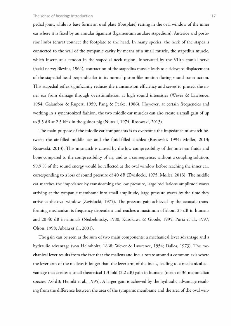
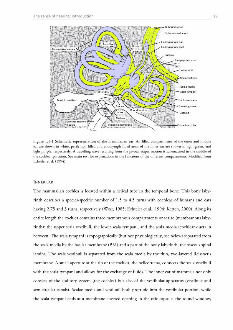
The middle ear is an air filled pouch, the tympanic cavity (cavum tympani), that contains a se-
ries of functionally interconnected membranes and three small bones (malleus, incus, stapes), that
couple the incoming sound stimulus to the inner ear (Figure 1.1-1). In many mammals the tym-
panic cavity is ventrally extended and protrudes from the skull base as an oval shaped knob, then
called bulla tympanica (Keen & Grobbelaar, 1941). The most lateral part of the middle ear is the
The sense of hearing: Introduction 16
tympanic membrane, a thin cone-shaped membrane stretched within a bony tympanic ring at the
medial end of the ear canal. The mammalian tympanic membrane consists of two components, a
thinner and stiffer pars tensa and a loose pars flaccida, the size of which is highly variable between
different species (Kohllöffel, 1984; Vrettakos et al., 1988). The function of the pars flaccida is still
subject of ongoing discussions, but it probably influences low frequency sensitivity and ensures
static pressure consistency on both sides of the tympanic membrane (Hellström & Stenfors,
1983; Kohllöffel, 1984; Rosowski, 2010; Rosowski, 2013). The pars tensa is the first station of
the middle ear acoustic transduction chain and is directly coupled to the first of the three bones
of the ossicular chain within the mammalian middle ear: the malleus.
The malleus, the largest of the three ossicles, adheres to the centre of the pars tensa (umbo) of
the tympanic membrane via a long handle, the manubrium; the contact surface of this attach-
ment differs between species: some show only local adherence while in others the whole manu-
brium is attached to the tympanic membrane along its entire length (Rosowski, 2010). The op-
posite end of the malleus, the head (caput), features a saddle-shaped surface which serves as a facet
joint to the incus, the next ossicle in the chain (a flexible joint is the case in most species; in many
rodents, however, the two bones are partly or completely fused; Fleischer, 1973). The region be-
tween manubrium and caput of the malleus is called the neck (collum). Two processes emerge
from the malleus at the junction between the neck and the handle: a larger lateral process con-
nected to the tympanic membrane and a shorter anterior process connected to the wall of the
tympanic cavity by the anterior mallear ligament. The musculus tensor tympani inserts at the ba-
sal region of the manubrium and pulls it inwards when contracted. It is innervated by the motor
branch of the trigeminal nerve (Møller, 2013).
The incus has approximately the shape of an anvil with a saddle, the incudomallear joint, po-
sitioned on the face. The longer of the two arms, crus longum, is oriented nearly vertically
downwards but describes a sharp turn at its end and medially terminates in a small oval plate, the
processus lenticularis, which, as part of the incudostapedial joint, connects the incus to the stapes.
The shorter process of the incus, crus breve, is thicker than the crus longum and serves as an at-
tachment for the posterior ligament of the middle ear, that fixes the incus within a small depres-
sion of the epitympanum, the fossa incudis.
The stapes is by far the smallest and most fragile of the three ossicles and bears close resem-
blance to a stirrup. The top (head and neck) of the stapes forms the medial part of the incudosta-
The sense of hearing: Introduction 17
pedial joint, while its base forms an oval plate (footplate) resting in the oval window of the inner
ear where it is fixed by an annular ligament (ligamentum anulare stapedium). Anterior and poste-
rior limbs (crura) connect the footplate to the head. In many species, the neck of the stapes is
connected to the wall of the tympanic cavity by means of a small muscle, the stapedius muscle,
which inserts at a tendon in the stapedial neck region. Innervated by the VIIth cranial nerve
(facial nerve; Blevins, 1964), contraction of the stapedius muscle leads to a sideward displacement
of the stapedial head perpendicular to its normal piston-like motion during sound transduction.
This stapedial reflex significantly reduces the transmission efficiency and serves to protect the in-
ner ear from damage through overstimulation at high sound intensities (Wever & Lawrence,
1954; Galambos & Rupert, 1959; Pang & Peake, 1986). However, at certain frequencies and
working in a synchronized fashion, the two middle ear muscles can also create a small gain of up
to 5.5 dB at 2.5 kHz in the guinea pig (Nuttall, 1974; Rosowski, 2013).
The main purpose of the middle ear components is to overcome the impedance mismatch be-
tween the air-filled middle ear and the fluid-filled cochlea (Rosowski, 1994; Møller, 2013;
Rosowski, 2013). This mismatch is caused by the low compressibility of the inner ear fluids and
bone compared to the compressibility of air, and as a consequence, without a coupling solution,
99.9 % of the sound energy would be reflected at the oval window before reaching the inner ear,
corresponding to a loss of sound pressure of 40 dB (Zwislocki, 1975; Møller, 2013). The middle
ear matches the impedance by transforming the low pressure, large oscillations amplitude waves
arriving at the tympanic membrane into small amplitude, large pressure waves by the time they
arrive at the oval window (Zwislocki, 1975). The pressure gain achieved by the acoustic trans-
forming mechanism is frequency dependent and reaches a maximum of about 25 dB in humans
and 20-40 dB in animals (Nedzelnitsky, 1980; Kurokawa & Goode, 1995; Puria et al., 1997;
Olson, 1998; Aibara et al., 2001).
The gain can be seen as the sum of two main components: a mechanical lever advantage and a
hydraulic advantage (von Helmholtz, 1868; Wever & Lawrence, 1954; Dallos, 1973). The me-
chanical lever results from the fact that the malleus and incus rotate around a common axis where
the lever arm of the malleus is longer than the lever arm of the incus, leading to a mechanical ad-
vantage that creates a small theoretical 1.3 fold (2.2 dB) gain in humans (mean of 36 mammalian
species: 7.6 dB; Hemilä et al., 1995). A larger gain is achieved by the hydraulic advantage result-
ing from the difference between the area of the tympanic membrane and the area of the oval win-
The sense of hearing: Introduction 18
dow. In humans, this area ratio is 20:1, leading to a theoretical amplification of additional 26 dB
(mean of 36 mammalian species: 29 dB; Hemilä et al., 1995). Helmholtz (1863) originally pro-
posed a third amplifying mechanism operating at the tympanic membrane: the buckling move-
ment resulting from the conical suspension of the tympanic membrane could act as a catenary
lever, yielding approximately 6 dB gain in humans. The results of extensive studies by Wever and
Lawrence (1954) and Békésy and Wever (1960) initially did not corroborate the tympanic cate-
nary lever, but more recent measurements and models of sound-induced tympanic membrane
surface motions are in line with the catenary lever mechanism (Tonndorf & Khanna, 1970,
1972; Khanna & Tonndorf, 1972; Funnell et al., 1987; Fay et al., 2006). Taking the catenary
lever into account, all means of amplification yield a total theoretical human middle ear gain of
34 dB. This value is lower than expected for an ideal transformer (40 dB) and much larger than
what was actually measured in mammalian middle ears. The difference between the theoretical
and actually measured gain can be explained by losses through ossicular elasticity (Funnell et al.,
1992; Decraemer et al., 1995), flexion in the ossicular joints (Guinan & Peake, 1967; Willi et al.,
2002; Funnell et al., 2005), complicated irregular translational and rotational motions of malleus
and incus at high frequencies (Decraemer & Khanna, 2004), and alterations in the stiffness and
effective area of the tympanic membrane (Fay et al., 2006; Rosowski, 2010), all of which are fre-
quency dependent factors that are hard to take into account in simple models. It is evident that
the middle ear does not act as an ideal transformer (Rosowski, 1991) but it is efficient enough to
transfer information about biologically relevant acoustic signals to the inner ear.
The sense of hearing: Introduction 19
Figure 1.1-1 Schematic representation of the mammalian ear. Air filled compartments of the outer and middle ear are shown in white, perilymph filled and endolymph filled areas of the inner ear are shown in light green, and light purple, respectively. A travelling wave resulting from the pivotal stapes motion is schematized in the middle of the cochlear partition. See main text for explanations in the functions of the different compartments. Modified from Echteler et al. (1994).
INNER EAR
The mammalian cochlea is located within a helical tube in the temporal bone. This bony laby-
rinth describes a species-specific number of 1.5 to 4.5 turns with cochleae of humans and cats
having 2.75 and 3 turns, respectively (West, 1985; Echteler et al., 1994; Ketten, 2000). Along its
entire length the cochlea contains three membranous compartments or scalae (membranous laby-
rinth): the upper scala vestibuli, the lower scala tympani, and the scala media (cochlear duct) in
between. The scala tympani is topographically (but not physiologically, see below) separated from
the scala media by the basilar membrane (BM) and a part of the bony labyrinth, the osseous spiral
lamina. The scala vestibuli is separated from the scala media by the thin, two-layered Reissner’s
membrane. A small aperture at the tip of the cochlea, the helicotrema, connects the scala vestibuli
with the scala tympani and allows for the exchange of fluids. The inner ear of mammals not only
consists of the auditory system (the cochlea) but also of the vestibular apparatus (vestibule and
semicircular canals). Scalae media and vestibuli both protrude into the vestibular portion, while
the scala tympani ends at a membrane-covered opening in the otic capsule, the round window,
The sense of hearing: Introduction 20
facing the air filled middle ear. As already mentioned above, the oval window, holds the footplate
of the stapes and faces the basal scala vestibuli (overview in Figure 1.1-1).
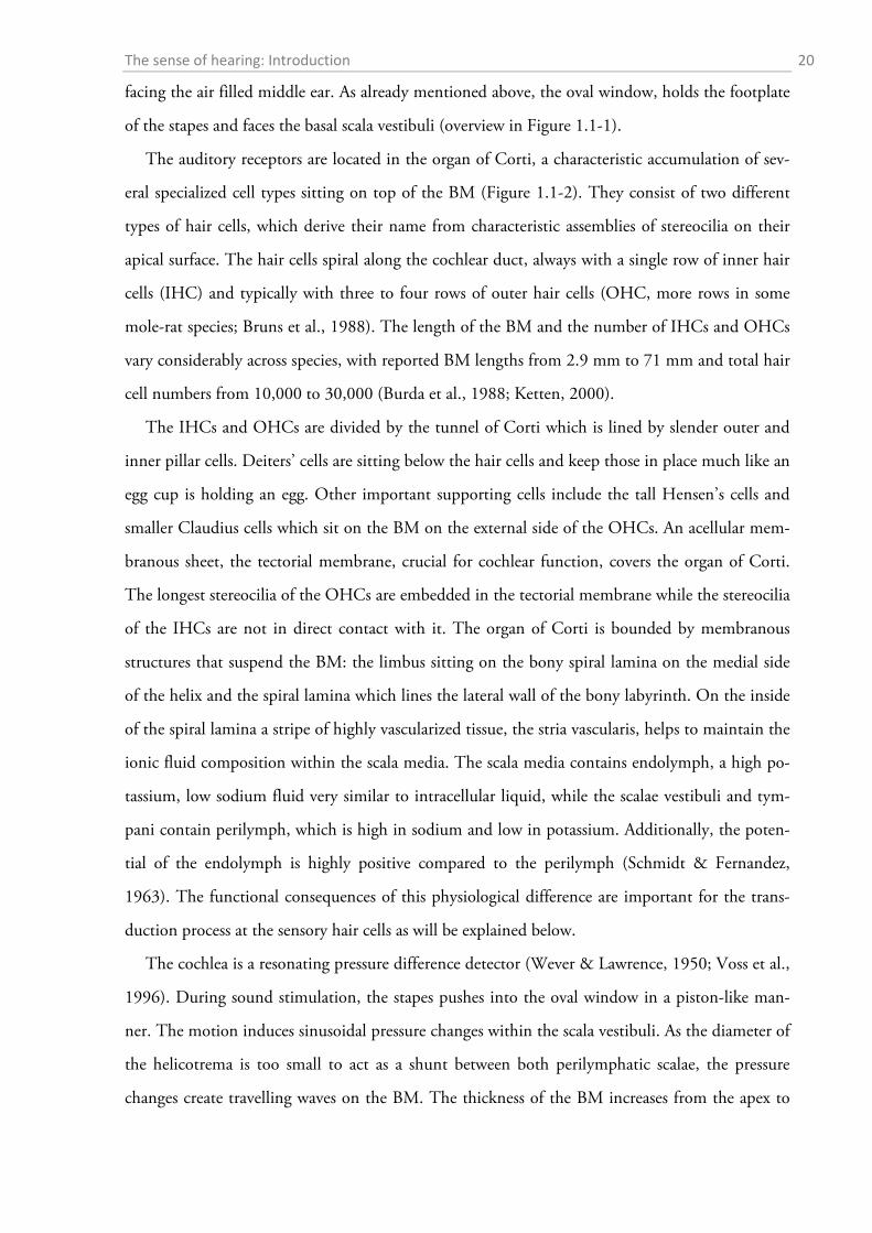
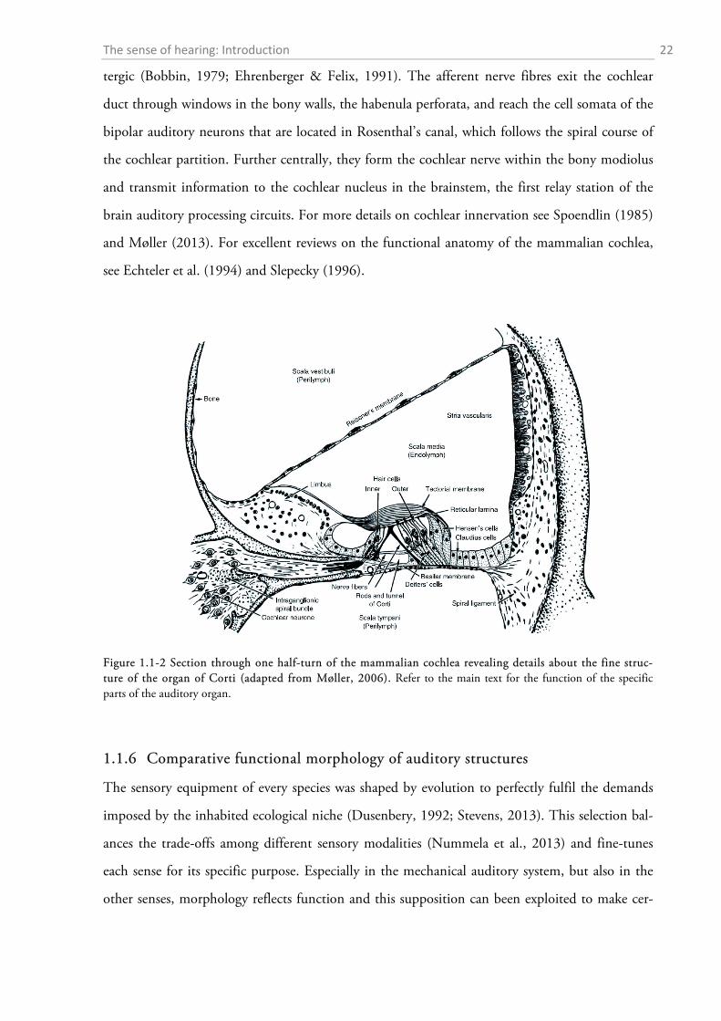
The auditory receptors are located in the organ of Corti, a characteristic accumulation of sev-
eral specialized cell types sitting on top of the BM (Figure 1.1-2). They consist of two different
types of hair cells, which derive their name from characteristic assemblies of stereocilia on their
apical surface. The hair cells spiral along the cochlear duct, always with a single row of inner hair
cells (IHC) and typically with three to four rows of outer hair cells (OHC, more rows in some
mole-rat species; Bruns et al., 1988). The length of the BM and the number of IHCs and OHCs
vary considerably across species, with reported BM lengths from 2.9 mm to 71 mm and total hair
cell numbers from 10,000 to 30,000 (Burda et al., 1988; Ketten, 2000).
The IHCs and OHCs are divided by the tunnel of Corti which is lined by slender outer and
inner pillar cells. Deiters’ cells are sitting below the hair cells and keep those in place much like an
egg cup is holding an egg. Other important supporting cells include the tall Hensen’s cells and
smaller Claudius cells which sit on the BM on the external side of the OHCs. An acellular mem-
branous sheet, the tectorial membrane, crucial for cochlear function, covers the organ of Corti.
The longest stereocilia of the OHCs are embedded in the tectorial membrane while the stereocilia
of the IHCs are not in direct contact with it. The organ of Corti is bounded by membranous
structures that suspend the BM: the limbus sitting on the bony spiral lamina on the medial side
of the helix and the spiral lamina which lines the lateral wall of the bony labyrinth. On the inside
of the spiral lamina a stripe of highly vascularized tissue, the stria vascularis, helps to maintain the
ionic fluid composition within the scala media. The scala media contains endolymph, a high po-
tassium, low sodium fluid very similar to intracellular liquid, while the scalae vestibuli and tym-
pani contain perilymph, which is high in sodium and low in potassium. Additionally, the poten-
tial of the endolymph is highly positive compared to the perilymph (Schmidt & Fernandez,
1963). The functional consequences of this physiological difference are important for the trans-
duction process at the sensory hair cells as will be explained below.
The cochlea is a resonating pressure difference detector (Wever & Lawrence, 1950; Voss et al.,
1996). During sound stimulation, the stapes pushes into the oval window in a piston-like man-
ner. The motion induces sinusoidal pressure changes within the scala vestibuli. As the diameter of
the helicotrema is too small to act as a shunt between both perilymphatic scalae, the pressure
changes create travelling waves on the BM. The thickness of the BM increases from the apex to
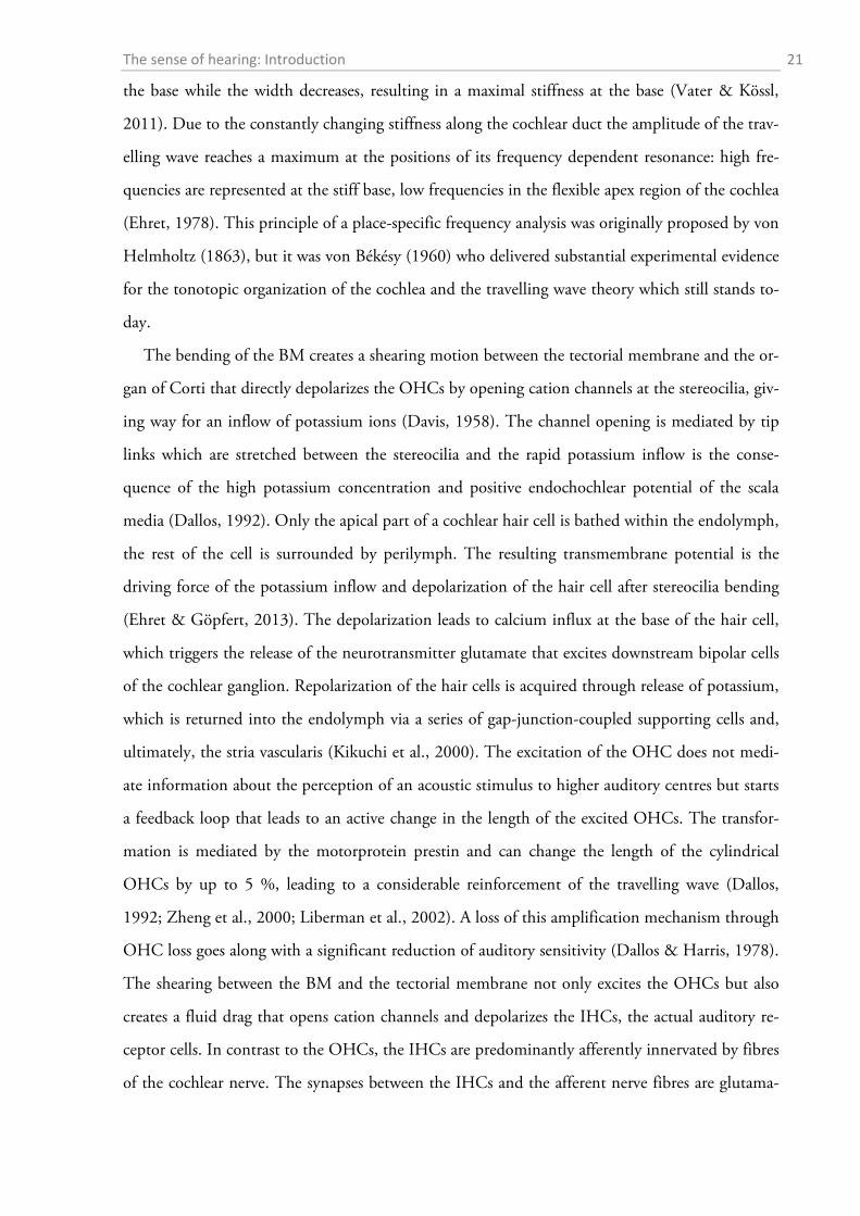
The sense of hearing: Introduction 21
the base while the width decreases, resulting in a maximal stiffness at the base (Vater & Kössl,
2011). Due to the constantly changing stiffness along the cochlear duct the amplitude of the trav-
elling wave reaches a maximum at the positions of its frequency dependent resonance: high fre-
quencies are represented at the stiff base, low frequencies in the flexible apex region of the cochlea
(Ehret, 1978). This principle of a place-specific frequency analysis was originally proposed by von
Helmholtz (1863), but it was von Békésy (1960) who delivered substantial experimental evidence
for the tonotopic organization of the cochlea and the travelling wave theory which still stands to-
day.
The bending of the BM creates a shearing motion between the tectorial membrane and the or-
gan of Corti that directly depolarizes the OHCs by opening cation channels at the stereocilia, giv-
ing way for an inflow of potassium ions (Davis, 1958). The channel opening is mediated by tip
links which are stretched between the stereocilia and the rapid potassium inflow is the conse-
quence of the high potassium concentration and positive endochochlear potential of the scala
media (Dallos, 1992). Only the apical part of a cochlear hair cell is bathed within the endolymph,
the rest of the cell is surrounded by perilymph. The resulting transmembrane potential is the
driving force of the potassium inflow and depolarization of the hair cell after stereocilia bending
(Ehret & Göpfert, 2013). The depolarization leads to calcium influx at the base of the hair cell,
which triggers the release of the neurotransmitter glutamate that excites downstream bipolar cells
of the cochlear ganglion. Repolarization of the hair cells is acquired through release of potassium,
which is returned into the endolymph via a series of gap-junction-coupled supporting cells and,
ultimately, the stria vascularis (Kikuchi et al., 2000). The excitation of the OHC does not medi-
ate information about the perception of an acoustic stimulus to higher auditory centres but starts
a feedback loop that leads to an active change in the length of the excited OHCs. The transfor-
mation is mediated by the motorprotein prestin and can change the length of the cylindrical
OHCs by up to 5 %, leading to a considerable reinforcement of the travelling wave (Dallos,
1992; Zheng et al., 2000; Liberman et al., 2002). A loss of this amplification mechanism through
OHC loss goes along with a significant reduction of auditory sensitivity (Dallos & Harris, 1978).
The shearing between the BM and the tectorial membrane not only excites the OHCs but also
creates a fluid drag that opens cation channels and depolarizes the IHCs, the actual auditory re-
ceptor cells. In contrast to the OHCs, the IHCs are predominantly afferently innervated by fibres
of the cochlear nerve. The synapses between the IHCs and the afferent nerve fibres are glutama-
The sense of hearing: Introduction 22
tergic (Bobbin, 1979; Ehrenberger & Felix, 1991). The afferent nerve fibres exit the cochlear
duct through windows in the bony walls, the habenula perforata, and reach the cell somata of the
bipolar auditory neurons that are located in Rosenthal’s canal, which follows the spiral course of
the cochlear partition. Further centrally, they form the cochlear nerve within the bony modiolus
and transmit information to the cochlear nucleus in the brainstem, the first relay station of the
brain auditory processing circuits. For more details on cochlear innervation see Spoendlin (1985)
and Møller (2013). For excellent reviews on the functional anatomy of the mammalian cochlea,
see Echteler et al. (1994) and Slepecky (1996).
Figure 1.1-2 Section through one half-turn of the mammalian cochlea revealing details about the fine struc-ture of the organ of Corti (adapted from Møller, 2006). Refer to the main text for the function of the specific parts of the auditory organ.
1.1.6 Comparative functional morphology of auditory structures
The sensory equipment of every species was shaped by evolution to perfectly fulfil the demands
imposed by the inhabited ecological niche (Dusenbery, 1992; Stevens, 2013). This selection bal-
ances the trade-offs among different sensory modalities (Nummela et al., 2013) and fine-tunes
each sense for its specific purpose. Especially in the mechanical auditory system, but also in the
other senses, morphology reflects function and this supposition can been exploited to make cer-
The sense of hearing: Introduction 23
tain predictions about the hearing capabilities of inaccessible or even extinct species on the basis
of anatomical data alone (e.g. Rosowski & Graybeal, 1991).
From the functional description of the outer and middle ear given above, one might suppose
that it is relatively easy to straightforwardly predict the auditory sensitivity of a mammal species
by simply calculating the total impedance transformation efficiency, which is quickly done by
summing up the gain of each component (lever arm ratio, area ratio, possibly tympanic mem-
brane lever advantage). Following this simple logic, the efficiency of every mammalian middle ear
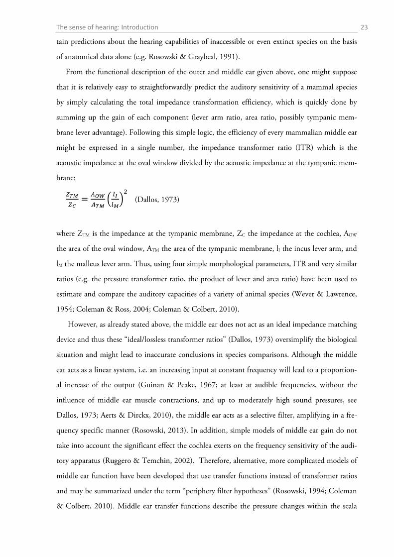
might be expressed in a single number, the impedance transformer ratio (ITR) which is the
acoustic impedance at the oval window divided by the acoustic impedance at the tympanic mem-
brane:
𝑍𝑇𝑇𝑍𝐶
= 𝐴𝑂𝑂𝐴𝑇𝑇
� 𝑙𝐼𝑙𝑇�2 (Dallos, 1973)
where ZTM is the impedance at the tympanic membrane, ZC the impedance at the cochlea, AOW
the area of the oval window, ATM the area of the tympanic membrane, lI the incus lever arm, and
lM the malleus lever arm. Thus, using four simple morphological parameters, ITR and very similar
ratios (e.g. the pressure transformer ratio, the product of lever and area ratio) have been used to
estimate and compare the auditory capacities of a variety of animal species (Wever & Lawrence,
1954; Coleman & Ross, 2004; Coleman & Colbert, 2010).
However, as already stated above, the middle ear does not act as an ideal impedance matching
device and thus these “ideal/lossless transformer ratios” (Dallos, 1973) oversimplify the biological
situation and might lead to inaccurate conclusions in species comparisons. Although the middle
ear acts as a linear system, i.e. an increasing input at constant frequency will lead to a proportion-
al increase of the output (Guinan & Peake, 1967; at least at audible frequencies, without the
influence of middle ear muscle contractions, and up to moderately high sound pressures, see
Dallos, 1973; Aerts & Dirckx, 2010), the middle ear acts as a selective filter, amplifying in a fre-
quency specific manner (Rosowski, 2013). In addition, simple models of middle ear gain do not
take into account the significant effect the cochlea exerts on the frequency sensitivity of the audi-
tory apparatus (Ruggero & Temchin, 2002). Therefore, alternative, more complicated models of
middle ear function have been developed that use transfer functions instead of transformer ratios
and may be summarized under the term “periphery filter hypotheses” (Rosowski, 1994; Coleman
& Colbert, 2010). Middle ear transfer functions describe the pressure changes within the scala
The sense of hearing: Introduction 24
vestibuli or the velocity of the stapes in dependence of the sound pressure reaching the tympanic
membrane for a broad range of frequencies and thus perfectly describe the frequency dependence
of the middle ear system and the cochlear impedance (see below). The functions correlate well
with the shape of behavioural audiograms (Dallos, 1973; Zwislocki, 1975; Ehret & Göpfert,
2013). However, obtaining transfer functions is a complicated and invasive procedure that has so
far mainly been used on standard laboratory animals such as cat and guinea pig (Møller, 1963;
Décory et al., 1990). Because transfer functions obtained from cadavers differ considerably from
those measured in vivo (Ruggero & Temchin, 2003), such measurements are almost impossible
to get from most wild mammal species. As it is unclear to what extent the transfer functions ob-
tained in laboratory species apply to the ears of other mammalian species, to determine the audi-
tory capacities of these species, we are left with correlation-based models and time consuming be-
havioural experiments.
Several morphological parameters of the mammalian outer, middle and inner ear correlate well
with certain characteristics of behavioural audiograms, as was revealed by studies employing a
simple approach: collecting a number of morphological parameters of species with known audio-
grams or neurophysiological investigations and test for correlations between both parameters (e.g.
Rosowski, 1992; Echteler et al., 1994; Vater & Kössl, 2011). Strong correlations have been found
and the regression lines can be used to predict the sensitivity of auditory structures. The parame-
ters comprise the whole morphological spectrum including the number of turns of the cochlea
(West, 1985), the weight and dimensions of the middle ear ossicles (Hemilä et al., 1995), the
length, width, and stiffness of the BM (Vater & Kössl, 2011), the length of the hair cells
(Dannhof et al., 1991), as well as the shape of the outer ear (Coleman & Ross, 2004; Coleman &
Colbert, 2010). The revealed correlations are of highly variable strength and often heavily de-
pendent on the chosen data set, but in general, a unified understanding of the relationship be-
tween mammalian ear diversity and hearing seems in reach. It is necessary to increase the dataset
of mammalian species for which parameters of both, auditory morphology and hearing capabili-
ties, are covered in detail to create or refine models of mammalian ear function. This will also re-
veal differences between the fits of different models and allow for the right choice. Hopefully one
day, a simple, correctly chosen model will allow highly accurate predictions of hearing capabilities
in extinct and hard to study mammals.
The sense of hearing: Material & Methods 25
1.2 Material and Methods
1.2.1 Behavioural audiometry
SUBJECTS
Three young (3-8 month old) red foxes (Vulpes vulpes, two males and one female) were tested.
The experiments were performed in an empty horse stable in a rural area of the Bohemian Forest,
Czech Republic (49°9'10.28"N, 13°20'56.45"E). The animals were kept in cages outdoors or
within the stable by foresters as pets with permits of the local veterinary medical and Nature and
Animal Protection authorities. The daily acoustic environment of the animals consisted mainly of
natural environmental sounds and some occasional noise of cars infrequently passing on a nearby
small road. The foxes were fed on dry canine diet and were given access to water ad libitum. The
foxes received at least 80% of their daily food ration during the training and test sessions. Daily
monitoring ensured the good health of the animals. One animal (female) was trained and tested
in 2012, two other animals in 2013. In addition, one human subject (male, 28 years old) was
tested with the same equipment and at the same location.
SETUP
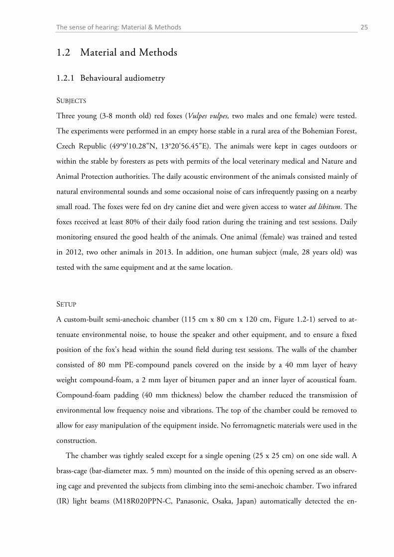
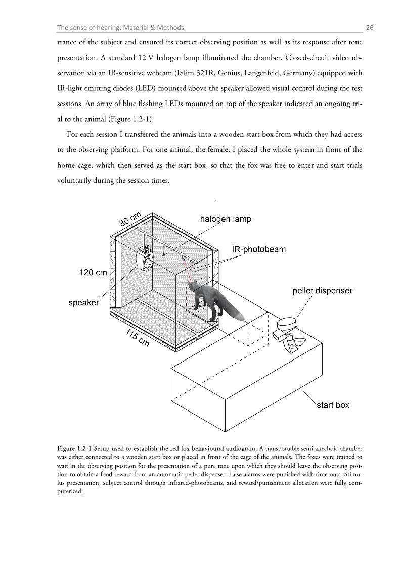
A custom-built semi-anechoic chamber (115 cm x 80 cm x 120 cm, Figure 1.2-1) served to at-
tenuate environmental noise, to house the speaker and other equipment, and to ensure a fixed
position of the fox’s head within the sound field during test sessions. The walls of the chamber
consisted of 80 mm PE-compound panels covered on the inside by a 40 mm layer of heavy
weight compound-foam, a 2 mm layer of bitumen paper and an inner layer of acoustical foam.
Compound-foam padding (40 mm thickness) below the chamber reduced the transmission of
environmental low frequency noise and vibrations. The top of the chamber could be removed to
allow for easy manipulation of the equipment inside. No ferromagnetic materials were used in the
construction.
The chamber was tightly sealed except for a single opening (25 x 25 cm) on one side wall. A
brass-cage (bar-diameter max. 5 mm) mounted on the inside of this opening served as an observ-
ing cage and prevented the subjects from climbing into the semi-anechoic chamber. Two infrared
(IR) light beams (M18R020PPN-C, Panasonic, Osaka, Japan) automatically detected the en-
The sense of hearing: Material & Methods 26
trance of the subject and ensured its correct observing position as well as its response after tone
presentation. A standard 12 V halogen lamp illuminated the chamber. Closed-circuit video ob-
servation via an IR-sensitive webcam (ISlim 321R, Genius, Langenfeld, Germany) equipped with
IR-light emitting diodes (LED) mounted above the speaker allowed visual control during the test
sessions. An array of blue flashing LEDs mounted on top of the speaker indicated an ongoing tri-
al to the animal (Figure 1.2-1).
For each session I transferred the animals into a wooden start box from which they had access
to the observing platform. For one animal, the female, I placed the whole system in front of the
home cage, which then served as the start box, so that the fox was free to enter and start trials
voluntarily during the session times.
Figure 1.2-1 Setup used to establish the red fox behavioural audiogram. A transportable semi-anechoic chamber was either connected to a wooden start box or placed in front of the cage of the animals. The foxes were trained to wait in the observing position for the presentation of a pure tone upon which they should leave the observing posi-tion to obtain a food reward from an automatic pellet dispenser. False alarms were punished with time-outs. Stimu-lus presentation, subject control through infrared-photobeams, and reward/punishment allocation were fully com-puterized.
The sense of hearing: Material & Methods 27
STIMULUS CONTROL
I used a multi-I/O processor unit (RZ6, Tucker-Davis Technologies (TDT), Alachua, FL, USA)
with a maximal sampling rate of 200 kHz to generate, amplify and attenuate pure tones of
500 ms duration. A software-controlled cosine gate (RPvdsEx V. 74, TDT) created rise and fall
times of 25 ms and 50 ms for frequencies above 63 Hz and up to 63 Hz, respectively. Stimuli
with frequencies higher than 63 Hz were transmitted through a dual concentric loudspeaker
(Arena Satellite, Tannoy, UK; 80 Hz-54 kHz frequency response), for the frequencies 50 Hz and
63 Hz I used a 12” (30 cm) subwoofer (Punch HE, Rockford Fosgate, Tempe, AZ, USA; 28-200
Hz frequency response). The dual concentric loudspeaker was mounted at 0° elevation and at a
distance of 60 cm in front of the animal while the subwoofer was placed on the foam-covered
floor of the chamber with the speaker membrane facing away from the animal.
I calibrated the sound intensity at the head position for each frequency at 80 dB sound pres-
sure level (SPL, re 20 µPa) with a Precision Sound Level Meter (2231, Brüel & Kjær (B&K),
Naerum, Denmark) equipped with a 1/4” free field microphone (4939, B&K, 4 Hz-100 kHz;
corrected for free field response with protection grid on). The sound level meter was calibrated
before each measurement with a sound level calibrator (4230, B&K; 94 dB re 20 µPa at 1 kHz)
equipped with a 1/4” adaptor (DP-0775, B&K). A flexible extension rod (UA-0196, B&K) min-
imized the risk of measuring reflections from the 2231 case. I used an 1/3-octave filterset (1625,
B&K) to measure sound pressure levels between 50 Hz and 20 kHz, for higher frequencies I
measured with the high pass (>12.5 kHz) filter of an infra- and ultrasound filter set (1627,
B&K). For all sound measurements I used linear frequency weighting. Because the head of the
animal was not fixed within the sound field I controlled the presented sound intensities as fol-
lows. At each frequency I assessed three SPL values within the observing cage: SPL at the observ-
ing position (dBob), maximum SPL (dBmax) and minimum SPL (dBmin). I then took care to meet
the following two criteria during calibration. First, the maximal value at any point within the ob-
serving cage was not higher than + 2 dB SPL above the desired intensity (dSPL). Second, the dif-
ference between dSPL and the mean (dBmin, dBmax) was smaller than 6 dB. This procedure resulted
in homogeneity of the presented sound field of ± 3 dB. Eventually, since most deviations oc-
curred in the corners of the observing cage which were rarely visited by the animal, the actual
sound field experienced by the animal was even more homogenous. To control the sound stimuli
for harmonics and distortion I connected the output of the sound level meter to a digital USB
The sense of hearing: Material & Methods 28
oscilloscope (PicoScope 4224, Pico Technology, Cambridgeshire, UK) and employed the fre-
quency analyzing FFT-function of the corresponding software (PicoScope 6, Pico Technology).
I determined the ambient noise levels with the same devices that were used to calibrate the
stimulus intensity. To assess the attenuation properties of the semi-anechoic chamber I recorded
the noise intensities alternately on the inside and outside of the chamber shortly before or after a
test session over a period of 10 days. I did not perform these measurements during the experi-
mental procedure since noise created by movement of the experimental animals would have dis-
torted the measurements which were intended to reflect the background noise during the periods
of silent listening. For measurements inside of the chamber I inserted the microphone into the
chamber through the cable passage at the back (confer Figure 1.2-1). For outside measurements I
alternately placed the microphone either on the left or right side of the chamber. I took a single
SPL reading in each of 31 1/3-octave bandwidth windows with centre frequencies between 20 Hz
and 20 kHz. In addition, I measured ambient noise SPL in the low- (< 20 Hz) and high frequen-
cy (> 12.5 kHz-100 kHz) range using the respective filter settings (B&K 1627). It took about 15
min per session to accomplish all ambient noise measurements. Due to the low levels of the am-
bient noise which were at the lower end of the sensitivity range of the sound level meter, I later
corrected the measurements for the internal noise level of the microphone amplifier combination
according to the specifications of Brüel & Kjær to avoid overestimations of the noise (personal
communication with Ralf Klaerner, B&K).
PSYCHOPHYSICAL PROCEDURE
I employed a simple go/no-go procedure. I trained the foxes to enter the chamber through a win-
dow which automatically started a trial and required the animals to wait in a observing position
until a tone was presented. Upon tone perception the foxes should leave the observing position to
indicate the detection of the stimulus. Correct responses were automatically rewarded with dry
dog kibbles delivered directly into the starting box (or home cage for the female) by an electronic
pellet dispenser (ENV-203-190 mg, Med associates Inc, St Albans, VT, USA) which was custom-
ized to accommodate ordinary dry dog kibbles (Adult Mini, Interquell Happy Dog, Großait-
ingen, Germany). Punishment was given in form of time-outs during which the foxes had to wait
before a new trial could be initiated which were indicated by switched-off chamber lighting.
The sense of hearing: Material & Methods 29
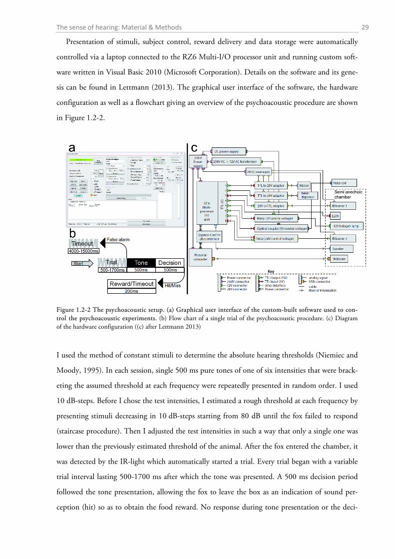
Presentation of stimuli, subject control, reward delivery and data storage were automatically
controlled via a laptop connected to the RZ6 Multi-I/O processor unit and running custom soft-
ware written in Visual Basic 2010 (Microsoft Corporation). Details on the software and its gene-
sis can be found in Lettmann (2013). The graphical user interface of the software, the hardware
configuration as well as a flowchart giving an overview of the psychoacoustic procedure are shown
in Figure 1.2-2.
Figure 1.2-2 The psychoacoustic setup. (a) Graphical user interface of the custom-built software used to con-trol the psychoacoustic experiments. (b) Flow chart of a single trial of the psychoacoustic procedure. (c) Diagram of the hardware configuration ((c) after Lettmann 2013)
I used the method of constant stimuli to determine the absolute hearing thresholds (Niemiec and
Moody, 1995). In each session, single 500 ms pure tones of one of six intensities that were brack-
eting the assumed threshold at each frequency were repeatedly presented in random order. I used
10 dB-steps. Before I chose the test intensities, I estimated a rough threshold at each frequency by
presenting stimuli decreasing in 10 dB-steps starting from 80 dB until the fox failed to respond
(staircase procedure). Then I adjusted the test intensities in such a way that only a single one was
lower than the previously estimated threshold of the animal. After the fox entered the chamber, it
was detected by the IR-light which automatically started a trial. Every trial began with a variable
trial interval lasting 500-1700 ms after which the tone was presented. A 500 ms decision period
followed the tone presentation, allowing the fox to leave the box as an indication of sound per-
ception (hit) so as to obtain the food reward. No response during tone presentation or the deci-
The sense of hearing: Material & Methods 30
sion phase (miss) resulted in a short switch-off of the chamber lighting to indicate the fox to leave
the chamber before a new trial could be initiated. Responses during the trial interval or during
catch trials where no tone was presented were denoted as false alarms (FA) and followed by a
punishment interval of 4-15 s depending on the mood and character of the fox.
I tested the foxes in two to four daily sessions with each session consisting of roughly 100 trials
+ 25 catch trials. A total of 15 different frequencies from 50 Hz to 54 kHz was tested (50 Hz, 63
Hz, 125 Hz, 250 Hz, 500 Hz, 1 kHz, 2 kHz, 4 kHz, 6.3 kHz, 8 kHz, 16 kHz, 32 kHz, 40 kHz,
46 kHz, 54 kHz). To determine the threshold at each frequency, I first calculated the hit rate at
each tested intensity for each session and converted it into a performance measure which I then
corrected for false alarms (Heffner & Heffner, 1988b, 1995). I chose the performance measure:
performance = hit rate – (hit rate x FA rate), resulting in values between 0 and 1 (with 1 meaning
100% hit rate and no FA; Heffner & Heffner, 1988b). Plotting the performance in each session
against the intensity yielded a psychometric function where I calculated the threshold at the test-
ed frequency through interpolation of the intensity where the performance reached a level of 0.5.
The final threshold of each animal and frequency was then the mean of the first three sessions
that satisfied the following stability criterion: each of the three thresholds lay within ± 5 dB of
their respective mean. I discarded test sessions with FA rates higher than 25 %.
1.2.2 Morphometric analysis of the outer and middle ear
The aim of the morphological description of the red fox ear was to reveal correlations between
morphometric parameters and properties of the behavioural audiogram, which would ultimately
allow for a precise estimation of auditory sensitivity on the basis of morphological data alone.
Therefore, the analysis was restricted to the parts of the ear involved in auditory function. I used
fresh tissue that was obtained by hunters in the Czech Republic which were instructed and super-
vised by Dr. Ing. Vlastimil Hart and Prof. Dr. Ing. Jaroslav Červený, Department of Game Man-
agement and Wildlife Biology, Faculty of Forestry and Wood Sciences, Czech University of Life
Sciences, Prague, Czech Republic. Additionally, I used skulls belonging to my private collection
and to the collection of the Senckenberg Museum of Natural History Görlitz (generously provid-
ed by Prof. Dr. Hermann Ansorge). All foxes were killed by licensed hunters based on regular
shooting schedules; no fox was killed or harmed specifically for this study.
The sense of hearing: Material & Methods 31
To preserve fresh tissue, the heads of freshly shot red foxes (Vulpes vulpes) were immersion
fixed by the hunters in the field in either 10 % formalin solution in water or 4 % paraformalde-
hyde (PFA)-solution in 0.1 M phosphate buffer (PB). To promote tissue penetration, the fixative
was also injected into the ear canal, the muscles surrounding the bulla tympanica, and the eyes for
optimal fixation of the retina. The time of fixation of the heads differed between the individuals
and ranged from a minimum of two weeks to several years for old specimens from the archive of
the Department of General Zoology, University of Duisburg-Essen.
Before preparation of the middle and inner ear the heads were rinsed for several hours with tap
water. The eyes were carefully removed with titanium forceps and ceramic scalpels (World preci-
sion instruments (WPI), Berlin, Germany) and stored in phosphate buffered saline (PBS, with
0.05 % sodium azide added as a preservative) at 4 °C or for later analysis. Skulls from the collec-
tions had been prepared according to standard museum procedures (Mooney et al., 1982). Brief-
ly, the heads were boiled in water with added detergent for several hours after which the soft tis-
sues were easily ablated from the bones. To get a pale finish, the skulls were in most cases
bleached for 1-2 minutes in 10 % hydrogen peroxide. The procedure very often left the middle
ear ossicles in place and had no significant impact on the ossicle mass or measurements
(Nummela, 1995). The ossicles were gathered by opening of the bulla tympanica and removal
with a pair of fine forceps.
The total sample comprised material from 54 red foxes (23 fixed individuals and 31 skulls; cf.
Tables A1-A8 in the appendix for details on the individuals and the data obtained from them).
OUTER EAR AND BULLA TYMPANICA
I measured the dimensions of the pinnae with a standard ruler. In order to obtain a height to
width ratio (Coleman & Colbert, 2010), I determined the maximal width and height of each ear.
The fur, skin and mastoid muscles were removed from the skull and the lower jaw was ablated.
The bullae tympani were removed with a pair of pincers and the diameter of the proximal end of
acoustic meatus was determined with a digital calliper.
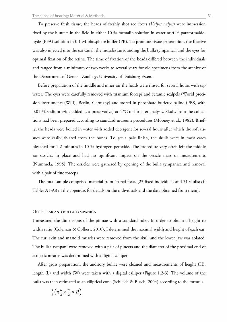
After gross preparation, the auditory bullae were cleaned and measurements of height (H),
length (L) and width (W) were taken with a digital calliper (Figure 1.2-3). The volume of the
bulla was then estimated as an elliptical cone (Schleich & Busch, 2004) according to the formula:
13�𝜋 𝐿
2× 𝑊
2× 𝐻�.
The sense of hearing: Material & Methods 32
Figure 1.2-3 Parameters that were assessed from the skull and the bulla tympanica. The drawing of the fox skull was taken from Hartová-Nentvichová et al. (2010). CBL, condylobasal length; ZGB, zygomatic breadth.
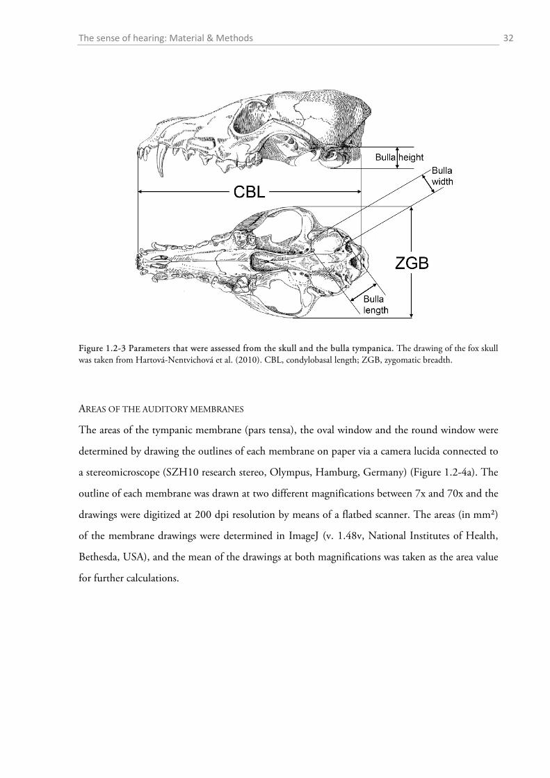
AREAS OF THE AUDITORY MEMBRANES
The areas of the tympanic membrane (pars tensa), the oval window and the round window were
determined by drawing the outlines of each membrane on paper via a camera lucida connected to
a stereomicroscope (SZH10 research stereo, Olympus, Hamburg, Germany) (Figure 1.2-4a). The
outline of each membrane was drawn at two different magnifications between 7x and 70x and the
drawings were digitized at 200 dpi resolution by means of a flatbed scanner. The areas (in mm²)
of the membrane drawings were determined in ImageJ (v. 1.48v, National Institutes of Health,
Bethesda, USA), and the mean of the drawings at both magnifications was taken as the area value
for further calculations.
The sense of hearing: Material & Methods 33
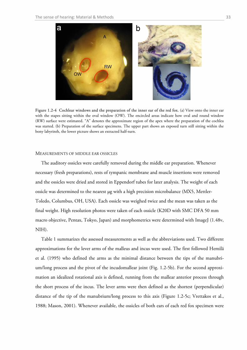
Figure 1.2-4 Cochlear windows and the preparation of the inner ear of the red fox. (a) View onto the inner ear with the stapes sitting within the oval window (OW). The encircled areas indicate how oval and round window (RW) surface were estimated. “A” denotes the approximate region of the apex where the preparation of the cochlea was started. (b) Preparation of the surface specimens. The upper part shows an exposed turn still sitting within the bony labyrinth, the lower picture shows an extracted half-turn.
MEASUREMENTS OF MIDDLE EAR OSSICLES
The auditory ossicles were carefully removed during the middle ear preparation. Whenever
necessary (fresh preparations), rests of tympanic membrane and muscle insertions were removed
and the ossicles were dried and stored in Eppendorf tubes for later analysis. The weight of each
ossicle was determined to the nearest µg with a high precision microbalance (MX5, Mettler-
Toledo, Columbus, OH, USA). Each ossicle was weighed twice and the mean was taken as the
final weight. High resolution photos were taken of each ossicle (K20D with SMC DFA 50 mm
macro objective, Pentax, Tokyo, Japan) and morphometrics were determined with ImageJ (1.48v,
NIH).
Table 1 summarizes the assessed measurements as well as the abbreviations used. Two different
approximations for the lever arms of the malleus and incus were used. The first followed Hemilä
et al. (1995) who defined the arms as the minimal distance between the tips of the manubri-
um/long process and the pivot of the incudomallear joint (Fig. 1.2-5b). For the second approxi-
mation an idealized rotational axis is defined, running from the mallear anterior process through
the short process of the incus. The lever arms were then defined as the shortest (perpendicular)
distance of the tip of the manubrium/long process to this axis (Figure 1.2-5c; Vrettakos et al.,
1988; Mason, 2001). Whenever available, the ossicles of both ears of each red fox specimen were
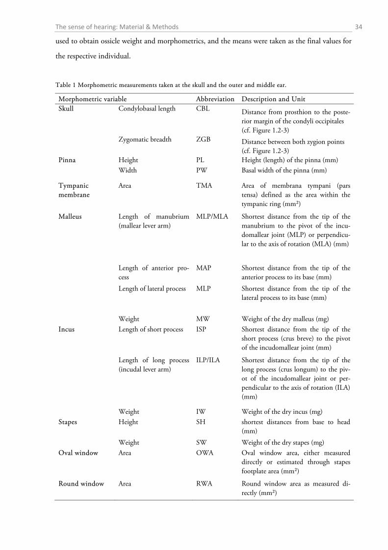
The sense of hearing: Material & Methods 34
used to obtain ossicle weight and morphometrics, and the means were taken as the final values for
the respective individual.
Table 1 Morphometric measurements taken at the skull and the outer and middle ear.
Morphometric variable Abbreviation Description and Unit Skull Condylobasal length CBL Distance from prosthion to the poste-
rior margin of the condyli occipitales (cf. Figure 1.2-3)
Zygomatic breadth ZGB Distance between both zygion points (cf. Figure 1.2-3)
Pinna Height PL Height (length) of the pinna (mm) Width PW Basal width of the pinna (mm)
Tympanic membrane
Area TMA Area of membrana tympani (pars tensa) defined as the area within the tympanic ring (mm²)
Malleus Length of manubrium (mallear lever arm)
MLP/MLA Shortest distance from the tip of the manubrium to the pivot of the incu-domallear joint (MLP) or perpendicu-lar to the axis of rotation (MLA) (mm)
Length of anterior pro-cess
MAP Shortest distance from the tip of the anterior process to its base (mm)
Length of lateral process MLP Shortest distance from the tip of the lateral process to its base (mm)
Weight MW Weight of the dry malleus (mg) Incus Length of short process ISP Shortest distance from the tip of the
short process (crus breve) to the pivot of the incudomallear joint (mm)
Length of long process (incudal lever arm)
ILP/ILA Shortest distance from the tip of the long process (crus longum) to the piv-ot of the incudomallear joint or per-pendicular to the axis of rotation (ILA) (mm)
Weight IW Weight of the dry incus (mg) Stapes Height SH shortest distances from base to head
(mm) Weight SW Weight of the dry stapes (mg) Oval window Area OWA Oval window area, either measured
directly or estimated through stapes footplate area (mm²)
Round window Area RWA Round window area as measured di-rectly (mm²)
The sense of hearing: Material & Methods 35
1.2.3 Morphometric analysis of the inner ear
The morphology of the cochlea of the red fox was analysed by means of two complementary
techniques. First, I used surface specimens to estimate sensory cell numbers and density distribu-
tions. Second, mid-modiolar microtome sections served to assess fine morpho-functional proper-
ties at different positions along the cochlear duct.
COCHLEAR WHOLE MOUNTS
To obtain whole mounts of the red fox cochlea I carefully liberated the organ of its bony encapsu-
lation with fine forceps. I prepared at a stereoscopic microscope (SZH10 research stereo, Olym-
pus) with a maximum magnification of 70x. The preparation was performed submerged in PBS
(Figure 1.2-4b). Starting in the region of the apex, I removed each half-turn, instantly stained it
with haematoxylin for one to several minutes and embedded it in glycerol on a standard micro-
scope slide. Occasional toluidine blue-staining facilitated the tissue discrimination during the
preparation process.
I analysed the stained half-turns at a light microscope (CM E, Leica, Wetzlar, Germany) at a
magnification of 1000x using an oil immersion objective. With help of an eyepiece micrometer, I
determined the densities of inner and outer hair cells as well as the width of the row of outer hair
cells (Figure 1.2-5) for each field of view over the course of the whole cochlear duct. The distance
occupied by ten (minimum of three in fields of view with extensive loss of hair cells) hair cells
served to approximate the number of hair cells per mm. By counting the number of non-
overlapping fields of view I calculated the total length of the cochlea along the tunnel of Corti,
which I then used as an estimate of the length of the basilar membrane. After counting, I assigned
all determined parameters to ten percent segments relative to the length of the basilar membrane
of the respective individual in order to allow for inter-individual analysis.
I prepared a total of eleven cochleae (seven left ears, four right ears) belonging to eight differ-
ent animals and counted the hair cells of ten of these surface specimens (the eleventh cochlea
showed severe disease related hair cell degeneration which made it impossible to count, but the
length of the basilar membrane could still be derived from this specimen). For the animals where
both ears where counted (n = 2) I included the mean of both cochleae for each position on the
basilar membrane into the final analysis.
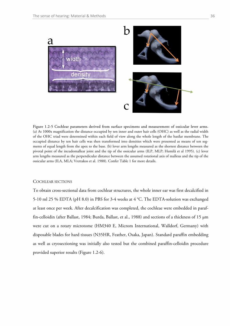
The sense of hearing: Material & Methods 36
Figure 1.2-5 Cochlear parameters derived from surface specimens and measurement of ossicular lever arms. (a) At 1000x magnification the distance occupied by ten inner and outer hair cells (OHC) as well as the radial width of the OHC triad were determined within each field of view along the whole length of the basilar membrane. The occupied distance by ten hair cells was then transformed into densities which were presented as means of ten seg-ments of equal length from the apex to the base. (b) lever arm lengths measured as the shortest distance between the pivotal point of the incudomallear joint and the tip of the ossicular arms (ILP, MLP; Hemilä et al 1995). (c) lever arm lengths measured as the perpendicular distance between the assumed rotational axis of malleus and the tip of the ossicular arms (ILA, MLA; Vrettakos et al. 1988). Confer Table 1 for more details.
COCHLEAR SECTIONS
To obtain cross-sectional data from cochlear structures, the whole inner ear was first decalcified in
5-10 ml 25 % EDTA (pH 8.0) in PBS for 3-4 weeks at 4 °C. The EDTA-solution was exchanged
at least once per week. After decalcification was completed, the cochleae were embedded in paraf-
fin-celloidin (after Ballast, 1984; Burda, Ballast, et al., 1988) and sections of a thickness of 15 µm
were cut on a rotary microtome (HM340 E, Microm International, Walldorf, Germany) with
disposable blades for hard tissues (N35HR, Feather, Osaka, Japan). Standard paraffin embedding
as well as cryosectioning was initially also tested but the combined paraffin-celloidin procedure
provided superior results (Figure 1.2-6).
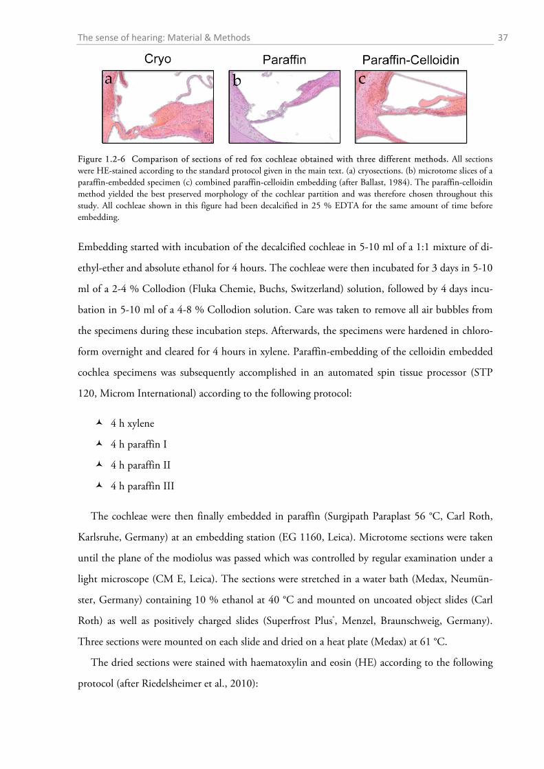
The sense of hearing: Material & Methods 37
Figure 1.2-6 Comparison of sections of red fox cochleae obtained with three different methods. All sections were HE-stained according to the standard protocol given in the main text. (a) cryosections. (b) microtome slices of a paraffin-embedded specimen (c) combined paraffin-celloidin embedding (after Ballast, 1984). The paraffin-celloidin method yielded the best preserved morphology of the cochlear partition and was therefore chosen throughout this study. All cochleae shown in this figure had been decalcified in 25 % EDTA for the same amount of time before embedding.
Embedding started with incubation of the decalcified cochleae in 5-10 ml of a 1:1 mixture of di-
ethyl-ether and absolute ethanol for 4 hours. The cochleae were then incubated for 3 days in 5-10
ml of a 2-4 % Collodion (Fluka Chemie, Buchs, Switzerland) solution, followed by 4 days incu-
bation in 5-10 ml of a 4-8 % Collodion solution. Care was taken to remove all air bubbles from
the specimens during these incubation steps. Afterwards, the specimens were hardened in chloro-
form overnight and cleared for 4 hours in xylene. Paraffin-embedding of the celloidin embedded
cochlea specimens was subsequently accomplished in an automated spin tissue processor (STP
120, Microm International) according to the following protocol:
4 h xylene
4 h paraffin I
4 h paraffin II
4 h paraffin III
The cochleae were then finally embedded in paraffin (Surgipath Paraplast 56 °C, Carl Roth,
Karlsruhe, Germany) at an embedding station (EG 1160, Leica). Microtome sections were taken
until the plane of the modiolus was passed which was controlled by regular examination under a
light microscope (CM E, Leica). The sections were stretched in a water bath (Medax, Neumün-
ster, Germany) containing 10 % ethanol at 40 °C and mounted on uncoated object slides (Carl
Roth) as well as positively charged slides (Superfrost Plus®, Menzel, Braunschweig, Germany).
Three sections were mounted on each slide and dried on a heat plate (Medax) at 61 °C.
The dried sections were stained with haematoxylin and eosin (HE) according to the following
protocol (after Riedelsheimer et al., 2010):
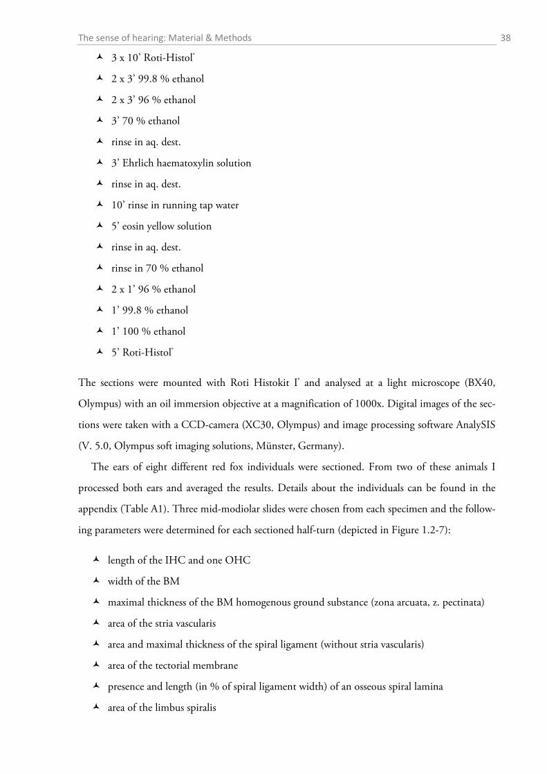
The sense of hearing: Material & Methods 38
3 x 10’ Roti-Histol®
2 x 3’ 99.8 % ethanol
2 x 3’ 96 % ethanol
3’ 70 % ethanol
rinse in aq. dest.
3’ Ehrlich haematoxylin solution
rinse in aq. dest.
10’ rinse in running tap water
5’ eosin yellow solution
rinse in aq. dest.
rinse in 70 % ethanol
2 x 1’ 96 % ethanol
1’ 99.8 % ethanol
1’ 100 % ethanol
5’ Roti-Histol®
The sections were mounted with Roti Histokit I® and analysed at a light microscope (BX40,
Olympus) with an oil immersion objective at a magnification of 1000x. Digital images of the sec-
tions were taken with a CCD-camera (XC30, Olympus) and image processing software AnalySIS
(V. 5.0, Olympus soft imaging solutions, Münster, Germany).
The ears of eight different red fox individuals were sectioned. From two of these animals I
processed both ears and averaged the results. Details about the individuals can be found in the
appendix (Table A1). Three mid-modiolar slides were chosen from each specimen and the follow-
ing parameters were determined for each sectioned half-turn (depicted in Figure 1.2-7):
length of the IHC and one OHC
width of the BM
maximal thickness of the BM homogenous ground substance (zona arcuata, z. pectinata)
area of the stria vascularis
area and maximal thickness of the spiral ligament (without stria vascularis)
area of the tectorial membrane
presence and length (in % of spiral ligament width) of an osseous spiral lamina
area of the limbus spiralis
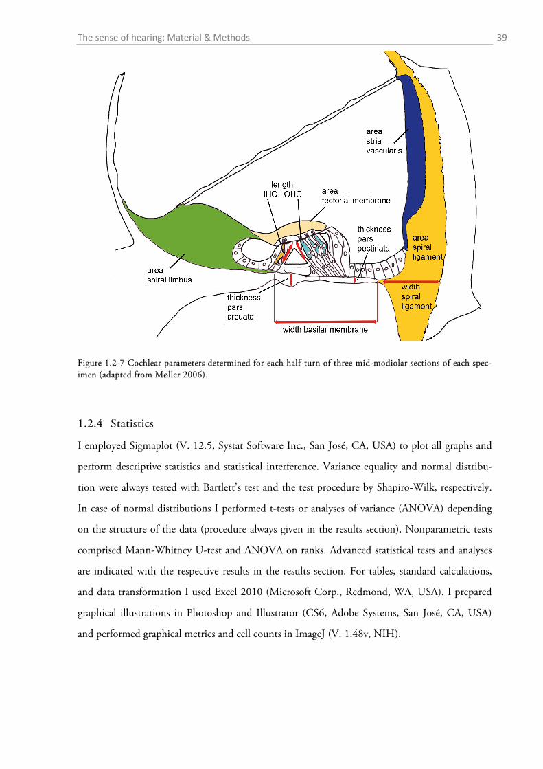
The sense of hearing: Material & Methods 39
Figure 1.2-7 Cochlear parameters determined for each half-turn of three mid-modiolar sections of each spec-imen (adapted from Møller 2006).
1.2.4 Statistics
I employed Sigmaplot (V. 12.5, Systat Software Inc., San José, CA, USA) to plot all graphs and
perform descriptive statistics and statistical interference. Variance equality and normal distribu-
tion were always tested with Bartlett’s test and the test procedure by Shapiro-Wilk, respectively.
In case of normal distributions I performed t-tests or analyses of variance (ANOVA) depending
on the structure of the data (procedure always given in the results section). Nonparametric tests
comprised Mann-Whitney U-test and ANOVA on ranks. Advanced statistical tests and analyses
are indicated with the respective results in the results section. For tables, standard calculations,
and data transformation I used Excel 2010 (Microsoft Corp., Redmond, WA, USA). I prepared
graphical illustrations in Photoshop and Illustrator (CS6, Adobe Systems, San José, CA, USA)
and performed graphical metrics and cell counts in ImageJ (V. 1.48v, NIH).
The sense of hearing: Results 40
1.3 Results
1.3.1 Behavioural audiometry
BEHAVIOURAL AUDIOGRAM
With two daily training sessions the foxes readily learned the behavioural procedure within 2-4
weeks. After the training period, up to two thresholds could be obtained per day, leading to a to-
tal experimental period of 8-10 weeks per animal. Complete audiograms could be obtained for
two animals, one fox (male 2) escaped from the enclosure during the experimental period. Hence,
from male 2 we could only obtain threshold values in the region of highest sensitivity (2 kHz,
4 kHz, 6.3 kHz, 8 kHz) and around the upper limit of hearing (46 kHz, 54 kHz) that were also
included in the calculation of the mean red fox audiogram.
The mean false alarm rates of all test sessions used for threshold determination were 13 %,
14 %, and 12 % for each of the three foxes, respectively (cf. Table 2). Furthermore, due to the
stability criterion and the correction for false alarms, 93 % of these test sessions had false alarm
rates lower than 20 %.
The thresholds of the individual foxes showed high conformity at most frequencies. The
mean red fox audiogram shows the typical mammalian V-shape (Figure 1.3-1; Table 2;
Fay 1988). At 60 dB SPL, a low frequency limit at 51 Hz was observed, while a gradual decrease
in thresholds led to the point of highest sensitivity with a mean of -15 dB SPL at 4 kHz for all
three animals. Two of the three animals showed comparable high sensitivity at 2 kHz and
6.3 kHz. The high mean sensitivity at those three frequencies was -10 dB SPL. Above 6.3 kHz,
however, sensitivity markedly dropped to 2 dB SPL at 8 kHz followed by a gradual increase of
the thresholds with retained sensitivity up to 40 kHz. Above this frequency, a steep increase of
thresholds led to a quick approach of the 60 dB SPL high frequency limit at 48 kHz. At
60 dB SPL the red fox audiogram spans 9.84 octaves.
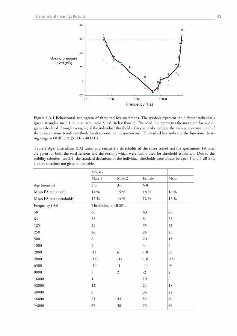
The sense of hearing: Results 41
Figure 1.3-1 Behavioural audiogram of three red fox specimens. The symbols represent the different individuals (green triangles: male 1; blue squares: male 2; red circles: female). The solid line represents the mean red fox audio-gram calculated through averaging of the individual thresholds. Grey asterisks indicate the average spectrum level of the ambient noise (confer methods for details on the measurements). The dashed line indicates the functional hear-ing range at 60 dB SPL (51 Hz - 48 kHz). Table 2 Age, false alarm (FA) rates, and sensitivity thresholds of the three tested red fox specimens. FA rates are given for both the total sessions and the sessions which were finally used for threshold estimation. Due to the stability criterion (see 2.4) the standard deviations of the individual thresholds were always between 1 and 5 dB SPL and are therefore not given in the table.
Subject
Male 1 Male 2 Female Mean
Age (months) 3-5 3-5 6-8
Mean FA rate (total) 14 % 15 % 18 % 16 %
Mean FA rate (thresholds) 13 % 14 % 12 % 13 %
Frequency (Hz) Thresholds in dB SPL
50 66 60 63
63 55 51 53
125 29 35 32
250 26 24 25
500 6 20 13
1000 5 4 5
2000 -11 6 -10 -5
4000 -14 -14 -16 -15
6300 -14 -1 -11 -9
8000 5 2 -2 2
16000 1 10 6
32000 12 24 18
40000 9 34 22
46000 21 44 54 40
54000 67 58 73 66
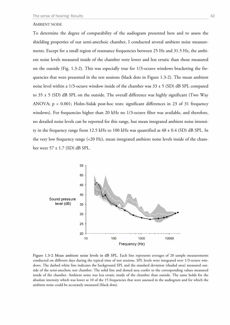
The sense of hearing: Results 42
AMBIENT NOISE
To determine the degree of comparability of the audiogram presented here and to assess the
shielding properties of our semi-anechoic chamber, I conducted several ambient noise measure-
ments. Except for a small region of resonance frequencies between 25 Hz and 31.5 Hz, the ambi-
ent noise levels measured inside of the chamber were lower and less erratic than those measured
on the outside (Fig. 1.3-2). This was especially true for 1/3-octave windows bracketing the fre-
quencies that were presented in the test sessions (black dots in Figure 1.3-2). The mean ambient
noise level within a 1/3-octave window inside of the chamber was 33 ± 5 (SD) dB SPL compared
to 35 ± 5 (SD) dB SPL on the outside. The overall difference was highly significant (Two Way
ANOVA; p < 0.001; Holm-Sidak post-hoc tests: significant differences in 23 of 31 frequency
windows). For frequencies higher than 20 kHz no 1/3-octave filter was available, and therefore,
no detailed noise levels can be reported for this range, but mean integrated ambient noise intensi-
ty in the frequency range from 12.5 kHz to 100 kHz was quantified as 48 ± 0.4 (SD) dB SPL. In
the very low frequency range (<20 Hz), mean integrated ambient noise levels inside of the cham-
ber were 57 ± 1.7 (SD) dB SPL.
Figure 1.3-2 Mean ambient noise levels in dB SPL. Each line represents averages of 20 sample measurements conducted on different days during the typical time of test sessions. SPL levels were integrated over 1/3-octave win-dows. The dashed white line indicates the background SPL and the standard deviation (shaded area) measured out-side of the semi-anechoic test chamber. The solid line and dotted area confer to the corresponding values measured inside of the chamber. Ambient noise was less erratic inside of the chamber than outside. The same holds for the absolute intensity which was lower at 10 of the 15 frequencies that were assessed in the audiogram and for which the ambient noise could be accurately measured (black dots).
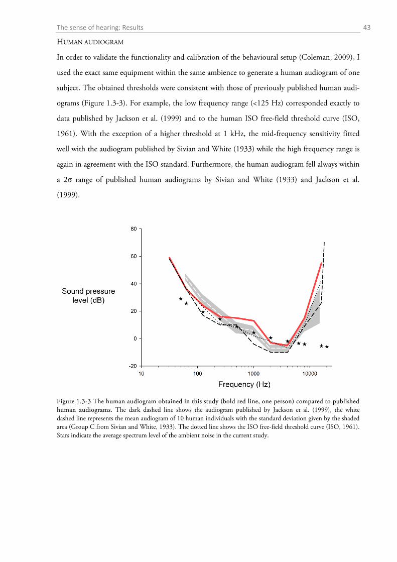
The sense of hearing: Results 43
HUMAN AUDIOGRAM
In order to validate the functionality and calibration of the behavioural setup (Coleman, 2009), I
used the exact same equipment within the same ambience to generate a human audiogram of one
subject. The obtained thresholds were consistent with those of previously published human audi-
ograms (Figure 1.3-3). For example, the low frequency range (<125 Hz) corresponded exactly to
data published by Jackson et al. (1999) and to the human ISO free-field threshold curve (ISO,
1961). With the exception of a higher threshold at 1 kHz, the mid-frequency sensitivity fitted
well with the audiogram published by Sivian and White (1933) while the high frequency range is
again in agreement with the ISO standard. Furthermore, the human audiogram fell always within
a 2σ range of published human audiograms by Sivian and White (1933) and Jackson et al.
(1999).
Figure 1.3-3 The human audiogram obtained in this study (bold red line, one person) compared to published human audiograms. The dark dashed line shows the audiogram published by Jackson et al. (1999), the white dashed line represents the mean audiogram of 10 human individuals with the standard deviation given by the shaded area (Group C from Sivian and White, 1933). The dotted line shows the ISO free-field threshold curve (ISO, 1961). Stars indicate the average spectrum level of the ambient noise in the current study.
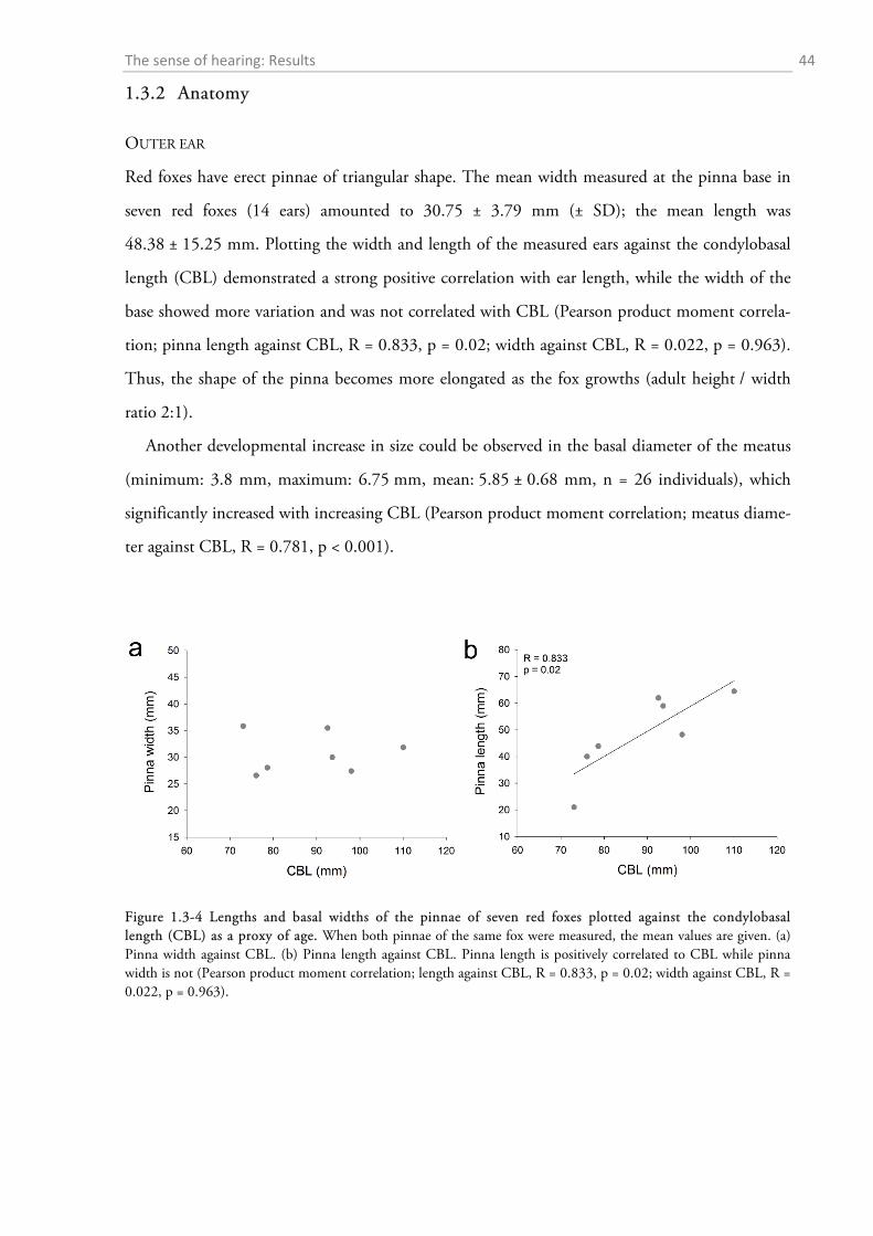
The sense of hearing: Results 44
1.3.2 Anatomy
OUTER EAR
Red foxes have erect pinnae of triangular shape. The mean width measured at the pinna base in
seven red foxes (14 ears) amounted to 30.75 ± 3.79 mm (± SD); the mean length was
48.38 ± 15.25 mm. Plotting the width and length of the measured ears against the condylobasal
length (CBL) demonstrated a strong positive correlation with ear length, while the width of the
base showed more variation and was not correlated with CBL (Pearson product moment correla-
tion; pinna length against CBL, R = 0.833, p = 0.02; width against CBL, R = 0.022, p = 0.963).
Thus, the shape of the pinna becomes more elongated as the fox growths (adult height / width
ratio 2:1).
Another developmental increase in size could be observed in the basal diameter of the meatus
(minimum: 3.8 mm, maximum: 6.75 mm, mean: 5.85 ± 0.68 mm, n = 26 individuals), which
significantly increased with increasing CBL (Pearson product moment correlation; meatus diame-
ter against CBL, R = 0.781, p < 0.001).
Figure 1.3-4 Lengths and basal widths of the pinnae of seven red foxes plotted against the condylobasal length (CBL) as a proxy of age. When both pinnae of the same fox were measured, the mean values are given. (a) Pinna width against CBL. (b) Pinna length against CBL. Pinna length is positively correlated to CBL while pinna width is not (Pearson product moment correlation; length against CBL, R = 0.833, p = 0.02; width against CBL, R = 0.022, p = 0.963).
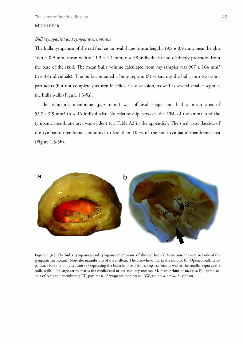
The sense of hearing: Results 45
MIDDLE EAR
Bulla tympanica and tympanic membrane
The bulla tympanica of the red fox has an oval shape (mean length: 19.8 ± 0.9 mm, mean height:
16.4 ± 0.9 mm, mean width: 11.3 ± 1.1 mm; n = 38 individuals) and distinctly protrudes from
the base of the skull. The mean bulla volume calculated from my samples was 967 ± 164 mm³
(n = 38 individuals). The bulla contained a bony septum (S) separating the bulla into two com-
partments (but not completely as seen in felids, see discussion) as well as several smaller septa at
the bulla walls (Figure 1.3-5a).
The tympanic membrane (pars tensa) was of oval shape and had a mean area of
55.7 ± 7.9 mm² (n = 16 individuals). No relationship between the CBL of the animal and the
tympanic membrane area was evident (cf. Table A2 in the appendix). The small pars flaccida of
the tympanic membrane amounted to less than 10 % of the total tympanic membrane area
(Figure 1.3-5b).
Figure 1.3-5 The bulla tympanica and tympanic membrane of the red fox. (a) View onto the external side of the tympanic membrane. Note the manubrium of the malleus. The arrowhead marks the umbro. (b) Opened bulla tym-panica. Note the bony septum (S) separating the bulla into two half-compartments as well as the smaller septa at the bulla walls. The large arrow marks the medial end of the auditory meatus. M, manubrium of malleus; PF, pars flac-cida of tympanic membrane; PT, pars tensa of tympanic membrane; RW, round window; S, septum.
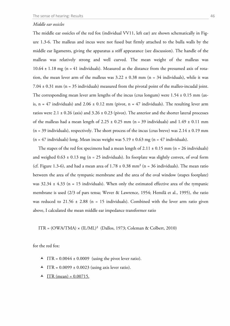
The sense of hearing: Results 46
Middle ear ossicles
The middle ear ossicles of the red fox (individual VV11, left ear) are shown schematically in Fig-
ure 1.3-6. The malleus and incus were not fused but firmly attached to the bulla walls by the
middle ear ligaments, giving the apparatus a stiff appearance (see discussion). The handle of the
malleus was relatively strong and well curved. The mean weight of the malleus was
10.64 ± 1.18 mg (n = 41 individuals). Measured as the distance from the presumed axis of rota-
tion, the mean lever arm of the malleus was 3.22 ± 0.38 mm (n = 34 individuals), while it was
7.04 ± 0.31 mm (n = 35 individuals) measured from the pivotal point of the malleo-incudal joint.
The corresponding mean lever arm lengths of the incus (crus longum) were 1.54 ± 0.15 mm (ax-
is, n = 47 individuals) and 2.06 ± 0.12 mm (pivot, n = 47 individuals). The resulting lever arm
ratios were 2.1 ± 0.26 (axis) and 3.26 ± 0.23 (pivot). The anterior and the shorter lateral processes
of the malleus had a mean length of 2.25 ± 0.25 mm (n = 39 individuals) and 1.49 ± 0.11 mm
(n = 39 individuals), respectively. The short process of the incus (crus breve) was 2.14 ± 0.19 mm
(n = 47 individuals) long. Mean incus weight was 5.19 ± 0.63 mg (n = 47 individuals).
The stapes of the red fox specimens had a mean length of 2.11 ± 0.15 mm (n = 26 individuals)
and weighed 0.63 ± 0.13 mg (n = 25 individuals). Its footplate was slightly convex, of oval form
(cf. Figure 1.3-6), and had a mean area of 1.78 ± 0.38 mm² (n = 36 individuals). The mean ratio
between the area of the tympanic membrane and the area of the oval window (stapes footplate)
was 32.34 ± 4.33 (n = 15 individuals). When only the estimated effective area of the tympanic
membrane is used (2/3 of pars tensa; Wever & Lawrence, 1954; Hemilä et al., 1995), the ratio
was reduced to 21.56 ± 2.88 (n = 15 individuals). Combined with the lever arm ratio given
above, I calculated the mean middle ear impedance transformer ratio
ITR = (OWA/TMA) × (IL/ML)² (Dallos, 1973; Coleman & Colbert, 2010)
for the red fox:
ITR = 0.0044 ± 0.0009 (using the pivot lever ratio).
ITR = 0.0099 ± 0.0023 (using axis lever ratio).
ITR (mean) = 0.00715.
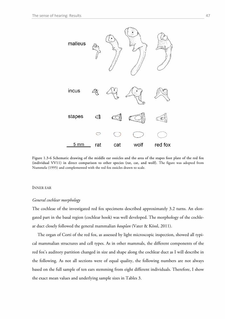
The sense of hearing: Results 47
Figure 1.3-6 Schematic drawing of the middle ear ossicles and the area of the stapes foot plate of the red fox (individual VV11) in direct comparison to other species (rat, cat, and wolf). The figure was adopted from Nummela (1995) and complemented with the red fox ossicles drawn to scale.
INNER EAR
General cochlear morphology
The cochleae of the investigated red fox specimens described approximately 3.2 turns. An elon-
gated part in the basal region (cochlear hook) was well developed. The morphology of the cochle-
ar duct closely followed the general mammalian bauplan (Vater & Kössl, 2011).
The organ of Corti of the red fox, as assessed by light microscopic inspection, showed all typi-
cal mammalian structures and cell types. As in other mammals, the different components of the
red fox’s auditory partition changed in size and shape along the cochlear duct as I will describe in
the following. As not all sections were of equal quality, the following numbers are not always
based on the full sample of ten ears stemming from eight different individuals. Therefore, I show
the exact mean values and underlying sample sizes in Tables 3.
The sense of hearing: Results 48
The base of the cochlea was characterised by an osseous spiral lamina considerably protruding
into the cochlear duct, supporting the spiral ligament along almost 100 % of its width, all the
way to the outer edge of the BM. This support was retracted further up the cochlear duct and was
completely absent somewhere between the fourth and fifth (~ 16 mm from the base) half-turn
(HT). From here on up to the apical end, the basilar membrane was supported on its external
edge only by the spiral ligament. In the upper HTs, however, the spiral ligament reached down to
the floor of the scala tympani (Figure 1.3-7, inset d), which might substitute for the support of
the osseous spiral lamina.
The cross sectional areas of the tectorial membrane and the spiral limbus changed with re-
versed gradients. The tectorial membrane area increased considerably from the base (835 µm²;
confer Table 3 for standard deviations) towards the sixth HT (7,870 µm²) and slightly decreased
afterwards (6,457 µm²). The spiral limbus showed relatively constant cross sectional areas up to
the second HT and from thereon steadily decreased in size (~ 22,000-6,500 µm²).
The spiral ligament decreased in size towards the apex of the cochlea, as reflected by a decrease
of both width and area. The width declined from a basal value of 424 µm to roughly one fifth of
this value at the apex (82 µm). The area decreased accordingly, from more than 160,000 µm² at
the base, down to 20,000 µm² in apical regions. Accordingly, also the absolute cross sectional area
of the stria vascularis decreased from basal values around 12,000-13,000 µm² down to 2,500-
3,000 µm². The proportion of the stria vascularis relative to the spiral ligament, however, dou-
bled from basal ~ 8 % to 15-20 % in apical regions.
The BM reached a maximal thickness (mean: 17.7 µm; both partes pectinata and arcuata) in
the region of the first HT. Further basalward the thickness slightly decreased in the order of
1-2 µm. From the first HT towards the apex, the thickness of the BM decreased constantly until
it reached minimal thickness of 5-6 µm in apical regions. The slope of the decline was slightly
steeper in pars pectinata than pars arcuata. The decrease in BM thickness towards the apical end
was accompanied by an increase in BM width, which was smallest in the hook region (~ 80 µm)
and reached widths of more than 380 µm near the apex. The stiffness ratio f (thickness BM /
width BM; von Békésy, 1960) decreased constantly from a basal value of ~ 0.19 to an apical value
of 0.015 (fbasal : fapical = 13:1).
Even though the figures are based on a relatively small sample (cf. Table 3), it was indicated
that the length of the IHCs underwent no change along the cochlear duct (stable length around
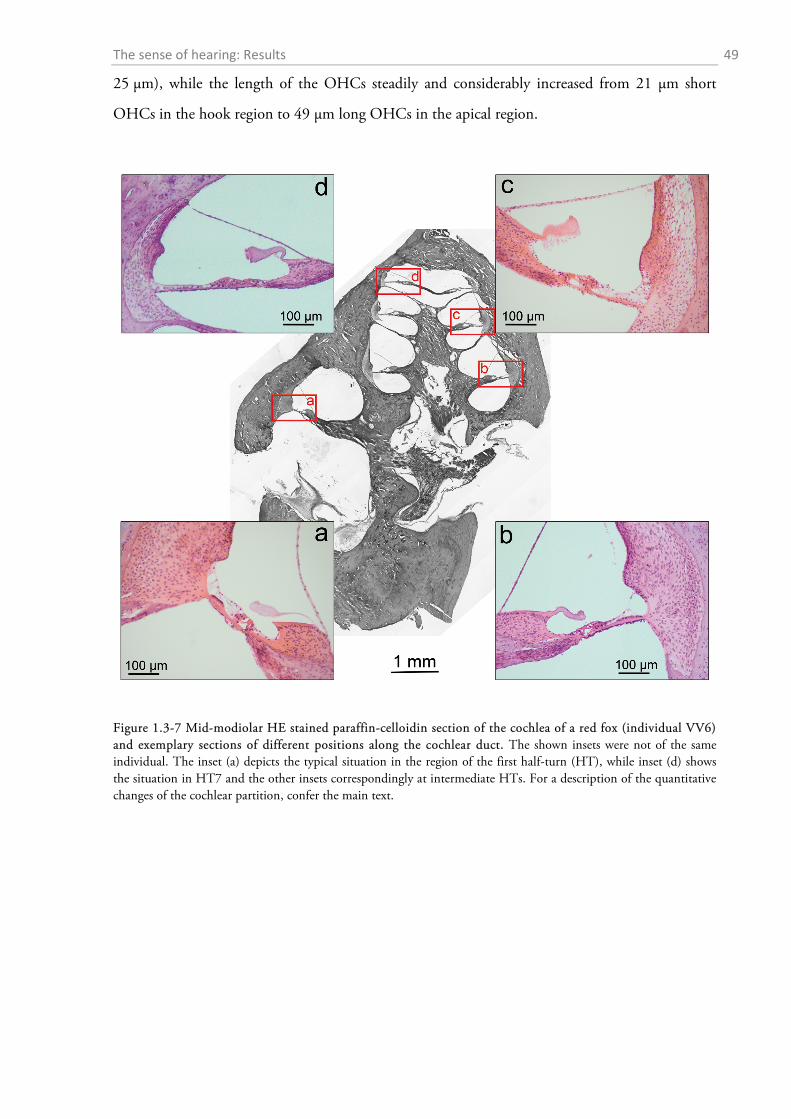
The sense of hearing: Results 49
25 µm), while the length of the OHCs steadily and considerably increased from 21 µm short
OHCs in the hook region to 49 µm long OHCs in the apical region.
Figure 1.3-7 Mid-modiolar HE stained paraffin-celloidin section of the cochlea of a red fox (individual VV6) and exemplary sections of different positions along the cochlear duct. The shown insets were not of the same individual. The inset (a) depicts the typical situation in the region of the first half-turn (HT), while inset (d) shows the situation in HT7 and the other insets correspondingly at intermediate HTs. For a description of the quantitative changes of the cochlear partition, confer the main text.
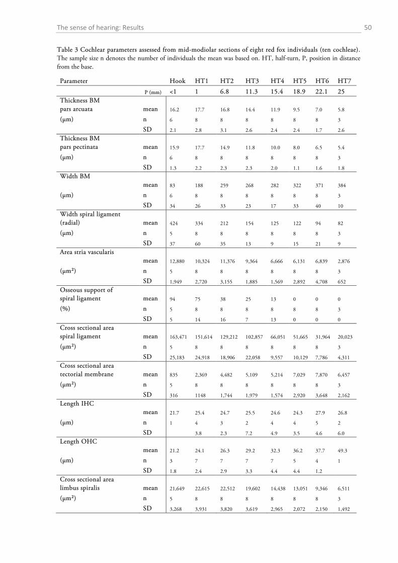
The sense of hearing: Results 50
Table 3 Cochlear parameters assessed from mid-modiolar sections of eight red fox individuals (ten cochleae). The sample size n denotes the number of individuals the mean was based on. HT, half-turn, P, position in distance from the base.
Parameter Hook HT1 HT2 HT3 HT4 HT5 HT6 HT7
P (mm) <1 1 6.8 11.3 15.4 18.9 22.1 25 Thickness BM pars arcuata mean 16.2 17.7 16.8 14.4 11.9 9.5 7.0 5.8
(µm) n 6 8 8 8 8 8 8 3
SD 2.1 2.8 3.1 2.6 2.4 2.4 1.7 2.6 Thickness BM pars pectinata mean 15.9 17.7 14.9 11.8 10.0 8.0 6.5 5.4
(µm) n 6 8 8 8 8 8 8 3
SD 1.3 2.2 2.3 2.3 2.0 1.1 1.6 1.8 Width BM mean 83 188 259 268 282 322 371 384
(µm) n 6 8 8 8 8 8 8 3
SD 34 26 33 23 17 33 40 10 Width spiral ligament (radial) mean 424 334 212 154 125 122 94 82
(µm) n 5 8 8 8 8 8 8 3
SD 37 60 35 13 9 15 21 9 Area stria vascularis mean 12,880 10,324 11,376 9,364 6,666 6,131 6,839 2,876
(µm²) n 5 8 8 8 8 8 8 3
SD 1,949 2,720 3,155 1,885 1,569 2,892 4,708 652 Osseous support of spiral ligament mean 94 75 38 25 13 0 0 0
(%) n 5 8 8 8 8 8 8 3
SD 5 14 16 7 13 0 0 0 Cross sectional area spiral ligament mean 163,471 151,614 129,212 102,857 66,051 51,665 31,964 20,023
(µm²) n 5 8 8 8 8 8 8 3
SD 25,183 24,918 18,906 22,058 9,557 10,129 7,786 4,311 Cross sectional area tectorial membrane mean 835 2,369 4,482 5,109 5,214 7,029 7,870 6,457
(µm²) n 5 8 8 8 8 8 8 3
SD 316 1148 1,744 1,979 1,574 2,920 3,648 2,162 Length IHC mean 21.7 25.4 24.7 25.5 24.6 24.3 27.9 26.8
(µm) n 1 4 3 2 4 4 5 2
SD 3.8 2.3 7.2 4.9 3.5 4.6 6.0 Length OHC mean 21.2 24.1 26.3 29.2 32.3 36.2 37.7 49.3
(µm) n 3 7 7 7 7 5 4 1
SD 1.8 2.4 2.9 3.3 4.4 4.4 1.2 Cross sectional area limbus spiralis mean 21,649 22,615 22,512 19,602 14,438 13,051 9,346 6,511
(µm²) n 5 8 8 8 8 8 8 3
SD 3,268 3,931 3,820 3,619 2,965 2,072 2,150 1,492
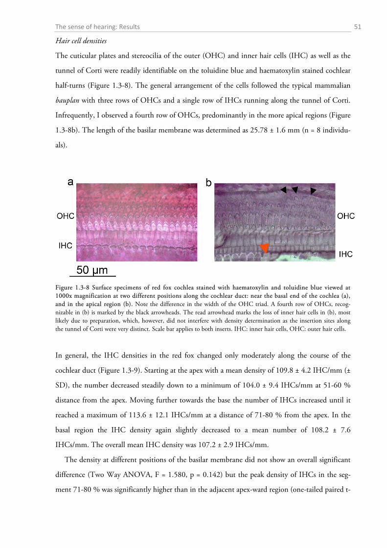
The sense of hearing: Results 51
Hair cell densities
The cuticular plates and stereocilia of the outer (OHC) and inner hair cells (IHC) as well as the
tunnel of Corti were readily identifiable on the toluidine blue and haematoxylin stained cochlear
half-turns (Figure 1.3-8). The general arrangement of the cells followed the typical mammalian
bauplan with three rows of OHCs and a single row of IHCs running along the tunnel of Corti.
Infrequently, I observed a fourth row of OHCs, predominantly in the more apical regions (Figure
1.3-8b). The length of the basilar membrane was determined as 25.78 ± 1.6 mm (n = 8 individu-
als).
Figure 1.3-8 Surface specimens of red fox cochlea stained with haematoxylin and toluidine blue viewed at 1000x magnification at two different positions along the cochlear duct: near the basal end of the cochlea (a), and in the apical region (b). Note the difference in the width of the OHC triad. A fourth row of OHCs, recog-nizable in (b) is marked by the black arrowheads. The read arrowhead marks the loss of inner hair cells in (b), most likely due to preparation, which, however, did not interfere with density determination as the insertion sites along the tunnel of Corti were very distinct. Scale bar applies to both inserts. IHC: inner hair cells, OHC: outer hair cells.
In general, the IHC densities in the red fox changed only moderately along the course of the
cochlear duct (Figure 1.3-9). Starting at the apex with a mean density of 109.8 ± 4.2 IHC/mm (±
SD), the number decreased steadily down to a minimum of 104.0 ± 9.4 IHCs/mm at 51-60 %
distance from the apex. Moving further towards the base the number of IHCs increased until it
reached a maximum of 113.6 ± 12.1 IHCs/mm at a distance of 71-80 % from the apex. In the
basal region the IHC density again slightly decreased to a mean number of 108.2 ± 7.6
IHCs/mm. The overall mean IHC density was 107.2 ± 2.9 IHCs/mm.
The density at different positions of the basilar membrane did not show an overall significant
difference (Two Way ANOVA, F = 1.580, p = 0.142) but the peak density of IHCs in the seg-
ment 71-80 % was significantly higher than in the adjacent apex-ward region (one-tailed paired t-
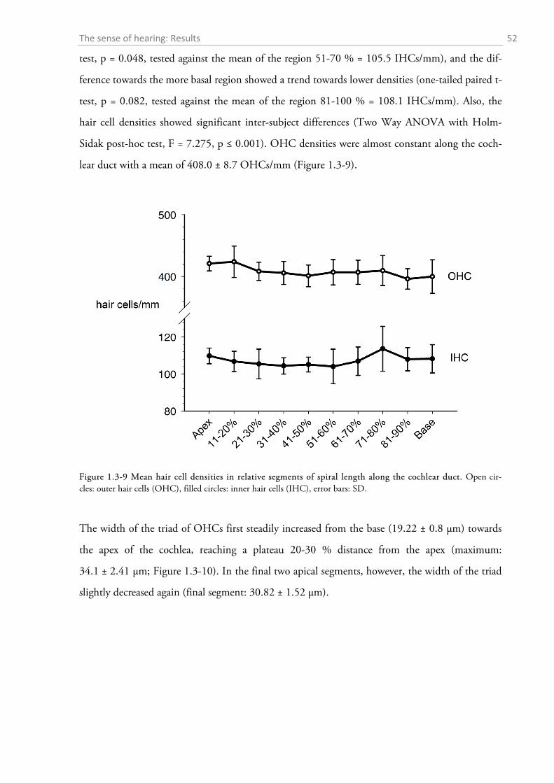
The sense of hearing: Results 52
test, p = 0.048, tested against the mean of the region 51-70 % = 105.5 IHCs/mm), and the dif-
ference towards the more basal region showed a trend towards lower densities (one-tailed paired t-
test, p = 0.082, tested against the mean of the region 81-100 % = 108.1 IHCs/mm). Also, the
hair cell densities showed significant inter-subject differences (Two Way ANOVA with Holm-
Sidak post-hoc test, F = 7.275, p ≤ 0.001). OHC densities were almost constant along the coch-
lear duct with a mean of 408.0 ± 8.7 OHCs/mm (Figure 1.3-9).
Figure 1.3-9 Mean hair cell densities in relative segments of spiral length along the cochlear duct. Open cir-cles: outer hair cells (OHC), filled circles: inner hair cells (IHC), error bars: SD.
The width of the triad of OHCs first steadily increased from the base (19.22 ± 0.8 µm) towards
the apex of the cochlea, reaching a plateau 20-30 % distance from the apex (maximum:
34.1 ± 2.41 µm; Figure 1.3-10). In the final two apical segments, however, the width of the triad
slightly decreased again (final segment: 30.82 ± 1.52 µm).
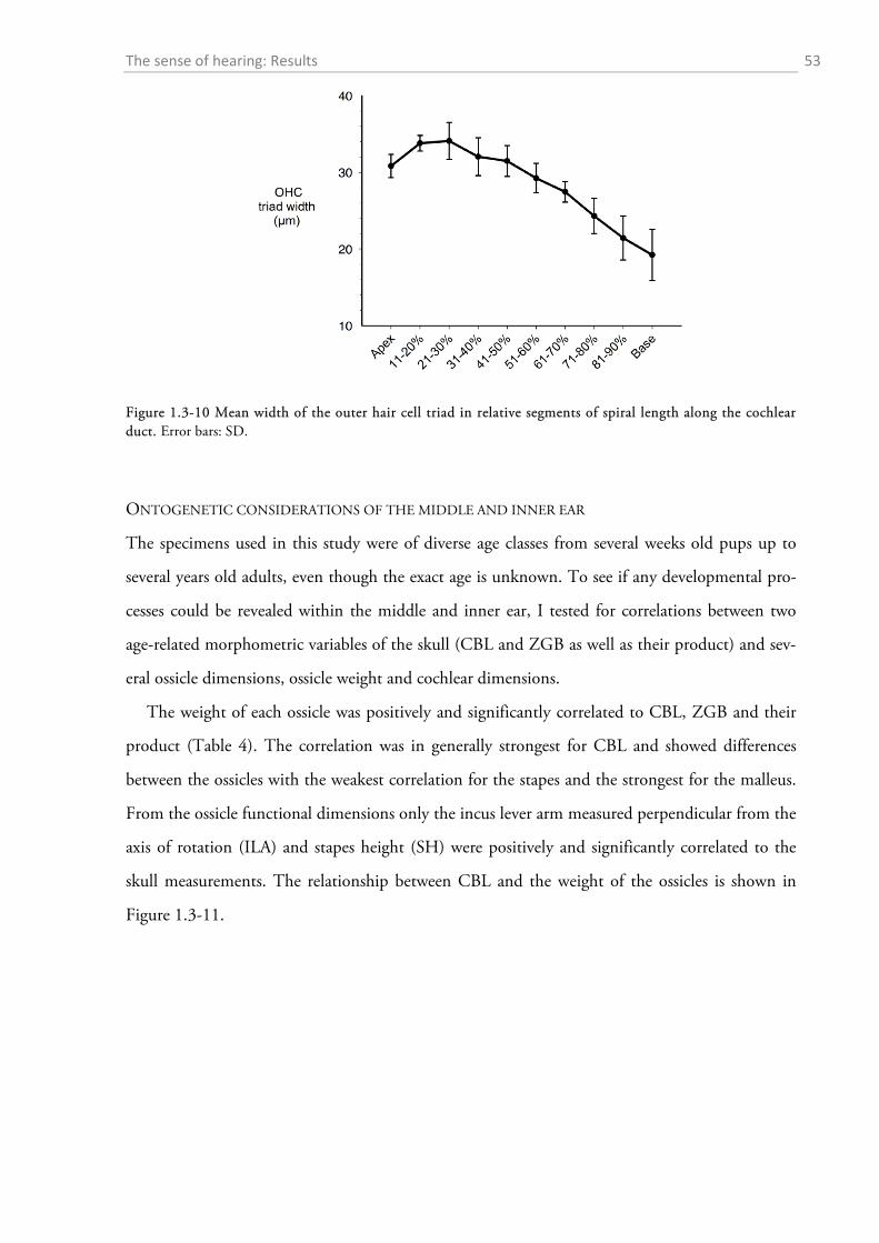
The sense of hearing: Results 53
Figure 1.3-10 Mean width of the outer hair cell triad in relative segments of spiral length along the cochlear duct. Error bars: SD.
ONTOGENETIC CONSIDERATIONS OF THE MIDDLE AND INNER EAR
The specimens used in this study were of diverse age classes from several weeks old pups up to
several years old adults, even though the exact age is unknown. To see if any developmental pro-
cesses could be revealed within the middle and inner ear, I tested for correlations between two
age-related morphometric variables of the skull (CBL and ZGB as well as their product) and sev-
eral ossicle dimensions, ossicle weight and cochlear dimensions.
The weight of each ossicle was positively and significantly correlated to CBL, ZGB and their
product (Table 4). The correlation was in generally strongest for CBL and showed differences
between the ossicles with the weakest correlation for the stapes and the strongest for the malleus.
From the ossicle functional dimensions only the incus lever arm measured perpendicular from the
axis of rotation (ILA) and stapes height (SH) were positively and significantly correlated to the
skull measurements. The relationship between CBL and the weight of the ossicles is shown in
Figure 1.3-11.
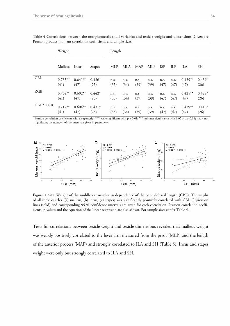
The sense of hearing: Results 54
Table 4 Correlations between the morphometric skull variables and ossicle weight and dimensions. Given are Pearson product-moment correlation coefficients and sample sizes.
Weight
Length
Malleus Incus Stapes MLP MLA MAP MLP ISP ILP ILA SH
CBL 0.735** (41)
0.641** (47)
0.426* (25)
n.s. (35)
n.s. (34)
n.s. (39)
n.s. (39)
n.s. (47)
n.s. (47)
0.439** (47)
0.439* (26)
ZGB 0.708** (41)
0.602** (47)
0.442* (25)
n.s. (35)
n.s. (34)
n.s (39)
n.s. (39)
n.s. (47)
n.s. (47)
0.425** (47)
0.429* (26)
CBL * ZGB 0.712** (41)
0.604** (47)
0.431* (25)
n.s. (35)
n.s. (34)
n.s (39)
n.s. (39)
n.s. (47)
n.s. (47)
0.429** (47)
0.418* (26)
Pearson correlation coefficients with a superscript "**" were significant with p < 0.01; "*" indicates significance with 0.05 > p > 0.01; n.s. = not significant; the numbers of specimens are given in parentheses
Figure 1.3-11 Weight of the middle ear ossicles in dependence of the condylobasal length (CBL). The weight of all three ossicles ((a) malleus, (b) incus, (c) stapes) was significantly positively correlated with CBL. Regression lines (solid) and corresponding 95 %-confidence intervals are given for each correlation. Pearson correlation coeffi-cients, p-values and the equation of the linear regression are also shown. For sample sizes confer Table 4.
Tests for correlations between ossicle weight and ossicle dimensions revealed that malleus weight
was weakly positively correlated to the lever arm measured from the pivot (MLP) and the length
of the anterior process (MAP) and strongly correlated to ILA and SH (Table 5). Incus and stapes
weight were only but strongly correlated to ILA and SH.
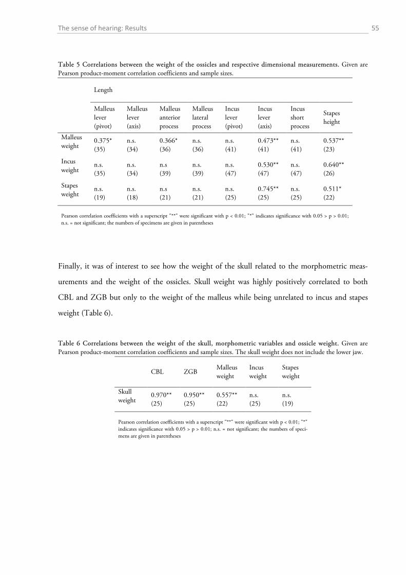
The sense of hearing: Results 55
Table 5 Correlations between the weight of the ossicles and respective dimensional measurements. Given are Pearson product-moment correlation coefficients and sample sizes.
Length
Malleus lever (pivot)
Malleus lever (axis)
Malleus anterior process
Malleus lateral process
Incus lever (pivot)
Incus lever (axis)
Incus short process
Stapes height
Malleus weight
0.375* (35)
n.s. (34)
0.366* (36)
n.s. (36)
n.s. (41)
0.473** (41)
n.s. (41)
0.537** (23)
Incus weight
n.s. (35)
n.s. (34)
n.s (39)
n.s. (39)
n.s. (47)
0.530** (47)
n.s. (47)
0.640** (26)
Stapes weight
n.s. (19)
n.s. (18)
n.s (21)
n.s. (21)
n.s. (25)
0.745** (25)
n.s. (25)
0.511* (22)
Pearson correlation coefficients with a superscript "**" were significant with p < 0.01; "*" indicates significance with 0.05 > p > 0.01; n.s. = not significant; the numbers of specimens are given in parentheses
Finally, it was of interest to see how the weight of the skull related to the morphometric meas-
urements and the weight of the ossicles. Skull weight was highly positively correlated to both
CBL and ZGB but only to the weight of the malleus while being unrelated to incus and stapes
weight (Table 6).
Table 6 Correlations between the weight of the skull, morphometric variables and ossicle weight. Given are Pearson product-moment correlation coefficients and sample sizes. The skull weight does not include the lower jaw.
CBL ZGB Malleus weight
Incus weight
Stapes weight
Skull weight
0.970** (25)
0.950** (25)
0.557** (22)
n.s. (25)
n.s. (19)
Pearson correlation coefficients with a superscript "**" were significant with p < 0.01; "*" indicates significance with 0.05 > p > 0.01; n.s. = not significant; the numbers of speci-mens are given in parentheses
The sense of hearing: Discussion 56
1.4 Discussion
1.4.1 Behavioural audiometry
FUNCTIONALITY OF THE SETUP AND EFFICIENCY OF THE PSYCHOPHYSICAL PROCEDURE
Several classical and operant conditioning methods are suitable for the assessment of valid animal
audiograms (Fay, 1988; Klump et al., 1995). These include both negative conditioning methods
such as conditioned avoidance, and positive methods based on reward paradigms. In addition, the
method of conditioned suppression represents a powerful combination of both positive and nega-
tive reinforcement (Smith, 1970). Each method has its advantages and disadvantages with regards
to training time, subject control and the efficiency of data collection. As long as certain standard
criteria are met, however, the resulting audiogram data are mostly independent of the condition-
ing method and provides comparable results (Fujita & Elliott, 1965; Green, 1975; Fay, 1992;
Coleman, 2009).
Here, I chose a reward-based (positive) conditioning method because it is more efficient and
provides more stable results compared to avoidance procedures, while also avoiding long lasting
adverse behavioural consequences (e.g. increased aggressiveness; Stebbins et al., 1984). The latter
was of special importance as the subjects were neither laboratory animals nor completely wild and
were required to remain affable after completion of the auditory experiments.
Obtaining animal audiograms is a tedious task, consuming considerable time and energy to es-
tablish and to stabilize desired behaviours. On the other hand, it is rewarding, as auditory thresh-
olds between healthy individuals of the same species do not differ considerably, so that testing of
two to three individuals is sufficient to make generalizations about the species’ auditory sensitivity
especially in large and non-laboratory animals (Heffner & Heffner, 1988b, 2010).
Recently, Benovitski et al. (2014) developed a mobile apparatus, quite similar to the one I de-
signed, allowing researchers to perform psychoacoustic tests in cats without the need to monitor
the experiment continuously and with the great advantage that the animals are free to decide how
often and when they would like to perform. The authors also employed a simple go/no-go task
with food as a reward. In simple frequency discrimination tasks their technique yielded fast and
stable data which were in line with previously published results. As their setup did not provide
acoustic shielding, the performing subjects, however, were prone to distractions from other sound
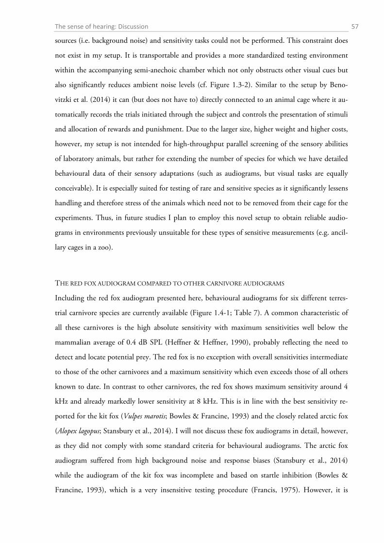
The sense of hearing: Discussion 57
sources (i.e. background noise) and sensitivity tasks could not be performed. This constraint does
not exist in my setup. It is transportable and provides a more standardized testing environment
within the accompanying semi-anechoic chamber which not only obstructs other visual cues but
also significantly reduces ambient noise levels (cf. Figure 1.3-2). Similar to the setup by Beno-
vitzki et al. (2014) it can (but does not have to) directly connected to an animal cage where it au-
tomatically records the trials initiated through the subject and controls the presentation of stimuli
and allocation of rewards and punishment. Due to the larger size, higher weight and higher costs,
however, my setup is not intended for high-throughput parallel screening of the sensory abilities
of laboratory animals, but rather for extending the number of species for which we have detailed
behavioural data of their sensory adaptations (such as audiograms, but visual tasks are equally
conceivable). It is especially suited for testing of rare and sensitive species as it significantly lessens
handling and therefore stress of the animals which need not to be removed from their cage for the
experiments. Thus, in future studies I plan to employ this novel setup to obtain reliable audio-
grams in environments previously unsuitable for these types of sensitive measurements (e.g. ancil-
lary cages in a zoo).
THE RED FOX AUDIOGRAM COMPARED TO OTHER CARNIVORE AUDIOGRAMS
Including the red fox audiogram presented here, behavioural audiograms for six different terres-
trial carnivore species are currently available (Figure 1.4-1; Table 7). A common characteristic of
all these carnivores is the high absolute sensitivity with maximum sensitivities well below the
mammalian average of 0.4 dB SPL (Heffner & Heffner, 1990), probably reflecting the need to
detect and locate potential prey. The red fox is no exception with overall sensitivities intermediate
to those of the other carnivores and a maximum sensitivity which even exceeds those of all others
known to date. In contrast to other carnivores, the red fox shows maximum sensitivity around 4
kHz and already markedly lower sensitivity at 8 kHz. This is in line with the best sensitivity re-
ported for the kit fox (Vulpes marotis; Bowles & Francine, 1993) and the closely related arctic fox
(Alopex lagopus; Stansbury et al., 2014). I will not discuss these fox audiograms in detail, however,
as they did not comply with some standard criteria for behavioural audiograms. The arctic fox
audiogram suffered from high background noise and response biases (Stansbury et al., 2014)
while the audiogram of the kit fox was incomplete and based on startle inhibition (Bowles &
Francine, 1993), which is a very insensitive testing procedure (Francis, 1975). However, it is
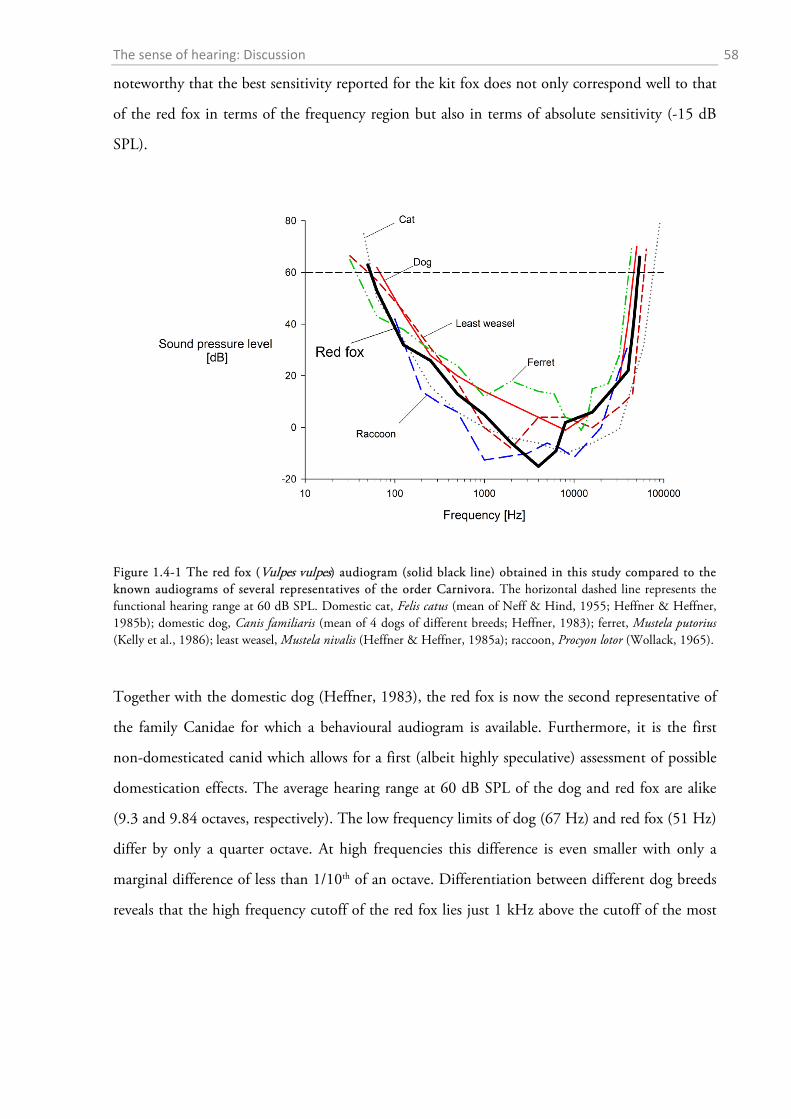
The sense of hearing: Discussion 58
noteworthy that the best sensitivity reported for the kit fox does not only correspond well to that
of the red fox in terms of the frequency region but also in terms of absolute sensitivity (-15 dB
SPL).
Figure 1.4-1 The red fox (Vulpes vulpes) audiogram (solid black line) obtained in this study compared to the known audiograms of several representatives of the order Carnivora. The horizontal dashed line represents the functional hearing range at 60 dB SPL. Domestic cat, Felis catus (mean of Neff & Hind, 1955; Heffner & Heffner, 1985b); domestic dog, Canis familiaris (mean of 4 dogs of different breeds; Heffner, 1983); ferret, Mustela putorius (Kelly et al., 1986); least weasel, Mustela nivalis (Heffner & Heffner, 1985a); raccoon, Procyon lotor (Wollack, 1965).
Together with the domestic dog (Heffner, 1983), the red fox is now the second representative of
the family Canidae for which a behavioural audiogram is available. Furthermore, it is the first
non-domesticated canid which allows for a first (albeit highly speculative) assessment of possible
domestication effects. The average hearing range at 60 dB SPL of the dog and red fox are alike
(9.3 and 9.84 octaves, respectively). The low frequency limits of dog (67 Hz) and red fox (51 Hz)
differ by only a quarter octave. At high frequencies this difference is even smaller with only a
marginal difference of less than 1/10th of an octave. Differentiation between different dog breeds
reveals that the high frequency cutoff of the red fox lies just 1 kHz above the cutoff of the most
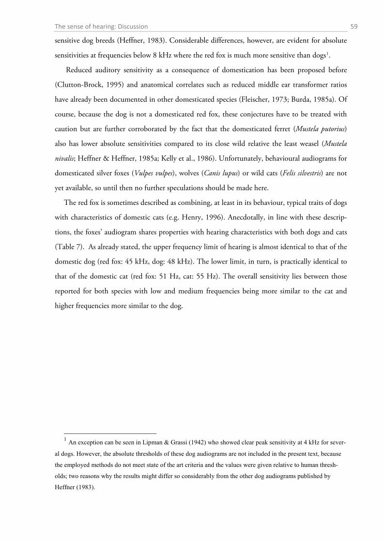
The sense of hearing: Discussion 59
sensitive dog breeds (Heffner, 1983). Considerable differences, however, are evident for absolute
sensitivities at frequencies below 8 kHz where the red fox is much more sensitive than dogs1.
Reduced auditory sensitivity as a consequence of domestication has been proposed before
(Clutton-Brock, 1995) and anatomical correlates such as reduced middle ear transformer ratios
have already been documented in other domesticated species (Fleischer, 1973; Burda, 1985a). Of
course, because the dog is not a domesticated red fox, these conjectures have to be treated with
caution but are further corroborated by the fact that the domesticated ferret (Mustela putorius)
also has lower absolute sensitivities compared to its close wild relative the least weasel (Mustela
nivalis; Heffner & Heffner, 1985a; Kelly et al., 1986). Unfortunately, behavioural audiograms for
domesticated silver foxes (Vulpes vulpes), wolves (Canis lupus) or wild cats (Felis silvestris) are not
yet available, so until then no further speculations should be made here.
The red fox is sometimes described as combining, at least in its behaviour, typical traits of dogs
with characteristics of domestic cats (e.g. Henry, 1996). Anecdotally, in line with these descrip-
tions, the foxes’ audiogram shares properties with hearing characteristics with both dogs and cats
(Table 7). As already stated, the upper frequency limit of hearing is almost identical to that of the
domestic dog (red fox: 45 kHz, dog: 48 kHz). The lower limit, in turn, is practically identical to
that of the domestic cat (red fox: 51 Hz, cat: 55 Hz). The overall sensitivity lies between those
reported for both species with low and medium frequencies being more similar to the cat and
higher frequencies more similar to the dog.
1 An exception can be seen in Lipman & Grassi (1942) who showed clear peak sensitivity at 4 kHz for sever-
al dogs. However, the absolute thresholds of these dog audiograms are not included in the present text, because
the employed methods do not meet state of the art criteria and the values were given relative to human thresh-
olds; two reasons why the results might differ so considerably from the other dog audiograms published by
Heffner (1983).
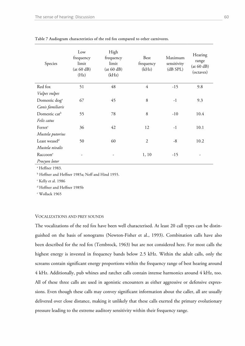
The sense of hearing: Discussion 60
Table 7 Audiogram characteristics of the red fox compared to other carnivores.
Species
Low frequency
limit (at 60 dB)
(Hz)
High frequency
limit (at 60 dB)
(kHz)
Best frequency
(kHz)
Maximum sensitivity (dB SPL)
Hearing range
(at 60 dB) (octaves)
Red fox 51 48 4 -15 9.8 Vulpes vulpes
Domestic doga 67 45 8 -1 9.3 Canis familiaris
Domestic catb 55 78 8 -10 10.4 Felis catus
Ferretc 36 42 12 -1 10.1 Mustela putorius
Least weaseld 50 60 2 -8 10.2 Mustela nivalis
Raccoone - - 1, 10 -15 - Procyon lotor a Heffner 1983.
b Heffner and Heffner 1985a; Neff and Hind 1955. c Kelly et al. 1986
d Heffner and Heffner 1985b e Wollack 1965
VOCALIZATIONS AND PREY SOUNDS
The vocalizations of the red fox have been well characterised. At least 20 call types can be distin-
guished on the basis of sonograms (Newton-Fisher et al., 1993). Combination calls have also
been described for the red fox (Tembrock, 1963) but are not considered here. For most calls the
highest energy is invested in frequency bands below 2.5 kHz. Within the adult calls, only the
screams contain significant energy proportions within the frequency range of best hearing around
4 kHz. Additionally, pub whines and ratchet calls contain intense harmonics around 4 kHz, too.
All of these three calls are used in agonistic encounters as either aggressive or defensive expres-
sions. Even though these calls may convey significant information about the caller, all are usually
delivered over close distance, making it unlikely that these calls exerted the primary evolutionary
pressure leading to the extreme auditory sensitivity within their frequency range.
The sense of hearing: Discussion 61
Red foxes are crepuscular and nocturnal hunters which heavily rely on their auditory system
for localization of prey (Tembrock et al., 1957; Österholm, 1964). It is thus conceivable that
their audiogram reveals special adaptations reflecting enhanced perception of prey sounds. Even
though the red fox is rather a generalist or sometimes even described as an opportunistic feeder, a
considerable proportion of its diet consists of vertebrate prey such as small mammals (in most
reports more than 50% rodents, but see Catling, 1988) and birds (maximum 10-20 %) which are
assumed to be a constant key resource (Harris, 1981; Hockman & Chapman, 1983; Cavallini &
Volpi, 1996; Jankowiak & Tryjanowski, 2013). From these two groups, voles and birds of the
Phasianidae family constitute the main proportions (Lever, 1959; Goszczyński, 1974; Hewson &
Kolb, 1975; Dell'Arte et al., 2007). Red foxes localize sounds most accurately between 3-4 kHz
and this has been proposed to help finding common pheasant-chicks (Phasianus colchicus) by their
flock call which is pitched around 4 kHz (Heinz & Gysel, 1970; Isley & Gysel, 1975). It is strik-
ing that this frequency region of best localization exactly coincides with the highest absolute sen-
sitivity of the red fox. The possibility that the good localization capability might simply be a con-
sequence of the increased perception was already discussed by Isley and Gysel (1975), but seems
unlikely as an explanation for the different localization accuracy in the mid-frequency range as the
intensity of the presented tones was far above threshold (74 ± 4 dB SPL). Thus, it is plausible that
the high hearing sensitivity at 4 kHz aids in finding avian prey over large distances during fox for-
aging bouts. At this point it is tempting to speculate that the good low frequency sensitivity (in
the region around 100 Hz) of the red fox might also be related to the localization of phasanid
prey, since many of these bird species communicate in this frequency range over large distance by
means of drumming displays (Garcia et al., 2012).
Small mammals emit both vocalizations and involuntary sounds during movement and feed-
ing. Both can potentially be exploited by predators, to identify, track, and locate their prey. Rus-
tling noise is broadband but contains most energy in bands at 8-10 kHz and their first harmonics
(Payne, 1971; Konishi, 1973; Marimuthu & Neuweiler, 1987). Even though the ability of the
red fox to localize pure tones is lowest at these frequencies, they can still provide reliable spatial
information, probably enough to allow for increased hunting success at shorter distance (Isley &
Gysel, 1975). In contrast to rustling sounds, the vocalizations of voles and mice are mainly ultra-
sonic between 50-70 kHz (Sewell, 1968). Ultrasound attenuates very quickly and since thresholds
for sounds with frequencies higher than 50 kHz are above 60 dB SPL in the red fox, it seems un-
The sense of hearing: Discussion 62
likely that rodent communications sounds are helpful in prey localization. To sum up, if the high
sensitivity to frequencies around 4 kHz developed in response to the pressure of localizing prey
items, it was most likely helpful in finding avian prey over larger distances rather than rodents in
the grass or below snow cover.
LOW AND HIGH FREQUENCY HEARING
A crucial function of hearing is the ability of localizing sound sources such as prey, mates or pred-
ators. Mammals localize sounds with help of monaural and binaural cues (reviewed in Butler,
1975; Gourevitch, 1980; Heffner & Heffner, 1992b). Monaural (pinna) cues mainly aid in the
vertical localization of sounds and front/back reversals, whereas binaural cues allow for discrimi-
nations in the horizontal plane. Interaural differences are of both temporal nature, arising from
the distance between the ears (interaural time difference, ITD), and spectral nature, through the
shadowing effect of the head and the pinnae (interaural level difference, ILD).
The maximal ITD depends on the size of an animal’s head. Thus, the smaller the head, the
smaller the maximal available ITD. Head size is constrained, but at the same time accurate sound
localization is crucial, hence mammals improved the efficiency of their second sound localization
cue, the ILD. Particularly, it has been suggested that the smaller the mammal, the more it de-
pends on ILD for sound localization (Masterton et al., 1969). High frequencies are better attenu-
ated than low frequencies and larger heads attenuate lower frequencies than smaller heads. As a
consequence, a small mammal that relies on ILD needs to hear frequencies that are high enough
to be effectively shadowed by its tiny head (Heffner & Heffner, 2008a). This relationship is sub-
stantiated by a highly significant negative correlation between the upper limit of hearing and the
functional head size of an animal (time of the sound to travel around the head from one auditory
meatus to the other; Heffner & Heffner, 1981). With a typical functional head size of 320 µs, the
red fox has a predicted high frequency cutoff at 41 kHz (underlying dataset containing 67 species;
from Heffner & Heffner, 2008a). This is only marginally lower than the measured limit of 48
kHz; hence the fox further contributes to the good correlation between interaural distance and
the upper limit of hearing.
Amongst all factors included so far, the low frequency limit of a species has only been shown
to be negatively correlated with the high frequency limit of species (Heffner & Heffner, 2008b).
In general, mammals appear to be split in two groups of low frequency hearing characteristics:
The sense of hearing: Discussion 63
those with normal low frequency hearing and those with extended low frequency hearing
(retained sensitivity below 125 Hz; Heffner et al., 2001). Since hearing of low frequencies is a
common feature of most vertebrates, and only mammals developed high frequency hearing
(> 10 kHz), the latter is believed to be the derived state (Heffner et al., 2001). Not all mammals
have, however, gained (or retained) the ability to hear both very low and very high frequencies.
Amongst “broadband-listeners” are carnivores such as the least weasel (50 Hz-60 kHz) and the
domestic cat (55 Hz-79 kHz). The red fox (51 Hz-48 kHz) might also be assorted to this group.
Proximately, details of inner and middle ear morphology could reveal anatomical similarities of
these species that might be the responsible morphological adaptations contributing to the extend-
ed hearing range (see below). Ultimate reasons for retained low frequency hearing might reside in
the sound localization abilities of red foxes: The localization of a sound takes place mainly on ba-
sis of its high frequency content (Heffner et al., 1995). Therefore, it has been proposed that ani-
mals for which the localization of sound is essential might have given up low frequency hearing
that might detrimentally mask important high frequencies (Heffner et al., 2001). However,
sound localization acuity is outstanding in the domestic cat which also is an auditory hunter that
has retained both high and low frequency sensitivity (Casseday & Neff, 1973; Heffner &
Heffner, 1988a). Obviously, sound localization is even more important for a non-domesticated
auditory predator such as the red fox. Hence it follows that either the extreme absolute sensitivi-
ties in the best frequency range (which, as we remember were also localized best; Isley & Gysel,
1975) or some unknown adaptations of sound localization mechanisms have allowed the red fox
to keep its high sensitivity in the low frequency range.
PHYSIOLOGICAL MEASURES OF HEARING SENSITIVITY
A behavioural audiogram is not the only means of measuring an animal’s hearing sensitivity. Elec-
trophysiological responses to sounds that are recorded at the level of the inner ear (cochlear mi-
crophonic potentials) or the auditory nerve/brainstem (auditory evoked potentials) are often used
to estimate certain characteristics of the audiogram. Peterson et al. (1969) employed cochlear mi-
crophonic potentials in several carnivores including six specimens of the red fox. Figure 1.4-2
compares the mean cochlear microphonic audiogram of these foxes to the behavioural audiogram.
It is obvious that considerable differences exist between the two audiograms with much higher
thresholds in the electrophysiological audiogram and shifted regions of best sensitivity. In contrast
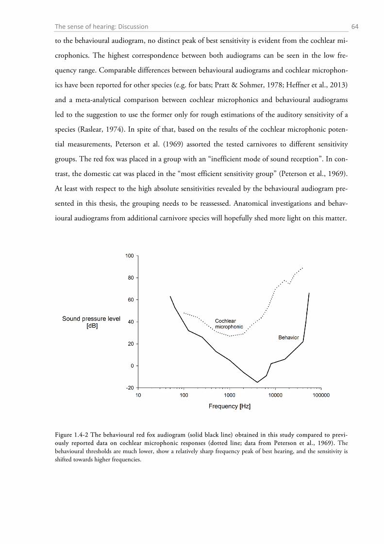
The sense of hearing: Discussion 64
to the behavioural audiogram, no distinct peak of best sensitivity is evident from the cochlear mi-
crophonics. The highest correspondence between both audiograms can be seen in the low fre-
quency range. Comparable differences between behavioural audiograms and cochlear microphon-
ics have been reported for other species (e.g. for bats; Pratt & Sohmer, 1978; Heffner et al., 2013)
and a meta-analytical comparison between cochlear microphonics and behavioural audiograms
led to the suggestion to use the former only for rough estimations of the auditory sensitivity of a
species (Raslear, 1974). In spite of that, based on the results of the cochlear microphonic poten-
tial measurements, Peterson et al. (1969) assorted the tested carnivores to different sensitivity
groups. The red fox was placed in a group with an “inefficient mode of sound reception”. In con-
trast, the domestic cat was placed in the “most efficient sensitivity group” (Peterson et al., 1969).
At least with respect to the high absolute sensitivities revealed by the behavioural audiogram pre-
sented in this thesis, the grouping needs to be reassessed. Anatomical investigations and behav-
ioural audiograms from additional carnivore species will hopefully shed more light on this matter.
Figure 1.4-2 The behavioural red fox audiogram (solid black line) obtained in this study compared to previ-ously reported data on cochlear microphonic responses (dotted line; data from Peterson et al., 1969). The behavioural thresholds are much lower, show a relatively sharp frequency peak of best hearing, and the sensitivity is shifted towards higher frequencies.
The sense of hearing: Discussion 65
1.4.2 Anatomy
THE RED FOX EAR IN COMPARATIVE CONTEXT OF MAMMALIAN EARS
In the following, I will discuss specific aspects of the red fox ear morphology in comparison to
findings in other mammals. The plethora of data that I have collected renders a detailed discus-
sion of all parameters impossible. Therefore, I will dwell on selected characteristics only.
Outer and middle ear
The pinna of mammals is a highly complicated acoustical structure; the essential parameters are
hard to put into numbers. Therefore, I only determined a very rough variable, the height to width
ratio. I did not collect more variables as the effect of the pinna has been shown to be almost ne-
glectable when it comes to overall sensitivity of the auditory system (Heffner, 1983; Coleman &
Colbert, 2010). The ratio might prove useful in a large comparative context (all carnivores), but
since no such dataset exists at the moment, any inference on basis of pinna morphology would be
mere speculation.
The middle ear of the red fox is of the “transitional or intermediate type” defined by Fleischer
(1973, 1978), which is also found in other carnivores such as the cat or the harbour seal
(overview in Rosowski, 1992). The malleus is firmly but only ligamentously attached to the tym-
panic bone. It does not possess an orbicular apophysis, but only a short anterior process and a
reduced transversal lamina. The manubrium forms an angle of approximately 45° to the anatomi-
cal axis of ossicular rotation. The malleus is about twice the size of the incus. Ears of the interme-
diate type are characterised by medium stiffness which is supposed to make them suitable to re-
spond over a wide range of frequencies but not in the extremely low and high frequencies. The
audiogram of the red fox substantiates this prediction: the red fox is less sensitive in the low fre-
quency range than e.g. primates and subterranean mammals that possess middle ears of the “freely
mobile type”, and it is also less sensitive in the high frequency range compared to small rodents or
bats that possess the stiff “microtype” middle ear.
The size of the auditory bulla is related to the sensitivity in the low frequency range. Animals
adapted to hear very low frequencies, such as the kangaroo rat, possess extremely hypertrophied
bullae (Webster, 1962; Webster & Webster, 1972). The bulla of the cat is approximately 25%
smaller than that of the red fox (Lynch et al., 1981), but this does not seem to have an effect on
The sense of hearing: Discussion 66
the low frequency hearing. With respect to the feline bulla (Keen & Grobbelaar, 1941), it is in-
teresting to know that they are characterised by a septum which divides the bulla. This kind of
separation has been related to the 4 kHz-ditch in the cat audiogram. The fact that the fox does
not have such a pronounced partition fits well with the high sensitivity at 4 kHz.
Even though we know that the middle ear does not act as an ideal transformer it is still inter-
esting to compare the theoretical middle ear transmission properties of a newly studied species to
known values of other well studied animals.
The middle ear impedance transformer ratio (ITR) of the red fox (0.0072) is slightly smaller
(i.e. more efficient) than the ITR of the cat (0.0079; cf. Table A9 appendix). This corresponds
well to the higher absolute sensitivity found in the red fox audiogram.
The ossicle mass is discussed to have most influence on high frequency middle ear transmis-
sion (Dallos, 1973; Manley & Johnstone, 1974; but see e.g. Overstreet & Ruggero, 2002 for a
contradicting view). Therefore, I would expect lower ossicle mass in the cat compared to the dog
and the red fox. Indeed, the cat ossicles weigh less than those of the adult red fox specimens in my
sample and those reported in Nummela (1995), which fits to the better higher frequency hearing
in the cat. In contrast, the ossicles of the dog are considerably heavier, although the upper fre-
quency limit is identical to the red fox. Thus, the general trend of lower high frequency limits is
supported by those numbers, but it is evident that the body mass as an additional component has
to be taken into account (Hunt & Korth, 1980). The relationship between body mass and ossicle
weight is also evident in the development of the red fox middle ear reported here. Since the mass
changes were not accompanied by linear changes of ossicular dimensions, the influence of ontog-
eny on hearing is not straightforward to predict on a morphological basis of middle ear parame-
ters.
Inner ear
Before I will start discussing some of the interesting observations on the inner ear of the red fox in
a comparative context, some remarks about the general quality of the material and the procedure
of cochlear sectioning seem to be appropriate. Establishing a histological procedure for sectioning
of the cochlea is by no means a trivial endeavour. The unique combination of very delicate struc-
tures embedded within the hardest bone of the body imposes such special requirements that it is
impossible to gather good results quickly, especially in larger animals where the time needed to
The sense of hearing: Discussion 67
adapt existing procedures to a new species can very well take several months or even years (Wever
et al., 1971). Additionally, even when the sectioning procedure is running, the quality of the ma-
terial often diminishes the results, as specimens of non-laboratory species are mostly simply im-
mersion-fixed, because perfusion in the field is extremely difficult to accomplish (although not
impossible, see Manger et al., 2009 for an impressive example). My red fox specimens were well
preserved but not perfused and therefore the quality of inner ear sections could not be expected to
be outstanding. I optimized the procedure as much as I could (cf. Figure 1.2-6) and yielded good
results. However, the quality differed between individuals and thus on many sections not all pa-
rameters could be measured. This was especially problematic for the determination of hair cell
lengths, where the presented figures are based on small numbers. This should be kept in mind
during the discussion of the functional consequences below.
Some of the morphological parameters of the red fox inner ear are shown in comparison to
published figures of other carnivores in Table A9 (appendix). With 3.2 turns, the red fox cochlea
is in this respect similar to the dog (3.25 turns; Gray, 1907; Keen, 1939; Le & Keithley, 2007)
and the cat (3 turns; Gray, 1907; Keen, 1939). Three or less turns might be a characteristic of the
Felidae irrespective of body size, as the tiger and jaguar have 2.75 turns (Burda et al., 1984).
Thus, even though BM length is closely correlated with body size (see below), the coiling of the
cochlea seems to be decoupled from this development. The number of cochlear turns has been
related to the hearing range in octaves (Echteler et al., 1994). Given the small differences in the
number of turns between cat, dog, and the red fox, the small difference of (less than) one octave
in their hearing ranges supports the relationship.
Compared to the domestic cat, the basilar membrane (BM) of the red fox is slightly longer
(cat: 22-25 mm; Retzius, 1884; Schuknecht, 1953; West & Harrison, 1973; Cabezudo, 1978;
West, 1985; Sato et al., 1999)2. This fits well to the generally observed positive correlation be-
tween body weight and BM length (Vater & Kössl, 2011), as the red fox is larger than the cat.
The values reported for the BM length of the dog are within the same range as those reported for
the cat (22-24.5 mm; Schuknecht et al., 1965; Igarashi et al., 1972; Mair, 1976), seemingly con-
tradicting the BM-body size relationship, as the used dog breeds (Beagle, Dalmatian) considerably
outweigh the cat, and it has been shown that at least middle ear morphological parameters are
closely related to body size in different dog breeds (Heffner, 1983).
2 Note that unpublished measurements by Burda suggest considerably longer cat BM lengths of 27-28 mm
(see below)
The sense of hearing: Discussion 68
It is for this reason highly interesting to note, that for both dog (Branis & Burda, 1985) and
cat (Burda, unpublished) longer BM lengths have been found than those published in other stud-
ies. The dissent may emerge from the fact that different methods were used for the assessment.
Burda (unpublished) and Branis & Burda (1985) used the method of surface specimens which
has also been employed in the current study on the red fox. All other studies either used serial sec-
tions or mid-modiolar sections and the method of Guild (1921), both of which might be prone
to underestimation of the actual BM length (Greenwood, 1990). To my knowledge, the only
other study which used surface specimens of the cat cochlea to estimate BM length was the study
by Liberman (1982) who reported lengths between 23 and 26.7 mm. A longer BM length in the
cat than in the fox would fit the larger hearing range of the former, while a longer BM in the dog
might be simply related to the relationship to body size. Even with a BM length comparable to
the red fox, the cat probably deviates from the BM–body size relationship, maybe as a result of
special sensory adaptations as has already been conjectured for the cat cochlea by Hemilä et al.
(1995). Again fitting to the correlation with body size are the reported BM lengths for the jaguar
(33.3 mm) and the tiger (35.5 mm; Burda et al., 1984).
A longer BM provides additional surface area to accommodate more sensory hair cells. The to-
tal number of IHCs in the red fox matches almost exactly the number that has been found in the
cat (red fox: 2,757, cat: 2,723; Burda, unpublished), while it is considerably higher than the
number of IHCs reported for the dog (2,603; Branis & Burda, 1985). On the other hand, the
number of OHCs is identical between red fox and dog, while being lower in the cat (red fox:
10,503, dog: 10,548, cat: 10,105; Branis & Burda, 1985; Burda, unpublished). Thus, even in
inner ear morphology we find a reflection of the cani-feline properties of the red fox hearing sys-
tem that we already discussed for the audiogram above.
How do these hair cell numbers relate to hearing function? An increased density of sensory
hair cells as observed for the IHCs in the red fox and cat compared to the dog, might either lead
to increased frequency and amplitude discrimination abilities or to increased sensitivity of the au-
ditory system (Ehret & Frankenreiter, 1977; Burda & Voldřich, 1980; Liberman, 1982; Burda,
1985b). We do not know anything about frequency discrimination in the red fox, but it is strik-
ing that the audiogram of red fox and cat are both characterised by a higher number of IHCs and
a distinctly higher absolute sensitivity than the one of the dog (cf. Figure 1.4-1).
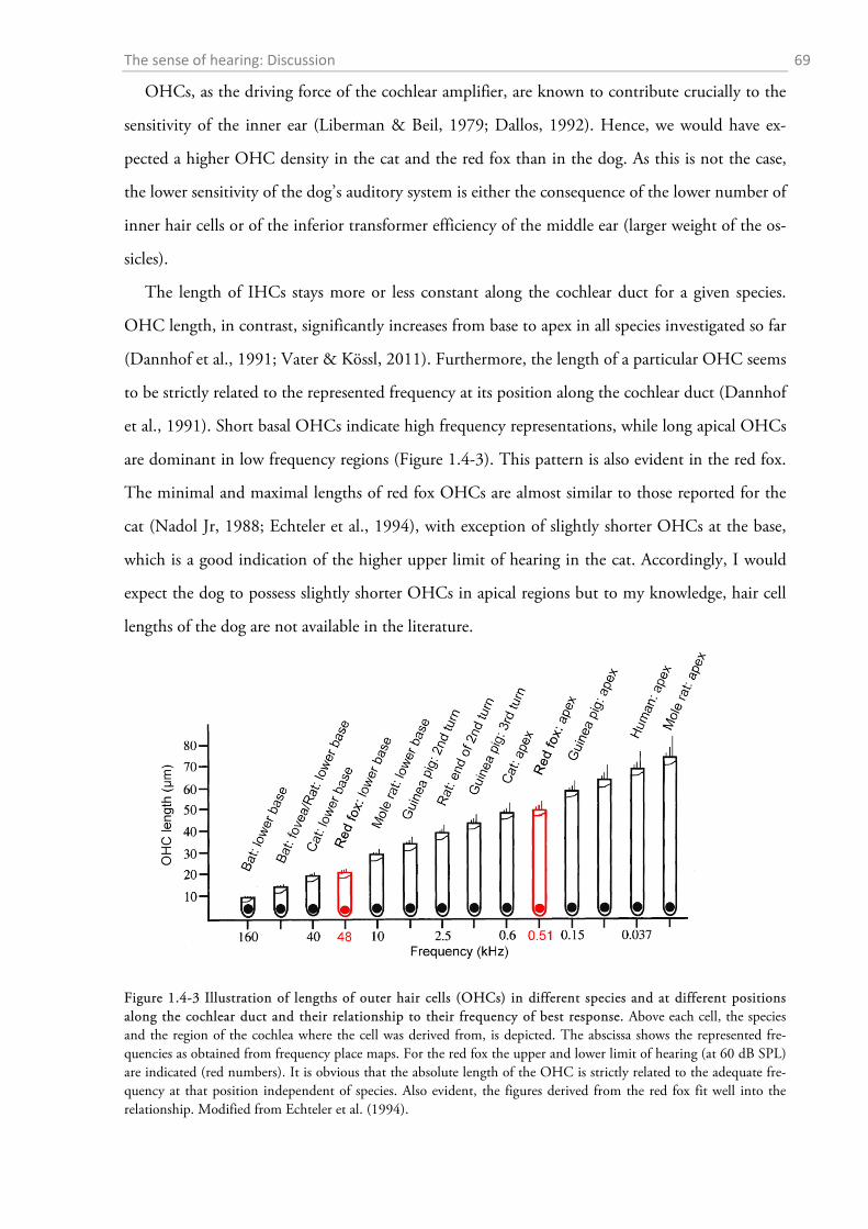
The sense of hearing: Discussion 69
OHCs, as the driving force of the cochlear amplifier, are known to contribute crucially to the
sensitivity of the inner ear (Liberman & Beil, 1979; Dallos, 1992). Hence, we would have ex-
pected a higher OHC density in the cat and the red fox than in the dog. As this is not the case,
the lower sensitivity of the dog’s auditory system is either the consequence of the lower number of
inner hair cells or of the inferior transformer efficiency of the middle ear (larger weight of the os-
sicles).
The length of IHCs stays more or less constant along the cochlear duct for a given species.
OHC length, in contrast, significantly increases from base to apex in all species investigated so far
(Dannhof et al., 1991; Vater & Kössl, 2011). Furthermore, the length of a particular OHC seems
to be strictly related to the represented frequency at its position along the cochlear duct (Dannhof
et al., 1991). Short basal OHCs indicate high frequency representations, while long apical OHCs
are dominant in low frequency regions (Figure 1.4-3). This pattern is also evident in the red fox.
The minimal and maximal lengths of red fox OHCs are almost similar to those reported for the
cat (Nadol Jr, 1988; Echteler et al., 1994), with exception of slightly shorter OHCs at the base,
which is a good indication of the higher upper limit of hearing in the cat. Accordingly, I would
expect the dog to possess slightly shorter OHCs in apical regions but to my knowledge, hair cell
lengths of the dog are not available in the literature.
Figure 1.4-3 Illustration of lengths of outer hair cells (OHCs) in different species and at different positions along the cochlear duct and their relationship to their frequency of best response. Above each cell, the species and the region of the cochlea where the cell was derived from, is depicted. The abscissa shows the represented fre-quencies as obtained from frequency place maps. For the red fox the upper and lower limit of hearing (at 60 dB SPL) are indicated (red numbers). It is obvious that the absolute length of the OHC is strictly related to the adequate fre-quency at that position independent of species. Also evident, the figures derived from the red fox fit well into the relationship. Modified from Echteler et al. (1994).
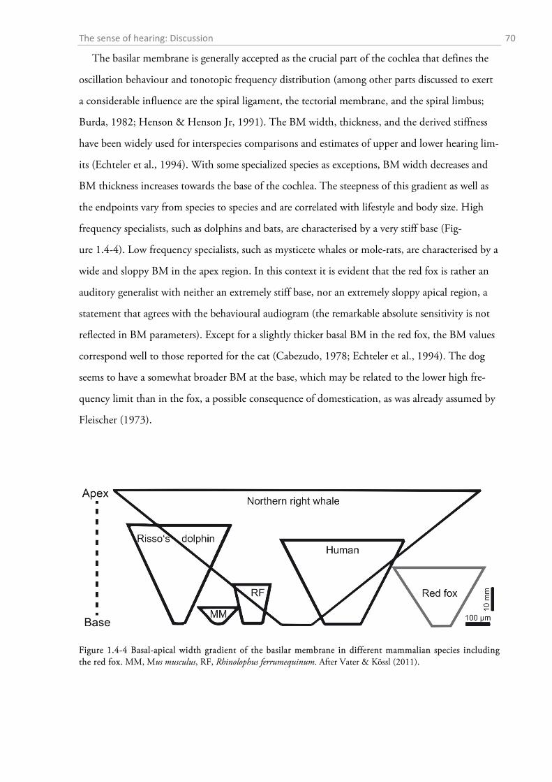
The sense of hearing: Discussion 70
The basilar membrane is generally accepted as the crucial part of the cochlea that defines the
oscillation behaviour and tonotopic frequency distribution (among other parts discussed to exert
a considerable influence are the spiral ligament, the tectorial membrane, and the spiral limbus;
Burda, 1982; Henson & Henson Jr, 1991). The BM width, thickness, and the derived stiffness
have been widely used for interspecies comparisons and estimates of upper and lower hearing lim-
its (Echteler et al., 1994). With some specialized species as exceptions, BM width decreases and
BM thickness increases towards the base of the cochlea. The steepness of this gradient as well as
the endpoints vary from species to species and are correlated with lifestyle and body size. High
frequency specialists, such as dolphins and bats, are characterised by a very stiff base (Fig-
ure 1.4-4). Low frequency specialists, such as mysticete whales or mole-rats, are characterised by a
wide and sloppy BM in the apex region. In this context it is evident that the red fox is rather an
auditory generalist with neither an extremely stiff base, nor an extremely sloppy apical region, a
statement that agrees with the behavioural audiogram (the remarkable absolute sensitivity is not
reflected in BM parameters). Except for a slightly thicker basal BM in the red fox, the BM values
correspond well to those reported for the cat (Cabezudo, 1978; Echteler et al., 1994). The dog
seems to have a somewhat broader BM at the base, which may be related to the lower high fre-
quency limit than in the fox, a possible consequence of domestication, as was already assumed by
Fleischer (1973).
Figure 1.4-4 Basal-apical width gradient of the basilar membrane in different mammalian species including the red fox. MM, Mus musculus, RF, Rhinolophus ferrumequinum. After Vater & Kössl (2011).
The sense of hearing: Discussion 71
The basal stiffness values of the red fox are a bit conspicuous, as they are within a range typical for
animals with much higher upper hearing limits (fox: 0.015, mouse: 0.013, horseshoe bat: 0.013,
dolphin: 0.014; Echteler et al., 1994). Since I performed the calculation of the stiffness with BM
properties found at the very end of the hook region, it might well be that the cochlear partition is
not functional in this regions. The BM width decreased considerably in this region and if non-
functional anymore, this might have led to a slight overestimation of basal stiffness as a functional
variable of red fox hearing. For future calculations of stiffness it is therefore warranted to take the
mean values between the hook and first half-turn as the basal BM values of the red fox.
To conclude, the morphology of the red fox inner ear resembles in many parts those of the cat
and the dog. Even though direct causality cannot be drawn, the finding is supportive of the con-
spicuous “sensory-hybridization” that was already suggested by the behavioural audiogram.
COULD I HAVE PREDICTED THE RED FOX AUDIOGRAM FROM THE ANATOMY?
The unique set of detailed anatomical and behavioural data that I have presented within this
chapter creates the opportunity to test several of the published correlations between ear morphol-
ogy and auditory function and thereupon based models and predictions. The goal of this section
will be to determine those anatomical parameters that allow the most accurate reproduction of
the audiogram of the red fox. For the predictions, I take only morphological parameters of the ear
into account but none of the parameters that I obtained from the actual behavioural audiogram.
To keep it simple, I will break down the behavioural audiogram into three audiometric variables
that have been proven useful in comparative studies of the audiograms in other species (e.g.
Rosowski & Graybeal, 1991; Coleman & Colbert, 2010). These variables are:
1. the high frequency limit (at 60 dB SPL and 30 dB SPL above best threshold)
2. the low frequency limit (at 60 dB SPL and 30 dB SPL above best threshold)
3. the frequency of best sensitivity
The sense of hearing: Discussion 72
(1) High frequency limit
According to Rosowski (1992), the high frequency limit (at 30 dB SPL above best threshold) of
every mammal can be approximately predicted by three different equations (eq.):
𝐹𝑚𝑚𝑚 = 110 × 𝑇𝑇−0.37 (eq. 1)
(TM = area of the tympanic membrane; mm²)
𝐹𝑚𝑚𝑚 = 34 × 𝑂𝑂−0.4 (eq. 2)
(OW = area of oval window; mm²)
𝐹𝑚𝑚𝑚 = 391 × 𝐵𝑇𝐵−0.85 (eq. 3)
(BMl = length of basilar membrane; mm)
The predicted upper frequency limits (at 30 dB above best threshold) for the red fox are 29.5
kHz (according to eq. 1), 26.9 kHz (eq. 2), and 24.7 kHz (eq. 3), resulting in a mean predicted
upper frequency limit of 27 kHz (30 dB SPL above threshold).
West (1985) determined the following equation for estimating the high frequency limit at 60 dB
SPL:
𝐹𝑚𝑚𝑚 = 10(2.42−0.994×log (𝐵𝑇𝐵𝐶𝑇 ) × 1000 (eq. 4)
(at 60 dB SPL); (CT = number of cochlear turns)
which translates into 33 kHz when taking the CT and BMl of the red fox into account.
(2) Low frequency limit
According to Rosowski (1992), the predicted low frequency limit (at 30 dB SPL above best threshold) is:
𝐹𝑚𝑚𝑚 = 15 × 𝑇𝑇−1.1 (eq. 5)
(TM = area of the tympanic membrane; mm²)
𝐹𝑚𝑚𝑚 = 0.4 × 𝑂𝑂−1.1 (eq. 6)
(OW = area of oval window; mm²)
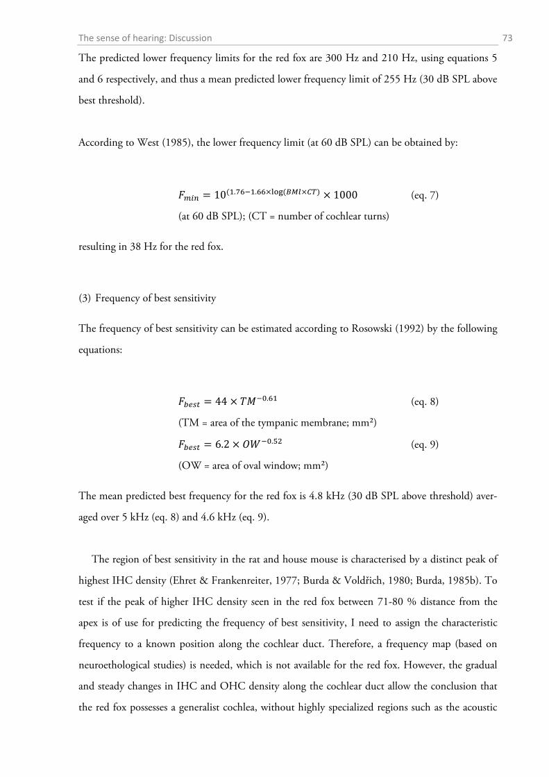
The sense of hearing: Discussion 73
The predicted lower frequency limits for the red fox are 300 Hz and 210 Hz, using equations 5
and 6 respectively, and thus a mean predicted lower frequency limit of 255 Hz (30 dB SPL above
best threshold).
According to West (1985), the lower frequency limit (at 60 dB SPL) can be obtained by:
𝐹𝑚𝑚𝑚 = 10(1.76−1.66×log (𝐵𝐵𝑙×𝐶𝐶) × 1000 (eq. 7)
(at 60 dB SPL); (CT = number of cochlear turns)
resulting in 38 Hz for the red fox.
(3) Frequency of best sensitivity
The frequency of best sensitivity can be estimated according to Rosowski (1992) by the following
equations:
𝐹𝑏𝑏𝑏𝑏 = 44 × 𝑇𝑇−0.61 (eq. 8)
(TM = area of the tympanic membrane; mm²)
𝐹𝑏𝑏𝑏𝑏 = 6.2 × 𝑂𝑂−0.52 (eq. 9)
(OW = area of oval window; mm²)
The mean predicted best frequency for the red fox is 4.8 kHz (30 dB SPL above threshold) aver-
aged over 5 kHz (eq. 8) and 4.6 kHz (eq. 9).
The region of best sensitivity in the rat and house mouse is characterised by a distinct peak of
highest IHC density (Ehret & Frankenreiter, 1977; Burda & Voldřich, 1980; Burda, 1985b). To
test if the peak of higher IHC density seen in the red fox between 71-80 % distance from the
apex is of use for predicting the frequency of best sensitivity, I need to assign the characteristic
frequency to a known position along the cochlear duct. Therefore, a frequency map (based on
neuroethological studies) is needed, which is not available for the red fox. However, the gradual
and steady changes in IHC and OHC density along the cochlear duct allow the conclusion that
the red fox possesses a generalist cochlea, without highly specialized regions such as the acoustic

The sense of hearing: Discussion 74
foveae reported from bats (Bruns & Schmieszek, 1980) and mole-rats (Müller et al., 1992).
Therefore, it is possible to estimate a cochlea frequency map by means of an equation developed
by Greenwood (1961, 1974, 1990):
𝑓 = 𝐴 × (10𝑚𝑚 − 𝑘) (eq. 10)
where f is the frequency in Hz, A is a scale factor that is dependent on the high frequency limit
(60 dB SPL), x is the normalized distance from the apex, a is describing the steepness of the map,
and k a constant that serves a better fit for the low frequency data. The constants differ slightly
between species (overview in LePage, 2003). The predictive power of the equation was validated
in the cat by Liberman (1982) by means of horseradish peroxidase injected into the cochlear nu-
cleus at positions associated with characterised frequencies. Fay (1992) has further simplified and
validated equation 10, and ultimately developed the following formula to predict the frequency
represented at a specific position p (as a distance (in mm) from the base):
𝑝 = (1 − �𝐵𝑙𝑔10 �𝑓𝐻𝐻
0.008𝐹𝑚𝑚𝑚� + 1�)/2.1)) (eq. 11)
where Fmax is the high frequency threshold at 60 dB SPL. Using equation 11 and the predicted
high frequency cutoff (eq. 4), I created a position-frequency map from which the represented fre-
quency at the distance 75% away from the apex can be read. The resultant frequency for the posi-
tion of highest IHC density was 9.5 kHz (eq. 11, Fmax = 33 kHz).
The position frequency map for the prediction is shown in Figure 1.4-5.
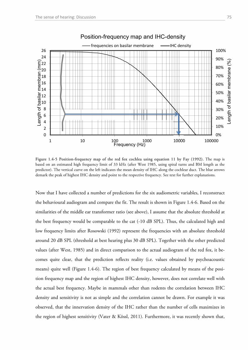
The sense of hearing: Discussion 75
Figure 1.4-5 Position-frequency map of the red fox cochlea using equation 11 by Fay (1992). The map is based on an estimated high frequency limit of 33 kHz (after West 1985, using spiral turns and BM length as the predictor). The vertical curve on the left indicates the mean density of IHC along the cochlear duct. The blue arrows demark the peak of highest IHC density and point to the respective frequency. See text for further explanations.
Now that I have collected a number of predictions for the six audiometric variables, I reconstruct
the behavioural audiogram and compare the fit. The result is shown in Figure 1.4-6. Based on the
similarities of the middle ear transformer ratio (see above), I assume that the absolute threshold at
the best frequency would be comparable to the cat (-10 dB SPL). Thus, the calculated high and
low frequency limits after Rosowski (1992) represent the frequencies with an absolute threshold
around 20 dB SPL (threshold at best hearing plus 30 dB SPL). Together with the other predicted
values (after West, 1985) and in direct comparison to the actual audiogram of the red fox, it be-
comes quite clear, that the prediction reflects reality (i.e. values obtained by psychoacoustic
means) quite well (Figure 1.4-6). The region of best frequency calculated by means of the posi-
tion frequency map and the region of highest IHC density, however, does not correlate well with
the actual best frequency. Maybe in mammals other than rodents the correlation between IHC
density and sensitivity is not as simple and the correlation cannot be drawn. For example it was
observed, that the innervation density of the IHC rather than the number of cells maximizes in
the region of highest sensitivity (Vater & Kössl, 2011). Furthermore, it was recently shown that,
0%
10%
20%
30%
40%
50%
60%
70%
80%
90%
100%80.0100.0120.0140.0160.0180.0200.0220.0240.0260.0280.0300.0320.0340.0360.0380.0400.0420.0440.0
02468
101214161820222426
1 10 100 1000 10000 100000
Leng
th o
f bas
ilar m
embr
ane
(%)
Leng
th o
f bas
ilar m
embr
an (m
m)
Frequency (Hz)
Position-frequency map and IHC-density frequencies on basilar membrane IHC density
The sense of hearing: Discussion 76
in the chinchilla, IHC loss of up to 80% is not accompanied by a corresponding loss auf auditory
sensitivity (Lobarinas et al., 2013). It is also possible, that the position frequency map is not fit-
ting the real distribution on the red fox cochlea. The function by Greenwood (1990) requires
species-specific parameters which have only been determined for a handful of species (LePage,
2003). The integration constant of -1 for example, which is assumed in the formula by Fay
(1992) (eq. 11), may not be applicable to every species. An absence of functional correlation be-
tween IHC density and best sensitivity is further corroborated when we apply the above described
relationship between OHC length and best resonance frequency to estimate the position of 4 kHz
in the red fox cochlea. Dannhof (1991) reported an OHC length of 36 µm at the position of 4
kHz. In the red fox, outer hair cells of 36 µm length are found in the region of the fifth half-turn,
roughly at a distance 19 mm away from the base, or around 25 % away from the apex. As a con-
clusion, the peak density of IHCs 75 % away from the apex is not related to higher sensitivity but
rather to increased frequency and amplitude discrimination abilities as already discussed above.
The predicted audiogram is slightly shifted towards lower frequencies, except for the frequen-
cy of best hearing. As the prediction is mostly based on middle ear data (except for BM length), it
does not take into account the important influence that has been proposed for the cochlea on
high frequency hearing (Ruggero & Temchin, 2002, 2003). It might well be that the cochlea of
the fox bears some functional adaptations that reduce the impedance at higher frequencies which
would lead to an extended frequency range. With the hair cell data and gross cochlear dimensions
collected in the current study, such effects are hardly predicted but obtaining a transfer function
for the red fox would be an interesting topic for further research.
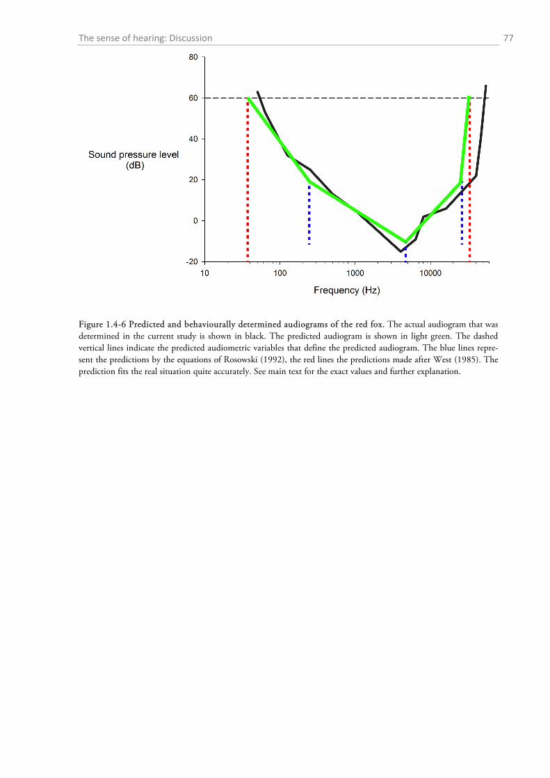
The sense of hearing: Discussion 77
Figure 1.4-6 Predicted and behaviourally determined audiograms of the red fox. The actual audiogram that was determined in the current study is shown in black. The predicted audiogram is shown in light green. The dashed vertical lines indicate the predicted audiometric variables that define the predicted audiogram. The blue lines repre-sent the predictions by the equations of Rosowski (1992), the red lines the predictions made after West (1985). The prediction fits the real situation quite accurately. See main text for the exact values and further explanation.
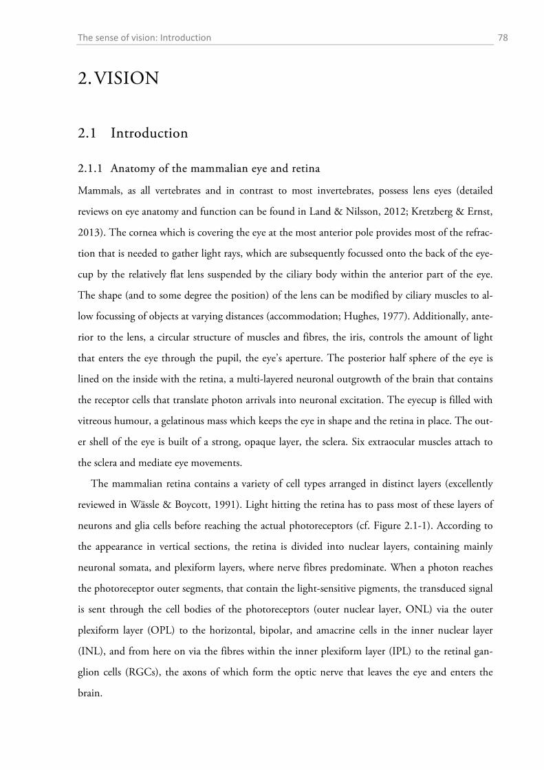
The sense of vision: Introduction 78
2. VISION
2.1 Introduction
2.1.1 Anatomy of the mammalian eye and retina
Mammals, as all vertebrates and in contrast to most invertebrates, possess lens eyes (detailed
reviews on eye anatomy and function can be found in Land & Nilsson, 2012; Kretzberg & Ernst,
2013). The cornea which is covering the eye at the most anterior pole provides most of the refrac-
tion that is needed to gather light rays, which are subsequently focussed onto the back of the eye-
cup by the relatively flat lens suspended by the ciliary body within the anterior part of the eye.
The shape (and to some degree the position) of the lens can be modified by ciliary muscles to al-
low focussing of objects at varying distances (accommodation; Hughes, 1977). Additionally, ante-
rior to the lens, a circular structure of muscles and fibres, the iris, controls the amount of light
that enters the eye through the pupil, the eye’s aperture. The posterior half sphere of the eye is
lined on the inside with the retina, a multi-layered neuronal outgrowth of the brain that contains
the receptor cells that translate photon arrivals into neuronal excitation. The eyecup is filled with
vitreous humour, a gelatinous mass which keeps the eye in shape and the retina in place. The out-
er shell of the eye is built of a strong, opaque layer, the sclera. Six extraocular muscles attach to
the sclera and mediate eye movements.
The mammalian retina contains a variety of cell types arranged in distinct layers (excellently
reviewed in Wässle & Boycott, 1991). Light hitting the retina has to pass most of these layers of
neurons and glia cells before reaching the actual photoreceptors (cf. Figure 2.1-1). According to
the appearance in vertical sections, the retina is divided into nuclear layers, containing mainly
neuronal somata, and plexiform layers, where nerve fibres predominate. When a photon reaches
the photoreceptor outer segments, that contain the light-sensitive pigments, the transduced signal
is sent through the cell bodies of the photoreceptors (outer nuclear layer, ONL) via the outer
plexiform layer (OPL) to the horizontal, bipolar, and amacrine cells in the inner nuclear layer
(INL), and from here on via the fibres within the inner plexiform layer (IPL) to the retinal gan-
glion cells (RGCs), the axons of which form the optic nerve that leaves the eye and enters the
brain.
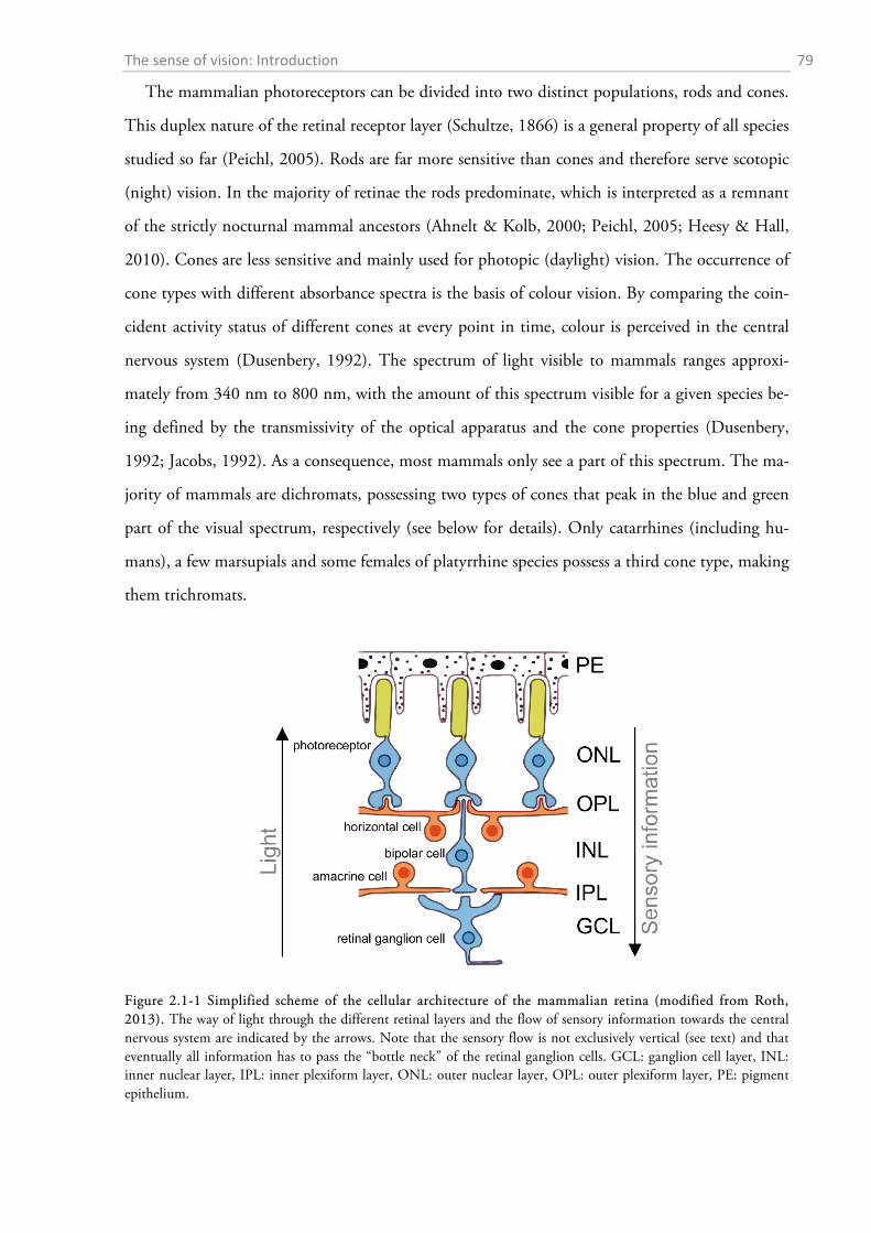
The sense of vision: Introduction 79
The mammalian photoreceptors can be divided into two distinct populations, rods and cones.
This duplex nature of the retinal receptor layer (Schultze, 1866) is a general property of all species
studied so far (Peichl, 2005). Rods are far more sensitive than cones and therefore serve scotopic
(night) vision. In the majority of retinae the rods predominate, which is interpreted as a remnant
of the strictly nocturnal mammal ancestors (Ahnelt & Kolb, 2000; Peichl, 2005; Heesy & Hall,
2010). Cones are less sensitive and mainly used for photopic (daylight) vision. The occurrence of
cone types with different absorbance spectra is the basis of colour vision. By comparing the coin-
cident activity status of different cones at every point in time, colour is perceived in the central
nervous system (Dusenbery, 1992). The spectrum of light visible to mammals ranges approxi-
mately from 340 nm to 800 nm, with the amount of this spectrum visible for a given species be-
ing defined by the transmissivity of the optical apparatus and the cone properties (Dusenbery,
1992; Jacobs, 1992). As a consequence, most mammals only see a part of this spectrum. The ma-
jority of mammals are dichromats, possessing two types of cones that peak in the blue and green
part of the visual spectrum, respectively (see below for details). Only catarrhines (including hu-
mans), a few marsupials and some females of platyrrhine species possess a third cone type, making
them trichromats.
Figure 2.1-1 Simplified scheme of the cellular architecture of the mammalian retina (modified from Roth, 2013). The way of light through the different retinal layers and the flow of sensory information towards the central nervous system are indicated by the arrows. Note that the sensory flow is not exclusively vertical (see text) and that eventually all information has to pass the “bottle neck” of the retinal ganglion cells. GCL: ganglion cell layer, INL: inner nuclear layer, IPL: inner plexiform layer, ONL: outer nuclear layer, OPL: outer plexiform layer, PE: pigment epithelium.
The sense of vision: Introduction 80
2.1.2 Receptor properties and densities
Every visual system has to deal with a trade-off between spatial resolution and sensitivity (Land &
Nilsson, 2012). Enhancing one domain goes along with reduction in the other, so within the
mammalian retina the two types of photoreceptors are specialized to fulfil mainly one of both
tasks each. The rod system provides high sensitivity, both intrinsically through rod properties and
through spatial integration, while the cone system is not only responsible for colour vision but
also for providing maximal visual acuity (spatial resolution).
The receptor mosaic of the retina is specialized to optimize the visual perception within the
species’ habitat, diurnal rhythm and feeding strategy. Nocturnal and crepuscular mammals pos-
sess mainly rods, while the proportion of cones increases with the diurnality of the species (Peichl,
2005). The lowest mammalian rod proportions of less than 10 % have been found in the diurnal
ground squirrel and the tree shrew (West & Dowling, 1975; Müller & Peichl, 1989; Kryger et
al., 1998). In line with this general rule of thumb, fissiped carnivores possess rod dominated reti-
nae (Ahnelt & Kolb, 2000). For example in the cat, the absolute number of rods outnumbers the
cones by a factor of at least 10 and up to 100, depending on the position within the retina
(Steinberg et al., 1973). Although rather spectacular adaptations of the cellular architecture exist
(cf. Solovei et al., 2009) we do not distinguish between different types of rods.
In general, rod and cone photosensitivity is based on the protein opsin linked to a light sensi-
tive chromophore, the retinal (Hunt & Peichl, 2014). Rhodopsin, the visual pigment of rods,
absorbs maximally in the blue-green range around 500 nm in all species (Jacobs, 1993; however,
the peak sensitivity differs slightly between species, Kelber et al., 2003). Small changes in the
amino acid composition of the opsin can shift the absorption maximum of the visual pigment. By
this means, evolution has produced four different classes of cone pigments with peaks in the ul-
traviolet (360 nm; short wavelength-sensitive type 1, SWS1), blue (400-470 nm, SWS2), green-
yellow (480-530 nm; medium wavelength-sensitive, MWS), and red (570 nm; long wavelength-
sensitive, LWS) part of the visual spectrum (Hunt & Peichl, 2014). Only two of these classes
have been retained by extant mammals: the LWS class and one of the SWS classes (SWS2 in
monotremes, SWS1 in all other mammals; reviewed in Davies et al., 2012). Mammalian tri-
chromacy is the result of a de novo duplication of the LWS class opsin, leading to two types of L
pigments which are then commonly referred to as M (530 nm, green) and L (560 nm, red) opsins
(Jacobs et al., 1996; Dulai et al., 1999). All other mammals possess a set of S and M/L cones, al-
The sense of vision: Introduction 81
lowing them dichromatic colour vision (Peichl et al., 2001). In some species even cones express-
ing both S and L opsins occur or even predominate (e.g. Lukáts et al., 2002; reviewed in Lukáts
et al., 2005). Aquatic mammals (including aquatic carnivores) are characterised by a secondary
loss of S cones (Peichl & Moutairou, 1998; Peichl et al., 2001), as are a few strictly nocturnal ter-
restrial mammals (e.g. the racoon, Jacobs & Deegan, 1992; reviewed in Szél et al., 1996).
In most species the photoreceptors show specific density gradients across the retina, and this is
believed to reflect the properties of the environment relevant to each species (Hughes, 1977; Szél
et al., 1996; Peichl, 2005; Ahnelt et al., 2006; Schiviz et al., 2008; Temple, 2011). Primates for
instance possess a fovea, a central depression and region of cone peak density, responsible for
sharp central colour vision. Even though most mammals do not have a fovea, they possess a re-
gion of higher receptor density, slightly inaccurately coined as the central area, or area centralis
(Müller, 1861; Hughes, 1977). In addition, many species are characterised by a horizontal medial
stripe of higher photoreceptor density, the visual streak. Broadly speaking, most mammals possess
this centroperipheral density gradient of photoreceptors. In the majority of species, both S and
M/L cones follow this pattern, the M/L cones being the vast majority outnumbering the S cones
approximately ten times (Peichl, 2005). In several species, however, the pattern of S cones seems
to be decoupled from the M/L cone distribution (Peichl, 2005). This is particularly obvious in
several Mus species where the S cones predominate the ventral retina, while M/L cones prevail in
the dorsal part (Szél et al., 1994). A closely related pattern with high ventral S cone density was
observed in several carnivores, such as cat, tiger, and lion (Linberg et al., 2001; Ahnelt et al.,
2006). Figure 2.1-2 gives an overview of the most common cone distribution patterns found in
mammalian retinae.
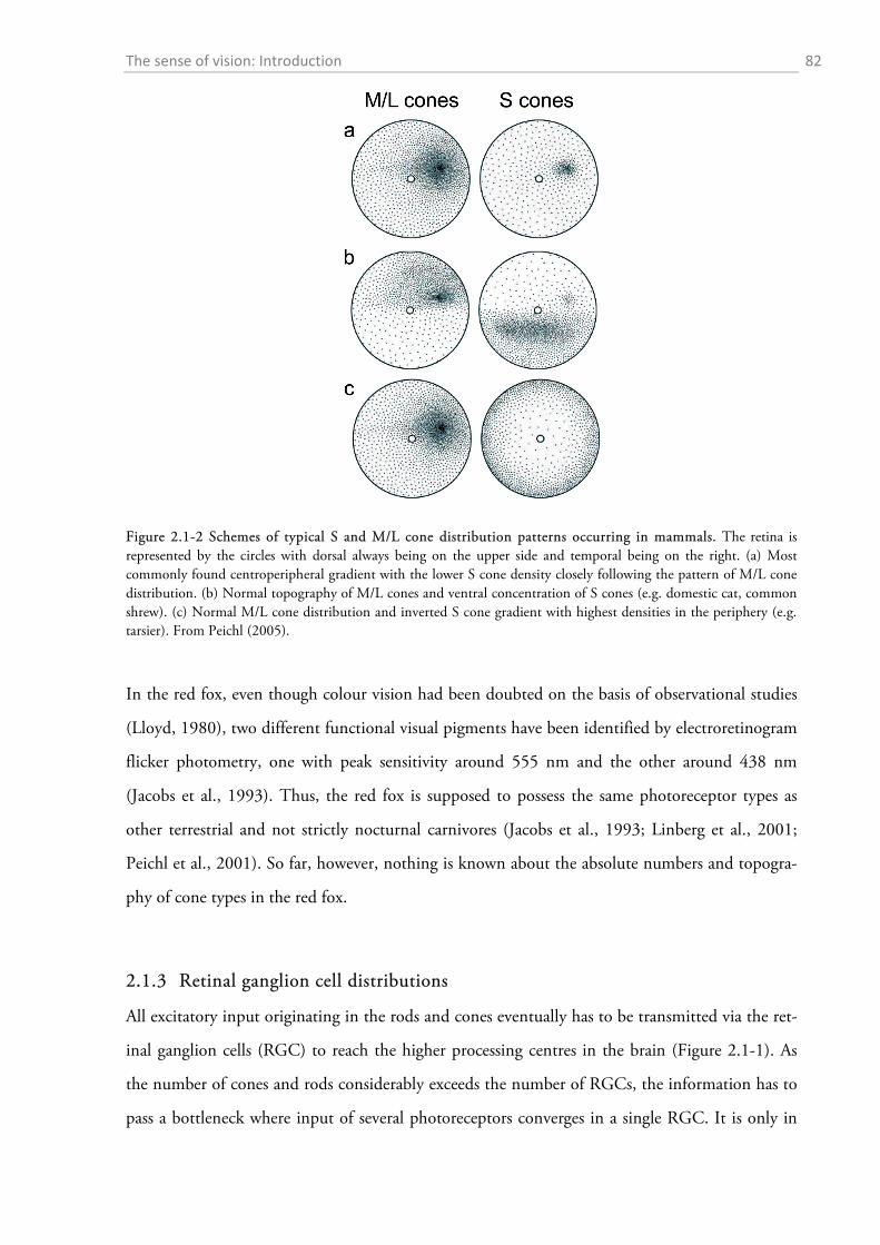
The sense of vision: Introduction 82
Figure 2.1-2 Schemes of typical S and M/L cone distribution patterns occurring in mammals. The retina is represented by the circles with dorsal always being on the upper side and temporal being on the right. (a) Most commonly found centroperipheral gradient with the lower S cone density closely following the pattern of M/L cone distribution. (b) Normal topography of M/L cones and ventral concentration of S cones (e.g. domestic cat, common shrew). (c) Normal M/L cone distribution and inverted S cone gradient with highest densities in the periphery (e.g. tarsier). From Peichl (2005).
In the red fox, even though colour vision had been doubted on the basis of observational studies
(Lloyd, 1980), two different functional visual pigments have been identified by electroretinogram
flicker photometry, one with peak sensitivity around 555 nm and the other around 438 nm
(Jacobs et al., 1993). Thus, the red fox is supposed to possess the same photoreceptor types as
other terrestrial and not strictly nocturnal carnivores (Jacobs et al., 1993; Linberg et al., 2001;
Peichl et al., 2001). So far, however, nothing is known about the absolute numbers and topogra-
phy of cone types in the red fox.
2.1.3 Retinal ganglion cell distributions
All excitatory input originating in the rods and cones eventually has to be transmitted via the ret-
inal ganglion cells (RGC) to reach the higher processing centres in the brain (Figure 2.1-1). As
the number of cones and rods considerably exceeds the number of RGCs, the information has to
pass a bottleneck where input of several photoreceptors converges in a single RGC. It is only in
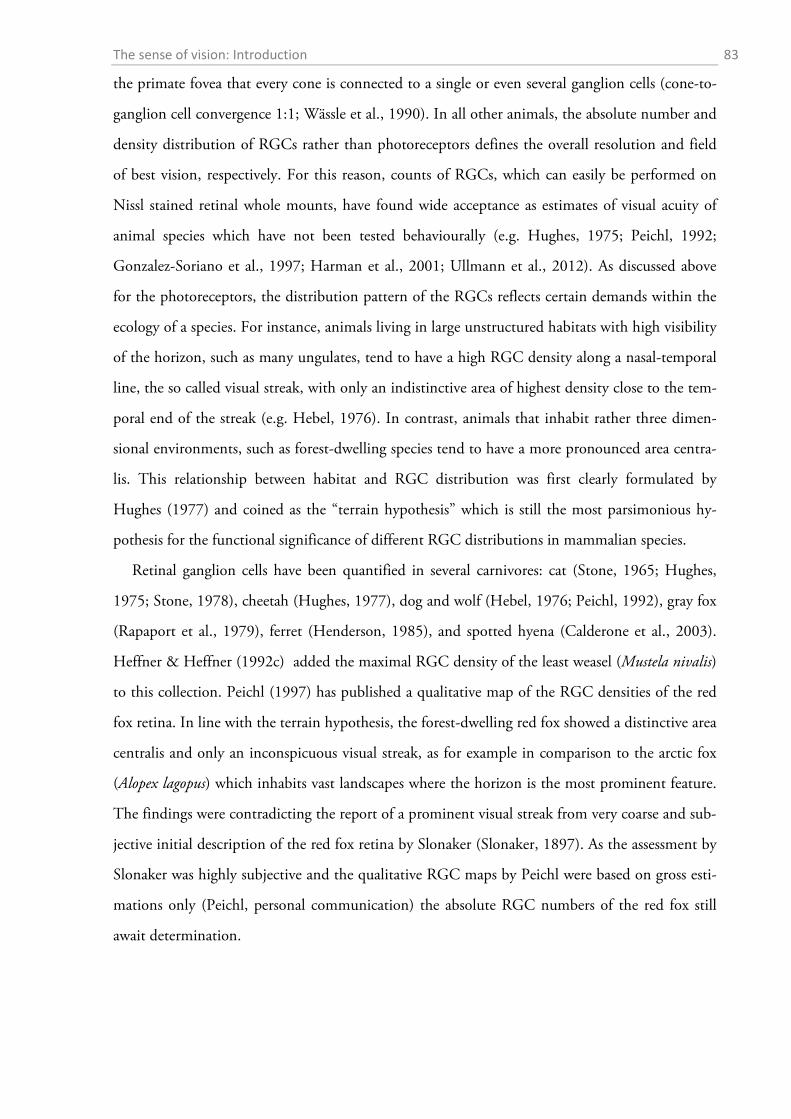
The sense of vision: Introduction 83
the primate fovea that every cone is connected to a single or even several ganglion cells (cone-to-
ganglion cell convergence 1:1; Wässle et al., 1990). In all other animals, the absolute number and
density distribution of RGCs rather than photoreceptors defines the overall resolution and field
of best vision, respectively. For this reason, counts of RGCs, which can easily be performed on
Nissl stained retinal whole mounts, have found wide acceptance as estimates of visual acuity of
animal species which have not been tested behaviourally (e.g. Hughes, 1975; Peichl, 1992;
Gonzalez‐Soriano et al., 1997; Harman et al., 2001; Ullmann et al., 2012). As discussed above
for the photoreceptors, the distribution pattern of the RGCs reflects certain demands within the
ecology of a species. For instance, animals living in large unstructured habitats with high visibility
of the horizon, such as many ungulates, tend to have a high RGC density along a nasal-temporal
line, the so called visual streak, with only an indistinctive area of highest density close to the tem-
poral end of the streak (e.g. Hebel, 1976). In contrast, animals that inhabit rather three dimen-
sional environments, such as forest-dwelling species tend to have a more pronounced area centra-
lis. This relationship between habitat and RGC distribution was first clearly formulated by
Hughes (1977) and coined as the “terrain hypothesis” which is still the most parsimonious hy-
pothesis for the functional significance of different RGC distributions in mammalian species.
Retinal ganglion cells have been quantified in several carnivores: cat (Stone, 1965; Hughes,
1975; Stone, 1978), cheetah (Hughes, 1977), dog and wolf (Hebel, 1976; Peichl, 1992), gray fox
(Rapaport et al., 1979), ferret (Henderson, 1985), and spotted hyena (Calderone et al., 2003).
Heffner & Heffner (1992c) added the maximal RGC density of the least weasel (Mustela nivalis)
to this collection. Peichl (1997) has published a qualitative map of the RGC densities of the red
fox retina. In line with the terrain hypothesis, the forest-dwelling red fox showed a distinctive area
centralis and only an inconspicuous visual streak, as for example in comparison to the arctic fox
(Alopex lagopus) which inhabits vast landscapes where the horizon is the most prominent feature.
The findings were contradicting the report of a prominent visual streak from very coarse and sub-
jective initial description of the red fox retina by Slonaker (Slonaker, 1897). As the assessment by
Slonaker was highly subjective and the qualitative RGC maps by Peichl were based on gross esti-
mations only (Peichl, personal communication) the absolute RGC numbers of the red fox still
await determination.
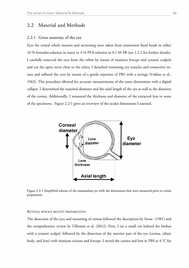
The sense of vision: Material & Methods 84
2.2 Material and Methods
2.2.1 Gross anatomy of the eye
Eyes for retinal whole mounts and sectioning were taken from immersion fixed heads in either
10 % formalin-solution in water or 4 % PFA-solution in 0.1 M PB (see 1.2.2 for further details).
I carefully removed the eyes from the orbits by means of titanium forceps and ceramic scalpels
and cut the optic nerve close to the sclera. I detached remaining eye muscles and connective tis-
sues and inflated the eyes by means of a gentle injection of PBS with a syringe (Vakkur et al.,
1963). This procedure allowed for accurate measurements of the outer dimensions with a digital
calliper. I determined the maximal diameter and the axial length of the eye as well as the diameter
of the cornea. Additionally, I measured the thickness and diameter of the extracted lens in some
of the specimens. Figure 2.2-1 gives an overview of the ocular dimensions I assessed.
Figure 2.2-1 Simplified scheme of the mammalian eye with the dimensions that were measured prior to retina preparation.
RETINAL WHOLE MOUNT PREPARATION
The dissection of the eyes and mounting of retinae followed the description by Stone (1981) and
the comprehensive review by Ullmann et al. (2012). First, I set a small cut behind the limbus
with a ceramic scalpel, followed by the dissection of the anterior part of the eye (cornea, ciliary
body, and lens) with titanium scissors and forceps. I stored the cornea and lens in PBS at 4 °C for
The sense of vision: Material & Methods 85
later analysis. A small triangular incision allowed for later reorientation. To extract the retina
from the eyecup, I first carefully removed the vitreous body with help of titanium forceps and soft
brushes. Next, I freed the retina in small steps beginning at the margins by carefully inserting a
custom-sharpened and custom-bent raspatory (AF-Medical, Kreuzlingen, Switzerland) between
the retina and the pigment epithelium. When reaching the optic disc, I cut the optic nerve and
removed the retina from the eyecup. If pigment epithelium was still attached to the retina, I
bleached it for up to 45 minutes in a hydrogen peroxide bleaching solution (recipe given in the
appendix). After bleaching, I thoroughly washed the retina in 0.1 M PB.
OPSIN IMMUNOHISTOCHEMISTRY
The preparation of the retinae followed the same protocol as for the RGC staining, but for im-
munohistochemistry I processed the retinae free floating in a plastic petri dish (3.5 cm diameter)
before mounting them upside down onto an untreated microscope slide to promote visual access
to the photoreceptor layers after staining was completed. The visualization of the different cone
types was accomplished by immunohistochemistry of the S and L opsins according to the follow-
ing steps (all performed at ambient temperature):
wash the fixed and prepared retina in PB (0.1 M pH = 7.4; several times if the retina had
been bleached before)
incubate the retina in sucrose solutions of increasing concentrations (10 %, 20 %, 30 %
in PB) until the retina sinks to the bottom of the vial; at least 2 h in the 30 % solution
cracking: transfer the retina from the 30 %-sucrose solution onto a clean microscope slide
and quickly freeze it by holding it over a -80 °C metal cooling block; allow the retina to
thaw and repeated the procedure two more times
wash in 0.1 M PB
block with 1 ml 10 % normal goat serum (NGS) or normal donkey serum (NDS), 1 %
bovine serum albumin (BSA), 0.5 % Triton-X-100, 0.05 % sodium azide (NaN3) in PB
for 1 h
wash in 0.1 M PB
incubate with the first antibody diluted in 1 ml 3 % NGS or NDS, 1 % BSA, 0.5 % Tri-
ton-X-100, 0.05 % sodium azide in 0.1 M PB on a lab shaker for 3 days
wash in PB for at least 1 h
The sense of vision: Material & Methods 86
Diaminobenzidine (DAB)-staining:
incubate with the secondary antibodies diluted in 1 ml 3 % NGS or NDS, 1 % BSA,
0.5 % Triton-X, 0.05 % sodium azide in 0.1 M PB on a lab shaker overnight in darkness
wash for several hours in 0.1 M PB
incubate with xx-peroxidase anti peroxidase (xx-PAP with xx being the host species of the
primary antibodies) diluted in 1 ml 3 % NGS or NDS, 1 % BSA, 0.5 % Triton-X-100,
in 0.1 M PB (without sodium azide) on a lab shaker overnight
wash several times for several hours in 0.1 M PB (without sodium azide)
transfer retinae in 0.05 M Tris-buffer (pH = 7.6); change the buffer two times
15’ incubation in 1 ml 0.05 % DAB in 0.05 M Tris-buffer
5-8’ incubation in 1 ml 0.05 % DAB, 0.01 % H2O2 in 0.05 M Tris-buffer until staining
was sufficient
wash in 0.05 M Tris-buffer
wash 2-3 h in 0.1 M PB; change buffer several times
I mounted the retinae with Roti Histokit II® (Carl Roth) and analysed them at a bright field
microscope (Olympus BX40 or Zeiss Axio Observer Z1).
The following primary antibodies were used:
1. Rabbit antiserum JH 455 raised against the last 38 amino acids of the human S (blue)
cone opsin (kindly provided by J. Nathans; characterised by Wang et al., 1992).
2. Rabbit antiserum JH 492 raised against the last 38 amino acids of the human L (red)
cone opsin (kindly provided by J. Nathans; characterised by Wang et al., 1992).
I determined the outer dimensions of 37 eyes from 19 different foxes. As in the previous chap-
ter, I assorted the animals to three age classes (juvenile, subadult, adult) according to their CBL
values (interpolated from the findings by Hartová-Nentvichová et al., 2010). The sample distri-
bution was skewed towards younger animals with ten juveniles and seven subadults, while the
eyes of only three adult specimens could be studied.
The sense of vision: Material & Methods 87
RETINAL GANGLION CELL STAINING
For staining of RGCs, I mounted the retinae with their anterior side (RGC layer) up on a gelati-
nized (5 %) microscope slide (76 mm x 52 mm, Carl Roth). Three to four radial cuts served to
flatten the retina. I carefully removed remaining vitreous humour with a soft brush.
To attach the retina to the gelatinized slide, I employed the sandwich method (Figure 2.2-2,
Peichl, personal communication). I covered the retina with two sheets of lens cleaning paper
(Olympus) with a single layer of filter paper (Whatman, Kent, UK) in between. An uncoated mi-
croscope slide and a 54 g brass weight covered the top, and the whole sandwich was placed over-
night in a 9:1 solution of 96 % ethanol and 37 % formalin. I soaked all paper sheets and cover
slides with the ethanol-formalin solution before usage.
I used a Nissl stain for RGC visualization according to the following protocol:
45’ incubation of the mounted retina in a solution of 95 % ethanol + 5 % acetic acid
rinse in aq. dest.
staining with 0.1 % cresyl violet until RGC layer (only) is clearly recognizable depend-
ing on the freshness of the dye solution incubate between 30” and 5’
control staining success under the microscope and stop in time by rinsing in aq. dest.
30” 70 % ethanol
5-7’ 100 % ethanol
20’ xylen
I mounted the retinae with Roti Histokit II® (Carl Roth) and analysed them at a bright field mi-
croscope (BX40, Olympus or Axio Observer Z1, Carl Zeiss AG, Jena, Germany).
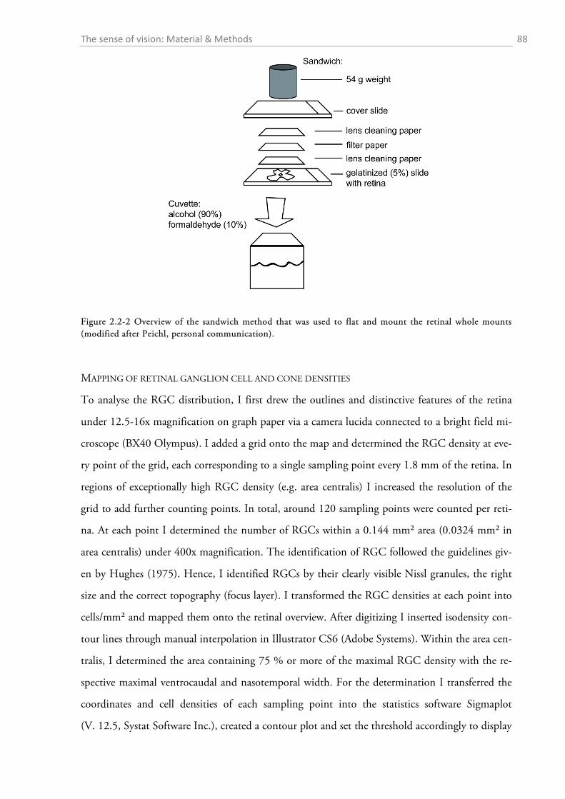
The sense of vision: Material & Methods 88
Figure 2.2-2 Overview of the sandwich method that was used to flat and mount the retinal whole mounts (modified after Peichl, personal communication).
MAPPING OF RETINAL GANGLION CELL AND CONE DENSITIES
To analyse the RGC distribution, I first drew the outlines and distinctive features of the retina
under 12.5-16x magnification on graph paper via a camera lucida connected to a bright field mi-
croscope (BX40 Olympus). I added a grid onto the map and determined the RGC density at eve-
ry point of the grid, each corresponding to a single sampling point every 1.8 mm of the retina. In
regions of exceptionally high RGC density (e.g. area centralis) I increased the resolution of the
grid to add further counting points. In total, around 120 sampling points were counted per reti-
na. At each point I determined the number of RGCs within a 0.144 mm² area (0.0324 mm² in
area centralis) under 400x magnification. The identification of RGC followed the guidelines giv-
en by Hughes (1975). Hence, I identified RGCs by their clearly visible Nissl granules, the right
size and the correct topography (focus layer). I transformed the RGC densities at each point into
cells/mm² and mapped them onto the retinal overview. After digitizing I inserted isodensity con-
tour lines through manual interpolation in Illustrator CS6 (Adobe Systems). Within the area cen-
tralis, I determined the area containing 75 % or more of the maximal RGC density with the re-
spective maximal ventrocaudal and nasotemporal width. For the determination I transferred the
coordinates and cell densities of each sampling point into the statistics software Sigmaplot
(V. 12.5, Systat Software Inc.), created a contour plot and set the threshold accordingly to display
The sense of vision: Material & Methods 89
the boundaries of the 75 % area. ImageJ (1.48v, NIH) then allowed the measurement of the area
and linear dimensions. As the retina had been fixed to the gelatinized slide already at the begin-
ning of the staining procedure, I assumed, referring to other reports (Wässle et al., 1975, 1981),
shrinkage artefacts to be neglectable and did not correct for it.
The procedure of mapping the distribution of photopigments (S and M/L cones) was different
from the RGC procedure. I scanned the whole immunostained retina at high-magnification with
help of an inverted microscope with an automated stage (Zeiss Axio Observer Z1) at 200x magni-
fication. To ensure sharp imaging of the desired plane at all positions, a Z-stack was created of
5-8 planes with 6-8 µm spacing at each sampling point. Additionally, as the surface of the speci-
mens was not fully even, the focus had to be adjusted by setting 50-60 focus points between
which the microscope automatically used interpolated values. The resulting image of the retina
consisted of approximately 2,000 single images (each at 200x magnification) which were auto-
matically stitched together with the image processing software ZEN (V. 2012., Zeiss) to yield a
coherent and non-overlapping image of the retinal specimen. To map the density of the cones, I
overlaid a grid (spacing 1.8 mm) within the ZEN software and counted all immunopositive cells
at each of the approximately 120 grid positions within a 0.04 mm² area at 200x magnification. I
interpolated the respective cone densities per mm² and mapped them onto the retinal overview.
Finally, to visualize the distribution, I transferred the coordinates and cell densities of each sam-
pling point into the statistics software Sigmaplot (V. 12.5, Systat Software Inc.) to create contour
plots which I subsequently fitted into outlines of the retina. Here, to achieve full mapping cover-
age of the whole retina, I added a few additional points with slightly lower values relative to those
sampled along the retinal periphery and placed these beyond the retinal outlines. I did not correct
for tissue shrinkage (cf. Calderone et al., 2003; Schiviz et al., 2008).
2.2.2 Estimates of visual acuity
The external measurements of the eye and retinal cell densities were used to estimate the visual
acuity of the red fox. As no schematic eye exists for the red fox and the establishment of such a
model was beyond the scope of this thesis (cf. Vakkur & Bishop, 1963; Hughes, 1977, 1979;
Coile & O'Keefe, 1988 for the technical and computational demands of developing such a
model), I determined the retinal magnification factor (RMF) by two different approximate meth-
ods and used the mean for all further calculations. First, as comparative studies have shown that
The sense of vision: Material & Methods 90
the RMF is linearly related to the axial length of the eye (Hughes, 1977), I calculated the respec-
tive RMF for the red fox by placing the mean axial length (AL) into the equation of the regression
line:
RMF �mmdeg
� = 0.011 ( 1deg
) × AL(mm) (Hughes, 1977).
Additionally, I determined the RMF with help of the estimated posterior nodal distance
(PND) by multiplying the axial length of the eye by 0.54, the axial length/PND ratio (Pettigrew
et al., 1988). I chose this specific ratio for the red fox because the published ratios of strictly noc-
turnal animals ranged from 0.51-0.54, while the respective ratios of crepuscular animals were be-
tween 0.54 and 0.6 (Pettigrew et al., 1988). Within this spectrum I assorted the red fox to the
upper end of the nocturnal and the lower end of the crepuscular range, properly reflecting its
ecology. Using the PND, the RMF can be estimated as:
RMF (mm/deg) = 2π × PND (mm)360 (deg)
(Harman et al., 2001).
The number of cycles per mm can be calculated by dividing the number of ganglion cells per mm
(assuming a square sample array, the number can be estimated from the square root of the maxi-
mal density) in the region of highest density by two:
cycmm
= �maximal ganglion cell density2 cyc mm−1 .
Finally, I calculated the visual acuity in cycles per degree:
Visual acuity (cyc/deg) = RMF (𝑚𝑚𝑑𝑏𝑑
) × cycmm
.
The sense of vision: Material & Methods 91
2.2.3 Estimates of sound localization ability
The area of best vision, defined as the horizontal width (in degree) of the retinal area where the
density of RGCs reaches at least 75 %, is strongly inversely correlated to the sound localization
ability of mammals (Heffner & Heffner, 1992c). To estimate this value for the red fox, I deter-
mined the horizontal width of the 75 % RGC density area (measurement described above) and
the species-specific RMF as described above. The resulting value of the field of best vision in de-
grees served then to estimate the sound localization threshold of the red fox (in degrees) by means
of the regression that I obtained by plotting the field of vision and sound localization threshold
data published in Heffner & Heffner (1992c) on a double-logarithmic scale:
sound localization threshold (deg) = 1.8422 × (field of best vision (deg)0.5588).
2.2.4 Statistics and graphics
I employed Sigmaplot (V. 12.5, Systat Software Inc.) to plot all graphs and perform descriptive
statistics and statistical interference. Variance equality and normal distribution were always tested
with Bartlett’s test and test procedure by Shapiro-Wilk, respectively. In case of normal distribu-
tions, I performed t-tests or analyses of variance (ANOVA) depending on the structure of the da-
ta (procedure always given in the results section). Nonparametric tests comprised Mann-Whitney
U-test and ANOVA on ranks. Advanced statistical tests and analyses are indicated with the re-
spective results in the results section. For tables, standard calculations, and data transformation I
used Excel 2010 (Microsoft Corp.). I prepared graphical illustrations in Photoshop and Illustrator
CS6 (Adobe Systems) and performed graphical metrics and cell counts in ImageJ (V. 1.48v,
NIH).
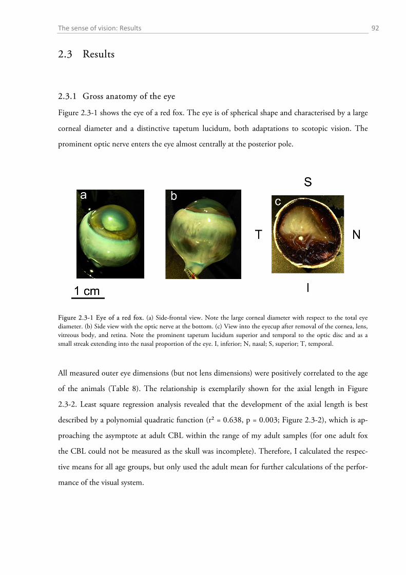
The sense of vision: Results 92
2.3 Results
2.3.1 Gross anatomy of the eye
Figure 2.3-1 shows the eye of a red fox. The eye is of spherical shape and characterised by a large
corneal diameter and a distinctive tapetum lucidum, both adaptations to scotopic vision. The
prominent optic nerve enters the eye almost centrally at the posterior pole.
Figure 2.3-1 Eye of a red fox. (a) Side-frontal view. Note the large corneal diameter with respect to the total eye diameter. (b) Side view with the optic nerve at the bottom. (c) View into the eyecup after removal of the cornea, lens, vitreous body, and retina. Note the prominent tapetum lucidum superior and temporal to the optic disc and as a small streak extending into the nasal proportion of the eye. I, inferior; N, nasal; S, superior; T, temporal.
All measured outer eye dimensions (but not lens dimensions) were positively correlated to the age
of the animals (Table 8). The relationship is exemplarily shown for the axial length in Figure
2.3-2. Least square regression analysis revealed that the development of the axial length is best
described by a polynomial quadratic function (r² = 0.638, p = 0.003; Figure 2.3-2), which is ap-
proaching the asymptote at adult CBL within the range of my adult samples (for one adult fox
the CBL could not be measured as the skull was incomplete). Therefore, I calculated the respec-
tive means for all age groups, but only used the adult mean for further calculations of the perfor-
mance of the visual system.
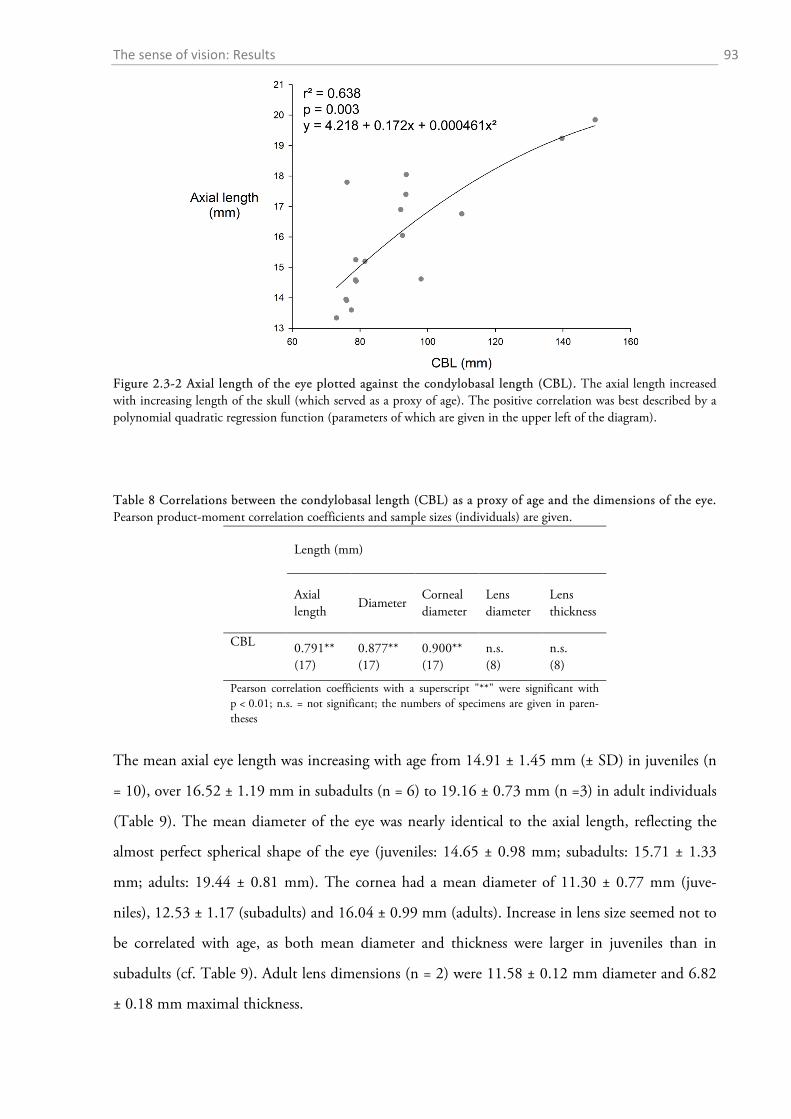
The sense of vision: Results 93
Figure 2.3-2 Axial length of the eye plotted against the condylobasal length (CBL). The axial length increased with increasing length of the skull (which served as a proxy of age). The positive correlation was best described by a polynomial quadratic regression function (parameters of which are given in the upper left of the diagram).
Table 8 Correlations between the condylobasal length (CBL) as a proxy of age and the dimensions of the eye. Pearson product-moment correlation coefficients and sample sizes (individuals) are given.
Length (mm)
Axial length
Diameter Corneal diameter
Lens diameter
Lens thickness
CBL 0.791** (17)
0.877** (17)
0.900** (17)
n.s. (8)
n.s. (8)
Pearson correlation coefficients with a superscript "**" were significant with p < 0.01; n.s. = not significant; the numbers of specimens are given in paren-theses
The mean axial eye length was increasing with age from 14.91 ± 1.45 mm (± SD) in juveniles (n
= 10), over 16.52 ± 1.19 mm in subadults (n = 6) to 19.16 ± 0.73 mm (n =3) in adult individuals
(Table 9). The mean diameter of the eye was nearly identical to the axial length, reflecting the
almost perfect spherical shape of the eye (juveniles: 14.65 ± 0.98 mm; subadults: 15.71 ± 1.33
mm; adults: 19.44 ± 0.81 mm). The cornea had a mean diameter of 11.30 ± 0.77 mm (juve-
niles), 12.53 ± 1.17 (subadults) and 16.04 ± 0.99 mm (adults). Increase in lens size seemed not to
be correlated with age, as both mean diameter and thickness were larger in juveniles than in
subadults (cf. Table 9). Adult lens dimensions (n = 2) were 11.58 ± 0.12 mm diameter and 6.82
± 0.18 mm maximal thickness.
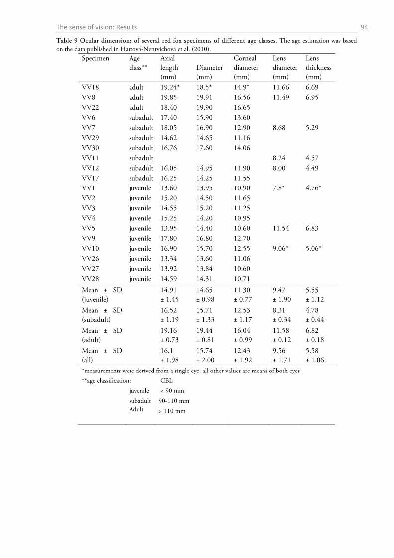
The sense of vision: Results 94
Table 9 Ocular dimensions of several red fox specimens of different age classes. The age estimation was based on the data published in Hartová-Nentvichová et al. (2010).
Specimen Age class**
Axial length (mm)
Diameter (mm)
Corneal diameter (mm)
Lens diameter (mm)
Lens thickness (mm)
VV18 adult 19.24* 18.5* 14.9* 11.66 6.69 VV8 adult 19.85 19.91 16.56 11.49 6.95 VV22 adult 18.40 19.90 16.65
VV6 subadult 17.40 15.90 13.60 VV7 subadult 18.05 16.90 12.90 8.68 5.29
VV29 subadult 14.62 14.65 11.16 VV30 subadult 16.76 17.60 14.06 VV11 subadult
8.24 4.57
VV12 subadult 16.05 14.95 11.90 8.00 4.49 VV17 subadult 16.25 14.25 11.55
VV1 juvenile 13.60 13.95 10.90 7.8* 4.76* VV2 juvenile 15.20 14.50 11.65
VV3 juvenile 14.55 15.20 11.25 VV4 juvenile 15.25 14.20 10.95 VV5 juvenile 13.95 14.40 10.60 11.54 6.83
VV9 juvenile 17.80 16.80 12.70 VV10 juvenile 16.90 15.70 12.55 9.06* 5.06*
VV26 juvenile 13.34 13.60 11.06 VV27 juvenile 13.92 13.84 10.60 VV28 juvenile 14.59 14.31 10.71
Mean ± SD (juvenile)
14.91 ± 1.45
14.65 ± 0.98
11.30 ± 0.77
9.47 ± 1.90
5.55 ± 1.12
Mean ± SD (subadult)
16.52 ± 1.19
15.71 ± 1.33
12.53 ± 1.17
8.31 ± 0.34
4.78 ± 0.44
Mean ± SD (adult)
19.16 ± 0.73
19.44 ± 0.81
16.04 ± 0.99
11.58 ± 0.12
6.82 ± 0.18
Mean ± SD (all)
16.1 ± 1.98
15.74 ± 2.00
12.43 ± 1.92
9.56 ± 1.71
5.58 ± 1.06
*measurements were derived from a single eye, all other values are means of both eyes **age classification: CBL
juvenile < 90 mm subadult 90-110 mm
Adult > 110 mm
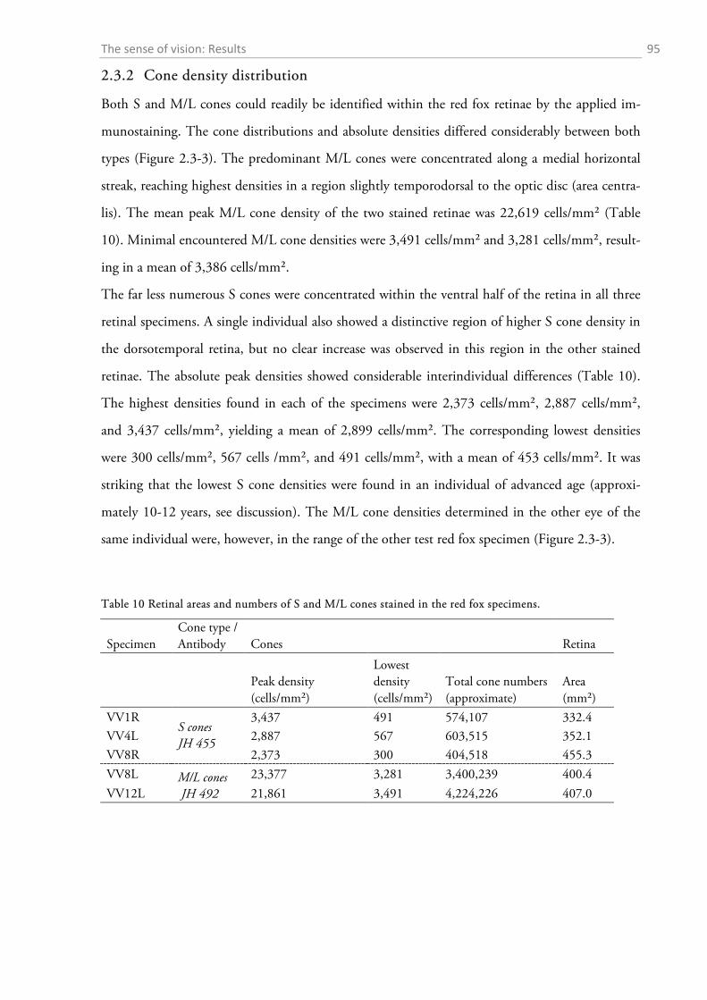
The sense of vision: Results 95
2.3.2 Cone density distribution
Both S and M/L cones could readily be identified within the red fox retinae by the applied im-
munostaining. The cone distributions and absolute densities differed considerably between both
types (Figure 2.3-3). The predominant M/L cones were concentrated along a medial horizontal
streak, reaching highest densities in a region slightly temporodorsal to the optic disc (area centra-
lis). The mean peak M/L cone density of the two stained retinae was 22,619 cells/mm² (Table
10). Minimal encountered M/L cone densities were 3,491 cells/mm² and 3,281 cells/mm², result-
ing in a mean of 3,386 cells/mm².
The far less numerous S cones were concentrated within the ventral half of the retina in all three
retinal specimens. A single individual also showed a distinctive region of higher S cone density in
the dorsotemporal retina, but no clear increase was observed in this region in the other stained
retinae. The absolute peak densities showed considerable interindividual differences (Table 10).
The highest densities found in each of the specimens were 2,373 cells/mm², 2,887 cells/mm²,
and 3,437 cells/mm², yielding a mean of 2,899 cells/mm². The corresponding lowest densities
were 300 cells/mm², 567 cells /mm², and 491 cells/mm², with a mean of 453 cells/mm². It was
striking that the lowest S cone densities were found in an individual of advanced age (approxi-
mately 10-12 years, see discussion). The M/L cone densities determined in the other eye of the
same individual were, however, in the range of the other test red fox specimen (Figure 2.3-3).
Table 10 Retinal areas and numbers of S and M/L cones stained in the red fox specimens.
Specimen Cone type / Antibody Cones Retina
Peak density (cells/mm²)
Lowest density (cells/mm²)
Total cone numbers (approximate)
Area (mm²)
VV1R S cones JH 455
3,437 491 574,107 332.4 VV4L 2,887 567 603,515 352.1 VV8R 2,373 300 404,518 455.3 VV8L M/L cones
JH 492 23,377 3,281 3,400,239 400.4
VV12L 21,861 3,491 4,224,226 407.0
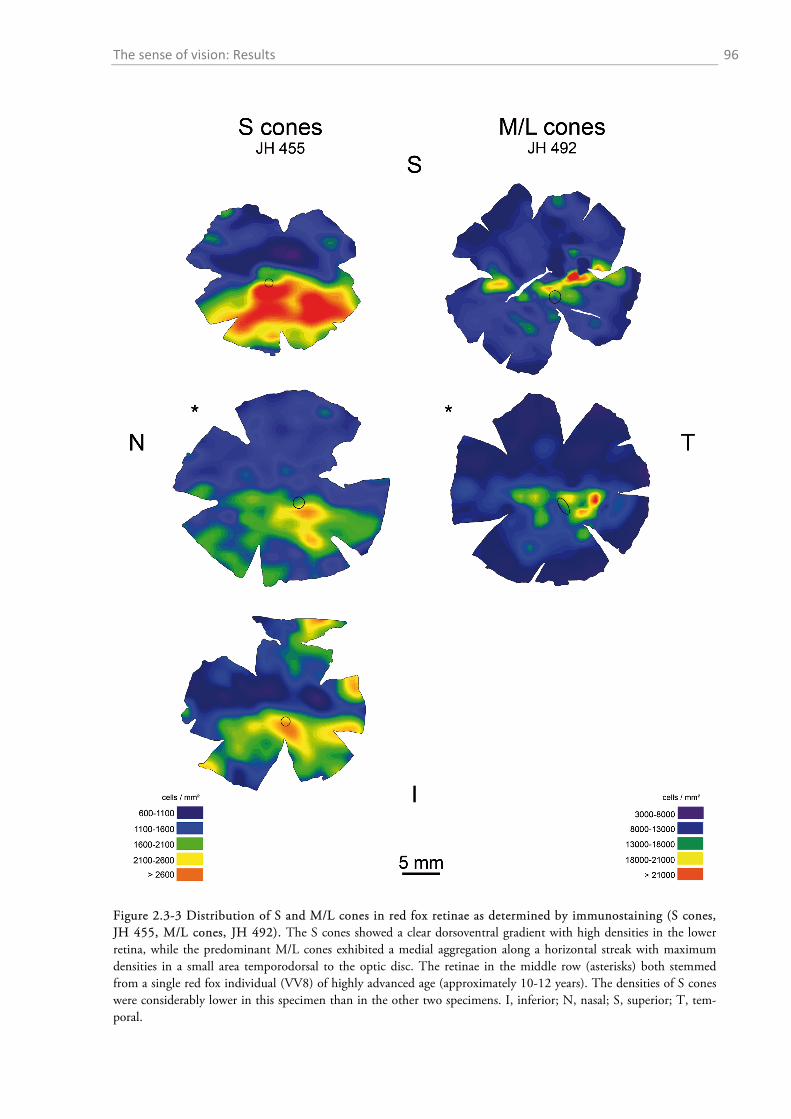
The sense of vision: Results 96
Figure 2.3-3 Distribution of S and M/L cones in red fox retinae as determined by immunostaining (S cones, JH 455, M/L cones, JH 492). The S cones showed a clear dorsoventral gradient with high densities in the lower retina, while the predominant M/L cones exhibited a medial aggregation along a horizontal streak with maximum densities in a small area temporodorsal to the optic disc. The retinae in the middle row (asterisks) both stemmed from a single red fox individual (VV8) of highly advanced age (approximately 10-12 years). The densities of S cones were considerably lower in this specimen than in the other two specimens. I, inferior; N, nasal; S, superior; T, tem-poral.
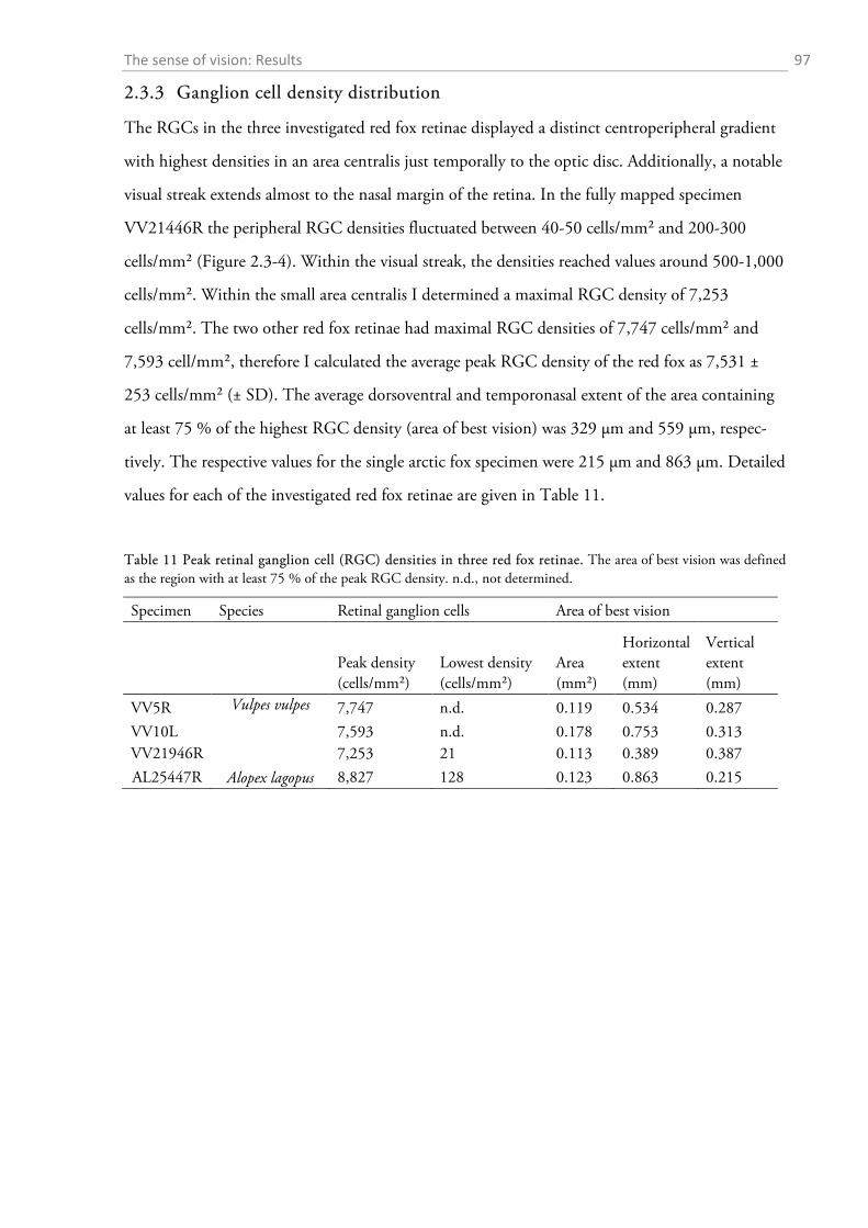
The sense of vision: Results 97
2.3.3 Ganglion cell density distribution
The RGCs in the three investigated red fox retinae displayed a distinct centroperipheral gradient
with highest densities in an area centralis just temporally to the optic disc. Additionally, a notable
visual streak extends almost to the nasal margin of the retina. In the fully mapped specimen
VV21446R the peripheral RGC densities fluctuated between 40-50 cells/mm² and 200-300
cells/mm² (Figure 2.3-4). Within the visual streak, the densities reached values around 500-1,000
cells/mm². Within the small area centralis I determined a maximal RGC density of 7,253
cells/mm². The two other red fox retinae had maximal RGC densities of 7,747 cells/mm² and
7,593 cell/mm², therefore I calculated the average peak RGC density of the red fox as 7,531 ±
253 cells/mm² (± SD). The average dorsoventral and temporonasal extent of the area containing
at least 75 % of the highest RGC density (area of best vision) was 329 µm and 559 µm, respec-
tively. The respective values for the single arctic fox specimen were 215 µm and 863 µm. Detailed
values for each of the investigated red fox retinae are given in Table 11.
Table 11 Peak retinal ganglion cell (RGC) densities in three red fox retinae. The area of best vision was defined as the region with at least 75 % of the peak RGC density. n.d., not determined.
Specimen Species Retinal ganglion cells Area of best vision
Peak density (cells/mm²)
Lowest density (cells/mm²)
Area (mm²)
Horizontal extent (mm)
Vertical extent (mm)
VV5R Vulpes vulpes 7,747 n.d. 0.119 0.534 0.287 VV10L 7,593 n.d. 0.178 0.753 0.313 VV21946R 7,253 21 0.113 0.389 0.387 AL25447R Alopex lagopus 8,827 128 0.123 0.863 0.215
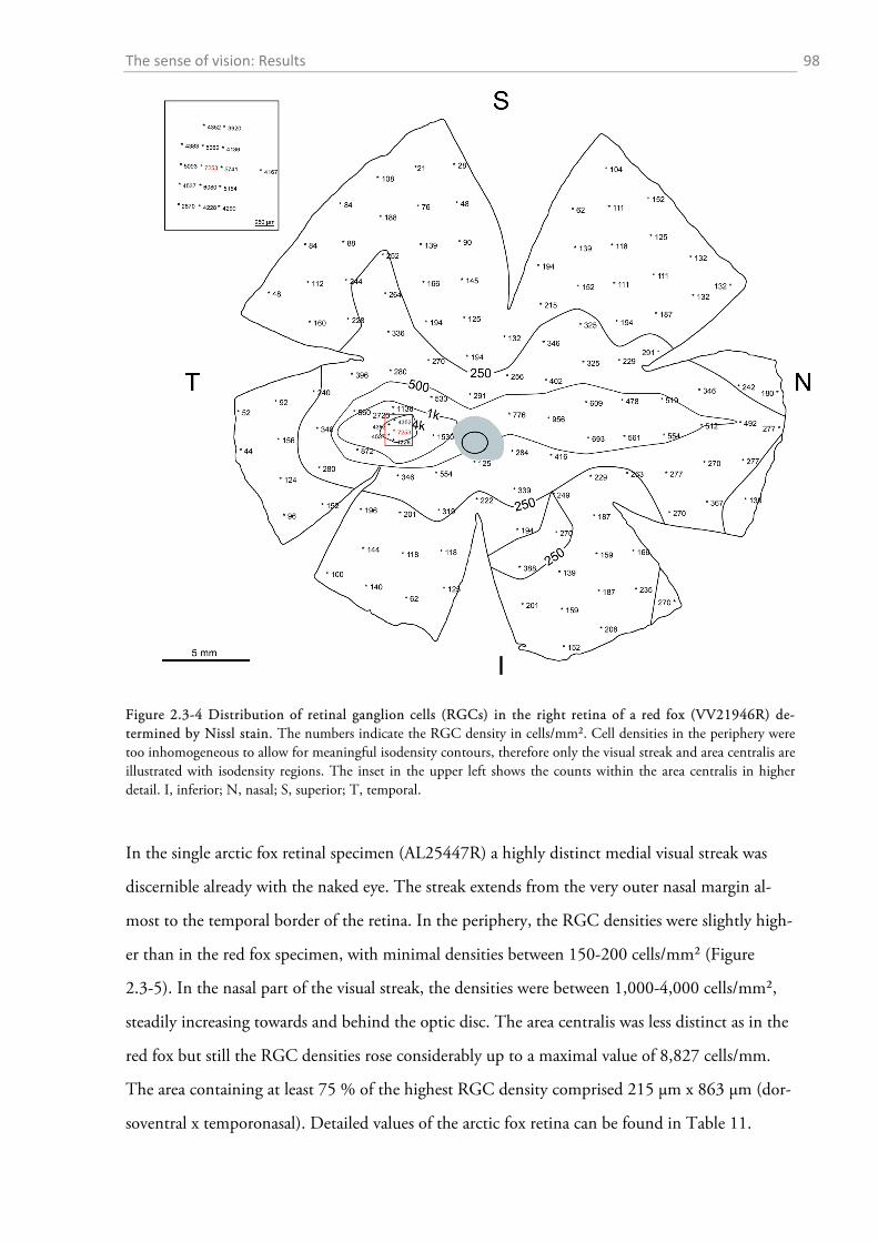
The sense of vision: Results 98
Figure 2.3-4 Distribution of retinal ganglion cells (RGCs) in the right retina of a red fox (VV21946R) de-termined by Nissl stain. The numbers indicate the RGC density in cells/mm². Cell densities in the periphery were too inhomogeneous to allow for meaningful isodensity contours, therefore only the visual streak and area centralis are illustrated with isodensity regions. The inset in the upper left shows the counts within the area centralis in higher detail. I, inferior; N, nasal; S, superior; T, temporal.
In the single arctic fox retinal specimen (AL25447R) a highly distinct medial visual streak was
discernible already with the naked eye. The streak extends from the very outer nasal margin al-
most to the temporal border of the retina. In the periphery, the RGC densities were slightly high-
er than in the red fox specimen, with minimal densities between 150-200 cells/mm² (Figure
2.3-5). In the nasal part of the visual streak, the densities were between 1,000-4,000 cells/mm²,
steadily increasing towards and behind the optic disc. The area centralis was less distinct as in the
red fox but still the RGC densities rose considerably up to a maximal value of 8,827 cells/mm.
The area containing at least 75 % of the highest RGC density comprised 215 µm x 863 µm (dor-
soventral x temporonasal). Detailed values of the arctic fox retina can be found in Table 11.
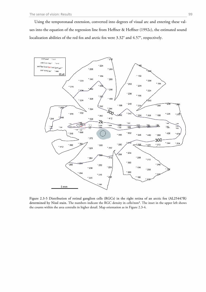
The sense of vision: Results 99
Using the temporonasal extension, converted into degrees of visual arc and entering these val-
ues into the equation of the regression line from Heffner & Heffner (1992c), the estimated sound
localization abilities of the red fox and arctic fox were 3.32° and 4.57°, respectively.
Figure 2.3-5 Distribution of retinal ganglion cells (RGCs) in the right retina of an arctic fox (AL25447R) determined by Nissl stain. The numbers indicate the RGC density in cells/mm². The inset in the upper left shows the counts within the area centralis in higher detail. Map orientation as in Figure 2.3-4.
The sense of vision: Results 100
2.3.4 Visual acuity of the red fox
Using the adult mean axial length of 19.16 mm, yielded red fox RMF estimations of
0.21 mm/deg (Hughes, 1977) and 0.18 mm/deg (Pettigrew et al., 1988; Harman et al., 2001),
resulting in a mean of 0.195 mm/deg. With the averaged peak RGC density of the three investi-
gated red fox specimens of 7,531 cells/mm² the cycle number calculated as 43.39 cyc/mm, which
totalled in a visual acuity of 8.46 cyc/deg of viewing angle.
Performing the same calculations with the data for the single arctic fox eye (axial length:
17 mm) yielded an estimated RMF of 0.17 mm/deg (I chose the same axial length/PND ratio of
0.54, based on the predominant nocturnal activity pattern reported by Audet et al., 2002). With
a maximal RGC density of 8,827 cells/mm², the visual acuity of the arctic fox specimen thus was
estimated as 7.99 cyc/deg.
The sense of vision: Discussion 101
2.4 Discussion
2.4.1 General ocular dimensions and ontogenetic development
The eyes of the red fox are typical for a nocturnal carnivore, with a relatively large cornea and a
well-developed tapetum lucidum. Details on the optical apparatus of lens and pupil of the red fox
have been described elsewhere (Malmström & Kröger, 2006), so I will not elaborate on this here.
Compared to the cat, the eyes of the red fox are a bit smaller but of the same globular shape (axial
length to diameter ratio 1:1.02; in the cat 1:1.03 (Vakkur et al., 1963). Because eye size strongly
correlates with body size, the smaller eyes in the larger red fox underline the supposition that it
relies more on other senses, such as olfaction and hearing than the cat (Österholm, 1964;
Nummela et al., 2013). The smaller eye size of the arctic fox compared to the red fox, on the oth-
er hand, is most probably not related to ecological factors but a simple consequence of its smaller
body size (Larivière & Pasitschniak-Arts, 1996; Audet et al., 2002; Nummela et al., 2013).
Eye growth during ontogenetic development extends well into adulthood in the Mongolian
gerbil (Wilkinson, 1986), the cat (Olson & Freeman, 1980), and even in humans (Scammon &
Armstrong, 1925), and might be a general mammalian trait during development. Changes in the
weight of the lens have already been reported for the red fox and were suggested to serve as a
means of age determination (Cavallini & Santini, 1995; in accordance with the results presented
here, lens weight alone was not an accurate predictor). Therefore, the strong correlation between
eye size and CBL in my fox sample is not astonishing. As to the use of CBL as a proxy of age,
Figure 2.3-2 shows that the growth rate of red foxes’ eyes decreases considerably for foxes with
CBLs ranging between 110 and 140 mm, and together with the good correspondence with axial
eye lengths of adult red foxes given by other authors (e.g. 20.55 mm; Nummela et al., 2013;
19 mm, 20 mm; Peichl, personal communication), the use of data from foxes with CBL > 110
mm as an estimate of the visual acuity of adult red foxes can be justified.
The significant developmental changes in the axial length of the eyes strongly alter the retinal
magnification factor (RMF) and consequently should affect visual acuity. In kittens, adult visual
acuity is reached earlier than adult eye size (Mitchell et al., 1976), so that mechanisms compen-
sating for the changes in ocular morphology can be assumed. It has been reported that distribu-
tion and absolute RGC density undergo significant changes during postnatal development in the
rat (McCall et al., 1987) and the cat (Alfred & Stone, 1982; Wong & Hughes, 1987). Therefore,
The sense of vision: Discussion 102
it would be interesting to study whether the density of RGCs in red foxes follows this develop-
mental pattern and maybe compensates for the reduced RMF, thus keeping the visual acuity
more or less constant. In doing so, also the development of the corneal curvature would have to
be taken into account. However, this would require studying the RGC distribution in a suffi-
ciently large number of foxes of different age, which was not feasible within the scope of the cur-
rent study.
2.4.2 Opsin distribution
The topography of S and M/L cones within the red fox retina follows a similar pattern as in other
carnivores, such as the cat (Linberg et al., 2001), the spotted hyena (Calderone et al., 2003), the
lion (Ahnelt et al., 2006), and the dog (beagle; Mowat et al., 2008). In all these species the high-
est densities of S cones are found in the ventral half-retina, while M/L cones predominate more
dorsally and often along a horizontal streak and within the area centralis. Ahnelt et al. (2006) ar-
gued that this pattern seems to be typical for animals living in open habitats such as the African
savannah, while forest-dwelling animals such as lynx, tiger, or deer exhibit a more concentric ar-
rangement of S cones. Both the (wild) cat and the red fox contradict this hypothesis. With respect
to the three most common stereotypical S cone distributions among mammals (Figure 2.1-2),
they possess a pattern which is in general quite common among small mammals as seen in nu-
merous rodents (Szél et al., 1994; Calderone & Jacobs, 2003; Haverkamp et al., 2005; Williams
et al., 2005), the rabbit (Juliusson et al., 1994), as well as all insectivores studied so far (Peichl et
al., 2000; Glösmann et al., 2008). The most common and intuitive explanation for this peculiar
cone arrangement is based on the close match between the dominant wavelengths reaching each
hemisphere of the visual field from the environment with the peak absorption of the S and M/L
cones. According to this hypothesis, in small rodents the upper hemisphere will mainly be excited
by longer wavelengths reflected from grass, earth, and leaf litter, while the lower hemisphere will
receive a considerably higher amount of short wavelengths from the sky (Veilleux & Kirk, 2014).
The higher sensitivity for short wavelengths in this part of the retina would hence be an adapta-
tion to enhance the contrast between the sky and objects within the sky, such as aerial predators
(coined as the "skylight hypothesis"; Szél et al., 1996). This simple “colour-match” explanation
has lately been questioned by Baden et al. (2013), demonstrating that the achromatic response
properties of the S cones rather than the spectral sensitivity makes them more suitable for detect-
The sense of vision: Discussion 103
ing dark objects in front of a bright background, while M/L cones respond equally to light and
dark stimuli (with opposite gain). Regardless of the underlying physiological mechanism, the as-
sumption for the ultimate evolutionary mechanism supported by the findings is enhanced surviv-
al (or reduced mortality) by avoiding aerial predation. This explanation does not hold for the red
fox. Even though smaller fox species can under highly unnatural circumstances become the main
prey of aerial predators (Roemer et al., 2002), this factor is highly improbable to have driven the
evolution of photoreceptors in the red fox. The red fox is the largest fox species and in general
rather predator than prey of birds (e.g. Chavko et al., 2007), let alone the much larger hyena and
lion. Ahnelt et al. (2006) therefore proposed, that in these species the ventral S cone gradient is
related to the low head position during stalking and search for carrion. As the eye height might be
approximately similar for a fox and a stalking lion, this hypothesis seems plausible.
Another alternative explanation discussed for the variations in cone patterns confers to the ret-
inal areas that show variability are under relaxed evolutionary pressure and might represent an
ancestral state of opsin evolution. Developmental and phylogenetic constraints might have led to
interspecies differences in opsin patterns without actual functional relevance (Szél et al., 1996;
Temple, 2011). Supporting this theory, while contradicting the “visual environment” theory is
the fact that in some closely related mice species, apparently inhabiting the same visual environ-
ment, the S cone distributions differ considerably (Szél et al., 1994). It is quite certain that the
debate will be continued as cone distributions of more and more species as well as good data
about the visual environments relevant to individual species are revealed (an overview is given by
Temple, 2011).
In both the cat (Linberg et al., 2001; Ahnelt et al., 2006) and one of the fox specimens ana-
lysed here a second region of high S cone density is found along the temporodorsal rim of the
retina. Since the other two red fox retinae of my sample did not reveal such a secondary peak re-
gion and no factor such as age, sex, or general cone densities consistently varies and might explain
the difference, it remains open for speculation and future studies, whether it simply reflects inter-
individual differences and/or has functional implications.
The cone densities of the red fox fall within a range typical for canine and felid retinae (Table
12). In particular, the density fits well to those reported for the wolf and cat (Steinberg et al.,
1973; Linberg et al., 2001; Peichl et al., 2001), with the M/L cone minimal density being higher
than in the cat but lower than in the wolf, while maximal M/L densities are higher in the cat and
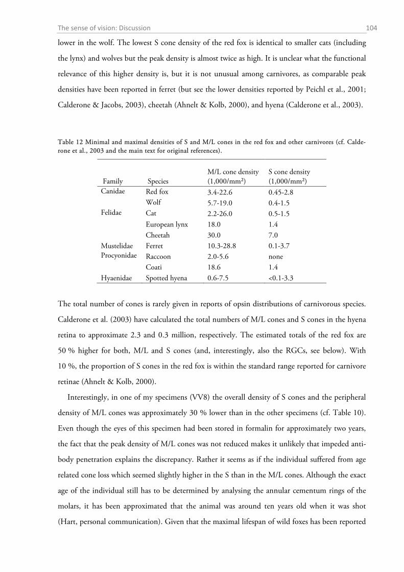
The sense of vision: Discussion 104
lower in the wolf. The lowest S cone density of the red fox is identical to smaller cats (including
the lynx) and wolves but the peak density is almost twice as high. It is unclear what the functional
relevance of this higher density is, but it is not unusual among carnivores, as comparable peak
densities have been reported in ferret (but see the lower densities reported by Peichl et al., 2001;
Calderone & Jacobs, 2003), cheetah (Ahnelt & Kolb, 2000), and hyena (Calderone et al., 2003).
Table 12 Minimal and maximal densities of S and M/L cones in the red fox and other carnivores (cf. Calde-rone et al., 2003 and the main text for original references).
Family Species M/L cone density (1,000/mm²)
S cone density (1,000/mm²)
Canidae Red fox 3.4-22.6 0.45-2.8 Wolf 5.7-19.0 0.4-1.5
Felidae Cat 2.2-26.0 0.5-1.5 European lynx 18.0 1.4 Cheetah 30.0 7.0
Mustelidae Ferret 10.3-28.8 0.1-3.7 Procyonidae Raccoon 2.0-5.6 none
Coati 18.6 1.4 Hyaenidae Spotted hyena 0.6-7.5 <0.1-3.3
The total number of cones is rarely given in reports of opsin distributions of carnivorous species.
Calderone et al. (2003) have calculated the total numbers of M/L cones and S cones in the hyena
retina to approximate 2.3 and 0.3 million, respectively. The estimated totals of the red fox are
50 % higher for both, M/L and S cones (and, interestingly, also the RGCs, see below). With
10 %, the proportion of S cones in the red fox is within the standard range reported for carnivore
retinae (Ahnelt & Kolb, 2000).
Interestingly, in one of my specimens (VV8) the overall density of S cones and the peripheral
density of M/L cones was approximately 30 % lower than in the other specimens (cf. Table 10).
Even though the eyes of this specimen had been stored in formalin for approximately two years,
the fact that the peak density of M/L cones was not reduced makes it unlikely that impeded anti-
body penetration explains the discrepancy. Rather it seems as if the individual suffered from age
related cone loss which seemed slightly higher in the S than in the M/L cones. Although the exact
age of the individual still has to be determined by analysing the annular cementum rings of the
molars, it has been approximated that the animal was around ten years old when it was shot
(Hart, personal communication). Given that the maximal lifespan of wild foxes has been reported
The sense of vision: Discussion 105
as 8.6 years (Larivière & Pasitschniak-Arts, 1996) it seems reasonable to assume that the individ-
ual had suffered from age related degenerations. Peripheral, but not central cone loss of up to
23 % has been reported in aged human individuals (Gao & Hollyfield, 1992; Curcio et al., 1993)
and S cones have been reported to be more vulnerable than the other cone types (Haegerstrom-
Portnoy et al., 1989). Therefore, I conclude that age related photoreceptor loss is witnessed in the
old red fox specimen.
2.4.3 Ganglion cell density and estimated sound localization acuity
In most mammals, the distribution of the ganglion cells closely follows the distribution of the
M/L cones (Ahnelt & Kolb, 2000). This holds true for the red fox, where both distributions are
characterised by a distinct density-increase around the area centralis and within a moderate hori-
zontal streak. The generally accepted hypothesis by Hughes (1977) states that the degree of the
expression of a visual streak is closely related to the environment the species is inhabiting. Species
in open habitats show generally prominent visual streaks as their predominant visual feature is the
horizon. The ganglion cell distribution of the arctic fox shows a very prominent streak and thus
perfectly fits to this theory. Also fittingly, the red fox RGC distribution is much more concentrat-
ed within the area centralis, reflecting the more silvicolous lifestyle of this species (Larivière &
Pasitschniak-Arts, 1996).
The peak RGC densities of the red fox and the arctic fox are approximately located in the
middle of the range reported for carnivores (cf. Table 13). They correspond well to the densities
reported for the cat (Hughes, 1975; Stone, 1978) while other canids tend to have considerably
higher peak densities, even though numbers in different dog breeds are highly variable (Peichl,
1992). RGC densities in many non-carnivores tend to be considerably lower.
The horizontal extent of the area containing at least 75 % of the peak RGC density allows
drawing inferences about the sound localization ability of a species (Heffner & Heffner, 1992c).
For the field of best vision determined in this study, the red fox would be predicted to have sound
localization acuity of 3-4°. At first glance this seems not to be in line with the reports of the max-
imal acuity of 1° given by Österholm (1964). However, having a closer look at the methods used
in the study by Österholm reveals several flaws that might explain the divergence. First, the pre-
sented sounds were much longer (2 s) than those used in contemporary studies of sound localiza-
tion acuity (100 ms). This is of importance as the former allows the fox to move the head and the
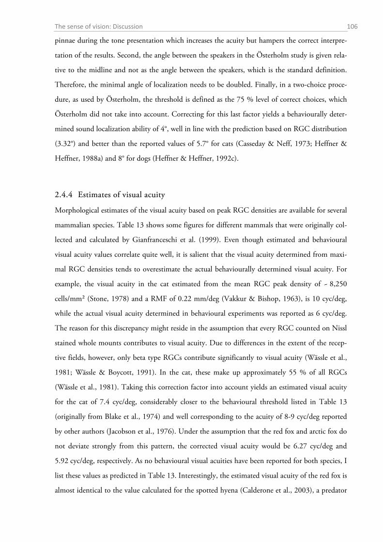
The sense of vision: Discussion 106
pinnae during the tone presentation which increases the acuity but hampers the correct interpre-
tation of the results. Second, the angle between the speakers in the Österholm study is given rela-
tive to the midline and not as the angle between the speakers, which is the standard definition.
Therefore, the minimal angle of localization needs to be doubled. Finally, in a two-choice proce-
dure, as used by Österholm, the threshold is defined as the 75 % level of correct choices, which
Österholm did not take into account. Correcting for this last factor yields a behaviourally deter-
mined sound localization ability of 4°, well in line with the prediction based on RGC distribution
(3.32°) and better than the reported values of 5.7° for cats (Casseday & Neff, 1973; Heffner &
Heffner, 1988a) and 8° for dogs (Heffner & Heffner, 1992c).
2.4.4 Estimates of visual acuity
Morphological estimates of the visual acuity based on peak RGC densities are available for several
mammalian species. Table 13 shows some figures for different mammals that were originally col-
lected and calculated by Gianfranceschi et al. (1999). Even though estimated and behavioural
visual acuity values correlate quite well, it is salient that the visual acuity determined from maxi-
mal RGC densities tends to overestimate the actual behaviourally determined visual acuity. For
example, the visual acuity in the cat estimated from the mean RGC peak density of ~ 8,250
cells/mm² (Stone, 1978) and a RMF of 0.22 mm/deg (Vakkur & Bishop, 1963), is 10 cyc/deg,
while the actual visual acuity determined in behavioural experiments was reported as 6 cyc/deg.
The reason for this discrepancy might reside in the assumption that every RGC counted on Nissl
stained whole mounts contributes to visual acuity. Due to differences in the extent of the recep-
tive fields, however, only beta type RGCs contribute significantly to visual acuity (Wässle et al.,
1981; Wässle & Boycott, 1991). In the cat, these make up approximately 55 % of all RGCs
(Wässle et al., 1981). Taking this correction factor into account yields an estimated visual acuity
for the cat of 7.4 cyc/deg, considerably closer to the behavioural threshold listed in Table 13
(originally from Blake et al., 1974) and well corresponding to the acuity of 8-9 cyc/deg reported
by other authors (Jacobson et al., 1976). Under the assumption that the red fox and arctic fox do
not deviate strongly from this pattern, the corrected visual acuity would be 6.27 cyc/deg and
5.92 cyc/deg, respectively. As no behavioural visual acuities have been reported for both species, I
list these values as predicted in Table 13. Interestingly, the estimated visual acuity of the red fox is
almost identical to the value calculated for the spotted hyena (Calderone et al., 2003), a predator
The sense of vision: Discussion 107
that presumably also relies more on other senses than vision (olfaction) to find its main food
items (carrion). Thus, even though a strong positive correlation between the axial length of
mammal eyes and their visual acuity has been revealed (Veilleux & Kirk, 2014) and the hyena eye
(axial length: 25.4 mm) is considerably larger than the red fox eye, it is a nice example of how
evolution has equipped the hyena eye with the optical properties just fitting the requirements of
its lifestyle. Having larger eyes than the red fox allowed the hyena to reduce the cone and RGC
densities, which reduces computational demands and saves energy. The opposite might have hap-
pened to the arctic fox, which had to increase the ganglion cell density (compared to the red fox)
in order to achieve comparable visual acuity with smaller eyes.
Table 13 Visual acuity in different mammalian species as estimated from their peak ganglion cell densities and ocular axial length, together with corresponding visual acuities determined behaviourally. I took the data shown in this table from Gianfranceschi et al. (1999), see the paper for references to the original studies. I corrected the data for the cat peak RGC densities reported by Gianfranceschi et al. (1999) as they did not correspond to those originally reported by Stone (1978). Also, the RMF of the rat and the estimates of the visual acuity of the dog and horse were corrected as they were wrongly calculated or cited by Gianfranceschi et al. (1999). Data on spotted hyena are taken from Calderone et al. (2003). I predicted the behavioural thresholds of both foxes by correcting the peak RGC density for the proportion of beta RGCs (see main text). n.d., not determined.
Species Peak RGC density (cells/mm²)
RMF (mm/deg)
Estimated visual acuity (cyc/deg)
Behavioural visual acuity (cyc/deg)
Cat Felis catus
8,250 0.22 10.0 6.0
Dog (beagle) Canis familiaris
12,200 0.18 9.9 6.3
Spotted hyena Crocuta crocuta
4,200 0.26 8.4 n.d.
Rabbit Oryctolagus cuniculus
2,500 0.17 4.3 3.4
Horse Equus ferus caballus
6,500 0.47 18.9 22.3
Rat Rattus norvegicus
2,000 0.059 1.3 1.0
Arctic fox Alopex lagopus
8,800 0.17 8.0 5.9 (predicted)
Red fox Vulpes vulpes
7,500 0.195 8.5 6.3 (predicted)
The magnetic sense: Introduction 108
3. MAGNETORECEPTION
3.1 Introduction
3.1.1 Magnetic orientation
The ability to perceive the geomagnetic field (GMF) and use it as a universal reference for orien-
tation has so far been demonstrated in more than 30 species of vertebrates with new ones being
reported regularly (reviewed in Wiltschko & Wiltschko, 1995; Wiltschko & Wiltschko, 2012a;
Begall et al., 2014). In the past, the majority of studies were done on birds. These studies have
given valuable insights into the functional properties of the magnetoreceptors (Wiltschko &
Wiltschko, 2010). In mammals, research on magnetoreception is far less advanced, but recently
the list of mammalian species expressing magnetosensitive behaviours is steadily growing
(reviewed in Begall et al., 2014).
The first mammals reported to have a magnetic sense were rodents. Early homing and orienta-
tion experiments with small epigeic rodents suggested that these mammals possess a magnetic
compass which they use for navigational purposes (Mather & Baker, 1981; August et al., 1989).
Later studies, however, challenged these findings with negative results and failed experimental
replications (Madden & Phillips, 1987; Sauvé, 1988) so that it was not until the early 1990s that
a robust behavioural assay was developed which provided solid and replicable evidence for magne-
toreception in mammals: the nest building assay (Burda et al., 1990). This paradigm, in which
the directions of nests built in a radial symmetrical arena are analysed, has been used ever since
with a variety of different species and has yielded first insights into the mechanisms of magneto-
reception in mammals (Burda et al., 1991; Marhold, 1997a, b, 2000; Kimchi & Terkel, 2001;
Muheim et al., 2006; Wegner et al., 2006; Thalau et al., 2008; Oliveriusová et al., 2012).
The magnetic sense: Introduction 109
3.1.2 Receptor mechanisms of magnetoreception in mammals3
Receptors for the detection of magnetic fields have not yet been conclusively demonstrated in any
animal. However, findings from behavioural, histological and electrophysiological studies have
led to several physically viable conjectures that might also apply to mammals. Here, I focus on the
three most supported and most vividly discussed mechanisms: a magnetite-based mechanism, the
radical-pair mechanism and electromagnetic inductions. Several other mechanisms, such as in-
duced fluid streaming (Bamberger et al., 1978) and cyclotron resonance (Liboff & Jenrow, 2000)
have been suggested, but since they have not received substantial support from behavioural exper-
iments I will not further elucidate them within the framework of this thesis.
MAGNETITE
Perhaps the most intuitive (at least to the human imagination) mechanism to explain magneto-
sensitivity in animals is the idea of a small permanent magnet inside the animal that acts like a
compass needle (Yorke, 1979). It is therefore not surprising that after the initial discovery of bio-
genic magnetic material in the teeth of chitons (Lowenstam, 1962) and the subsequent demon-
stration of magnetite (Fe3O4) chains and their crucial role in the magnetotactic behaviour of cer-
tain bacteria (Blakemore, 1975; Frankel et al., 1979), a rigorous search was performed to map the
distribution of this new biogenic material. Within a period of less than 20 years, suitable magnet-
ic particles were demonstrated in different tissues of a variety of animals. The occurrence of these
ferrimagnetic particles in rodents (Mather, 1985), bats (Buchler & Wasilewski, 1982), marine
mammals (Zoeger et al., 1981; Bauer et al., 1985) and even humans (Kirschvink et al., 1992)
makes it tempting to speculate that magnetite is a common mammalian feature and perhaps
serves a magnetoreceptive function. Indeed, it has been speculated that a magnetic sense based on
magnetite evolved so early in animal history that it is a common feature of all animal phyla
(Kirschvink et al., 2001). Consequently, the theory of a magnetite-based mechanism of magneto-
reception has found general acceptance today even though many details are still unknown
(Kirschvink et al., 2010; Wiltschko & Wiltschko, 2012a).
In general, two different types of magnetite particles suitable for an animal magnetoreceptor
can be distinguished: larger (> ~ 50 nm) particles are called single domain (SD) particles and pos-
3 This section has already been published in Begall, Burda, Malkemper (2014) and was only marginally
adapted to fit to this thesis.
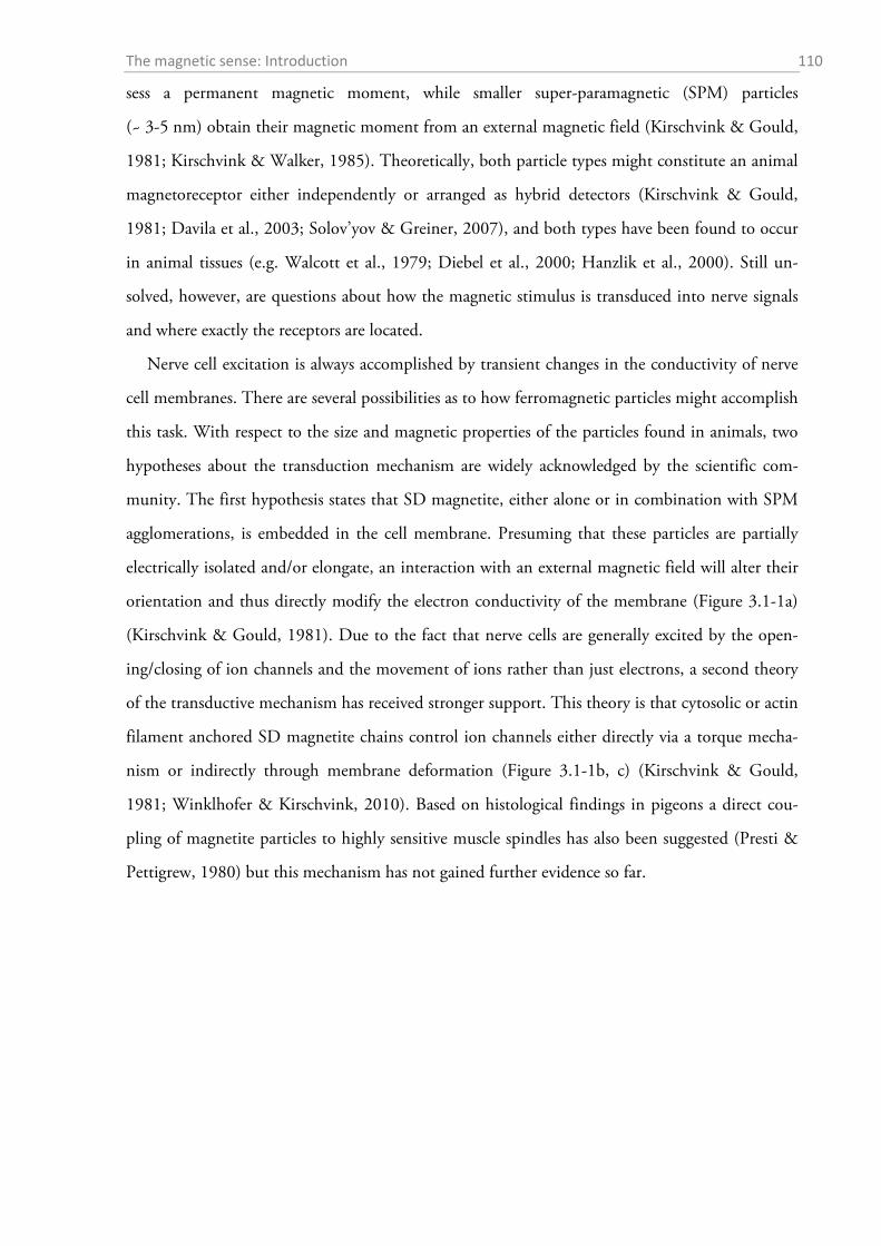
The magnetic sense: Introduction 110
sess a permanent magnetic moment, while smaller super-paramagnetic (SPM) particles
(~ 3-5 nm) obtain their magnetic moment from an external magnetic field (Kirschvink & Gould,
1981; Kirschvink & Walker, 1985). Theoretically, both particle types might constitute an animal
magnetoreceptor either independently or arranged as hybrid detectors (Kirschvink & Gould,
1981; Davila et al., 2003; Solov’yov & Greiner, 2007), and both types have been found to occur
in animal tissues (e.g. Walcott et al., 1979; Diebel et al., 2000; Hanzlik et al., 2000). Still un-
solved, however, are questions about how the magnetic stimulus is transduced into nerve signals
and where exactly the receptors are located.
Nerve cell excitation is always accomplished by transient changes in the conductivity of nerve
cell membranes. There are several possibilities as to how ferromagnetic particles might accomplish
this task. With respect to the size and magnetic properties of the particles found in animals, two
hypotheses about the transduction mechanism are widely acknowledged by the scientific com-
munity. The first hypothesis states that SD magnetite, either alone or in combination with SPM
agglomerations, is embedded in the cell membrane. Presuming that these particles are partially
electrically isolated and/or elongate, an interaction with an external magnetic field will alter their
orientation and thus directly modify the electron conductivity of the membrane (Figure 3.1-1a)
(Kirschvink & Gould, 1981). Due to the fact that nerve cells are generally excited by the open-
ing/closing of ion channels and the movement of ions rather than just electrons, a second theory
of the transductive mechanism has received stronger support. This theory is that cytosolic or actin
filament anchored SD magnetite chains control ion channels either directly via a torque mecha-
nism or indirectly through membrane deformation (Figure 3.1-1b, c) (Kirschvink & Gould,
1981; Winklhofer & Kirschvink, 2010). Based on histological findings in pigeons a direct cou-
pling of magnetite particles to highly sensitive muscle spindles has also been suggested (Presti &
Pettigrew, 1980) but this mechanism has not gained further evidence so far.
The magnetic sense: Introduction 111
Figure 3.1-1 Three suggested models of the cellular signal transduction in a magnetite based mechanism of magnetoreception. (a) The membrane-short model. An elongated magnetite particle is embedded in the cell mem-brane. The particle is partially isolated (black layer) and aligns within a superimposed magnetic field. Only in a cer-tain alignment, the particle creates an electric shortcut which leads to de- or hyperpolarization of the cell. (b) The torque-transducer model. A chain of SD-magnetite particles is anchored at the cell membrane. The tip of the chain is connected to several gaiting filaments, which control the flow of intermembrane ion channels (note that only one channel is exemplified in the figure). Depending on the direction of the magnetic field, the chain is variably deflected and opens ion channels while closing others, ultimately changing the membrane potential. (c) The membrane de-formation model. A magnetite cluster exerts a pressure on the cellular membrane and deforms it in a manner that is dependent on the alignment of the cluster with respect to an external magnetic field. The deformation directly opens or closes ion channels. The figure is not drawn to scale. (a) After Kirschvink and Gould (1981); (b) after Walker, Dennis, and Kirschvink (2002), and Winklhofer and Kirschvink (2010); (c) after Solov’yov and Greiner (2007). The figure has already been published in Begall, Burda, Malkemper (2014).
Yet another mechanism for magnetite magnetoreception has been proposed by Edmonds (1996).
According to his idea, a group of SD-magnetite particles is embedded in a liquid crystal of a pho-
toreceptor. Within this crystal the SD-particles will be able to rotate freely and align with super-
imposed magnetic fields. The model further assumes that the liquid crystal also contains dye mol-
ecules with anisotropic absorption (e.g. carotenoids), which means that they absorb light only
The magnetic sense: Introduction 112
under a specific angle of incidence. The oil droplets that are found in the cones of some birds and
reptiles fulfill these requirements (Goldsmith et al., 1984; Edmonds, 1996). With this arrange-
ment of magnetite and pigments, light of the wavelength-band absorbed by the pigment would
only reach the photoreceptor if the cone is aligned parallel or anti-parallel to the magnetic field
lines. Many behavioural findings on magnetoreception in birds, such as its strong wavelength de-
pendency (Wiltschko & Wiltschko, 2001), could be explained by the liquid crystal mechanism.
However, so far it lacks one crucial aspect: magnetic particles have not been found in oil droplets.
Furthermore, within the scope of this review the mechanism seems even more unlikely, since
mammalian cones do not possess oil droplets (Kelber et al., 2003).
For mammals, aside from the detailed realization of the transduction mechanism, a bulk of
behavioural and histological data supports the involvement of ferromagnetic particles in the mag-
netic sense. Firstly, as mentioned above, magnetite has been demonstrated to occur in many
mammals, but this finding alone does not prove anything about its significance.
An SD magnetite magnetoreceptor enables an animal to perceive the polarity of the magnetic
field and is insensitive to low intensity oscillating magnetic fields in the MHz-range (radiofre-
quency; RF). In contrast, RF magnetic fields do interfere with radical pairs (Henbest et al.,
2004b; Ritz et al., 2004), thus disabling a radical-pair mechanism (see next section). In addition,
SD magnetite receptors have a unidirectional permanent magnetic moment and their polarity can
be flipped by a short but strong magnetic pulse (Kalmijn & Blakemore, 1978). Each of these in-
trinsic and delimiting properties can be exploited in behavioural experiments to determine
whether magnetite receptors are involved.
The first experimental paradigm that yielded replicable, reliable results, and thus could be used
to investigate the properties of the magnetoreceptor in a mammal, was the nest-building assay
with mole-rats of the genus Fukomys (cf. 2.4). When mole-rats were treated with a strong magnet-
ic pulse prior to testing, they changed the direction of their nest-building preference by 90°, an
effect that lasted for several weeks (Marhold, et al., 1997). A long lasting effect of pulse treatment
is in accordance with the SD character of magnetite particles – but since no recovery from the
effect was reported in the mole-rat experiment, unspecific effects on the receptors cannot be ruled
out. However, the same authors showed that mole-rats respond to the polarity of the magnetic
field rather than to its inclination (Marhold, et al., 1997a, 1997b) and both of these findings
combined strongly suggest the involvement of SD magnetite.
The magnetic sense: Introduction 113
Sensitivity to the polarity of the magnetic field was subsequently demonstrated in another sub-
terranean rodent species, the blind mole-rat Spalax ehrenbergi (Kimchi & Terkel, 2001). Two
epigeic rodents, the Siberian hamster Phodopus sungorus and laboratory C57Bl/6J mice, have also
shown clear magnetic orientation but the experiments performed so far do not allow any conclu-
sive statement about the underlying receptor mechanism (Deutschlander et al., 2003; Muheim et
al., 2006). The latter is also true for the controversial homing experiments on the European wood
mouse (Mather & Baker, 1981).
Even though pulsing experiments had indicated magnetite as the basis of magnetoreception in
mole-rats, it took almost 10 years until the possible localization of the magnetoreceptor cells was
shown by an elegant combination of histological and behavioural investigations. Here, in spite of
the fact that the subterranean mole-rats have strongly reduced eyes, iron staining (Prussian blue)
revealed small particles in the corneal epithelium (Wegner et al., 2006). Congruently with an in-
volvement of these particles in magnetoreception, corneal anesthesia abolished the natural prefer-
ence of the animals to build nests in the south-eastern sector of a circular arena. As opposed to
sham-treated control animals, the nests of the anesthetized animals were randomly distributed
even though the visual sense was not impaired by the treatment (Wegner et al., 2006). In agree-
ment with comparable impairment of magnetoreception in beak-anaesthetized birds (Wiltschko
et al., 2009), these findings on the cornea constitute the best evidence for the seat of the mamma-
lian magnetoreceptors so far. Moreover, the mammalian cornea is innervated by the trigeminal
nerve, which has also been proposed to carry sensory information from (magnetite-based) magne-
toreceptors in birds (e.g. Mora et al., 2004; Heyers et al., 2010; Wu & Dickman, 2011; but see
Treiber et al., 2012; Wu & Dickman, 2012). Finally, neuronal activation studies in mole-rats
revealed magnetic field-dependent activity in a layer of the superior colliculus that dominantly
receives trigeminal input (Němec et al., 2001).
Bats, the only group of non-rodent mammals studied in this respect so far, also use a polarity
compass rather than an inclination compass (Wang et al., 2007). In accordance with this, pulsing
also disrupted the homeward orientation of displaced big brown bats Eptesicus fuscus (Holland et
al., 2008).
To sum up, magnetite-based magnetoreception is a highly promising candidate in mammals.
All species that have been specifically tested so far responded to the polarity of the magnetic field
and are disturbed by magnetic pulses but not by weak RF-fields (see below). However, this
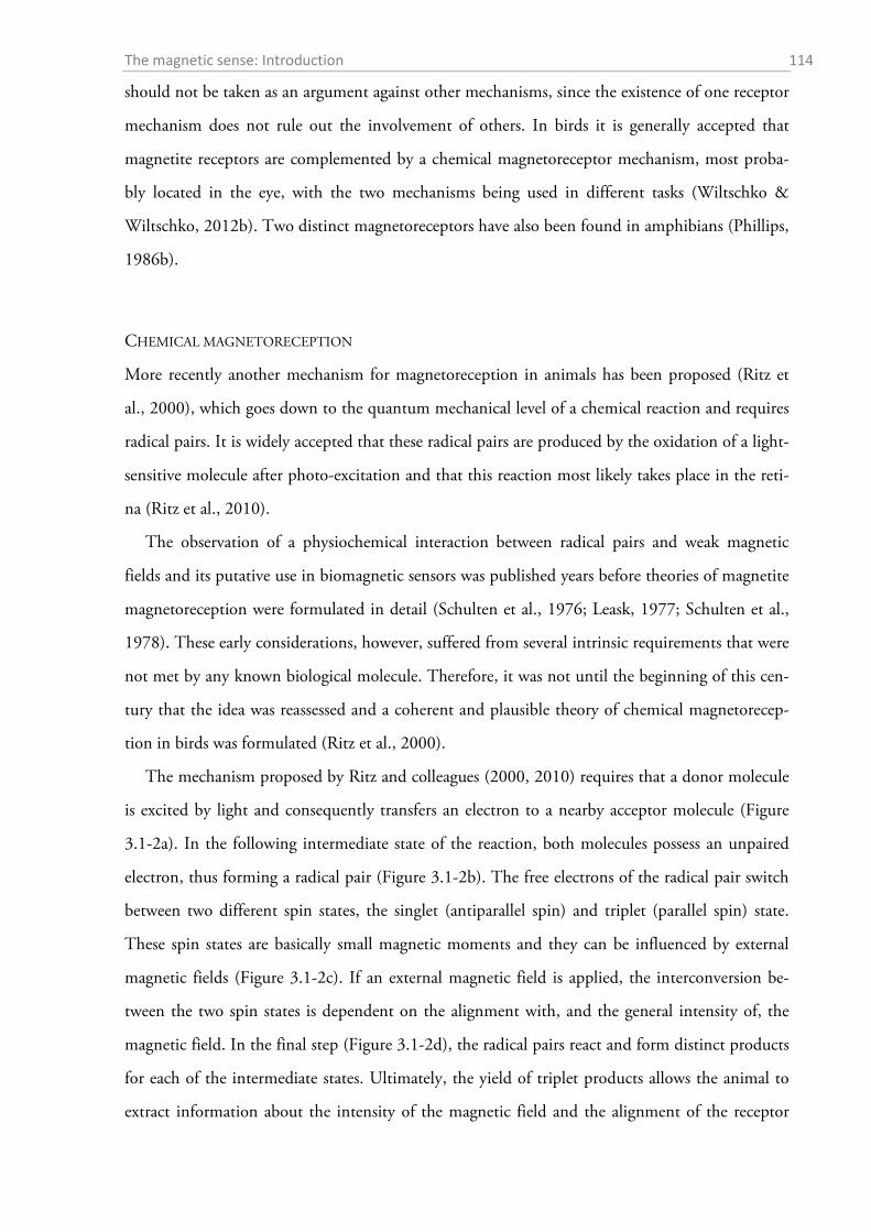
The magnetic sense: Introduction 114
should not be taken as an argument against other mechanisms, since the existence of one receptor
mechanism does not rule out the involvement of others. In birds it is generally accepted that
magnetite receptors are complemented by a chemical magnetoreceptor mechanism, most proba-
bly located in the eye, with the two mechanisms being used in different tasks (Wiltschko &
Wiltschko, 2012b). Two distinct magnetoreceptors have also been found in amphibians (Phillips,
1986b).
CHEMICAL MAGNETORECEPTION
More recently another mechanism for magnetoreception in animals has been proposed (Ritz et
al., 2000), which goes down to the quantum mechanical level of a chemical reaction and requires
radical pairs. It is widely accepted that these radical pairs are produced by the oxidation of a light-
sensitive molecule after photo-excitation and that this reaction most likely takes place in the reti-
na (Ritz et al., 2010).
The observation of a physiochemical interaction between radical pairs and weak magnetic
fields and its putative use in biomagnetic sensors was published years before theories of magnetite
magnetoreception were formulated in detail (Schulten et al., 1976; Leask, 1977; Schulten et al.,
1978). These early considerations, however, suffered from several intrinsic requirements that were
not met by any known biological molecule. Therefore, it was not until the beginning of this cen-
tury that the idea was reassessed and a coherent and plausible theory of chemical magnetorecep-
tion in birds was formulated (Ritz et al., 2000).
The mechanism proposed by Ritz and colleagues (2000, 2010) requires that a donor molecule
is excited by light and consequently transfers an electron to a nearby acceptor molecule (Figure
3.1-2a). In the following intermediate state of the reaction, both molecules possess an unpaired
electron, thus forming a radical pair (Figure 3.1-2b). The free electrons of the radical pair switch
between two different spin states, the singlet (antiparallel spin) and triplet (parallel spin) state.
These spin states are basically small magnetic moments and they can be influenced by external
magnetic fields (Figure 3.1-2c). If an external magnetic field is applied, the interconversion be-
tween the two spin states is dependent on the alignment with, and the general intensity of, the
magnetic field. In the final step (Figure 3.1-2d), the radical pairs react and form distinct products
for each of the intermediate states. Ultimately, the yield of triplet products allows the animal to
extract information about the intensity of the magnetic field and the alignment of the receptor
The magnetic sense: Introduction 115
molecules with respect to the magnetic field lines. In particular, the critical transition between the
spin states can specifically be affected through resonance effects with weak (nT-range) oscillating
magnetic fields in the range between 0.1-10 MHz, a property that can be utilized as a diagnostic
tool in behavioural experiments (Ritz et al., 2004).
Figure 3.1-2 A simplified scheme of the radical-pair mechanism of magnetoreception. (a) A donor molecule (D) is excited by light (of specific wavelengths) and subsequently transfers an electron to a nearby acceptor molecule (A). (b) This leads to the generation of a radical pair where both molecules possess a single unpaired electron. (c) The unpaired electrons of both radical-pair partners can exist in two different states (singlet and triplet). Depending on the intensity and direction of an external magnetic field, the interconversion between the states is shifted to one di-rection. (d) The switching state of the radical-pair spin state leads to varying yields of respective products. The com-parison of the product yield enables the animal to extract information about the parameters of the magnetic field. Modified from Ritz et al. (2009). The figure has already been published in Begall, Burda, Malkemper (2014).
Cryptochrome, a blue-light sensitive photoreceptor molecule, is at present the most promising
candidate for the magnetoreceptor (Ritz et al., 2000, 2010; Liedvogel & Mouritsen, 2010). It is
present in cells of a variety of plant and animal species, including mammals, where it is known to
be responsible for the maintenance of circadian rhythms (Cashmore et al., 1999; Horst et al.,
1999). The orbital arrangement of the retinal cells fulfils a critical prerequisite for the radical-pair
compass to work: the cryptochrome molecules of the different cells are aligned into distinct direc-
tions (Ritz et al., 2000). If we further assume that within any sensory cell the alignment of the
cryptochrome molecules is uniform, the triplet product yield at any given moment will vary
across the retina. This pattern is believed to be perceived by the animal as a light-dark pattern su-
perimposed on the normal visual scene (Ritz et al., 2000; Solov'yov et al., 2010). The pattern is
complex but axially symmetrical, which means that if an animal is looking parallel to the field
The magnetic sense: Introduction 116
lines it cannot distinguish between “looking north” and “looking south”. This is in accordance
with the behaviour of migratory birds, which also do not respond to a change in the polarity of
the magnetic field but rather to its inclination (Wiltschko & Wiltschko, 1972).
The description of the radical-pair mechanism given above is a rather simplified and general
version of a very complex model. The simplification was chosen on the one hand in consideration
of the scope of this thesis but also and importantly because many basic parameters of the reaction
mechanism are still unclear. For example, it is not resolved what exactly is the signalling state of
cryptochrome in animals (Nießner et al., 2013), which radical-pairs are involved and essential for
magnetoreception (Ritz et al., 2009; Müller & Ahmad, 2011), which anisotropy accounts for the
directional sensitivity of the radical-pair (Lambert et al., 2013), or whether the chemical or physi-
cal properties of the radical-pair are responsible for the sensation (Stoneham et al., 2012).
In mammals, no direct evidence for the use of a radical-pair based mechanism of magnetore-
ception exists so far. For mole-rats, in addition to the above-mentioned findings that indicate a
magnetite magnetoreceptor (pulse effect, response to polarity), experiments with radiofrequency
oscillating fields did not affect the directional preference in the nest-building assay (Thalau et al.,
2006). This indicates that mole-rats either do not possess a light-dependent radical-pair based
magnetoreceptor, which would make sense in a lightless subterranean environment (cf. Moritz et
al., 2007), or that they do not use it in the nest-building task.
For epigeic rodents, there are some indirect clues that hint towards the existence of a radical-
pair based magnetoreceptor. The first is related to the complexity and the axial symmetry of the
visual pattern that is assumed to be created by the retinal magnetoreceptors. Mice that were
trained to build their nests in one of the four cardinal magnetic directions behaved differently
when they were trained to build in N or S than when they were trained to build in E or W.
While the nests of N-S mice were clustered in the trained direction, the nests of E-W mice
formed two distinct clusters around the trained direction (Muheim et al., 2006; Painter et al.,
2013). This discrepancy suggests the perception of a complex pattern, rather than a simple com-
pass direction (Painter et al., 2013).
Further indirect evidence for the involvement of radical pairs in mammal magnetic orientation
stems from very recent findings of mouse water-maze experiments. Mice in a plus water-maze
task can quickly be trained to search for a hidden platform in a specific magnetic direction
(Phillips et al., 2013). Yet, before these elegant experiments yielded stable results the authors had
The magnetic sense: Introduction 117
to struggle with a variety of confounding factors. One of these factors were RF fields between 0.2
and 200 MHz, which had to be significantly lowered inside the test buildings for the mice to be
reliably oriented (Phillips et al., 2013). The authors state that these precautions were also crucial
for the experiments on mice and hamster nest-building published earlier (Madden & Phillips,
1987; Phillips & Deutschlander, 1997b; Deutschlander et al., 2003; Muheim et al., 2006;
Phillips et al., 2013). If the mice were using a magnetite-based mechanism for these tasks, the
weak RF magnetic fields that are typical of laboratory environments would not have had any ef-
fect.
Early experiments on pineal physiology that indicated involvement of the retina in rodent
magnetoreception fit well to the suggestion of an RPM in mammals (reviewed in Olcese, 1990).
A single 30-min change in the ambient magnetic field during the night resulted in a depression of
pineal melatonin synthesis in rats (Welker et al., 1983). This effect was abolished when the rats’
optic nerves were cut before the MF-treatment, thus indicating retinal involvement (Olcese et al.,
1985). A later study confirmed that this effect was indeed light-dependent as rats kept under dim
red light were sensitive to the effect, in contrast to rats kept in total darkness (Reuss & Olcese,
1986).
Interestingly, the MF effect was also abolished by degeneration of the outer segments of the rat
photoreceptors (Olcese et al., 1988), a region which in birds contains activated cryptochrome 1a
under influence of light of specific wavelengths, such that it strongly suggests its involvement in
magnetoreception (Nießner et al., 2011; Nießner et al., 2013). Yet the results remain puzzling,
since even though they prove the light dependency of the MF-effect, they are not consistent with
the behavioural results in migratory birds, which were disoriented in dim red light of comparable
intensity (Wiltschko et al., 1993). The presence of a cryptochrome-based system that mediates
magnetosensitivity via two antagonistic channels, as has been proposed for amphibians by Phillips
and Borland (1992), would resolve this inconsistency. At least on a theoretical level the observa-
tions are also explicable with a receptor based on magnetite particles suspended in nematic liquid
crystals as proposed by Edmonds (1996), if suitable liquid crystals could be found in mammalian
retinae. Finally, doubts have been raised about the magnetosensitivity of the pineal gland in the
rat experiments, since the effects are most likely the result of induced currents through the rapid
switching of the magnetic field (Lerchl et al., 1991). However, this does not rule out the possibil-
ity that retinal magnetoreceptors were the site of action (Phillips & Deutschlander, 1997a).
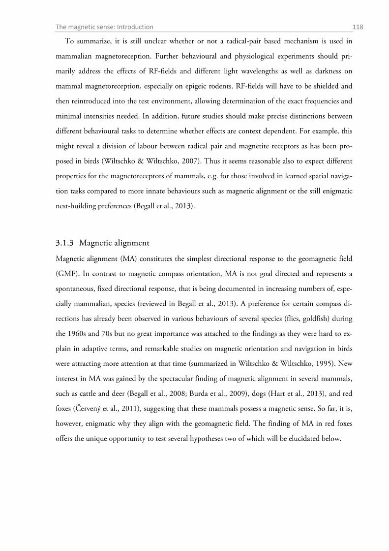
The magnetic sense: Introduction 118
To summarize, it is still unclear whether or not a radical-pair based mechanism is used in
mammalian magnetoreception. Further behavioural and physiological experiments should pri-
marily address the effects of RF-fields and different light wavelengths as well as darkness on
mammal magnetoreception, especially on epigeic rodents. RF-fields will have to be shielded and
then reintroduced into the test environment, allowing determination of the exact frequencies and
minimal intensities needed. In addition, future studies should make precise distinctions between
different behavioural tasks to determine whether effects are context dependent. For example, this
might reveal a division of labour between radical pair and magnetite receptors as has been pro-
posed in birds (Wiltschko & Wiltschko, 2007). Thus it seems reasonable also to expect different
properties for the magnetoreceptors of mammals, e.g. for those involved in learned spatial naviga-
tion tasks compared to more innate behaviours such as magnetic alignment or the still enigmatic
nest-building preferences (Begall et al., 2013).
3.1.3 Magnetic alignment
Magnetic alignment (MA) constitutes the simplest directional response to the geomagnetic field
(GMF). In contrast to magnetic compass orientation, MA is not goal directed and represents a
spontaneous, fixed directional response, that is being documented in increasing numbers of, espe-
cially mammalian, species (reviewed in Begall et al., 2013). A preference for certain compass di-
rections has already been observed in various behaviours of several species (flies, goldfish) during
the 1960s and 70s but no great importance was attached to the findings as they were hard to ex-
plain in adaptive terms, and remarkable studies on magnetic orientation and navigation in birds
were attracting more attention at that time (summarized in Wiltschko & Wiltschko, 1995). New
interest in MA was gained by the spectacular finding of magnetic alignment in several mammals,
such as cattle and deer (Begall et al., 2008; Burda et al., 2009), dogs (Hart et al., 2013), and red
foxes (Červený et al., 2011), suggesting that these mammals possess a magnetic sense. So far, it is,
however, enigmatic why they align with the geomagnetic field. The finding of MA in red foxes
offers the unique opportunity to test several hypotheses two of which will be elucidated below.
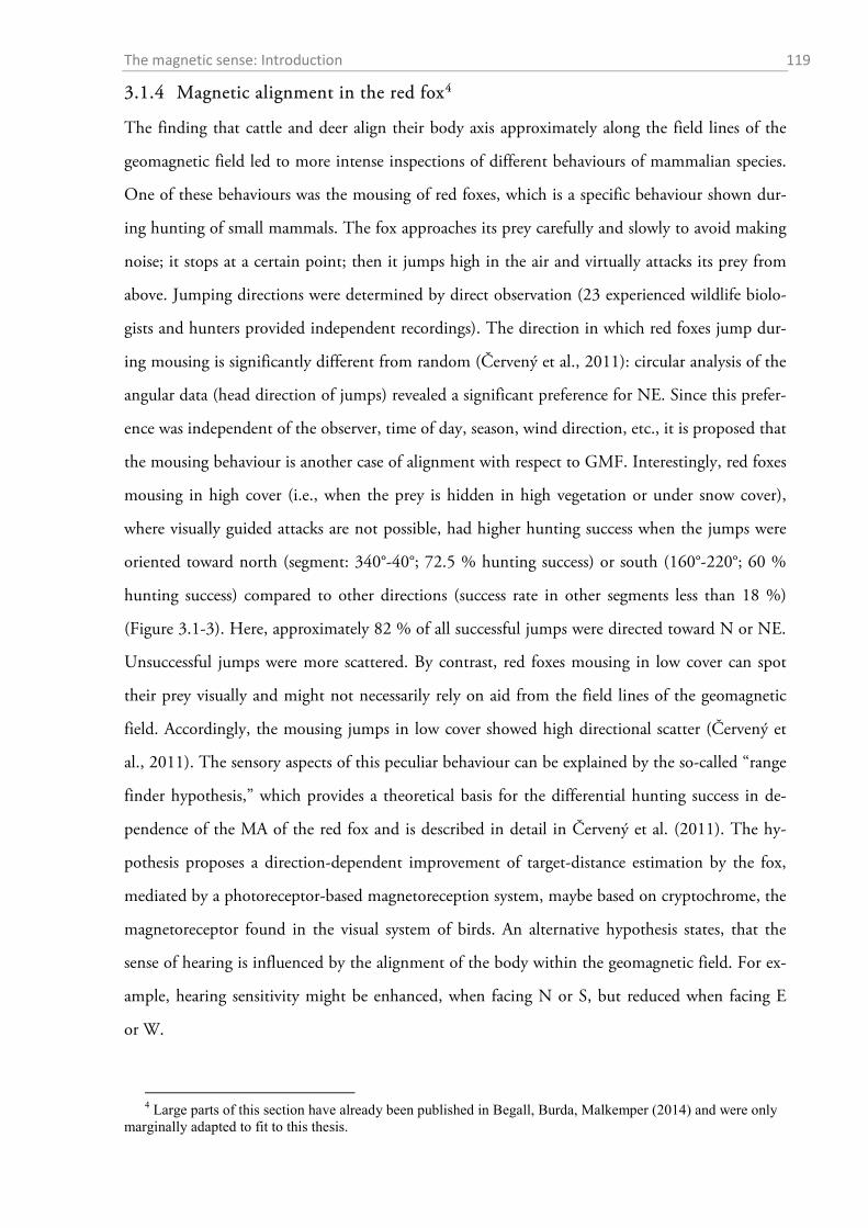
The magnetic sense: Introduction 119
3.1.4 Magnetic alignment in the red fox4
The finding that cattle and deer align their body axis approximately along the field lines of the
geomagnetic field led to more intense inspections of different behaviours of mammalian species.
One of these behaviours was the mousing of red foxes, which is a specific behaviour shown dur-
ing hunting of small mammals. The fox approaches its prey carefully and slowly to avoid making
noise; it stops at a certain point; then it jumps high in the air and virtually attacks its prey from
above. Jumping directions were determined by direct observation (23 experienced wildlife biolo-
gists and hunters provided independent recordings). The direction in which red foxes jump dur-
ing mousing is significantly different from random (Červený et al., 2011): circular analysis of the
angular data (head direction of jumps) revealed a significant preference for NE. Since this prefer-
ence was independent of the observer, time of day, season, wind direction, etc., it is proposed that
the mousing behaviour is another case of alignment with respect to GMF. Interestingly, red foxes
mousing in high cover (i.e., when the prey is hidden in high vegetation or under snow cover),
where visually guided attacks are not possible, had higher hunting success when the jumps were
oriented toward north (segment: 340°-40°; 72.5 % hunting success) or south (160°-220°; 60 %
hunting success) compared to other directions (success rate in other segments less than 18 %)
(Figure 3.1-3). Here, approximately 82 % of all successful jumps were directed toward N or NE.
Unsuccessful jumps were more scattered. By contrast, red foxes mousing in low cover can spot
their prey visually and might not necessarily rely on aid from the field lines of the geomagnetic
field. Accordingly, the mousing jumps in low cover showed high directional scatter (Červený et
al., 2011). The sensory aspects of this peculiar behaviour can be explained by the so-called “range
finder hypothesis,” which provides a theoretical basis for the differential hunting success in de-
pendence of the MA of the red fox and is described in detail in Červený et al. (2011). The hy-
pothesis proposes a direction-dependent improvement of target-distance estimation by the fox,
mediated by a photoreceptor-based magnetoreception system, maybe based on cryptochrome, the
magnetoreceptor found in the visual system of birds. An alternative hypothesis states, that the
sense of hearing is influenced by the alignment of the body within the geomagnetic field. For ex-
ample, hearing sensitivity might be enhanced, when facing N or S, but reduced when facing E
or W.
4 Large parts of this section have already been published in Begall, Burda, Malkemper (2014) and were only
marginally adapted to fit to this thesis.
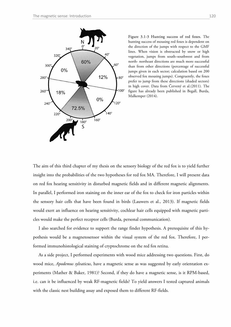
The magnetic sense: Introduction 120
Figure 3.1-3 Hunting success of red foxes. The hunting success of mousing red foxes is dependent on the direction of the jumps with respect to the GMF lines. When vision is obstructed by snow or high vegetation, jumps from south–southwest and from north- northeast directions are much more successful than from other directions (percentage of successful jumps given in each sector; calculation based on 200 observed fox mousing jumps). Congruently, the foxes prefer to jump from these directions (shaded sectors) in high cover. Data from Červený et al.(2011). The figure has already been published in Begall, Burda, Malkemper (2014).
The aim of this third chapter of my thesis on the sensory biology of the red fox is to yield further
insight into the probabilities of the two hypotheses for red fox MA. Therefore, I will present data
on red fox hearing sensitivity in disturbed magnetic fields and in different magnetic alignments.
In parallel, I performed iron staining on the inner ear of the fox to check for iron particles within
the sensory hair cells that have been found in birds (Lauwers et al., 2013). If magnetic fields
would exert an influence on hearing sensitivity, cochlear hair cells equipped with magnetic parti-
cles would make the perfect receptor cells (Burda, personal communication).
I also searched for evidence to support the range finder hypothesis. A prerequisite of this hy-
pothesis would be a magnetosensor within the visual system of the red fox. Therefore, I per-
formed immunohistological staining of cryptochrome on the red fox retina.
As a side project, I performed experiments with wood mice addressing two questions. First, do
wood mice, Apodemus sylvaticus, have a magnetic sense as was suggested by early orientation ex-
periments (Mather & Baker, 1981)? Second, if they do have a magnetic sense, is it RPM-based,
i.e. can it be influenced by weak RF-magnetic fields? To yield answers I tested captured animals
with the classic nest building assay and exposed them to different RF-fields.
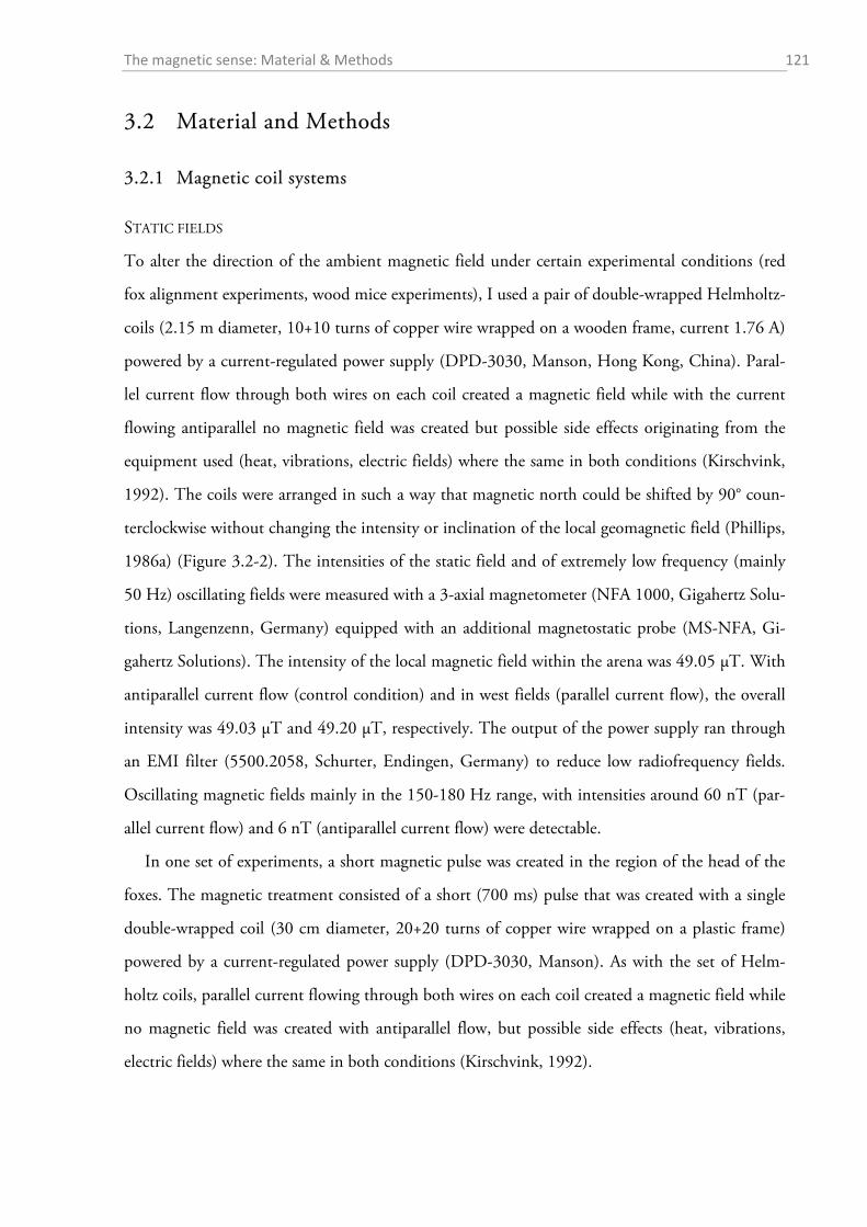
The magnetic sense: Material & Methods 121
3.2 Material and Methods
3.2.1 Magnetic coil systems
STATIC FIELDS
To alter the direction of the ambient magnetic field under certain experimental conditions (red
fox alignment experiments, wood mice experiments), I used a pair of double-wrapped Helmholtz-
coils (2.15 m diameter, 10+10 turns of copper wire wrapped on a wooden frame, current 1.76 A)
powered by a current-regulated power supply (DPD-3030, Manson, Hong Kong, China). Paral-
lel current flow through both wires on each coil created a magnetic field while with the current
flowing antiparallel no magnetic field was created but possible side effects originating from the
equipment used (heat, vibrations, electric fields) where the same in both conditions (Kirschvink,
1992). The coils were arranged in such a way that magnetic north could be shifted by 90° coun-
terclockwise without changing the intensity or inclination of the local geomagnetic field (Phillips,
1986a) (Figure 3.2-2). The intensities of the static field and of extremely low frequency (mainly
50 Hz) oscillating fields were measured with a 3-axial magnetometer (NFA 1000, Gigahertz Solu-
tions, Langenzenn, Germany) equipped with an additional magnetostatic probe (MS-NFA, Gi-
gahertz Solutions). The intensity of the local magnetic field within the arena was 49.05 µT. With
antiparallel current flow (control condition) and in west fields (parallel current flow), the overall
intensity was 49.03 µT and 49.20 µT, respectively. The output of the power supply ran through
an EMI filter (5500.2058, Schurter, Endingen, Germany) to reduce low radiofrequency fields.
Oscillating magnetic fields mainly in the 150-180 Hz range, with intensities around 60 nT (par-
allel current flow) and 6 nT (antiparallel current flow) were detectable.
In one set of experiments, a short magnetic pulse was created in the region of the head of the
foxes. The magnetic treatment consisted of a short (700 ms) pulse that was created with a single
double-wrapped coil (30 cm diameter, 20+20 turns of copper wire wrapped on a plastic frame)
powered by a current-regulated power supply (DPD-3030, Manson). As with the set of Helm-
holtz coils, parallel current flowing through both wires on each coil created a magnetic field while
no magnetic field was created with antiparallel flow, but possible side effects (heat, vibrations,
electric fields) where the same in both conditions (Kirschvink, 1992).
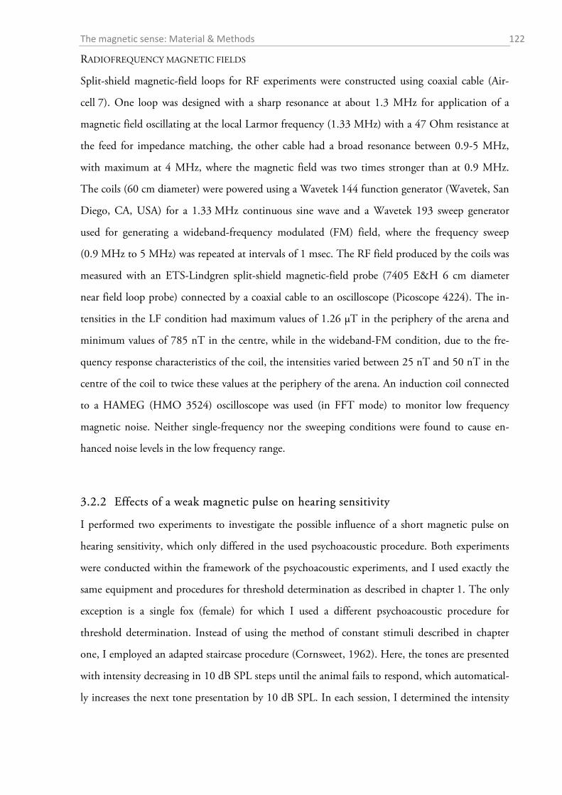
The magnetic sense: Material & Methods 122
RADIOFREQUENCY MAGNETIC FIELDS
Split-shield magnetic-field loops for RF experiments were constructed using coaxial cable (Air-
cell 7). One loop was designed with a sharp resonance at about 1.3 MHz for application of a
magnetic field oscillating at the local Larmor frequency (1.33 MHz) with a 47 Ohm resistance at
the feed for impedance matching, the other cable had a broad resonance between 0.9-5 MHz,
with maximum at 4 MHz, where the magnetic field was two times stronger than at 0.9 MHz.
The coils (60 cm diameter) were powered using a Wavetek 144 function generator (Wavetek, San
Diego, CA, USA) for a 1.33 MHz continuous sine wave and a Wavetek 193 sweep generator
used for generating a wideband-frequency modulated (FM) field, where the frequency sweep
(0.9 MHz to 5 MHz) was repeated at intervals of 1 msec. The RF field produced by the coils was
measured with an ETS-Lindgren split-shield magnetic-field probe (7405 E&H 6 cm diameter
near field loop probe) connected by a coaxial cable to an oscilloscope (Picoscope 4224). The in-
tensities in the LF condition had maximum values of 1.26 µT in the periphery of the arena and
minimum values of 785 nT in the centre, while in the wideband-FM condition, due to the fre-
quency response characteristics of the coil, the intensities varied between 25 nT and 50 nT in the
centre of the coil to twice these values at the periphery of the arena. An induction coil connected
to a HAMEG (HMO 3524) oscilloscope was used (in FFT mode) to monitor low frequency
magnetic noise. Neither single-frequency nor the sweeping conditions were found to cause en-
hanced noise levels in the low frequency range.
3.2.2 Effects of a weak magnetic pulse on hearing sensitivity
I performed two experiments to investigate the possible influence of a short magnetic pulse on
hearing sensitivity, which only differed in the used psychoacoustic procedure. Both experiments
were conducted within the framework of the psychoacoustic experiments, and I used exactly the
same equipment and procedures for threshold determination as described in chapter 1. The only
exception is a single fox (female) for which I used a different psychoacoustic procedure for
threshold determination. Instead of using the method of constant stimuli described in chapter
one, I employed an adapted staircase procedure (Cornsweet, 1962). Here, the tones are presented
with intensity decreasing in 10 dB SPL steps until the animal fails to respond, which automatical-
ly increases the next tone presentation by 10 dB SPL. In each session, I determined the intensity
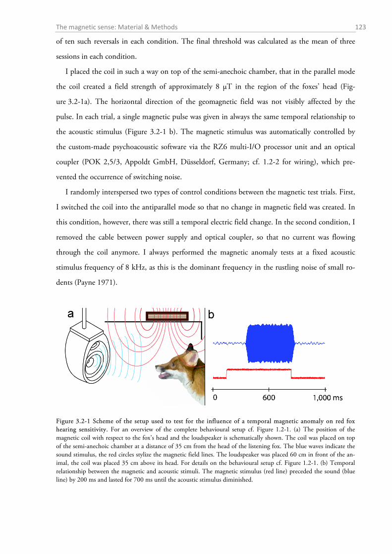
The magnetic sense: Material & Methods 123
of ten such reversals in each condition. The final threshold was calculated as the mean of three
sessions in each condition.
I placed the coil in such a way on top of the semi-anechoic chamber, that in the parallel mode
the coil created a field strength of approximately 8 µT in the region of the foxes’ head (Fig-
ure 3.2-1a). The horizontal direction of the geomagnetic field was not visibly affected by the
pulse. In each trial, a single magnetic pulse was given in always the same temporal relationship to
the acoustic stimulus (Figure 3.2-1 b). The magnetic stimulus was automatically controlled by
the custom-made psychoacoustic software via the RZ6 multi-I/O processor unit and an optical
coupler (POK 2,5/3, Appoldt GmbH, Düsseldorf, Germany; cf. 1.2-2 for wiring), which pre-
vented the occurrence of switching noise.
I randomly interspersed two types of control conditions between the magnetic test trials. First,
I switched the coil into the antiparallel mode so that no change in magnetic field was created. In
this condition, however, there was still a temporal electric field change. In the second condition, I
removed the cable between power supply and optical coupler, so that no current was flowing
through the coil anymore. I always performed the magnetic anomaly tests at a fixed acoustic
stimulus frequency of 8 kHz, as this is the dominant frequency in the rustling noise of small ro-
dents (Payne 1971).
Figure 3.2-1 Scheme of the setup used to test for the influence of a temporal magnetic anomaly on red fox hearing sensitivity. For an overview of the complete behavioural setup cf. Figure 1.2-1. (a) The position of the magnetic coil with respect to the fox’s head and the loudspeaker is schematically shown. The coil was placed on top of the semi-anechoic chamber at a distance of 35 cm from the head of the listening fox. The blue waves indicate the sound stimulus, the red circles stylize the magnetic field lines. The loudspeaker was placed 60 cm in front of the an-imal, the coil was placed 35 cm above its head. For details on the behavioural setup cf. Figure 1.2-1. (b) Temporal relationship between the magnetic and acoustic stimuli. The magnetic stimulus (red line) preceded the sound (blue line) by 200 ms and lasted for 700 ms until the acoustic stimulus diminished.
The magnetic sense: Material & Methods 124
3.2.3 Experiment on the effect of magnetic alignment on hearing sensitivity
To reveal a possible influence of the alignment between the magnetic field and the direction to-
wards the fox was listening, all behavioural experiments with male 1 described in chapter 1 were
performed within a pair of double-wrapped Helmholtz-coils that I set up around the semi-
anechoic chamber and operated in antiparallel mode (cf. section on static fields and Figure
3.2-2a, b). Additionally, for some frequencies (1 kHz, 4 kHz, 6.3 kHz, 8 kHz, and 16 kHz) the
final threshold was determined twice, once in antiparallel and once in parallel mode, the latter
rotating magnetic north towards west, leaving the red fox listening into magnetic east direction
(Figure 3.2-2a, b). The intensity of the magnetic field did not considerably differ between both
conditions (49.03 µT in antiparallel mode (control), 49.20 µT in parallel mode). To account for
effects of training and season (temperature), the test sessions with rotated magnetic north were
intermingled in between the standard test sessions. Current was flowing through the magnetic
coils in all tests, the only difference was the direction of the magnetic field.
3.2.4 Histology: Where are the magnetoreceptors?
IRON STAINING
To check for the occurrence of ferric iron particles in the sensory hair cells of the red fox inner
ear, I stained whole mounts and paraffin-celloidin sections with Prussian blue (PrB). The cochlear
whole mount preparation followed the procedures described in chapter 1, with the only differ-
ence that I used no haematoxylin and toluidine blue but instead performed the iron staining on
the intact cochlea in order to avoid staining of artifacts that might have been introduced during
the preparation. I exclusively used titanium and ceramic instruments that were rinsed in 5 % HCl
for at least 10’ before the start of the preparation.
To rinse the cochlea with PrB, I opened the bony capsule of the cochlea in the region of the
apex and the oval window and injected the PrB solution (1:1 mixture of 5 % potassium-
hexacyanoferrate and 5 % HCl) into the apical opening with a syringe. Then I submerged the
whole specimen for 30’ in the PrB solution. After staining I rinsed the cochlea with PBS and con-
tinued with the preparation as already described. I mounted the exposed half-turns in glycerol on
an untreated microscope slide.
The magnetic sense: Material & Methods 125
After the first observation and documentation at the light microscope (BX 40, Olympus), I
removed the coverslip and rinsed the cochlea thoroughly in PBS to wash away the embedding
medium. A second incubation step in PrB for another 30’ and light-microscopic documentation
followed.
Cochlear sections were prepared as described in chapter 1. To avoid contamination, I used ce-
ramic coated microtome blades (DuraEdge BLM00103P (7203) High Profile, Crescent Manu-
facturing, Fremont, OH, USA). I counterstained every second slice with nuclear fast red (NFR)
for 1-3 minutes.
CRYPTOCHROME IMMUNOHISTOCHEMISTRY
Immunostaining against Cry1 was performed together with Christine Nießner in the laboratories
of Prof. Dr. Leo Peichl at the Max-Planck-Institute for Brain Research, Frankfurt am Main,
Germany. We used the retinae of two red fox specimens and one eye of a European wood mouse.
The preparation of the retinae followed the same protocol as describe for the opsin immuno-
histochemistry in chapter 2. We processed the retinae for whole mounts free floating in a 6-well
plate before mounting them upside down onto an untreated microscope slide to promote visual
access to the photoreceptor layers after staining was completed.
Retinal sections of a red fox retina were kindly provided by Prof. Dr. Leo Peichl. The sections
originated from an adult specimen killed by a hunter. The eyes were immersion fixed in 4 % PFA
in PB for 28 h starting 30’ postmortem. 14 µm thick cryosections were prepared and stored
at -20°C until usage.
The visualization of Cry1 and S cones was accomplished by immunohistochemistry according
to the following steps (all performed at ambient temperature):
wash the fixed and prepared retina in PB (0.1M pH = 7.4; several times, if retina had
been bleached before, see chapter 2)
block with 1 ml 10 % normal donkey serum (NDS), 2 % bovine serum albumin (BSA),
0.25 % Triton-X-100 in PB for 1 h
wash in 0.1 M PB
incubate with the first antibody diluted in 1 ml 3 % NDS, 2 % BSA, 0.25 % Triton-X-
100, 0.05 % sodium azide in 0.1 M PB on a lab shaker for 3 days (sections overnight)
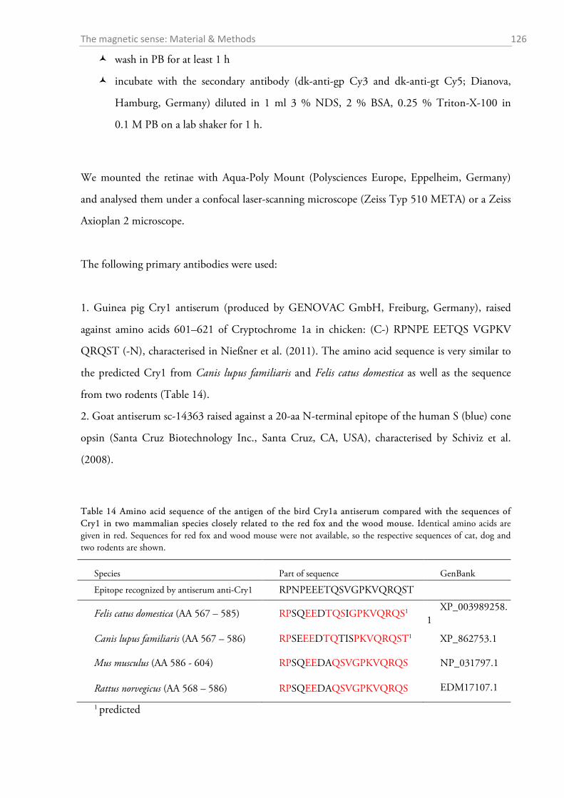
The magnetic sense: Material & Methods 126
wash in PB for at least 1 h
incubate with the secondary antibody (dk-anti-gp Cy3 and dk-anti-gt Cy5; Dianova,
Hamburg, Germany) diluted in 1 ml 3 % NDS, 2 % BSA, 0.25 % Triton-X-100 in
0.1 M PB on a lab shaker for 1 h.
We mounted the retinae with Aqua-Poly Mount (Polysciences Europe, Eppelheim, Germany)
and analysed them under a confocal laser-scanning microscope (Zeiss Typ 510 META) or a Zeiss
Axioplan 2 microscope.
The following primary antibodies were used:
1. Guinea pig Cry1 antiserum (produced by GENOVAC GmbH, Freiburg, Germany), raised
against amino acids 601–621 of Cryptochrome 1a in chicken: (C-) RPNPE EETQS VGPKV
QRQST (-N), characterised in Nießner et al. (2011). The amino acid sequence is very similar to
the predicted Cry1 from Canis lupus familiaris and Felis catus domestica as well as the sequence
from two rodents (Table 14).
2. Goat antiserum sc-14363 raised against a 20-aa N-terminal epitope of the human S (blue) cone
opsin (Santa Cruz Biotechnology Inc., Santa Cruz, CA, USA), characterised by Schiviz et al.
(2008).
Table 14 Amino acid sequence of the antigen of the bird Cry1a antiserum compared with the sequences of Cry1 in two mammalian species closely related to the red fox and the wood mouse. Identical amino acids are given in red. Sequences for red fox and wood mouse were not available, so the respective sequences of cat, dog and two rodents are shown.
Species Part of sequence GenBank
Epitope recognized by antiserum anti-Cry1 RPNPEEETQSVGPKVQRQST
Felis catus domestica (AA 567 – 585) RPSQEEDTQSIGPKVQRQS1 XP_003989258.
1
Canis lupus familiaris (AA 567 – 586) RPSEEEDTQTISPKVQRQST1 XP_862753.1
Mus musculus (AA 586 - 604) RPSQEEDAQSVGPKVQRQS NP_031797.1
Rattus norvegicus (AA 568 – 586) RPSQEEDAQSVGPKVQRQS EDM17107.1
1 predicted
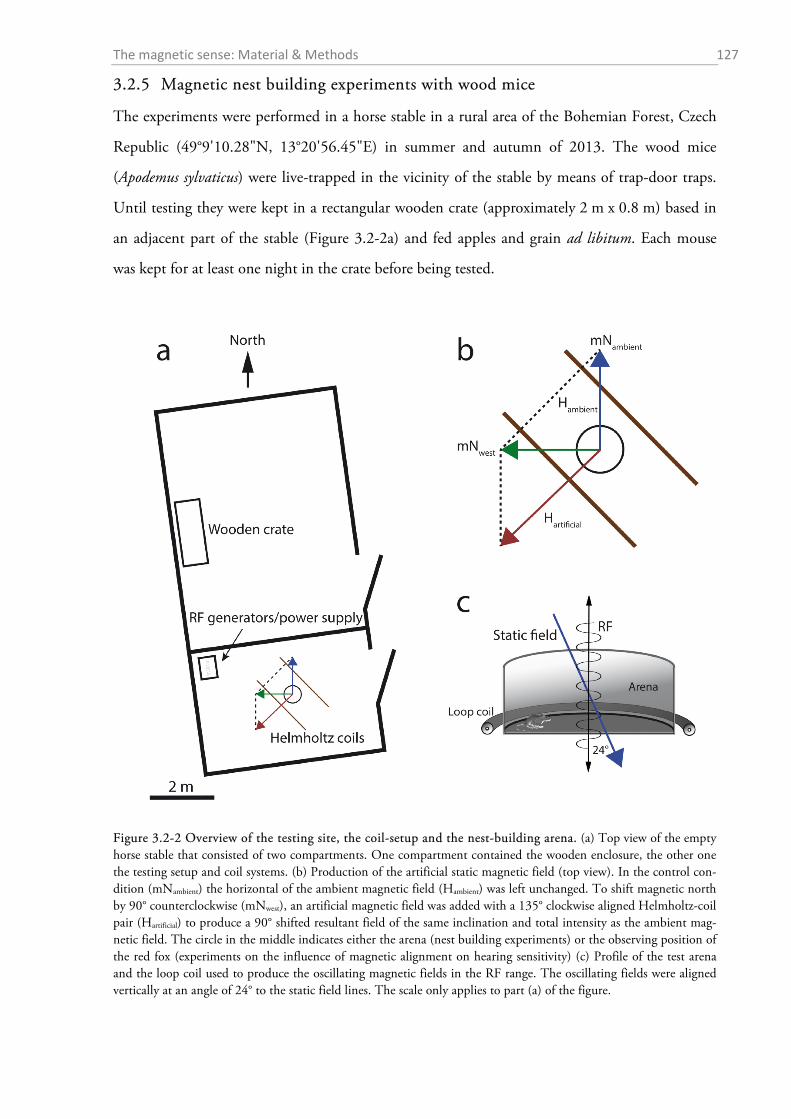
The magnetic sense: Material & Methods 127
3.2.5 Magnetic nest building experiments with wood mice
The experiments were performed in a horse stable in a rural area of the Bohemian Forest, Czech
Republic (49°9'10.28"N, 13°20'56.45"E) in summer and autumn of 2013. The wood mice
(Apodemus sylvaticus) were live-trapped in the vicinity of the stable by means of trap-door traps.
Until testing they were kept in a rectangular wooden crate (approximately 2 m x 0.8 m) based in
an adjacent part of the stable (Figure 3.2-2a) and fed apples and grain ad libitum. Each mouse
was kept for at least one night in the crate before being tested.
Figure 3.2-2 Overview of the testing site, the coil-setup and the nest-building arena. (a) Top view of the empty horse stable that consisted of two compartments. One compartment contained the wooden enclosure, the other one the testing setup and coil systems. (b) Production of the artificial static magnetic field (top view). In the control con-dition (mNambient) the horizontal of the ambient magnetic field (Hambient) was left unchanged. To shift magnetic north by 90° counterclockwise (mNwest), an artificial magnetic field was added with a 135° clockwise aligned Helmholtz-coil pair (Hartificial) to produce a 90° shifted resultant field of the same inclination and total intensity as the ambient mag-netic field. The circle in the middle indicates either the arena (nest building experiments) or the observing position of the red fox (experiments on the influence of magnetic alignment on hearing sensitivity) (c) Profile of the test arena and the loop coil used to produce the oscillating magnetic fields in the RF range. The oscillating fields were aligned vertically at an angle of 24° to the static field lines. The scale only applies to part (a) of the figure.
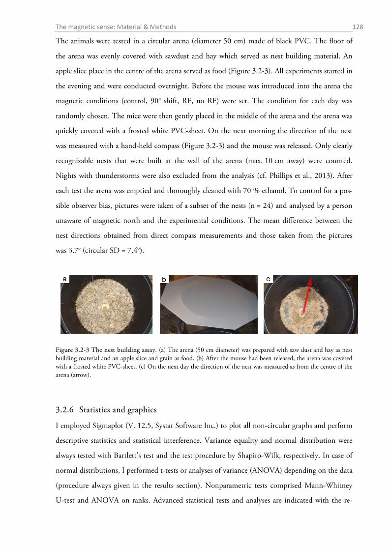
The magnetic sense: Material & Methods 128
The animals were tested in a circular arena (diameter 50 cm) made of black PVC. The floor of
the arena was evenly covered with sawdust and hay which served as nest building material. An
apple slice place in the centre of the arena served as food (Figure 3.2-3). All experiments started in
the evening and were conducted overnight. Before the mouse was introduced into the arena the
magnetic conditions (control, 90° shift, RF, no RF) were set. The condition for each day was
randomly chosen. The mice were then gently placed in the middle of the arena and the arena was
quickly covered with a frosted white PVC-sheet. On the next morning the direction of the nest
was measured with a hand-held compass (Figure 3.2-3) and the mouse was released. Only clearly
recognizable nests that were built at the wall of the arena (max. 10 cm away) were counted.
Nights with thunderstorms were also excluded from the analysis (cf. Phillips et al., 2013). After
each test the arena was emptied and thoroughly cleaned with 70 % ethanol. To control for a pos-
sible observer bias, pictures were taken of a subset of the nests (n = 24) and analysed by a person
unaware of magnetic north and the experimental conditions. The mean difference between the
nest directions obtained from direct compass measurements and those taken from the pictures
was 3.7° (circular SD = 7.4°).
Figure 3.2-3 The nest building assay. (a) The arena (50 cm diameter) was prepared with saw dust and hay as nest building material and an apple slice and grain as food. (b) After the mouse had been released, the arena was covered with a frosted white PVC-sheet. (c) On the next day the direction of the nest was measured as from the centre of the arena (arrow).
3.2.6 Statistics and graphics
I employed Sigmaplot (V. 12.5, Systat Software Inc.) to plot all non-circular graphs and perform
descriptive statistics and statistical interference. Variance equality and normal distribution were
always tested with Bartlett’s test and the test procedure by Shapiro-Wilk, respectively. In case of
normal distributions, I performed t-tests or analyses of variance (ANOVA) depending on the data
(procedure always given in the results section). Nonparametric tests comprised Mann-Whitney
U-test and ANOVA on ranks. Advanced statistical tests and analyses are indicated with the re-
The magnetic sense: Material & Methods 129
spective results in the results section. For tables, standard calculations, and data transformation I
used Excel 2010 (Microsoft Corp.). I prepared graphical illustrations in Photoshop and Illustrator
CS6 (Adobe Systems).
For analysis of the distributions of nest directions I used standard circular statistics (Batschelet,
1981). All calculations were carried out in Oriana (V. 4.02, Kovach Computing Services, Angle-
sey, Wales, UK). I treated each nest direction as an independent data point. The likelihood of
retesting a mouse was low because wood mice avoid traps for some time after they have been cap-
tured (unpublished observations). Furthermore, any mouse that was recaptured had only a 25 %
chance of being tested in the same experimental condition. For the calculation of mean vectors
the software employs simple vector addition. For axial analysis, the method of doubling the angles
was used to convert angular data in axial ones prior to statistical analysis. I used the Rayleigh test
with p < 0.05 as the threshold of statistical significance to test the data for significant deviation
from random distribution. The Watson U² test compared distributions of different experimental
groups.
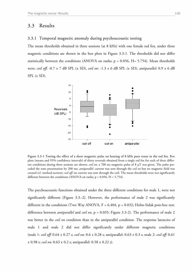
The magnetic sense: Results 130
3.3 Results
3.3.1 Temporal magnetic anomaly during psychoacoustic testing
The mean thresholds obtained in three sessions (at 8 kHz) with one female red fox, under three
magnetic conditions are shown in the box plots in Figure 3.3-1. The thresholds did not differ
statistically between the conditions (ANOVA on ranks; p = 0.056, H= 5.754). Mean thresholds
were: coil off: -0.7 ± 7 dB SPL (± SD), coil on: -1.3 ± 6 dB SPL (± SD), antiparallel: 0.9 ± 6 dB
SPL (± SD).
Figure 3.3-1 Testing the effect of a short magnetic pulse on hearing of 8 kHz pure tones in the red fox. Box plots (means and 95% confidence intervals) of thirty reversals obtained from a single red fox for each of three differ-ent conditions during three sessions are shown: coil on: a 700 ms magnetic pulse of 8 µT was given. The pulse pre-ceded the tone presentation by 200 ms; antiparallel: current was sent through the coil on but no magnetic field was created (cf. method section); coil off: no current was sent through the coil. The mean thresholds were not significantly different between the conditions (ANOVA on ranks; p = 0.056, H = 5.754).
The psychoacoustic functions obtained under the three different conditions for male 1, were not
significantly different (Figure 3.3.-2). However, the performance of male 2 was significantly
different in the conditions (Two Way ANOVA, F = 6.404, p = 0.032; Holm-Sidak post-hoc test:
difference between antiparallel and coil on, p = 0.035; Figure 3.3-2). The performance of male 2
was better in the coil on condition than in the antiparallel condition. The response latencies of
male 1 and male 2 did not differ significantly under different magnetic conditions
(male 1: coil off: 0.64 ± 0.27 s; coil on: 0.6 ± 0.28 s; antiparallel: 0.63 ± 0.3 s; male 2: coil off: 0.61
± 0.98 s; coil on: 0.63 ± 0.2 s; antiparallel: 0.58 ± 0.22 s).
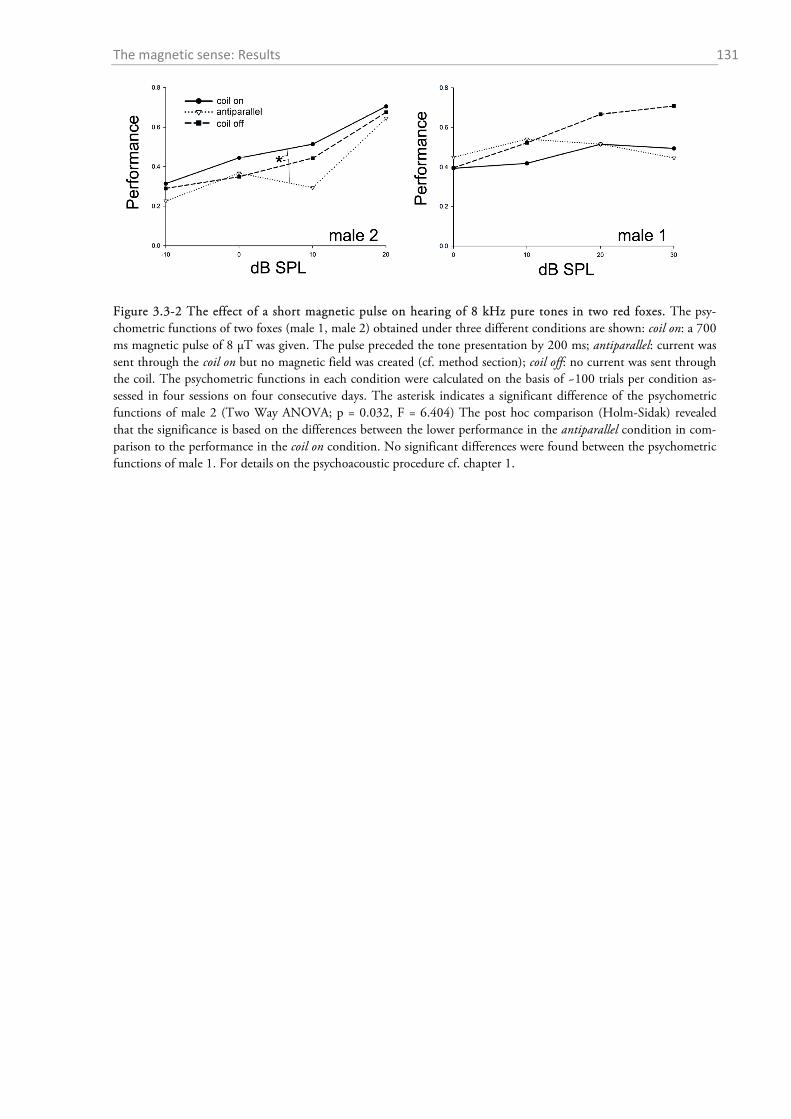
The magnetic sense: Results 131
Figure 3.3-2 The effect of a short magnetic pulse on hearing of 8 kHz pure tones in two red foxes. The psy-chometric functions of two foxes (male 1, male 2) obtained under three different conditions are shown: coil on: a 700 ms magnetic pulse of 8 µT was given. The pulse preceded the tone presentation by 200 ms; antiparallel: current was sent through the coil on but no magnetic field was created (cf. method section); coil off: no current was sent through the coil. The psychometric functions in each condition were calculated on the basis of ~100 trials per condition as-sessed in four sessions on four consecutive days. The asterisk indicates a significant difference of the psychometric functions of male 2 (Two Way ANOVA; p = 0.032, F = 6.404) The post hoc comparison (Holm-Sidak) revealed that the significance is based on the differences between the lower performance in the antiparallel condition in com-parison to the performance in the coil on condition. No significant differences were found between the psychometric functions of male 1. For details on the psychoacoustic procedure cf. chapter 1.
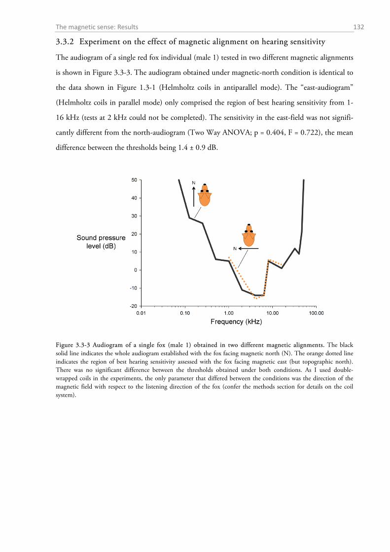
The magnetic sense: Results 132
3.3.2 Experiment on the effect of magnetic alignment on hearing sensitivity
The audiogram of a single red fox individual (male 1) tested in two different magnetic alignments
is shown in Figure 3.3-3. The audiogram obtained under magnetic-north condition is identical to
the data shown in Figure 1.3-1 (Helmholtz coils in antiparallel mode). The “east-audiogram”
(Helmholtz coils in parallel mode) only comprised the region of best hearing sensitivity from 1-
16 kHz (tests at 2 kHz could not be completed). The sensitivity in the east-field was not signifi-
cantly different from the north-audiogram (Two Way ANOVA; p = 0.404, F = 0.722), the mean
difference between the thresholds being 1.4 ± 0.9 dB.
Figure 3.3-3 Audiogram of a single fox (male 1) obtained in two different magnetic alignments. The black solid line indicates the whole audiogram established with the fox facing magnetic north (N). The orange dotted line indicates the region of best hearing sensitivity assessed with the fox facing magnetic east (but topographic north). There was no significant difference between the thresholds obtained under both conditions. As I used double-wrapped coils in the experiments, the only parameter that differed between the conditions was the direction of the magnetic field with respect to the listening direction of the fox (confer the methods section for details on the coil system).
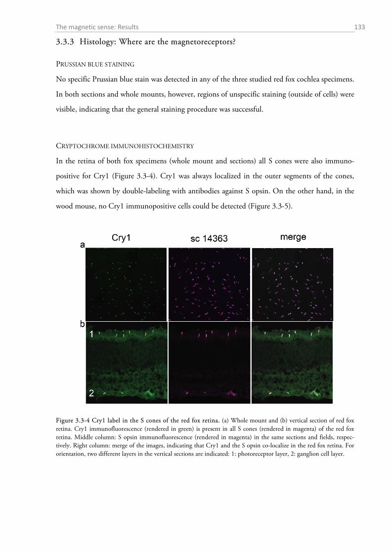
The magnetic sense: Results 133
3.3.3 Histology: Where are the magnetoreceptors?
PRUSSIAN BLUE STAINING
No specific Prussian blue stain was detected in any of the three studied red fox cochlea specimens.
In both sections and whole mounts, however, regions of unspecific staining (outside of cells) were
visible, indicating that the general staining procedure was successful.
CRYPTOCHROME IMMUNOHISTOCHEMISTRY
In the retina of both fox specimens (whole mount and sections) all S cones were also immuno-
positive for Cry1 (Figure 3.3-4). Cry1 was always localized in the outer segments of the cones,
which was shown by double-labeling with antibodies against S opsin. On the other hand, in the
wood mouse, no Cry1 immunopositive cells could be detected (Figure 3.3-5).
Figure 3.3-4 Cry1 label in the S cones of the red fox retina. (a) Whole mount and (b) vertical section of red fox retina. Cry1 immunofluorescence (rendered in green) is present in all S cones (rendered in magenta) of the red fox retina. Middle column: S opsin immunofluorescence (rendered in magenta) in the same sections and fields, respec-tively. Right column: merge of the images, indicating that Cry1 and the S opsin co-localize in the red fox retina. For orientation, two different layers in the vertical sections are indicated: 1: photoreceptor layer, 2: ganglion cell layer.
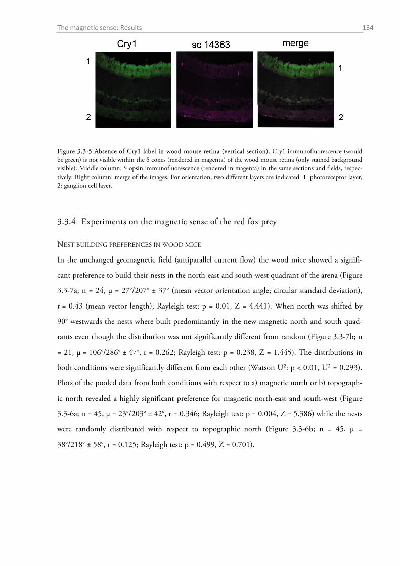
The magnetic sense: Results 134
Figure 3.3-5 Absence of Cry1 label in wood mouse retina (vertical section). Cry1 immunofluorescence (would be green) is not visible within the S cones (rendered in magenta) of the wood mouse retina (only stained background visible). Middle column: S opsin immunofluorescence (rendered in magenta) in the same sections and fields, respec-tively. Right column: merge of the images. For orientation, two different layers are indicated: 1: photoreceptor layer, 2: ganglion cell layer.
3.3.4 Experiments on the magnetic sense of the red fox prey
NEST BUILDING PREFERENCES IN WOOD MICE
In the unchanged geomagnetic field (antiparallel current flow) the wood mice showed a signifi-
cant preference to build their nests in the north-east and south-west quadrant of the arena (Figure
3.3-7a; n = 24, µ = 27°/207° ± 37° (mean vector orientation angle; circular standard deviation),
r = 0.43 (mean vector length); Rayleigh test: p = 0.01, Z = 4.441). When north was shifted by
90° westwards the nests where built predominantly in the new magnetic north and south quad-
rants even though the distribution was not significantly different from random (Figure 3.3-7b; n
= 21, µ = 106°/286° ± 47°, r = 0.262; Rayleigh test: p = 0.238, Z = 1.445). The distributions in
both conditions were significantly different from each other (Watson U²: p < 0.01, U² = 0.293).
Plots of the pooled data from both conditions with respect to a) magnetic north or b) topograph-
ic north revealed a highly significant preference for magnetic north-east and south-west (Figure
3.3-6a; n = 45, µ = 23°/203° ± 42°, r = 0.346; Rayleigh test: p = 0.004, Z = 5.386) while the nests
were randomly distributed with respect to topographic north (Figure 3.3-6b; n = 45, µ =
38°/218° ± 58°, r = 0.125; Rayleigh test: p = 0.499, Z = 0.701).
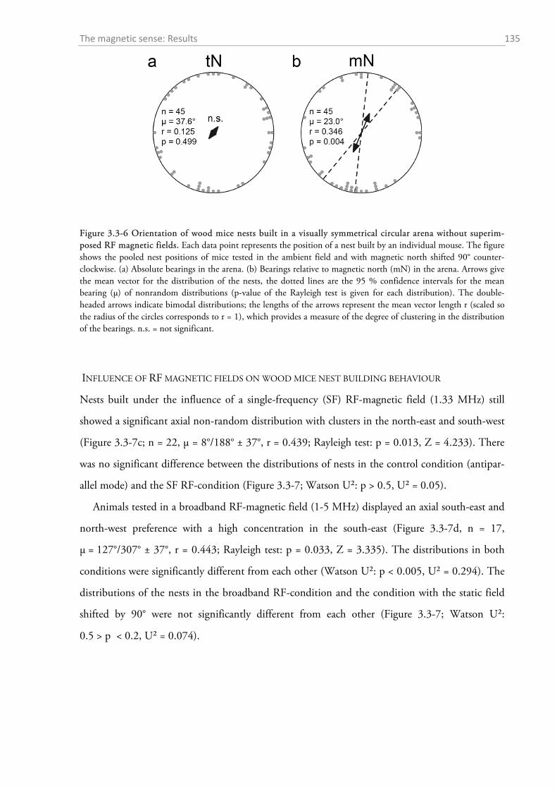
The magnetic sense: Results 135
Figure 3.3-6 Orientation of wood mice nests built in a visually symmetrical circular arena without superim-posed RF magnetic fields. Each data point represents the position of a nest built by an individual mouse. The figure shows the pooled nest positions of mice tested in the ambient field and with magnetic north shifted 90° counter-clockwise. (a) Absolute bearings in the arena. (b) Bearings relative to magnetic north (mN) in the arena. Arrows give the mean vector for the distribution of the nests, the dotted lines are the 95 % confidence intervals for the mean bearing (µ) of nonrandom distributions (p-value of the Rayleigh test is given for each distribution). The double-headed arrows indicate bimodal distributions; the lengths of the arrows represent the mean vector length r (scaled so the radius of the circles corresponds to r = 1), which provides a measure of the degree of clustering in the distribution of the bearings. n.s. = not significant.
INFLUENCE OF RF MAGNETIC FIELDS ON WOOD MICE NEST BUILDING BEHAVIOUR
Nests built under the influence of a single-frequency (SF) RF-magnetic field (1.33 MHz) still
showed a significant axial non-random distribution with clusters in the north-east and south-west
(Figure 3.3-7c; n = 22, µ = 8°/188° ± 37°, r = 0.439; Rayleigh test: p = 0.013, Z = 4.233). There
was no significant difference between the distributions of nests in the control condition (antipar-
allel mode) and the SF RF-condition (Figure 3.3-7; Watson U²: p > 0.5, U² = 0.05).
Animals tested in a broadband RF-magnetic field (1-5 MHz) displayed an axial south-east and
north-west preference with a high concentration in the south-east (Figure 3.3-7d, n = 17,
µ = 127°/307° ± 37°, r = 0.443; Rayleigh test: p = 0.033, Z = 3.335). The distributions in both
conditions were significantly different from each other (Watson U²: p < 0.005, U² = 0.294). The
distributions of the nests in the broadband RF-condition and the condition with the static field
shifted by 90° were not significantly different from each other (Figure 3.3-7; Watson U²:
0.5 > p < 0.2, U² = 0.074).
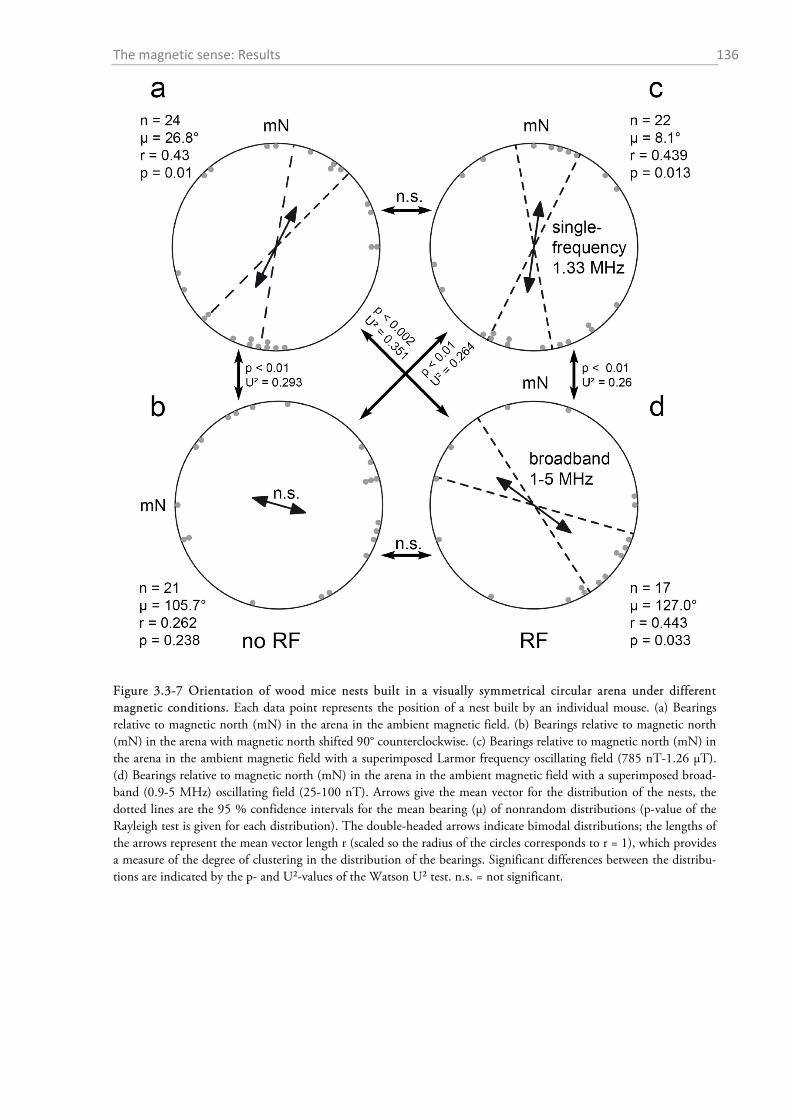
The magnetic sense: Results 136
Figure 3.3-7 Orientation of wood mice nests built in a visually symmetrical circular arena under different magnetic conditions. Each data point represents the position of a nest built by an individual mouse. (a) Bearings relative to magnetic north (mN) in the arena in the ambient magnetic field. (b) Bearings relative to magnetic north (mN) in the arena with magnetic north shifted 90° counterclockwise. (c) Bearings relative to magnetic north (mN) in the arena in the ambient magnetic field with a superimposed Larmor frequency oscillating field (785 nT-1.26 µT). (d) Bearings relative to magnetic north (mN) in the arena in the ambient magnetic field with a superimposed broad-band (0.9-5 MHz) oscillating field (25-100 nT). Arrows give the mean vector for the distribution of the nests, the dotted lines are the 95 % confidence intervals for the mean bearing (µ) of nonrandom distributions (p-value of the Rayleigh test is given for each distribution). The double-headed arrows indicate bimodal distributions; the lengths of the arrows represent the mean vector length r (scaled so the radius of the circles corresponds to r = 1), which provides a measure of the degree of clustering in the distribution of the bearings. Significant differences between the distribu-tions are indicated by the p- and U²-values of the Watson U² test. n.s. = not significant.
The magnetic sense: Discussion 137
3.4 Discussion
3.4.1 Pulse experiment
At this point it seems appropriate to clarify, that this experiment was not designed to test for the
involvement of magnetite in red fox magnetoreception, as this is the usual purpose of pulse exper-
iments in magnetoreception research (e.g. Holland et al., 2008). The pulse used here was of far
too less intensity to remagnetize single-domain magnetite and was simply intended to test for the
occurrence of magnetoreception in foxes in general.
The interpretation of the results of the pulse experiment is not straightforward. On the one
hand, statistically significant effects of the magnetic field changes were detectable in one of the
three tested foxes. On the other hand, the results do not reveal any consistencies and can at best
be interpreted as a very cautious hint that magnetoreception might exist in red foxes. Clearly,
there is no consistent or biologically relevant effect on hearing thresholds. Furthermore, since the
response latencies were not different between the conditions, foxes do not (at least not conscious-
ly) perceive the magnetic pulse, otherwise they would have had quickly learned the connection
between the reward and the magnetic stimulus, and therefore would have been expected to be-
come quicker under coil on condition with each subsequent session. In sum, the data does not
allow to conclude that the foxes’ auditory system is affected by pulsed magnetic fields. A much
larger dataset obtained in a completely acoustically shielded room might yield different results,
but would be even further away from the natural situation in the wild.
3.4.2 Horizontal shift experiment
The thresholds of the single fox listening towards magnetic north were not different from the
thresholds obtained when the fox was listening towards magnetic east. Therefore, it is highly un-
likely, that the magnetic alignment observed in hunting red foxes (Červený et al., 2011) is the
consequence of enhanced hearing sensitivity, leaving room to provide evidence for the alternative
hypotheses. One might argue that with north and east the magnetic directions were inappropri-
ately chosen, as the foxes clearly preferred the mean direction of these two, north-east and thus no
differential effect of north and east would have been expected. However, as magnetic alignment is
beginning of being recognized as a quite universally distributed phenomenon amongst mammali-
The magnetic sense: Discussion 138
an species and furthermore most species prefer the north-south axis (Begall et al., 2013), I as-
sumed that the east shift in the red fox MA would simply be based on scatter of the relatively
small sample in the study by Červený et al. (2011; at least for a MA study) and therefore decided
to test magnetic east versus magnetic north. It can, however, not be excluded that alignment with
anticardinal directions would show an effect.
Also, it is theoretically possible that only frequencies lower or higher than the tested spectrum
are affected by magnetic fields. In light of the working hypothesis that magnetic alignment influ-
ences acoustic prey detection, this would not be of relevance as the rustling noise of mice and
voles contains most energy in bands around 8-10 kHz (Payne, 1971; Konishi, 1973; Marimuthu
& Neuweiler, 1987). However, chewing noise seems to be more shifted into higher frequencies
(Payne, 1971), and future experiments should be conducted to determine whether foxes prefer
rustling or chewing noise for the detection of prey.
3.4.3 Histology: Where are the magnetoreceptors?
I was not able to demonstrate the occurrence of iron particles (cuticulosomes) in the inner ear of
the red fox by means of the Prussian blue staining of surface specimens and paraffin sections
which is in line with the absence of an effect of magnetic alignment on hearing sensitivity. It is
not a surprising finding, given that Lauwers et al. (2013) also tested several mammalian species
(rat, mice, guinea pig, human) without the appearance of any stained structures. Nevertheless, the
absence of staining does not prove that the particles do not exist, as several factors might have
complicated their discovery. First of all, the particles shown by Lauwers et al. (2013) were so
small (300-600 nm) that they might have been easily overlooked under the light microscope if
they would have been only sparsely distributed. Furthermore, it is not clear whether the Prussian
blue stain penetrates cell membranes, which might be the reason of the absence of staining in the
surface specimens. On the other hand, I could not stain every paraffin section of each cochlea (as
they were needed for the general ear morphology) and often the hair cells were disrupted or total-
ly missing. Another possibility might be related to the evolution of the auditory organ in mam-
mals. Lauwers et al (2013) demonstrated the occurrence of the iron particles in hair cells of both
the cochlear and vestibular hair cells. The sense of hearing has gained a considerably higher im-
portance during mammalian evolution that it would seem at least plausible that, assumed the par-
ticles would be sensors of magnetic fields, they might have been relocalized in order to avoid dis-
The magnetic sense: Discussion 139
turbing sensory crosstalk. As a conclusion, it still seems promising to search within the vestibular
system of the red fox.
The finding of Cry1 in the S cone outer segments of the red fox retina is a highly surprising
finding. In birds, even though the transduction process is still enigmatic, Cry1, localized with the
UV-cones of robins and chickens, is the most probable receptor molecule for the magnetic com-
pass in birds (Bischof et al., 2011; Nießner et al., 2011, 2013). The absence of staining in the
wood mouse suggests, that interspecies differences exist, which is suggestive of a rather specific
function in the red fox. Cry1 is known to be involved in circadian rhythms (Sancar, 2000), but
this seems unlikely to be the cause for cryptochromes being seated in the cone outer segments,
since for controlling circadian rhythms it needs to be able to exert influence on transcription pro-
cesses. Thus, a new role seems possible and given the findings in birds, this new role might be
magnetoreception.
At this point, however, it needs to be stated that as the experiment was preliminary and the re-
sults are only based on three specimens (two foxes, one wood mouse), not too far reaching specu-
lations should be made. Nevertheless, if shown in future that cryptochrome is involved in a mag-
netic sense of the red fox, the hypothesis of a magneto-visual range finder would gain considera-
ble new support. Furthermore, as Cry1 is exclusively found in S cones, the distribution pattern of
those and the retinal ganglion cell densities provided in this thesis, might prove very useful in de-
veloping a model of the “magnetic pattern” a fox might see, similar as it has been done in birds
(Ritz et al., 2000; Solov'yov et al., 2010).
3.4.4 Magnetic orientation in wood mice
The results provide clear evidence for a magnetic sense in wood mice. When deciding where to
build a nest in an otherwise featureless environment, the animals revealed a preference for the
magnetic north-northeast and south-southwest axis and when the alignment of the magnetic field
was rotated by 90°, the bimodal clustering of bearings, although not significant, was rotated by a
comparable extent. The increased scatter of nest positions in the 90° shifted field may have been
due to the inhomogeneity in the artificial magnetic field or, alternatively, to a cue conflict be-
tween magnetic cues and non-magnetic (e.g. sound) cues that may have been accessible for the
mice in the holding enclosure and arena. Thus, for example, the irregular creaking sound pro-
duced by the stable doors might have provided an orientation cue to the mice. During the night
The magnetic sense: Discussion 140
before the test (when the animals were kept in the enclosure) and in control condition this creak-
ing came from ~magnetic east, but from magnetic south in changed magnetic field condition (see
Figure 3.2-2a). Evidence consistent with a cue conflict between magnetic and non-magnetic cues,
and higher scatter in shifted magnetic field conditions, have been reported in other studies of ro-
dent magnetic orientation (Burda et al., 1990; Deutschlander et al., 2003; Oliveriusová et al.,
2012, 2014). Nevertheless, the results clearly confirm the presence of a magnetic sense in wood
mice, a prerequisite for a magnetic compass, which supports the findings by Mather and Baker
(Mather & Baker, 1981). A magnetic compass would be highly beneficial for nocturnal wood
mice that perform regular foraging bouts over distances of more than 200 m, show remarkable
homing ability from unfamiliar locations after displacements of up to 350 m (Hacker & Pearson,
1951; Jamon & Bovet, 1987), occupy comparatively large home ranges of 1-2 ha (Tew &
MacDonald, 1994), and show remarkable navigational strategies, including way-marking behav-
iour using portable, visual landmarks (Stopka & MacDonald, 2003).
It is unclear why mice exhibit a preference to build their nests along the magnetic ~north-
south axis, but there are two general proximate explanations: either the preference is learned (e.g.,
corresponding to the direction of some feature of the environment) or innate (consistent with
spontaneous northward magnetic orientation, or axial orientation along the north-south magnetic
axis, found in other vertebrates; Begall et al., 2013). Laboratory mice can be trained to orient in
the direction of a nest box placed at one end of the cage in which they are held prior to testing
(Muheim et al., 2006). The wood mice tested in the current study were kept in a rectangular en-
closure for up to three nights before being tested, but this pre-exposure was shorter than in earlier
studies of learned compass responses (e.g. 5-24 days in Muheim et al., 2006) and no features of
the cage environment relative to the magnetic field or to topographic cues (cage axis, shadows,
etc.) appeared to coincide with the axis of orientation exhibited by the mice. Hence it is unlikely
that the observed axial preference was learned even though “magnetic imprinting” with respect to
other cues, i.e. a response that was learned prior to the mouse being captured that was subse-
quently transferred to non-magnetic (topographic) cues, cannot be fully excluded. Also an effect
of the displacement direction cannot be ruled out as many animals were caught north-northeast
of the testing site.
Laboratory mice, in addition to showing learned compass orientation relative to the magnetic
field, also exhibit a weak, presumably innate (i.e., independent of any learned direction) axial
The magnetic sense: Discussion 141
preference along the magnetic north-south axis (Muheim et al., 2006). Recently, such a prefer-
ence was also revealed in the semi-fossorial bank vole (Clethrionomys glareolus), which
Oliveriusová et al., (2014) suggested is likely to be innate although the voles were kept in approx-
imately north-south aligned cages in the laboratory for at least 8 weeks before testing
(Oliveriusová et al., 2014). Consequently, although there is insufficient information to determine
if the observed preference in wood mice is innate or learned, it appears likely that at least some
component of the response is innate.
We can only speculate about the ultimate reasons for an innate preference to build nests along
the north-south axis of the Earth’s magnetic field. As for the more general phenomenon of mag-
netic alignment, several functions for nest position preferences seem plausible (discussed in Begall
et al., 2013). It might provide a constant directional reference for the use of a (visual) map-sense
(see below), or enhance selective attention through the facilitation of cross-modal integration
(Phillips et al., 2010). Further experiments will hopefully shed light on this issue.
3.4.5 Mechanisms of magnetoreception and the influence of RF fields
The responses of the mice under RF exposure are not straightforward to interpret in view of the
current theories on magnetoreception. The available evidence indicates that subterranean mi-
crophthalmic mole-rats rely on a light-independent MPM (Thalau et al., 2006), while the prop-
erties of learned magnetic compass orientation by epigeic rodents may point to the involvement
of a RPM (Phillips et al., 2013). It is therefore possible that macrophthalmic, epigeic wood mice
also have a RPM, in which case we expect a specific sensitivity to weak RF magnetic fields
(Henbest et al., 2004a; Ritz et al., 2004). Analogous to the experiments performed in birds and
mole-rats (Ritz et al., 2004, 2009; Thalau et al., 2006), we tested the wood mice in both Larmor
frequency (LF) and wideband-FM (comparable to broadband-RF) oscillating magnetic fields.
Contrary to the predictions of the RPM made earlier by other investigators (Ritz et al., 2004,
2009), wood mice exhibited non-random directional preferences in both conditions: The distri-
bution of bearings under the LF condition was indistinguishable from controls (i.e., nests were
bimodally distributed along the ~north-south magnetic axis; Figure 3.3-7c). In contrast, under
wideband-FM conditions it was rotated by roughly 90° relative to control. As the angle between
the static field and the RF fields was the same in both conditions (see Figure 3.2-2c), the only
differences were the overall intensity, the temporal pattern, and the frequency spectrum. The in-
The magnetic sense: Discussion 142
tensities in the LF condition had maximum values of 1.26 µT in the periphery of the arena and
minimum values of 785 nT in the centre and therefore greatly exceeded those shown to affect the
inclination compass of birds (Ritz et al., 2009; Engels et al., 2014). In the wideband-FM condi-
tion, due to the frequency response characteristics of the coil, the intensities varied between 25-50
nT in the centre of the coil to twice these values at the periphery of the arena. These field
strengths are comparable to the ones used in Engels et al. (2014), who were able to perturb the
magnetic compass of European robins by broadband electromagnetic noise with spectral intensity
of 0.1-0.2 nT per 10 kHz in the range 600 kHz-3 MHz, which upon integration over the fre-
quency domain translates into a typical RF magnetic field amplitude of 30-35 nT in the time
domain.
The fact that we observed an effect under wideband-FM field but no visible effect on nest
building under LF conditions is consistent with a RPM mechanism in which both electron spins
have an anisotropic coupling to their respective host molecules, due either to nuclear hyperfine
interactions (Schulten et al., 1978; Ritz et al., 2000) or to spin-orbit coupling (Lambert et al.,
2013). In any case, we can rule out that wood mice use a so-called optimal reference-probe RPM
model (where one of the two unpaired electrons in the radical pair - the probe spin - is devoid of
anisotropy), which was suggested by Ritz et al. (2009, 2010) to explain disorientation in birds
under very weak fields (15 nT) oscillating at the Larmor frequency. Under the assumption that
cryptochrome 1a (Nießner et al., 2011, 2013) is the responsible molecule for RPM magnetore-
ception in mammals, the radical partner of the flavin adenine dinucleotide (FAD) cofactor thus
cannot be a reactive oxygen species (superoxide) as has been suggested for birds (Solov'yov &
Schulten, 2009; Ritz et al., 2010), because superoxide is free of hyperfine interactions, but it
could be tryptophan as in the original model (Ritz et al., 2000) or ascorbyl as recently proposed
by Lee et al. (2014). Alternatively, although it is unclear whether the RPM is an evolutionary
relatively new invention (Gould, 2008) or was present in a common ancestor of arthropod and
chordate lineages, and perhaps modified in the bird lineage, the results render it possible that
mammals and perhaps other taxa might utilize a different host molecule for their RPM than
birds. Either way, a large number of resonance frequencies below and above the LF are possible in
a RPM in which both members of the radical pair have hyperfine interactions, which would have
been covered by the frequency window in the wideband-FM conditions.
The magnetic sense: Discussion 143
Interestingly, however, while RF magnetic fields so far have been found to cause disorientation
in birds (and also in insects; Vácha et al., 2009), in the present experiments the wideband-FM
field caused re-orientation in mice, with nest-building positions shifted by 90° relative to the axis
of orientation observed in the ambient magnetic field. To our knowledge, the possibility of this
type of RF effect (i.e., altering rather than eliminating the pattern of response) has not been ad-
dressed by the available models of the RPM. For simple reference-probe RPM models, either with
a single hyperfine coupling to one of the electron spins (Gauger et al., 2011), or alternatively with
a slightly anisotropic uniaxial g-factor of one spin due to spin-orbit coupling (Lambert et al.,
2013), it is the lifetime of the spin-correlated radical pair (“spin correlation time”) that deter-
mines the magnitude of the effect of weak RF magnetic field on the radical pair dynamics: long
correlation times, on the order 100 µs (i.e. an order of magnitude longer than the ones found in
ex vivo studies on CRY-DASH; Biskup et al., 2009) allow weak RF magnetic fields to fully per-
turb the singlet-triplet interconversion, which leads to a flattened angular response (suppression
of the compass), while shorter correlation times alter the absolute values of the yield without flat-
tening the angular response (Gauger et al., 2011; Lambert et al., 2013). Theoretically it is possi-
ble that the RPM in rodents is based on a radical pair with shorter spin coherence time than the
ones in migratory birds, so that the effect of an RF magnetic field could be different in the two
taxa. Regardless, the altered response in the short-lived radical pair would be equivalent to the
response produced by an intensity shift in the static magnetic field (Gauger et al., 2011), which
could produce a change in pattern of response. Based on the idea that vertebrates might exploit
this pattern as a global reference system (Phillips et al., 2010), being useful in a variety of daily
challenges from integrating spatial information from multiple sensory modalities, to distance es-
timations (Červený et al., 2011) and landing angle assessment (Hart, et al., 2013), the mice
might position themselves and/or their nests in the arena in a specific alignment with respect to
the pattern generated by the RPM. Consequently, the alignment of the mice might change when
the visual pattern is altered by the RF treatment. When exposed to such an unfamiliar pattern of
response, recalibration of the static field direction may be required as suggested to occur in migra-
tory birds exposed to a change in magnetic field intensity (Wiltschko et al., 2006; Winklhofer et
al., 2013). This recalibration might require the animal to switch to a different compass mecha-
nism, which under natural conditions would be mediated by a MPM or by a non-magnetic cue;
see also (Phillips et al., 2010).
The magnetic sense: Discussion 144
It is widely believed that RF magnetic fields influence exclusively a RPM, not a MPM. This is
certainly true for single-domain magnetite, where the inertia of the particles surrounded by the
viscous cytoplasm is generally believed to hinder motion and thus transduction of oscillating
fields in the radiofrequency range (Kirschvink, Kuwajima, et al., 1992; Rodgers & Hore, 2009).
However, a different type of MPM may indeed be affected by RF magnetic fields. According to
Shcherbakov & Winklhofer (2010), a MPM based on magnetic susceptibility, such as the ma-
ghemite-superparamagnetic magnetite hybrid magnetoreceptor proposed by Fleissner et al.
(2007) (for which there is little if any histological evidence, however), would represent an antenna
for RF magnetic fields and should convert the radiation into thermal agitation. As with the puta-
tive effect on a RPM, it is not clear why such a heating effect would cause re-orientation, not dis-
orientation. Importantly, however, due to the stronger magnetic field amplitude used for the LF
condition compared to the broadband situation, the hyperthermia effects would have been more
pronounced for the LF conditions. Instead the absence of an effect at the LF can be taken as a
control for unspecific RF-effects (not acting on the receptor mechanism).
The magnetic sense: Discussion 145
3.4.6 Summary and outlook of the wood mice experiments
In sum, I could show that wood mice possess a magnetic sense and display a probably innate di-
rectional preference for the NE-SW axis. It was demonstrated that this preference is not altered
by weak RF fields of the Larmor frequency but shifted by 90° in broadband RF. The results sug-
gest the involvement of a RPM or a related quantum process, but do not allow definite conclu-
sions about the underlying mechanism of magnetoreception. Essentially, the influence of low fre-
quency fields on nest building preferences has to be specifically tested while pulsing experiments
should allow a clear distinction between RPM and MPM. If wood mice respond to the low fre-
quency fields with a 90° shift and if furthermore the animals would show the normal NE-SW
preference when treated with a strong (0.5 T) magnetic pulse before testing in these low frequen-
cy fields it would be clear that the behavioural response is mediated by a MPM (Wiltschko et al.,
2009). The newly developed wood mouse assay is well-suited for future experiments to determine
whether epigeic rodents have a MPM or a RPM. Finally and importantly, the RF magnetic fields
applied here have peak intensities below the ICNIRP guidelines for general public exposure (i.e.,
Brms=0.92 µT/f (MHz), or Bpeak=1.30 µT/f (MHz); ICNIRP, 1998), considered as harmless for
human health. Yet, they are sufficient to affect behaviour in a mammalian system.
General conclusions 146
General conclusions The goal of this study was to extend the knowledge about the sensory biology of the red fox with
a focus on the senses of hearing, vision, and magnetoreception. In summary, with this study we
have gained a behavioural audiogram of the red fox, a comprehensive morphological description
of its auditory system, a detailed map of two important components of its visual system, and first
insights into the role of magnetic alignment in red foxes.
In addition, I could provide evidence for magnetoreception in another small rodent possibly
using a magnetoreceptor that has so far been thought to be unique to non-mammalian species.
The results about the auditory system of the red fox obtained in this study are valuable because
they provide the basic knowledge needed before any other behaviour in relation to auditory stim-
uli can be properly interpreted. The behavioural audiogram presented here, will be useful in all
kind of future auditory studies on the red fox and other canids, but also for studies of vocalization
and pest control (acoustic repellence). The morphological results have provided further insights
into the general relationship between morphology and function in auditory systems and will be
valuable as they add to the still small database of (non-laboratory) mammals of which both hear-
ing has been studied accurately and the morphology of the middle and inner ear is described in
detail.
The results on the visual system add to the growing database of mammalian photoreceptor dis-
tributions, ganglion cell densities, and visual acuity in wild mammals and revealed the strong ef-
fects a differing ecology can have on the sensory equipment of two closely related species, the red
fox and the arctic fox. As there is still debate about the ultimate mechanisms underlying the di-
versity of photoreceptor distributions, every new species investigated is of high value.
Finally, the results on magnetoreception lead the way to new and very promising directions of
research. Although the magnetic sense in red foxes could not be proven and the function of its
magnetic alignment during hunting remains an enigma, at least one hypothesis concerning the
function of magnetic alignment in the red fox could be disproven. Furthermore, the finding of
cryptochrome in the red fox retina is in favour of an alternative hypothesis, which can now be
specifically tested as more accurate predictions can be made (e.g. in combination with the results
on the visual system).
General conclusions 147
The discovery of radiofrequency sensitive magnetoreceptive behaviour in a small rodent is
spectacular and will lead to a series of further investigations. The absence of cryptochrome in the
retina of RF-sensitive species is intriguing and does not fit to the predictions. If reproducible, the
search for magnetoreceptors in mammals will have to be adjusted into new directions.
Acknowledgements 148
Acknowledgements
First and most important I want to thank Prof. Dr. Hynek Burda for accepting me as a part of his
fantastic team and giving me the best support, scientific training, and inspiration I could imagine.
I am thankful to Prof. Dr. Leo Peichl for introducing me into the art of retinal histology, for
sharing material, specimens, and especially knowledge during numerous inspiring email discus-
sions.
PD Dr. Sabine Begall is the reason I am writing these lines right now. Her incredible talent to
motivate, encourage, and reassure me day by day, is unsurpassed and has always backed me up
during the last years. Thank you for showing me that good research and fun are not exclusive.
Vlastimil Hart, Jaroslav Červený, Václav Topinka and his family for all the support “out there in
the wild”. You made this project possible and thanks to you I always had incredible times in
Šumava.
Deep gratitude goes to Christiane U. Vole, Yoshiyuki “Yosh-Tek” Henning, Roman “Kiste”
Lettmann, Dr. Marcus Schmitt, and Ingrid Bechler. It is always great fun working with you.
All employees, students, PhD-colleagues of the Department of General Zoology at the University
of Duisburg-Essen gain grateful recognition of their help and entertainment.
Laura and Tina for providing me home.
My parents and grandparents – I would not have made it without you. Your love and patience
was a constant support.
Last but not least, I have to thank for the contribution of all red foxes. Without them, this study
would for sure not have been possible.
References 149
References
Aerts, J. R. M., & Dirckx, J. J. J. (2010). Nonlinearity in eardrum vibration as a function of frequency and sound pressure. Hearing Research, 263, 26-32
Ahnelt, P. K., & Kolb, H. (2000). The mammalian photoreceptor mosaic-adaptive design. Progress in Retinal and Eye Research, 19, 711-777
Ahnelt, P. K., Schubert, C., Kübber-Heiss, A., Schiviz, A., & Anger, E. (2006). Independent variation of retinal S and M cone photoreceptor topographies: A survey of four families of mammals. Visual Neuroscience, 23, 429-435
Aibara, R., Welsh, J. T., Puria, S., & Goode, R. L. (2001). Human middle-ear sound transfer function and cochlear input impedance. Hearing Research, 152, 100-109
Alfred, Y. K., & Stone, J. (1982). The optic nerve of the cat: Appearance and loss of axons during normal development. Developmental Brain Research, 5, 263-271
Anderson, R. M., Jackson, H. C., May, R. M., & Smith, A. M. (1981). Population dynamics of fox rabies in Europe. Nature, 289, 765-771
Andriashek, D., & Spencer, C. (1989). Predation on a ringed seal, Phoca hispida, pup by a red fox, Vulpes vulpes. Canadian field-naturalist. Ottawa ON, 103, 600
Au, W. W. (2000). Hearing in whales and dolphins: An overview. In W. W. Au, A. N. Popper & R. R. Fay (Eds.), Hearing by Whales and Dolphins (pp. 1-42). New York: Springer.
Audet, A. M., Robbins, C. B., & Larivière, S. (2002). Alopex lagopus. Mammalian Species, 713, 1-10 August, P. V., Ayvazian, S. G., & Anderson, J. G. T. (1989). Magnetic orientation in a small mammal,
Peromyscus leucopus. Journal of Mammalogy, 70, 1-9 Baden, T., Schubert, T., Chang, L., Wei, T., Zaichuk, M., Wissinger, B., & Euler, T. (2013). A tale of two
retinal domains: Near-optimal sampling of achromatic contrasts in natural scenes through asymmetric photoreceptor distribution. Neuron, 80, 1206-1217
Ballast, L. (1984). Funktionelle und vergleichende Morphologie der Cochlea von Wildformen und Laborstämmen der Muridae. PhD thesis, Johann Wolfgang Goethe-Universität, Frankfurt am Main.
Bamberger, S., Valet, G., Storch, F., & Ruhenstroth-Bauer, G. (1978). Electromagnetically induced fluid streaming as a possible mechanism of the biomagnetic orientation of organisms. Zeitschrift fur Naturforschung, 33c, 59-60
Batschelet, E. (1981). Circular Statistics in Biology. London: Academic Press. Bauer, G. B., Fuller, M., Perry, A., Dunn, J. R., & Zoeger, J. (1985). Magnetoreception and
biomineralization of magnetite in cetaceans. In J. L. Kirschvink, D. S. Jones & B. J. MacFadden (Eds.), Magnetite Biomineralization and Magnetoreception in Organisms (pp. 489-507). New York: Plenum Press.
Begall, S., Burda, H., & Malkemper, E. P. (2014). Magnetoreception in mammals. In M. Naguib (Ed.), Advances in the Study of Behavior (Vol. 46, pp. 45-88). Amsterdam: Elsevier.
Begall, S., Lange, S., Schleich, C. E., & Burda, H. (2007). Acoustics, audition and auditory system. In S. Begall, H. Burda & C. E. Schleich (Eds.), Subterranean Rodents - News from Underground (pp. 97-111). Heidelberg: Springer.
Begall, S., Červený, J., Neef, J., Vojtêch, O., & Burda, H. (2008). Magnetic alignment in grazing and resting cattle and deer. Proceedings of the National Academy of Sciences, 105, 13451-13455
Begall, S., Malkemper, E. P., Červený, J., Němec, P., & Burda, H. (2013). Magnetic alignment in mammals and other animals. Mammalian Biology, 78, 10-20
Benovitski, Y. B., Blamey, P. J., Rathbone, G. D., & Fallon, J. B. (2014). An automated psychoacoustic testing apparatus for use in cats. Hearing Research, 309, 1-7
Bischof, H. J., Nießner, C., Peichl, L., Wiltschko, R., & Wiltschko, W. (2011). Avian ultraviolet/violet cones as magnetoreceptors: The problem of separating visual and magnetic information. Communicative and Integrative Biology, 4, 0--1
References 150
Biskup, T., Schleicher, E., Okafuji, A., Link, G., Hitomi, K., Getzoff, E. D., & Weber, S. (2009). Direct observation of a photoinduced radical pair in a cryptochrome blue-light photoreceptor. Angewandte Chemie International Edition, 48, 404-407
Blake, R., Cool, S. J., & Crawford, M. L. J. (1974). Visual resolution in the cat. Vision Research, 14, 1211-1217
Blakemore, R. (1975). Magnetotactic bacteria. Science, 190, 377-379 Blevins, C. E. (1964). Studies on the innervation of the stapedius muscle of the cat. The Anatomical
Record, 149, 157-171 Bobbin, R. P. (1979). Glutamate and aspartate mimic the afferent transmitter in the cochlea.
Experimental Brain Research, 34, 389-393 Bowles, A. E., & Francine, J. K. (1993). Effects of simulated aircraft noise on hearing, food detection,
and predator avoidance behavior of the kit fox, Vulpes marotis. The Journal of the Acoustical Society of America, 93, 2378-2378
Branis, M., & Burda, H. (1985). Inner ear structure in the deaf and normally hearing Dalmatian dog. Journal of Comparative Pathology, 95, 295-299
Bruns, V., & Schmieszek, E. (1980). Cochlear innervation in the greater horseshoe bat: demonstration of an acoustic fovea. Hearing Research, 3, 27-43
Bruns, V., Müller, M., Hofer, W., Heth, G., & Nevo, E. (1988). Inner ear structure electrophysiological audiograms of the subterranean mole rat, Spalax ehrenbergi. Hearing Research, 33, 1-9
Buchler, E. R., & Wasilewski, P. J. (1982). Bats have magnets. EOS, Transactions American Geophysical Union, 63, 156
Burda, H. (1982). Relation of the spiral ligament form to the auditory function. Paper presented at the VI. Symposium Cochlea Forschung, Halle (Saale).
Burda, H. (1985a). Effects of domestication on morphometry of ear structures in Norway rats. Fortschritte der Zoologie, 30, 657-659
Burda, H. (1985b). Qualitative assessment of postnatal maturation of the organ of Corti in two rat strains. Hearing Research, 17, 201-208
Burda, H., & Voldřich, L. (1980). Correlation between the hair cell density and the auditory threshold in the white rat. Hearing Research, 3, 91-93
Burda, H., Ulehlova, L., & Branis, M. (1984). Morphology of the middle and inner ear in two Panthera species - P. tigris and P. onca (Felidae, Carnivora, Mammalia). Vestnik Ceskoslovenske Spolecnosti Zoologicke, 48, 9-14
Burda, H., Ballast, L., & Bruns, V. (1988). Cochlea in old world mice and rats (Muridae). Journal of Morphology, 198, 269-285
Burda, H., Fiedler, J., & Bruns, V. (1988). The receptor and neuron distribution in the cochlea of the bat, Taphozous kachhensis. Hearing Research, 32, 131-135
Burda, H., Marhold, S., Westenberger, T., Wiltschko, R., & Wiltschko, W. (1990). Evidence for magnetic compass orientation in the subterranean rodent Cryptomys hottentotus (Bathyergidae). Experientia, 46, 528-530
Burda, H., Begall, S., Červený, J., Neef, J., & Němec, P. (2009). Extremely low-frequency electromagnetic fields disrupt magnetic alignment of ruminants. Proceedings of the National Academy of Sciences, 106, 5708-5713
Burda, H., Beiles, A., Marhold, S., Simson, S., Nevo, E., & Wiltschko, W. (1991). Magnetic orientation in subterranean mole rats of the superspecies Spalax ehrenbergi: Experiments, patterns, and memory. Israel Journal of Zoology, 37, 182-183
Butler, R. A. (1975). The influence of the external and middle ear on auditory discriminations. In W. D. Keidel & W. D. Neff (Eds.), Auditory System (Vol. 5/2, pp. 247-260). Berlin Heidelberg: Springer.
Cabezudo, L. M. (1978). The ultrastructure of the basilar membrane in the cat. Acta Oto-Laryngologica, 86, 160-175
Calderone, J. B., & Jacobs, G. H. (2003). Spectral properties and retinal distribution of ferret cones. Visual Neuroscience, 20, 11-17
References 151
Calderone, J. B., Reese, B. E., & Jacobs, G. H. (2003). Topography of photoreceptors and retinal ganglion cells in the spotted hyena (Crocuta crocuta). Brain, Behavior and Evolution, 62, 182-192
Cashmore, A., Jarillo, J. A., Wu, Y., & Liu, D. (1999). Cryptochromes: blue light receptors for plants and animals. Science, 284, 760–765
Casseday, J., & Neff, W. (1973). Localization of pure tones. The Journal of the Acoustical Society of America, 54, 365-372
Catling, P. C. (1988). Similarities and contrasts in the diets of foxes, Vulpes vulpes, and cats, Felis catus, relative to fluctuating prey populations and drought. Wildlife Research, 15, 307-317
Cavallini, P., & Santini, S. (1995). Age determination in the red fox in a Mediterranean habitat. Cavallini, P., & Volpi, T. (1996). Variation in the diet of the red fox in a Mediterranean area. Revue
d'Ecologie (Terre Vie), 51, 173-189 Červený, J., Begall, S., Koubek, P., Nováková, P., & Burda, H. (2011). Directional preference may
enhance hunting accuracy in foraging foxes. Biology Letters, 7, 355-357 Chavko, J., Danko, Š., Obuch, J., & Mihók, J. (2007). The food of the imperial eagle (Aquila heliaca) in
Slovakia. Slovak Raptor Journal, 1, 1-18 Clutton-Brock, J. (1995). Origins of the dog: domestication and early history. In J. Serpell (Ed.), The
Domestic Dog: Its Evolution, Behaviour and Interactions with People (pp. 7-20). Cambridge: Cambridge University Press.
Coile, D. C., & O'Keefe, L. P. (1988). Schematic eyes for domestic animals. Ophthalmic and Physiological Optics, 8, 215-219
Coleman, M. N. (2009). What do primates hear? A meta-analysis of all known nonhuman primate behavioral audiograms. International Journal of Primatology, 30, 55-91
Coleman, M. N., & Ross, C. F. (2004). Primate auditory diversity and its influence on hearing performance. The Anatomical Record A, 281, 1123-1137
Coleman, M. N., & Colbert, M. W. (2010). Correlations between auditory structures and hearing sensitivity in non-human primates. Journal of Morphology, 271, 511-532
Cornsweet, T. N. (1962). The staircase-method in psychophysics. The American Journal of Psychology, 75, 485-491
Curcio, C. A., Millican, C. L., Allen, K. A., & Kalina, R. E. (1993). Aging of the human photoreceptor mosaic: evidence for selective vulnerability of rods in central retina. Investigative Ophthalmology & Visual Science, 34, 3278-3296
Dallos, P. (1973). The Auditory Periphery. New York: Academic Press. Dallos, P. (1992). The active cochlea. The Journal of Neuroscience, 12, 4575-4585 Dallos, P., & Harris, D. (1978). Properties of auditory nerve responses in absence of outer hair cells.
Journal of Neurophysiology, 41, 365-383 Dallos, P., Harris, D., Özdamar, Ö., & Ryan, A. (1978). Behavioral, compound action potential, and
single unit thresholds: Relationship in normal and abnormal ears. The Journal of the Acoustical Society of America, 64, 151-157
Dannhof, B. J., Roth, B., & Bruns, V. (1991). Length of hair cells as a measure of frequency representation in the mammalian inner ear? Naturwissenschaften, 78, 570-573
Davies, W. I. L., Collin, S. P., & Hunt, D. M. (2012). Molecular ecology and adaptation of visual photopigments in craniates. Molecular Ecology, 21, 3121-3158
Davila, A. F., Fleissner, G., Winklhofer, M., & Petersen, N. (2003). A new model for a magnetoreceptor in homing pigeons based on interacting clusters of superparamagnetic magnetite. Physics and Chemistry of the Earth, 28, 647-652
Davis, H. (1958). Transmission and transduction in the cochlea. The Laryngoscope, 68, 359-382 Décory, L., Franke, R. B., & Dancer, A. L. (1990). Measurement of the middle ear transfer function in
cat, chinchilla and guinea pig. In P. Dallos, C. D. Geisler, J. W. Matthews, M. A. Ruggero & C. R. Steele (Eds.), The Mechanics and Biophysics of Hearing (Vol. 87, pp. 270-277). New York: Springer.
Decraemer, W. F., & Khanna, S. M. (2004). Measurement, visualization and quantitative analysis of complete three-dimensional kinematical data sets of human and cat middle ear. In K. Gyo, H.
References 152
Wada, N. Hato & T. Koike (Eds.), Middle Ear Mechanics in Research and Otology (pp. 3-10). Singapore: World Scientific.
Decraemer, W. F., Khanna, S. M., & Funnell, W. R. J. (1995). Bending of the manubrium in cat under normal sound stimulation. In H. J. Foth, A. Lewis, H. Podbielska, M. Robert-Nicoud, H. Schneckenburger & A. J. Wilson (Eds.), Proceedings SPIE, Optical and Imaging Techniques in Biomedicine (Vol. 2329, pp. 74-84).
Dell'Arte, G. L., Laaksonen, T., Norrdahl, K., & Korpimäki, E. (2007). Variation in the diet composition of a generalist predator, the red fox, in relation to season and density of main prey. Acta Oecologica, 31, 276-281
Deutschlander, M. E., Freake, M. J., Borland, S. C., Phillips, J. B., Madden, R. C., Anderson, L. E., & Wilson, B. W. (2003). Learned magnetic compass orientation by the Siberian hamster, Phodopus sungorus. Animal Behaviour, 65, 779-786
Diebel, C. E., Proksch, R., Green, C. R., Neilson, P., & Walker, M. M. (2000). Magnetite defines a vertebrate magnetoreceptor. Nature, 406, 299-302
Dooling, R. J., Lohr, B., & Dent, M. L. (2000). Hearing in birds and reptiles. In R. J. Dooling, R. R. Fay & A. N. Popper (Eds.), Comparative Hearing: Birds and Reptiles. New York: Springer.
Doran, A. (1879). Morphology of the mammalian ossicula auditus. Journal of Anatomy and Physiology, 13, 401-406
Dulai, K. S., von Dornum, M., Mollon, J. D., & Hunt, D. M. (1999). The evolution of trichromatic color vision by opsin gene duplication in New World and Old World primates. Genome Research, 9, 629-638
Dusenbery, D. B. (1992). Sensory Ecology. How Organisms Acquire and Respond to Information. New York: W. H. Freeman and Company.
Dyson, M. L., Klump, G. M., & Gauger, B. (1998). Absolute hearing thresholds and critical masking ratios in the European barn owl: a comparison with other owls. Journal of Comparative Physiology A, 182, 695-702
Echteler, S. M., Fay, R. R., & Popper, A. N. (1994). Structure of the mammalian cochlea. In R. R. Fay & A. N. Popper (Eds.), Comparative Hearing: Mammals (Vol. 4, pp. 134-171). New York: Springer.
Edmonds, D. T. (1996). A sensitive optically detected magnetic compass for animals. Proceedings of the Royal Society B, 263, 295-298
Ehrenberger, K., & Felix, D. (1991). Glutamate receptors in afferent cochlear neurotransmission in guinea pigs. Hearing Research, 52, 73-80
Ehret, G. (1978). Stiffness gradient along the basilar membrane as a basis for spatial frequency analysis within the cochlea. The Journal of the Acoustical Society of America, 64, 1723-1726
Ehret, G., & Frankenreiter, M. (1977). Quantitative analysis of cochlear structures in the house mouse in relation to mechanisms of acoustical information processing. Journal of Comparative Physiology, 122, 65-85
Ehret, G., & Göpfert, M. C. (2013). Auditory systems. In G. G. Galizia & P.-M. Lledo (Eds.), Neurosciences - From Molecule to Behavior: a University Textbook (pp. 337-362). Berlin, Heidelberg: Springer.
Engels, S., Schneider, N. L., Lefeldt, N., Hein, C. M., Zapka, M., Michalik, A., Elbers, D., Kittel, A., Hore, P. J., & Mouritsen, H. (2014). Anthropogenic electromagnetic noise disrupts magnetic compass orientation in a migratory bird. Nature, 509, 353-356
Fattu, J. (1969). Acoustic orientation by the rabbit pinna and external auditory meatus. The Journal of the Acoustical Society of America, 46, 124
Fay, J. P., Puria, S., & Steele, C. R. (2006). The discordant eardrum. Proceedings of the National Academy of Sciences, 103, 19743-19748
Fay, R. R. (1974). Auditory frequency discrimination in vertebrates. Journal of the Acoustical Society of America, 56, 206-209
Fay, R. R. (1988). Hearing in Vertebrates: A Psychophysics Databook. Winnetka, IL: Hill-Fay Associates.
References 153
Fay, R. R. (1992). Structure and function in sound discrimination among vertebrates. In D. Webster, R. R. Fay & P. A. N. (Eds.), The Evolutionary Biology of Hearing (pp. 229-263). Berlin, Heidelberg, New York: Springer.
Feng, A. S., Narins, P. M., Xu, C.-H., Lin, W.-Y., Yu, Z.-L., Qiu, Q., Xu, Z.-M., & Shen, J.-X. (2006). Ultrasonic communication in frogs. Nature, 440, 333-336
Fleischer, G. (1973). Studien am Skelett des Gehörorgans der Säugetiere, einschließlich des Menschen. Säugetierkundliche Mitteilungen, 21, 131-239
Fleischer, G. (1978). Evolutionary principles of the mammalian middle ear. Advances in the Study of Anatomy, Embryology and Cell Biology, 55, 1-70
Fleissner, G., Stahl, B., Thalau, P., & Falkenberg, G. (2007). A novel concept of Fe-mineral-based magnetoreception: histological and physicochemical data from the upper beak of homing pigeons. Naturwissenschaften, 94, 631-642
Francis, R. (1975). Behavioural audiometry in mammals: Review and evaluation of techniques. Paper presented at the Symposia of the Zoological Society of London.
Frankel, R. B., Blakemore, R. P., & Wolfe, R. S. (1979). Magnetite in freshwater magnetotactic bacteria. Science, 203, 1355-1356
Fujita, S., & Elliott, D. (1965). Thresholds of audition for three species of monkey. The Journal of the Acoustical Society of America, 37, 139-144
Funnell, W. R. J., Decraemer, W. F., & Khanna, S. M. (1987). On the damped frequency response of a finite-element model of the cat eardrum. The Journal of the Acoustical Society of America, 81, 1851-1859
Funnell, W. R. J., Khanna, S. M., & Decraemer, W. F. (1992). On the degree of rigidity of the manubrium in a finite-element model of the cat eardrum. The Journal of the Acoustical Society of America, 91, 2082-2090
Funnell, W. R. J., Heng Siah, T., McKee, M. D., Daniel, S. J., & Decraemer, W. F. (2005). On the coupling between the incus and the stapes in the cat. Journal of the Association for Research in Otolaryngology, 6, 9-18
Galambos, R., & Rupert, A. (1959). Action of the middle ear muscles in normal cats. The Journal of the Acoustical Society of America, 31, 349-355
Gao, H., & Hollyfield, J. G. (1992). Aging of the human retina. Differential loss of neurons and retinal pigment epithelial cells. Investigative Ophthalmology & Visual Science, 33, 1-17
Garcia, M., Charrier, I., Rendall, D., & Iwaniuk, A. N. (2012). Temporal and spectral analyses reveal individual variation in a non-vocal acoustic display: The drumming display of the ruffed grouse (Bonasa umbellus, L.). Ethology, 118, 292-301
Gauger, E. M., Rieper, E., Morton, J. J. L., Benjamin, S. C., & Vedral, V. (2011). Sustained quantum coherence and entanglement in the avian compass. Physical Review Letters, 106, 040503
Gianfranceschi, L., Fiorentini, A., & Maffei, L. (1999). Behavioural visual acuity of wild type and bcl2 transgenic mouse. Vision Research, 39, 569-574
Glösmann, M., Steiner, M., Peichl, L., & Ahnelt, P. K. (2008). Cone photoreceptors and potential UV vision in a subterranean insectivore, the European mole. Journal of Vision, 8
Goldsmith, T. H., Collins, J. S., & Licht, S. (1984). The cone oil droplets of avian retinas. Vision Research, 24, 1661-1671
Gonzalez-Soriano, J., Mayayo-Vicente, S., Martinez-Sainz, P., Contreras-Rodriguez, J., & Rodriguez-Veiga, E. (1997). A quantitative study of ganglion cells in the goat retina. Anatomia, Histologia, Embryologia, 26, 39-44
Goszczyński, J. (1974). Studies on the food of foxes. Acta Theriologica, 19, 1-18 Gould, J. L. (2008). Animal navigation: the evolution of magnetic orientation. Current Biology, 18,
R482-R484 Gourevitch, G. (1980). Directional hearing in terrestrial mammals. In A. N. Popper & R. R. Fay (Eds.),
Comparative studies of hearing in vertebrates (pp. 357-373). New York: Springer. Gray, A. A. (1907). The Labyrinth of Animals. Including Mammals, Birds, Reptiles and Amphibians.
[With Plates and a Hand Stereoscope.]. London: J. & A. Churchill.
References 154
Green, S. (1975). Auditory sensitivity and equal loudness in the squirrel monkey (Saimiri sciureus). Journal of the Experimental Analysis of Behavior, 23, 255-264
Greenwood, D. D. (1961). Critical bandwidth and the frequency coordinates of the basilar membrane. The Journal of the Acoustical Society of America, 33, 1344-1356
Greenwood, D. D. (1974). Critical bandwidth in man and some other species in relation to the traveling wave envelope. In H. R. Moskowitz, B. Scharf & J. C. Stevens (Eds.), Sensation and Measurement (pp. 231-239). Dordrecht, NL: D. Reidel Publishing.
Greenwood, D. D. (1990). A cochlear frequency-position function for several species - 29 years later. Journal of the Acoustical Society of America, 87, 2592-2605
Guild, S. R. (1921). A graphic reconstruction method for the study of the organ of Corti. The Anatomical Record, 22, 140-157
Guinan, J. J., & Peake, W. T. (1967). Middle-ear characteristics of anesthetized cats. The Journal of the Acoustical Society of America, 41, 1237-1261
Hacker, H. P., & Pearson, H. S. (1951). Distribution of the long-tailed field mouse, Apodemus sylvaticus, on South Haven Peninsula, Dorset, in 1937, with some observations on its wandering and homing powers. Journal of the Linnean Society of London, Zoology, 42, 1-17
Haegerstrom-Portnoy, G., Hewlett, S., & Barr, S. N. (1989). S Cone Loss with Aging. In B. Drum & G. Verriest (Eds.), Colour Vision Deficiencies IX (Vol. 52, pp. 345-352): Springer Netherlands.
Hanzlik, M., Heunemann, C., Holtkamp-Rötzler, E., Winklhofer, M., Petersen, N., & Fleissner, G. (2000). Superparamagnetic magnetite in the upper beak tissue of homing pigeons. Biometals, 13, 325-331
Harman, A., Dann, J., Ahmat, A., Macuda, T., Johnston, K., & Timney, B. (2001). The retinal ganglion cell layer and visual acuity of the camel. Brain, Behavior and Evolution, 58, 15-27
Harris, S. (1981). The food of suburban foxes (Vulpes vulpes), with special reference to London. Mammal Review, 11, 151-168
Harris, S., & Smith, G. (1987). Demography of two urban fox (Vulpes vulpes) populations. Journal of Applied Ecology, 75-86
Harrison, J. M., & Downey, P. (1970). Intensity changes at the ear as a function of the azimuth of a tone source: A comparative study. The Journal of the Acoustical Society of America, 47, 1509-1518
Hart, V., Malkemper, E. P., Kušta, T., Begall, S., Nováková, P., Hanzal, V., Pleskač, L., Ježek, M., Policht, R., Husinec, V., Červený, J., & Burda, H. (2013). Directional compass preference for landing in water birds. Frontiers in Zoology, 10, 38
Hart, V., Nováková, P., Malkemper, E. P., Begall, S., Hanzal, V., Ježek, M., Kušta, T., Němcová, V., Adámková, J., Benediktová, K., Červený, J., & Burda, H. (2013). Dogs are sensitive to small variations of the Earth's magnetic field. Frontiers in Zoology, 10, 80
Hartová-Nentvichová, M., Anděra, M., & Hart, V. (2010). Cranial ontogenetic variability, sex ratio and age structure of the red fox. Central European Journal of Biology, 5, 894-907
Haverkamp, S., Wässle, H., Duebel, J., Kuner, T., Augustine, G. J., Feng, G., & Euler, T. (2005). The primordial, blue-cone color system of the mouse retina. The Journal of Neuroscience, 25, 5438-5445
Hebel, R. (1976). Distribution of retinal ganglion cells in five mammalian species (pig, sheep, ox, horse, dog). Anatomy and Embryology, 150, 45-51
Heesy, C. P., & Hall, M. I. (2010). The nocturnal bottleneck and the evolution of mammalian vision. Brain, Behavior and Evolution, 75, 195-203
Heffner, H., & Heffner, R. (1981). Functional interaural distance and high-frequency hearing in the elephant. The Journal of the Acoustical Society of America, 70, 1794-1795
Heffner, H., & Heffner, H. E. (2010). The behavioral audiogram of whitetail deer (Odocoileus virginianus). The Journal of the Acoustical Society of America, 127, 111-114
Heffner, H. E. (1983). Hearing in large and small dogs: Absolute thresholds and size of the tympanic membrane. Behavioral Neuroscience, 97, 310-318
Heffner, H. E., & Heffner, R. S. (1992a). Auditory perception. Farm Animals and the Environment, 159-184
References 155
Heffner, H. E., & Heffner, R. S. (1995). Conditioned avoidance. In G. M. Klump, R. J. Dooling, R. R. Fay & W. C. Stebbins (Eds.), Biomethods (Vol. 6, pp. 79-79). Basel: Birkhäuser.
Heffner, H. E., & Heffner, R. S. (2008a). High-frequency hearing. In P. Dallos & D. Oertel (Eds.), The Senses: A Comprehensive Reference (Vol. 3: Audition, pp. 55-60). Amsterdam: Elsevier.
Heffner, H. E., & Heffner, R. S. (2008b). Audition. In S. F. Davis (Ed.), Handbook of Research Methods in Experimental Psychology (pp. 413-440). Malden, MA: Blackwell.
Heffner, H. E., & Heffner, R. S. (2014). The behavioral study of mammalian hearing. In A. N. Popper & R. R. Fay (Eds.), Perspectives on Auditory Research (pp. 269-285). New York: Springer.
Heffner, R. S., & Heffner, H. E. (1985a). Hearing in mammals: the least weasel. Journal of Mammalogy, 66, 745-755
Heffner, R. S., & Heffner, H. E. (1985b). Hearing range of the domestic cat. Hearing Research, 19, 85-88
Heffner, R. S., & Heffner, H. E. (1988a). Sound localization acuity in the cat - effect of azimuth, signal duration, and test procedure. Hearing Research, 36, 221-232
Heffner, R. S., & Heffner, H. E. (1988b). Sound localization in a predatory rodent, the northern grasshopper mouse (Onychomys leucogaster). Journal of Comparative Psychology, 102, 66-71
Heffner, R. S., & Heffner, H. E. (1990). Hearing in domestic pigs (Sus scrofa) and goats (Capra hircus). Hearing Research, 48, 231-240
Heffner, R. S., & Heffner, H. E. (1992b). Evolution of sound localization in mammals. In D. B. Webster, R. R. Fay & A. N. Popper (Eds.), The Evolutionary Biology of Hearing (pp. 691-715). New York: Springer.
Heffner, R. S., & Heffner, H. E. (1992c). Visual factors in sound localization in mammals. The Journal of Comparative Neurology, 317, 219-232
Heffner, R. S., Heffner, H. E., & Koay, G. (1995). Sound localization in chinchillas. II. Front/back and vertical localization. Hearing Research, 88, 190-198
Heffner, R. S., Koay, G., & Heffner, H. E. (2001). Audiograms of five species of rodents: implications for the evolution of hearing and the perception of pitch. Hearing Research, 157, 138-152
Heffner, R. S., Koay, G., & Heffner, H. E. (2013). Hearing in American leaf-nosed bats. IV: The Common vampire bat, Desmodus rotundus. Hearing Research, 296, 42-50
Heffner, R. S., Koay, G., & Heffner, H. E. (2014). Hearing in alpacas (Vicugna pacos): Audiogram, localization acuity, and use of binaural locus cues. The Journal of the Acoustical Society of America, 135, 778-788
Heinz, G. H., & Gysel, L. W. (1970). Vocalization behavior of the ring-necked pheasant. The Auk, 87, 279-295
Hellström, S., & Stenfors, L.-E. (1983). The pressure equilibrating function of pars flaccida in middle ear mechanics. Acta Physiologica Scandinavica, 118, 337-341
Hemilä, S., Nummela, S., & Reuter, T. (1995). What middle ear parameters tell about impedance matching and high frequency hearing. Hearing Research, 85, 31-44
Henbest, K. B., Kukura, P., Rodgers, C. T., Hore, P., & Timmel, C. R. (2004a). Radio frequency magnetic field effects on a radical recombination reaction: a diagnostic test for the radical pair mechanism. Journal of the American Chemical Society, 126, 8102-8103
Henbest, K. B., Kukura, P., Rodgers, C. T., Hore, P. J., & Timmel, C. R. (2004b). Radio frequency magnetic field effects on a radical recombination reaction: a diagnostic test for the radical pair mechanism. Journal of the American Chemical Society, 126, 8102-8103
Henderson, Z. (1985). Distribution of ganglion cells in the retina of adult pigmented ferret. Brain Research, 358, 221-228
Henry, J. D. (1996). Red Fox: The Catlike Canine. Washington: Smithsonian Institution Press. Henson, M. M., & Henson Jr, O. W. (1991). Specializations for sharp tuning in the mustached bat: The
tectorial membrane and spiral limbus. Hearing Research, 56, 122-132 Hewson, R., & Kolb, H. H. (1975). The food of foxes (Vulpes vulpes) in Scottish forests. Journal of
Zoology, 176, 287-292
References 156
Heyers, D., Zapka, M., Hoffmeister, M., Wild, J. M., & Mouritsen, H. (2010). Magnetic field changes activate the trigeminal brainstem complex in a migratory bird. Proceedings of the National Academy of Sciences, 107, 9394-9399
Hockman, J. G., & Chapman, J. A. (1983). Comparative feeding habits of red foxes (Vulpes vulpes) and gray foxes (Urocyon cinereoargenteus) in Maryland. American Midland Naturalist, 110, 276-285
Holland, R. A., Kirschvink, J. L., Doak, T. G., & Wikelski, M. (2008). Bats use magnetite to detect the Earth's magnetic field. PLoS ONE, 3, e1676
Horst, G. T. J. v. d., Muijtjens, M., Kobayashi, K., Takano, R., Kanno, S.-i., Takao, M., Wit, J. d., Verkerk, A., Eker, A. P. M., Leenen, D. v., Buijs, R., Bootsma, D., Hoeijmakers, J. H. J., & Yasui, A. (1999). Mammalian Cry1 and Cry2 are essential for maintenance of circadian rhythms. Nature, 398, 627-630
Hughes, A. (1975). A quantitative analysis of the cat retinal ganglion cell topography. The Journal of Comparative Neurology, 163, 107-128
Hughes, A. (1977). The topography of vision in mammals of contrasting life style: comparative optics and retinal organisation. In F. Crescitelli (Ed.), Handbook of Sensory Physiology (Vol. VII/5, pp. 613-756). New York: Springer.
Hughes, A. (1979). A schematic eye for the rat. Vision Research, 19, 569-588 Hunt, D. M., & Peichl, L. (2014). S cones: Evolution, retinal distribution, development, and spectral
sensitivity. Visual Neuroscience, 31, 115-138 ICNIRP guidelines for limiting exposure to time-varying electric, magnetic, and electromagnetic fields
(up to 300 GHz). 74 C.F.R. (1998). Igarashi, M., Alford, B. R., Cohn, A. M., Saito, R., & Watanabe, T. (1972). Inner ear anomalies in dogs.
The Annals of otology, rhinology, and laryngology, 81, 249-255 Isley, T. E., & Gysel, L. W. (1975). Sound-source localization by the red fox. Journal of Mammalogy,
56, 397-404 ISO. (1961). Normal equal-loudness level contours. International Organization for Standardization,
Switzerland, R. 226 IUCN/SSC Canid Specialist Group. (2004). Canids: Foxes, Wolves, Jackals and Dogs. Status Survey
and Conservation Action Plan. Gland, Switzerland and Cambridge, UK: IUCN Publications Services Unit.
Jackson, L. L., Heffner, R. S., & Heffner, H. E. (1999). Free-field audiogram of the Japanese macaque (Macaca fuscata). The Journal of the Acoustical Society of America, 106, 3017-3023
Jacobs, G., & Deegan, J., II. (1992). Cone photopigments in nocturnal and diurnal procyonids. Journal of Comparative Physiology A, 171, 351-358
Jacobs, G. H. (1992). Ultraviolet vision in vertebrates. American Zoologist, 32, 544-554 Jacobs, G. H. (1993). The distribution and nature of colour vision among the mammals. Biological
Reviews, 68, 413-471 Jacobs, G. H., Deegan, J. F., Crognale, M. A., & Fenwick, J. A. (1993). Photopigments of dogs and foxes
and their implications for canid vision. Visual Neuroscience, 10, 173-173 Jacobs, G. H., Neitz, M., Deegan, J. F., & Neitz, J. (1996). Trichromatic colour vision in New World
monkeys. Nature, 382, 156-158 Jacobson, S. G., Franklin, K. B. J., & McDonald, W. I. (1976). Visual acuity of the cat. Vision Research,
16, 1141-1143 Jamon, M., & Bovet, P. (1987). Possible use of environmental gradients in orientation by homing
wood mice, Apodemus sylvaticus. Behavioural Processes, 15, 93-107 Janko, C., Schröder, W., Linke, S., & König, A. (2012). Space use and resting site selection of red foxes
(Vulpes vulpes) living near villages and small towns in Southern Germany. Acta Theriologica, 57, 245-250
Jankowiak, L., & Tryjanowski, P. (2013). Cooccurrence and food niche overlap of two common predators (red fox Vulpes vulpes and common buzzard Buteo buteo) in an agricultural landscape. Turkish Journal of Zoology, 37, 157-162
Jerison, H. J. (1973). Evolution of the Brain and Intelligence. New York: Academic Press.
References 157
Juliusson, B., Bergström, A., Röhlich, P., Ehinger, B., van Veen, T., & Szél, A. (1994). Complementary cone fields of the rabbit retina. Investigative Ophthalmology & Visual Science, 35, 811-818
Kalmijn, A. J., & Blakemore, R. P. (1978). The magnetic behavior of mud bacteria. In K. Schmidt-Koenig & W. T. Keeton (Eds.), Animal Migration, Navigation and Homing (pp. 354 -355.). Berlin, Heidelberg, New York: Springer Verlag.
Kandel, E. R., Schwartz, J. H., Jessell, T. M., Siegelbaum, S. A., & Hudspeth, A. J. (2013). Principles of Neural Science 5th Edn. New York: McGraw-Hill.
Keen, J. A. (1939). A note on the comparative size of the cochlear canal in mammals. Journal of Anatomy, 73, 592
Keen, J. A., & Grobbelaar, C. S. (1941). The comparative anatomy of the tympanic bulla and auditory ossicles, with a note suggesting their function. Transactions of the Royal Society of South Africa, 28, 307-329
Kelber, A., Vorobyev, M., & Osorio, D. (2003). Animal colour vision - behavioural tests and physiological concepts. Biological Reviews, 78, 81-118
Kelly, J. B., Kavanagh, G. L., & Dalton, J. C. (1986). Hearing in the ferret Mustela putorius: Thresholds for pure tone detection. Hearing Research, 24, 269-275
Kermack, D. M., & Kermack, K. A. (1984). The Evolution of Mammalian Characters. London: Croom Helm.
Ketten, D. R. (2000). Cetacean Ears. In W. W. L. Au, A. N. Popper & R. R. Fay (Eds.), Hearing by Whales and Dolphins (pp. 43-108). New York: Springer.
Khanna, S. M., & Tonndorf, J. (1972). Tympanic membrane vibrations in cats studied by time-averaged holography. The Journal of the Acoustical Society of America, 51, 1904-1920
Kikuchi, T., Kimura, R. S., Paul, D. L., Takasaka, T., & Adams, J. C. (2000). Gap junction systems in the mammalian cochlea. Brain Research Reviews, 32, 163-166
Kimchi, T., & Terkel, J. (2001). Magnetic compass orientation in the blind mole rat Spalax ehrenbergi. Journal of Experimental Biology, 204, 751-758
Kirschvink, J. L. (1992). Uniform magnetic fields and double wrapped coil systems: Improved techniques for the design of bioelectromagnetic experiments. Bioelectromagnetics, 13, 401-411
Kirschvink, J. L., & Gould, J. L. (1981). Biogenic magnetite as a basis for magnetic field detection in animals. Biosystems, 13, 181-201
Kirschvink, J. L., & Walker, M. M. (1985). Particle-size considerations for magnetite-based magnetoreceptors. In J. L. Kirschvink, D. S. Jones & B. J. MacFadden (Eds.), Magnetite Biomineralization and Magnetoreception in Organisms (pp. 243-256). New York: Plenum Press.
Kirschvink, J. L., Walker, M. M., & Diebel, C. E. (2001). Magnetite-based magnetoreception. Current Opinion in Neurobiology, 11, 462-467
Kirschvink, J. L., Winklhofer, M., & Walker, M. M. (2010). Biophysics of magnetic orientation: strengthening the interface between theory and experimental design. Journal of the Royal Society Interface, 7, S179-S191
Kirschvink, J. L., Kobayashi-Kirschvink, A., Diaz-Ricci, J., & Kirschvink, S. J. (1992). Magnetite in human tissues: A mechanism for the biological effects of weak ELF magnetic fields. Bioelectromagnetics Supplement, 1, 101–114
Kirschvink, J. L., Kuwajima, T., Ueno, S., Kirschvink, S. J., Diaz-Ricci, J. C., Morales, A., Barwig, S., & Quinn, K. (1992). Discrimination of low-frequency magnetic fields by honeybees: Biophysics and experimental tests. In D. P. Corey & S. D. Roper (Eds.), Sensory Transduction (pp. 225-240.). New York: Society of General Physiologists, 45th Annual Symposium, Rockefeller University Press.
Klump, G. M., Dooling, R. J., Fay, R. R., & Stebbins, W. C. (1995). Methods in Comparative Psychoacoustics (Vol. 6). Basel, Boston, Berlin: Birkhäuser.
Koay, G., Heffner, R. S., Bitter, K. S., & Heffner, H. E. (2003). Hearing in American leaf-nosed bats. II: Carollia perspicillata. Hearing Research, 178, 27-34
References 158
Kohllöffel, L. (1984). Notes on the comparative mechanics of hearing. III. On Shrapnell's membrane. Hearing Research, 13, 83-88
König, A. (2008). Fears, attitudes and opinions of suburban residents with regards to their urban foxes. European Journal of Wildlife Research, 54, 101-109
Konishi, M. (1973). How the owl tracks its prey: Experiments with trained barn owls reveal how their acute sense of hearing enables them to catch prey in the dark. American Scientist, 61, 414-424
Kretzberg, J., & Ernst, U. (2013). Vision. In C. G. Galizia & P.-M. Lledo (Eds.), Neurosciences - From Molecule to Behavior: A University Textbook (pp. 363-407). Berlin Heidelberg: Springer.
Kryger, Z., Galli-Resta, L., Jacobs, G. H., & Reese, B. E. (1998). The topography of rod and cone photoreceptors in the retina of the ground squirrel. Visual Neuroscience, 15, 685-691
Kurokawa, H., & Goode, R. L. (1995). Sound pressure gain produced by the human middle ear. Otolaryngology - Head and Neck Surgery, 113, 349
Labhardt, F. (1996). Der Rotfuchs (2nd ed.). Hamburg: Paul Parey. Lambert, N., De Liberato, S., Emary, C., & Nori, F. (2013). Radical-pair model of magnetoreception
with spin-orbit coupling. New Journal of Physics, 15, 083024 Land, M. F., & Nilsson, D.-E. (2012). Animal Eyes. New York: Oxford University Press. Larivière, S., & Pasitschniak-Arts, M. (1996). Vulpes vulpes. Mammalian Species, 537, 1-11 Lauwers, M., Pichler, P., Edelman, Nathaniel B., Resch, Guenter P., Ushakova, L., Salzer, Marion C.,
Heyers, D., Saunders, M., Shaw, J., & Keays, David A. (2013). An iron-rich organelle in the cuticular plate of avian hair cells. Current Biology, 23, 924-929
Le, T., & Keithley, E. M. (2007). Effects of antioxidants on the aging inner ear. Hearing Research, 226, 194-202
Leask, M. J. M. (1977). A physiochemical mechanism for magnetic field detection by migratory birds and homing pigeons. Nature, 267, 144–145
Lee, A. A., Lau, J. C. S., Hogben, H. J., Biskup, T., Kattnig, D. R., & Hore, P. J. (2014). Alternative radical pairs for cryptochrome-based magnetoreception. Journal of the Royal Society Interface, 11
LePage, E. L. (2003). The mammalian cochlear map is optimally warped. The Journal of the Acoustical Society of America, 114, 896-906
Lerchl, A., Nonaka, K. O., & Reiter, R. J. (1991). Pineal gland “magnetosensitivity” to static magnetic fields is a consequence of induced electric currents (eddy currents). Journal of Pineal Research, 10, 109-116
Lettmann, R. (2013). Entwicklung und Validierung einer Versuchsapparatur zur Erstellung von Verhaltensaudiogrammen kleiner Karnivoren. State examination, University of Duisburg-Essen, Essen.
Lever, R. J. A. W. (1959). The diet of the fox since myxomatosis. Journal of Animal Ecology, 28, 359-375
Liberman, M. C. (1982). The cochlear frequency map for the cat: Labeling auditory-nerve fibers of known characteristic frequency. The Journal of the Acoustical Society of America, 72, 1441-1449
Liberman, M. C., & Beil, D. G. (1979). Hair cell condition and auditory nerve response in normal and noise-damaged cochleas. Acta Oto-Laryngologica, 88, 161-176
Liberman, M. C., Gao, J., He, D. Z. Z., Wu, X., Jia, S., & Zuo, J. (2002). Prestin is required for electromotility of the outer hair cell and for the cochlear amplifier. Nature, 419, 300-304
Liboff, A. R., & Jenrow, K. A. (2000). New model for the avian magnetic compass. Bioelectromagnetics, 21, 555-565
Liedvogel, M., & Mouritsen, H. (2010). Cryptochromes—a potential magnetoreceptor: what do we know and what do we want to know? Journal of the Royal Society Interface, 7, S147-S162
Linberg, K. A., Lewis, G. P., Shaaw, C., Rex, T. S., & Fisher, S. K. (2001). Distribution of S- and M-cones in normal and experimentally detached cat retina. The Journal of Comparative Neurology, 430, 343-356
Lipman, E. A., & Grassi, J. R. (1942). Comparative auditory sensitivity of man and dog. The American Journal of Psychology, 55, 84-89
References 159
Lloyd, H. G. (1980). The Red Fox. London: BT Batsford. Lobarinas, E., Salvi, R., & Ding, D. (2013). Insensitivity of the audiogram to carboplatin induced inner
hair cell loss in chinchillas. Hearing Research, 302, 113-120 Long, G. R. (1994). Psychoacoustics. In R. R. Fay & A. N. Popper (Eds.), Comparative Hearing:
Mammals (Vol. 4, pp. 18-56). New York: Springer. Lowenstam, H. A. (1962). Magnetite in denticle capping in recent chitons (Polyplacophora).
Geological Society of America Bulletin, 73, 435–438 Lukáts, Á., Szabó, A., Röhlich, P., Vigh, B., & Szél, A. (2005). Photopigment coexpression in mammals:
comparative and developmental aspects. Histology and Histopathology, 20, 551-574 Lukáts, Á., Dkhissi-Benyahya, O., Szepessy, Z., Röhlich, P., Vígh, B., Bennett, N. C., Cooper, H. M., &
Szél, Á. (2002). Visual pigment coexpression in all cones of two rodents, the Siberian hamster, and the pouched mouse. Investigative Ophthalmology & Visual Science, 43, 2468-2473
Madden, R. C., & Phillips, J. B. (1987). An attempt to demonstrate magnetic compass orientation in two species of mammals. Learning & Behavior, 15, 130-134
Mair, I. (1976). Hereditary deafness in the Dalmatian dog. European Archives of Oto-Rhino-Laryngology, 212, 1-14
Malmström, T., & Kröger, R. H. (2006). Pupil shapes and lens optics in the eyes of terrestrial vertebrates. Journal of Experimental Biology, 209, 18-25
Manger, P. R., Pillay, P., Maseko, B. C., Bhagwandin, A., Gravett, N., Moon, D.-J., Jillani, N., & Hemingway, J. (2009). Acquisition of brains from the African elephant (Loxodonta africana): Perfusion-fixation and dissection. Journal of Neuroscience Methods, 179, 16-21
Manley, G. A., & Johnstone, B. M. (1974). Middle-ear function in the guinea pig. The Journal of the Acoustical Society of America, 56, 571-576
Mann, D. A., Lu, Z., & Popper, A. N. (1997). A clupeid fish can detect ultrasound. Nature, 389, 341-341 Mann, D. A., Higgs, D. M., Tavolga, W. N., Souza, M. J., & Popper, A. N. (2001). Ultrasound detection
by clupeiform fishes. The Journal of the Acoustical Society of America, 109, 3048-3054 Marhold, S., Wiltschko, W., & Burda, H. (1997a). A magnetic polarity compass for direction finding in
a subterranean mammal. Naturwissenschaften, 84, 421-423 Marhold, S., Burda, H., Kreilos, I., & Wiltschko, W. (1997b). Magnetic orientation in common mole-
rats from Zambia. Paper presented at the RIN 97 Orientation & Navigation - Birds, Humans and Other Animals, Oxford University.
Marhold, S., Beiles, A., Burda, H., & Nevo, E. (2000). Spontaneous directional preference in a subterranean rodent, the blind mole-rat, Spalax ehrenbergi. Folia Zoologica, 49, 7-18
Marimuthu, G., & Neuweiler, G. (1987). The use of acoustical cues for prey detection by the Indian false vampire bat, Megaderma lyra. Journal of Comparative Physiology A, 160, 509-515
Mason, M. J. (2001). Middle ear structures in fossorial mammals: a comparison with non-fossorial species. Journal of Zoology, 255, 467-486
Masterton, B., Heffner, H., & Ravizza, R. (1969). The evolution of human hearing. The Journal of the Acoustical Society of America, 45, 966-985
Mather, J. G. (1985). Magnetoreception and the search for magnetic material in rodents. In J. L. Kirschvink, D. S. Jones & B. J. MacFadden (Eds.), Magnetite Biomineralization and Magnetoreception in Organisms (pp. 509-533). New York: Plenum Press.
Mather, J. G., & Baker, R. R. (1981). Magnetic sense of direction in woodmice for route-based navigation. Nature, 291, 152-155
McCall, M. J., Robinson, S. R., & Dreher, B. (1987). Differential retinal growth appears to be the primary factor producing the ganglion cell density gradient in the rat. Neuroscience Letters, 79, 78-84
Mitchell, D. E., Giffin, F., Wilkinson, F., Anderson, P., & Smith, M. L. (1976). Visual resolution in young kittens. Vision Research, 16, 363-366
Mohl, B. (1968). Auditory sensitivity of the common seal in air and water. Journal of Auditory Research, 81, 27-38
References 160
Møller, A. R. (1963). Transfer function of the middle ear. The Journal of the Acoustical Society of America, 35, 1526-1534
Møller, A. R. (2006). Hearing: Anatomy, Physiology, and Disorders of the Auditory System (2nd ed.). London, UK: Academic press.
Møller, A. R. (2013). Hearing: Anatomy, Physiology, and Disorders of the Auditory System (3rd ed.). San Diego, CA, USA: Plural Publishing, Incorporated.
Mooney, M. P., Kraus, E. M., Bardach, J., & Snodgass, J. I. (1982). Skull preparation using the enzyme-active detergent technique. The Anatomical Record, 202, 125-129
Moore, P. W. B., & Schusterman, R. J. (1987). Audiometric assessment of northern fur seals, Callorhinus ursinus. Marine Mammal Science, 3, 31-53
Mora, C. V., Davison, M., Wild, J. M., & Walker, M. M. (2004). Magnetoreception and its trigeminal mediation in the homing pigeon. Nature, 432, 508-511
Moritz, R. E., Burda, H., Begall, S., & Němec, P. (2007). Magnetic compass: A useful tool underground. In S. Begall, B. H. & S. C. E. (Eds.), Subterranean Rodents - News from Underground: (pp. 161-174). Heidelberg: Springer.
Mowat, F. M., Petersen-Jones, S. M., Williamson, H., Williams, D. L., Luthert, P. J., Ali, R. R., & Bainbridge, J. W. (2008). Topographical characterization of cone photoreceptors and the area centralis of the canine retina. Molecular Vision, 14, 2518-2527
Muheim, R., Edgar, N. M., Sloan, K. A., & Phillips, J. B. (2006). Magnetic compass orientation in C57BL/6J mice. Learning & Behavior, 34, 366-373
Müller, B., & Peichl, L. (1989). Topography of cones and rods in the tree shrew retina. The Journal of Comparative Neurology, 282, 581-594
Müller, H. (1861). Ueber das ausgedehnte Vorkommen einer dem gelben Fleck der Retina entsprechenden Stelle bei Thieren. Wurzburger naturwissenschaftliche Zeitschrift, 2, 139-140
Müller, M., Laube, B., Burda, H., & Bruns, V. (1992). Structure and function of the cochlea in the African mole rat (Cryptomys hottentotus): evidence for a low frequency acoustic fovea. Journal of Comparative Physiology A, 171, 469-476
Müller, P., & Ahmad, M. (2011). Light-activated cryptochrome reacts with molecular oxygen to form a flavin-superoxide radical pair consistent with magnetoreception. Journal of Biological Chemistry, 286, 21033-21040
Mulsow, J., Finneran, J. J., & Houser, D. S. (2011). California sea lion (Zalophus californianus) aerial hearing sensitivity measured using auditory steady-state response and psychophysical methods. The Journal of the Acoustical Society of America, 129, 2298-2306
Nadol Jr, J. B. (1988). Comparative anatomy of the cochlea and auditory nerve in mammals. Hearing Research, 34, 253-266
Nedzelnitsky, V. (1980). Sound pressures in the basal turn of the cat cochlea. The Journal of the Acoustical Society of America, 68, 1676-1689
Neff, W. D., & Hind, J. E. (1955). Auditory thresholds of the cat. The Journal of the Acoustical Society of America, 27, 480-483
Němec, P., Altmann, J., Marhold, S., Burda, H., & Oelschlager, H. H. A. (2001). Neuroanatomy of magnetoreception: The superior colliculus involved in magnetic orientation in a mammal. Science, 294, 366-368
Newton-Fisher, N., Harris, S., White, P., & Jones, G. (1993). Structure and function of red fox Vulpes vulpes vocalisations. Bioacoustics, 5, 1-31
Nießner, C., Denzau, S., Stapput, K., Ahmad, M., Peichl, L., Wiltschko, W., & Wiltschko, R. (2013). Magnetoreception: activated cryptochrome 1a concurs with magnetic orientation in birds. Journal of the Royal Society Interface, 10, 20130638
Nießner, C., Denzau, S., Gross, J. C., Peichl, L., Bischof, H. J., Fleissner, G., Wiltschko, W., & Wiltschko, R. (2011). Avian ultraviolet/violet cones identified as probable magnetoreceptors. PLoS ONE, 6, e20091
Nowak, R. M. (1999). Walker’s Mammals of the World (6th ed.). Baltimore, MD: The Johns Hopkins University Press.
Nummela, S. (1995). Scaling of the mammalian middle ear. Hearing Research, 85, 18-30

References 161
Nummela, S., & Sánchez-Villagra, M. R. (2006). Scaling of the marsupial middle ear and its functional significance. Journal of Zoology, 270, 256-267
Nummela, S., Pihlström, H., Puolamäki, K., Fortelius, M., Hemilä, S., & Reuter, T. (2013). Exploring the mammalian sensory space: co-operations and trade-offs among senses. Journal of Comparative Physiology A, 199, 1077-1092
Nuttall, A. L. (1974). Tympanic muscle effects on middle-ear transfer characteristic. The Journal of the Acoustical Society of America, 56, 1239-1247
Olcese, J. (1990). The neurobiology of magnetic field detection in rodents. Progress in Neurobiology, 35, 325-330
Olcese, J., Reuss, S., & Vollrath, L. (1985). Evidence for the involvement of the visual system in mediating magnetic field effects on pineal melatonin synthesis in the rat. Brain Research, 333, 382-384
Olcese, J., Reuss, S., Stehle, J., Steinlechner, S., & Vollrath, L. (1988). Responses to the mammalian retina to experimental alteration of the ambient magnetic field. Brain Research, 448, 325–330
Oliveriusová, L., Němec, P., Králová, Z., & Sedláček, F. (2012). Magnetic compass orientation in two strictly subterranean rodents: learned or species-specific innate directional preference? Journal of Experimental Biology, 215, 3649-3654
Oliveriusová, L., Němec, P., Pavelková, Z., & Sedláček, F. (2014). Spontaneous expression of magnetic compass orientation in an epigeic rodent: the bank vole, Clethrionomys glareolus. Naturwissenschaften, in press
Olson, C. R., & Freeman, R. D. (1980). Rescaling of the retinal map of visual space during growth of the kitten's eye. Brain Research, 186, 55-65
Olson, E. S. (1998). Observing middle and inner ear mechanics with novel intracochlear pressure sensors. The Journal of the Acoustical Society of America, 103, 3445-3463
Österholm, H. (1964). The significance of distance receptors in the feeding behaviour of the fox: Vulpes vulpes L. Acta Zoologica Fennica, 106, 1-31
Overstreet, E. H., & Ruggero, M. A. (2002). Development of wide-band middle ear transmission in the Mongolian gerbil. The Journal of the Acoustical Society of America, 111, 261-270
Painter, M. S., Dommer, D. H., Altizer, W. W., Muheim, R., & Phillips, J. B. (2013). Spontaneous magnetic orientation in larval Drosophila shares properties with learned magnetic compass responses in adult flies and mice. Journal of Experimental Biology, 216, 1307-1316
Pang, X. D., & Peake, W. T. (1986). How do contractions of the stapedius muscle alter the acoustic properties of the ear? In J. B. Allen, J. L. Hall, A. E. Hubbard, S. T. Neely & A. Tubis (Eds.), Peripheral Auditory Mechanisms (Vol. 64, pp. 36-43). Berlin Heidelberg: Springer.
Payne, R. S. (1971). Acoustic location of prey by barn owls (Tyto alba). Journal of Experimental Biology, 54, 535-573
Peichl, L. (1992). Topography of ganglion cells in the dog and wolf retina. The Journal of Comparative Neurology, 324, 603-620
Peichl, L. (1997). Die Augen der Säugetiere: Unterschiedliche Blicke in die Welt. Biologie in Unserer Zeit, 27, 96-105
Peichl, L. (2005). Diversity of mammalian photoreceptor properties: Adaptations to habitat and lifestyle? The Anatomical Record A, 287, 1001-1012
Peichl, L., & Moutairou, K. (1998). Absence of short-wavelength sensitive cones in the retinae of seals (Carnivora) and African giant rats (Rodentia). European Journal of Neuroscience, 10, 2586-2594
Peichl, L., Künzle, H., & Vogel, P. (2000). Photoreceptor types and distributions in the retinae of insectivores. Visual Neuroscience, 17, 937-948
Peichl, L., Behrmann, G., & Kroeger, R. H. (2001). For whales and seals the ocean is not blue: a visual pigment loss in marine mammals. European Journal of Neuroscience, 13, 1520-1528
Peterson, E. A., Heaton, W. C., & Wruble, S. D. (1969). Levels of auditory response in fissiped carnivores. Journal of Mammalogy, 50, 566-578
References 162
Pettigrew, J. D., Dreher, B., Hopkins, C. S., McCall, M. J., & Brown, M. (1988). Peak density and distribution of ganglion cells in the retinae of microchiropteran bats: Implications for visual acuity (Part 1 of 2). Brain, Behavior and Evolution, 32, 39-47
Phillips, J., & Deutschlander, M. (1997a). Magnetoreception in terrestrial vertebrates: implications for possible mechanisms of EMF interaction with biological systems. The melatonin hypothesis: Electric power and the risk of breast cancer, 111-172
Phillips, J. B. (1986a). Magnetic compass orientation in the eastern red-spotted newt (Notophthalmus viridescens). Journal of Comparative Physiology A, 158, 103-109
Phillips, J. B. (1986b). Two magnetoreception pathways in a migratory salamander. Science, 233, 765-767
Phillips, J. B., & Borland, S. C. (1992). Behavioural evidence for use of a light-dependent magnetoreception mechanism by a vertebrate. Nature, 359, 142-144
Phillips, J. B., & Deutschlander, M. E. (1997b). Magnetoreception in terrestrial vertebrates: Implications for possible mechanisms of EMF interaction with biological systems. In R. G. Stevens, L. E. Andrews & B. W. Wilson (Eds.), The Melatonin Hypothesis: Electric Power and the Risk of Breast Cancer (pp. 111‑172.). Columbus, OH: Battelle Press.
Phillips, J. B., Muheim, R., & Jorge, P. E. (2010). A behavioral perspective on the biophysics of the light-dependent magnetic compass: a link between directional and spatial perception? Journal of Experimental Biology, 213, 3247-3255
Phillips, J. B., Youmans, P. W., Muheim, R., Sloan, K. A., Landler, L., Painter, M. S., & Anderson, C. R. (2013). Rapid learning of magnetic compass direction by C57BL/6 mice in a 4-armed ‘plus’ water maze. PLoS ONE, 8, e73112
Pratt, H., & Sohmer, H. (1978). Comparison of hearing threshold determined by auditory pathway electric responses and by behavioural responses. International Journal of Audiology, 17, 285-292
Presti, D., & Pettigrew, J. D. (1980). Ferromagnetic coupling to muscle receptors as a basis for geomagnetic field sensitivity in animals. Nature, 285, 99-101
Puria, S., Peake, W. T., & Rosowski, J. J. (1997). Sound-pressure measurements in the cochlear vestibule of human-cadaver ears. The Journal of the Acoustical Society of America, 101, 2754-2770
Puria, S., & Allen, J. B. (1998). Measurements and model of the cat middle ear: evidence of tympanic membrane acoustic delay. The Journal of the Acoustical Society of America, 104, 3463-3481
Rapaport, D. H., Sesma, M. A., & Rowe, M. H. (1979). Distribution and central projections of ganglion cells in the retina of the gray fox (Urocyon cinereoargenteus) (Vol. 5, pp. 804): Society for Neuroscience.
Raslear, T. G. (1974). The use of the cochlear microphonic response as an indicant of auditory sensitivity: review and evaluation. Psychological Bulletin, 81, 791-803
Retzius, G. (1884). Das Gehörorgan der Wirbelthiere: morphologisch-histologische Studien. 2, Das Gehörorgan der Reptilien, der Vögel und der Säugethiere. Stockholm: Samson & Wallin.
Reuss, S., & Olcese, J. (1986). Magnetic field effects on rat pineal gland: role of retinal activation by light. Neuroscience Letters, 64, 97–101
Riedelsheimer, B., Wegerhoff, R., van den Boom, F., & Welsch, U. (2010). Romeis - Mikroskopische Technik. Heidelberg: Spektrum Akademischer Verlag.
Ritz, T., Adem, S., & Schulten, K. (2000). A model for photoreceptor-based magnetoreception in birds. Biophysical Journal, 78, 707-718
Ritz, T., Thalau, P., Phillips, J. B., Wiltschko, R., & Wiltschko, W. (2004). Resonance effects indicate a radical-pair mechanism for avian magnetic compass. Nature, 429, 177-180
Ritz, T., Ahmad, M., Mouritsen, H., Wiltschko, R., & Wiltschko, W. (2010). Photoreceptor-based magnetoreception: optimal design of receptor molecules, cells, and neuronal processing. Journal of the Royal Society Interface, 7, 135-146
Ritz, T., Wiltschko, R., Hore, P. J., Rodgers, C. T., Stapput, K., Thalau, P., Timmel, C. R., & Wiltschko, W. (2009). Magnetic compass of birds is based on a molecule with optimal directional sensitivity. Biophysical Journal, 96, 3451-3457
References 163
Rodgers, C. T., & Hore, P. J. (2009). Chemical magnetoreception in birds: the radical pair mechanism. Proceedings of the National Academy of Sciences, 106, 353-360
Roemer, G. W., Donlan, C. J., & Courchamp, F. (2002). Golden eagles, feral pigs, and insular carnivores: How exotic species turn native predators into prey. Proceedings of the National Academy of Sciences, 99, 791-796
Rosowski, J. J. (1991). The effects of external-and middle-ear filtering on auditory threshold and noise-induced hearing loss. The Journal of the Acoustical Society of America, 90, 124-135
Rosowski, J. J. (1992). Hearing in transitional mammals: predictions from the middle-ear anatomy and hearing capabilities of extant mammals. In D. B. Webster, R. R. Fay & A. N. Popper (Eds.), The Evolutionary Biology of Hearing (pp. 615-631). New York: Springer.
Rosowski, J. J. (1994). Outer and middle ears. In R. R. Fay & A. N. Popper (Eds.), Comparative Hearing: Mammals (Vol. 4, pp. 172-247). New York: Springer.
Rosowski, J. J. (2010). External and middle ear function. In P. A. Fuchs (Ed.), Oxford Handbook of Auditory Science: The Ear (pp. 49-91). New York: OUP Oxford.
Rosowski, J. J. (2013). Comparative middle ear structure and function in vertebrates. In S. Puria, R. R. Fay & A. N. Popper (Eds.), The Middle Ear (Vol. 46, pp. 31-65). New York: Springer.
Rosowski, J. J., & Graybeal, A. (1991). What did Morganucodon hear? Zoological Journal of the Linnean Society, 101, 131-168
Roth, G. (2013). The Long Evolution of Brains and Minds. New York: Springer. Ruggero, M. A., & Temchin, A. N. (2002). The roles of the external, middle, and inner ears, in
determining the bandwidth of hearing. Proceedings of the National Academy of Science, 99, 13206-13210
Ruggero, M. A., & Temchin, A. N. (2003). Middle-ear transmission in humans: wide-band, not frequency-tuned? Acoustics Research Letters Online, 4, 53-58
Salih, W. H. M., Buytaert, J. A. N., Aerts, J. R. M., Vanderniepen, P., Dierick, M., & Dirckx, J. J. J. (2012). Open access high-resolution 3D morphology models of cat, gerbil, rabbit, rat and human ossicular chains. Hearing Research, 284, 1-5
Sancar, A. (2000). Cryptochrome: the second photoactive pigment in the eye and its role in circadian photoreception. Annual Review of Biochemistry, 69, 31-67
Sato, M., Leake, P. A., & Hradek, G. T. (1999). Postnatal development of the organ of Corti in cats: a light microscopic morphometric study. Hearing Research, 127, 1-13
Sauvé, J. P. (1988). Analyse de l’orientation initiale dans une expérience de retour au gîte chez le mulot, Apodemus sylvaticus. Sciences et Techniques de l’Animal de Laboratoire, 13, 89-91
Scammon, R. E., & Armstrong, E. L. (1925). On the growth of the human eyeball and optic nerve. The Journal of Comparative Neurology, 38, 165-219
Schiviz, A. N., Ruf, T., Kuebber-Heiss, A., Schubert, C., & Ahnelt, P. K. (2008). Retinal cone topography of artiodactyl mammals: influence of body height and habitat. The Journal of Comparative Neurology, 507, 1336-1350
Schleich, C. E., & Busch, C. (2004). Functional morphology of the middle ear of Ctenomys talarum (Rodentia: Octodontidae). Journal of Mammalogy, 85, 290-295
Schmidt, R. S., & Fernandez, C. (1963). Development of mammalian endocochlear potential. Journal of Experimental Zoology, 153, 227-235
Schuknecht, H. F. (1953). Techniques for study of cochlear function and pathology in experimental animals AMA Archives of Otolaryngology, 58, 377-397
Schuknecht, H. F., Icarashi, M., & Gacek, R. R. (1965). The pathological types of cochleo-saccular degeneration. Acta Oto-Laryngologica, 59, 154-170
Schulten, K., Swenberg, C., & Weller, A. (1978). A biomagnetic sensory mechanism based on the geminate recombination of radical ion pairs in solvents. Zeitschrift für Physikalische Chemie, NF101, 371-390
Schulten, K., Staerk, H., Weller, A., Werner, H., & Nickel, B. (1976). Magnetic field dependence of the geminate recombination of radical ion pairs in polar solvents. Zeitschrift für Physikalische Chemie. NF101, 371–390
References 164
Schultze, M. (1866). Zur Anatomie und Physiologie der Retina. Archiv für mikroskopische Anatomie, 2, 175-286
Sewell, G. D. (1968). Ultrasound in rodents. Nature, 217, 682-683 Shaw, E. A. G. (1974). The external ear. In W. D. Keidel & W. D. Neff (Eds.), Auditory System (Vol. 5/1,
pp. 455-490). Berlin Heidelberg: Springer. Shcherbakov, V. P., & Winklhofer, M. (2010). Theoretical analysis of flux amplification by soft
magnetic material in a putative biological magnetic-field receptor. Physical Review E, 81, 031921
Sidorovich, V., Sidorovich, A. A., & Izotova, I. V. (2006). Variations in the diet and population density of the red fox Vulpes vulpes in the mixed woodlands of northern Belarus. Mammalian Biology, 71, 74-89
Sivian, L., & White, S. (1933). On minimum audible sound fields. The Journal of the Acoustical Society of America, 4, 288-321
Slepecky, N. B. (1996). Structure of the mammalian cochlea. In P. Dallos, A. N. Popper & R. R. Fay (Eds.), The Cochlea (Vol. 8, pp. 44-129). New York: Springer.
Slonaker, J. R. (1897). A comparative study of the area of acute vision in vertebrates. Journal of Morphology, 13, 445-502
Smith, J. (1970). Conditioned suppression as an animal psychophysical technique. In W. C. Stebbins (Ed.), Animal Psychophysics: The Design and Conduct of Sensory Experiments (pp. 125-159). New York: Appleton-Century-Crofts.
Solov'yov, I. A., & Schulten, K. (2009). Magnetoreception through cryptochrome may involve superoxide. Biophysical Journal, 96, 4804-4813
Solov'yov, I. A., Mouritsen, H., & Schulten, K. (2010). Acuity of a cryptochrome and vision-based magnetoreception system in birds. Biophysical Journal, 99, 40-49
Solov’yov, I. A., & Greiner, W. (2007). Theoretical analysis of an iron mineral-based magnetoreceptor model in birds. Biophysical Journal, 93, 1493-1509
Solovei, I., Kreysing, M., Lanctôt, C., Kösem, S., Peichl, L., Cremer, T., Guck, J., & Joffe, B. (2009). Nuclear architecture of rod photoreceptor cells adapts to vision in mammalian evolution. Cell, 137, 356-368
Spoendlin, H. (1985). Anatomy of cochlear innervation. American Journal of Otolaryngology, 6, 453-467
Stansbury, A., Thomas, J., Stalf, C., Murphy, L., Lombardi, D., Carpenter, J., & Mueller, T. (2014). Behavioral audiogram of two Arctic foxes (Vulpes lagopus). Polar Biology, 37, 417-422
Stebbins, W. C. (1980). The evolution of hearing in the mammals. In A. N. Popper & R. R. Fay (Eds.), Comparative studies of hearing in vertebrates (pp. 421-436). New York: Springer.
Stebbins, W. C., Brown, C. H., & Petersen, M. R. (1984). Sensory function in animals. Comprehensive Physiology, Supplement 3, 123-148
Steinberg, R. H., Reid, M., & Lacy, P. L. (1973). The distribution of rods and cones in the retina of the cat (Felis domesticus). The Journal of Comparative Neurology, 148, 229-248
Stevens, M. (2013). Sensory Ecology, Behaviour, and Evolution. Oxford: Oxford University Press. Stone, J. (1965). A quantitative analysis of the distribution of ganglion cells in the cat's retina. The
Journal of Comparative Neurology, 124, 337-352 Stone, J. (1978). The number and distribution of ganglion cells in the cat's retina. The Journal of
Comparative Neurology, 180, 753-771 Stone, J. (1981). The Whole Mount Handbook: A Guide to the Preparation and Analysis of Retinal
Whole Mounts. Sydney: Maitland Publications. Stoneham, A. M., Gauger, Erik M., Porfyrakis, K., Benjamin, Simon C., & Lovett, Brendon W. (2012). A
new type of radical-pair-based model for magnetoreception. Biophysical Journal, 102, 961-968
Stopka, P., & MacDonald, D. W. (2003). Way-marking behaviour: an aid to spatial navigation in the wood mouse (Apodemus sylvaticus). BMC Ecology, 3: 3
References 165
Storm, G. L., Andrews, R. D., Phillips, R. L., Bishop, R. A., Siniff, D. B., & Tester, J. R. (1976). Morphology, reproduction, dispersal, and mortality of midwestern red fox populations. Wildlife Monographs, 49, 3-82
Szél, Á., Röhlich, P., Caffé, A. R., & van Veen, T. (1996). Distribution of cone photoreceptors in the mammalian retina. Microscopy Research and Technique, 35, 445-462
Szél, Á., Csorba, G., Caffé, A. R., Szél, G., Röhlich, P., & Veen, T. (1994). Different patterns of retinal cone topography in two genera of rodents, Mus and Apodemus. Cell and Tissue Research, 276, 143-150
Tembrock, G. (1963). Mischlaute beim Rotfuchs (Vulpes vulpes L.). Zeitschrift fur Tierpsychologie, 20, 616-623
Tembrock, G., Helmcke, J.-G., & Kükenthal, W. (1957). Das Verhalten des Rotfuchses. Berlin: De Gruyter.
Temple, S. E. (2011). Why different regions of the retina have different spectral sensitivities: A review of mechanisms and functional significance of intraretinal variability in spectral sensitivity in vertebrates. Visual Neuroscience, 28, 281-293
Tew, T. E., & MacDonald, D. W. (1994). Dynamics of space use and male vigour amongst wood mice, Apodemus sylvaticus, in the cereal ecosystem. Behavioral Ecology and Sociobiology, 34, 337-345
Thalau, P., Ritz, T., Burda, H., Wegner, R. E., & Wiltschko, R. (2006). The magnetic compass mechanisms of birds and rodents are based on different physical principles. Journal of the Royal Society Interface, 3, 583-587
Thalau, T., Ritz, T., Burda, H., Stapput, K., Moritz, R. E., Wiltschko, R., & Wiltschko, W. (2008). The magnetic compass mechanisms of birds and mammals are based on different physical principles. Paper presented at the RIN 08 Orientation & Navigation Birds Humans & Other Animals, Reading University UK.
Tonndorf, J., & Khanna, S. M. (1970). The role of the tympanic membrane in middle ear transmission. The Annals of otology, rhinology, and laryngology, 79, 743-753
Tonndorf, J., & Khanna, S. M. (1972). Tympanic-membrane vibrations in human cadaver ears studied by time-averaged holography. The Journal of the Acoustical Society of America, 52, 1221-1233
Treiber, C. D., Salzer, M. C., Riegler, J., Edelman, N., Sugar, C., Breuss, M., Pichler, P., Cadiou, H., Saunders, M., Lythgoe, M., Shaw, J., & Keays, D. A. (2012). Clusters of iron-rich cells in the upper beak of pigeons are macrophages not magnetosensitive neurons. Nature, 484, 367-370
Ulehlová, L., Burda, H., & Voldřich, L. (1984). Involution of the auditory neuro-epithelium in a tiger (Panthera tigris) and a jaguar (Panthera onca). Journal of Comparative Pathology, 94, 153-157
Ullmann, J. F., Moore, B. A., Temple, S. E., Fernández-Juricic, E., & Collin, S. P. (2012). The retinal wholemount technique: a window to understanding the brain and behaviour. Brain, Behavior and Evolution, 79, 26-44
Vácha, M., Půžová, T., & Kvíćalová, M. (2009). Radio frequency magnetic fields disrupt magnetoreception in American cockroach. Journal of Experimental Biology, 212, 3473-3477
Vakkur, G. J., & Bishop, P. O. (1963). The schematic eye in the cat. Vision Research, 3, 357-381 Vakkur, G. J., Bishop, P. O., & Kozak, W. (1963). Visual optics in the cat, including posterior nodal
distance and retinal landmarks. Vision Research, 3, 289-314 Van Dijk, T. (1972). A comparative study of hearing in owls of the family Strigidae. Netherlands
Journal of Zoology, 23, 131-167 Vater, M., & Kössl, M. (2011). Comparative aspects of cochlear functional organization in mammals.
Hearing Research, 273, 89-99 Veilleux, C. C., & Kirk, E. C. (2014). Visual acuity in mammals: effects of eye size and ecology. Brain,
Behavior and Evolution, 83, 43-53 von Békésy, G. (1960). Experiments in Hearing. New York: McGraw-Hill.
References 166
von Helmholtz, H. (1863). Die Lehre von den Tonempfindungen als physiologische Grundlage für die Theorie der Musik. Braunschweig: Vieweg.
von Helmholtz, H. (1868). Die Mechanik der Gehörknöchelchen und des Trommelfells. Pflügers Archiv European Journal of Physiology, 1, 1-60
Voss, S. E., Rosowski, J. J., & Peake, W. T. (1996). Is the pressure difference between the oval and round windows the effective acoustic stimulus for the cochlea? The Journal of the Acoustical Society of America, 100, 1602-1616
Vrettakos, P. A., Dear, S. P., & Saunders, J. C. (1988). Middle ear structure in the chinchilla: A quantitative study. American Journal of Otolaryngology, 9, 58-67
Walcott, C., Gould, J. L., & Kirschvink, J. L. (1979). Pigeons have magnets. Science., 205, 1027-1028 Walker, M. M., Dennis, T. E., & Kirschvink, J. L. (2002). The magnetic sense and its use in long-
distance navigation by animals. Current Opinion in Neurobiology, 12, 735-744 Wang, Y., Pan, Y., Parsons, S., Walker, M., & Zhang, S. (2007). Bats respond to polarity of a magnetic
field. Proceedings of the Royal Society of London B, 274, 2901-2904 Wang, Y., Macke, J. P., Merbs, S. L., Zack, D. J., Klaunberg, B., Bennett, J., Gearhart, J., & Nathans, J.
(1992). A locus control region adjacent to the human red and green visual pigment genes. Neuron, 9, 429-440
Wässle, H., & Boycott, B. B. (1991). Functional architecture of the mammalian retina. Physiological Reviews, 71, 447-480
Wässle, H., Levick, W. R., & Cleland, B. G. (1975). The distribution of the alpha type of ganglion cells in the cat's retina. The Journal of Comparative Neurology, 159, 419-437
Wässle, H., Boycott, B. B., & Illing, R.-B. (1981). Morphology and mosaic of on-and off-beta cells in the cat retina and some functional considerations. Proceedings of the Royal Society of London B, 212, 177-195
Wässle, H., Grünert, U., Röhrenbeck, J., & Boycott, B. B. (1990). Retinal ganglion cell density and cortical magnification factor in the primate. Vision Research, 30, 1897-1911
Webster, D. B. (1962). A function of the enlarged middle-ear cavities of the kangaroo rat, Dipodomys. Physiological Zoology, 3, 248-255
Webster, D. B., & Webster, M. (1972). Kangaroo rat auditory thresholds before and after middle ear reduction. Brain, Behavior and Evolution, 5, 41-53
Wegner, R. E., Begall, S., & Burda, H. (2006). Magnetic compass in the cornea: local anaesthesia impairs orientation in a mammal. Journal of Experimental Biology, 209, 4747-4750
Welker, H. A., Semm, P., Willig, R. P., Commentz, J. C., Wiltschko, W., & Vollrath, L. (1983). Effects of an artificial magnetic field on serotonin N-acetyltransferase activity and melatonin content in the rat pineal gland. Experimental Brain Research, 50, 426–432
West, C. D. (1985). The relationship of the spiral turns of the cochlea and the length of the basilar membrane to the range of audible frequencies in ground dwelling mammals. The Journal of the Acoustical Society of America, 77, 1091-1101
West, C. D., & Harrison, J. M. (1973). Transneuronal cell atrophy in the congenitally deaf white cat. The Journal of Comparative Neurology, 151, 377-398
West, R. W., & Dowling, J. E. (1975). Anatomical evidence for cone and rod-like receptors in the gray squirrel, ground squirrel, and prairie dog retinas. The Journal of Comparative Neurology, 159, 439-459
Wever, E. G., & Lawrence, M. (1950). The acoustic pathways to the cochlea. The Journal of the Acoustical Society of America, 22, 460-467
Wever, E. G., & Lawrence, M. (1954). Physiological Acoustics. Princeton: Princeton University Press. Wever, E. G., McCormick, J. G., Palin, J., & Ridgway, S. H. (1971). The cochlea of the dolphin, Tursiops
truncatus: General morphology. Proceedings of the National Academy of Sciences, 68, 2381-2385
Wiener, F. M., Pfeiffer, R. R., & Backus, A. S. N. (1966). On the sound pressure transformation by the head and auditory meatus of the cat. Acta Oto-Laryngologica, 61, 255-269
Wilkinson, F. (1986). Eye and brain growth in the mongolian gerbil (Meriones unguiculatus). Behavioural Brain Research, 19, 59-69
References 167
Willi, U. B., Ferrazzini, M. A., & Huber, A. M. (2002). The incudo-malleolar joint and sound transmission losses. Hearing Research, 174, 32-44
Williams, G. A., Calderone, J. B., & Jacobs, G. H. (2005). Photoreceptors and photopigments in a subterranean rodent, the pocket gopher (Thomomys bottae). Journal of Comparative Physiology A, 191, 125-134
Wiltschko, R., & Wiltschko, W. (1995). Magnetic Orientation in Animals. Berlin, Heidelberg, New York: Springer.
Wiltschko, R., & Wiltschko, W. (2010). Avian magnetic compass: Its functional properties and physical basis. Current Zoology, 56, 265-276
Wiltschko, R., & Wiltschko, W. (2012a). Magnetoreception. In C. López-Larrea (Ed.), Sensing in Nature (pp. 126-141). New York: Springer.
Wiltschko, R., & Wiltschko, W. (2012b). The magnetite-based receptors in the beak of birds and their role in avian navigation. Journal of Comparative Physiology A, 199, 89-98
Wiltschko, W., & Wiltschko, R. (1972). The magnetic compass of European robins. Science, 176, 62-64 Wiltschko, W., & Wiltschko, R. (2001). Light-dependent magnetoreception in birds: the behavior of
European robins, Erithacus rubecula, under monochromatic light of various wavelengths. The Journal of Experimental Biology, 204, 3295-3302
Wiltschko, W., & Wiltschko, R. (2007). Magnetoreception in birds: two receptors for two different tasks. Journal of Ornithology, 148, 61-76
Wiltschko, W., Munro, U., Ford, H., & Wiltschko, R. (1993). Red light disrupts magnetic orientation of migratory birds. Nature, 364, 525 - 527
Wiltschko, W., Stapput, K., Thalau, P., & Wiltschko, R. (2006). Avian magnetic compass: fast adjustment to intensities outside the normal functional window. Naturwissenschaften, 93, 300-304
Wiltschko, W., Munro, U., Ford, H., & Wiltschko, R. (2009). Avian orientation: the pulse effect is mediated by the magnetite receptors in the upper beak. Proceedings of the Royal Society B, 276, 2227-2232
Winklhofer, M., & Kirschvink, J. L. (2010). A quantitative assessment of torque-transducer models for magnetoreception. Journal of the Royal Society Interface, 7, 273-289
Winklhofer, M., Dylda, E., Thalau, P., Wiltschko, W., & Wiltschko, R. (2013). Avian magnetic compass can be tuned to anomalously low magnetic intensities. Proceedings of the Royal Society Biological Sciences Series B, 280, 20130853
Wollack, C. H. (1965). Auditory thresholds in the raccoon (Procyon lotor). Journal of Auditory Research, 5, 139-144
Wolski, L. F., Anderson, R. C., Bowles, A. E., & Yochem, P. K. (2003). Measuring hearing in the harbor seal (Phoca vitulina): Comparison of behavioral and auditory brainstem response techniques. The Journal of the Acoustical Society of America, 113, 629-637
Wong, R. O. L., & Hughes, A. (1987). Developing neuronal populations of the cat retinal ganglion cell layer. The Journal of Comparative Neurology, 262, 473-495
Wu, L.-Q., & Dickman, J. á. (2011). Magnetoreception in an avian brain in part mediated by inner ear lagena. Current Biology, 21, 418-423
Wu, L.-Q., & Dickman, J. D. (2012). Neural correlates of a magnetic sense. Science, 336, 1054-1057 Yorke, E. D. (1979). A possible magnetic transducer in birds. Journal of Theoretical Biology, 77, 101-
105 Zheng, J., Shen, W., He, D. Z. Z., Long, K. B., Madison, L. D., & Dallos, P. (2000). Prestin is the motor
protein of cochlear outer hair cells. Nature, 405, 149-155 Zoeger, J., Dunn, J. R., & Fuller, M. (1981). Magnetic material in the head of the common Pacific
dolphin. Science, 213, 892-894 Zwislocki, J. J. (1975). The role of the external and middle ear in sound transmission. In D. B. Tower
(Ed.), The nervous system (Vol. 3, pp. 45-55). New York: Raven Press.
List of Figures 168
Figures
Figure 1.1-1 Schematic representation of the mammalian ear. 19
Figure 1.1-2 Section through one turn of the mammalian cochlea. 22
Figure 1.2-1 Setup used to establish the red fox behavioural audiogram. 26
Figure 1.2-2 The psychoacoustic setup. 29
Figure 1.2-3 Parameters that were assessed from the skull and the bulla tympanica. 32
Figure 1.2-4 Cochlear windows and the preparation of the inner ear of the red fox. 33
Figure 1.2-5 Cochlear parameters and ossicle lever arms. 36
Figure 1.2-6 Comparison of sectioning methods. 37
Figure 1.2-7 Determined cochlear parameters for cochlear sections. 39
Figure 1.3-1 Behavioural audiogram of three red fox specimens. 41
Figure 1.3-2 Mean ambient noise levels in dB SPL. 42
Figure 1.3-3 Human audiogram. 43
Figure 1.3-4 Pinna size plotted against CBL. 44
Figure 1.3-5 Bulla tympanica and tympanic membrane of the red fox. 45
Figure 1.3-6 Middle ear ossicles and stapes foot plate area. 47
Figure 1.3-7 Mid-modiolar sections of the cochlea of a red fox. 49
Figure 1.3-8 Surface specimens of red fox cochlea. 51
Figure 1.3-9 Mean hair cell densities in the red fox cochlea. 52
Figure 1.3-10 Mean width of outer hair cells in the red fox cochlea. 53
Figure 1.3-11 Weight of the middle ear ossicles versus CBL. 54
Figure 1.4-1 Red fox audiogram compared to known audiograms of other carnivores. 58
Figure 1.4-2 Behavioural audiogram versus cochlear microphonics. 64
Figure 1.4-3 Lengths of outer hair cells (OHCs) in different species. 69
Figure 1.4-4 Basilar membrane characteristics in different mammalian species. 70
Figure 1.4-5 Position frequency map of the red fox cochlea. 75
Figure 1.4-6 Predicted and behaviourally determined audiograms of the red fox. 77
Figure 2.1-1 Simplified scheme of the cellular architecture of the mammalian retina. 79
Figure 2.1-2 S and M/L cone distribution patterns occurring in mammals. 82
Figure 2.2-1 Simplified scheme of the mammalian eye. 84
Figure 2.2-2 Overview of the sandwich method. 88
Figure 2.3-1 Eye of a red fox. 92
Figure 2.3-2 Axial length of the eye against CBL. 93
Figure 2.3-3 Distribution of S and M/L cones in red fox retinae. 96
List of Figures 169
Figure 2.3-4 Distribution of RGCs in the retina of a red fox. 98
Figure 2.3-5 Distribution of RGCs in the retina of an arctic fox. 99
Figure 3.1-1 Three suggested models for MBM of magnetoreception. 111
Figure 3.1-2 Simplified scheme of the RPM of magnetoreception. 115
Figure 3.1-3 Hunting success of red foxes in relation to alignment. 120
Figure 3.2-1 Setup used to testing hearing sensitivity in pulsed magnetic field. 123
Figure 3.2-2 Overview of the testing site for magnetoreception experiments. 127
Figure 3.2-3 Nest building assay. 128
Figure 3.3-1 Influence of a magnetic pulse on hearing sensitivity: box plots. 130
Figure 3.3-2 Influence of a magnetic pulse on hearing sensitivity: performance. 131
Figure 3.3-3 Audiogram obtained in two different magnetic alignments. 132
Figure 3.3-4 Cry1 label in the S cones of the red fox retina. 133
Figure 3.3-5 Absence of Cry1 label in the wood mouse retina. 134
Figure 3.3-6 Results of the nest building assay: tN versus mN. 135
Figure 3.3-7 Results of the nest building assay: influence of radio frequencies. 136
List of Tables 170
Tables
Table 1 Morphometric measurements taken at the skull and the outer and middle ear. 34
Table 2 Psychoacoustic data of three red fox specimens. 41
Table 3 Cochlear parameters assessed from mid-modiolar sections. 50
Table 4 Correlations between the morphometric skull variables and ossicle weight and dimensions. 54
Table 5 Correlations between the weight of the ossicles and respective dimensional measurements. 55
Table 6 Correlations between the weight of the skull, morphometric variables and ossicle weight. 55
Table 7 Audiogram characteristics of the red fox compared to other carnivores. 60
Table 8 Correlations between the CBL and eye dimensions. 93
Table 9 Ocular dimensions of several red fox specimens of different age classes. 94
Table 10 Retinal areas and numbers of S and M/L cones stained in the red fox specimens. 95
Table 11 Peak retinal ganglion cell (RGC) densities in three red fox retinae. 97
Table 12 Minimal and maximal densities of S and M/L cones in the red fox and other carnivores. 104
Table 13 Visual acuity in different mammalian species estimated from morphological parameters. 107
Table 14 BLAST results of the chicken Cry1 epitope in four mammals. 126
Table A1 General parameters of the sample specimens and outer ear metrics. 175
Table A2 Middle ear parameters and CBL of the sample specimens. 178
Table A3 Middle ear ossicle weight and CBL of the sample specimens. 182
Table A4 Malleus measurements and CBL of the sample specimens. 184
Table A5 Incus and stapes measurements and CBL of the sample specimens. 186
Table A6 Cochlea measurements and CBL of the sample specimens. 187
Table A6 Ocular measurements and CBL of the sample specimens. 189
Table A8 Hair cell densities along the cochlear duct. 190
Table A9 Basic morphometrics of the auditory system of the red fox and other carnivores. 193
Table A10 Directions of wood mice nests built in different magnetic conditions. 194
Chemicals 171
Solutions and chemicals
SOLUTIONS
Ethylenediamine tetraacetic acid (EDTA, 25 %, pH 8.0; Riedelsheimer et al., 2010):
dissolve 250 g EDTA in 200 ml aq. dest.
add 50 ml NaOH (40 %)
stir and heat
add up to 800 ml with aq. dest.
adjust pH to 8.0 with NaOH (40%); EDTA should now dissolve completely
add up to 1000 ml with aq. dest.
Ehrlich-haematoxylin (Riedelsheimer et al., 2010):
dissolve 4 g haematoxylin in 200 ml 96 % ethanol
dissolve 6 g potassium alum in 200 ml aq. dest. and boil the solution
add 200 ml glycerin to the warm potassium alum solution
add 20 ml glacial acetic acid
mix all solutions
wait two weeks for the solution to oxidize or add 0.35 g of sodium iodate as oxidant
Cresyl violet (Nissl):
dissolve 0.5 g cresyl violet in 500 ml aq. dest.
filtrate before usage
Eosin yellow (Riedelsheimer et al., 2010):
dissolve 0.2 g eosin Y in 200 ml aq. dest.
add two drops of glacial acetic acid
filtrate before usage
Chemicals 172
Gelatine coating of microscope slides (adapted from Riedelsheimer et al., 2010):
dissolve 2 g gelatine (20 g for mounting of retinae) in 400 ml aq. dest. at 60 °C
add 0.2 g chrome (III) potassium sulphate
clean untreated microscope slides with 96 % ethanol
dip the slides two times in the gelatine solution
dry slides overnight at 37 °C
Nuclear fast red (Riedelsheimer et al., 2010)
dissolve 10 g aluminium sulphate in boiling 200 ml aq. dest.
add 0.2 g nuclear fast red
cool down and filtrate before usage
4 % Paraformaldehyde (PFA) in 0.1 M PB:
solute 40 g paraformaldehyde in 800 ml 0.1M PB at 60 °C
add two to three pellets of NaOH until the solution clears
add up to 1000 ml with 0.1M PB
cool the solution down and filtrate
check pH and adjust to 7.4 if necessary
storage at -20 °C until usage
Phosphate buffer (PB) 0.1 M:
stock 1:
o dissolve 35.61 g Na2HPO4•2H2O in 800 ml aq. dest.
o aq. dest. ad 1000 ml
stock 2:
o dissolve 27.6 g NaH2PO4•H2O in 800 ml aq. dest.
o aq. dest. ad 1000 ml
500 ml 0.2 M PB: mix 385 ml stock 1 with 115 ml stock 2
Chemicals 173
1000 ml 0.1 M PB: dilute 0.2 M PB 1:1 with aq. dest.
check pH and adjust to 7.4 if necessary
store for up to 6 months at 4 °C or add 0.05 % sodium azide
Phosphate buffered saline (PBS) 0.1 M:
dissolve 40 g paraformaldehyde in 800 ml 0.1 M PB at 60 °C
add two to three pellets of NaOH until the solution clears
add up to 1000 ml with 0.1 M PB
cool the solution down and filtrate
check pH and adjust to 7.4 if necessary
storage at -20 °C until usage
Prussian blue:
mix equal amounts of 5 % HCl and 5 % potassium-hexacyanoferrate
always prepare fresh before usage
Tris buffer 0.05 M:
dissolve 121.1 g tris in 800 ml aq. dest.
adjust pH to 7.6 with 37 % HCl (approximately 50 ml)
add up to 1000 ml with aq. dest.
dilute 1:20 to obtain the final concentration of 0.05 M
store at 4 °C
CHEMICALS AND DISPOSABLES
Substance Vendor
aluminium sulphate Carl Roth, Karlsruhe, Germany
Aqua-poly mount Polysciences Europe, Eppelheim, Germany
bovine serum albumin (BSA) Sigma-Aldrich, St. Louis, USA
chrome (III) potassium sulphate Merck, Darmstadt, Germany
cresyl violet Chroma, Stuttgart, Germany
Chemicals 174
3,3’-diaminobenzidine Carl Roth, Karlsruhe, Germany
disodium hydrogen phosphate Fluka, Buchs, Switzerland
eosin Y Chroma, Stuttgart, Germany
filter paper Whatman, Kent, UK
gelatine Merck, Darmstadt, Germany
glacial acetic acid Sigma-Aldrich, St. Louis, USA
glycerol Carl Roth, Karlsruhe, Germany
goat-peroxidase anti-peroxidase Sigma-Aldrich, St. Louis, USA
haematoxylin Merck, Darmstadt, Germany
hydrochloric acide Carl Roth, Karlsruhe, Germany
hydrochloric acide
(extra pure, for ironhistochemistry) Fluka, Buchs, Switzerland
hydrogen peroxide (H2O2) Fluka, Buchs, Switzerland
monosodium phosphate Fluka, Buchs, Switzerland
normal donkey serum Sigma-Aldrich, St. Louis, USA
normal goat serum Sigma-Aldrich, St. Louis, USA
nuclear fast red Fluka, Buchs, Switzerland
paraffin Carl Roth, Karlsruhe, Germany
paraformaldehyde Fluka, Buchs, Switzerland
potassium alum Fluka, Buchs, Switzerland
potassium-hexacyanoferrate Carl Roth, Karlsruhe, Germany
Roti Histokit® Carl Roth, Karlsruhe, Germany
Roti Mount Aqua Carl Roth, Karlsruhe, Germany
Roti Histol® Carl Roth, Karlsruhe, Germany
sodium hydroxide Carl Roth, Karlsruhe, Germany
sodium iodate Carl Roth, Karlsruhe, Germany
toluidine blue Sigma-Aldrich, St. Louis, USA
Triton-x 100 Sigma-Aldrich, St. Louis, USA
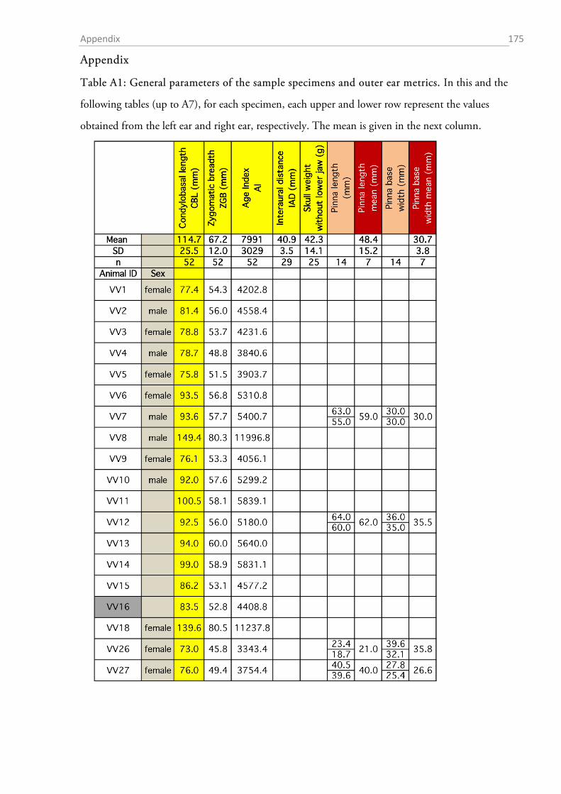
Appendix 175
Appendix
Table A1: General parameters of the sample specimens and outer ear metrics. In this and the
following tables (up to A7), for each specimen, each upper and lower row represent the values
obtained from the left ear and right ear, respectively. The mean is given in the next column.
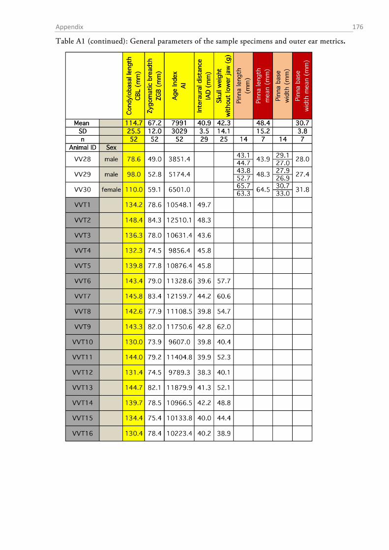
Appendix 176
Table A1 (continued): General parameters of the sample specimens and outer ear metrics.
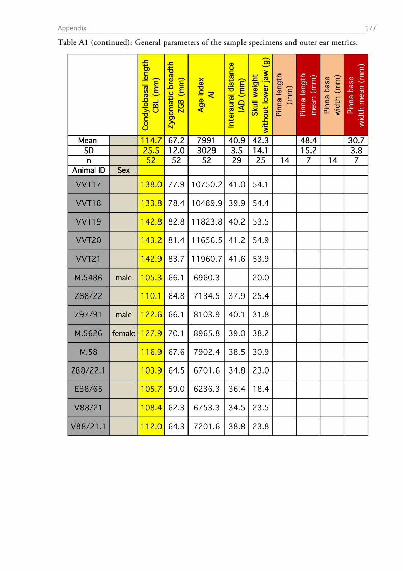
Appendix 177
Table A1 (continued): General parameters of the sample specimens and outer ear metrics.
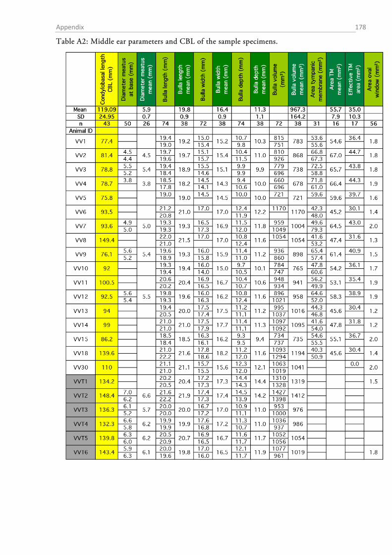
Appendix 178
Table A2: Middle ear parameters and CBL of the sample specimens.
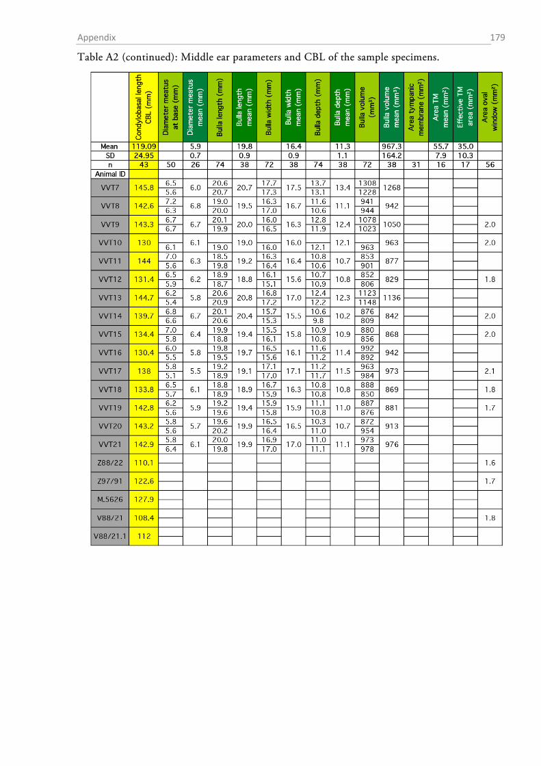
Appendix 179
Table A2 (continued): Middle ear parameters and CBL of the sample specimens.
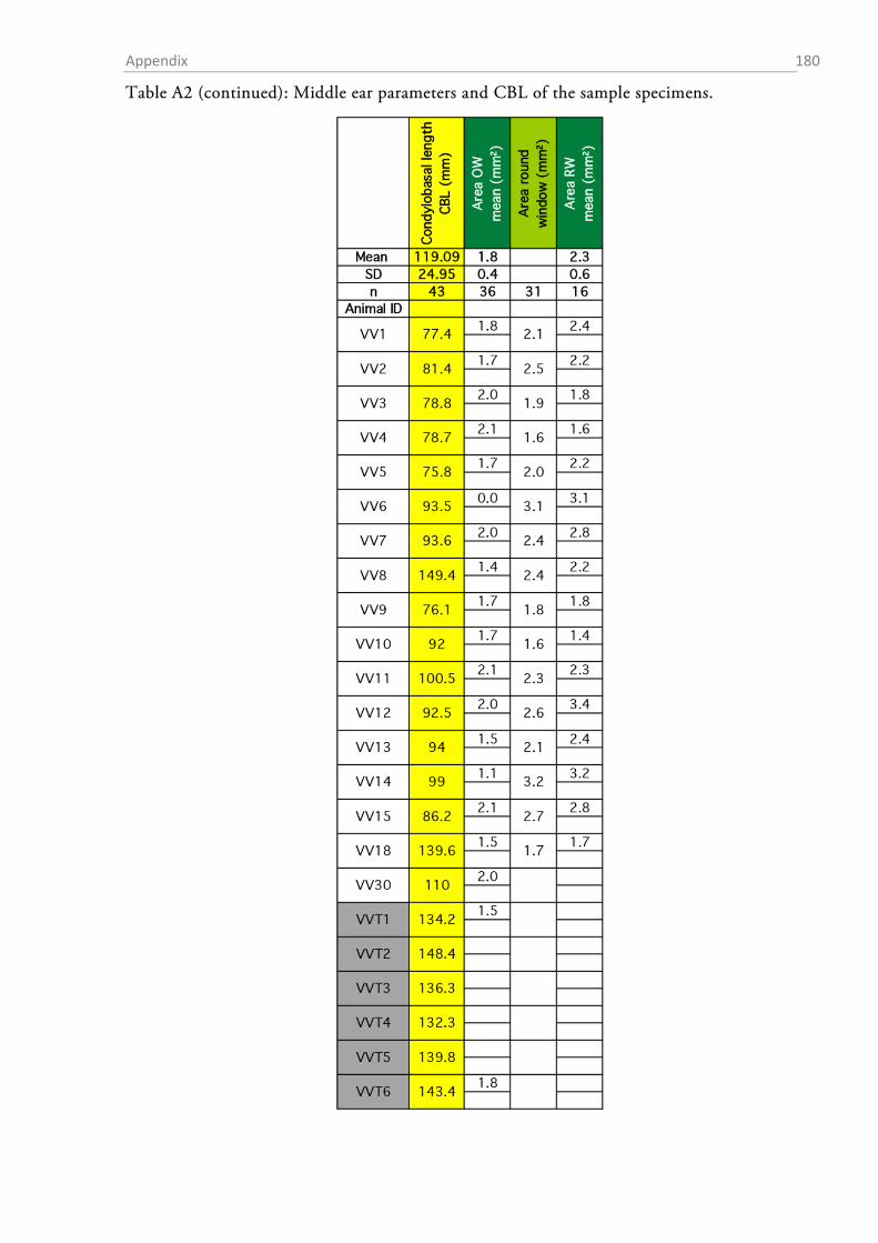
Appendix 180
Table A2 (continued): Middle ear parameters and CBL of the sample specimens.
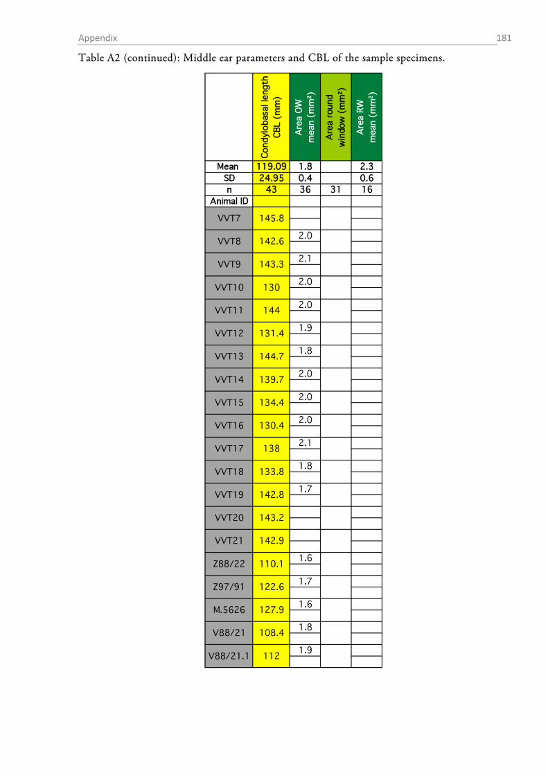
Appendix 181
Table A2 (continued): Middle ear parameters and CBL of the sample specimens.
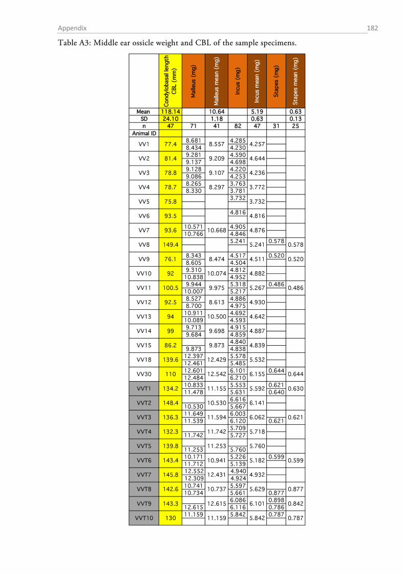
Appendix 182
Table A3: Middle ear ossicle weight and CBL of the sample specimens.
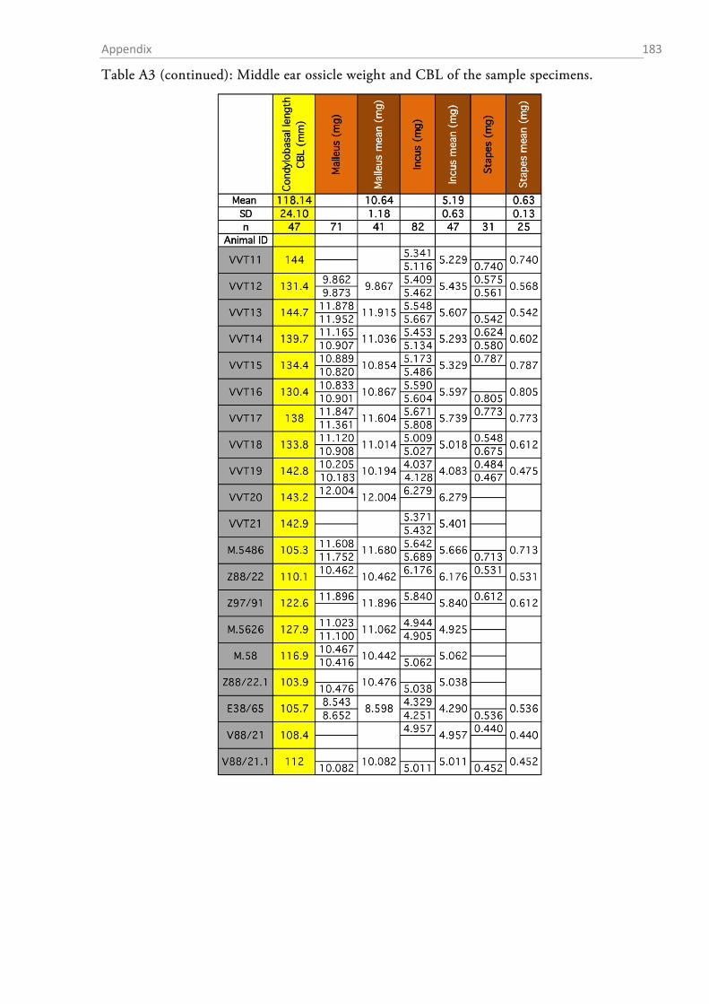
Appendix 183
Table A3 (continued): Middle ear ossicle weight and CBL of the sample specimens.
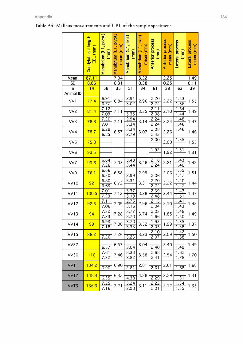
Appendix 184
Table A4: Malleus measurements and CBL of the sample specimens.
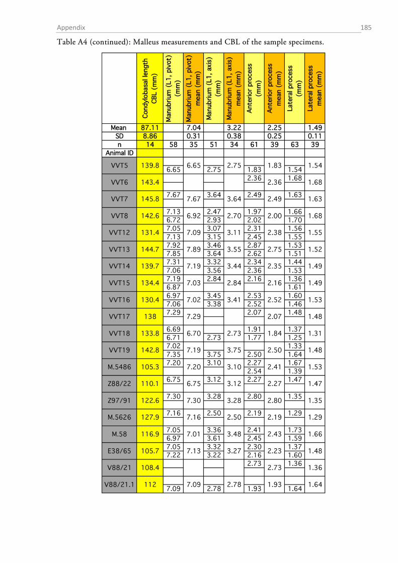
Appendix 185
Table A4 (continued): Malleus measurements and CBL of the sample specimens.
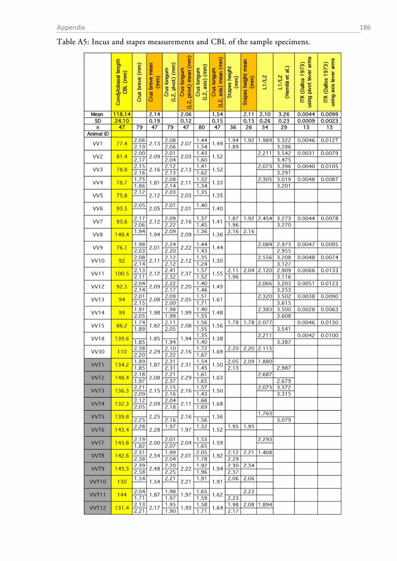
Appendix 186
Table A5: Incus and stapes measurements and CBL of the sample specimens.
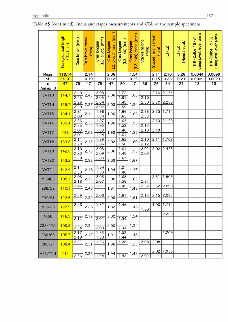
Appendix 187
Table A5 (continued): Incus and stapes measurements and CBL of the sample specimens.
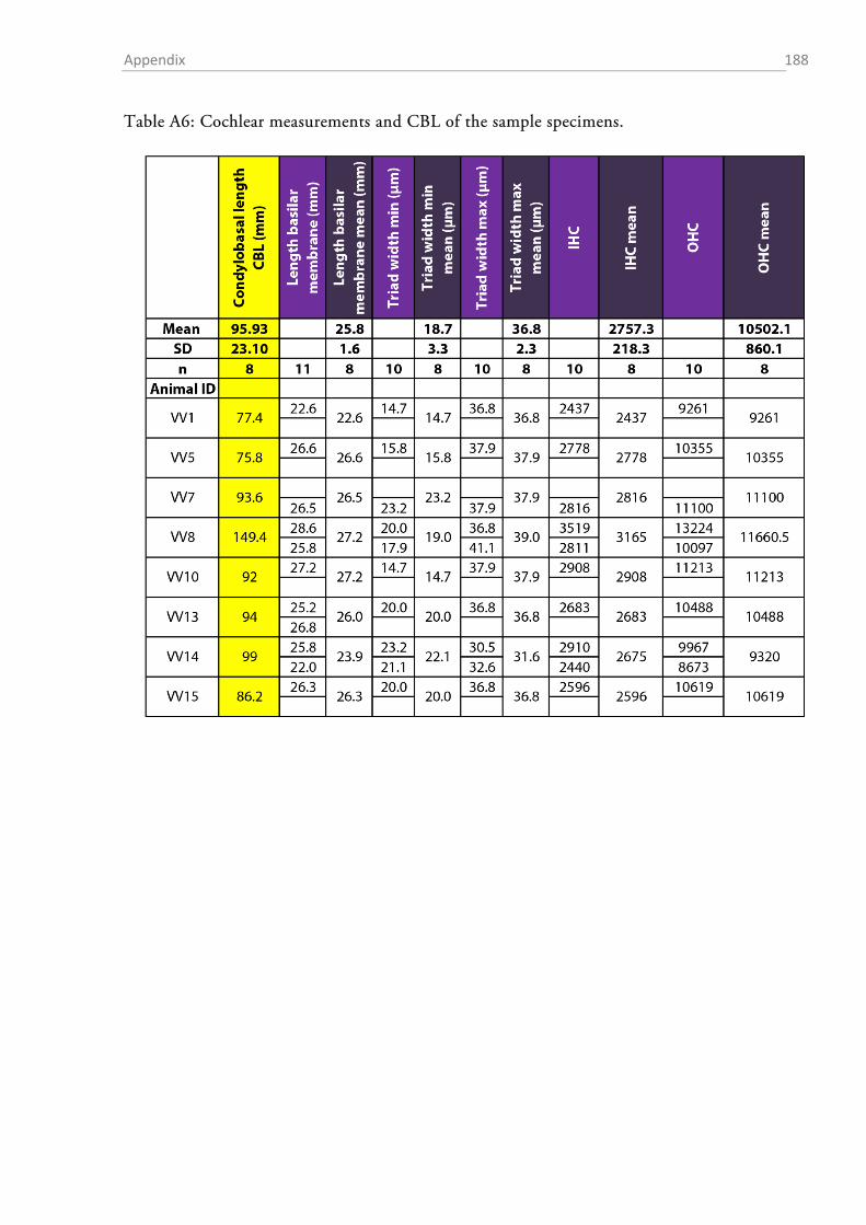
Appendix 188
Table A6: Cochlear measurements and CBL of the sample specimens.
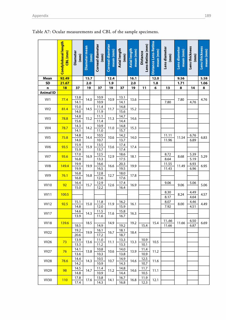
Appendix 189
Table A7: Ocular measurements and CBL of the sample specimens.
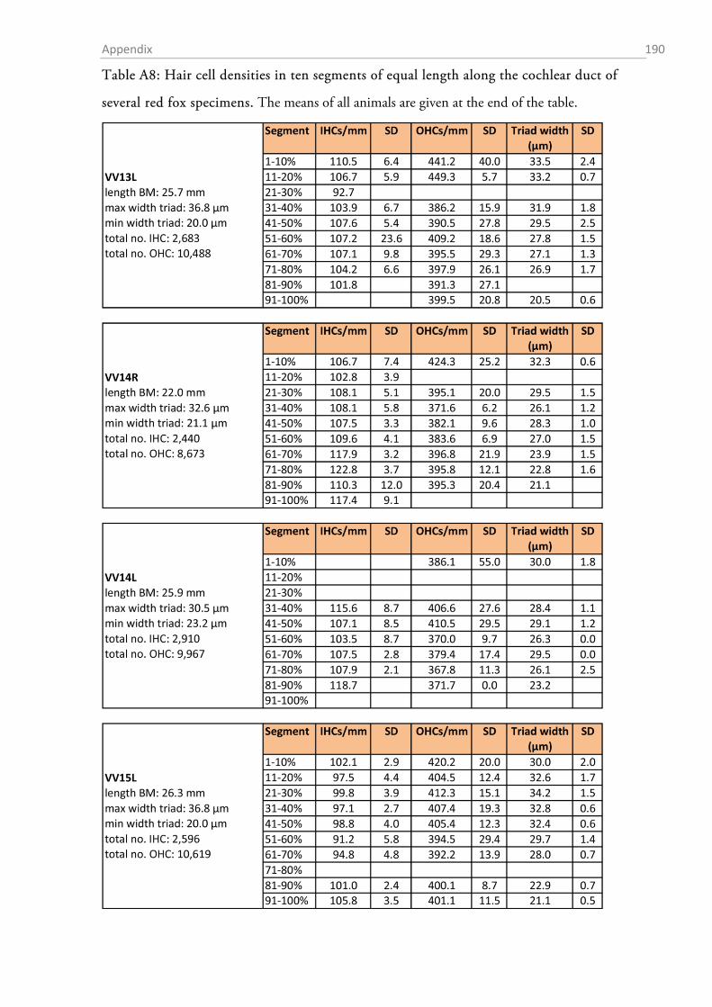
Appendix 190
Table A8: Hair cell densities in ten segments of equal length along the cochlear duct of
several red fox specimens. The means of all animals are given at the end of the table.
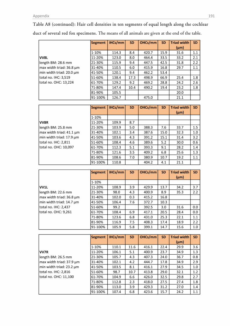
Appendix 191
Table A8 (continued): Hair cell densities in ten segments of equal length along the cochlear
duct of several red fox specimens. The means of all animals are given at the end of the table.
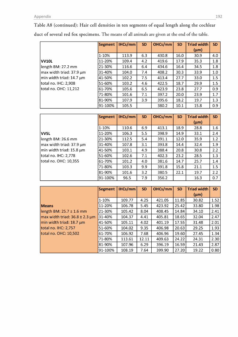
Appendix 192
Table A8 (continued): Hair cell densities in ten segments of equal length along the cochlear
duct of several red fox specimens. The means of all animals are given at the end of the table.
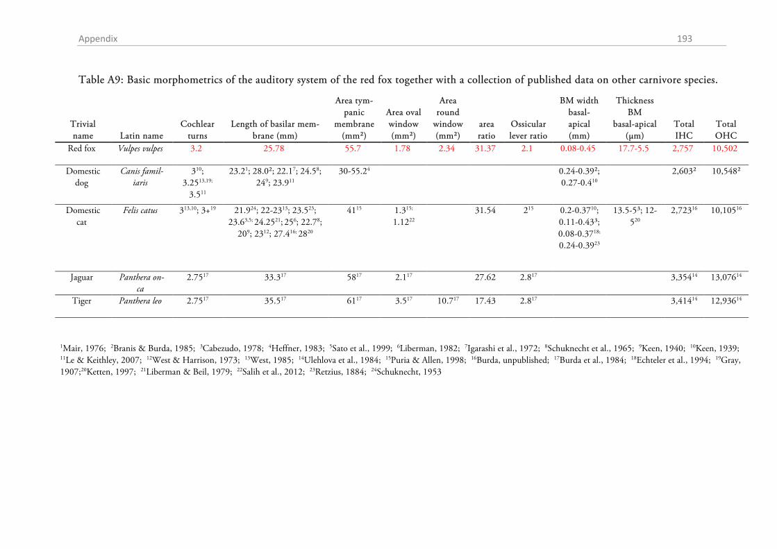
Appendix 193
Table A9: Basic morphometrics of the auditory system of the red fox together with a collection of published data on other carnivore species.
Trivial name Latin name
Cochlear turns
Length of basilar mem-brane (mm)
Area tym-panic
membrane (mm²)
Area oval window (mm²)
Area round
window (mm²)
area ratio
Ossicular lever ratio
BM width basal-apical (mm)
Thickness BM
basal-apical (µm)
Total IHC
Total OHC
Red fox0 Vulpes vulpes0 3.20 25.780 55.70 1.780 2.340 31.370 2.10 0.08-0.450 17.7-5.50 2,7570 10,5020
Domestic dog0
Canis famil-iaris0
310; 3.2513,19;
3.511
23.21; 28.0²; 22.17; 24.58; 249; 23.911
30-55.24 0.24-0.39²; 0.27-0.410
2,603² 10,548²
Domestic cat0
Felis catus0 313,10; 3+19 21.924; 22-2313; 23.523; 23.63,5; 24.2521; 256; 22.78;
209; 2312; 27.416; 2820
4115 1.315;
1.1222 31.540 215 0.2-0.3710;
0.11-0.43³; 0.08-0.3718; 0.24-0.3923
13.5-5³; 12-520
2,72316 10,10516
Jaguar0 Panthera on-ca0
2.7517 33.317 5817 2.117 27.620 2.817 3,35414 13,07614
Tiger0 Panthera leo0 2.7517 35.517 6117 3.517 10.717 17.430 2.817 3,41414 12,93614
1Mair, 1976; 2Branis & Burda, 1985; 3Cabezudo, 1978; 4Heffner, 1983; 5Sato et al., 1999; 6Liberman, 1982; 7Igarashi et al., 1972; 8Schuknecht et al., 1965; 9Keen, 1940; 10Keen, 1939; 11Le & Keithley, 2007; 12West & Harrison, 1973; 13West, 1985; 14Ulehlova et al., 1984; 15Puria & Allen, 1998; 16Burda, unpublished; 17Burda et al., 1984; 18Echteler et al., 1994; 19Gray, 1907;20Ketten, 1997; 21Liberman & Beil, 1979; 22Salih et al., 2012; 23Retzius, 1884; 24Schuknecht, 1953
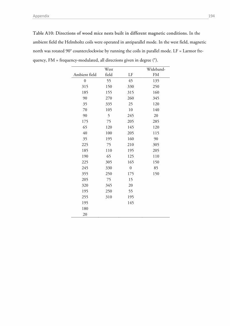
Appendix 194
Table A10: Directions of wood mice nests built in different magnetic conditions. In the
ambient field the Helmholtz coils were operated in antiparallel mode. In the west field, magnetic
north was rotated 90° counterclockwise by running the coils in parallel mode. LF = Larmor fre-
quency, FM = frequency-modulated, all directions given in degree (°).
Ambient field West field LF
Wideband-FM
0 55 45 135 315 150 330 250 185 155 315 160 90 270 260 345 35 335 25 120 70 105 10 140 90 5 245 20 175 75 205 285 65 120 145 120 40 100 205 115 35 195 160 90 225 75 210 305 185 110 195 205 190 65 125 110 225 305 165 150 245 330 0 85 355 250 175 150 205 75 15
320 345 20 195 250 55 255 310 195 195
145
180 20
Eidesstattliche Erklärung 195
Eidesstattliche Erklärung
Erklärung:
Hiermit erkläre ich, gem. § 7 Abs. (2) d) + f) der Promotionsordnung der Fakultät für Biologie
zur Erlangung des Dr. rer. nat., dass ich die vorliegende Dissertation selbständig verfasst und
mich keiner anderen als der angegebenen Hilfsmittel bedient habe und alle wörtlich oder inhalt-
lich übernommenen Stellen als solche gekennzeichnet habe.
Essen, den 25.08.2014 ______________________
(Erich Pascal Malkemper)
Erklärung:
Hiermit erkläre ich, gem. § 7 Abs. (2) e) + g) der Promotionsordnung der Fakultät für Biologie
zur Erlangung des Dr. rer. nat., dass ich keine anderen Promotionen bzw. Promotionsversuche in
der Vergangenheit durchgeführt habe und dass diese Arbeit von keiner anderen Fakul-
tät/Fachbereich abgelehnt worden ist.
Essen, den 25.08.2014 ______________________
(Erich Pascal Malkemper)
Erklärung:
Hiermit erkläre ich, gem. § 6 Abs. (2) g) der Promotionsordnung der Fakultät für Biologie zur
Erlangung der Dr. rer. nat., dass ich das Arbeitsgebiet, dem das Thema „The Sensory Biology of
the Red Fox – Hearing, Vision, Magnetoreception“ zuzuordnen ist, in Forschung und Lehre ver-
trete und den Antrag von Erich Pascal Malkemper befürworte und die Betreuung auch im Falle
eines Weggangs, wenn nicht wichtige Gründe dem entgegenstehen, weiterführen werde.
Essen, den 25.08.2014 ______________________
(Prof. Dr. Hynek Burda)
Abbreviations 196
List of abbreviations
AL axial length ANOVA analysis of variance aq. dest. Aqua destillata BM basilar membrane BMl length of basilar membrane BSA bovine serum albumine CBL condylobasal length cf. confer Cry cryptochrome DAB diaminobenzidin dB decibel dBmax maximum SPL dBmin minimum SPL dBob SPL observing position dpi dots per inch dSPL desired sound pressure level E East EDTA ethylenediaminetetraacetic acid eq. equation FA false alarm FAD flavin adenine dinucleotide FFT fast Fourier transformation FM frequency modulated GCL ganglion cell layer GMF geomagnetic field HE haematoxylin and eosin HT half-turn (cochlea) Hz Hertz IHC inner hair cell ILA incus lever arm (axis) ILD interaural level difference ILP incus lever arm (pivot) INL inner nuclear layer IPL inner plexiform layer IR infrared ISP incus short process ITD interaural time difference IW incus weight LF Larmor frequency LWS (L) long wavelength-sensitive MA magnetic alignment MAP malleus anterior process MF magnetic field MLA malleus lever arm (axis) MLP malleus lateral process MLP malleus lever arm (pivot) MLS medium wavelength-sensitive
mN magnetic North MPM magnetic-particle based mechanism MW malleus weight N North n.d. not determined n.s. not significant NDS normal donkey serum NFR nuclear fast red NGS normal goat serum OHC outer hair cell ONL outer nuclear layer OPL outer plexiform layer OW oval window OWA oval window area P position (along cochlea) Pa Pascal PB phosphate buffer PBS phosphate buffered saline PE pigment epithelium PF pars flaccida PFA paraformaldehyde PL pinna height (length) PND posterior nodal point PrB Prussian blue PT pars tensa PW pinna width RF radiofrequency (magnetic field) RGC retinal ganglion cell RMF retinal magnification factor RPM radical pair mechanism RW round window RWA round window area S South SD single domain SD standard deviation SF single frequency SH stapes height SPL sound pressure level SPM super-paramagnetic SW stapes weight SWS (S) short wavelength-sensitive T Tesla TMA tympanic membrane area tN topographic North W West ZGB zygomatic breadth

CV 197
Der Lebenslauf ist in der Online-Version aus Gründen des Datenschutzes nicht enthalten.

CV 198
Der Lebenslauf ist in der Online-Version aus Gründen des Datenschutzes nicht enthalten.

CV 199
Der Lebenslauf ist in der Online-Version aus Gründen des Datenschutzes nicht enthalten.
CV 200
Der Lebenslauf ist in der Online-Version aus Gründen des Datenschutzes nicht enthalten.
Related Documents


