The Segmentation of Sparse MR Images

The Segmentation of Sparse MR Images

Patrick Craig Marais

A thesis submitted to the Department of Engineering Science� University of Oxford� inpartial ful�lment of the requirements for the degree of Doctor of Philosophy�

Department of Engineering ScienceUniversity of Oxford

Trinity Term��

The Segmentation of Sparse MR Images

Patrick C� Marais

A thesis submitted for the degree of Doctor of Philosophyat the University of Oxford

Robotics Research Group Wolfson CollegeDepartment of Engineering Science Trinity Term ��

Abstract

This thesis develops a methodology for the segmentation of anatomical structures within�sparse MR images� Sparse images were acquired in large numbers prior to the emergenceof highresolution MRI and they form the basis of many long term imaging studies�

The term sparse refers to the fact that the volumetric image has very poor spatial resolution inthe direction perpendicular to the slice plane� This leads to a signi�cant degradation in imagequality and e�ectively destroys the spatial continuity of the imaged object� Consequently�generic segmentation schemes � particularly those based on voxel classi�cation � will yieldpoor results unless they have been augmented in some manner�

Our Segmentation approach is based on a deformable simplex mesh surface� which iterativelyinterpolates extracted boundary point data� Prior information is mobilised at two levels�Boundary points are found using a matching algorithm based on a database of prespeci�edpiecewise constant models� These models represent possible idealised intensity pro�les forthe object boundary� In addition to the boundary model� there is a shape template� Thetemplate is generated from a training set of presegmented structures� which means that onlyshapes similar to those in the training set will be recovered� The segmentation proceedsin two phases� The �rst recovers the normal shape component� determined by the trainingset� whilst the second deforms smoothly from this constrained solution to produce a moreveridical boundary representation�

The segmentation scheme is applied to a number of sparse brain images� Qualitative validation � accomplished by registering the surface extracted from the sparse data to a highresolution scan acquired at the same timepoint � indicates that a good approximation tothe underlying boundary is obtainable from such images�

i

Acknowledgements

This work was supported in part by funds from the Foundation for Research Development FRD� in South Africa� an ORS award UK�� and the European Community BiomorphProject No� �� Additional material resources were supplied by the MRC Schizophrenia Research Unit Radcli�e In�rmary� Oxford�� headed by our principal collaborator� DrTim Crow� MR data was provided by Prof Lynn DeLisi� of the Dept� of Psychiatry� SUNY�Additional data was obtained from the Biomorph data pool� which was sourced by severaldi�erent institutes�

The simplex mesh software around which much of this work built was kindly provided by DrHerve Dellingette of INRIA� SophiaAntipolis� If this software had not existed� my life wouldhave been considerably more complicated� Within Oxford itself� there are many who havein�uenced the �nal form of this work� Dr Jacques Feldmar� now engaged in entrepreneurialpursuits� was a great source of ideas and inspiration� My coworkers have all contributed insome way or another� for which they have my gratitude� In particular� I would like to thankSebastien Gilles for several useful suggestions with regards to boundary matching� Finally� Iextend my sincerest thanks to my supervisors� Mike Brady and Andrew Zisserman� Withouttheir guidance and support� this work would not have been possible�

This thesis is dedicated to those� both past and present� who have inspired me to pursue mydreams� My gratitude to you is eternal�

ii

Contents

� Introduction �

�� Background � � � � � � � � � � � � � � � � � � � � � � � � � � � � � � � � � � � � � �

�� The Structure of the Brain � � � � � � � � � � � � � � � � � � � � � � � � �

�� Brain Asymmetry and Schizophrenia � � � � � � � � � � � � � � � � � � � �

�� Clinical Studies of Brain Asymmetry � � � � � � � � � � � � � � � � � � � �

�� A Framework for the Segmentation of Sparse MRI � � � � � � � � � � � � � � � �

�� Thesis Structure � � � � � � � � � � � � � � � � � � � � � � � � � � � � � � � � � � ��

� Preliminaries ��

�� Magnetic Resonance Imaging � � � � � � � � � � � � � � � � � � � � � � � � � � � ��

�� Nuclear Magnetic Resonance � � � � � � � � � � � � � � � � � � � � � � � ��

�� Image Formation � � � � � � � � � � � � � � � � � � � � � � � � � � � � � � ��

�� MRI Slice Resolution � � � � � � � � � � � � � � � � � � � � � � � � � � � � ��

�� MRI Contrast � � � � � � � � � � � � � � � � � � � � � � � � � � � � � � � � ��

�� MRI Artifacts � � � � � � � � � � � � � � � � � � � � � � � � � � � � � � � � ��

�� Characterisation of Sparse MRI Data � � � � � � � � � � � � � � � � � � � � � � � ��

�� Sparse MR Images � � � � � � � � � � � � � � � � � � � � � � � � � � � � � ��

�� Sparse MR Image Database � � � � � � � � � � � � � � � � � � � � � � � � ��

�� Segmentation Issues � � � � � � � � � � � � � � � � � � � � � � � � � � � � ��

�� Overview of Segmentation Methods � � � � � � � � � � � � � � � � � � � � � � � � ��

�� VoxelClassi�cation Schemes � � � � � � � � � � � � � � � � � � � � � � � ��

�� Constraining Shape � � � � � � � � � � � � � � � � � � � � � � � � � � � � ��

�� Conclusion � � � � � � � � � � � � � � � � � � � � � � � � � � � � � � � � � � � � � ��

iii

� Snakes ��

�� The Snake Framework � � � � � � � � � � � � � � � � � � � � � � � � � � � � � � � ��

�� Modi�ed Framework � � � � � � � � � � � � � � � � � � � � � � � � � � � � ��

�� Segmentation � � � � � � � � � � � � � � � � � � � � � � � � � � � � � � � � � � � � ��

�� Initialisation Issues � � � � � � � � � � � � � � � � � � � � � � � � � � � � � ��

�� D Feature Detection � � � � � � � � � � � � � � � � � � � � � � � � � � � ��

�� Position Update � � � � � � � � � � � � � � � � � � � � � � � � � � � � � � ��

�� Correspondence Over Slices � � � � � � � � � � � � � � � � � � � � � � � � ��

�� Results � � � � � � � � � � � � � � � � � � � � � � � � � � � � � � � � � � � ��

�� Surface Construction and MidSaggital Plane Estimation � � � � � � � � � � � ��

�� MSP Estimation � � � � � � � � � � � � � � � � � � � � � � � � � � � � � � ��

�� Surface Construction � � � � � � � � � � � � � � � � � � � � � � � � � � � � ��

�� Discussion � � � � � � � � � � � � � � � � � � � � � � � � � � � � � � � � � � � � � � ��

�� Edge Model Robustness � � � � � � � � � � � � � � � � � � � � � � � � � � ��

�� Coping with Topology and Geometry � � � � � � � � � � � � � � � � � � ��

�� Conclusion � � � � � � � � � � � � � � � � � � � � � � � � � � � � � � � � � � � � � ��

� Constructing a Shape Template ��

�� The Simplex Mesh � � � � � � � � � � � � � � � � � � � � � � � � � � � � � � � � � ��

�� Learning Shape Variation � � � � � � � � � � � � � � � � � � � � � � � � � � � � � ��

�� Principal Components Analysis � � � � � � � � � � � � � � � � � � � � � � ��

�� The Point Distribution Model � � � � � � � � � � � � � � � � � � � � � � � ��

�� Generation of the Mesh Training Set � � � � � � � � � � � � � � � � � � � � � � � ��

�� Establishing Point Correspondences � � � � � � � � � � � � � � � � � � � � � � � ��

�� Correspondent Extraction � � � � � � � � � � � � � � � � � � � � � � � � � ��

�� Dealing with Correspondence Errors � � � � � � � � � � � � � � � � � � � ��

�� Analysis of Registration Schemes � � � � � � � � � � � � � � � � � � � � � � � � � ��

�� Type I� Bounding Box Registration � � � � � � � � � � � � � � � � � � � � ��

�� Type II� ICP Registration � � � � � � � � � � � � � � � � � � � � � � � � � ��

�� Results � � � � � � � � � � � � � � � � � � � � � � � � � � � � � � � � � � � � � � � � ��

�� Vertex Redistribution � � � � � � � � � � � � � � � � � � � � � � � � � � � ��

�� Resampling Errors � � � � � � � � � � � � � � � � � � � � � � � � � � � � � ��

�� Projection Error � � � � � � � � � � � � � � � � � � � � � � � � � � � � � � ��

�� Qualitative Assessment of Correspondences � � � � � � � � � � � � � � � ��

iv

�� Discussion � � � � � � � � � � � � � � � � � � � � � � � � � � � � � � � � � � � � � � ��

�� Conclusion � � � � � � � � � � � � � � � � � � � � � � � � � � � � � � � � � � � � � ��

� Boundary Detection ��

�� The Brain Surface Boundary � � � � � � � � � � � � � � � � � � � � � � � � � � � ��

�� The Boundary Model Framework � � � � � � � � � � � � � � � � � � � � � � � � � ��

�� Model Input Data � � � � � � � � � � � � � � � � � � � � � � � � � � � � � ��

�� The Models � � � � � � � � � � � � � � � � � � � � � � � � � � � � � � � � � ��

�� Edge Heuristics � � � � � � � � � � � � � � � � � � � � � � � � � � � � � � � � � � � ��

�� Node Modelling � � � � � � � � � � � � � � � � � � � � � � � � � � � � � � � � � � � ��

�� Specifying a model � � � � � � � � � � � � � � � � � � � � � � � � � � � � � � � � � ��

�� Model Construction and Representation � � � � � � � � � � � � � � � � � ��

�� Matching the Model to Data � � � � � � � � � � � � � � � � � � � � � � � ��

�� Model Decomposition � � � � � � � � � � � � � � � � � � � � � � � � � � � ��

�� Coarse Matching � � � � � � � � � � � � � � � � � � � � � � � � � � � � � � ��

�� Local Matching � � � � � � � � � � � � � � � � � � � � � � � � � � � � � � � ��

�� Model Constraints � � � � � � � � � � � � � � � � � � � � � � � � � � � � � ��

�� Matching for Multiple Boundary Classes � � � � � � � � � � � � � � � � � ��

�� Discretisation Issues � � � � � � � � � � � � � � � � � � � � � � � � � � � � ��

�� Dealing with Cortical Folding � � � � � � � � � � � � � � � � � � � � � � � � � � � ��

�� Boundary Detection Results � � � � � � � � � � � � � � � � � � � � � � � � � � � � ��

�� Model Setup and Parameters � � � � � � � � � � � � � � � � � � � � � � � ��

�� Results � � � � � � � � � � � � � � � � � � � � � � � � � � � � � � � � � � � ��

�� Discussion � � � � � � � � � � � � � � � � � � � � � � � � � � � � � � � � � � � � � � ��

�� Conclusion � � � � � � � � � � � � � � � � � � � � � � � � � � � � � � � � � � � � � ��

� Modelling the Partial Volume Eect ��

�� Related Work � � � � � � � � � � � � � � � � � � � � � � � � � � � � � � � � � � � � ��

�� The MR Imaging model � � � � � � � � � � � � � � � � � � � � � � � � � � � � � � ��

�� The Prediction Scheme � � � � � � � � � � � � � � � � � � � � � � � � � � � � � � � ��

�� The Boundary Detection Strategy � � � � � � � � � � � � � � � � � � � � � � � � ��

�� Experiments on Synthetic Data � � � � � � � � � � � � � � � � � � � � � � � � � � ��

�� Test Data � � � � � � � � � � � � � � � � � � � � � � � � � � � � � � � � � � ��

�� Quantifying Edge Estimation Errors � � � � � � � � � � � � � � � � � � � ��

v

�� Prediction Using Matched Models � � � � � � � � � � � � � � � � � � � � ��

�� Discussion � � � � � � � � � � � � � � � � � � � � � � � � � � � � � � � � � � � � � � ��

�� Conclusion � � � � � � � � � � � � � � � � � � � � � � � � � � � � � � � � � � � � � ��

� Surface�based Segmentation ��

�� Utilising the Shape Constraint � � � � � � � � � � � � � � � � � � � � � � � � � � ��

�� The Segmentation Framework � � � � � � � � � � � � � � � � � � � � � � � � � � � ��

�� Template Initialisation � � � � � � � � � � � � � � � � � � � � � � � � � � � � � � � ��

�� Computing the Template Bounding Box � � � � � � � � � � � � � � � � � ��

�� Computing the Shape Instance Bounding Box � � � � � � � � � � � � � � ��

�� Initialisation Examples � � � � � � � � � � � � � � � � � � � � � � � � � � � ��

�� Computing the Surface Update � � � � � � � � � � � � � � � � � � � � � � � � � � ��

�� The Implications of Truncation and Sparsity � � � � � � � � � � � � � � ��

�� Computing the Closest Point Deformation � � � � � � � � � � � � � � � � ��

�� Stage I� ASM Segmentation � � � � � � � � � � � � � � � � � � � � � � � � ��

�� Stage II� Simplex Segmentation � � � � � � � � � � � � � � � � � � � � � � ��

�� Results � � � � � � � � � � � � � � � � � � � � � � � � � � � � � � � � � � � � � � � � ��

�� The Template � � � � � � � � � � � � � � � � � � � � � � � � � � � � � � � � ��

�� Test Database � � � � � � � � � � � � � � � � � � � � � � � � � � � � � � � ��

�� Parameters � � � � � � � � � � � � � � � � � � � � � � � � � � � � � � � � � ��

�� Sparse Segmentation � � � � � � � � � � � � � � � � � � � � � � � � � � � � ��

�� Discussion � � � � � � � � � � � � � � � � � � � � � � � � � � � � � � � � � � � � � � ��

�� Conclusion � � � � � � � � � � � � � � � � � � � � � � � � � � � � � � � � � � � � � ��

� Conclusion ��

�� Future Work � � � � � � � � � � � � � � � � � � � � � � � � � � � � � � � � � � � � ��

�� The Shape Template � � � � � � � � � � � � � � � � � � � � � � � � � � � � ��

�� The Boundary Model � � � � � � � � � � � � � � � � � � � � � � � � � � � ��

�� PVE Prediction � � � � � � � � � � � � � � � � � � � � � � � � � � � � � � � ��

�� Segmenting Other Structures � � � � � � � � � � � � � � � � � � � � � � � ��

�� Asymmetry�Shape Analysis � � � � � � � � � � � � � � � � � � � � � � � � ��

APPENDICES ��

vi

A B�Spline snakes ��

A�� De�nition � � � � � � � � � � � � � � � � � � � � � � � � � � � � � � � � � � � � � � ��

A�� Area measurements � � � � � � � � � � � � � � � � � � � � � � � � � � � � � � � � � ��

B The Simplex Mesh Formalism ��

B�� Geometric Properties � � � � � � � � � � � � � � � � � � � � � � � � � � � � � � � � ��

B�� Metric Parameters � � � � � � � � � � � � � � � � � � � � � � � � � � � � � � � � � ��

B�� The Simplex Mesh and Segmentation � � � � � � � � � � � � � � � � � � � � � � � ��

B�� Internal Forces � � � � � � � � � � � � � � � � � � � � � � � � � � � � � � � ��

B�� External Forces � � � � � � � � � � � � � � � � � � � � � � � � � � � � � � � ��

C Mesh Measures ��

C�� Surface Area � � � � � � � � � � � � � � � � � � � � � � � � � � � � � � � � � � � � ��

C�� Volume � � � � � � � � � � � � � � � � � � � � � � � � � � � � � � � � � � � � � � � ��

C�� Transforming the PCA Eigensystem � � � � � � � � � � � � � � � � � � � � � � � ��

D Mahalanobis PCA criterion ��

E Cosine Foreshortening for Curved Surfaces ��

E�� An Example � � � � � � � � � � � � � � � � � � � � � � � � � � � � � � � � � � � � � ��

F T� Boundary Model Database ��

Bibliography ��

vii

List of Figures

�� Two Views of the Brain � � � � � � � � � � � � � � � � � � � � � � � � � � � � � � �

�� The Ventricular System � � � � � � � � � � � � � � � � � � � � � � � � � � � � � � �

�� Laterality Measures � � � � � � � � � � � � � � � � � � � � � � � � � � � � � � � � �

�� The Laterality Index � � � � � � � � � � � � � � � � � � � � � � � � � � � � � � � � �

�� Simplex Mesh ventricular� Model � � � � � � � � � � � � � � � � � � � � � � � � �

�� Model Constraints � � � � � � � � � � � � � � � � � � � � � � � � � � � � � � � � � �

�� Inplane boundary detection � � � � � � � � � � � � � � � � � � � � � � � � � � � � �

�� E�ect of a Magnetic Field � � � � � � � � � � � � � � � � � � � � � � � � � � � � � ��

�� RF Resonance and Relaxation � � � � � � � � � � � � � � � � � � � � � � � � � � � ��

�� KSpace � � � � � � � � � � � � � � � � � � � � � � � � � � � � � � � � � � � � � � � ��

�� An MRI Image � � � � � � � � � � � � � � � � � � � � � � � � � � � � � � � � � � � ��

�� Bias Field � � � � � � � � � � � � � � � � � � � � � � � � � � � � � � � � � � � � � � ��

�� Imaging Artifacts � � � � � � � � � � � � � � � � � � � � � � � � � � � � � � � � � � ��

�� Partial Volume E�ects � � � � � � � � � � � � � � � � � � � � � � � � � � � � � � � ��

�� Data Truncation � � � � � � � � � � � � � � � � � � � � � � � � � � � � � � � � � � ��

�� Voxel Segmentation � � � � � � � � � � � � � � � � � � � � � � � � � � � � � � � � � ��

�� Snake Feature Search � � � � � � � � � � � � � � � � � � � � � � � � � � � � � � � � ��

�� Snake Segmentation � � � � � � � � � � � � � � � � � � � � � � � � � � � � � � � � ��

�� Predicted Quantities � � � � � � � � � � � � � � � � � � � � � � � � � � � � � � � � ��

�� Motion Prediction � � � � � � � � � � � � � � � � � � � � � � � � � � � � � � � � � ��

�� MidSaggital Line CrossSections � � � � � � � � � � � � � � � � � � � � � � � � � ��

�� MidSaggital Estimation � � � � � � � � � � � � � � � � � � � � � � � � � � � � � � ��

�� Steps in Surface Construction � � � � � � � � � � � � � � � � � � � � � � � � � � � ��

�� Principal Components � � � � � � � � � � � � � � � � � � � � � � � � � � � � � � � ��

�� Snake Segmentation � � � � � � � � � � � � � � � � � � � � � � � � � � � � � � � � ��

viii

�� Mesh Surface Representation � � � � � � � � � � � � � � � � � � � � � � � � � � � ��

�� Correspondent Selection � � � � � � � � � � � � � � � � � � � � � � � � � � � � � � ��

�� Correspondent Inversions � � � � � � � � � � � � � � � � � � � � � � � � � � � � � ��

�� Example of Vertex Redistribution for a Curve � � � � � � � � � � � � � � � � � � ��

�� Comparison of PCA Methods � � � � � � � � � � � � � � � � � � � � � � � � � � � ��

�� Normal Selection Vertex Redistribution � � � � � � � � � � � � � � � � � � � � � ��

�� Closest Point Vertex Redistribution � � � � � � � � � � � � � � � � � � � � � � � � ��

�� Global Registration � � � � � � � � � � � � � � � � � � � � � � � � � � � � � � � � � ��

�� PDM Deformation Modes � � � � � � � � � � � � � � � � � � � � � � � � � � � � � ��

�� Projection Errors � � � � � � � � � � � � � � � � � � � � � � � � � � � � � � � � � � ��

�� Randomly Selected Correspondents Bottom View� � � � � � � � � � � � � � � � ��

�� Selected Correspondents Side View� � � � � � � � � � � � � � � � � � � � � � � � ��

�� Correspondent Point Clustering � � � � � � � � � � � � � � � � � � � � � � � � � � ��

�� Correspondent Selection � � � � � � � � � � � � � � � � � � � � � � � � � � � � � � ��

�� Spline Deformation � � � � � � � � � � � � � � � � � � � � � � � � � � � � � � � � � ��

�� Cerebral Boundary Structure � � � � � � � � � � � � � � � � � � � � � � � � � � � ��

�� Cortical Folding � � � � � � � � � � � � � � � � � � � � � � � � � � � � � � � � � � � ��

�� Edge Heuristics � � � � � � � � � � � � � � � � � � � � � � � � � � � � � � � � � � � ��

�� Matching Under the Mahalanobis Criterion � � � � � � � � � � � � � � � � � � � ��

�� Pro�le PCA � � � � � � � � � � � � � � � � � � � � � � � � � � � � � � � � � � � � � ��

�� Poor Boundary Model � � � � � � � � � � � � � � � � � � � � � � � � � � � � � � � ��

�� Matching with a Dynamic Boundary Model � � � � � � � � � � � � � � � � � � � ��

�� Simple Translation � � � � � � � � � � � � � � � � � � � � � � � � � � � � � � � � � ��

�� Model Elements � � � � � � � � � � � � � � � � � � � � � � � � � � � � � � � � � � � ��

�� Coarse to Fine Matching � � � � � � � � � � � � � � � � � � � � � � � � � � � � � � ��

�� Model Decomposition � � � � � � � � � � � � � � � � � � � � � � � � � � � � � � � ��

�� Coarse Matching � � � � � � � � � � � � � � � � � � � � � � � � � � � � � � � � � � ��

�� Local Matching � � � � � � � � � � � � � � � � � � � � � � � � � � � � � � � � � � � ��

�� Vertical Fitting � � � � � � � � � � � � � � � � � � � � � � � � � � � � � � � � � � � ��

�� Order of Local Matching � � � � � � � � � � � � � � � � � � � � � � � � � � � � � � ��

�� Model Re�nement � � � � � � � � � � � � � � � � � � � � � � � � � � � � � � � � � ��

�� Validation Pro�les � � � � � � � � � � � � � � � � � � � � � � � � � � � � � � � � � ��

�� Edge Detection Example One � � � � � � � � � � � � � � � � � � � � � � � � � � ��

ix

�� Edge Detection Example Two � � � � � � � � � � � � � � � � � � � � � � � � � � ��

�� Examples of Matched Models � � � � � � � � � � � � � � � � � � � � � � � � � � � ��

�� The Need for Coarse Models � � � � � � � � � � � � � � � � � � � � � � � � � � � � ��

�� Voxel Partial Volume � � � � � � � � � � � � � � � � � � � � � � � � � � � � � � � � ��

�� Prediction of Local Intensities � � � � � � � � � � � � � � � � � � � � � � � � � � � ��

�� Pro�le Prediction and Matching � � � � � � � � � � � � � � � � � � � � � � � � � ��

�� Synthetic Volumetric Data � � � � � � � � � � � � � � � � � � � � � � � � � � � � � ��

�� Partial Volumes and Edge Location � � � � � � � � � � � � � � � � � � � � � � � � ��

�� Matching in the Presence of Noise � � � � � � � � � � � � � � � � � � � � � � � � ��

�� Estimates with Model Noise ��mm sphere� � � � � � � � � � � � � � � � � � � ��

�� Estimates with Model Noise ��mm sphere� � � � � � � � � � � � � � � � � � � ��

�� Image and Model Noise ��mm sphere� � � � � � � � � � � � � � � � � � � � � � ��

�� Prediction in Real Data Using a Single Boundary Model � � � � � � � � � � � � ��

�� Prediction Using A Good Model � � � � � � � � � � � � � � � � � � � � � � � � � ��

�� Prediction Using Coarse or Incomplete Models � � � � � � � � � � � � � � � � � ��

�� D Active Shape Model � � � � � � � � � � � � � � � � � � � � � � � � � � � � � � ��

�� Template Initialisation � � � � � � � � � � � � � � � � � � � � � � � � � � � � � � � ��

�� Computing the Initialisation � � � � � � � � � � � � � � � � � � � � � � � � � � � � ��

�� Robust Plane Estimation � � � � � � � � � � � � � � � � � � � � � � � � � � � � � ��

�� Poor Boundary Discrimination � � � � � � � � � � � � � � � � � � � � � � � � � � ��

�� A�ne ICP� Segmentation � � � � � � � � � � � � � � � � � � � � � � � � � � � � � ��

�� Closest Point Deformation � � � � � � � � � � � � � � � � � � � � � � � � � � � � � ��

�� Deformation Cusp � � � � � � � � � � � � � � � � � � � � � � � � � � � � � � � � � ��

�� ASM Constrained Segmentation � � � � � � � � � � � � � � � � � � � � � � � � � ��

�� External Force Decay � � � � � � � � � � � � � � � � � � � � � � � � � � � � � � � ��

�� Simplex Template Segmentation � � � � � � � � � � � � � � � � � � � � � � � � � ��

�� Cerebral Contours � Example � � � � � � � � � � � � � � � � � � � � � � � � � � ��

�� Full Cerebral Surface � � � � � � � � � � � � � � � � � � � � � � � � � � � � � � � � ��

�� Mesh Contours in Sparse Data � Example � � � � � � � � � � � � � � � � � � � ��

�� Mesh Contours in Dense Data � Example � � � � � � � � � � � � � � � � � � � ��


�� Mesh Contours in Dense Data � Example � � � � � � � � � � � � � � � � � � � ��

x


�� Sulcal Mismatch � � � � � � � � � � � � � � � � � � � � � � � � � � � � � � � � � � ��

�� Merged Boundaries � � � � � � � � � � � � � � � � � � � � � � � � � � � � � � � � � ��

�� Symmetry Map � � � � � � � � � � � � � � � � � � � � � � � � � � � � � � � � � � � ��

A�� Cubic Bspline � � � � � � � � � � � � � � � � � � � � � � � � � � � � � � � � � � � ��

B�� Simplex Mesh Triangulation � � � � � � � � � � � � � � � � � � � � � � � � � � � � ��

B�� Simplex Angle � � � � � � � � � � � � � � � � � � � � � � � � � � � � � � � � � � � ��

B�� Metric Parameters � � � � � � � � � � � � � � � � � � � � � � � � � � � � � � � � � ��

B�� Sti�ness Function � � � � � � � � � � � � � � � � � � � � � � � � � � � � � � � � � � ��

E�� Cosine Foreshortening � � � � � � � � � � � � � � � � � � � � � � � � � � � � � � � ��

E�� Cosine Foreshortening on the Sphere � � � � � � � � � � � � � � � � � � � � � � � ��

E�� Foreshortening Example � � � � � � � � � � � � � � � � � � � � � � � � � � � � � � ��

F�� Model Database � � � � � � � � � � � � � � � � � � � � � � � � � � � � � � � � � � ��

xi

List of Tables

�� MRI ContrastWeighting Schemes � � � � � � � � � � � � � � � � � � � � � � � � ��

F�� Model Parameters � � � � � � � � � � � � � � � � � � � � � � � � � � � � � � � � � ��

xii

Chapter �

Introduction

The introduction of magnetic resonance imaging MRI� marked a signi�cant milestone in

the development of diagnostic radiology� The excellent soft tissue discrimination a�orded by

MRI allows for the detection of subtle pathologies which are often invisible or poorly resolved

under other imaging modalities� It is also noninvasive� and has no demonstrable side e�ects�

These characteristics have ensured that MRI has rapidly emerged as the modality of choice

for the investigation of a range of neurological disorders�

An analysis of brain structure necessitates some sort of segmentation of the data� For our

purposes� segmentation refers to the extraction and description of speci�ed� anatomical

structures within the imaged volume� Unfortunately the tremendous variability of anatom

ical structures� coupled with poor resolution and inescapable imaging artifacts� renders this

task extremely di�cult in all but the simplest of cases� These limitations are of particu

lar importance to us� since our MR data is sparse� In this context� the term sparse refers

to the fact that the spatial resolution of the volumetric image is much coarser along one

axis than the other two� A detailed description of the image sequences we employed will

be given in Section �� Although current MR technology allows for the acquisition of high

resolution image sequences� we cannot simply disregard existing sparse data sequences� Such

data sets constitute an important part of valuable long term studies� spanning the last ��

years� and reliable techniques must be developed to assist radiologists in processing them�

The investigation of brain asymmetry in schizophrenics is one such area� and served as the

primary motivation for this work� Although this thesis does not address the issue of brain

asymmetry directly though a clinical study�� the issues involved in brain segmentation are

well illustrated by work in this area� and we shall therefore refer extensively to the relevant

literature�

The objective of this work is the development of robust algorithms to segment anatomical

structures from sparse MRI sequences� We seek a methodology which will allow us to in

�If no contrast agents are used�

�

corporate our knowledge of the domain� the successful exploitation of such information may

well mean the di�erence between success or failure�

�� Background

The brain is a complex structure with very speci�c segmentation requirements� The tech

niques developed here will be tested on sparse brain MR images� since the segmentation of

such data provides a challenging application and is a precursor to any subsequent analysis

of brain asymmetry� To help appreciate the issues involved� we provide a brief overview of

brain anatomy and review a number of segmentation techniques used by other researchers in

this area�

�� The Structure of the Brain

The Brain is composed of white and grey �cortical� matter � the latter consists of neurons� the

fundamental processing units of the brain� whilst the former provides the connections which

link these cells together� Grey matter envelopes white and is arranged so as to maximise

its surface area in the cramped con�nes of the skull� The resulting cortical folding� which is

characteristic of the largest uppermost� part of the brain� the cerebrum� gives rise to sulci

and gyri� Sulci are winding �ssures which work their way across the cerebral surface� These

sulci� in turn� delineate the gyri � ridges of cortical matter which give the cerebrum its

characteristic lumpy look � Figure �� The cerebellum� which is attached to the underside

of the cerebrum� is a less sophisticated structure� being both smaller and possessing a less

convoluted surface geometry� Its primary function is the regulation and maintenance of

autonomous processes � those which are considered �instinctive�

The cerebrum is decomposed into a series of lobes � frontal� temporal� parietal and occipital

� Figure �� Their delineation is somewhat imprecise� since the boundaries are assumed to

lie along certain major sulci and these are frequently displaced across patients� The temporal

lobe is bounded by the sylvian �ssure� a prominent sulcus which is often used to de�ne

anatomically stable landmarks�

There is a natural bilaterality to the brain� which is most clearly demonstrated by the bifur

cation of the cerebrum into the left and right cerebral hemispheres� The interhemispheric

�ssure� or mid�saggital plane �MSP�� provides an approximate plane of symmetry� but one

which is only de�ned over part of the brain� the hemispheres fuse together in an interconnect

known as the corpus callosum� The cerebellum is similarly divided� The interior of the brain

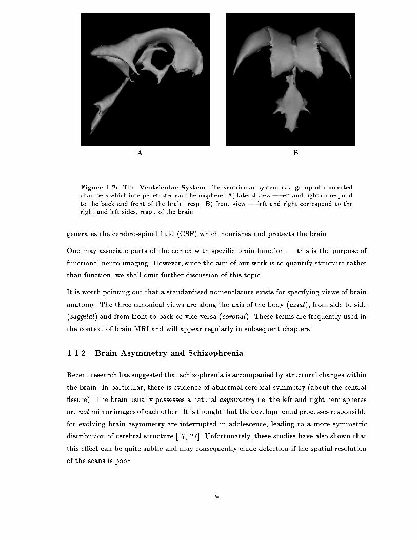
contains additional structures� The largest of these is the ventricular system Figure �� a

network of interconnected chambers which interpenetrates each hemisphere� This structure

�

Figure �� Two Views of the Brain The �rst row shows a top�down axial view� inwhich the two cerebral hemispheres are clearly delineated by the mid�saggital plane� Thesecond row shows a saggital view � note that the cerebellum is included� The asymmetrybetween the left and right hemispheres is readily apparent� The principal brain lobes arealso indicated �The volume rendered images were supplied by the Biomorph Project��

�

The figure originally located here has been removed from this electronic version of the thesis for copyright reasons.

A B

Figure �� The Ventricular System The ventricular system is a group of connectedchambers which interpenetrates each hemisphere� A� lateral view � left and right correspondto the back and front of the brain� resp� B� front view � left and right correspond to theright and left sides� resp�� of the brain�

generates the cerebrospinal �uid CSF� which nourishes and protects the brain�

One may associate parts of the cortex with speci�c brain function � this is the purpose of

functional neuroimaging� However� since the aim of our work is to quantify structure rather

than function� we shall omit further discussion of this topic�

It is worth pointing out that a standardised nomenclature exists for specifying views of brain

anatomy� The three canonical views are along the axis of the body axial�� from side to side

saggital� and from front to back or vice versa coronal�� These terms are frequently used in

the context of brain MRI and will appear regularly in subsequent chapters�

�� Brain Asymmetry and Schizophrenia

Recent research has suggested that schizophrenia is accompanied by structural changes within

the brain� In particular� there is evidence of abnormal cerebral symmetry about the central

�ssure�� The brain usually possesses a natural asymmetry i�e� the left and right hemispheres

are not mirror images of each other� It is thought that the developmental processes responsible

for evolving brain asymmetry are interrupted in adolescence� leading to a more symmetric

distribution of cerebral structure �� Unfortunately� these studies have also shown that

this e�ect can be quite subtle and may consequently elude detection if the spatial resolution

of the scans is poor�

�

The MSP forms the standard reference frame for cerebral laterality measures such as the

relative widths of the brain perpendicular to a given point on the plane�� When one refers to

the symmetry of the brain� one is implicitly assuming a LeftRight LR� measure of this type

� Figure �� Observe that the image presented here has had left and right interchanged�

the view point is located beneath the brain� This re�ection is a natural consequence of the

acquisition protocol and should be borne in mind when examining MRI images� Although

R

Front

Back

L

Figure �� Laterality Measures The mid�saggital line is overlaid on this transverse T�weighted MR image� Observe that left and right are interchanged � this indicates that thescan was acquired from the bottom to the top of the brain� The laterality measure L�R

L�R isoften used to quantify asymmetry w�r�t� this line�

a cursory investigation might suggest otherwise� the cerebrum actually possesses a distinct

asymmetry with respect to the MSP� the brain of a healthy subject displays a signi�cantly

larger left hemisphere than right in the posterior part of the brain� As one moves in an anterior

direction� this relationship decreases and then undergoes a reversal � see Figure �� This

e�ect is sometimes called torsion� since it is believed that there may be a developmental

�torque which produces this skewed tissue distribution�

�� Clinical Studies of Brain Asymmetry

A number of reports have suggested that this natural asymmetry is signi�cantly reduced in

the brains of schizophrenics� Evidence of this phenomenon may be found at several levels

within the brain� from gross lateral changes in the temporal lobe to subtler deformations in

structures such as the hippocampus�

The techniques used to investigate this process are many and varied� For example� in ��

�

-8

-6

-4

-2

0

2

4

6

8

0 1 2 3 4 5 6

Asymmetry IndexStd. Devn.

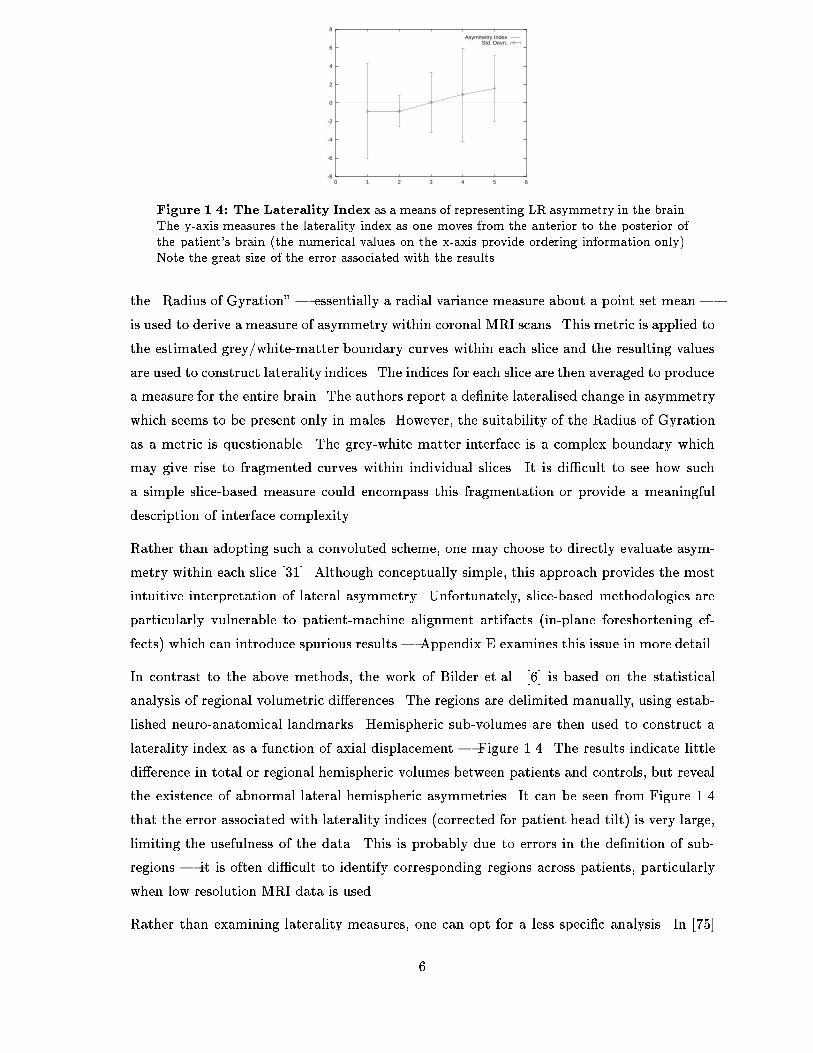
Figure �� The Laterality Index as a means of representing LR asymmetry in the brain�The y�axis measures the laterality index as one moves from the anterior to the posterior ofthe patients brain �the numerical values on the x�axis provide ordering information only��Note the great size of the error associated with the results�

the �Radius of Gyration � essentially a radial variance measure about a point set mean �

is used to derive a measure of asymmetry within coronal MRI scans� This metric is applied to

the estimated grey�whitematter boundary curves within each slice and the resulting values

are used to construct laterality indices� The indices for each slice are then averaged to produce

a measure for the entire brain� The authors report a de�nite lateralised change in asymmetry

which seems to be present only in males� However� the suitability of the Radius of Gyration

as a metric is questionable� The greywhite matter interface is a complex boundary which

may give rise to fragmented curves within individual slices� It is di�cult to see how such

a simple slicebased measure could encompass this fragmentation or provide a meaningful

description of interface complexity�

Rather than adopting such a convoluted scheme� one may choose to directly evaluate asym

metry within each slice �� Although conceptually simple� this approach provides the most

intuitive interpretation of lateral asymmetry� Unfortunately� slicebased methodologies are

particularly vulnerable to patientmachine alignment artifacts inplane foreshortening ef

fects� which can introduce spurious results � Appendix E examines this issue in more detail�

In contrast to the above methods� the work of Bilder et�al� �� is based on the statistical

analysis of regional volumetric di�erences� The regions are delimited manually� using estab

lished neuroanatomical landmarks� Hemispheric subvolumes are then used to construct a

laterality index as a function of axial displacement � Figure �� The results indicate little

di�erence in total or regional hemispheric volumes between patients and controls� but reveal

the existence of abnormal lateral hemispheric asymmetries� It can be seen from Figure ��

that the error associated with laterality indices corrected for patient head tilt� is very large�

limiting the usefulness of the data� This is probably due to errors in the de�nition of sub

regions � it is often di�cult to identify corresponding regions across patients� particularly

when low resolution MRI data is used�

Rather than examining laterality measures� one can opt for a less speci�c analysis� In ��

�

the authors segment the brain into several tissue classes using a semiautomatic thresholding

procedure� They compute global grey and white matter volumes from this segmentation as

well as speci�c cortical volumes for selected subregions� Since there is a well known cor

relation between greymatter reduction and age� the data is normalised to account for this

e�ect� Their �ndings suggest that there are strongly localised greymatter abnormalities in

schizophrenics� In particular� there was a decrease in grey matter in almost all the cortical

regions amongst schizophrenic patients� Once again� however� these results must be inter

preted with some caution� The data used for these measurements is truncated and sparse

which means that corresponding landmarks cannot always be reliably established� An alter

native study of localised greymatter reduction� Shenton et al� �� examined the volume of

greymatter in the temporal lobe and concluded that this volume was reduced in schizophren

ics� However� they also show that the frontal lobe does not exhibit such a reduction� which

contradicts the �ndings of the previous authors�

Although the studies referred to above have all dealt with manifestations of asymmetry�

alternative indices of pathology have been investigated�

A study undertaken by Bullmore �� attempts to quantify the fractal dimension of the grey

white matter interface� with a view to comparing this value for normals and patients� The

analysis is slicebased and the fractal dimension is only able to quantify mean structure�

which is of limited usefulness� An entirely di�erent approach is taken by Kikinis �� the

sulcal patterning of the cerebrum is analysed for pathological indicators� The study used �D

volumetric image processing techniques to produce standardised views of the sulcal patterning

which were then subjected to qualitative and quantitative analysis� These analyses revealed

a distinctive alignment to the sulci of schizophrenic brains� suggesting a neurodevelopmental

aspect to the disease�

While evidence of anomalous asymmetry can be found in other structures such as the ven

tricular system �� the discrepancy between the left and right cerebral hemispheres seems

to be most frequently cited �� as representative of this phenomenon�

�� A Framework for the Segmentation of Sparse MRI

The main contribution of this thesis is the development of a framework for the segmentation

of anatomical structures from sparse MRI� The volumetric images used in this work are

composed of a sequence of �D images� spaced at �mm intervals� each of which represents a slab

of material �mm thick� The resulting lack of structural coherence across neighbouring slices�

suggests that attempts to extract the boundaries of interest using �D voxel segmentation

methods will be unsuccessful� Such schemes operate at the voxel scale� which is unacceptably

�

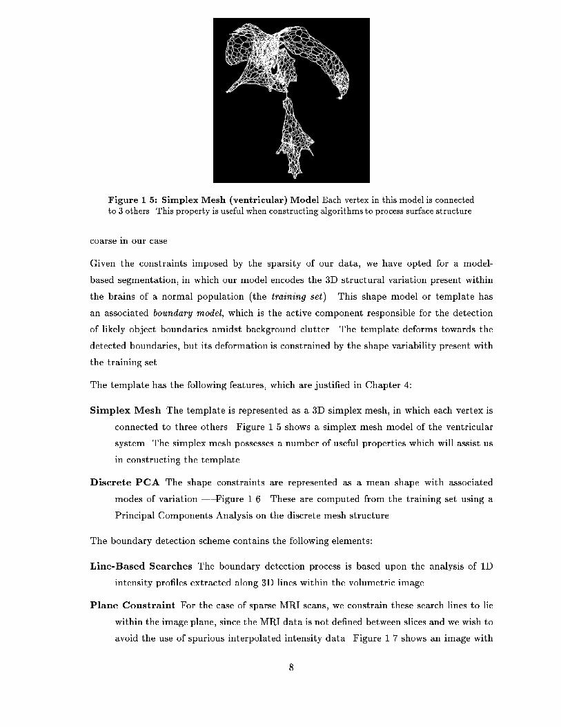
Figure �� Simplex Mesh ventricular Model Each vertex in this model is connectedto � others� This property is useful when constructing algorithms to process surface structure�

coarse in our case�

Given the constraints imposed by the sparsity of our data� we have opted for a model

based segmentation� in which our model encodes the �D structural variation present within

the brains of a normal population the training set�� This shape model or template has

an associated boundary model� which is the active component responsible for the detection

of likely object boundaries amidst background clutter� The template deforms towards the

detected boundaries� but its deformation is constrained by the shape variability present with

the training set�

The template has the following features� which are justi�ed in Chapter ��

Simplex Mesh The template is represented as a �D simplex mesh� in which each vertex is

connected to three others� Figure �� shows a simplex mesh model of the ventricular

system� The simplex mesh possesses a number of useful properties which will assist us

in constructing the template�

Discrete PCA The shape constraints are represented as a mean shape with associated

modes of variation � Figure �� These are computed from the training set using a

Principal Components Analysis on the discrete mesh structure�

The boundary detection scheme contains the following elements�

Line�Based Searches The boundary detection process is based upon the analysis of �D

intensity pro�les extracted along �D lines within the volumetric image�

Plane Constraint For the case of sparse MRI scans� we constrain these search lines to lie

within the image plane� since the MRI data is not de�ned between slices and we wish to

avoid the use of spurious interpolated intensity data� Figure �� shows an image with

�

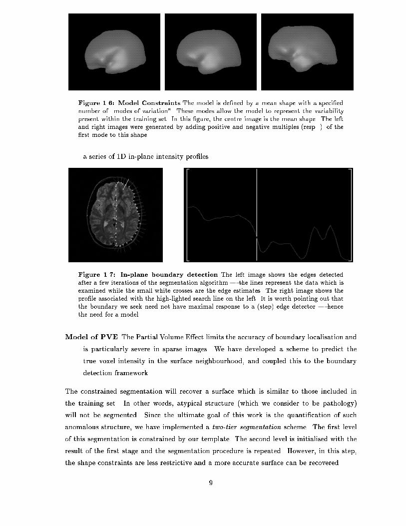
Figure �� Model Constraints The model is de�ned by a mean shape with a speci�ednumber of �modes of variation � These modes allow the model to represent the variabilitypresent within the training set� In this �gure� the centre image is the mean shape� The leftand right images were generated by adding positive and negative multiples �resp� � of the�rst mode to this shape�

a series of �D inplane intensity pro�les�

Figure �� In plane boundary detection The left image shows the edges detectedafter a few iterations of the segmentation algorithm � the lines represent the data which isexamined while the small white crosses are the edge estimates� The right image shows thepro�le associated with the high�lighted search line on the left� It is worth pointing out thatthe boundary we seek need not have maximal response to a �step� edge detector � hencethe need for a model�

Model of PVE The Partial Volume E�ect limits the accuracy of boundary localisation and

is particularly severe in sparse images� We have developed a scheme to predict the

true voxel intensity in the surface neighbourhood� and coupled this to the boundary

detection framework�

The constrained segmentation will recover a surface which is similar to those included in

the training set� In other words� atypical structure which we consider to be pathology�

will not be segmented� Since the ultimate goal of this work is the quanti�cation of such

anomalous structure� we have implemented a two�tier segmentation scheme� The �rst level

of this segmentation is constrained by our template� The second level is initialised with the

result of the �rst stage and the segmentation procedure is repeated� However� in this step�

the shape constraints are less restrictive and a more accurate surface can be recovered�

�

�� Thesis Structure

The thesis is presented as follows�

Chapter Two provides an overview of the MR image acquisition process and details the precise

nature of the data we wish to process� Next� a review of existing segmentation techniques

is undertaken� accompanied by a discussion of their respective shortcomings with respect to

our particular requirements�

Chapter Three introduces snakebased segmentation in the context of sparse data� The

standard �D snake framework is extended to include a priori information and a segmentation

based on propagating planar snakes is developed� The construction of �D surfaces from

this �D data and the extraction of the MidSaggital Plane � required for quanti�cation

of asymmetry � are then investigated� The chapter concludes with a discussion of the

limitations imposed by sparsity and outlines the criteria which an alternative �D scheme

should satisfy�

Chapter Four introduces the Simplex Mesh formalism� We discuss the de�ciencies of the

basic meshsegmentation approach� and show how it can be extended to suit our purposes�

The issues involved in the construction of a mesh shape template are then addressed�

Chapter Five develops the boundary detection scheme which will underpin the segmentation�

Chapter Six proposes a scheme to predict the intensity of voxels which are badly a�ected

by PVE� This framework follows naturally from the boundary modeling scheme developed in

the previous chapter� and provides the basis for more accurate boundary localisation�

Chapter Seven combines the work of previous chapters to arrive at the full segmentation

strategy� The twotier segmentation scheme is evaluated over a number of examples� and a

detailed discussion of the results is presented�

Chapter Eight concludes the thesis� The methodology is reviewed and its shortcomings are

discussed� along with proposals for improvement�

��

Chapter �

Preliminaries

The construction of a robust segmentation scheme requires a thorough understanding of one�s

data� This observation is particularly relevant to magnetic resonance imaging� in which the

protocol determines the image resolution and contrast� and consequently the image features

which may be reliably extracted� This chapter provides the background required to under

stand the issues associated with the segmentation of sparse MRI�

We begin by introducing the basic concepts behind MR imaging� Section �� In Section ��

we provide a more rigorous de�nition of �sparsity and discuss the problems such data poses

for segmentation� A brief review of relevant segmentation schemes is then presented in

Section �� and the chapter concluded in section ��

�� Magnetic Resonance Imaging

Magnetic resonance imaging MRI� is a noninvasive volumetric imaging technology� Al

though there are other volumetric imaging modalities� for example positron emission to

mography PET� and computed tomography CT�� MRI usually� does not require the in

troduction of radioisotopes into the patient�s blood stream� nor does it utilise highenergy

electromagnetic radiation� MRI is characterised by exceptional discrimination of soft tis

sues� which is of great importance for the investigation of tumours and other tissuebased

pathologies�

The technique is based on the phenomenon of nuclear magnetic resonance NMR�� which

has been utilised in chemical analysis since the latter part of the ��s� The imaging ap

plication was �rst proposed by Paul Lauterbur� then of the State University of New York�

in a �� Nature article� It was only a decade later� however� that the �rst MRI machines

were realised� Whilst these machines were primitive by current standards� they revolutionised

medical diagnosis� providing detailed views of the body�s innermost workings�

��

Of course� MRI did not emerge as a fully evolved technology� There are many issues� partic

ularly those pertaining to imaging artifacts� which are only now being addressed� Since the

bulk of our data was acquired some years ago� these problems need to be addressed before

an e�ective analysis can be developed�

�� Nuclear Magnetic Resonance

The nuclei of elements with odd atomic numbers possess an intrinsic nonzero �spin� This

property is the quantum mechanical equivalent of classical angular momentum� which macro

scopic rotating bodies possesses� Quantum mechanics predicts that each nucleus with non

zero spin will possess a number of quantised spin states� the precise number depending on

the characteristics of the nucleus in question� In the case of Hydrogen� there are two such

states� For simplicity� we shall limit our discussion to this element�

Because nuclei have a net positive charge� each has an associated magnetic �eld and� con

sequently� a prescribed magnetic moment� that is� each nucleus behaves as if it were a tiny

magnet rotating about some axis� In an environment with no coherent external magnetic

�elds� the orientations of the magnetic moments will be random and the net magnetic �eld

arising from these magnetic moments will be approximately zero� The introduction of an

external magnetic �eld B has two important consequences�

�� It increases the separation between the low and high energy states of the nuclei which�

according to quantum mechanics� also increases the relative sizes of the populations

inhabiting each of these states � as the �eld strength grows� the lower energy state

becomes more densely populated�

�� It induces precession of the magnetic moments of each nucleus about the applied �eld�

Figure �� The precession is at a frequency� �� speci�ed by the Larmor Equation�

� � � jBj� where � is the gyromagnetic ratio� which di�ers for each element� In thecase of Hydrogen� for example� it has the value �� MHz�Tesla the Tesla is a measure

of magnetic �eld strength��

The excess of nuclei with aligned magnetic moments in the low energy state manifests itself

as a macroscopic magnetisation vector�B�� oriented along the external �eld Figure �� By

further stimulating the sample with a radiofrequency RF� pulse containing the same energy

as that separating the two spin states� we induce a resonance phenomenon which boosts a

proportion of the nuclei into the unstable high energy state� where they remain until the

stimulus is removed� To an external observer� the RF pulse� which is at or near the Larmor

resonance� frequency� �ips the magnetisation vector into the orthogonal transverse� plane

for a �� degree pulse�� Within the transverse plane the magnetisation vector is subject to the

��

Low Energy State

0B

B

Field

HighEnergy State

Net Magnetisation

Magnetic

Figure �� E�ect of a Magnetic Field An external magnetic �eld causes the individualnuclear magnetic moments to precess about it� Because of the discrepancy between the twospin states� a net magnetisation is produced on the macroscopic level� oriented along the�eld�

external �eld� and proceeds to rotate at the Larmor frequency� Since a changing magnetic

�eld induces a current in a length of wire� the strength of rotating magnetisation vector

may be measured by placing a receiver coil in close proximity to the sample� These various

elements are shown in Figure ��

T

T

T

T

MzMoBo Mz

No Signal

Partial Relaxation

MM

t2t1

t=t2t=t1, Mz=0, M =Mo

Mo

M

t

90 deg. RF Pulse

Figure �� RF Resonance and Relaxation A ��o RF pulse at the resonance frequency�ips the magnetisation vector into the transverse plane� where it rotates at the Larmorfrequency� The transverse component� MT � of the magnetisation vector M� � which iswhat our receiver coil detects � is maximal at this point� while the axial component MZ isusually zero� Over time the nuclei revert to the lower energy state and MT decays as themagnetisation spirals back to equilibrium� Because of this �relaxation a decaying alternatingcurrent is detected by the receiver coil� This signal is known as the Free Induction Decay�FID��

Over time� nuclei revert to the low energy state� causing a decay in the magnitude of the

transverse component of the magnetisation� If one looks at the signal detected in the coil� it

appears as a decaying sinusoid� This is known as the free induction decay �FID��

This relaxation is exponential and is characterized by two parameters T� and T�� The �rst

��

governs the growth of longitudinal axial� magnetisation�MZ � while the second characterises

the decay of the transverse component� MT � More formally�

MZ t� � M� MZ ��M��e� t

T� ��

MT t� � MT ��e� t

T� ��

where M� is the equilibrium value of magnetisation vector prior to the pulse� and MT ��

and MZ �� are the initial values after a �� degree pulse� Observe thatMZ �� will not be zero

if the sample has not been permitted to relax completely prior to the next RF pulse�

The precise values of T� and T� are a�ected by� amongst other things� the composition

and temperature of the sample� as well as the strength of the external �eld� These values

determine the contrast in an image� Furthermore� one may accentuate one or the other by

manipulation of the MR imaging parameters� resulting in socalled T� and T� �weighted

images� Contrast and imaging are discussed in the next section�

In practise the RF pulse will have a �nite bandwidth� which means that a range of nuclei will

be stimulated� This produces a composite signal which is a superposition of individual FID�s�

The signal can be decomposed using a Fourier transform� enabling us to recover the individual

frequency components and their magnitudes� This is the basis for NMR Spectroscopy� which

is widely used in chemical analysis�

To overcome e�ects such as sample dephasing� in which the magnetisation vector begins to

decay as the underlying spin states lose coherence� modi�ed acquisition techniques must be

introduced� In spin�echo NMR� the sample is subjected to another radio frequency pulse� of

equal but opposite polarity� This has the e�ect of reversing the phase of all of the components

which constitute the sample� while leaving the precessional direction unchanged� At a speci�c

time� the spin echo time �TE�� all dephasing is reversed and a clear� sharp signal is obtained�

By utilising polarised magnetic gradient �elds� one can induce a functionally identical gradient

echo in the sample� However� this approach is susceptible to �eld inhomogeneities and is

therefore only used in certain special applications� such as rapid imaging�

�� Image Formation

Clinical MRI is usually based on Hydrogen proton� NMR� since this element is present in

almost all tissue types and has the added virtue of providing a strong NMR signal� Since

di�erent tissues have di�ering amounts of water� each will generate a unique signature which

may then be interpreted as an intensity for image formation purposes� Collecting a single

complex signal from a �D volume is only useful for imaging if we can assign spatial coordinates

to the individual frequency components i�e� determine where the signals originated from� Both

��

Transform

X

Yy Fourier

Frequency

Phase

K

ImageK-Space

Kx

A B

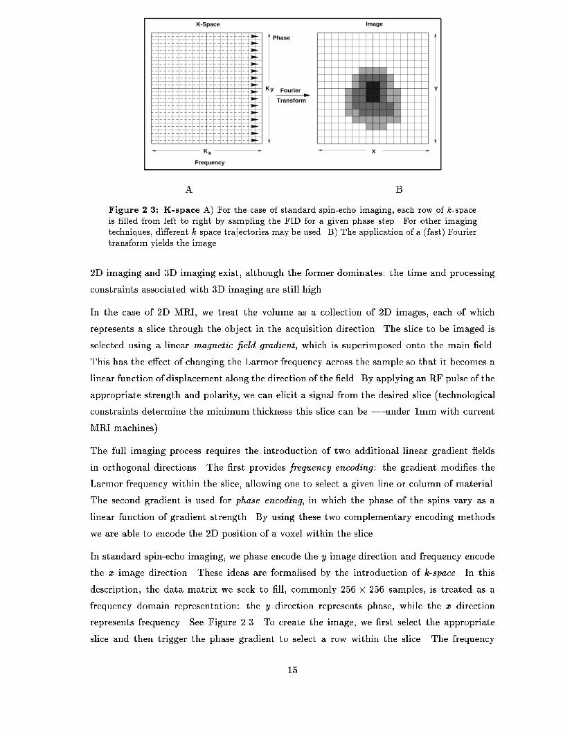
Figure �� K space A� For the case of standard spin�echo imaging� each row of k�spaceis �lled from left to right by sampling the FID for a given phase step� For other imagingtechniques� di�erent k�space trajectories may be used� B� The application of a �fast� Fouriertransform yields the image�

�D imaging and �D imaging exist� although the former dominates� the time and processing

constraints associated with �D imaging are still high�

In the case of �D MRI� we treat the volume as a collection of �D images� each of which

represents a slice through the object in the acquisition direction� The slice to be imaged is

selected using a linear magnetic �eld gradient� which is superimposed onto the main �eld�

This has the e�ect of changing the Larmor frequency across the sample so that it becomes a

linear function of displacement along the direction of the �eld� By applying an RF pulse of the

appropriate strength and polarity� we can elicit a signal from the desired slice technological

constraints determine the minimum thickness this slice can be � under �mm with current

MRI machines��

The full imaging process requires the introduction of two additional linear gradient �elds

in orthogonal directions� The �rst provides frequency encoding � the gradient modi�es the

Larmor frequency within the slice� allowing one to select a given line or column of material�

The second gradient is used for phase encoding� in which the phase of the spins vary as a

linear function of gradient strength� By using these two complementary encoding methods

we are able to encode the �D position of a voxel within the slice�

In standard spinecho imaging� we phase encode the y image direction and frequency encode

the x image direction� These ideas are formalised by the introduction of k�space� In this

description� the data matrix we seek to �ll� commonly �� samples� is treated as afrequency domain representation� the y direction represents phase� while the x direction

represents frequency� See Figure �� To create the image� we �rst select the appropriate

slice and then trigger the phase gradient to select a row within the slice� The frequency

��

gradient is then applied and the signal sampled while the �eld is maintained� The sampled

FID is then copied into a row of the matrix and the phase gradient stepped in preparation

for the next RF excitation� which may be initialised after the system has relaxed back to it�s

equilibrium state� The time� TR� separating excitations is known as the repetition time and

plays a fundamental role in the manipulation of contrast� This value is usually in the range

�� milliseconds�

The process of stepping through the phase gradient would have to be repeated �� times

with the above matrix size� Furthermore� to boost SNR� the number of excitations NEX�

per matrix row may be greater than one� typically two or three� The total time required is

given by

T � NOL �NEX� TR� ��

where NOL represents the number of lines phase steps� in the matrix� It is also possible

to acquire several rows within one repetition time by using a modi�ed spinecho pulse se

quence� This allows one to produces several di�erently weighted� images simultaneously� or

to produce a single image more rapidly� In this case the time required is

T �NOL

NR�NEX � TR ��

where NR is the number of echoes generated within TR�

Once the kspace matrix is assembled� we may apply a discrete Fourier transform to arrive

at a spatial representation� The image is prepared by assigning greyscale intensities to each

voxel that are proportional to the NMR signal originating from that spatial region�

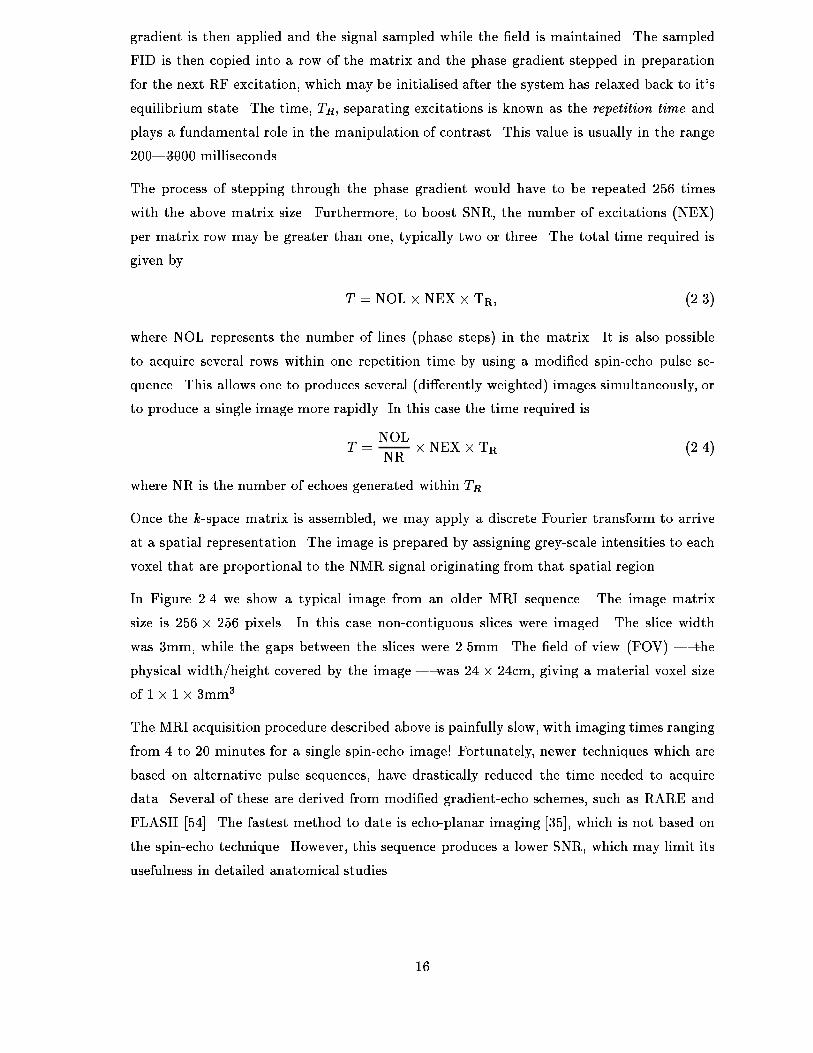
In Figure �� we show a typical image from an older MRI sequence� The image matrix

size is �� pixels� In this case noncontiguous slices were imaged� The slice widthwas �mm� while the gaps between the slices were ��mm� The �eld of view FOV� � the

physical width�height covered by the image � was �� cm� giving a material voxel sizeof �� mm��

The MRI acquisition procedure described above is painfully slow� with imaging times ranging

from � to �� minutes for a single spinecho image� Fortunately� newer techniques which are

based on alternative pulse sequences� have drastically reduced the time needed to acquire

data� Several of these are derived from modi�ed gradientecho schemes� such as RARE and

FLASH �� The fastest method to date is echoplanar imaging �� which is not based on

the spinecho technique� However� this sequence produces a lower SNR� which may limit its

usefulness in detailed anatomical studies�

��

Figure �� AnMRI ImageAn image acquired under an older MRI protocol� the thicknessof the slice is �mm and each image in the sequence is separated by a ��mm gap� The FOVis �� cm�

�� MRI Slice Resolution

During image formation� a gradient magnetic �eld is used to select the volume of material

from which the MR signal is to be acquired� The signal itself is generated by the application

of an RF pulse at the appropriate Larmor frequency� Since the pulse has �nite duration� its

Fourier domain representation will have an associated frequency bandwidth� Consequently�

the gradient �eld will not select an idealised slice in �D� but a slab of material� the thickness

and location of which are determined by the �eld strength and RF bandwidth� Furthermore�

since the RF pulse is usually a Gaussian or truncated sinc function� the frequency response

will not be uniform over the frequency range� Rather� the response will decay rapidly as

one nears the limits of the frequency range� This manifests as a blurring of the selected

volume boundary� since signal information will be captured from adjacent material� To

reduce the overlap between neighbouring slices� consecutive image slabs may be acquired

with an intervening gap� In this case� the gap is made wide enough to ensure that the no

signal contribution arises from adjacent slices� The sparse images used in this thesis are

examples of such acquisitions�

�� MRI Contrast

By adjusting TR� the duration of the RF pulses and the strength of the magnetic �elds�

the relative contrast of tissues within the imaged volume may be modi�ed� Such contrast

modi�cations can provide a signi�cant aid to diagnosis� One can also use contrast agents� such

as Gadolinium DTPA� to enhance speci�c pathology such as tumours� However� by judicious

manipulation of imaging parameters� one can often form a conclusive diagnosis without the

need for invasive indicators�

There are several standard image contrast protocols� each named for the aspect of the NMR

��

IntensityPD T� T�

long TR� short TE short TR� short TE long TR� long TE

High Fat CSFGrey� White Matter Bone Marrow

Fat Grey� White Matter Grey� White MatterCSF Fat

CSFCortical Bone Cortical Bone Cortical Bone

Low Flowing Blood Flowing Blood Flowing Blood

Table �� MRI Contrast Weighting Schemes This table shows the relative brightnessof various tissue types for given MRI contrast weighting schemes� For spin�echo imaging� therepetition time �TR� and the echo time �TE� are the parameters which select the particularimage weighting� the relative sizes of these parameters are indicated in the �rst row of thetable�

signal they most emphasize� For example� in a T��weighted �spin�echo� image� the RF pulse

repetition time is too fast to allow signi�cant relaxation of the magnetisation vector� As

a consequence� tissues with long T� relaxation times will lose contrast relative to those

with shorter times� since the magnetisation will be tilted back into the transverse plane

before having recovered its full strength� Two other popular weighting schemes are T�� the

complement of T�� and Proton Density PD�� which gives an indication of the Hydrogen

density across the image� See Table �� for details reproduced from ��

The spinecho signal intensity is given by

SI � K� �� e��TR�TE�T� e�TET� � ��

where K represents the in�uence of various environmental parameters and � is the proton

density� This equation describes the e�ect of RF pulse timing on the image contrast� and

hence whether the signal is T� or T�weighted�

There is no easy way to determine visually the particular weighting given to an image� since

there is a degree of overlap between each protocol� Certain heuristics may� however� allow

one to make an educated guess� For example� a T�weighted scan will have a high signal

bright intensity� for waterbased substances� such as CSF� while CSF will appear dark on

a T�weighted scan� Protondensity scans are less easily di�erentiated� In the interests of

clarity� we shall explicitly state the weighting scheme whenever we present MRI data�

�� MRI Artifacts

The MR imaging process is susceptible to a number of artifacts which can complicate image

interpretation�

Inhomogeneities in the MR receiver coil and the magnetic �eld can result in a low frequency

��

Figure �� Bias Field This image exhibits a bias �eld artifact� which is caused by inho�mogeneities in the MR receiver coil� The contrast in this image has been manipulated toaccentuate the artifact� �Image courtesy of W� M� Wells� Harvard Medical School�

multiplicative signal� the bias �eld� corrupting the image� An extreme example of this e�ect

is shown in Figure ��

There are also more destructive artifacts� particularly those associated with motion� Patients

are seldom still� each twitch is translated into ghostly blurring or worse �� Examples

of such images are shown in Figure �� Furthermore� the NMR characteristics of a region

may be a�ected by blood �ow and local �eld inhomogeneities� complicating intensity based

analysis further�

A B

Figure �� Imaging Artifacts A� PD�weighted MRI scan with severe motion �ghosting �B� Horizontal bands of noise reveal the presence of rapidly �owing arterial blood in thisT�weighted image�

If the object being imaged is undersampled when the FID is sampled too coarsely� one

may observe aliasing e�ects in the reconstructed data� structures beyond the �eld of view

are erroneously mapped or �folded back into the image� This artifact can be eliminated

during image acquisition by oversampling or increasing the time over which the MR signal is

collected�

��


There are a multitude of other artifacts� but the ones discussed above represent those most

commonly encountered in the data used for this thesis� A more detailed discussion can be

found in Rinck ��

�� Characterisation of Sparse MRI Data

The MRI data we wish to segment was acquired under a long term study of anomalous brain

structure in schizophrenics� Data from such extended clinical studies is rare� and special

segmentation techniques are required to cope with many of the older scans in the series �

the bulk of the data was imaged using old spinecho protocols which have poor resolution

perpendicular to the slice plane� Although there are a number of existing techniques for the

segmentation of high resolution data� these methods would not work well on such coarse data�

hence the need for alternative sparse segmentation techniques� In this section we describe

our data in more detail� as well as describing the problems it poses for segmentation�

�� Sparse MR Images

The term �sparse MR was coined to describe the class of MR images which have a high

sampling rate within each image slice� but a comparatively low sampling rate in the direction

perpendicular to the image plane� Since the image is formed by sampling the FID within the

Fourier domain� the dimensions of the kspace matrix directly determine the scale spatial

frequency� of the structures which can be discerned when the image formationDFT is applied�

The kspace matrix represents a uniform sampling of the Field Of View in the x and y

directions� For example� a �� matrix will yield a poorer more blurred� image thana �� matrix for a �xed size FOV� In sparse images� the sampling rate is su�cientlyhigh to enable structure on the scale of about �mm to be represented within each image�

However� due to the e�ective sampling distance between each slice� the structure is degraded

in a very speci�c way� described in Section �� below� as one moves through the stack of

images� Furthermore� with the large interslice sampling distance used in this work� there

is no possibility of detecting similar �nescale structure in the perpendicular direction� even

when the inplane degradation is minimal�

�� Sparse MR Image Database

The sparse images used in this work are �� or �� slice spinecho images� The image slices

are �mm thick and separated by a gap of �mm� with a typical FOV of �� cm� Theimage matrix size is �� and the number of excitations NEX� is variable� All thestandard contrastweighting schemes T�� PD� T�� are present� but the particular choice was

��

left to the discretion of the radiologist� In certain cases� interleaved PD and T� images were

acquired� The magnet strength used ��T� Both axial and coronal scans are present� with

the former being more numerous� Subjects were imaged at a number of consecutive time

points� The period of the study spanned several years� and high resolution coronal� scans

were introduced near the end of this period� Such temporal MR sequences provide a record

of the progression of the disease�

The age distribution of the subjects ranged from �� with the bulk of the subjects lying

within the lower half of this range� The sex ratio was approximately even� but favoured

males� Handedness was predominantly left�

�� Segmentation Issues

There are a number of issues which are of particular relevance to the segmentation of sparse

data�

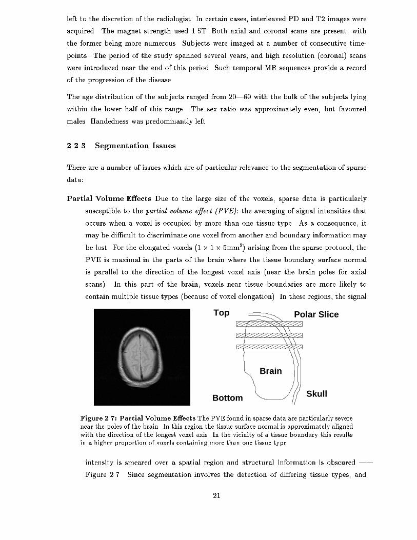
Partial Volume Eects Due to the large size of the voxels� sparse data is particularly

susceptible to the partial volume e�ect �PVE�� the averaging of signal intensities that

occurs when a voxel is occupied by more than one tissue type� As a consequence� it

may be di�cult to discriminate one voxel from another and boundary information may

be lost� For the elongated voxels �� mm�� arising from the sparse protocol� the

PVE is maximal in the parts of the brain where the tissue boundary surface normal

is parallel to the direction of the longest voxel axis near the brain poles for axial

scans�� In this part of the brain� voxels near tissue boundaries are more likely to

contain multiple tissue types because of voxel elongation�� In these regions� the signal

Brain

Top

Bottom Skull

Polar Slice

��

��

��

Figure �� Partial Volume E�ects The PVE found in sparse data are particularly severenear the poles of the brain� In this region the tissue surface normal is approximately alignedwith the direction of the longest voxel axis� In the vicinity of a tissue boundary this resultsin a higher proportion of voxels containing more than one tissue type�

intensity is smeared over a spatial region and structural information is obscured �

Figure �� Since segmentation involves the detection of di�ering tissue types� and

��

these are indicated by di�erent signal intensities� the PVE must be tackled before we

can proceed�

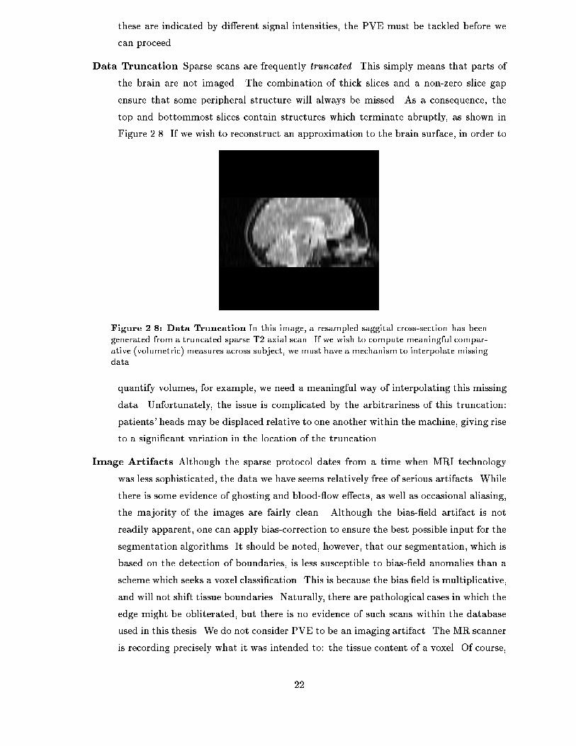
Data Truncation Sparse scans are frequently truncated� This simply means that parts of

the brain are not imaged� The combination of thick slices and a nonzero slice gap

ensure that some peripheral structure will always be missed� As a consequence� the

top and bottommost slices contain structures which terminate abruptly� as shown in

Figure �� If we wish to reconstruct an approximation to the brain surface� in order to

Figure �� Data Truncation In this image� a resampled saggital cross�section has beengenerated from a truncated sparse T� axial scan� If we wish to compute meaningful compar�ative �volumetric� measures across subject� we must have a mechanism to interpolate missingdata�

quantify volumes� for example� we need a meaningful way of interpolating this missing

data� Unfortunately� the issue is complicated by the arbitrariness of this truncation�

patients� heads may be displaced relative to one another within the machine� giving rise

to a signi�cant variation in the location of the truncation�

Image Artifacts Although the sparse protocol dates from a time when MRI technology

was less sophisticated� the data we have seems relatively free of serious artifacts� While

there is some evidence of ghosting and blood�ow e�ects� as well as occasional aliasing�

the majority of the images are fairly clean� Although the bias�eld artifact is not

readily apparent� one can apply biascorrection to ensure the best possible input for the

segmentation algorithms� It should be noted� however� that our segmentation� which is

based on the detection of boundaries� is less susceptible to bias�eld anomalies than a

scheme which seeks a voxel classi�cation� This is because the bias �eld is multiplicative�

and will not shift tissue boundaries� Naturally� there are pathological cases in which the

edge might be obliterated� but there is no evidence of such scans within the database

used in this thesis� We do not consider PVE to be an imaging artifact� The MR scanner

is recording precisely what it was intended to� the tissue content of a voxel� Of course�

��

a mechanismmust still be found to cope with PVE� and we shall suggest such a scheme

later in this thesis�

Image Type The particular contrast scheme T�� T�� PD� and the acquisition direction

axial� coronal� saggital� will both have an e�ect on the algorithms needed to segment

the data� The e�ect of contrast is obvious� the tissue boundary model is directly de

pendent on the image intensities� The role of the acquisition direction is less clear� The

cerebral surface in sparse axial scans appears signi�cantly smoother when compared to

the corresponding coronal view� in the latter case the sulci are clearly visible� revealing

highly convoluted boundary structure� Given the sparsity of the data� the tracking

of individual sulci is not feasible� as there is little continuity from slice to slice� In

the case of axial and to an extent� saggital scans� we may utilise a �clingwrap type

surface which will ignore small declivities� Application of a similar scheme to coro

nal scans could lead to a surface representation which contains features such as cusps�

interpenetrations�

We now examine a number of existing schemes which have been utilised for the task of

segmentation�

�� Overview of Segmentation Methods

There are a number of generic algorithms for tackling the problem of volumetric image seg

mentation� the complexity and robustness of which vary considerably� At the lower end of the

complexity scale are what we have termed voxel�classi�cation schemes which utilise simple

intensity models to segment the data� An example of such a scheme would be voxelintensity

thresholding� To improve the robustness of the segmentation scheme� one requires models

of greater sophistication� In certain cases� intensitybased schemes may result in gross mis

segmentations� such as the disconnected regions for a solid object� unless the algorithm is

augmented by some sort of shape model� We shall call such schemes shape model based� to

emphasize their added functionality� It should be noted that this classi�cation is intended

to provide a context for our own segmentation scheme and may di�er from the �taxonomy

presented by others� More detailed discussions of relevant work will be presented as required�

�� Voxel�Classication Schemes

In many volumetric MRI studies� the image is segmented using a voxel�classi�cation scheme�

in which each voxel is allocated to one of a speci�ed number of tissue classes� Once this

classi�cation has been accomplished� an estimate of tissue volume may be obtained by simply

counting the appropriate voxels and multiplying by the voxel dimensions�

��

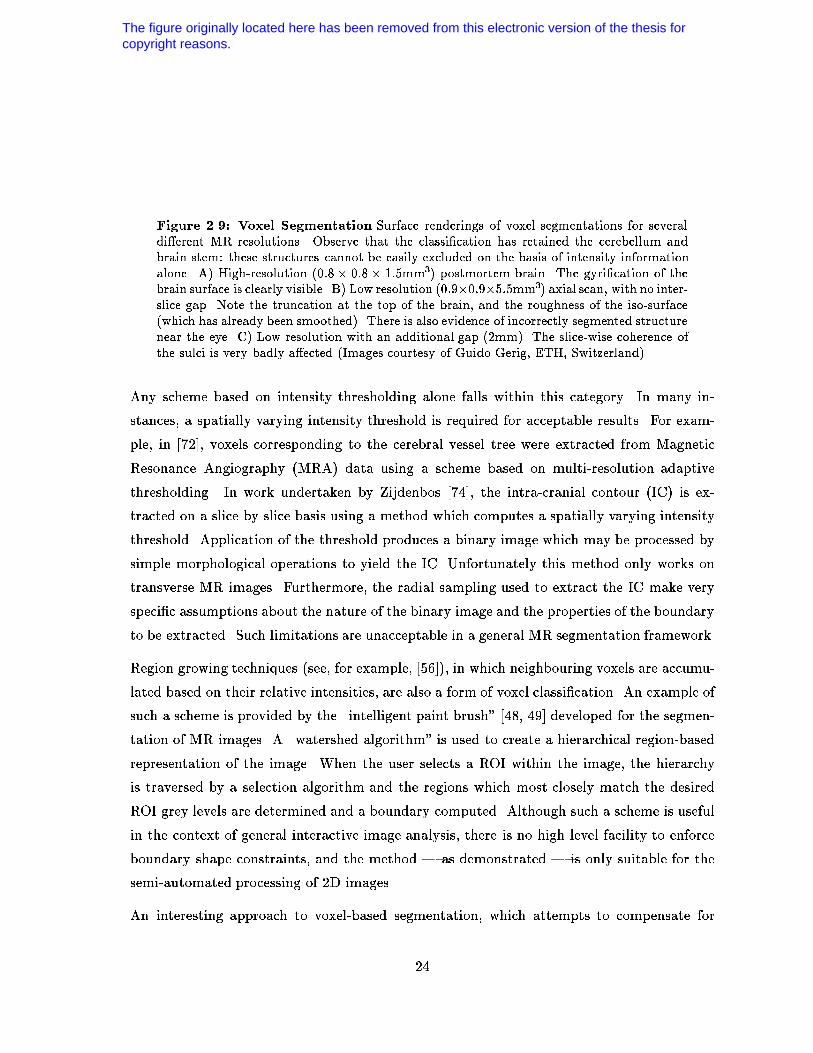
Figure �� Voxel Segmentation Surface renderings of voxel segmentations for severaldi�erent MR resolutions� Observe that the classi�cation has retained the cerebellum andbrain stem� these structures cannot be easily excluded on the basis of intensity informationalone� A� High�resolution �� mm�� postmortem brain� The gyri�cation of thebrain surface is clearly visible� B� Low resolution ��mm�� axial scan� with no inter�slice gap� Note the truncation at the top of the brain� and the roughness of the iso�surface�which has already been smoothed�� There is also evidence of incorrectly segmented structurenear the eye� C� Low resolution with an additional gap ��mm�� The slice�wise coherence ofthe sulci is very badly a�ected �Images courtesy of Guido Gerig� ETH� Switzerland��

Any scheme based on intensity thresholding alone falls within this category� In many in

stances� a spatially varying intensity threshold is required for acceptable results� For exam

ple� in �� voxels corresponding to the cerebral vessel tree were extracted from Magnetic

Resonance Angiography MRA� data using a scheme based on multiresolution adaptive

thresholding� In work undertaken by Zijdenbos �� the intracranial contour IC� is ex

tracted on a slicebyslice basis using a method which computes a spatially varying intensity

threshold� Application of the threshold produces a binary image which may be processed by

simple morphological operations to yield the IC� Unfortunately this method only works on

transverse MR images� Furthermore� the radial sampling used to extract the IC make very

speci�c assumptions about the nature of the binary image and the properties of the boundary

to be extracted� Such limitations are unacceptable in a general MR segmentation framework�

Region growing techniques see� for example� �� in which neighbouring voxels are accumu

lated based on their relative intensities� are also a form of voxel classi�cation� An example of

such a scheme is provided by the �intelligent paint brush �� developed for the segmen

tation of MR images� A �watershed algorithm is used to create a hierarchical regionbased

representation of the image� When the user selects a ROI within the image� the hierarchy

is traversed by a selection algorithm and the regions which most closely match the desired

ROI grey levels are determined and a boundary computed� Although such a scheme is useful

in the context of general interactive image analysis� there is no high level facility to enforce

boundary shape constraints� and the method � as demonstrated � is only suitable for the

semiautomated processing of �D images�

An interesting approach to voxelbased segmentation� which attempts to compensate for

��


the bias �eld artifact� was introduced by Wells and Grimson �� and later extended by

Guillemaud and Brady �� and Brechbuhler et al �� This method uses an Expectation

Maximisation algorithm to iteratively generate a biascorrected voxel classi�cation for a given

number of tissue classes� Unfortunately� it is not always clear a priori how many tissue classes

are required� or how to deal with tissue classes for which the intensity distributions overlap

to a signi�cant degree�

When multimodal image data is available such as PD and T�� one may use data from each

protocol to produce a more robust classi�cation �� This approach assumes that the

images are registered� which need not be the case� patient movement cannot be ruled out

over the scanning period�

The �hierarchical segmentation introduced by Gri�n et al �� uses intensity homogeneity

and �edge strength to build a regionbased image decomposition� Unlike the other schemes

outlined above� this scheme allows one to enforce rudimentary constraints on the segmentation

process� The constraints are posed in terms of pixel membership of overlapping regions� and

are to be supplied by some �higherlevel logic� For medical image segmentation� at least�

such a constraint methodology is of limited usefulness� We require structural constraints

which are not easily codi�ed on a pixel level� and the means by which such constraints are

generated must� of necessity� be speci�ed too�

An iso�surface� constructed from the bounding voxels of a given class segmentation� may

be used to estimate other useful geometric quantities� such as surface area and curvature�

Measures computed from this surface representation are fundamentally limited by the voxel

size�

In its most basic form� MRI voxelclassi�cation assumes�

� Continuity The data are assumed to be contiguous i�e� each voxel is connected along

each face to neighbouring voxels� except along the boundary of the imaged volume� and

� Voxel Class Membership Each voxel may be classi�ed as belonging to a single tissue

class�

For sparse MRI the assumption of continuity is violated since the volumetric images are

sampled so coarsely in the acquisition direction� Furthermore� �corrective voxel interpolation

exacerbates the segmentation problem� since we both increase the e�ective voxel size and

lose intensity information� A little thought will reveal that the second assumption� voxel

class membership� is also violated� sparse data voxels frequently contain signi�cant tissue

contributions from several classes� resulting in an averaged signal� The impact of PVE on the

sparse segmentation problem can be profound� A probabilistic voxel classi�cation method� in

this framework� can do no better than to choose the most likely tissue candidate and classify

��

the voxel accordingly� disregarding the contributions from other classes in the process� Within

the sparse framework� any isosurface approximation based on a voxel level segmentation is

likely to provide a poor estimation of the underlying surface geometry� Voxel segmentations

for high resolution and sparse images are shown in Figure �� Observe that the segmentations

include both the cerebellum and the brain stem� since these are also composed of cortical

matter� The structure of the sulci is badly compromised when the MR data includes an

interslice gap�

An alternative approach� which deviates from the basic paradigm outlined above� is to utilise

a probabilistic hyperstack �� This multiscale representation subdivides voxels to a spec

i�ed level and attempts to predict which higher level structures each subvoxel belongs to�

While this is an interesting idea� the poor resolution of sparse data would make prediction of

structural relationships at a subvoxel scale implausible�

In practice� one needs some sort of underlying model for all but the most trivial segmentations�

This model may� for example� represent the spatial variation of intensity across an object or

serve to delimit permissible variation of a shape� A fundamental limitation of most voxel

based schemes is the lack of structural constraints� given that voxel misclassi�cation is such

a strong possibility� we need a mechanism to reject spurious segmentations�

�� Constraining Shape

The image data we wish to segment may contain missing data or signi�cant image degra

dation� In these cases we may improve the robustness of the segmentation by employing a

deformable model which embodies a priori topological and�or geometric constraints� This

model is usually a surface or contour� with an associated algorithm for extracting shapes of

interest�

Arguably the most popular type of deformable models are active contours or snakes ��

These are energy minimising curves or surfaces in �D� which evolve towards features of

interest in an image or volume�� In �� the features of interest were edges� and the energy

which governed the evolution of the curves was a combination of an internal energy� which

constrained curve �exure� and a imagewide gradient energy� which was maximal in the

vicinity of edges� By choosing an appropriately de�ned energy term� one can select alternative

features of interest� such as textures �� Modi�cations to the basic snake methodology

abound� For example� to tackle the problem of missing data� an expansion term may be

introduced �� which adds an expansive force in the normal direction along the curve�

These ideas may be generalised to �D� although the computational overheads increase and

the additional degree of freedom can complicate or even frustrate implementation� In the

case of �D segmentation� the introduction of a priori knowledge may signi�cantly ease these

��

problems� For example� in �� the authors use a snake surface with an embedded axial

symmetry constraint to segment structures with cylindrical topology� Unfortunately the

brain has a complicated geometry which is not easily modeled�

There are many permutations of the above schemes� For example� Blake et al �� developed

a model which uses a snake formalism complemented by a shape template constraint� only

shapes related to the template by an a�ne transformation are permitted� While the a�ne

constraint is appropriate for the particular context within which the system was proposed�

it would be too restrictive for use in our work� since brain variability has a signi�cant non

linear component� This method also has certain other interesting features� For example� the

global �image potential� which moves the snake towards features of interest� is replaced by

local feature searches and a modi�ed update scheme developed� This reduces computational

overheads and allows one tighter control over local snake evolution�

Parametric surfaces such as superquadrics and their generalisation� hyperquadrics ��

have been widely used as a means of enforcing simple shape constraints on the surface model�

Unfortunately� the complexity of the shapes these models can represent tend to be rather

limited� An interesting approach which provides increased shape discrimination is the use of

free�form deformations �� after a rough segmentation has been achieved with a parametric

surface a superquadric in this case�� However� the number of additional parameters required

to accurately represent a shape grows rapidly as data becomes more complex� limiting its

usefulness for the segmentation of convoluted structures�

The deformable templates introduced in �� employ parametric curves�surfaces to represent

the shapes of interest� The model �tting is accomplished by a global energy minimisation

over the set of shape parameters� This approach is not suitable for the complex geometry of

the brain� obtaining a parametric representation of such a complex object is a rather di�cult

task� Furthermore� such a representation� assuming it could be generated� would require a

large number of parameters resulting in a search space of extremely high dimension�

The deformable Fourier Surfaces introduced by Staib and Duncan �� provide an interest

ing blend of segmentation and analysis functionality� A discrete mesh of simple topology is

decomposed on a Fourier basis� and a vertex update scheme developed which allows a con

strained mesh deformation in the direction of the data points� These ideas were taken further

in the work of Szekely et al �� who applied this deformable surface to the segmentation and

analysis of structures within the brain the corpus callosum and deep grey matter surfaces��

In their work the Fourier descriptors of the �nal surface representation were used for the

investigation of pathology � essentially they use a Euclidean metric to compare vectors of

descriptors from di�erent patients� Unfortunately the Fourier representation requires that

a surface parameterisation be established� Although a method for obtaining a surface pa

��

rameterisation was suggested by Brechbuhler �� only closed surfaces with no holes may be

processed� This means that the ventricular system� for example� cannot be decomposed onto

a Fourier basis using this method� We desire a scheme which can represent complex objects

with potentially� many holes�

The lack of a general surface parameterisation scheme for arbitrary topologies means that

the techniques discussed above are fundamentally limited� A number of �nonparametric

methods have been developed to address this issue� For example� the �implicit deformable

model introduced by Whitaker �� is based on a discrete surface model which evolves under

a series of di�erential equations� In a somewhat di�erent vein� the topological snakes of

McInerney et al �� are de�ned on a �simplicial grid of �xed resolution� By decomposing

the polygonal snake curve onto the simplicial grid� the evolving snake contours can be made

to merge or split under the action of image forces� While such a simplicial grid may be

generalised to �D� as the authors have shown� there is no easy mechanism to enforce shape

constraints� the curves or surfaces will evolve to �t the most likely edge candidates those

selected by the image potential�� If there is a high level of images noise� or edge degradation�

a poor segmentation is likely�

The most common nonparametric schemes involve the direct evolution of a vertex set repre

senting points on an underlying surface for which no parameterisation implicit or otherwise�

is assumed� There are a number of schemes based on surface triangulations under which

the mesh vertices evolve in a snakelike fashion towards feature points in the volume� The

vertices are usually assumed to be connected by a series of perfect springs� and the appro

priate Newtonian force model is invoked see� for example� �� A closely related approach

developed by Nastar and Ayache �� adds �volumetric springs vertex connections through

the volume� to increse stability and better model the object properties� They also utilise

a modal analysis a multiscale basis decomposition� similar to Fourier decomposition� to

obtain a compact set of shape descriptors which may be used for subsequent analysis� While

this approach is very general� there is no mechanism to enforce shape constraints a shape

model�� and because of the nonlocality of the volumetric springs� local perturbations may

a�ect distant parts of the mesh�

The most serious shortcoming of the segmentation schemes discussed above is the lack of

an explicit shape constraint� This constraint or model� should encode shape geometry and

topology for surfaces with complex structures� whilst being su�ciently general to represent

the variability present within the shape class�

An elegant approach encompassing shape model construction and segmentation is the active

shape model ASM� introduced by Cootes et al �� By examining a set of

normalised training shapes one can build a point distribution model PDM� which encodes

��

the shape class variability� The model is a discrete representation in which every point has

an associated mean and variance that constrain its displacement� The PDM is the result of

performing a principal components analysis on the set of corresponding points� This yields

the dominant �shape modes which span a reduced linear subspace within which learned

shapes may be represented with only a few parameters basis or modal coe�cients�� This

modal representation provides a simple framework to compare shapes within the class� via

their modal coe�cients�

A more recent technique uses a simplex mesh �� a discrete surface model composed of

vertices with �connectivity� to represent the shape model� This model deforms under the

action of image and internal forces� If data is not available the a�ected region tends to relax

towards the shape de�ned by the template� There is also a well de�ned set of local mesh

transformations which enable one to dynamically modify the topology and nodedensity of

the template� The �connectivity property ensures that one can derive simple and symmetric

algorithms to process the mesh structure� Like some of the other meshbased segmentation

schemes presented above� the simplexmesh is governed by a Newtonian force model� However�

the internal forces acting on the model are local and can be forced to respect an overall shape

constraint ��

The simplex mesh framework provides a very general infrastructure for shape representation

which includes local surface updates and a complex shape model� However� it does not address

the issue of shape model variability or the detection of boundary data in a degraded image

such as sparse MRI�� The ASM addresses the issue of shape variability through a training

process� but does not specify any particular mesh representation� and likewise assumes that

boundary detection is near� trivial� The ASM also assumes that only shapes within or very

similar to� the training set are valid� This is not necessarily the case if pathological structures

are to be segmented� By combing the di�erent shape model capabilities of both schemes� and

addressing the issues involved in boundary detection within sparse images� we believe that a

fairly general� robust sparse segmentation scheme can be developed� The active shape model

and simplex mesh will be examined in considerably more detail in Chapter ��

�� Conclusion

Magnetic resonance imaging permits a wide choice of acquisition protocols� These protocols

determine scan attributes such as contrast and resolution and have a profound impact on

the strategies one can utilise to segment them� In the case of sparse data the combination of

truncation artifacts� slice gaps and large voxel size confound generic segmentation schemes�

However� a synthesis of existing schemes augmented by domain speci�c knowledge can allow

us to overcome these limitations� The key aspect of this new methodology is the develop

��

ment of robust shape models that can provide a meaningful extrapolation of missing object

boundary data� The modelling process must be �exible enough to represent the extensive

variability present in biological structures� whilst maintaining a level of detail which is ap

propriate to the sparseness of the data� We now turn our attention to the development of

such a framework� starting with the evaluation of a �D snakebased segmentation strategy�

��

Chapter �

Snakes

An MR image is composed of a stack of �D images� each of which represents a crosssection

through the object of interest as one steps along the imaging axis� If the distance separating

these images is su�ciently large it no longer makes sense to view the scan as a volumetric

entity� it is a composite of �D crosssections� Since the segmentation of a �D image is often

computationally cheaper and more tractable than that of a volumetric image� this alternative

interpretation is appealing� Of course� these images are not entirely independent� and it would

be foolish to ignore this a priori knowledge�

Inspection of high resolution MR data reveals that �� scanned objects produce closed in

tersection curves in the imaging plane and �� these contours are geometrically similar over

adjacent slices� in the sense that their gross shape and location exhibit only small changes�

This structural coherence still exists� although somewhat tenuously� in the case of sparse

MR images� Our segmentation strategy should capture both these elements� If we were

able to reliably determine boundary pixels� we could connect them to produce the curve we

desire� Unfortunately� image noise and artifacts such as PVE make such a scheme infeasible�

Furthermore� such pixel�voxel based schemes are not amenable to the introduction of shape

constraints which limits their usefulness� However� if we utilise a socalled snake contour

model we may simultaneously address the issue of boundary detection and representation�

the snake contour will gravitate towards features of interest in the image the boundary� in

this case�� Additionally� the snake possesses intrinsic regularising properties which enable it

to provide a smooth approximation to the boundary in the presence of image noise�

Given these considerations we decided to implement a snake segmentation scheme� aug

mented to include our adjacency constraint� This constraint is implicitly utilised through

a curve propagation strategy� under which snakes representing the boundaries of interest in

a given image are used to initialise the search in the following image� The slice contours

extracted using this approach may be used to generate a �D surface representation suitable

for calculating symmetry metrics�

��

This chapter describes the implementation and evaluation of such a scheme�

�� The Snake Framework

A snake is an elastic model for shape which can be coupled to image features� Snakes were

originally developed �� as �active contours which move under a combination of �internal

elastic forces and �external forces arising from image features� such as edges� A number

of modi�ed snake schemes have since been devised which are not only more e�cient but also

have more sophisticated methods of incorporating a priori information ��

In the original formulation� the snake was interpreted as the solution to a global variational�

minimisation problem� This approach requires the de�nition of an �image potential to act

as an attractor for the snake� Such a scheme provides only rudimentary shape constraints�

through implicit continuity conditions� An alternative scheme which addresses both compu

tational complexity and the addition of a shape model was proposed in �� In this framework

the snake is explicitly represented as an approximating B�spline cf� Appendix A�� which

has the following features�

Template A shape model or template may be incorporated into the update process� This

model constrains snake deformation in a prescribed way! in the original work only a�ne

deformations of the template were permitted�

Local Computations Rather than using a �potential image to represent features of in

terest� a local feature search is introduced� For the detection of edges� a line of pixels

normal to the spline curve is extracted at speci�ed points along its length� More specif

ically� the polynomial �spans which constitute the snake are uniformly sampled and

these points used as the origins for the pro�le extraction� A �D edge search is then

performed within each intensity pro�le and the location of any edge candidates within

these lines are noted� If a su�cient number of edge candidates are deemed �good

over a given span� that portion of the snake is considered to be locked onto the data

and these points will participate in the update process� The update is implemented by

re�tting the spline curve to the set of locked points� subject to the model constraints�

As a consequence of this locality� the update process reduces to a sparse matrix system

which may be solved rapidly�

Closed form expressions The use of such approximating spline snakes allows the use of

analytic expressions� for example based on Green�s theorem� for computing geometric

quantities such as length� curvature and area � Appendix A�� These quantities can be

obtained e�ciently and directly from expressions involving only the control points ��

Although these expressions are also available for interpolating snakes� they are not as

��

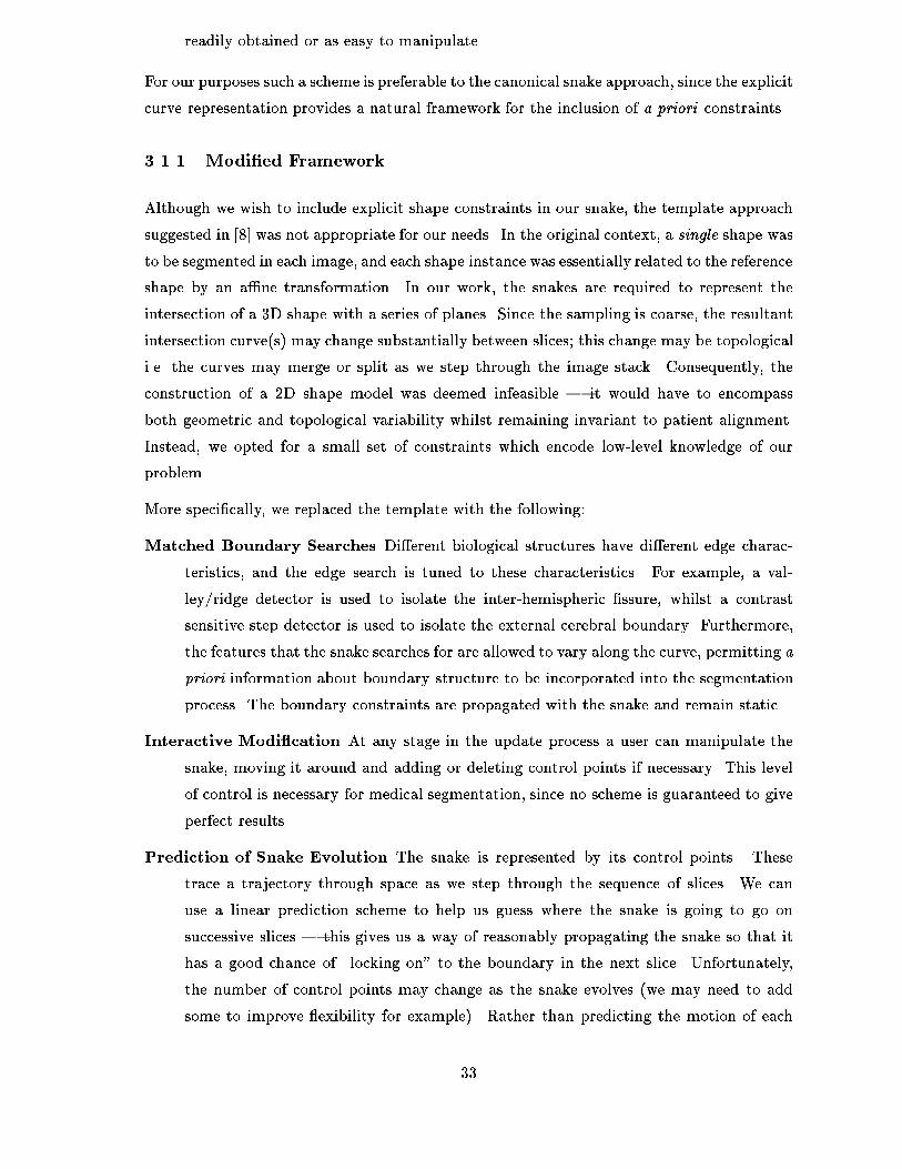
readily obtained or as easy to manipulate�

For our purposes such a scheme is preferable to the canonical snake approach� since the explicit

curve representation provides a natural framework for the inclusion of a priori constraints�

�� Modied Framework

Although we wish to include explicit shape constraints in our snake� the template approach

suggested in �� was not appropriate for our needs� In the original context� a single shape was

to be segmented in each image� and each shape instance was essentially related to the reference

shape by an a�ne transformation� In our work� the snakes are required to represent the

intersection of a �D shape with a series of planes� Since the sampling is coarse� the resultant

intersection curve s� may change substantially between slices! this change may be topological

i�e� the curves may merge or split as we step through the image stack� Consequently� the

construction of a �D shape model was deemed infeasible � it would have to encompass

both geometric and topological variability whilst remaining invariant to patient alignment�

Instead� we opted for a small set of constraints which encode lowlevel knowledge of our

problem�

More speci�cally� we replaced the template with the following�

Matched Boundary Searches Di�erent biological structures have di�erent edge charac

teristics� and the edge search is tuned to these characteristics� For example� a val

ley�ridge detector is used to isolate the interhemispheric �ssure� whilst a contrast

sensitive step detector is used to isolate the external cerebral boundary� Furthermore�

the features that the snake searches for are allowed to vary along the curve� permitting a

priori information about boundary structure to be incorporated into the segmentation

process� The boundary constraints are propagated with the snake and remain static�

Interactive Modi�cation At any stage in the update process a user can manipulate the

snake� moving it around and adding or deleting control points if necessary� This level

of control is necessary for medical segmentation� since no scheme is guaranteed to give

perfect results�

Prediction of Snake Evolution The snake is represented by its control points� These

trace a trajectory through space as we step through the sequence of slices� We can

use a linear prediction scheme to help us guess where the snake is going to go on

successive slices � this gives us a way of reasonably propagating the snake so that it

has a good chance of �locking on to the boundary in the next slice� Unfortunately�

the number of control points may change as the snake evolves we may need to add

some to improve �exibility for example�� Rather than predicting the motion of each

��

control point� we predict the motion of the centroid of the control points as well as the

relative expansion of the snakes as determined by the ratio of their areas�� This is an

unsophisticated global measure� but if we wish to decouple the prediction step from the

actual representation such a compromise seems inevitable�

�� Segmentation

The modi�ed snake framework outlined above served as the basis for a segmentation and

measurement system which is currently in clinical use� The various components of this

system are described below�

�� Initialisation Issues

The snake is initialised on the �rst slice of interest and allowed to propagate across slices�

with possible intervention by the user� There are several issues which need to be addressed

before the process can be initialised�

Control point density The continuity conditions imposed on the Bspline snake implicitly

constrain its shape� When laying down the curve� we must be sure to place su�cient control

points to allow the snake the �exibility it requires to represent the boundaries of interest� If we

have too many control points we essentially lose all regularisation each control point adds two

degrees of freedom�� so some sort of balance must be struck� In the scheme we have developed�

the operator delineated the initial boundary and control points were spaced regularly along

its length� The default spacing could be manipulated if required� Alternatively� the snake

could be de�ned by directly placing control points on the image and moving them about�

This approach was preferred by the clinicians who used the software�

Sample line density The number of sampling lines per span was determined empirically

and was static once selected� The number was set to be three or four� The control point

density also a�ects the e�cacy of the edge searches� if we have too many edge searches in a

region where the control point density is high� then we increase computational time in return

for little improvement�

Snake labelling For the boundaryspeci�c edge searches to be used� the operator must

highlight sections of the curve and indicate which boundary type they correspond to� This

must be done for each intersecting contour� but is only required when a new snake is created�

��

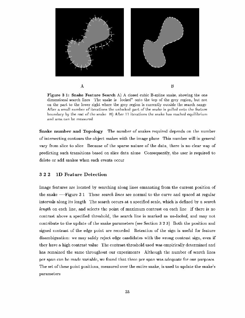
A B

Figure �� Snake Feature Search A� A closed cubic B�spline snake� showing the onedimensional search lines� The snake is �locked onto the top of the grey region� but noton the part to the lower right where the grey region is currently outside the search range�After a small number of iterations the unlocked part of the snake is pulled onto the featureboundary by the rest of the snake� B� After iterations the snake has reached equilibriumand area can be measured�

Snake number and Topology The number of snakes required depends on the number

of intersecting contours the object makes with the image plane� This number will in general

vary from slice to slice� Because of the sparse nature of the data� there is no clear way of

predicting such transitions based on slice data alone� Consequently� the user is required to

delete or add snakes when such events occur�

�� D Feature Detection

Image features are located by searching along lines emanating from the current position of

the snake � Figure �� These search lines are normal to the curve and spaced at regular

intervals along its length� The search occurs at a speci�ed scale� which is de�ned by a search

length on each line� and selects the point of maximum contrast on each line� If there is no

contrast above a speci�ed threshold� the search line is marked as un�locked� and may not

contribute to the update of the snake parameters see Section �� Both the position and

signed contrast of the edge point are recorded� Retention of the sign is useful for feature

disambiguation� we may safely reject edge candidates with the wrong contrast sign� even if

they have a high contrast value� The contrast threshold used was empirically determined and

has remained the same throughout our experiments� Although the number of search lines

per span can be made variable� we found that three per span was adequate for our purposes�

The set of these point positions� measured over the entire snake� is used to update the snake�s

parameters�

��

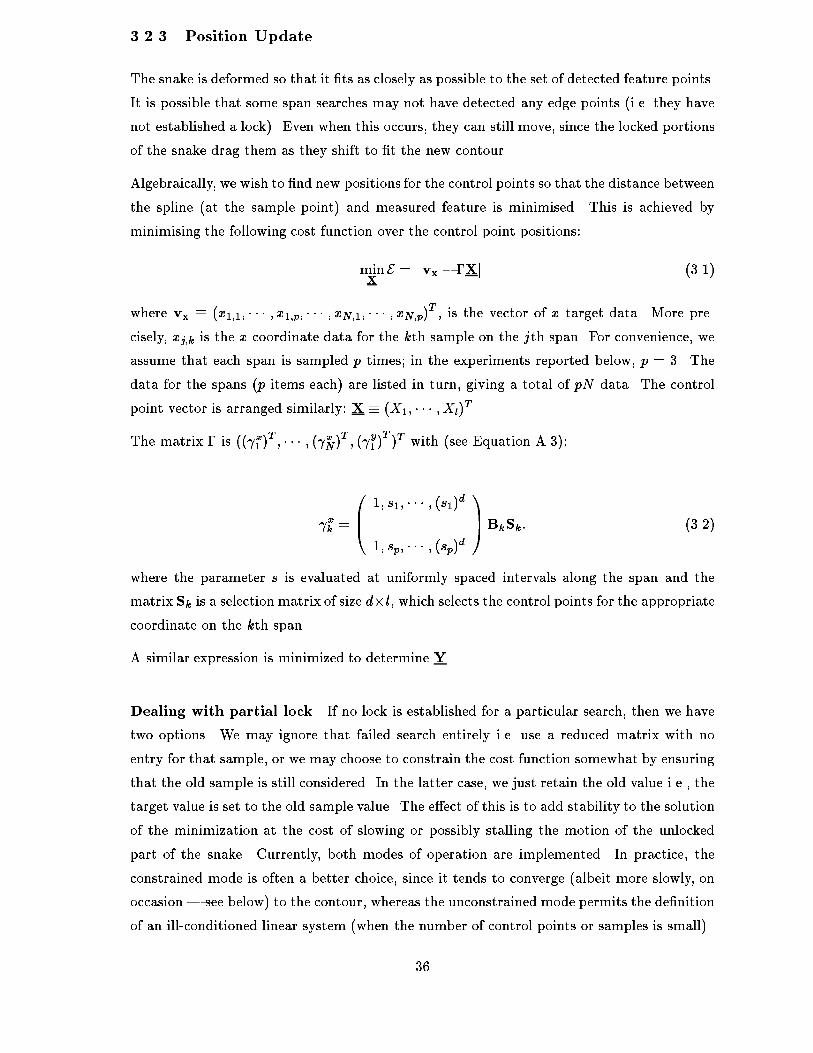
�� Position Update

The snake is deformed so that it �ts as closely as possible to the set of detected feature points�

It is possible that some span searches may not have detected any edge points i�e� they have

not established a lock�� Even when this occurs� they can still move� since the locked portions

of the snake drag them as they shift to �t the new contour�

Algebraically� we wish to �nd new positions for the control points so that the distance between

the spline at the sample point� and measured feature is minimised� This is achieved by

minimising the following cost function over the control point positions�

minXE � kvx � "Xk ��

where vx � x�� x��p� � � � � xN�� xN�p�T � is the vector of x target data� More pre

cisely� xj�k is the x coordinate data for the kth sample on the jth span� For convenience� we

assume that each span is sampled p times! in the experiments reported below� p � �� The

data for the spans p items each� are listed in turn� giving a total of pN data� The control

point vector is arranged similarly� X � X�� Xl�T �

The matrix " is �x��T � � � � � �xN�T � �y��T �T with see Equation A��

�xk �

�B�� s�� s��d

�� sp� � � � � sp�d

�CABkSk� ��

where the parameter s is evaluated at uniformly spaced intervals along the span and the

matrix Sk is a selection matrix of size d�l� which selects the control points for the appropriatecoordinate on the kth span�

A similar expression is minimized to determine Y�

Dealing with partial lock If no lock is established for a particular search� then we have

two options� We may ignore that failed search entirely i�e� use a reduced matrix with no

entry for that sample� or we may choose to constrain the cost function somewhat by ensuring

that the old sample is still considered� In the latter case� we just retain the old value i�e�� the

target value is set to the old sample value� The e�ect of this is to add stability to the solution

of the minimization at the cost of slowing or possibly stalling the motion of the unlocked

part of the snake� Currently� both modes of operation are implemented� In practice� the

constrained mode is often a better choice� since it tends to converge albeit more slowly� on

occasion � see below� to the contour� whereas the unconstrained mode permits the de�nition

of an illconditioned linear system when the number of control points or samples is small��

��

The cost function E in Equation �� can be minimized using a pseudoinverse�

X � "�"��"�vx ��

In this case� minimization of the expression for Y involves application of the same matrix� so

it need not be recomputed�

However� such a �one jump solution may not be optimal� since part of the snake may not

have locked onto a target� It is often better to iterate towards the feature the snake pulls

other regions of itself closer to the edge� allowing them to establish lock� � see Figure ��

Such a scheme may be formalised by the following recursion relation�

Xm�� Xm � #X�m ��

where � � � � � and #X�m � Xp � Xm� The predicted solution� Xp� is obtained by

evaluating Equation �� with the updated target edge data� The parameter � determines the

rate at which the snake converges towards the solution� We used a value in the range �� to

��

Rather than solving the equation directly which requires computation of a large inverse��

we employed GaussSeidel iteration to approximate the solution to "�"�X � "�vx� Since

"�" is sparse block circulant�� the matrix operations may be implemented very cheaply�

�� Correspondence Over Slices

In moving from one slice to another� a natural initial position for the snake is the converged

position from the previous layer� However� the overall size and location of the contour of

interest may change signi�cantly between layers� and our search scale may be too small

encompass this displacement� There is then an increased likelihood that the snake will lock

onto a spurious boundary� By predicting the position of the snake on the next slice one can

provide a reasonable initialisation which reduces the chance of a false lock�

We used a linear recursive �lter �� to update two parameters which controlled the subsequent

positioning of the snake on the next slice� These parameters were the centroid x� y� of

the contour and the relative scaling between layers measured by the area ratio� about the

centroid� The predicted curve position on the next slice was obtained by scaling the snake

about the current centroid and then translating it to the predicted centroid location� Once

the snake had established lock� the updated parameters were fed back into the update and

a new prediction made for the next slice� Initial model parameters were not learned � they

will vary signi�cantly depending on the slice from which the segmentation was initialised�

Instead� user intervention was required to guide the initial segmentation� Once a su�cient

number of slices had been segmented� the prediction was activated and one iteration of the

��

segmentation algorithmwas run every time the user stepped to the next slice� If the prediction

was su�ciently good� no further intervention was required by the user� since the snake would

immediately lock onto the relevant boundary�

�� Results

Figure �� shows the the �nal snake positions after a single snake was initialised and allowed

to propagate across the set of slices� The measured centroid and scaling as the snake tracks

through the sequence� attracted to the right hemisphere� is shown in Figure �� These

measurements are for a sequence where no prediction is used� and the �nal position of the

snake is checked and corrected interactively�

Figure �� a� shows the measured mean distance of the target contour measured from the

initial position of the snake inherited from the previous layer� The starting position is slice ��

Because the brain is roughly hemispherical� the initial distances are small at the �equatorial

sections� and increase at the highly curved upper region� The measured centroid and scaling

functions are used to set the initial parameters of a linear recursive �lter� With the predictive

�lter the measured mean distance is substantially reduced Figure �� b�� A small search

scale can be used and matching between layers is automatic� Note� the scale on the second

�gure was halved to show more detail on the graph��

�� Surface Construction and Mid�Saggital Plane Estimation

Although the segmentation provides a representation of the �D object� this representation

needs to undergo additional processing before we may properly use it� As we have stated

elsewhere� the patient�s brain need not be aligned with the imaging axes of the MR machine�

In order to produce laterality estimates which are free from foreshortening e�ects we must

compute our measures relative to the �D MSP� This involves two steps�

�� MSP estimation

�� Surface construction�

Further discussion of these tasks may be found in ��

�� MSP Estimation

The MSP is most readily identi�ed over the upper part of the cerebrum� where it is de�ned

as the centre of the interhemispheric� �ssure separating the hemispheres before they fuse

lower down�� Although the hemispheric divide is not properly planar over its entire extent�

a plane serves as a good approximation�

��

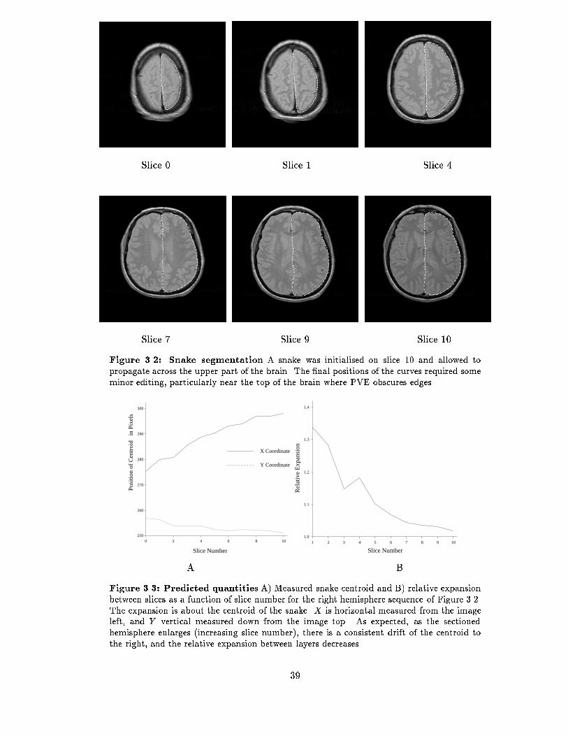
Slice � Slice � Slice �

Slice � Slice � Slice ��

Figure �� Snake segmentation A snake was initialised on slice � and allowed topropagate across the upper part of the brain� The �nal positions of the curves required someminor editing� particularly near the top of the brain where PVE obscures edges�

250

260

270

280

290

300

0 2 4 6 8 10

Slice Number

Posi

tion

of C

entr

oid

Y Coordinate

X Coordinate

in P

ixel

s

1.0

1.1

1.2

1.3

1.4

1 2 3 4 5 6 7 8 9 10

Slice Number

Rel

ativ

e E

xpan

sion

A B

Figure �� Predicted quantities A� Measured snake centroid and B� relative expansionbetween slices as a function of slice number for the right hemisphere sequence of Figure ��The expansion is about the centroid of the snake� X is horizontal measured from the imageleft� and Y vertical measured down from the image top� As expected� as the sectionedhemisphere enlarges �increasing slice number�� there is a consistent drift of the centroid tothe right� and the relative expansion between layers decreases�

��

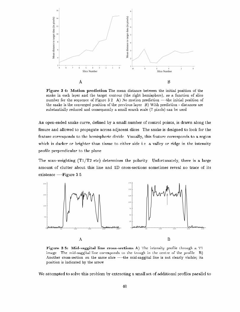
2

4

6

8

10

12

14

16

59 8 7 6 4 3 2 1 0

Slice Number

Mea

n di

stan

ce to

targ

et d

ata

(in

pixe

ls)

1

2

3

4

5

6

7

8

Mea

n di

stna

ce to

targ

et d

ata

(in

pixe

ls)

010 28 6 4

Slice Number

A B

Figure �� Motion prediction The mean distance between the initial position of thesnake in each layer and the target contour �the right hemisphere�� as a function of slicenumber for the sequence of Figure �� A� No motion prediction � the initial position ofthe snake is the converged position of the previous layer� B� With prediction � distances aresubstantially reduced and consequently a small search scale �� pixels� can be used�

An openended snake curve� de�ned by a small number of control points� is drawn along the

�ssure and allowed to propagate across adjacent slices� The snake is designed to look for the

feature corresponds to the hemispheric divide� Visually� this feature corresponds to a region

which is darker or brighter than tissue to either side i�e� a valley or ridge in the intensity

pro�le perpendicular to the plane�

The scanweighting T��T� etc� determines the polarity� Unfortunately� there is a large

amount of clutter about this line and �D crosssections sometimes reveal no trace of its

existence � Figure ��

50 100 150 200 250

50

100

150

200

50 100 150 200 250

25

50

75

100

125

150

175

A B

Figure �� Mid saggital line cross sections A� The intensity pro�le through a Timage� The mid�saggital line corresponds to the trough in the centre of the pro�le� B�Another cross�section on the same slice � the mid�saggital line is not clearly visible� itsposition is indicated by the arrow�

We attempted to solve this problem by extracting a small set of additional pro�les parallel to

��

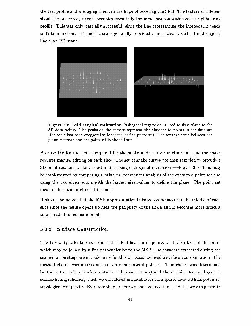
the test pro�le and averaging them� in the hope of boosting the SNR� The feature of interest

should be preserved� since it occupies essentially the same location within each neighbouring

pro�le� This was only partially successful� since the line representing the intersection tends

to fade in and out� T� and T� scans generally provided a more clearly de�ned midsaggital

line than PD scans�

Figure �� Mid saggital estimation Orthogonal regression is used to �t a plane to the�D data points� The peaks on the surface represent the distance to points in the data set�the scale has been exaggerated for visualisation purposes�� The average error between theplane estimate and the point set is about mm�

Because the feature points required for the snake update are sometimes absent� the snake

requires manual editing on each slice� The set of snake curves are then sampled to provide a

�D point set� and a plane is estimated using orthogonal regression � Figure �� This may

be implemented by computing a principal component analysis of the extracted point set and

using the two eigenvectors with the largest eigenvalues to de�ne the plane� The point set

mean de�nes the origin of this plane�

It should be noted that the MSP approximation is based on points near the middle of each

slice since the �ssure opens up near the periphery of the brain and it becomes more di�cult

to estimate the requisite points�

�� Surface Construction

The laterality calculations require the identi�cation of points on the surface of the brain

which may be joined by a line perpendicular to the MSP� The contours extracted during the

segmentation stage are not adequate for this purpose� we need a surface approximation� The

method chosen was approximation via quadrilateral patches� This choice was determined

by the nature of our surface data serial crosssections� and the decision to avoid generic

surface �tting schemes� which we considered unsuitable for such sparse data with its potential

topological complexity� By resampling the curves and �connecting the dots we can generate

��

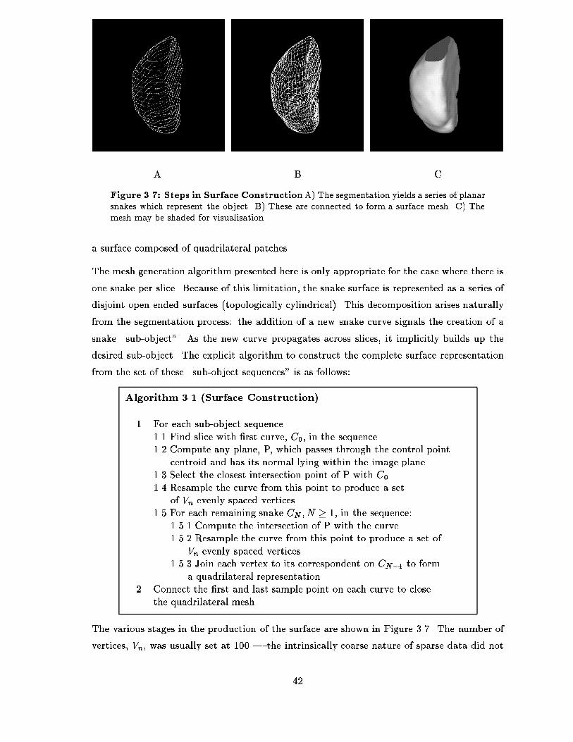
A B C

Figure �� Steps in Surface ConstructionA� The segmentation yields a series of planarsnakes which represent the object� B� These are connected to form a surface mesh� C� Themesh may be shaded for visualisation�

a surface composed of quadrilateral patches�

The mesh generation algorithm presented here is only appropriate for the case where there is

one snake per slice� Because of this limitation� the snake surface is represented as a series of

disjoint open ended surfaces topologically cylindrical�� This decomposition arises naturally

from the segmentation process� the addition of a new snake curve signals the creation of a

snake �subobject� As the new curve propagates across slices� it implicitly builds up the

desired subobject� The explicit algorithm to construct the complete surface representation

from the set of these �subobject sequences is as follows�

Algorithm � � �Surface Construction�

�� For each subobject sequence�� Find slice with �rst curve� C�� in the sequence�� Compute any plane� P� which passes through the control point

centroid and has its normal lying within the image plane�� Select the closest intersection point of P with C�� Resample the curve from this point to produce a set

of Vn evenly spaced vertices�� For each remaining snake CN � N � �� in the sequence�

�� Compute the intersection of P with the curve�� Resample the curve from this point to produce a set of

Vn evenly spaced vertices�� Join each vertex to its correspondent on CN�� to form

a quadrilateral representation�� Connect the �rst and last sample point on each curve to close

the quadrilateral mesh�

The various stages in the production of the surface are shown in Figure �� The number of

vertices� Vn� was usually set at �� the intrinsically coarse nature of sparse data did not

��

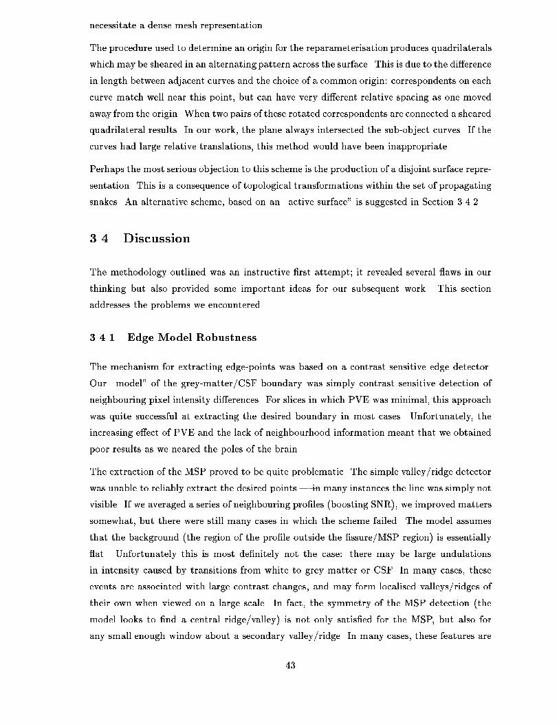
necessitate a dense mesh representation�

The procedure used to determine an origin for the reparameterisation produces quadrilaterals

which may be sheared in an alternating pattern across the surface� This is due to the di�erence

in length between adjacent curves and the choice of a common origin� correspondents on each

curve match well near this point� but can have very di�erent relative spacing as one moved

away from the origin� When two pairs of these rotated correspondents are connected a sheared

quadrilateral results� In our work� the plane always intersected the subobject curves� If the

curves had large relative translations� this method would have been inappropriate�

Perhaps the most serious objection to this scheme is the production of a disjoint surface repre

sentation� This is a consequence of topological transformations within the set of propagating

snakes� An alternative scheme� based on an �active surface is suggested in Section ��

�� Discussion

The methodology outlined was an instructive �rst attempt! it revealed several �aws in our

thinking but also provided some important ideas for our subsequent work� This section

addresses the problems we encountered�

�� Edge Model Robustness

The mechanism for extracting edgepoints was based on a contrast sensitive edge detector�

Our �model of the greymatter�CSF boundary was simply contrast sensitive detection of

neighbouring pixel intensity di�erences� For slices in which PVE was minimal� this approach

was quite successful at extracting the desired boundary in most cases� Unfortunately� the

increasing e�ect of PVE and the lack of neighbourhood information meant that we obtained

poor results as we neared the poles of the brain�

The extraction of the MSP proved to be quite problematic� The simple valley�ridge detector

was unable to reliably extract the desired points � in many instances the line was simply not

visible� If we averaged a series of neighbouring pro�les boosting SNR�� we improved matters

somewhat� but there were still many cases in which the scheme failed� The model assumes

that the background the region of the pro�le outside the �ssure�MSP region� is essentially

�at� Unfortunately this is most de�nitely not the case� there may be large undulations

in intensity caused by transitions from white to grey matter or CSF� In many cases� these

events are associated with large contrast changes� and may form localised valleys�ridges of

their own when viewed on a large scale� In fact� the symmetry of the MSP detection the

model looks to �nd a central ridge�valley� is not only satis�ed for the MSP� but also for

any small enough window about a secondary valley�ridge� In many cases� these features are

��

present in several of the neighbouring pro�les as well� which means that pro�le averaging may

actually accentuate them� Based on these observations� we must conclude that a localised

feature search is completely inappropriate for the detection of the MSP� Furthermore� the

application of a symmetry constraint is problematic within �D images because of patient

machine alignment artifacts� the widths of the hemispheres may be distorted by length

foreshortening�

�� Coping with Topology and Geometry

A fundamental limitation of the above scheme is its inability to deal with topological trans

formations of the snake contours� Attempts could be made to predict how and where such

transitions are likely to occur� but given the sparsity of the data this seems implausible� Al

though we know the topology of the object beforehand from anatomical knowledge� we are

unable to easily mobilize this knowledge in the contourbased segmentation process� For ex

ample� we know that the topology of a brain hemisphere is at the scale we are interested in�

spherical� Of course� simple topology may be associated with �endish geometric complexity

� as the brain illustrates�

The algorithm used to produce a surface from the set of snake curves is crude and places

very speci�c constraints on the type of surface we can construct� Part of the reason for

these limitations arises from our inability to interpolate the missing data� serial sections

of a �D object do not provide a unique representation of that object� This problem has

been studied elsewhere for example �� with some success� However� one has no way of

knowing whether the resulting interpolation will be physiologically meaningful� which is of

paramount importance to us� Furthermore� since our data sets are truncated� the resulting

surface representation will be arti�cially distorted�

If we were to utilise a �D surface for our segmentation we would no longer be required to

implement a separate ��tting step� Better yet� the surface can be made to possess the

correctly topology at the outset� thus overcoming the problems associated with evolving

contour topology� Of course� data truncation would still distort our shape representation�

unless we were able to interpolate the missing surface regions� Such an interpolation would

only be meaningful if it produced a result consistent with brain anatomy� This requires

the inclusion of an anatomical shape constraint in the segmentation process� The use of

implicit shape constraints such as those associated with a Bspline or hyperquadric� would

be insu�cient� since these would not necessarily re�ect the true underlying physiology�

��

�� Conclusion

The use of a �D snakebased segmentation scheme for sparse data was investigated� The

segmentation was based upon Bspline snakes which provide a good framework for the in

clusion of constraints! these constraints are intended to improve robustness by including a

priori knowledge of our problem�

During the course of our investigation it became clear that such a �D segmentation scheme

was fundamentally limited� While there is certainly room for improvement� particularly in

the boundary detection stage� such modi�cations would ultimately fall short of our desire

to quantify complex �D geometric structure� These observations prompted our research into

a �D modelbased methodology� This new approach incorporates aspects of the old line

based� regionspeci�c boundary searches etc� but is based upon a discrete �D model known

as a Simplex Mesh� The bulk of this thesis concerns the development of this new framework

and its validation�

��

Chapter �

Constructing a Shape Template

The selection of an appropriate shape representation is strongly in�uenced by the structures

it is supposed to represent� as well as its intended purpose� For our work� the representation

must be su�ciently general to encompass complex geometry and topology� and �exible enough

to serve as a �shape template� This template will enable us to seek out similar shape

instances within a volumetric image� despite the presence of noise� imaging artifacts and

signi�cant shape variability�

Following from the review and discussion presented in Chapter �� we have rejected parametric

models� with their limited shape resolution� in favour of a dense� discrete mesh representa

tion� Although more powerful continuous parametric descriptions such as Fourier surfaces�

are available� they are subject to certain fundamental limitations� such as the inability to

represent complex topologies� A model capable of representing objects with several �holes

is essential for the segmentation of structures such as the ventricular system� Although the

primary focus of this work is the segmentation and description of objects with spherical topol

ogy cerebral hemispheres�� there is su�cient interest in structures such as the ventricular

system to motivate the development of a more generic segmentation scheme�

As the model complexity increases� the number of parameters required to represent it may

become excessive� This is particularly true for discrete surfaces� in which each vertex repre

sents � additional degrees of freedom� Fortunately� there are methods which can allow one

to reduce the dimensionality of the model� More speci�cally� by examining a set of training

examples segmented surfaces in our case�� it should be possible to construct a representative

model of lower dimensionality by minimising the intraobject redundancy� The reduction

process we utilise � called Principal Components Analysis PCA� � also provides a means

of constraining the permissible shapes the model may assume� This� in turn� stabilises the

segmentation process and provides a framework for the classi�cation of pathological struc

tures�

��

The discrete surface representation we have chosen is the Simplex Mesh �� Within this

framework� it is possible to represent arbitrary topologies� transform from one topology to

another and re�ne the mesh vertex density adaptively�

We begin this chapter with a brief description of the simplex mesh and its properties� The

original mesh segmentation strategy is discussed in Section B�� followed by a review of

possible shape template schemes and an overview of our proposed methodology in Section ��

We then examine the issues which must be addressed if this approach is to be executed

successfully � Section �� and Section �� After presenting the results of our investigations

in Section �� we discuss several issues associated with our particular template scheme �

Section �� before concluding the chapter�

�� The Simplex Mesh

The simplex mesh �� is a discrete surface representation in which each vertex is connected

to � others� Each vertex is associated with a local curvaturelike measure called the �simplex

angle� and may be expressed in terms of its � neighbouring vertices� The mesh formalism

contains a number of strategies to re�ne and update the surface� including a mechanism to

enforce �shape constraints� The reader is referred to Appendix B for additional details�

In its original conception� the simplex mesh was intended as a �D shape description rather

than an active surface for general segmentation� In particular� it was assumed that object

boundaries could be easily and unambiguously identi�ed� Such an assumption was justi�ed

for the �D range data and simple volumetric images used to represent the boundaries of

objects� When one deals with complexmedical images� in which the boundary may be di�cult

to isolate� problems emerge� The use of �D gradient and�or edge thresholded gradient�

images allows the detection of obvious boundaries but fails to locate those that are hidden by

surrounding gradient maxima� Furthermore� the gradient operator is computed in �D� which

may yield poor results for sparse volumetric data�

The segmentation process also requires a high level of interaction to guide the surface to

wards its target� This usually involves the modi�cation of mesh parameters and continuity

constraints� prior to the intialisation of a surface �tting step� The best surface �t of the

available data would be followed by another change of parameters and surface update step�

Repetition of this process eventually leads to a segmentation object description� of the object

from the �D data set�

In order to overcome some of these problems� one may utilise a reference template ��

de�ned through a �shape constraint � Appendix B�� Unfortunately� such a model might

not adequately represent the variability which exists within the given class of shapes� This

��

objection is particularly relevant for biological structures� Although the model will constrain

the mesh to a �reasonable shape this may not be entirely desirable since we have no way of

knowing whether

�� the data which is being detected by our feature search is �good i�e� the actual bound

ary we want�

�� whether the template provides an appropriate representation for this instance of the

shape�

These objections seem to be somewhat justi�ed by the results presented in �� in which a

simplex template of the liver generated through an undisclosed process� was used to segment

that organ from abdominal MRI data� There are signi�cant discrepancies between the model

and the actual data� In certain instances it is not clear whether the model has provided a

reasonable approximation to the organ boundary�

�� Learning Shape Variation

The use of a shape template �� for segmentation provides additional robustness

when we have truncated or noisy data� Missing or noisy boundaries may be interpolated

by the model to provide a compromise solution which should re�ect the true nature of the

underlying shape� If we have a single shape this may be used to de�ne our template� since

we have no interest in representing any other shape instances these would be considered

spurious�� Alternatively� we may allow the template to deform in a speci�ed manner so as to

capture some element of the shape instance which we know a priori�

We require a shape model which can represent a class of objects with high shape variability�

This precludes the use of a shape constraint such as that presented in �� which assumes that

one shape is a suitable representative of an entire class� Furthermore� such an approach does

not place bounds on the permissible shape variation � this facility is useful for classifying

putative abnormalities out of class variation�

One mechanism for the encapsulation of shape variability may be found in Principal Com

ponents Analysis� Within the PCA framework� the variability across a set of vectors which

might represent� for example� vectors of shape descriptors�� is made explicit by the computa

tion of a set of �modes of variation� These modes provide a reduced set of basis vectors on

which similar data may be approximated� The PCA process builds this description by exam

ining a representative �training set of vectors � see Section �� for details� Furthermore�

by noting the extent to which each mode contributes for a given data instance� it is possible

to reject data which are not in good correspondence with the learned variability�

��

For shape processing� the PCA is performed on sets of vectors which provide a description of

the shapes in the training set� If the shapes are represented as Fourier Surfaces� for example�

the coordinates of each shape on the Fourier basis could be used� In general� however�

the shape data is only available through discrete digital sampling and a process has to be

devised to convert this data into a form suitable for analysis� While it may be possible to

�t the discrete mesh data with a continuous parametric form such as a Fourier Surface or

superquadric� this may fail to give a satisfactory result since�

�� the parametric description may be dependent on the spatial orientation of the data�

and

�� the minimisation algorithm utilised by the �tting procedure may be trapped by local

minima� and

�� the associated surface parameterisationmay be inconsistent across the training set� and

�� the parametric form may be limited in topology it can represent� In most cases� only

surfaces with spherical or toroidal topology can be described�

The consistency referred to above concerns the extent to which the surface parameterisation

identi�es �the same point across the training set� This is important for us� since we wish to

gather information about surface structure at corresponding points on each mesh� This topic

will be discussed in Chapter ��

Rather than attempting to resolve these di�culties� we have devised a shape modelling process

based on the direct computation of correspondents� Our de�nition of �correspondent is as

follows� Given two surfaces from a particular class of shapes� which have been aligned as

best as possible� a given point on one surface is considered to be the correspondent of the

point on the other surface which is closest to it� under some sensible distance metric� The

nature of the distance metric� and the manner in which surface alignment can be achieved

are addressed below�

If we are able to associate a point on a given mesh surface with its counterpart on each of

the remaining surfaces� we will have e�ectively parameterised the training set� This �implicit

parameterisation will not provide a means of deducing additional corresponding pairs�� since

there is no underlying continuous surface parameterisation� However� it provides su�cient

infrastructure to support the construction of a shape template�

We propose the following approach for the construction of our model�

Registration The registration step will enable us to identify the surfaces as closely as pos

sible within the chosen class of transformations�� This is a necessary precursor to cor

�Unless the surface is very smooth� in which case we can use interpolation to estimate additional points�

��

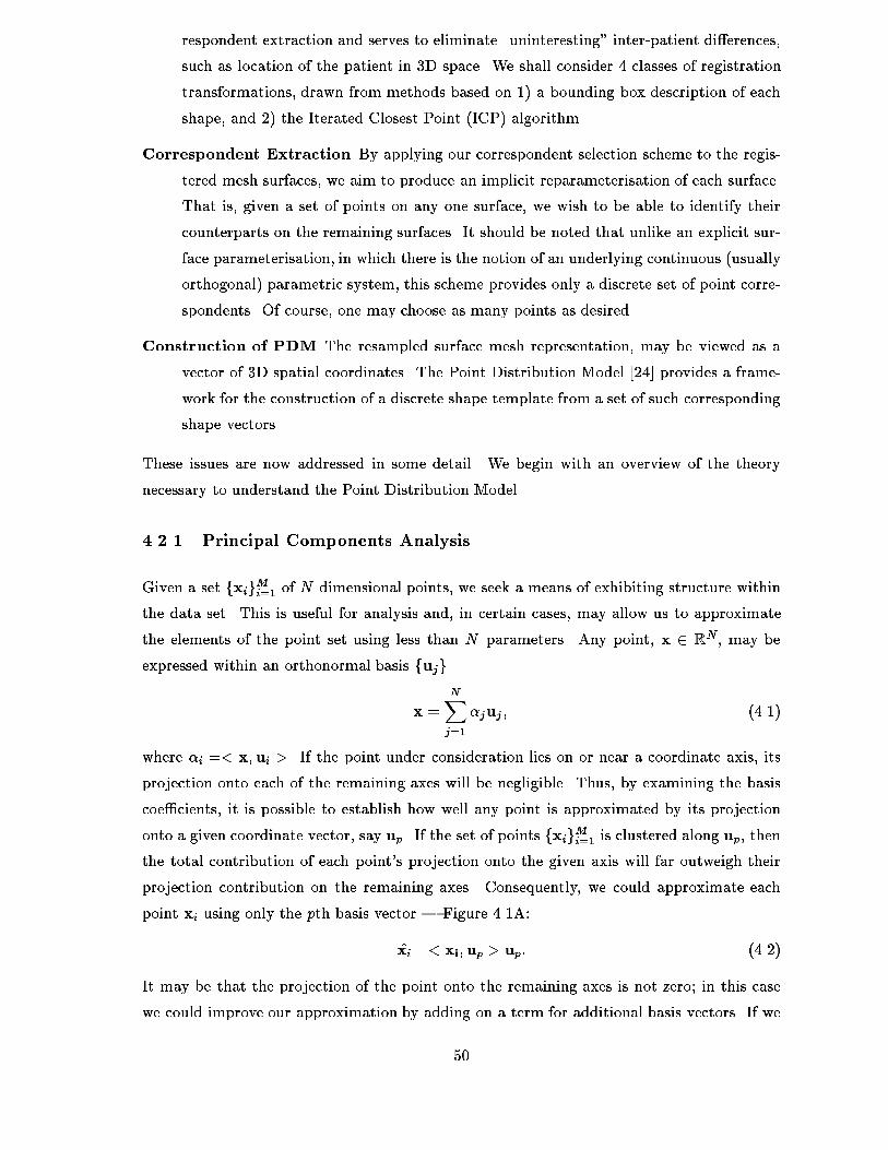
respondent extraction and serves to eliminate �uninteresting interpatient di�erences�

such as location of the patient in �D space� We shall consider � classes of registration

transformations� drawn from methods based on �� a bounding box description of each

shape� and �� the Iterated Closest Point ICP� algorithm�

Correspondent Extraction By applying our correspondent selection scheme to the regis

tered mesh surfaces� we aim to produce an implicit reparameterisation of each surface�

That is� given a set of points on any one surface� we wish to be able to identify their

counterparts on the remaining surfaces� It should be noted that unlike an explicit sur

face parameterisation� in which there is the notion of an underlying continuous usually

orthogonal� parametric system� this scheme provides only a discrete set of point corre

spondents� Of course� one may choose as many points as desired�

Construction of PDM The resampled surface mesh representation� may be viewed as a

vector of �D spatial coordinates� The Point Distribution Model �� provides a frame

work for the construction of a discrete shape template from a set of such corresponding

shape vectors�

These issues are now addressed in some detail� We begin with an overview of the theory

necessary to understand the Point Distribution Model�

�� Principal Components Analysis

Given a set fxigMi�� of N dimensional points� we seek a means of exhibiting structure within

the data set� This is useful for analysis and� in certain cases� may allow us to approximate

the elements of the point set using less than N parameters� Any point� x � RN� may be

expressed within an orthonormal basis fujg

x �NXj��

�juj � ��

where �i �� x�ui �� If the point under consideration lies on or near a coordinate axis� its

projection onto each of the remaining axes will be negligible� Thus� by examining the basis

coe�cients� it is possible to establish how well any point is approximated by its projection

onto a given coordinate vector� say up� If the set of points fxigMi�� is clustered along up� thenthe total contribution of each point�s projection onto the given axis will far outweigh their

projection contribution on the remaining axes� Consequently� we could approximate each

point xi using only the pth basis vector � Figure ��A�

$xi �� xi�up � up� ��

It may be that the projection of the point onto the remaining axes is not zero! in this case

we could improve our approximation by adding on a term for additional basis vectors� If we

��

Approximation

U2

U1

U1’

U2’

Data PointsU1

U2

A B

Figure �� Principal Components For the point clustering shown in A�� each point maybe approximated using only parameter� assuming U and U� are known� This parameteris the projection of the point onto the �principal axis � U in this case� B� For an arbitraryarrangement of points� the PCA process determines the optimal basis which may be usedto approximate the point set� If the points are clustered as shown� then U is the principalaxis� U and U� constitute a orthogonal basis�

associate a cost function

Ck �MXi��

k � xi�uk � k� ��

with the kth coordinate vector� we may re�ne our approximation to the point set by sys

tematically adding the basis vector with the highest score� since this re�ects� on average� the

next most important contributing term in our orthogonal expansion�

We observe two things�

�� We may successively improve our approximation to the point set by adding basis vectors

according to our cost function� and

�� if we only use L basis vectors� where L � N � we may represent each point using only

L parameters assuming that the basis vectors are known�� In other words we have

reduced the dimensionality of the point set from N to L�

Unfortunately� it is unlikely that the point set will be so conveniently arranged� If we blindly

apply this algorithm� we may obtain a very bad estimate unless we retain all the coordinate

vectors� thus gaining nothing� This does not mean that there is no redundancy in the data�

just that it is not obviously exhibited� What we really wish to �nd is a set of orthogonal unit

vectors in our N dimensional space which are such that our cost function Ck is as small as it

can be for each axis�

��

Principal components analysis provides a way of computing these vectors � Figure ��B�

The formulae quoted here� along with a more extensive discussion� may be found in �� For

reasons of economy we shall present only a brief description�

We may express any point� xi� within our N dimensional space on an arbitrary orthonormal

basis� fujg� as

xi �NXj��

�i�juj � ��

To facilitate the derivation below� each point may be alternately represented by $xi

$xi �LXj��

�i�juj NX

j�L��

juj � ��

Of course the two representations are initially equivalent� The fig are the basis coe�cientsfor terms we wish to discard� and are taken to be constant i�e� �i�j � �k�j � j � L � j � N �

We must determine the basis which minimises the residual

EL ��

�

MXn��

kxn � $xnk� � �

�

MXn��

NXj�L��

�n�j � j��

Minimising w�r�t� j we obtain

j ��

M

MXn��

�n�j � ��

If we de�ne the mean x of the point set as

x ��

M

MXi��

xi� ��

we may rewrite the residual as

EL ��

�

MXn��

NXj��

fuTj xn � x�g� ��

��

�

NXj�L��

uTj �uj �

where � is the covariance matrix of the set of vectors� given by

� �Xn

xn � x� xn � x�T � ��

One may show see� for example� �� that the minimum of Equation �� occurs when

�ui � iui� ��

where the ui and i are the eigenvectors and eigenvalues of the covariance matrix�

The residual reduces to EL ��

PNj�L�� j � By discarding the basis� eigenvectors associated

with the smallest N � L eigenvalues� we obtain the optimum description for a speci�ed

dimensionality�

��

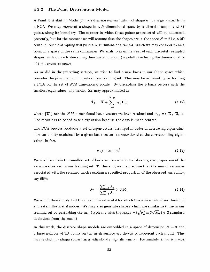
�� The Point Distribution Model

A Point Distribution Model �� is a discrete representation of shape which is generated from

a PCA� We may represent a shape in a N dimensional space by a discrete sampling at M

points along its boundary� The manner in which those points are selected will be addressed

presently� but for the moment we will assume that the shapes are in the space N � � i�e� a �D

contour� Such a sampling will yield a NM dimensional vector� which we may consider to be a

point in a space of the same dimension� We wish to examine a set of such discretely sampled

shapes� with a view to describing their variability and hopefully� reducing the dimensionality

of the parameter space�

As we did in the preceding section� we wish to �nd a new basis in our shape space which

provides the principal components of our training set� This may be achieved by performing

a PCA on the set of NM dimensional points� By discarding the p basis vectors with the

smallest eigenvalues� any model� Xk may approximated as

$Xk � X

N�pXi�i

�k�iUi� ��

where fUig are the NM dimensional basis vectors we have retained and �k�i �� Xk�Ui ��

The mean has to added to the expansion because the data is mean centred�

The PCA process produces a set of eigenvectors� arranged in order of decreasing eigenvalue�

The variability explained by a given basis vector is proportional to the corresponding eigen

value� In fact

�k�i � i � ��i � ��

We wish to retain the smallest set of basis vectors which describes a given proportion of the

variance observed in our training set� To this end� we may require that the sum of variances

associated with the retained modes explain a speci�ed proportion of the observed variability�

say ��%�

T �

Pdn�� nPNn�� n

� ��

We would then simply �nd the maximum value of d for which this sum is below our threshold

and retain the �rst d modes� We may also generate shapes which are similar to those in our

training set by perturbing the �k�i typically with the range �q��k � �

pk! i�e� � standard

deviations from the mean��

In this work� the discrete shape models are embedded in a space of dimension N � � and

a large number of �D points on the mesh surface are chosen to represent each model� This

means that our shape space has a ridiculously high dimension� Fortunately� there is a vast

��

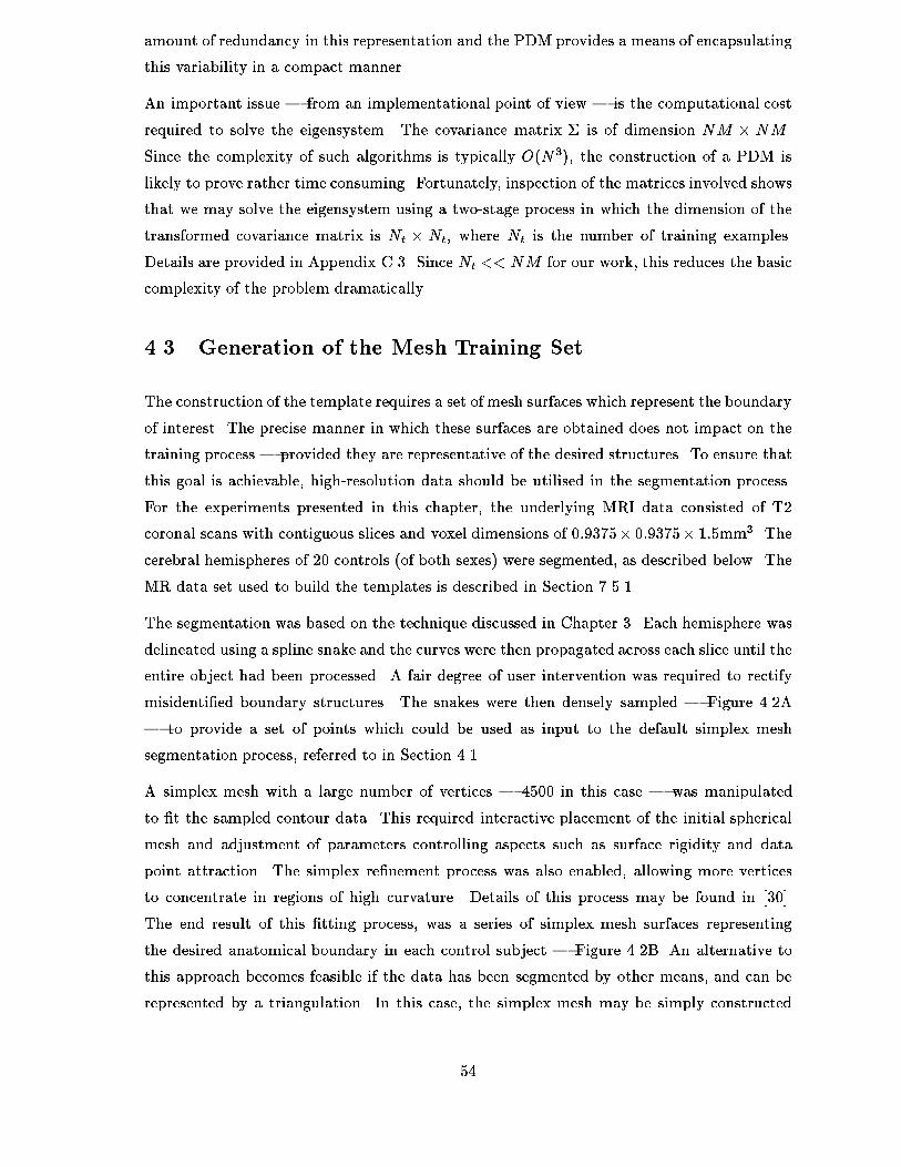
amount of redundancy in this representation and the PDM provides a means of encapsulating

this variability in a compact manner�

An important issue � from an implementational point of view � is the computational cost

required to solve the eigensystem� The covariance matrix & is of dimension NM � NM �

Since the complexity of such algorithms is typically O N�� the construction of a PDM is

likely to prove rather time consuming� Fortunately� inspection of the matrices involved shows

that we may solve the eigensystem using a twostage process in which the dimension of the

transformed covariance matrix is Nt � Nt� where Nt is the number of training examples�

Details are provided in Appendix C�� Since Nt �� NM for our work� this reduces the basic

complexity of the problem dramatically�

�� Generation of the Mesh Training Set

The construction of the template requires a set of mesh surfaces which represent the boundary

of interest� The precise manner in which these surfaces are obtained does not impact on the

training process � provided they are representative of the desired structures� To ensure that

this goal is achievable� highresolution data should be utilised in the segmentation process�

For the experiments presented in this chapter� the underlying MRI data consisted of T�

coronal scans with contiguous slices and voxel dimensions of �� mm�� The

cerebral hemispheres of �� controls of both sexes� were segmented� as described below� The

MR data set used to build the templates is described in Section ��

The segmentation was based on the technique discussed in Chapter �� Each hemisphere was

delineated using a spline snake and the curves were then propagated across each slice until the

entire object had been processed� A fair degree of user intervention was required to rectify

misidenti�ed boundary structures� The snakes were then densely sampled � Figure ��A

� to provide a set of points which could be used as input to the default simplex mesh

segmentation process� referred to in Section ��

A simplex mesh with a large number of vertices � �� in this case � was manipulated

to �t the sampled contour data� This required interactive placement of the initial spherical

mesh and adjustment of parameters controlling aspects such as surface rigidity and data

point attraction� The simplex re�nement process was also enabled� allowing more vertices

to concentrate in regions of high curvature� Details of this process may be found in ��

The end result of this �tting process� was a series of simplex mesh surfaces representing

the desired anatomical boundary in each control subject � Figure ��B� An alternative to

this approach becomes feasible if the data has been segmented by other means� and can be

represented by a triangulation� In this case� the simplex mesh may be simply constructed

��

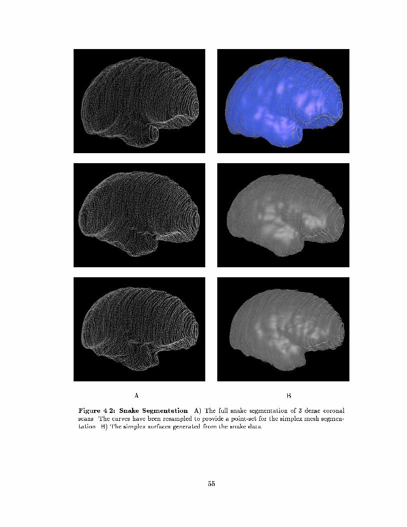
A B

Figure �� Snake Segmentation� A� The full snake segmentation of � dense coronalscans� The curves have been resampled to provide a point�set for the simplex mesh segmen�tation� B� The simplex surfaces generated from the snake data�

��

from the triangulation recall that they are dual representations�� Unfortunately� in this

instance� presegmented data was not available and existing tools had to be used�

The number of vertices in the simplex mesh was chosen to re�ect the nature of the data we

wish to represent� On the one hand� we require a su�ciently large number of vertices to

represent the necessary structure� while on the other� it seems sensible to reduce the com

plexity of the mesh where possible� since it will ultimately serve as a template for extracting

a smoothed approximation to the cerebral surface � which is the best we can hope to do

in the face of data sparsity� Furthermore� since the computational complexity of the active

surface segmentation scheme scales with the number of vertices� it would be unwise to select

an excessively high number� This choice was found to be satisfactory for our requirements

�Figure ��

To ensure the correctness of the segmentations� the snake delineation process was discussed

with neuroanatomists and a consistent procedure developed for the snake segmentation�

The series of images in Figure �� illustrates a number of slices in which these decisions are

re�ected�

Since the hemispheres fuse at the corpus callosum� an arti�cial line had to be extracted in

order to separate the two� The plane of symmetry which cuts the corpus callosum was used

to de�ne this line � Figure ��C�F� When the ventricular spaces were encountered by the

snake� the curve was forced to trace this boundary � Figure ��C� However� the lateral

ventricles were not traced� but bisected by the extension of the midline used to sever the

corpus callosum � Figure ��D�E�

Those parts of the ventricular system which did not intersect the propagating curves were

ignored � Figure ��B�C� When delineating the temporal lobe� the deepest parts of the

sylvian �ssure were ignored� Because the data to be segmented is sparse� a decision was made

to treat the arachnoid as the brain surface� this �cling wrap membrane does not trace deep

sulci and therefore our treatment of the sylvian �ssure and other complex sulcal penetrations

was consistent� The brain stem was excluded� as was the cerebellum � Figure ��E�F�G�

�� Establishing Point Correspondences

In order to construct the PDM� we need to establish corresponding surface points across our

training set� Establishing such relationships is a di�cult task� there is no general algorithm

to parameterise an arbitrary surface� although it is now possible to parameterise speci�c

kinds of surfaces with spherical topology �� However� even with advent of such methods�

additional information is required to pin down the coordinate origin� Furthermore� there

is no guarantee that points which have the same parametric description across patients are

��

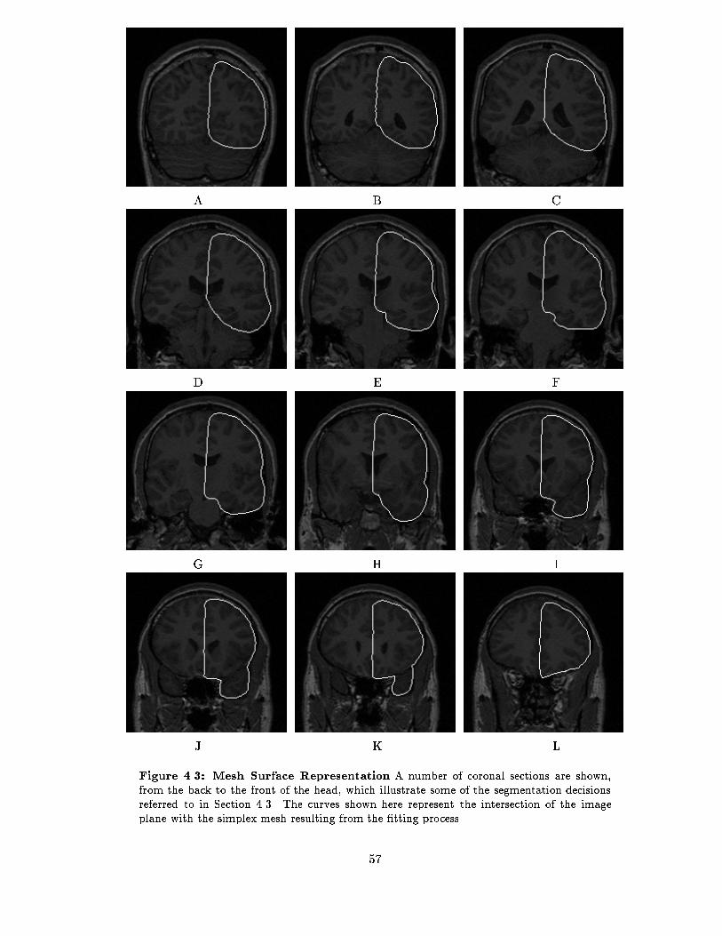
A B C

D E F

G H I

J K L

Figure �� Mesh Surface Representation A number of coronal sections are shown�from the back to the front of the head� which illustrate some of the segmentation decisionsreferred to in Section �� The curves shown here represent the intersection of the imageplane with the simplex mesh resulting from the �tting process�

��

truly the ones we desire�

Rather than attempting to resolve the various problems associated with the determination of

a suitable mesh parameterisation� it seems sensible to adopt an approach which is su�cient for

our requirements� Our primary goal is to establish surface correspondents for both structural

and local greyscale analysis addressed in the next chapter�� If one makes certain assumptions

about the geometric variability across patients� the desired correspondences may be computed

without the need for an explicit parameterisation�

More speci�cally� the following assumptions are made�

Brains are structurally similar across at least� the same sex�

Registration of the data set using global a�ne� transformation will leave signi�cantinterpatient di�erences intact�

We can compute the midsaggital plane MSP��

We can compute the intersection of a ray with the simplex mesh� in practice this meanscomputing the intersection with a triangular mesh generated from the simplex mesh

not necessarily the simplex dual� since this loses vertex segmentation information��

We have complete brain data i�e� no truncations� This is important if we are to construct

a consistent and physiologically meaningful model�

The choice of the registration transformation will have an important impact on the corre

spondent selection scheme� The core idea is simple� if the transformation brings the meshes

into alignment� then choosing the closest point on the target mesh to a given point on the

reference mesh should provide a satisfactory correspondent� Alternatively� the closest point

along the surface normal may be selected� Both of these methods were implemented � the

results are discussed in Section ��

�� Correspondent Extraction

The registration step selects an arbitrary �reference mesh from the training set and attempts

to register each remaining mesh to this surface� Once this has been accomplished a correspon

dent must be established for each point of interest on the reference mesh� In the interests of

simplicity� only mesh vertices were considered� For a speci�ed vertex on the reference mesh�

the correspondent is obtained using�

Normal Sampling A ray from the reference vertex� oriented along the surface normal� is

intersected with the registered target mesh� or�

��

Normal CorrespondentClosest Pt Correspondent

Target

Source

Figure �� Correspondent Selection The correspondents selected by each scheme areshown� Observe that� in general� the selected points may be quite di�erent� unless the surfacesare parallel� In this case the same correspondents will be selected under both schemes� Theorder of the extraction is also important� if the Source and Target surfaces are exchanged� avery di�erent point distribution may arise� unless they are parallel�

Closest Point Sampling For a given reference vertex� the closest mesh point on the regis

tered target mesh is selected� without regard for geometry�

Figure �� shows how the choice of selection scheme a�ects the returned correspondent set�

For parallel surfaces or regions� the two schemes return identical point sets� However� if the

surfaces are very di�erent� there may be a signi�cant di�erence between the two schemes�

Furthermore� if nonparallel surfaces are exchanged� the correspondents may be very di�erent�

These issues will be examined more fully in Section ��

The target mesh is triangulated to provide a surface composed of planar facets � this is

essential for the closest point and ray intersection calculations� The closest point on this

triangulated surface may be found applying the following algorithm�

Algorithm � � �Closest Point on Triangulation�

�� For each vertex� V � on the reference mesh�� For each triangle� Ti� on the target mesh

�� Project the V onto the plane spanned by Ti�� If the point� Pi� lies within this triangle�

CLPT � Pi and we are done! else continue�� Compute the closest point� Pi� on the triangle

boundary�� CLPT � argminPjkV � Pjk�

This calculation may be accelerated by using a spatial indexing scheme to locate a small set

of feasible triangles� and constraining the required calculations to this subset� For surfaces

with extremely complex geometry� such schemes may fail� Fortunately� for the arachnoid�

surfaces we have considered� such an indexing scheme could be usefully employed�

��

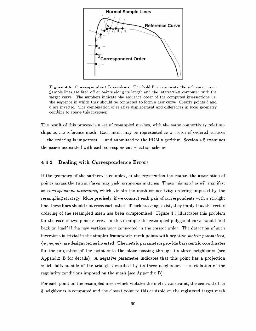
2

3

65

9

Reference Curve

Correspondent Order

Normal Sample Lines

1

4

7 8

Figure �� Correspondent Inversions� The bold line represents the reference curve�Sample lines are �red o� at points along its length and the intersection computed with thetarget curve� The numbers indicate the sequence order of the computed intersections i�e�the sequence in which they should be connected to form a new curve� Clearly points � and� are inverted� The combination of relative displacement and di�erences in local geometrycombine to create this inversion�

The result of this process is a set of resampled meshes� with the same connectivity relation

ships as the reference mesh� Each mesh may be represented as a vector of ordered vertices

� the ordering is important � and submitted to the PDM algorithm� Section �� examines

the issues associated with each correspondent selection scheme�

�� Dealing with Correspondence Errors

If the geometry of the surfaces is complex� or the registration too coarse� the association of

points across the two surfaces may yield erroneous matches� These mismatches will manifest

as correspondent inversions� which violate the mesh connectivity ordering imposed by the

resampling strategy� More precisely� if we connect each pair of correspondents with a straight

line� these lines should not cross each other� If such crossings exist� they imply that the vertex

ordering of the resampled mesh has been compromised� Figure �� illustrates this problem

for the case of two plane curves� In this example the resampled polygonal curve would fold

back on itself if the new vertices were connected in the correct order� The detection of such

inversions is trivial in the simplex framework� mesh points with negative metric parameters�

f�� g� are designated as inverted� The metric parameters provide barycentric coordinatesfor the projection of the point onto the plane passing through its three neighbours see

Appendix B for details�� A negative parameter indicates that this point has a projection

which falls outside of the triangle described by its three neighbours � a violation of the

regularity conditions imposed on the mesh see Appendix B��

For each point on the resampled mesh which violates the metric constraint� the centroid of its

� neighbours is computed and the closest point to this centroid on the registered target mesh

��

4 5

67

21

98

32

1

3

5

67 8

21

3

9

4

76

54

8

32

1

9

Figure �� Example of Vertex Redistribution for a Curve� We start o� by lookingfor correspondences on the target curve� Diagram shows the initial correspondent approx�imation �these were based on normal resampling�� After computing the centroid of eachinverted triple and recomputing the closest point� we get Diagram �� After one more itera�tion we have no more inversions �Diagram �� and each point satis�es the metric constraintfor a ��simplex i�e� every point has a projection onto the line between its � neighbours whichlies between those neighbours�

becomes the new approximation for that correspondent� Figure �� illustrates the idea for a

contour � in the �D case the centroid is computed using the � neighbours of the point under

consideration� The rationale behind this is as follows� because the two surfaces are close

to one another� and similar� most of the correspondences will be correct�� The problematic

points will be surrounded by the patches of good data! we can interpolate this data� subject

to the points lying on the surface and having positive metric constraint� by applying this

�centroidprojection scheme iteratively� This has the e�ect of unknotting foldovers and

providing a best compromise mapping for the correspondents which were initially �snarled�

Algorithm � � �Vertex Redistribution�

�� Repeat until metric constraint is satis�ed forall points or until iteration count is exceeded�� For each point

�� Evaluate f�� g�� If metric constraint violated�� Compute centroid of � neighbours� C�� Find closest point to C on the target mesh

�� Swap newly computed points with old points�� If there are still points which violate the constraint�

�� stabilise the mesh by repeating the above step� but withoutsearching for the closest point any longer�

If the registered meshes are poorly aligned� or the intrinsic geometry too complex� the num

ber of points which violate the metric constraint may be nonzero after a large number of

iterations� This means that the action of projecting onto the target mesh leads to a violation

�At least approximately � it is di�cult to assert that any correspondence is ever truly correct�

��

of the metric constraint prior to the projection� the point � being the centroid of its �

neighbours � has equal� positive metric parameters�� This� in turn� means that the closest

surface point is very di�erent from its neighbours� all of which lie on the target mesh surface�

In this case� we just interpolate the good data� by running the algorithm without requiring

that the problematic points lie on the surface� The full algorithm is presented above�

It should be noted that the application of this algorithm does not guarantee that the �nal

correspondent set will be optimal� this is an almost impossible task without the speci�cation

of additional a priori information� The next section examines the e�ects of the registration

transformation on the selection of the correspondent set�

�� Analysis of Registration Schemes

Before examining the e�cacy of the registration step� the purpose of this process must be

clari�ed� We seek a way of normalising the data so that the only variability contained within

the transformed training set represents the true variability of the class� Since the template

mean shape� involves spatial averaging� maximal alignment of the data is crucial for the

creation of a representative object� The template will serve as the initial shape instance

approximation� Since there is no a priori landmark information� we cannot use a registration

scheme based on such discriminants� the normalisation is intended to allow us to extract

these points�

We wish to learn the structure of the brain� in order to quantify deviation from �normal

ity� To this end� we are prepared to learn redundant information not eliminated by our

normalisation � as long as it does not impact on subsequent segmentation e�orts�

Two classes of transformations have been considered

Bounding Box These global transformations uses the MSP to construct an object centred

coordinate frame � represented as a bounding box � for each mesh� The registration

is performed by mapping the source bounding box onto the reference bounding box�

subject to the speci�ed global mapping rigid or a�ne��

Iterated Closest Points The original ICP formalism �� allowed for the global registra

tion of two point sets� The extensions introduced in �� permit nonrigid registration�

using a volumetric spline technique �� The ICP approach has the advantage of re

quiring no additional information beyond two point sets�

We are not free to choose an arbitrary mapping� The choice of transformation will be con

strained by the assumptions detailed in Section �� In particular� we require that the surfaces

be as close to one another as possible after registration� since this will minimise the incidence

��

of spurious matches�

In an e�ort to quantify the e�ects of the transformation on the selection of the correspondent

set� the following measures have been used�

Inversion Error As the surface registration becomes more accurate� one would expect the

number of correspondent inversions to decrease� In the unlikely� case of perfect registration�

the correspondents are trivially identi�ed as the same point on each registered surface by

means of either correspondent selection strategy � they are identical in this pathological

case�� The initial proportion of correspondents which are inverted� and the rate at which

the inversion correction procedure converges� are taken as indicators of the e�cacy of the

normalisation and the intrinsic correctness of the correspondent set�

Resampling Error Closely allied to the �rst measure is the idea of quantifying the mesh

�resampling error� If one disregards discretisation errors� then a perfectly registered surface

would experience no change of volume or surface area cf� Appendix C� when resampled in

the manner described previously� However� if the correspondent selection process was largely

unsuccessful� the geometry of the resampled surface would vary � perhaps very markedly �

from its original form� By quantifying the di�erence between the prototype and its resampled

version� through volume and surface area changes� as well as surface separation statistics� the

e�ects of normalisation mappings may be compared�

Projection Error By projection error we mean the discrepancy between a surface and its

best approximation under the retained PDM basis� The error is represented through surface

separation statistics mean and standard deviation over the two surfaces�� The purpose

of correspondent selection is to provide the input vectors necessary for the construction of

the PDM� Intuitively� if correct correspondences have been selected� one would expect the

PDM to better encapsulate the true variability within the registered training set� Given the

enormous number of vertices� and the small number of training examples� a reduction in the

number of modes required to represent the chosen level of variability is unlikely�� However� a

more representative PDM should enable one to approximate shape instances within the class

to higher accuracy using the set of retained modes� Consequently� by comparing the original

mesh surface and its best approximation under the PDM� it should be possible to deduce

something about the usefulness of the correspondent selection scheme� Of course� the extent

to which registration aligns the training set will also in�uence these numbers� However�

since the selection of the best registration scheme is part of what we wish to establish� this

�The number of modes cannot exceed the number of training examples� The variability is consequently

forced into these modes and unless there is low variation over the training set� the maximal number of modes

will be required to achieve the best representation�

��

is appropriate� It is worth emphasizing that the di�erence metric must be evaluated after

the surfaces have been registered� The transformation should be the same as that used to

register the training set! the �global information removed by this transformation will not be

re�ected in the PDM�

Qualitative Evaluation The qualitative assessment of the selected correspondents is pro

vided by several graphical renderings� In the �rst� the reference surface and the surface to

be registered are presented from similar views and the selected correspondents are indicated

on each� The second rendering shows the localisation of correspondents across the training

set� by overlaying a random subset of the selected points� One would prefer that the spatial

clustering of the points across patients � for each correspondent � be as centralised as

possible� since this implies that the associated PDM shape space will contain less variability�

This is desirable since the PDM segmentation is less likely to admit spurious shapes�

�� Type I Bounding Box Registration

The de�nition of an objectcentred description is central to this approach� It is assumed that

the MSP has been extracted� This may be accomplished by selecting points lying along the

midsaggital line in a number of slices� and �tting a plane to them using orthogonal regression

� See Chapter �� The MSP normal provides one coordinate axis for the bounding box� By

projecting the mesh points onto the MSP and computing the two principal axes of this point

distribution� a consistent set of coordinate frame may be constructed�

The principal axes of such a point distribution are in�uenced by the arrangement of the

projected points� Clearly this is undesirable as it implies that models which have the same

shape� but which are sampled unevenly� will yield di�erent coordinate frames� We require at

least approximate� invariance to point density at a given resolution � we will use a dense

mesh to minimise discretisation errors��

To overcome this limitation� we compute the convex hull of the planar point set �� and

uniformly sample the returned polygonal contour� This representation� which is invariant to

the internal distribution of the projected points modulo mesh discretisation errors�� is then

subjected to a PCA � Figure �� to obtain the requisite coordinate axes�

Once the reference mesh has been selected� the associated planeconstrained bounding box

is computed and mapped onto the origin� such that the righthanded� coordinate frame is

aligned with that of global coordinate system� For each remaining training example� the

bounding box is computed and the a�ne transformation which maps this bounding box

onto that of the reference is applied to register the source mesh with the reference� The

correspondent selection scheme is then applied� as discussed above�

��

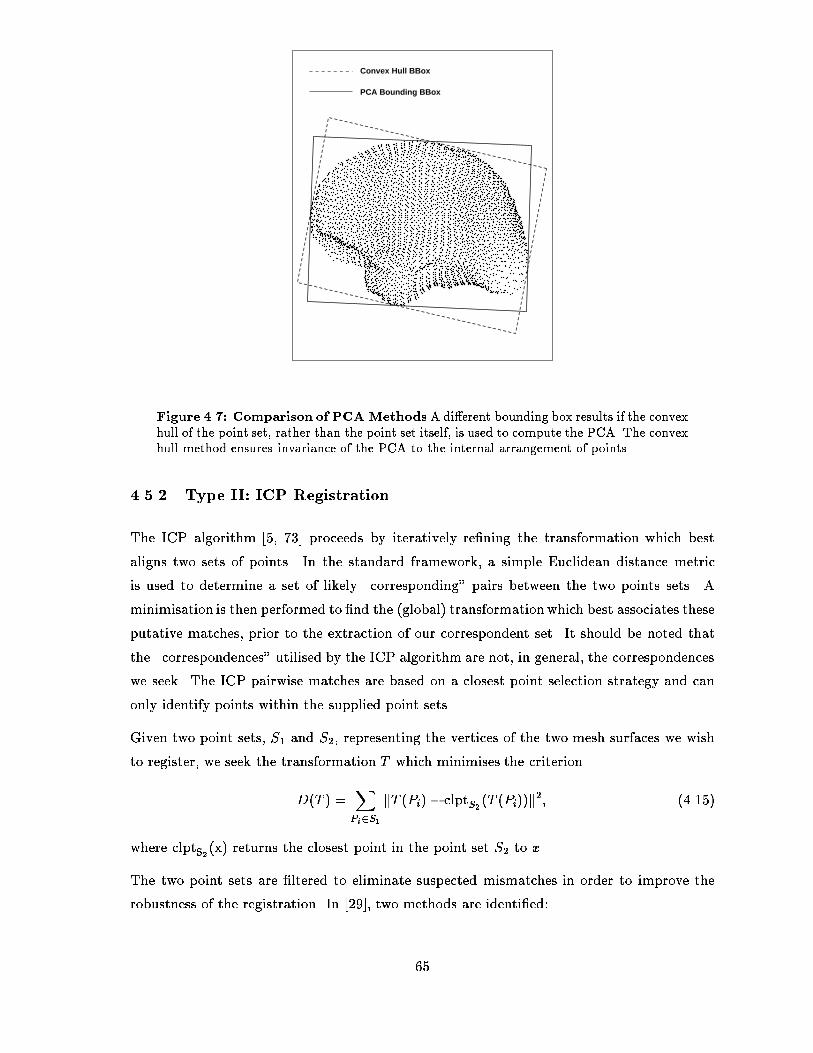
PCA Bounding BBox

Convex Hull BBox

Figure �� Comparison of PCA MethodsA di�erent bounding box results if the convexhull of the point set� rather than the point set itself� is used to compute the PCA� The convexhull method ensures invariance of the PCA to the internal arrangement of points�

�� Type II ICP Registration

The ICP algorithm �� proceeds by iteratively re�ning the transformation which best

aligns two sets of points� In the standard framework� a simple Euclidean distance metric

is used to determine a set of likely �corresponding pairs between the two points sets� A

minimisation is then performed to �nd the global� transformationwhich best associates these

putative matches� prior to the extraction of our correspondent set� It should be noted that

the �correspondences utilised by the ICP algorithm are not� in general� the correspondences

we seek� The ICP pairwise matches are based on a closest point selection strategy and can

only identify points within the supplied point sets�

Given two point sets� S� and S�� representing the vertices of the two mesh surfaces we wish

to register� we seek the transformation T which minimises the criterion

D T � �XPi�S�

kT Pi�� clptS� T Pi��k��

where clptS� x� returns the closest point in the point set S� to x�

The two point sets are �ltered to eliminate suspected mismatches in order to improve the

robustness of the registration� In �� two methods are identi�ed�

��

�� A �xed distance threshold can be used to eliminate patently spurious matches based

on a priori experience��

�� A threshold based on a � statistics is proposed to reject unlikely matches�

The ICP implementation used here is based directly on the work of Feldmar and DeClerck

�� This work introduced notable improvements over the original ICP algorithm� such

as the modi�cation of the �closest point metric to include di�erential information when

available�� The most important modi�cation � for our work � was the introduction of

a nonrigid registration algorithm� By utilising a spacedeforming spline� it is possible to

map one set of points onto another in a smooth� local fashion� For the work presented here�

di�erential information was not utilised�

The A�ne ICP registration is initialised using the best rigid transformation� computed using

the ICP procedure� This is done to ensure stability � the a�ne parameter space is of

su�ciently high dimension that local minima can have a marked impact on the solution� By

bootstrapping the parameter search in this way� a better solution is more likely to emerge�

If spline registration is required� the best a�ne transformation serves as an initialisation�

The volumetric spline is de�ned by a regular grid of �D control points� which directly a�ect

the magnitude of permissible warping�

The spline deformation vector U� V�W �T is de�ned as ��

U x� y� z� �nx��Xi��

ny��Xj��

nz��Xk��

uijkBxi�K x�B

y

j�K y�Bz

k�K z� ��

V x� y� z� �nx��Xi��

ny��Xj��

nz��Xk��

vijkBxi�K x�B

y

j�K y�Bz

k�K z� ��

W x� y� z� �nx��Xi��

ny��Xj��

nz��Xk��

wijkBxi�K x�B

yj�K y�B

zk�K z��

where nx�y�z speci�es the number of control points for each dimension� Bx�y�z

i�Kare the Kth

order Bspline basis functions and u� v� w�Tijk are the control points at index i� j� k�� For this

work� K � �� since cubic Bsplines are employed� The knots are regularly spaced throughout

the volume� A weighted �Tikhonov stabiliser regularising term� given by

E U� �

ZR�

��U

�x�

�

��U

�y�

�

��U

�z�

�

��U

�x�y

�

��U

�x�z

�

��U

�y�z

��

is added to the distance criterion� Equation �� with similar expressions being de�ned for

E V � and E W ��

Once the surfaces have been registered� and correspondents extracted� an �inverse spline

mapping is performed which warps the resampled mesh back on to the result of the best

��

a�ne registration� This is done since� �rstly� the computation of a local spline map is too

costly to implement during segmentation when the model is deployed� and secondly� the

spline transformation has a large number of DOF� This increases the likelihood of running

foul of local minima and reduces the utility of the PDM� which is intended primarily as a

means of constraining the segmentation�

By utilising the best a�ne map to register the meshes� and the best spline map to compute

correspondents� the end result should be better�

�� Results

The results presented in this section are based on the construction of a PDM using �� train

ing examples �� males and � females�� Since only these examples were available� a single

template was generated rather than two genderspeci�c templates� Although there is no easy

criterion to select the number of training examples� quick experiments showed that �� train

ing examples provided a satisfactory variability coverage for the smoothed brain surfaces we

wished to extract� Since the largest sexspeci�c di�erence is one of size� and the a�ne regis

tration used prior to template construction controls for this aspect� the constructed template

is still useful� Furthermore� the primary purpose of this chapter is to evaluate the template

construction procedure� rather than the generation of the best template for a immediate

clinical application�

The qualitative visualisations are presented for the case of the �worst mesh i�e� the one

which was most poorly represented under all our measures of �goodness�

�� Vertex Redistribution

The initial incidence of correspondent inversions varied signi�cantly depending on the choice

of registration scheme � as we had anticipated� Figure �� shows the rate at which the

vertex redistribution corrected the initial inverted correspondents when Normal Sampling

was utilised� This should be compared with Figure �� which shows the details for the case

of Closest point Sampling� Recall that the total number of correspondent pairs is ��

It is immediately obvious that the Closest Point selection performs signi�cantly better than

the Normal Sampling scheme� There are fewer initial inversions� and the rate at which the

vertex redistribution removes inversions is higher�

In some instances� a small set of points remain which must be stabilised using the process

discussed in Section �� This is a consequence of mesh discretisation error� the approxi

mating triangulation cannot adequately represent the underlying surface � implicitly de�ned

��

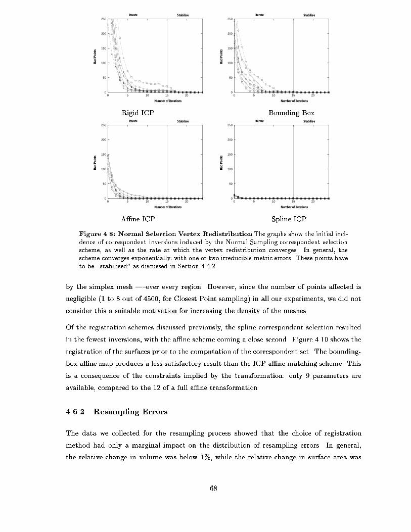
StabiliseIterate

Bad

Poin

ts

Number of Iterations

0

50

100

150

200

250

0 5 10 15 20

StabiliseIterate

Bad

Poin

ts


0

50

100

150

200

250

0 5 10 15 20

Rigid ICP Bounding BoxStabiliseIterate

Bad

Poin

ts


0

50

100

150

200

250

0 5 10 15 20

StabiliseIterate

Bad

Poin

ts


0

50

100

150

200

250

0 5 10 15 20

A�ne ICP Spline ICP

Figure �� Normal Selection Vertex RedistributionThe graphs show the initial inci�dence of correspondent inversions induced by the Normal Sampling correspondent selectionscheme� as well as the rate at which the vertex redistribution converges� In general� thescheme converges exponentially� with one or two irreducible metric errors� These points haveto be �stabilised as discussed in Section ��

by the simplex mesh � over every region� However� since the number of points a�ected is

negligible � to � out of �� for Closest Point sampling� in all our experiments� we did not

consider this a suitable motivation for increasing the density of the meshes�

Of the registration schemes discussed previously� the spline correspondent selection resulted

in the fewest inversions� with the a�ne scheme coming a close second� Figure �� shows the

registration of the surfaces prior to the computation of the correspondent set� The bounding

box a�ne map produces a less satisfactory result than the ICP a�ne matching scheme� This

is a consequence of the constraints implied by the transformation� only � parameters are

available� compared to the �� of a full a�ne transformation�

�� Resampling Errors

The data we collected for the resampling process showed that the choice of registration

method had only a marginal impact on the distribution of resampling errors� In general�

the relative change in volume was below �%� while the relative change in surface area was

��

StabiliseIterate

Bad

Poin

ts


0

50

100

150

200

250

0 5 10 15 20

StabiliseIterate

Bad

Poin

ts


0

50

100

150

200

250

0 5 10 15 20

Rigid ICP Bounding BoxStabiliseIterate

Bad

Poin

ts


0

50

100

150

200

250

0 5 10 15 20

StabiliseIterate

Bad

Poin

ts


0

50

100

150

200

250

0 5 10 15 20


Figure �� Closest Point Vertex RedistributionThe graphs show the initial incidenceof correspondent inversions induced by the Closest point Sampling correspondent selectionscheme� as well as the rate at which the vertex redistribution converges� The vertex redis�tribution converges more smoothly than for the Normal Sampling case� and exhibits fewerinitial inversions�

below �%� The particular correspondent selection scheme was also largely irrelevant� These

observations show that the metric normalisation scheme is quite robust� inversions will be

recti�ed and as a consequence of this process� a fairly uniform and representative discrete

surface will result� It is important to emphasize that the volume and surface area changes

also re�ect the discretisation scale of the resampled mesh�

�� Projection Error

The PDMs associated with the correspondent selection schemes required from �� and ��

modes out of a possible �� the covariance matrix has rank �� to obtain ��% coverage

of variability� This level of coverage is considered to provide an adequate degree of shape

encapsulation ��! additional modes did not noticeably improve shape approximation for

our data�� Figure �� shows the mean and the e�ect of �rst mode of variation for the A�ne

and Rigid PDMs� For the Rigid case� the �rst mode is clearly a global scaling� while in the

A�ne case it a more complex deformation�

��

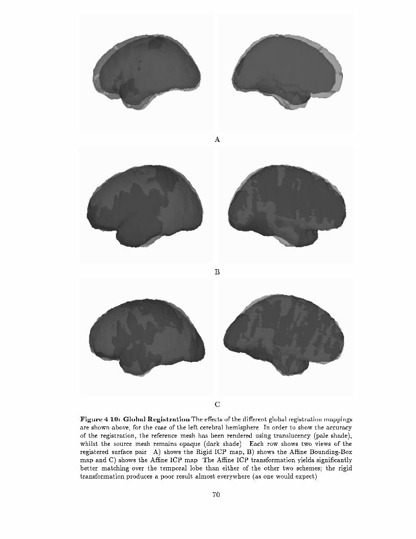
A

B

C

Figure �� Global RegistrationThe e�ects of the di�erent global registration mappingsare shown above� for the case of the left cerebral hemisphere� In order to show the accuracyof the registration� the reference mesh has been rendered using translucency �pale shade��whilst the source mesh remains opaque �dark shade�� Each row shows two views of theregistered surface pair� A� shows the Rigid ICP map� B� shows the A�ne Bounding�Boxmap and C� shows the A�ne ICP map� The A�ne ICP transformation yields signi�cantlybetter matching over the temporal lobe than either of the other two schemes� the rigidtransformation produces a poor result almost everywhere �as one would expect��

��

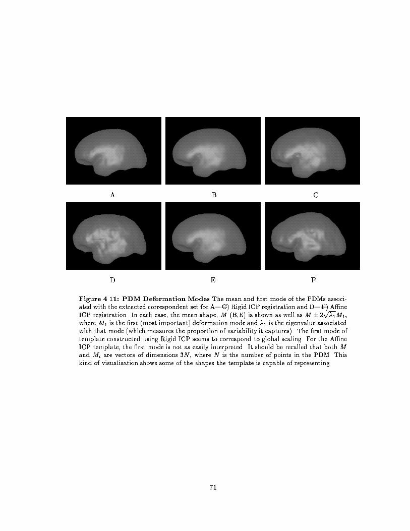
A B C

D E F

Figure �� PDM Deformation Modes The mean and �rst mode of the PDMs associ�ated with the extracted correspondent set for A�C� Rigid ICP registration and D�F� A�neICP registration� In each case� the mean shape� M �B�E� is shown as well as M � �

p��M��

where M� is the �rst �most important� deformation mode and �� is the eigenvalue associatedwith that mode �which measures the proportion of variability it captures�� The �rst mode oftemplate constructed using Rigid ICP seems to correspond to global scaling� For the A�neICP template� the �rst mode is not as easily interpreted� It should be recalled that both M

and Mi are vectors of dimensions �N � where N is the number of points in the PDM� Thiskind of visualisation shows some of the shapes the template is capable of representing�

��

0

0.2

0.4

0.6

0.8

1

0 2 4 6 8 10 12 14 16 18

RigidBBoxAffineSpline

0

0.5

1

1.5

2

2.5

3

3.5

4

0 2 4 6 8 10 12 14 16 18

RigidBBoxAffineSpline

A B

Figure �� Projection Errors A training set of �� mesh surfaces was used to generatea PDM� Fourteen modes explained �� of the variability within this set of shapes� A� showsthe average surface separation �in mm� after approximating each surface in the training setusing the retained modes� B� shows the associated maximum separation for each surface�

The projection error will have a lower bound induced by potentially� poor variability cov

erage� To minimise this e�ect� we have evaluated the projection error only for those mesh

surfaces which formed part of the training set� These measures are aimed at evaluating the ef

fects of the registration transformation and choice of selection scheme� rather than the degree

to which the PDM is able to represent arbitrary shape instances! that issue will be addressed

in a later chapter� With the exception of one example generated from the Rigid PDM� the

relative change in both surface area and volume was well below �%� As Figure ��A shows�

the average surface separation was less than ��mm in all cases� The standard deviation

of this measure was also within ��mm� The maximum separation � Figure ��B � is

the greatest for the Rigid scheme� between ��mm� The remaining schemes produce very

similar results� with maximum separations of ��mm� It is clear from our data that the

Rigid scheme provides the least satisfactory PDM � as one would expect�

�� Qualitative Assessment of Correspondences

The qualitative evaluation of the correspondent set is accomplished by means of a number

of visualisations� which show the selected points on the two surfaces we have chosen� As

we have stated before� no a priori information was utilised to obtain these correspondents�

The results presented here are based on the closest point selection scheme� since this is the

method we intend to use for future correspondent extractions

A randomly selected set of mesh points were extracted on the reference mesh� and the corre

spondents computed on the test surface� A number of views of the computed correspondent

sets are shown in Figure �� and Figure �� It is immediately apparent that a consistent

set of correspondents is extracted for all the proposed transformations� even for the rigid

case� However� the points identi�ed following the A�ne ICP registration appear to provide

��

the most satisfactory results� the relative placement of points is qualitatively correct� The

addition of the Spline deformation does not appear to have improved matters noticeably �

a possible explanation is given in Section ��

Figure �� shows the point clustering of the correspondents over the training set� The e�ect

of the registration is clearly evident� the correspondents extracted after rigid alignment are

more widely scattered� while those extracted after A�ne ICP alignment are comparatively

dense� Interestingly� the Spline correspondent scheme produced a somewhat more di�use

arrangement than the plain A�ne case� This may be due to regularisation problems� as

suggested in Section ��

�� Discussion

On the basis of the quantitative results presented above� the correspondent selection scheme

should be based on the Closest Point sampling strategy� since this ensures a lower number of

correspondent inversions and more rapid convergence of the vertex redistribution procedure�

Intuitively� a lower number of inversions suggests that the manner in which the correspon

dents have been chosen is closer to the underlying reality� Some caution is necessary when

considering this issue� One question in particular requires some thought� is the choice of the

closest point a natural way of selecting a correspondent' If we consider two surfaces such

as those shown in Figure �� the choice of selection method is not so clear cut� When the

source mesh �grows into the target Figure ��A�� the Normally selected correspondents

produced a more natural correspondent selection� Conversely� if the source mesh �shrinks

towards the target � Figure ��B � the Closest Point selection strategy results in a better

correspondent set� Unfortunately� because of its susceptibility to local geometry� the Normal

Selection method is prone to excessive correspondent inversions which must then be recti�ed�

Although the vertex redistribution procedure should regularise the distribution of selected

points� this regularisation depends on the spatial location of the �good i�e� noninverted

correspondents� Clearly� if there is doubt about the validity of these� con�dence in the �nal

correspondent set will be lower�

These troublesome questions can be evaded altogether if the registration succeeds in matching

the surfaces to a su�cient degree� In the ideal case� the surfaces would be superimposed

ensuring that no ambiguity in the choice of correspondents were possible� Of course� this is

unlikely to occur in practice�

By examining both the quantitative and qualitative results presented above� it would seem

that the A�ne ICP mapping provides the most satisfactory global transformation for the

registration step� In this case� the incidence of correspondent inversions is very low less than

��

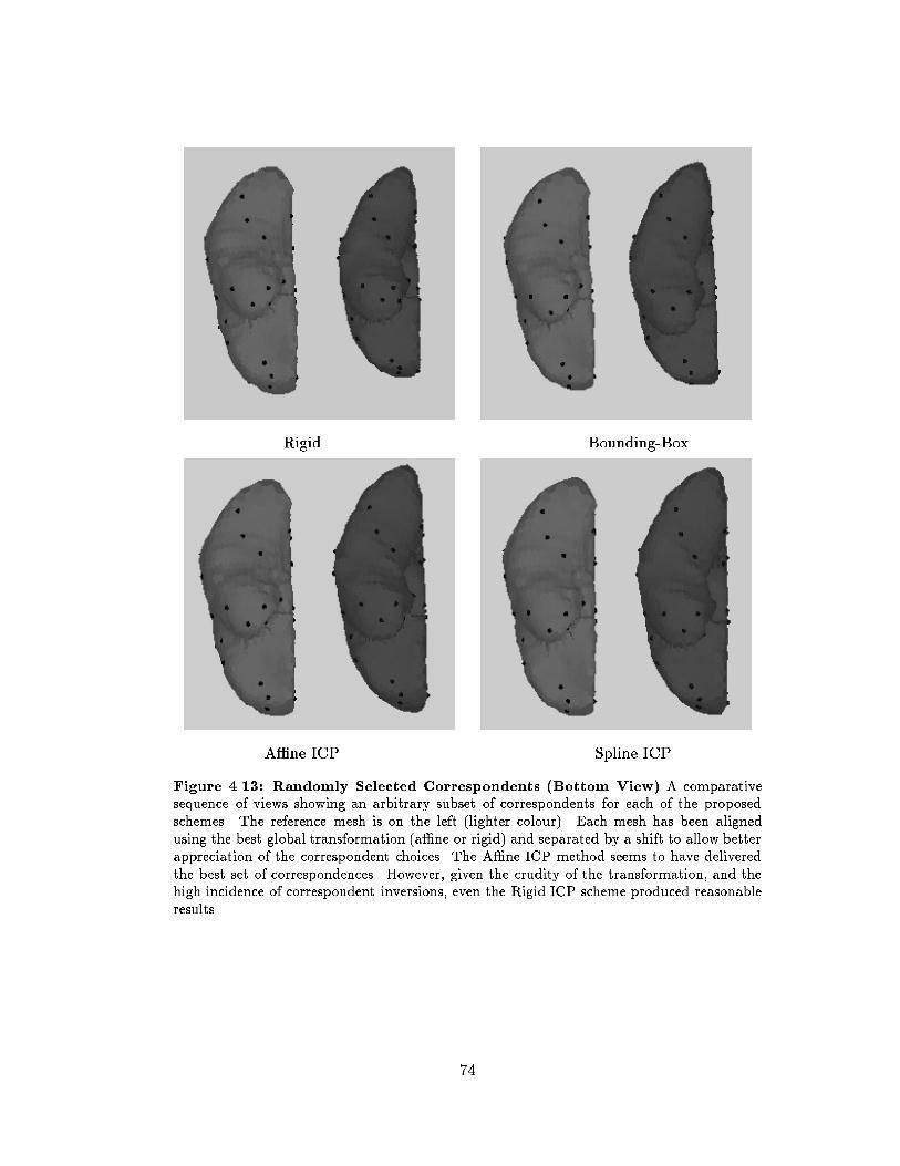
Rigid BoundingBox


Figure �� Randomly Selected Correspondents Bottom View A comparativesequence of views showing an arbitrary subset of correspondents for each of the proposedschemes� The reference mesh is on the left �lighter colour�� Each mesh has been alignedusing the best global transformation �a�ne or rigid� and separated by a shift to allow betterappreciation of the correspondent choices� The A�ne ICP method seems to have deliveredthe best set of correspondences� However� given the crudity of the transformation� and thehigh incidence of correspondent inversions� even the Rigid ICP scheme produced reasonableresults�

��

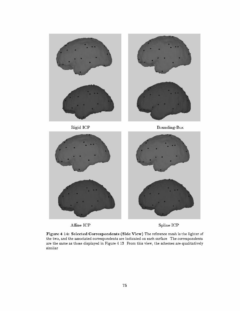
Rigid ICP BoundingBox


Figure �� Selected Correspondents Side View The reference mesh is the lighter ofthe two� and the associated correspondents are indicated on each surface� The correspondentsare the same as those displayed in Figure �� From this view� the schemes are qualitativelysimilar�

��

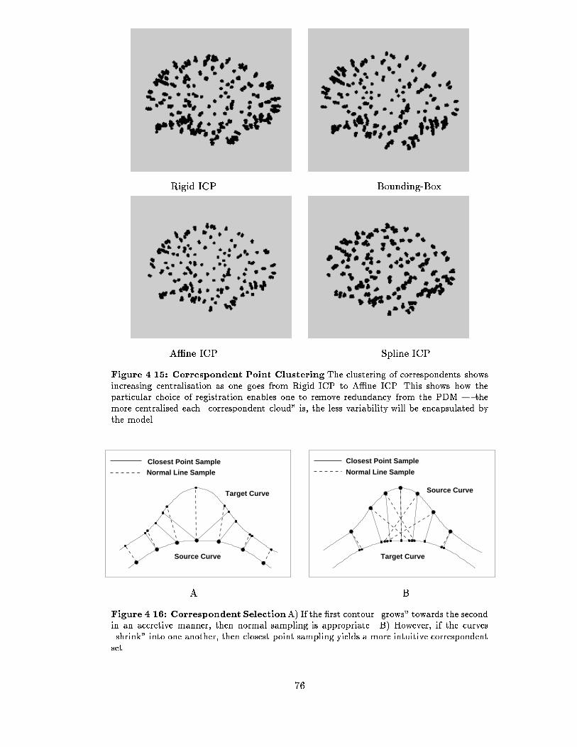
Rigid ICP BoundingBox


Figure �� Correspondent Point Clustering The clustering of correspondents showsincreasing centralisation as one goes from Rigid ICP to A�ne ICP� This shows how theparticular choice of registration enables one to remove redundancy from the PDM � themore centralised each �correspondent cloud is� the less variability will be encapsulated bythe model�

Target Curve

Source Curve

Closest Point Sample

Normal Line Sample

Source Curve

Target Curve

Closest Point Sample

Normal Line Sample

A B

Figure �� Correspondent SelectionA� If the �rst contour �grows towards the secondin an accretive manner� then normal sampling is appropriate� B� However� if the curves�shrink into one another� then closest point sampling yields a more intuitive correspondentset�

��

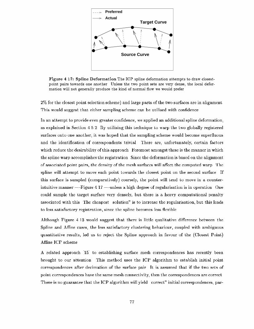
Target Curve

Source Curve

Preferred

Actual

Figure �� Spline Deformation The ICP spline deformation attempts to draw closest�point pairs towards one another� Unless the two point sets are very dense� the local defor�mation will not generally produce the kind of normal �ow we would prefer�

�% for the closest point selection scheme� and large parts of the two surfaces are in alignment�

This would suggest that either sampling scheme can be utilised with con�dence�

In an attempt to provide even greater con�dence� we applied an additional spline deformation�

as explained in Section �� By utilising this technique to warp the two globally registered

surfaces onto one another� it was hoped that the sampling scheme would become super�uous

and the identi�cation of correspondents trivial� There are� unfortunately� certain factors

which reduce the desirability of this approach� Foremost amongst these is the manner in which

the spline warp accomplishes the registration� Since the deformation is based on the alignment

of associated point pairs� the density of the mesh surfaces will a�ect the computed warp� The

spline will attempt to move each point towards the closest point on the second surface� If

this surface is sampled comparatively� coarsely� the point will tend to move in a counter

intuitive manner � Figure �� unless a high degree of regularisation is in operation� One

could sample the target surface very densely� but there is a heavy computational penalty

associated with this� The cheapest �solution is to increase the regularisation� but this leads

to less satisfactory registration� since the spline becomes less �exible�

Although Figure �� would suggest that there is little qualitative di�erence between the

Spline and A�ne cases� the less satisfactory clustering behaviour� coupled with ambiguous

quantitative results� led us to reject the Spline approach in favour of the Closest Point�

A�ne ICP scheme�

A related approach �� to establishing surface mesh correspondences has recently been

brought to our attention� This method uses the ICP algorithm to establish initial point

correspondences after decimation of the surface pair� It is assumed that if the two sets of

point correspondences have the same mesh connectivity� then the correspondences are correct�

There is no guarantee that the ICP algorithmwill yield �correct initial correspondences� par

��

ticularly when the matches must be drawn from decimated vertex sets� The sparse set of

correspondents is interpolated to yield a dense correspondent set� Since no further processing

occurs to validate the initial point selection� this method may yield an unsatisfactory result

when complex geometry is involved�

�� Conclusion

Discussions with neuroanatomists suggest that � at least across each sex � the structure

of the brain is qualitatively similar� Gross di�erences may be removed by a process of

normalisation� whereby the brain surfaces are approximately registered using a particular

family of global transformations� Once such a registration has been accomplished� we are

able to utilise an ad hoc scheme to construct a set of corresponding points on each surface�

without the need for an explicit surface parameterisation or the speci�cation of landmarks�

These correspondences enable us to construct a Point Distribution Model which will be used

to constrain our subsequent segmentation�

Since we are unable to segment deep gyral structure � our data is sparse � the surfaces used

in the training process are taken to represent the arachnoid � a membrane which adheres

to the brain surface� but does not penetrate sulci to any great extent� As a consequence� the

mesh surfaces used in training are comparatively smooth and the correspondent extraction

process quite robust� From both a qualitative and quantitative perspective the use of a global

A�ne transformation� computed using the ICP procedure� produced the most satisfactory

selection of correspondents�

��

Chapter �

Boundary Detection

The reliable detection of points on the brain surface is of fundamental importance to the

mesh segmentation scheme� The accuracy and robustness of the boundary detection scheme

will a�ect the utility and accuracy of the segmentation� Unfortunately� the identi�cation of

these points is not a trivial task� The boundary we seek is associated with complex anatomy�

and may be badly degraded by the sparsity of the data� To overcome these di�culties�

prior information is mobilised at two levels� Firstly� knowledge of the imaging protocol scan

weighting and other acquisition parameters� is exploited and� secondly� anatomical constraints

are imposed� This chapter concerns the development of a boundary detection scheme which

exploits the information at our disposal�

Section �� describes the structure of the brain surface� and explains why the task of boundary

detection is not trivial� In Section �� we outline our basic methodology and propose a num

ber of possible boundary modelling schemes� These schemes are evaluated in Sections ��

and �� The issue of cortical folding is addressed in Section �� Boundary detection results

are presented in Section �� and the chapter concluded in Section ��

�� The Brain Surface Boundary

An idealised crosssection of the brain surface neighbourhood is shown in Figure �� There is

a multitude of membranes� layers and interstices �sinuses� � see� for example� �� Under

most MR protocols� the skin� and skull are easily distinguishable� as is the venous sinus� an

intersticial layer �lled with blood�

The �rst structure one encounters when moving inwards from the skull is the dura mater�

This is composed of an outer layer � which is attached to the inside of the skull � and

an inner layer which surrounds the brain and penetrates the interhemispheric �ssure� The

�By which we mean skin� muscle and fat�

��

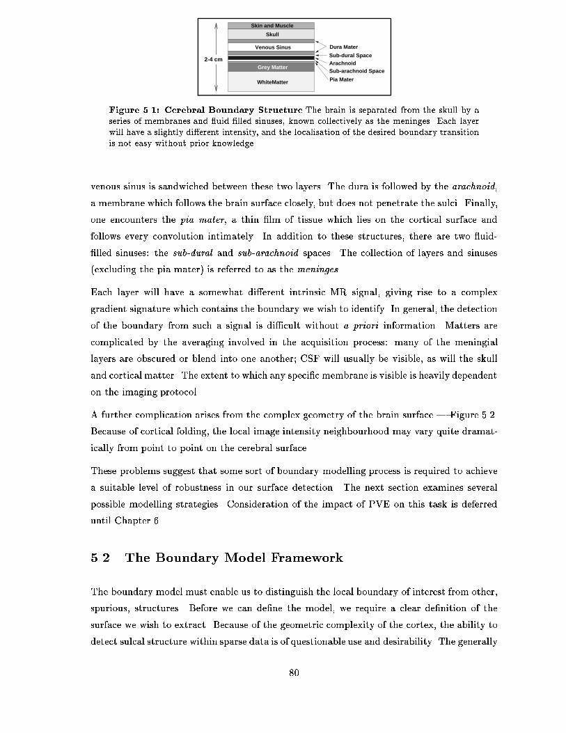
Dura Mater

Pia Mater

2-4 cm

Sub-arachnoid SpaceGrey Matter

Arachnoid

WhiteMatter

Skull

Skin and Muscle

Venous Sinus

Sub-dural Space

Figure �� Cerebral Boundary Structure The brain is separated from the skull by aseries of membranes and �uid �lled sinuses� known collectively as the meninges� Each layerwill have a slightly di�erent intensity� and the localisation of the desired boundary transitionis not easy without prior knowledge�

venous sinus is sandwiched between these two layers� The dura is followed by the arachnoid�

a membrane which follows the brain surface closely� but does not penetrate the sulci� Finally�

one encounters the pia mater� a thin �lm of tissue which lies on the cortical surface and

follows every convolution intimately� In addition to these structures� there are two �uid

�lled sinuses� the sub�dural and sub�arachnoid spaces� The collection of layers and sinuses

excluding the pia mater� is referred to as the meninges�

Each layer will have a somewhat di�erent intrinsic MR signal� giving rise to a complex

gradient signature which contains the boundary we wish to identify� In general� the detection

of the boundary from such a signal is di�cult without a priori information� Matters are

complicated by the averaging involved in the acquisition process� many of the meningial

layers are obscured or blend into one another! CSF will usually be visible� as will the skull

and cortical matter� The extent to which any speci�c membrane is visible is heavily dependent

on the imaging protocol�

A further complication arises from the complex geometry of the brain surface � Figure ��

Because of cortical folding� the local image intensity neighbourhood may vary quite dramat

ically from point to point on the cerebral surface�

These problems suggest that some sort of boundary modelling process is required to achieve

a suitable level of robustness in our surface detection� The next section examines several

possible modelling strategies� Consideration of the impact of PVE on this task is deferred

until Chapter ��

�� The Boundary Model Framework

The boundary model must enable us to distinguish the local boundary of interest from other�

spurious� structures� Before we can de�ne the model� we require a clear de�nition of the

surface we wish to extract� Because of the geometric complexity of the cortex� the ability to

detect sulcal structure within sparse data is of questionable use and desirability� The generally

��

White Matter

GreyMatter

Arachnoid

Intensity Profiles

Figure �� Cortical Folding The cortex has a very convoluted structure which ensuresthat the large�scale boundary structure varies dramatically across the cerebral surface� The�gure shows � di�erent grey level intensity pro�les sampled normally to the cerebral surface�Note how the complex sulcal penetrations induce marked di�erences in the intensity pro�les�all of which are nominally representing the same collection of surface points�

poor correlation between sulci over neighbouring sparse slices poses di�culties for the surface

�tting procedure� which must interpolate the available data smoothly� For this reason� we

have decided that the arachnoid is the most representative boundary for the description of the

brain surface� Unfortunately� in many instances it is not visible� blending into surrounding

meningial structures� The model should aim to extract as close an approximation to the

arachnoid as possible! at the very least� it should not permit edge points to be detected

within sulci� Furthermore� since the contrast in an image di�ers signi�cantly from protocol

to protocol� the model representation should be loosely coupled to the imaging protocol� to

facilitate the construction of a generic approach�

�� Model Input Data

At the core of our proposed modelling process is a �D vector of intensity values� extracted by

sampling the volumetric image along a ray emanating from the mesh surface� Each vector

speci�es a �D signal which may be processed by standard methods to detect boundary�edge

transitions� The choice of a �D intensity neighbourhood� rather than a �D or �D neighbour

hood� was motivated primarily by computational economy� Such a strategy was also used for

our preliminary work with snakes � Chapter ��

In the sparse framework� these intensity samples are constrained to lie within the individual

image slices which comprise the �D volumetric image� Within the slice� the intensity sampling

errors are signi�cantly smaller when compared with those which arise when full �D line

sampling is performed� By only using data within each image slice� we provide more accurate

input information for our models�

��

During the boundary detection phase� intensity vectors for selected points on the surface

mesh are extracted� The model is applied to each vector� yielding a set of �D boundary

points which are used to update the model � see Chapter ��

�� The Models

We have implemented three kinds of models�

M� Edge Heuristics The simplest approach � a set of heuristics for processing gradient

and grey scale information is provided which attempts to locate the desired gradient

from those present� Only relative gradient strengths and greylevel comparisons are

used�

M� PCA Models During the mesh template training phase� �D grey level information

from each corresponding point is used to build an average surfacenormal intensity

pro�le with associated modes of variation� This is a variant of the �D scheme imple

mented by Cootes et al �� In this scenario� grey level information is used directly�

which means that intensity normalisation must be applied to the images� Furthermore�

separate models are required for each standard protocol T�� T� and PD��

M� Speci�ed Models Using knowledge of anatomy� we may construct a model or a set

of them� which encapsulate the variability we know to be present� The model is rep

resented as a piecewise constant curve� in which the individual segments have variable

length� Because the characteristic grey level signature of a given boundary type varies

with protocol� a separate set of models may be required for each�

The requirement that sulci be ignored during boundary detection will not be directly incorpo

rated into the boundary model� Instead� a scheme will be derived whereby boundary points

which deviate dramatically from points known to lie on the �arachnoid or our approxima

tion to this surface� will be rejected� This issue will be fully addressed in Section ��

�� Edge Heuristics

This scheme is ideally suited to Zonebased boundary detection� the heuristics required are

manually speci�ed� If one were required to produce a di�erent set of heuristics for each node�

the amount of work required would be excessive�

The model is built as follows�

�� A number of representative �D greylevel pro�les are subjected to a �D Canny edge

detector of a speci�ed scale�

��

�� The resulting set of gradient maxima locations and magnitudes� fxi� G xi�g� providesa disjoint decomposition of each intensity pro�le! the intensity values are averaged over

each pair xi� xi�� to provide an average intensity for each edge separated interval�

fgig

�� The set fxi� G xi�� gig is then examined for obvious algebraic relationships� For example� if we had a step edge going from bright to dark� we could say that� given a

gradient edge point� candidate� if the pixels to the left were on average� brighter than

those to the right� that this point matched our model� If we have a series of alternating

gradients� then we may mobilise the gradient information to �lter out spurious edge

point candidates�

We only constructed two models� a model for the cortexCSF boundary and one for the

midsaggital line� The MSP detector was initially taken to be a valley detector� since this

is an intuitive representation for this feature� Unfortunately� in many instances this line is

NOT visible recall Figure �� from Chapter �� Furthermore� once the brain hemispheres

fuse� the line will vanish�

The cortexCSF model represents a bright region followed by a dark region� followed by a

bright region� corresponding to cortical tissue� CSF and skull on a T�weighted scan� The

� largest gradients are selected output from a �D Canny edge detector�� and if the edge

contrast is correct� and the average grey level characteristics are consistent� a given edge

point is �agged as the boundary point� To compensate for the possible exclusion of the skull

from the intensity sample� a rule is coded which will enable a step edge representing the

cortexCSF boundary� to be detected� The gradient must be of the appropriate polarity� and

should be the largest present� Some examples are shown in Figure ��

There are numerous problems with this simple approach� In particular� the scale at which

edges should be detected is not at all clear� As the imaging plane intersects the tissue

boundary at an increasingly acute angle� cosine foreshortening comes into play� and the

edges are stretched or compressed� A scale appropriate to the �equatorial region is likely

to be highly inappropriate for the �polar region of the cerebral hemispheres� Furthermore�

localised intensity inhomogeneities can cause pathological gradient maxima which confound

any set of simple heuristics� There is also a de�nite dependence on the imaging protocol�

since the heuristics require knowledge of edge contrast and average grey level characteristics�

Finally� the lack of a suitable means to detect points on the midsaggital lines is undesir

able� the brain often possesses a notable curvature of this supposedly planar structure� To

accurately represent the data� we need to detect at least some of these points�

��

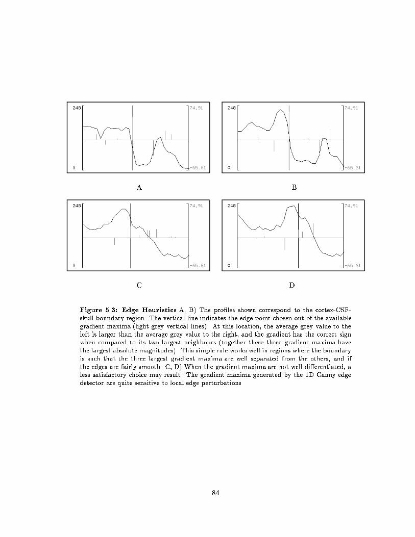
A B

C D

Figure �� Edge Heuristics A� B� The pro�les shown correspond to the cortex�CSF�skull boundary region� The vertical line indicates the edge point chosen out of the availablegradient maxima �light grey vertical lines�� At this location� the average grey value to theleft is larger than the average grey value to the right� and the gradient has the correct signwhen compared to its two largest neighbours �together these three gradient maxima havethe largest absolute magnitudes�� This simple rule works well in regions where the boundaryis such that the three largest gradient maxima are well separated from the others� and ifthe edges are fairly smooth� C� D� When the gradient maxima are not well di�erentiated� aless satisfactory choice may result� The gradient maxima generated by the D Canny edgedetector are quite sensitive to local edge perturbations�

��

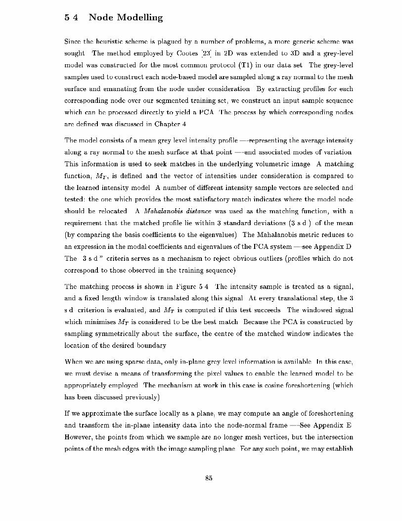
�� Node Modelling

Since the heuristic scheme is plagued by a number of problems� a more generic scheme was

sought� The method employed by Cootes �� in �D was extended to �D and a greylevel

model was constructed for the most common protocol T�� in our data set� The greylevel

samples used to construct each nodebased model are sampled along a ray normal to the mesh

surface and emanating from the node under consideration� By extracting pro�les for each

corresponding node over our segmented training set� we construct an input sample sequence

which can be processed directly to yield a PCA� The process by which corresponding nodes

are de�ned was discussed in Chapter ��

The model consists of a mean grey level intensity pro�le � representing the average intensity

along a ray normal to the mesh surface at that point � and associated modes of variation�

This information is used to seek matches in the underlying volumetric image� A matching

function� MT � is de�ned and the vector of intensities under consideration is compared to

the learned intensity model� A number of di�erent intensity sample vectors are selected and

tested� the one which provides the most satisfactory match indicates where the model node

should be relocated� A Mahalanobis distance was used as the matching function� with a

requirement that the matched pro�le lie within � standard deviations � s�d�� of the mean

by comparing the basis coe�cients to the eigenvalues�� The Mahalanobis metric reduces to

an expression in the modal coe�cients and eigenvalues of the PCA system� see Appendix D�

The �� s�d� criteria serves as a mechanism to reject obvious outliers pro�les which do not

correspond to those observed in the training sequence��

The matching process is shown in Figure �� The intensity sample is treated as a signal�

and a �xed length window is translated along this signal� At every translational step� the �

s�d� criterion is evaluated� and MT is computed if this test succeeds� The windowed signal

which minimisesMT is considered to be the best match� Because the PCA is constructed by

sampling symmetrically about the surface� the centre of the matched window indicates the

location of the desired boundary�

When we are using sparse data� only inplane grey level information is available� In this case�

we must devise a means of transforming the pixel values to enable the learned model to be

appropriately employed� The mechanism at work in this case is cosine foreshortening which

has been discussed previously��

If we approximate the surface locally as a plane� we may compute an angle of foreshortening

and transform the inplane intensity data into the nodenormal frame � See Appendix E�

However� the points from which we sample are no longer mesh vertices� but the intersection

points of the mesh edges with the image sampling plane� For any such point� we may establish

��

Window

T = t1 T = t2 T = t3

Accept

TTM (t1) > M (t2)Mean

Accept Reject

Figure �� Matching Under the Mahalanobis Criterion The intensity sample maybe viewed as a signal� We de�ne a window� with a sample size equivalent to that used tode�ne the PCA vectors� and evaluate MT �� at various translational o�sets along the signal�If the windowed signal is further than � s�d� from the PCA mean� it is rejected immediately�Otherwise� the Mahalanobis matching function is evaluated and the windowed signal whichminimises this distance is chosen �located at T � t� in this example�� The centre of thismatched window indicates the location of the target boundary�

the closest mesh node� and hence the model which is most appropriate for matching local

intensity data� By applying the algorithm stated above to the transformed data� we may �nd

the best inplane translation for each boundary point� The set of these planar translations

may be utilised in the model update process discussed in Chapter ��

The node modelling process did not yield very satisfactory models� As Figure �� shows�

the averaging of pro�les from a number of training pro�les leads to unrepresentative grey

level models� This is particularly evident in Figure ��B� which shows the mean greylevel

model generated from pro�les extracted near the top of the brain� Since PVE is maximal

in this region� and the model is to be mobilised to clean up the data� this is a particularly

unsatisfactory �nding� Examination of this �gure shows several problems with this automated

process�

intensity curves may be translated w�r�t� one another�

some curves appear to represent very di�erent structures�

As we stated in Section �� even if precise correspondences are available� the complexity of the

gyral structure near the brain surface can give rise to very di�erent intensity pro�les� It is clear

from these graphs� that the correspondences are not precise� since some of the curves seem

to be approximately related by a translation� Unfortunately� one cannot simply �register

these curves� since there will be nonlinear warping in addition to this linear transformation

tissue widths can vary signi�cantly across patients��

��

0

20

40

60

80

100

120

140

160

180

200

0 5 10 15 20 25 30 35 40

Data 1Data 2Data 3Data 4

0

20

40

60

80

100

120

140

160

180

200

0 5 10 15 20 25 30 35 40

Mean Profile

A B

Figure �� Pro�le PCA A� Because of local di�erences in brain geometry� the intensitypro�les extracted at points considered to be correspondents can vary considerably� Theboundaries delimiting the cerebral and inner skull surfaces have been bracketed for two ofthe pro�les� The approximate location of the edges are indicated by solid circles� Observethat the curves cannot be properly registered using simple translation� B� The mean pro�leis only vaguely suggestive of the underlying anatomy and is signi�cantly reduced in intensity�

As a consequence� the grey level PCA can admit solutions which bear little relation to the

underlying anatomy � Figure �� It seems that the only suitable means by which we may

impose a sensible grey level model is to mobilise our knowledge of boundary anatomy to

directly specify the models of interest�

�� Specifying a model

Before describing the process by which these models may be de�ned and applied� we will sum

marise a number of important properties concerning the boundary structure we are interested

in�

�� The idealised intensity pro�le sampled along a normal ray emanating from the cortical

surface yields a piecewise constant curve in the absence of noise� imaging artifacts and

PVE��

�� The widths of the individual piecewise constant segments which represent various

tissues��uids� will� in general� exhibit very signi�cant inter and intra subject variability�

They are dynamic entities�

�� In general� the relative intensity relationships between tissue types will be preserved

for a given protocol� For example� in a T� weighted scan� grey matter will always be

brighter than CSF�

�� The ordering of tissues is generally preserved� Provided the intensity pro�le is sampled

consistently for example� along the normal ray pointing away from the brain surface��

one will always �nd that cortex precedes CSF� which precedes skull etc� Note that the

��

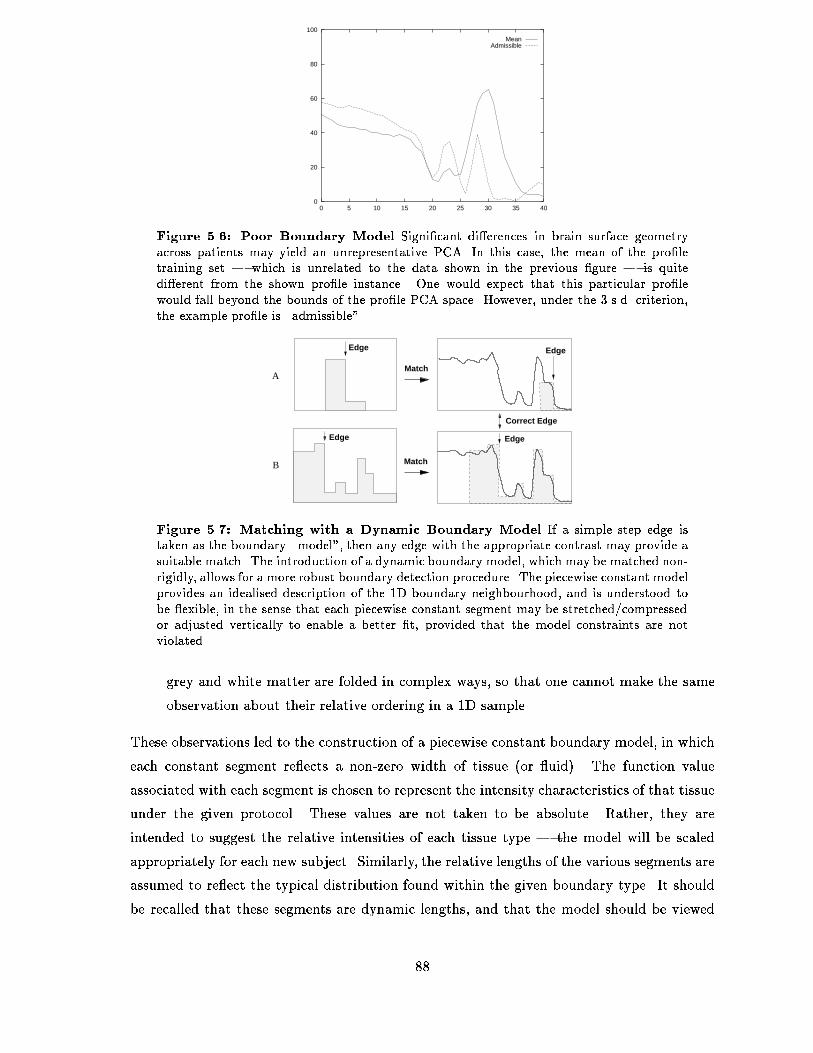
0

20

40

60

80

100

0 5 10 15 20 25 30 35 40

MeanAdmissible

Figure �� Poor Boundary Model Signi�cant di�erences in brain surface geometryacross patients may yield an unrepresentative PCA� In this case� the mean of the pro�letraining set � which is unrelated to the data shown in the previous �gure � is quitedi�erent from the shown pro�le instance� One would expect that this particular pro�lewould fall beyond the bounds of the pro�le PCA space� However� under the � s�d� criterion�the example pro�le is �admissible �

Match

Match

B

Edge

A

Correct Edge

Edge

Edge

Edge

Figure �� Matching with a Dynamic Boundary Model If a simple step edge istaken as the boundary �model � then any edge with the appropriate contrast may provide asuitable match� The introduction of a dynamic boundary model� which may be matched non�rigidly� allows for a more robust boundary detection procedure� The piecewise constant modelprovides an idealised description of the D boundary neighbourhood� and is understood tobe �exible� in the sense that each piecewise constant segment may be stretched�compressedor adjusted vertically to enable a better �t� provided that the model constraints are notviolated�

grey and white matter are folded in complex ways� so that one cannot make the same

observation about their relative ordering in a �D sample�

These observations led to the construction of a piecewise constant boundary model� in which

each constant segment re�ects a nonzero width of tissue or �uid�� The function value

associated with each segment is chosen to represent the intensity characteristics of that tissue

under the given protocol� These values are not taken to be absolute� Rather� they are

intended to suggest the relative intensities of each tissue type � the model will be scaled

appropriately for each new subject� Similarly� the relative lengths of the various segments are

assumed to re�ect the typical distribution found within the given boundary type� It should

be recalled that these segments are dynamic lengths� and that the model should be viewed

��

as a dynamic entity which is suggestive of the boundary to be modelled� Such a model is

shown in Figure �� which also shows how the richness of the model description serves to

disambiguate potential mismatches�

�� Model Construction and Representation

The models are built using the following procedure�

�� The number of distinct boundary models is �rst established� Knowledge of anatomy

can be used in the case of medical data� or a number of boundary intensity pro�les

can be examined from each image� Intensity pro�les with the the same arrangement

of tissue bands� but having di�erent tissue widths� are described by a single model�

The number of tissue bands can be estimated visually the intensities should be near

uniform��

�� For each boundary model� the intensity relationships between each piecewise segment

are noted� If one tissue is always brighter than another� the relative heights of the two

segments will re�ect this relationship� Under the currents scheme if two segments have

multiple intensity relationships� a new model will be created for each permutation�

�� The intensity relationships and segment widths are directly re�ected in the shape of

the piecewise constant curve representing the boundary model� The model does not

encode absolute width or intensity� however� During boundary detection� the model

will be vertically scaled� whilst the segment width are considered to be mutable�

Each model is stored as a sequence of numbers� representing the intensity values of the

piecewise constant segments� The sample length of each piecewise segment which naturally

consists of identical numbers� is proportional to the width of the corresponding tissue band�

During matching� these segments are allowed to expand or contract� so the number of samples

may be deduced by looking at a representative intensity pro�le� The edge of interest is

unambiguously speci�ed by storing the index of the appropiate edge transition for example�

the transition between white and grey matter segments�� Constraints on the extent to which

the models may deform are introduced in Section ��

�� Matching the Model to Data

Given a candidate intensity pro�le� the model must be deployed to detect the boundary of

interest� The model is stored as a discrete� piecewise constant pro�le� with a label which

identi�es the transition which corresponds to the boundary edge of interest� If the model

represented a boundary with �xed widths� then a simple correlation or least squares error

criterion could be used to �t the model to the curve after appropriate scaling�� The location

��

Translate

Selected Edge Selected Edge

Figure �� Simple Translation In the simplest case� the boundary of interest would havea static pro�le� and a simple matching scheme based on model translation would su�ce� Sincethe edge of interest within the boundary model is known� the location of the appropriateedge transition within the matched boundary model can be used to infer the location of theedge within the signal�

of the tagged edge transition would then identify the best approximation to the edge point

within the �D intensity array � Figure ��

Of course� this situation is unlikely to occur in practice� as we have already observed� To

provide the level of �exibility we require� a local �tting scheme is required � one which

will maintain the required segment ordering and intensity relationships� This is not an easy

undertaking� there is no obvious minimisation procedure which will yield the best piecewise

constant �t to an arbitrary curve� It is tempting to generalise the case of simple translation

into a full a�ne transformation�W �

W M x�� M �x T � ��

where T is the translation of the model� M � and � is a scaling constant� This would permit

a uniform compression or dilation of the model� in addition to a translation� While this

would provide an additional degree of freedom� the transformationW imposes an unnatural

constraint on the �exibility of the tissue segments�

This objection suggests that a nonlinear matching algorithm is required� Conceptually� the

nonlinearity we seek should permit complete freedom for model deformation� subject to our

constraints� namely�

�� The piecewise constant form of the model must be preserved�

�� The tissue�segment ordering must be preserved�

�� The intensity interrelationships between segments must be preserved�

Our matching strategy is built around a coarseto�ne approach� The model is �rst decom

posed into a sequence of local �model elements� representing �prominent structures within

the piecewise constant pro�le� These are �xed groups of adjacent segments which will be

��

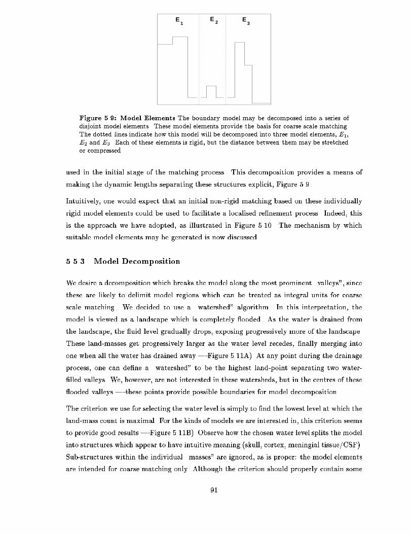
32E E E1

Figure �� Model Elements The boundary model may be decomposed into a series ofdisjoint model elements� These model elements provide the basis for coarse scale matching�The dotted lines indicate how this model will be decomposed into three model elements� E��E� and E�� Each of these elements is rigid� but the distance between them may be stretchedor compressed�

used in the initial stage of the matching process� This decomposition provides a means of

making the dynamic lengths separating these structures explicit� Figure ��

Intuitively� one would expect that an initial nonrigid matching based on these individually

rigid model elements could be used to facilitate a localised re�nement process� Indeed� this

is the approach we have adopted� as illustrated in Figure �� The mechanism by which

suitable model elements may be generated is now discussed�

�� Model Decomposition

We desire a decomposition which breaks the model along the most prominent �valleys� since

these are likely to delimit model regions which can be treated as integral units for coarse

scale matching� We decided to use a �watershed algorithm� In this interpretation� the

model is viewed as a landscape which is completely �ooded� As the water is drained from

the landscape� the �uid level gradually drops� exposing progressively more of the landscape�

These landmasses get progressively larger as the water level recedes� �nally merging into

one when all the water has drained away � Figure ��A�� At any point during the drainage

process� one can de�ne a �watershed to be the highest landpoint separating two water

�lled valleys� We� however� are not interested in these watersheds� but in the centres of these

�ooded valleys � these points provide possible boundaries for model decomposition�

The criterion we use for selecting the water level is simply to �nd the lowest level at which the

landmass count is maximal� For the kinds of models we are interested in� this criterion seems

to provide good results � Figure ��B�� Observe how the chosen water level splits the model

into structures which appear to have intuitive meaning skull� cortex� meningial tissue�CSF��

Substructures within the individual �masses are ignored� as is proper� the model elements

are intended for coarse matching only� Although the criterion should properly contain some

��

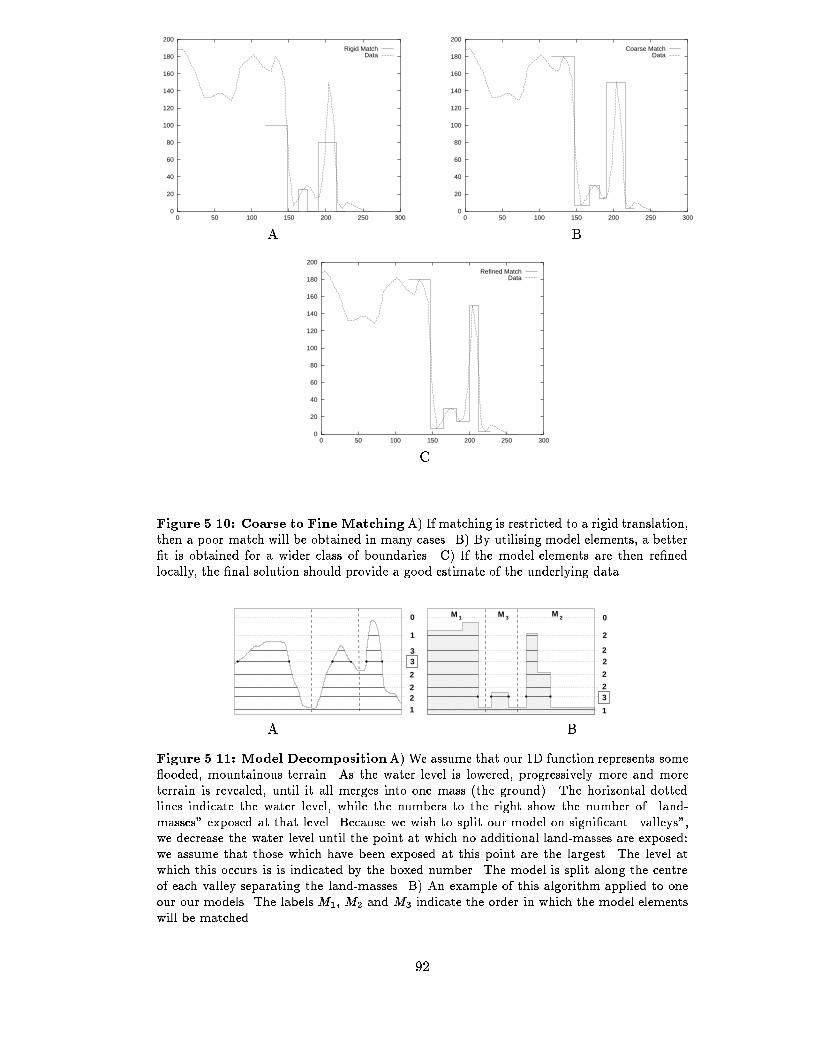
0

20

40

60

80

100

120

140

160

180

200

0 50 100 150 200 250 300

Rigid MatchData

0

20

40

60

80

100

120

140

160

180

200

0 50 100 150 200 250 300

Coarse MatchData

A B

0

20

40

60

80

100

120

140

160

180

200

0 50 100 150 200 250 300

Refined MatchData

C

Figure �� Coarse to Fine MatchingA� If matching is restricted to a rigid translation�then a poor match will be obtained in many cases� B� By utilising model elements� a better�t is obtained for a wider class of boundaries� C� If the model elements are then re�nedlocally� the �nal solution should provide a good estimate of the underlying data�

1

32

2

2

M 2M3M1

2

2

0

33

2

2

0

11

2

A B

Figure �� Model DecompositionA� We assume that our D function represents some�ooded� mountainous terrain� As the water level is lowered� progressively more and moreterrain is revealed� until it all merges into one mass �the ground�� The horizontal dottedlines indicate the water level� while the numbers to the right show the number of �land�masses exposed at that level� Because we wish to split our model on signi�cant �valleys �we decrease the water level until the point at which no additional land�masses are exposed�we assume that those which have been exposed at this point are the largest� The level atwhich this occurs is is indicated by the boxed number� The model is split along the centreof each valley separating the land�masses� B� An example of this algorithm applied to oneour our models� The labels M�� M� and M� indicate the order in which the model elementswill be matched�

��

notion of scale� to avoid the detection of small valleys� it is well suited to the simple piecewise

constant pro�les we wish to decompose�

�� Coarse Matching

The coarse scale matching process is itself based on a coarseto�ne strategy� the largest

model elements are matched �rst� We have adopted a very simple metric to quantify model

element size� the area bounded by the piecewise constant curve within each element� see

Figure ��B�� Furthermore� the matching process must maintain the spatial ordering of the

model elements� since anything else is anatomically incorrect� The matching energy is taken

to be the sum of squared di�erences� Other di�erence measures� such a crosscorrelation�

could also have been employed� Under this di�erence measure� the �tting process for each

model element reduces to �nding the �D translation which yields the smallest residual� As

stated above� the elements are matched from largest to smallest and the spatial ordering

imposed by the original model is enforced�

The algorithm is as follows�

Algorithm � � �Coarse Matching�

�� Smooth the input data signal� S � fsigi�� N �with a unit variance Gaussian� to yield SG�

�� Scale the model data� M � so that the model maximumcoincides with the that of SG�

�� Decompose the model using the watershed algorithm� toyield ordered model elements� fE�� EPg�

�� For each Ei� compute the model size� and thus de�nethe order in which the Ei will be matched�

�� For each Ei� in size order�� If any models have been matched to the left� set

the leftmost translation limit to the right edge ofthe relevant matched model� L� otherwise set L � ��

�� If any models have been matched to the right� setthe rightmost translation limit to the right edge ofthe relevant matched model� R� otherwise set R � N �

�� If the new model element is too small to �t within �L�R��terminate matching�

�� For each translational position in �L�R�� Evaluate the sum of squared di�erences residual�

�� Select the translation position corresponding to the minimumof the residual set�

Statement �� in the algorithm raises a very important issue� the role of the initial model

scale� While the model is �exible� the size of the model elements imposes a lower limit

on scale of the features which may be matched� Coarse level matching only permits the

��

space between model elements to expand or contract! the model elements themselves are

rigid� Consequently� if two matched structures are very close to one another� then small scale

detail may be missed between them� This problem may be overcome by de�ning a model in

which the a�ected structure is appropriately scaled down� The whole issue of model size is

intimately related to the issue of discretisation� and will be discussed fully in Section ��

Some examples of this kind of matching are shown in Figure ��

Observe that although the overall match is improved� when compared to simple translation�

the edges do not generally �t the data very well�

�� Local Matching

If the coarse matching has succeeded� then both the edge estimates and the piecewise con

stant �t need to be locally re�ned� The edge re�nement process is accomplished by locally

translating the relevant step edge and noting the variation in the sum of squared di�erences�

residual� We shall assume that an �edge point is located at the centre of a nonideal edge�

This assumption is reasonable except in the presence of large PVE � in this case� as we shall

show� the edge point may be perturbed from this central location� It should be noted that�

under this de�nition� the edge location might not correspond to a point of in�exion on the

local curve�

We justify this assumption on the following grounds�

Simplicity If one only has a discrete �D signal� and a rough idea of the height of the di�use

edge� then the edge point may be estimated by translating a step edge of the appropriate

height and contrast along the signal and noting where the residual between the signal

and the step achieves its minimum�

Foreshortening Eects In the absence of noise or imaging artifacts� a piecewise constant

boundary pro�le will retain its ideal edges� except when the underlying tissue is sam

pled obliquely relative to the surface normal� This results in to �rst order� cosine

foreshortening� which linearly scales the distances between the edges� If one assumes

that the edges are slightly imperfect� and could be approximated by a very steep ramp�

then it would be reasonable to take the edge point as being in the centre of this ramp�

The ramp would also be subject to linear separation� but the edge point would retain its

central position� These foreshortening e�ects are clearly visible in much of the intensity

pro�les we have to process� A discussion of foreshortening may be found in Appendix E�

With these comments in mind� we shall de�ne the optimal edge location as one at which the

sum of squared di�erences between a local step edge of size �R samples� and the underly

ing signal achieves its minimum� The size of R will be addressed in Section �� When

��

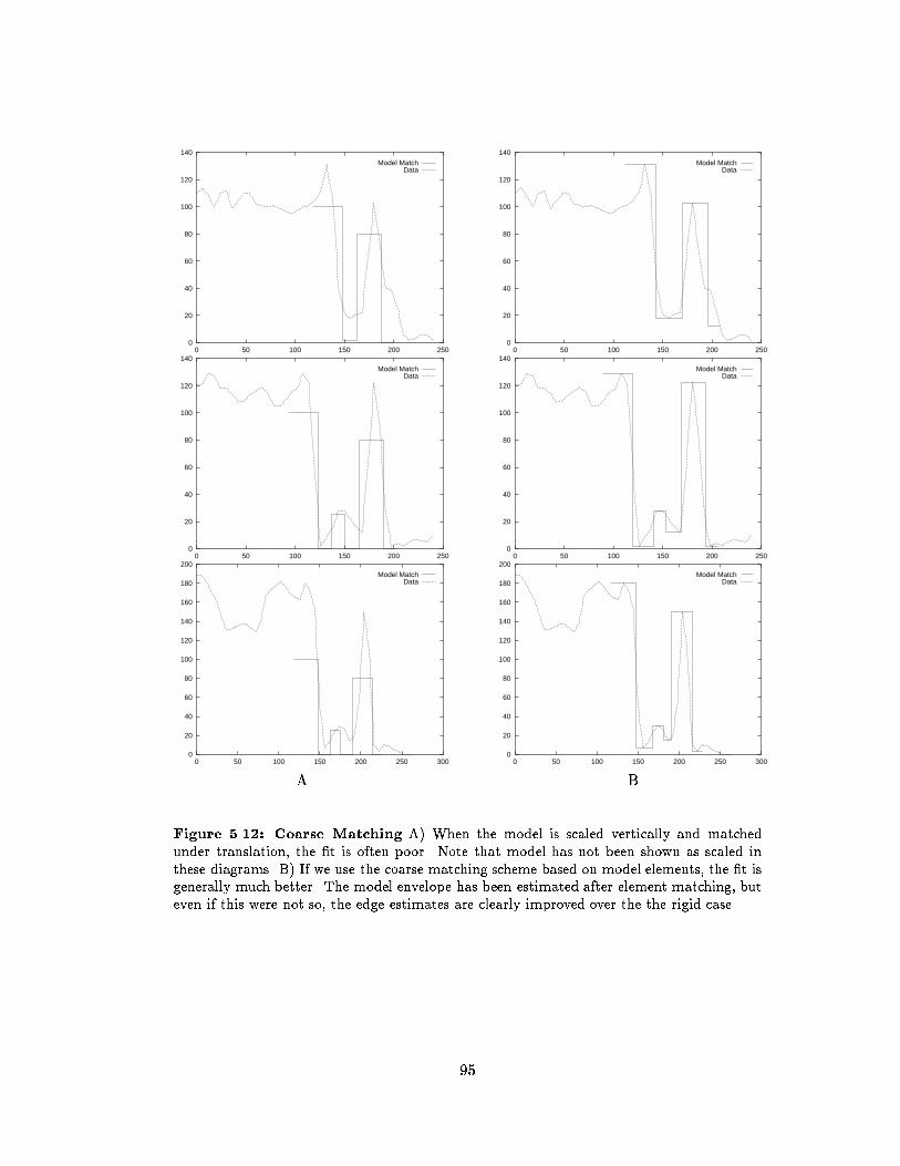
0

20

40

60

80

100

120

140

0 50 100 150 200 250

Model MatchData

0

20

40

60

80

100

120

140

0 50 100 150 200 250

Model MatchData

0

20

40

60

80

100

120

140

0 50 100 150 200 250

Model MatchData

0

20

40

60

80

100

120

140

0 50 100 150 200 250

Model MatchData

0

20

40

60

80

100

120

140

160

180

200

0 50 100 150 200 250 300

Model MatchData

0

20

40

60

80

100

120

140

160

180

200

0 50 100 150 200 250 300

Model MatchData

A B

Figure �� Coarse Matching A� When the model is scaled vertically and matchedunder translation� the �t is often poor� Note that model has not been shown as scaled inthese diagrams� B� If we use the coarse matching scheme based on model elements� the �t isgenerally much better� The model envelope has been estimated after element matching� buteven if this were not so� the edge estimates are clearly improved over the the rigid case�

��

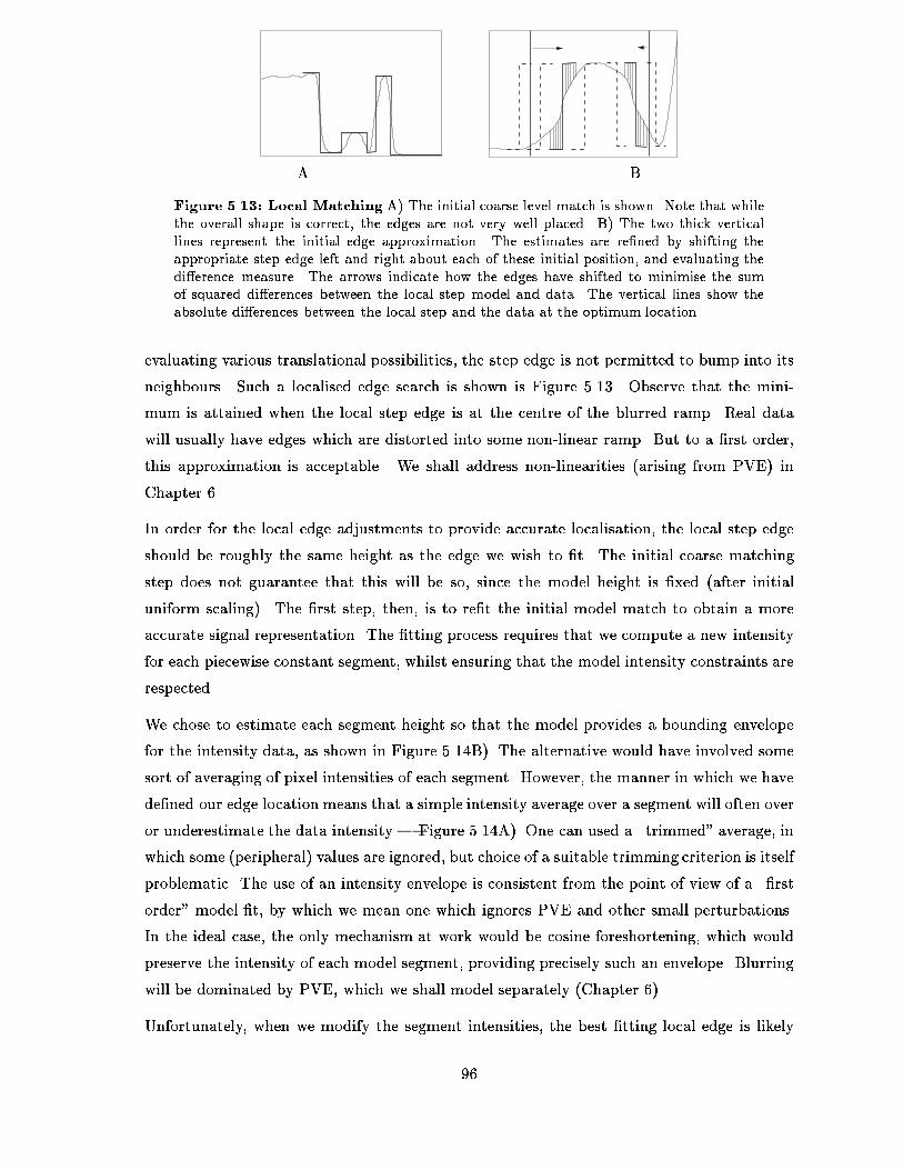
A B

Figure �� Local Matching A� The initial coarse level match is shown� Note that whilethe overall shape is correct� the edges are not very well placed� B� The two thick verticallines represent the initial edge approximation� The estimates are re�ned by shifting theappropriate step edge left and right about each of these initial position� and evaluating thedi�erence measure� The arrows indicate how the edges have shifted to minimise the sumof squared di�erences between the local step model and data� The vertical lines show theabsolute di�erences between the local step and the data at the optimum location�

evaluating various translational possibilities� the step edge is not permitted to bump into its

neighbours� Such a localised edge search is shown is Figure �� Observe that the mini

mum is attained when the local step edge is at the centre of the blurred ramp� Real data

will usually have edges which are distorted into some nonlinear ramp� But to a �rst order�

this approximation is acceptable� We shall address nonlinearities arising from PVE� in

Chapter ��

In order for the local edge adjustments to provide accurate localisation� the local step edge

should be roughly the same height as the edge we wish to �t� The initial coarse matching

step does not guarantee that this will be so� since the model height is �xed after initial

uniform scaling�� The �rst step� then� is to re�t the initial model match to obtain a more

accurate signal representation� The �tting process requires that we compute a new intensity

for each piecewise constant segment� whilst ensuring that the model intensity constraints are

respected�

We chose to estimate each segment height so that the model provides a bounding envelope

for the intensity data� as shown in Figure ��B�� The alternative would have involved some

sort of averaging of pixel intensities of each segment� However� the manner in which we have

de�ned our edge location means that a simple intensity average over a segment will often over

or underestimate the data intensity � Figure ��A�� One can used a �trimmed average� in

which some peripheral� values are ignored� but choice of a suitable trimming criterion is itself

problematic� The use of an intensity envelope is consistent from the point of view of a ��rst

order model �t� by which we mean one which ignores PVE and other small perturbations�

In the ideal case� the only mechanism at work would be cosine foreshortening� which would

preserve the intensity of each model segment� providing precisely such an envelope� Blurring

will be dominated by PVE� which we shall model separately Chapter ��

Unfortunately� when we modify the segment intensities� the best �tting local edge is likely

��

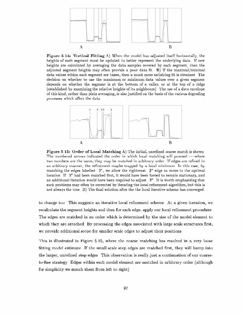
A B

Figure �� Vertical Fitting A� When the model has adjusted itself horizontally� theheights of each segment must be updated to better represent the underlying data� If newheights are calculated by averaging the data samples covered by each segment� then theadjusted segment heights may often provide a poor data �t� B� If the maximal�minimaldata values within each segment are taken� then a much more satisfying �t is obtained� Thedecision on whether to use the maximum or minimum data values over a given segmentdepends on whether the segment is at the bottom of a valley� or at the top of a ridge�established by examining the relative heights of its neighbours�� The use of a data envelopeof this kind� rather than plain averaging� is also justi�ed on the basis of the various degradingprocesses which a�ect the data�

1 2233

A B

Figure �� Order of Local Matching A� The initial� unre�ned coarse match is shown�The numbered arrows indicated the order in which local matching will proceed � wheretwo numbers are the same� they may be matched in arbitrary order� If edges are re�ned inan arbitrary manner� the re�nement maybe trapped by a local minimum� In this case� bymatching the edges labelled �� we allow the rightmost �� edge to move to the optimallocation� If �� had been matched �rst� it would have been forced to remain stationary� andan additional iteration would have been required to adjust �� It is worth emphasizing thatsuch problems may often be corrected by iterating the local re�nement algorithm� but this isnot always the true� B� The �nal solution after the the local iterative scheme has converged�

to change too� This suggests an iterative local re�nement scheme� At a given iteration� we

recalculate the segment heights and then for each edge� apply our local re�nement procedure�

The edges are matched in an order which is determined by the size of the model element to

which they are attached� By processing the edges associated with large scale structures �rst�

we provide additional scope for smaller scale edges to adjust their positions�

This is illustrated in Figure �� where the coarse matching has resulted in a very loose

�tting model estimate� If the small scale step edges are matched �rst� they will bump into

the larger� unre�ned step edges� This observation is really just a continuation of our coarse

to�ne strategy� Edges within each model element are matched in arbitrary order although

for simplicity we match them from left to right��

��

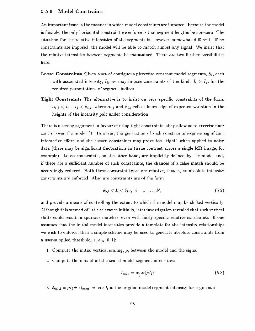
�� Model Constraints

An important issue is the manner in which model constraints are imposed� Because the model

is �exible� the only horizontal constraint we enforce is that segment lengths be nonzero� The

situation for the relative intensities of the segments is� however� somewhat di�erent� If no

constraints are imposed� the model will be able to match almost any signal� We insist that

the relative intensities between segments be maintained� There are two further possibilities

here�

Loose Constraints Given a set of contiguous piecewise constant model segments� Si� each

with associated intensity� Ii� we may impose constraints of the kind� Ii � Ij � for the

required permutations of segment indices�

Tight Constraints The alternative is to insist on very speci�c constraints of the form�

�i�j � Ii � Ij � i�j � where �i�j and i�j re�ect knowledge of expected variation in the

heights of the intensity pair under consideration�

There is a strong argument in favour of using tight constraints� they allow us to exercise �ner

control over the model �t� However� the generation of such constraints requires signi�cant

interactive e�ort� and the chosen constraints may prove too �tight when applied to noisy

data there may be signi�cant �uctuations in tissue contrast across a single MR image� for

example�� Loose constraints� on the other hand� are implicitly de�ned by the model and�

if there are a su�cient number of such constraints� the chances of a false match should be

accordingly reduced� Both these constraint types are relative� that is� no absolute intensity

constraints are enforced� Absolute constraints are of the form

��i � Ii � ��i� i � �� N� ��

and provide a means of controlling the extent to which the model may be shifted vertically�

Although this seemed of little relevance initially� later investigation revealed that such vertical

shifts could result in spurious matches� even with fairly speci�c relative constraints� If one

assumes that the initial model intensities provide a template for the intensity relationships

we wish to enforce� then a simple scheme may be used to generate absolute constraints from

a usersupplied threshold� ��

�� Compute the initial vertical scaling� �� between the model and the signal�

�� Compute the max of all the scaled model segment intensities�

Imax � maxif�Iig� ��

�� i � �Ii �Imax� where Ii is the original model segment intensity for segment i�

��

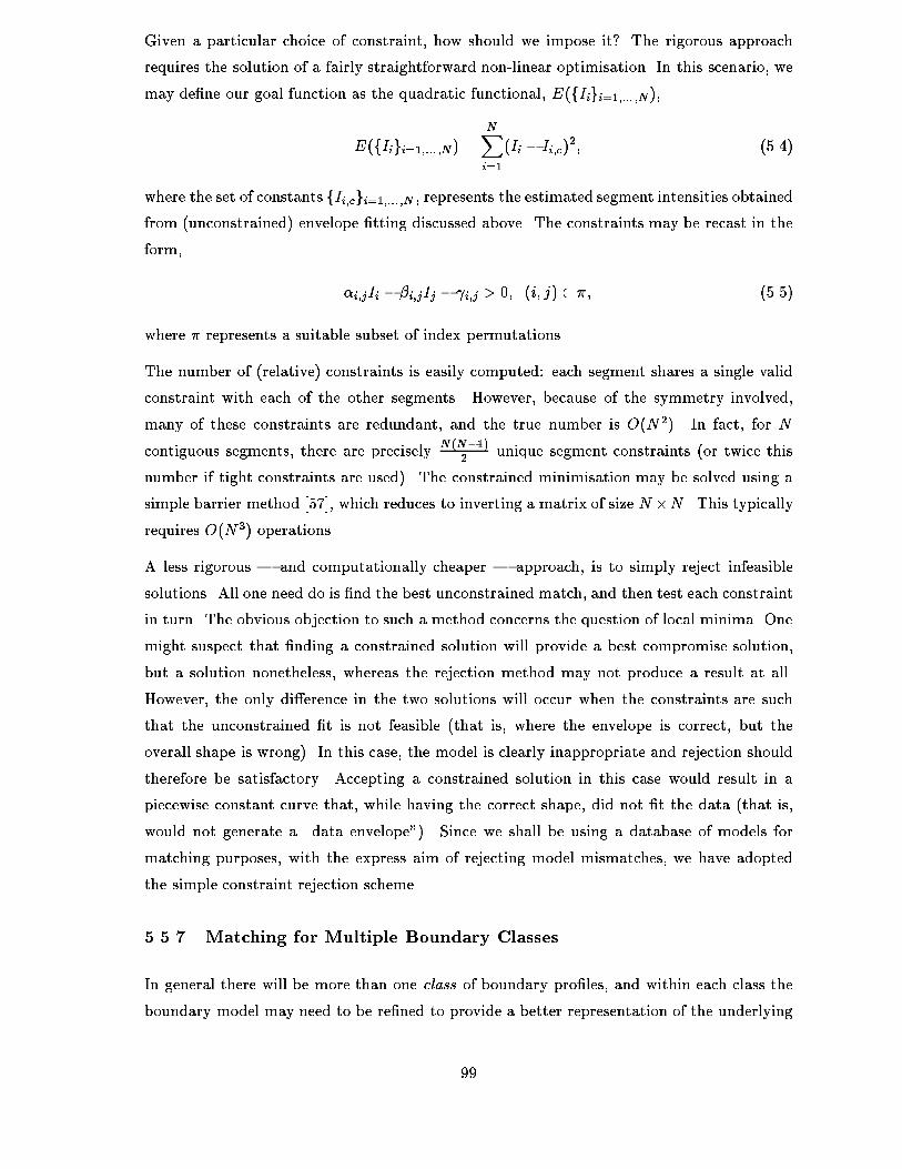
Given a particular choice of constraint� how should we impose it' The rigorous approach

requires the solution of a fairly straightforward nonlinear optimisation� In this scenario� we

may de�ne our goal function as the quadratic functional� E fIigi�� N��

E fIigi�� N� �NXi��

Ii � Ii�c��

where the set of constants fIi�cgi�� N � represents the estimated segment intensities obtainedfrom unconstrained� envelope �tting discussed above� The constraints may be recast in the

form�

�i�jIi � i�jIj � �i�j � �� i� j� � ��

where � represents a suitable subset of index permutations�

The number of relative� constraints is easily computed� each segment shares a single valid

constraint with each of the other segments� However� because of the symmetry involved�

many of these constraints are redundant� and the true number is O N�� In fact� for N

contiguous segments� there are precisely N�N�� unique segment constraints or twice this

number if tight constraints are used�� The constrained minimisation may be solved using a

simple barrier method �� which reduces to inverting a matrix of size N �N � This typicallyrequires O N�� operations�

A less rigorous � and computationally cheaper � approach� is to simply reject infeasible

solutions� All one need do is �nd the best unconstrained match� and then test each constraint

in turn� The obvious objection to such a method concerns the question of local minima� One

might suspect that �nding a constrained solution will provide a best compromise solution�

but a solution nonetheless� whereas the rejection method may not produce a result at all�

However� the only di�erence in the two solutions will occur when the constraints are such

that the unconstrained �t is not feasible that is� where the envelope is correct� but the

overall shape is wrong�� In this case� the model is clearly inappropriate and rejection should

therefore be satisfactory� Accepting a constrained solution in this case would result in a

piecewise constant curve that� while having the correct shape� did not �t the data that is�

would not generate a �data envelope�� Since we shall be using a database of models for

matching purposes� with the express aim of rejecting model mismatches� we have adopted

the simple constraint rejection scheme�

�� Matching for Multiple Boundary Classes

In general there will be more than one class of boundary pro�les� and within each class the

boundary model may need to be re�ned to provide a better representation of the underlying

��

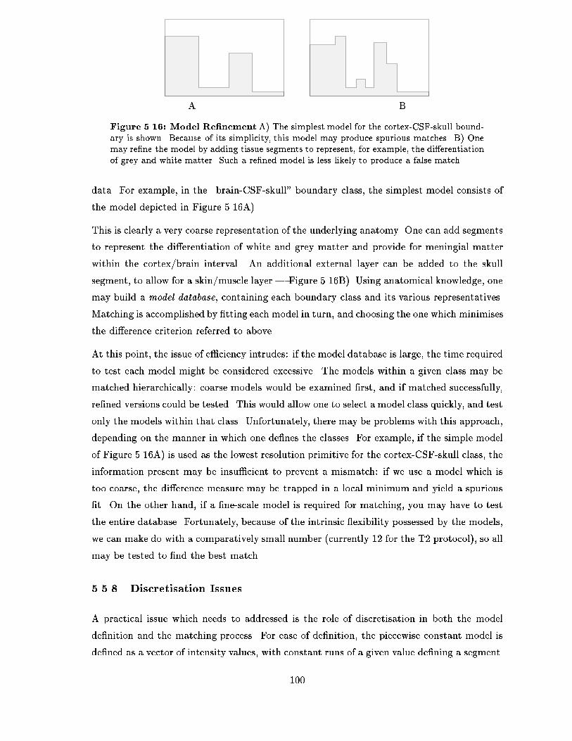
A B

Figure �� Model Re�nementA� The simplest model for the cortex�CSF�skull bound�ary is shown� Because of its simplicity� this model may produce spurious matches� B� Onemay re�ne the model by adding tissue segments to represent� for example� the di�erentiationof grey and white matter� Such a re�ned model is less likely to produce a false match�

data� For example� in the �brainCSFskull boundary class� the simplest model consists of

the model depicted in Figure ��A��

This is clearly a very coarse representation of the underlying anatomy� One can add segments

to represent the di�erentiation of white and grey matter and provide for meningial matter

within the cortex�brain interval� An additional external layer can be added to the skull

segment� to allow for a skin�muscle layer � Figure ��B�� Using anatomical knowledge� one

may build a model database� containing each boundary class and its various representatives�

Matching is accomplished by �tting each model in turn� and choosing the one which minimises

the di�erence criterion referred to above�

At this point� the issue of e�ciency intrudes� if the model database is large� the time required

to test each model might be considered excessive� The models within a given class may be

matched hierarchically� coarse models would be examined �rst� and if matched successfully�

re�ned versions could be tested� This would allow one to select a model class quickly� and test

only the models within that class� Unfortunately� there may be problems with this approach�

depending on the manner in which one de�nes the classes� For example� if the simple model

of Figure ��A� is used as the lowest resolution primitive for the cortexCSFskull class� the

information present may be insu�cient to prevent a mismatch� if we use a model which is

too coarse� the di�erence measure may be trapped in a local minimum and yield a spurious

�t� On the other hand� if a �nescale model is required for matching� you may have to test

the entire database� Fortunately� because of the intrinsic �exibility possessed by the models�

we can make do with a comparatively small number currently �� for the T� protocol�� so all

may be tested to �nd the best match�

�� Discretisation Issues

A practical issue which needs to addressed is the role of discretisation in both the model

de�nition and the matching process� For ease of de�nition� the piecewise constant model is

de�ned as a vector of intensity values� with constant runs of a given value de�ning a segment�

��

The model is matched to another discrete entity� the �D array of extracted pixel intensities�

If the data is sampled at a spatial frequency which is very di�erent from that represented by

the discrete model� the resulting model elements may be too large or small to represent the

equivalent features in the signal�

The sample size� �R� of the local symmetric step edge will determine the accuracy with which

edges may be localised under our edge de�nition�� In the extreme case in which R � �� the

step will be represented by only two samples� one having the value of the bottom of the step�

and one having the value at the top� Attempting to evaluate the optimum local �t using such

a step will almost certainly lead to disaster� since it has no averaging properties and is highly

susceptible to noise� On the other hand� if R is too large� the local step might not be able

to move at all� since it is forbidden from overrunning neighbouring edges� Alternatively� the

structure may be smaller than R� in which case we may fail to detect it�

We have a simple way of coping with these issues� we upsample both the signal and model�

Although this does not eliminate the problems� it reduces their severity and enables us to

utilise other heuristics to choose a reasonable value for R� The rationale behind this is as

follows�

Discretisation problems are primarily caused by undersampling of the continuous signaland�or model�

By linearly interpolating the input by a factor of L that is inserting L regularly sampled points on the line joining each pair of adjacent data points� we may increase the

sampling rate as much as we wish� whilst preserving the original signal structure�

By scaling the model in a similar fashion� but ensuring that we do not smear the edges�we may preserve the original spatial�intensity relationship between the signal and the

model�

If we �t our upsampled data with the upsampled model� the local re�nement scale� R�can be chosen to provide good matching�averaging characteristics� without having to

worry too much about edge mobility etc�

The choice of R was determined experimentally� The model and data were upsampled at

a speci�ed rate L� and the smallest reasonable value of R for a given L was recorded� In

general� the choice of L and R will depend on the sample length of the signal and model�

However� a reasonable heuristic seems to be L � �R� since this will ensure that the step sizeis roughly the same as the interval between two samples in the original signal� For the model

and signal lengths we used� L � � and R � � were found to be adequate�

��

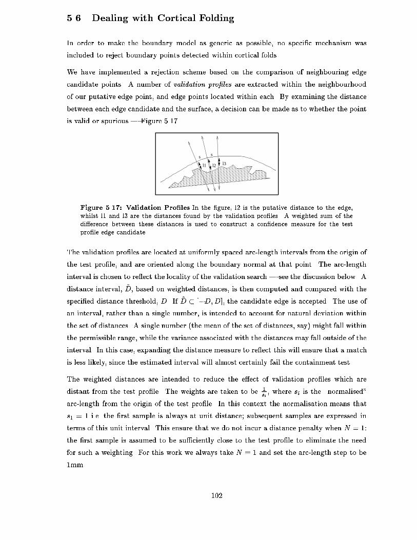
�� Dealing with Cortical Folding

In order to make the boundary model as generic as possible� no speci�c mechanism was

included to reject boundary points detected within cortical folds�

We have implemented a rejection scheme based on the comparison of neighbouring edge

candidate points� A number of validation pro�les are extracted within the neighbourhood

of our putative edge point� and edge points located within each� By examining the distance

between each edge candidate and the surface� a decision can be made as to whether the point

is valid or spurious � Figure ��

s s

l1 l2 l3��

��

��

��

��

��

��

��

��

��

��

��

��

��

Figure �� Validation Pro�les In the �gure� l� is the putative distance to the edge�whilst l and l� are the distances found by the validation pro�les� A weighted sum of thedi�erence between these distances is used to construct a con�dence measure for the testpro�le edge candidate�

The validation pro�les are located at uniformly spaced arclength intervals from the origin of

the test pro�le� and are oriented along the boundary normal at that point� The arclength

interval is chosen to re�ect the locality of the validation search � see the discussion below� A

distance interval� (D� based on weighted distances� is then computed and compared with the

speci�ed distance threshold� D� If (D � ��D�D�� the candidate edge is accepted� The use ofan interval� rather than a single number� is intended to account for natural deviation within

the set of distances� A single number the mean of the set of distances� say� might fall within

the permissible range� while the variance associated with the distances may fall outside of the

interval� In this case� expanding the distance measure to re�ect this will ensure that a match

is less likely� since the estimated interval will almost certainly fail the containment test�

The weighted distances are intended to reduce the e�ect of validation pro�les which are

distant from the test pro�le� The weights are taken to be �si� where si is the �normalised

arclength from the origin of the test pro�le� In this context the normalisation means that

s� � � i�e� the �rst sample is always at unit distance! subsequent samples are expressed in

terms of this unit interval� This ensure that we do not incur a distance penalty when N � ��

the �rst sample is assumed to be su�ciently close to the test pro�le to eliminate the need

for such a weighting� For this work we always take N � � and set the arclength step to be

�mm�

��

The algorithm is as follows�

Algorithm � � �Boundary Point Validation�

�� Extract a test pro�le at the point under consideration�� Extract N validation pro�les on either side of the test pro�le�� Compute the best edge point estimate for each pro�le�� Compute the signed distance� #i from the origin of each pro�le

to the corresponding edge location� The sign indicates whichside of the boundary curve the edge is located on the signof the test edge is always taken to be positive��

�� Construct the distance interval� (D � �Dw � �p�� Dw �

p��

where � is a constant which we take as �� Dw is the weightedaverage distance� and �� is the variance of theweighted distances� The weighted distances are de�ned as��i �

�sik#� �#ik�

The mean� Dw � and variance� �� are computed as per

normal� #� is the positive� distance from origin oftest pro�le to the prospective edge point�

�� If the interval (D � ��D�D�� then the edge point is accepted�

The algorithm is also applicable to �D edge searches� In this case the validation pro�les

would be centred on a set of surface points� arranged about the origin of the test pro�le a

symmetric distribution� for example� and the associated pro�les would be directed normal to

surface at the corresponding point�

The rejection mechanism will also �lter out obvious mismatches resulting from the boundary

detection stage� Such mismatches may occur if the pro�le contains structures not accounted

for in the model database�

�� Boundary Detection Results

The boundary detection results were obtained by running the segmentation scheme through

the initialisation phase� and noting the locations of detected boundary points� The full

segmentation scheme is introduced in Chapter �� It should be noted that the surface which

results from initialisation will not provide optimal conditions for edge point detection� since

it may be quite distant from the boundary of interest over certain regions�

�� Model Setup and Parameters

We built a model database consisting of �� piecewise constant models� This number could

have been reduced if a more e�cient model representation had been devised� The models

used are shown in Appendix F� They were chosen to re�ect the boundary pro�les within the

��

brain MR images we wished to segment� The two coarsest models were included to address

the issue of partial boundary occlusion� discussed in Section ��

The size of the pro�le sampling window was static� and set at ��mm� since this enabled us

to cover the boundary in most cases when the mesh surface was su�ciently close� If the

window is signi�cantly larger� then we may detect the other side of the brain� which will also

provide a valid boundary response� The development of strategies to cope with this problem

is considered to be a subject for future work�

The rejection mechanism was enabled� with N � � one validation search on either side of

the putative edge�� and D � ��mm� These values were chosen because they gave

reasonable results over the data sets we examined�

�� Results

The results presented in this section illustrate the range of boundary variation which the

models encompass� After the conclusion of the initial template alignment phase� the boundary

points along the mesh slice intersection curves were recorded� In Figures �� and �� a

number of slices from two quite di�erent brains are shown� Note that the extracted boundary

points are essentially correct� although only a few points are identi�ed in the topmost slice�

and the midsaggital line is missing� A subset of the edge models which are matched at various

boundary points are shown in Figure �� Note the range of variation which a given model

can represent� Although many boundaries present complex pro�les� the model is usually able

to make a sensible match�

�� Discussion

For the majority of slices� the boundary models provide good edge estimates� However� in the

uppermost slices� where foreshortening and PVE are maximal� the extracted boundary points

are less numerous� Examination of some of the pro�les � Figure �� shows that these

curves are punctuated by large� sharp peaks� corresponding to CSF which has penetrated the

sulci� In addition� there are sizeable dips in signal intensity which correspond to sulci which

are �lled with other matter� To �nd the boundary in this clutter is very di�cult� Only a

very coarse match can usually be obtained� and in many cases this match will be rejected

because the validation pro�les �nd very di�erent edge candidates�

The inclusion of the two coarse models referred to above allows us to detect boundaries

even when they are only partially covered by the sampling window� There are fairly strict

constraints on the permissible variation of these coarse models� This is necessary to prevent

them matching other� undesirable structures�

��

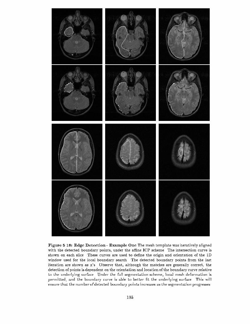
Figure �� Edge Detection Example One The mesh template was iteratively alignedwith the detected boundary points� under the a�ne ICP scheme� The intersection curve isshown on each slice� These curves are used to de�ne the origin and orientation of the Dwindow used for the local boundary search� The detected boundary points from the lastiteration are shown as xs� Observe that� although the matches are generally correct� thedetection of points is dependent on the orientation and location of the boundary curve relativeto the underlying surface� Under the full segmentation scheme� local mesh deformation ispermitted� and the boundary curve is able to better �t the underlying surface� This willensure that the number of detected boundary points increases as the segmentation progresses�

��

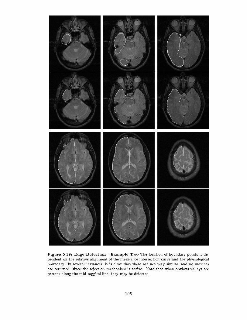
Figure �� Edge Detection Example Two The location of boundary points is de�pendent on the relative alignment of the mesh�slice intersection curve and the physiologicalboundary� In several instances� it is clear that these are not very similar� and no matchesare returned� since the rejection mechanism is active� Note that when obvious valleys arepresent along the mid�saggital line� they may be detected�

��

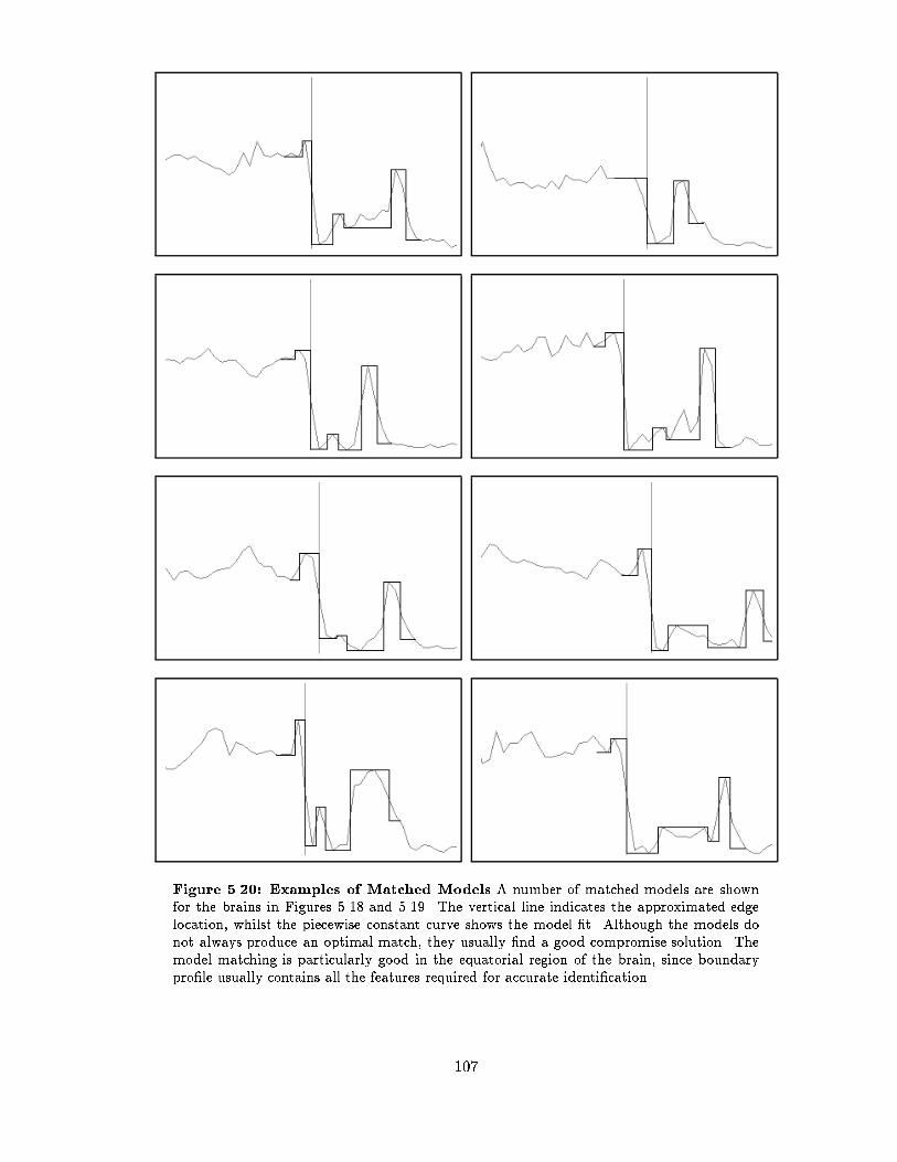
Figure �� Examples of Matched Models A number of matched models are shownfor the brains in Figures �� and �� The vertical line indicates the approximated edgelocation� whilst the piecewise constant curve shows the model �t� Although the models donot always produce an optimal match� they usually �nd a good compromise solution� Themodel matching is particularly good in the equatorial region of the brain� since boundarypro�le usually contains all the features required for accurate identi�cation�

��

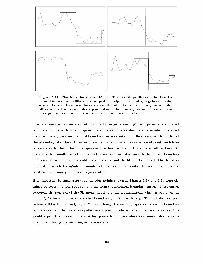
Figure �� The Need for Coarse Models The intensity pro�les extracted form thetopmost image slices are �lled with sharp peaks and dips� and warped by large foreshorteninge�ects� Boundary location in this case is very di�cult� The inclusion of very coarse modelsallows us to extract a reasonable approximation to the boundary� although in certain casesthe edge may be shifted from the ideal location �estimated visually��

The rejection mechanism is something of a twoedged sword� While it permits us to detect

boundary points with a fair degree of con�dence� it also eliminates a number of correct

matches� merely because the local boundary curve orientation di�ers too much from that of

the physiological surface� However� it seems that a conservative selection of point candidates

is preferable to the inclusion of spurious matches� Although the surface will be forced to

update with a smaller set of points� as the surface gravitates towards the correct boundary

additional correct matches should become visible and the �t can be re�ned� On the other

hand� if we selected a signi�cant number of false boundary points� the model update would

be skewed and may yield a poor segmentation�

It is important to emphasize that the edge points shown in Figures �� and �� were ob

tained by searching along rays emanating from the indicated boundary curves� These curves

represent the position of the �D mesh model after initial alignment� which is based on the

a�ne ICP scheme and uses extracted boundary points at each step� The initialisation pro

cedure will be detailed in Chapter �� Even though the initial proportion of visible boundary

points was small� the model was pulled into a position where many more became visible� One

would expect the proportion of matched points to improve when local mesh deformation is

introduced during the main segmentation stage�

��

�� Conclusion

In order to reliably identify points on the surface of the brain� we have introduced a database

of �exible boundary models and an algorithm to match these models to �D intensity data�

Modelling schemes based on heuristics and learning were considered and rejected� since they

could not provide the level of robustness we required� Rather than algorithmically attempting

to learn boundary structure from a set of training examples� the models are based directly

on our knowledge of expected boundary anatomy� Furthermore� the matching process used

to identify the required boundary points� provides us with the necessary infrastructure to

predict partial volume intensities � as we shall explain in Chapter ��

��

Chapter �

Modelling the Partial Volume

E�ect

The voxel size and anisotropy within sparse MR data combine to produce signi�cant partial

volumes Chapter �� Our objective is to accurately extract boundaries in the presence of

large PVE�

If we knew the volume of each tissue within a voxel� we could compute the expected MR

signal� Unfortunately� such information is not directly accessible� all we have to work with

are the recorded MR intensities� It is� however� possible to use this data to approximate the

local tissue geometry� as we shall show� This tissue model may then be used to predict local

voxel intensities� which may� in turn� be used to improve our boundary estimate�

The chapter starts by presenting a brief summary of related work� The MR imaging model we

shall use for our prediction scheme is then introduced� Section �� The prediction framework

is presented in Section �� and the manner in which the predicted intensities are employed

is discussed in Section �� Experimental results are presented in Section �� and discussed

in Section �� The chapter is concluded in Section ��

�� Related Work

Most of the work in the area of PVE analysis concerns the development of more reliable voxel

scale segmentation schemes� Many of the proposed solutions involve some sort of probabilistic

modelling �� with the aim of voxel classi�cation �� The data is usually highresolution�

rather than sparse and the MRI may be multimodal �� In a somewhat di�erent approach�

R)oll et al �� computes a partial volume correction based on an hypothesised model of PVE

variation� This is used to estimate the volume of objects with partially �lled boundary voxels�

An interesting approach adopted by Thacker et al� �� uses a number of specially chosen

imaging sequences to provide a set of equations which may be solved for each voxel to yield

��

estimates of tissue volumes� There is however� a limit to the number of tissues which may

be contained within any voxel� and the patient would have to be scanned several times�

introducing the possibility of image registration errors� This method is not applicable for

multimodal scans which do not satisfy their very stringent protocol constraints� nor can it

be retroactively applied to the kind of data we wish to analyse�

�� The MR Imaging model

We will assume the following idealised model for the signal from a voxel� which follows directly

from the physics of MR imaging ��

Linearity The observed voxel intensity� Iv� is a linearly weighted sum of the NT pure tissue

intensities� fIigi�� NT� arising from the NT tissue types present within the voxel�

Iv �

NTXi��

�iIi ��

Tissue Weights The tissue weights� �i� are given by

�i �Vi

V�

NTXi��

�i � ��

where V is the voxel volume and Vi is the volume of the tissue i present in the voxel� In other

words� the voxel intensity contribution of a given tissue class is proportional to the amount

of that tissue within the voxel� This model is an idealisation� albeit a common one ��

since the RF pulse used to select the image slice will always introduce intensity information

from neighbouring slices see Chapter �� This has the e�ect of blurring the voxel intensities

somewhat! however� the model provides a satisfactory approximation for our purposes�

In general� it is not possible to recover the volumes of tissue within a voxel� and one is forced

to estimate the �i directly� In certain cases� however� anatomical knowledge may be mobilised

to simplify the problem�

�� The Prediction Scheme

The preliminary matching stage� discussed in Section �� provides a local piecewise constant

boundary description at each point on the meshslice intersection curve� This description

is really an inplane� foreshortened approximation of the intensity pro�le sampled along the

surface normal at that point� Given a particular location on the boundary� and an estimate

of the surface normal at that point� we may use the piecewise constant model to estimate

��

the tissue arrangement within each voxel� and hence the volume contribution of each tissue

type� �i� to the associated voxel� The estimated tissue class intensities� Ii� which are already

implicit in the model and do not need to be computed� may then be combined with the tissue

weights under Equation �� to yield the expected voxel intensity�

Voxel

Local SurfaceApproximation

Direction of (approximated) Boundary Profile

Boundary Profile

Tissue 1

Tissue 2

Tissue 4

Tissue 3

Figure �� Voxel Partial VolumeFor each voxel� an approximation to the local boundarypro�le is generated which provides an estimate of the tissue organisation in the voxel� Wecan compute the volumes of each of these �approximately homogeneous� tissue regions anduse these to predict the voxel value�

The use of a �D piecewise constant model to approximate the local tissue distribution is

justi�ed if we make two assumptions�

�� the surface boundary is locally planar� and

�� each tissue��uid segment is considered to have a constant length over this local planar

region�

Such a planar laminar tissue arrangement is shown in Figure �� Any point on the mesh

surface has an associated �D laminar element of this type� which approximates the tissue

geometry in the voxel neighbourhood� Thus� if we know which laminar element a�ects a

given voxel� we will be able to intersect the associated sequence of planes with the voxel

and hence compute the nominal tissue decomposition for that voxel� Once such a polyhedral

decomposition is available� we simply compute the tissue volumes and for each class and

apply Equation ��

The volume of each polyhedron may be precisely computed from Gauss� Theorem� by sub

dividing each face into triangles and evaluating

V � k��

NtXi��

vi�� vi�� vi��k� ��

where Nt is the number of triangles and fvi�kg is the kth vertex of the ith triangle� Note thatthe order of evaluation must be consistent for each triangle which is viewed as an oriented

surface element��

For each voxel� the boundary model selected to generate the laminar element is the one

associated with the closest point� P � on the surface� since this point is likely to have the most

��

��

��

��

��

��

��

��

��

y

Surface Tissue Distribution

Surface Normal

r

BZ

Voxel Sampling Line

x

Surface Intersection Curve

Voxel Sample Liner

Z

A

Sample (image) Plane

C

P

BoundaryTransition

Voxel

Surface Intersection Curve

Piecewise TissueModel

Figure �� Prediction of Local Intensities A� The mesh is intersected by the imagingplane to yield a contour within the plane� For any voxel near this contour� we may predictthe intensity using the local piecewise constant boundary model� B� A D array of voxels isextracted along a ray normal to the boundary� This set of voxels will intersect the boundarytissue distribution� which we shall assume is locally laminar� C� The D local piecewise con�stant boundary model� representing the coarse initial �t� is then expanded to a �D �laminarelement which decomposes the voxel into a series of disjoint convex polyhedra� The volumesof these polyhedra are used to predict the voxel intensity� This �D cross�section shows howthe laminar element is shifted along the surface normal so that it is properly positioned forthe decomposition calculation�

anatomically relevant model� The surface normal at P provides the orientation of the model

i�e� the axis along which the transition planes are oriented� Having oriented the model in

space� all that remains to be done is to �attach it to the surface at P � Since each plane

corresponds to a particular tissue boundary� and we know which boundary the surface is

meant to represent� we slide the model along the normal until the correct plane coincides

with P � This is illustrated in Figure ��C�� which shows a �D crosssection of the voxel and

the decomposition resulting from the model alignment�

For a given voxel� the intensity prediction algorithm is as follows�

Algorithm � � �Voxel Prediction�

�� Obtain an estimate of local oriented boundary model�� Treat each tissue transition in this pro�le as the origin

of a plane which is oriented in the direction of the modelaxis � Figure ��

�� Compute the intersections of each transition plane with thevoxel and de�ne the bounding polyhedron for each tissue class�

�� Evaluate the volume� Vk� of each tissue polyhedron and

compute �k asVkV�

�� Predicted intensity is I �PNT

k�� kIk�

In itself the predicted intensity is of little use to us � we have already discussed the inap

��

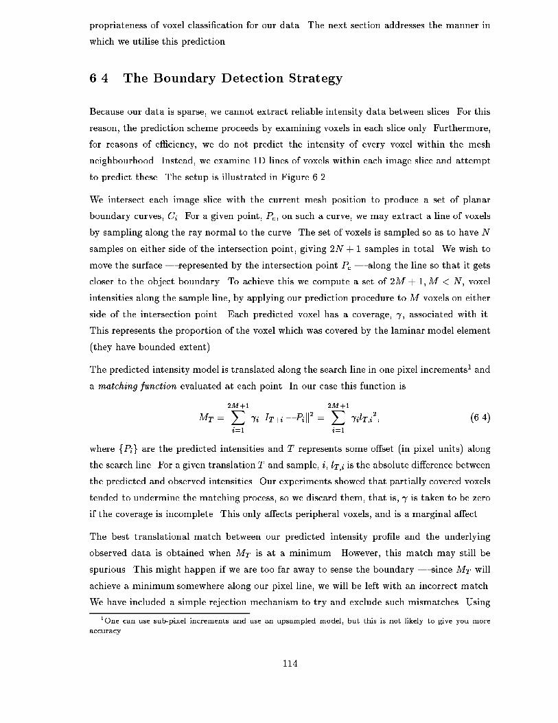
propriateness of voxel classi�cation for our data� The next section addresses the manner in

which we utilise this prediction�

�� The Boundary Detection Strategy

Because our data is sparse� we cannot extract reliable intensity data between slices� For this

reason� the prediction scheme proceeds by examining voxels in each slice only� Furthermore�

for reasons of e�ciency� we do not predict the intensity of every voxel within the mesh

neighbourhood� Instead� we examine �D lines of voxels within each image slice and attempt

to predict these� The setup is illustrated in Figure ��

We intersect each image slice with the current mesh position to produce a set of planar

boundary curves� Ci� For a given point� Pc� on such a curve� we may extract a line of voxels

by sampling along the ray normal to the curve� The set of voxels is sampled so as to have N

samples on either side of the intersection point� giving �N � samples in total� We wish to

move the surface � represented by the intersection point Pc � along the line so that it gets

closer to the object boundary� To achieve this we compute a set of �M ��M � N� voxel

intensities along the sample line� by applying our prediction procedure toM voxels on either

side of the intersection point� Each predicted voxel has a coverage� �� associated with it�

This represents the proportion of the voxel which was covered by the laminar model element

they have bounded extent��

The predicted intensity model is translated along the search line in one pixel increments� and

a matching function evaluated at each point� In our case this function is

MT ��M��Xi��

�ikIT�i � Pik� ��M��Xi��

�ilT�i��

where fPig are the predicted intensities and T represents some o�set in pixel units� alongthe search line� For a given translation T and sample� i� lT�i is the absolute di�erence between

the predicted and observed intensities� Our experiments showed that partially covered voxels

tended to undermine the matching process� so we discard them� that is� � is taken to be zero

if the coverage is incomplete� This only a�ects peripheral voxels� and is a marginal a�ect�

The best translational match between our predicted intensity pro�le and the underlying

observed data is obtained when MT is at a minimum� However� this match may still be

spurious� This might happen if we are too far away to sense the boundary � since MT will

achieve a minimum somewhere along our pixel line� we will be left with an incorrect match�

We have included a simple rejection mechanism to try and exclude such mismatches� Using

�One can use sub�pixel increments and use an upsampled model� but this is not likely to give you more

accuracy�

��

Figure �� Pro�le Prediction and Matching This image shows how the predictedpro�le �white dotted line� has been matched with the real intensity data in the image �thingrey line�� The vertical line indicates the position of the edge estimated through the matchingprocess�

flT�ig� an absolute �measure of goodness is computed for each tentative match� The measurelies between � and � and is computed as

p � ��

q��d

maxD� ��

where the variance �d and the maximum absolute di�erence� maxD� are computed over

flT�ig� Since there is usually a large discrepancy between a boundaries and spurious pro�les�a suitable threshold may be established by empirical means�

The end result of this process is a displacement vector in the plane� for Pc� indicating where

the mesh intersection point which corresponds to the boundary of interest� wishes to move�

Figure �� shows the predicted intensity pro�le for a point on a mesh object sphere� and

indicates the best match� under MT � with the real inplane intensity data� The vertical line

indicates the associated edge estimate� The match is in a plane raised from the equator by

about �� of the sphere�s radius�

�� Experiments on Synthetic Data

These experiments are intended to evaluate the robustness of the prediction scheme�

�� when we have perfect data�

�� when there is image noise�

�� when there is noise in the boundary model approximation�

To allow us access to ground truth� we have utilised analytically de�ned test objects�

��

��

��A

BA B

Figure �� Synthetic Volumetric Data A sphere composed of several tissue classes�represented by a unique intensity� A� shows a slice near the equator while B� shows a sectionfrom the poles� PVE was simulated by recursive voxel sub�division�

�� Test Data

The test objects consisted of a variety of spheres with shells of di�erent �tissue near the

surface� These tissue types are represented by di�erent absolute intensities� Partial volume

e�ects are simulated by recursive subdivision of voxels using the sphere formulae to determine

intensity values at subvoxel scales� The voxel dimensions were �� mm� with

a �mm gap� since this corresponds to the sampling protocol used to collect the data used in

this thesis� Typical crosssectional images are shown in Figure ��

Our spherical model has a range of tissue shells varying in thickness from ��mm� since

this corresponds to the level of detail within the boundary of interest� For the synthetic

data presented here� the boundary models are static and known a priori so no additional

processing is required�

�� Quantifying Edge Estimation Errors

The surface will intersect the predicted intensity pro�le at the centre of the computed voxel

span� As the predicted pro�le slides along the line of intensities� one may think of it as

pulling the �embedded surface along with it� We can compute the location of the edge

given by the �nal position of the centre of pro�le model� in �D� Likewise� for the series of

analytic shapes we have investigated� we can compute the true edge position along the line

of extracted pixels�

Thus� we have a means of computing the discrepancy between ground truth and our estimate

of edge location� The statistics given here are based on slicewise averaging of absolute

distances� For each slice� we can compute the absolute di�erence between the true and

approximated edges in mm� and then generate the mean of standard deviation of this set

of measurements� We can also compute the angle the sampling plane makes with the surface

normal on each slice this is constant for the shapes we have investigated! in general� this need

not be so�� We use the angle to index the statistics� Negative angles index measures from

��

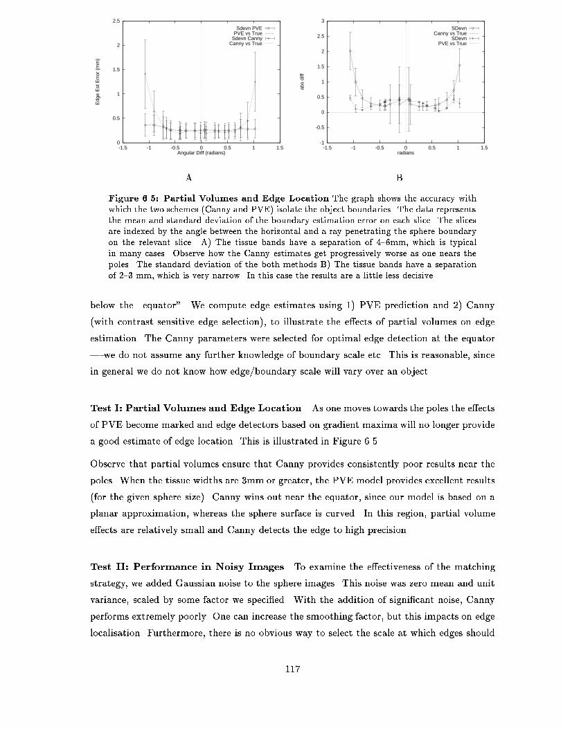
0

0.5

1

1.5

2

2.5

-1.5 -1 -0.5 0 0.5 1 1.5

Edg

e E

st E

rror

(m

m)

Angular Diff (radians)

Sdevn PVEPVE vs True

Sdevn CannyCanny vs True

-1

-0.5

0

0.5

1

1.5

2

2.5

3

-1.5 -1 -0.5 0 0.5 1 1.5

abs

diff

radians

SDevnCanny vs True

SDevnPVE vs True

A B

Figure �� Partial Volumes and Edge Location The graph shows the accuracy withwhich the two schemes �Canny and PVE� isolate the object boundaries� The data representsthe mean and standard deviation of the boundary estimation error on each slice� The slicesare indexed by the angle between the horizontal and a ray penetrating the sphere boundaryon the relevant slice� A� The tissue bands have a separation of ��mm� which is typicalin many cases� Observe how the Canny estimates get progressively worse as one nears thepoles� The standard deviation of the both methods B� The tissue bands have a separationof �� mm� which is very narrow� In this case the results are a little less decisive�

below the �equator� We compute edge estimates using �� PVE prediction and �� Canny

with contrast sensitive edge selection�� to illustrate the e�ects of partial volumes on edge

estimation� The Canny parameters were selected for optimal edge detection at the equator

� we do not assume any further knowledge of boundary scale etc� This is reasonable� since

in general we do not know how edge�boundary scale will vary over an object�

Test I� Partial Volumes and Edge Location As one moves towards the poles the e�ects

of PVE become marked and edge detectors based on gradient maxima will no longer provide

a good estimate of edge location� This is illustrated in Figure ��

Observe that partial volumes ensure that Canny provides consistently poor results near the

poles� When the tissue widths are �mm or greater� the PVE model provides excellent results

for the given sphere size�� Canny wins out near the equator� since our model is based on a

planar approximation� whereas the sphere surface is curved� In this region� partial volume

e�ects are relatively small and Canny detects the edge to high precision�

Test II� Performance in Noisy Images To examine the e�ectiveness of the matching

strategy� we added Gaussian noise to the sphere images� This noise was zero mean and unit

variance� scaled by some factor we speci�ed� With the addition of signi�cant noise� Canny

performs extremely poorly� One can increase the smoothing factor� but this impacts on edge

localisation� Furthermore� there is no obvious way to select the scale at which edges should

��

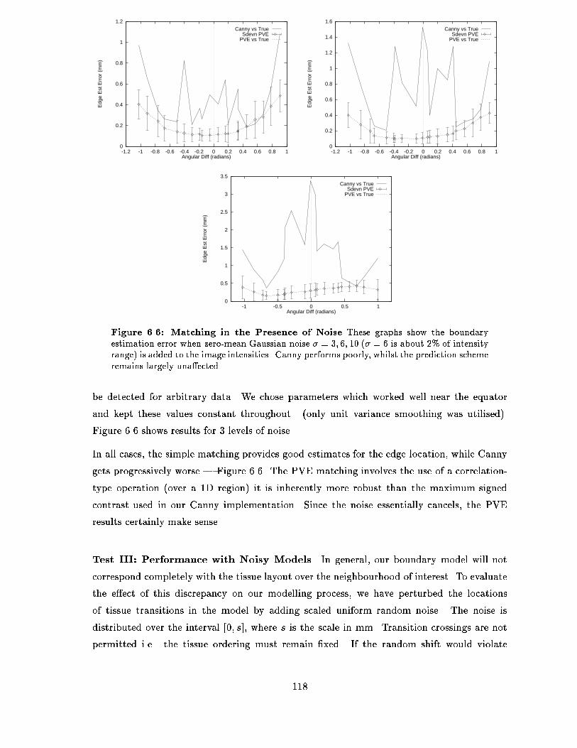
0

0.2

0.4

0.6

0.8

1

1.2

-1.2 -1 -0.8 -0.6 -0.4 -0.2 0 0.2 0.4 0.6 0.8 1

Edg

e E

st E

rror

(m

m)


Canny vs TrueSdevn PVE

PVE vs True

0

0.2

0.4

0.6

0.8

1

1.2

1.4

1.6

-1.2 -1 -0.8 -0.6 -0.4 -0.2 0 0.2 0.4 0.6 0.8 1

Edg

e E

st E

rror

(m

m)



PVE vs True

0

0.5

1

1.5

2

2.5

3

3.5

-1 -0.5 0 0.5 1

Edg

e E

st E

rror

(m

m)



PVE vs True

Figure �� Matching in the Presence of Noise These graphs show the boundaryestimation error when zero�mean Gaussian noise � � �� is about �� of intensityrange� is added to the image intensities� Canny performs poorly� whilst the prediction schemeremains largely una�ected�

be detected for arbitrary data� We chose parameters which worked well near the equator

and kept these values constant throughout� only unit variance smoothing was utilised��

Figure �� shows results for � levels of noise�

In all cases� the simple matching provides good estimates for the edge location� while Canny

gets progressively worse � Figure �� The PVE matching involves the use of a correlation

type operation over a �D region� it is inherently more robust than the maximum signed

contrast used in our Canny implementation� Since the noise essentially cancels� the PVE

results certainly make sense�

Test III� Performance with Noisy Models In general� our boundary model will not

correspond completely with the tissue layout over the neighbourhood of interest� To evaluate

the e�ect of this discrepancy on our modelling process� we have perturbed the locations

of tissue transitions in the model by adding scaled uniform random noise� The noise is

distributed over the interval �� s�� where s is the scale in mm� Transition crossings are not

permitted i�e� the tissue ordering must remain �xed� If the random shift would violate

��

0

0.2

0.4

0.6

0.8

1

1.2

1.4

1.6

1.8

2

-1.5 -1 -0.5 0 0.5 1 1.5

Dis

t Est

Err

or (

mm

)


SdevnPVE vs True

0

0.2

0.4

0.6

0.8

1

1.2

1.4

1.6

1.8

2

-1.5 -1 -0.5 0 0.5 1 1.5

Dis

t Est

Err

or (

mm

)


SdevnPVE vs True

0

0.2

0.4

0.6

0.8

1

1.2

1.4

1.6

1.8

2

-1.5 -1 -0.5 0 0.5 1 1.5

Dis

t Est

Err

or (

mm

)


SdevnPVE vs True

0

0.2

0.4

0.6

0.8

1

1.2

1.4

1.6

1.8

2

-1.5 -1 -0.5 0 0.5 1 1.5D

ist E

st E

rror

(m

m)


SdevnPVE vs True

Figure �� Estimates with Model Noise � �mm sphere Two examples are shownwhich illustrate the e�ect on boundary localisation of perturbing the model transitions�The data is for the case of partial volume boundary matching� and the noise is uniformlydistributed over the interval �� mm� Even for the case of the ��mm sphere� the averagelocalisation error remains low�

this constraint� we take the average of the two transition locations to either side as its new

location� Figure �� shows some results for the very narrow tissue sphere ��mm� for the

case of �mm scaling�

Figure �� shows the results for the case of the ��mm sphere� For this object the prediction

is quite robust� even with the �mm noise�

However� the ��mm tissue boundary may provide a considerably less robust estimate when

�mm noise is applied to the model� Again� this makes sense� since the smallest tissue band

is only �mm wide�

IV� Noisy �non�ideal� Pro�le Estimates with noisy data Finally� we looked at noisy

boundary models in noisy data� The results shown in Figure �� show what happens for the

��mm models in this case� The results are still good in this case�

��

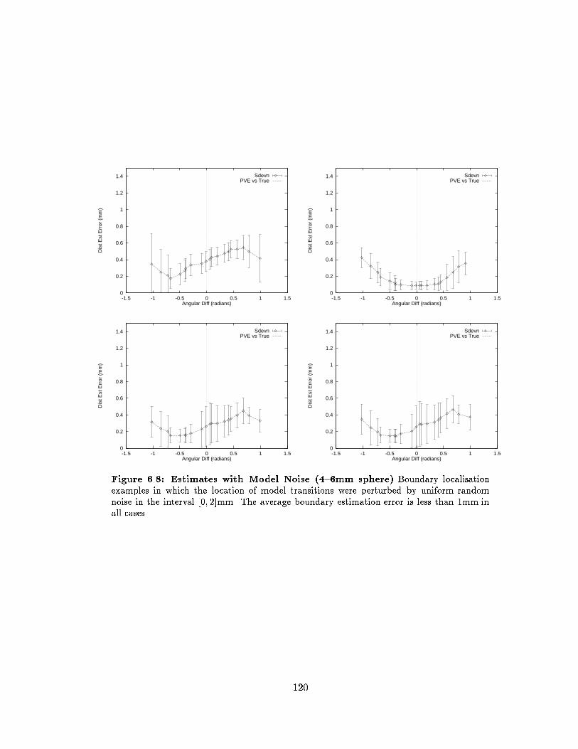
0

0.2

0.4

0.6

0.8

1

1.2

1.4

-1.5 -1 -0.5 0 0.5 1 1.5

Dis

t Est

Err

or (

mm

)


SdevnPVE vs True

0

0.2

0.4

0.6

0.8

1

1.2

1.4

-1.5 -1 -0.5 0 0.5 1 1.5

Dis

t Est

Err

or (

mm

)Angular Diff (radians)

SdevnPVE vs True

0

0.2

0.4

0.6

0.8

1

1.2

1.4

-1.5 -1 -0.5 0 0.5 1 1.5

Dis

t Est

Err

or (

mm

)


SdevnPVE vs True

0

0.2

0.4

0.6

0.8

1

1.2

1.4

-1.5 -1 -0.5 0 0.5 1 1.5

Dis

t Est

Err

or (

mm

)


SdevnPVE vs True

Figure �� Estimates with Model Noise ��mm sphere Boundary localisationexamples in which the location of model transitions were perturbed by uniform randomnoise in the interval �� mm� The average boundary estimation error is less than mm inall cases�

��

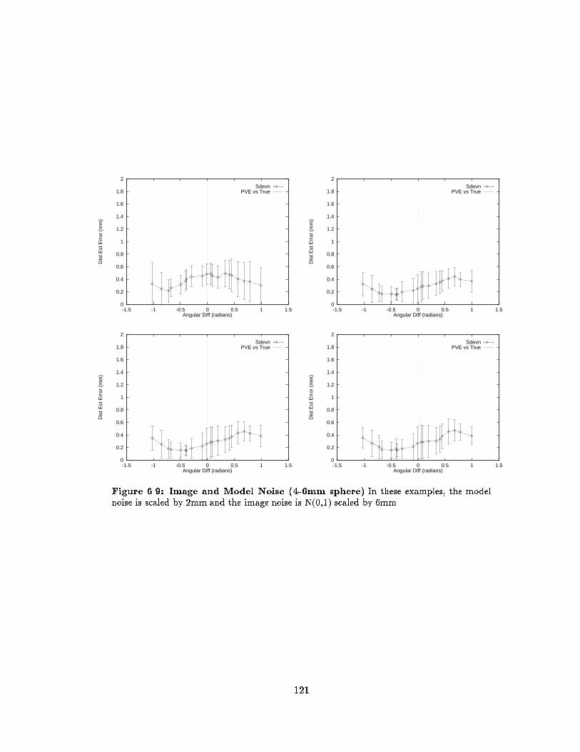
0

0.2

0.4

0.6

0.8

1

1.2

1.4

1.6

1.8

2

-1.5 -1 -0.5 0 0.5 1 1.5

Dis

t Est

Err

or (

mm

)


SdevnPVE vs True

0

0.2

0.4

0.6

0.8

1

1.2

1.4

1.6

1.8

2

-1.5 -1 -0.5 0 0.5 1 1.5D

ist E

st E

rror

(m

m)


SdevnPVE vs True

0

0.2

0.4

0.6

0.8

1

1.2

1.4

1.6

1.8

2

-1.5 -1 -0.5 0 0.5 1 1.5

Dis

t Est

Err

or (

mm

)


SdevnPVE vs True

0

0.2

0.4

0.6

0.8

1

1.2

1.4

1.6

1.8

2

-1.5 -1 -0.5 0 0.5 1 1.5

Dis

t Est

Err

or (

mm

)


SdevnPVE vs True

Figure �� Image and Model Noise � �mm sphere In these examples� the modelnoise is scaled by �mm and the image noise is N�� scaled by �mm�

��

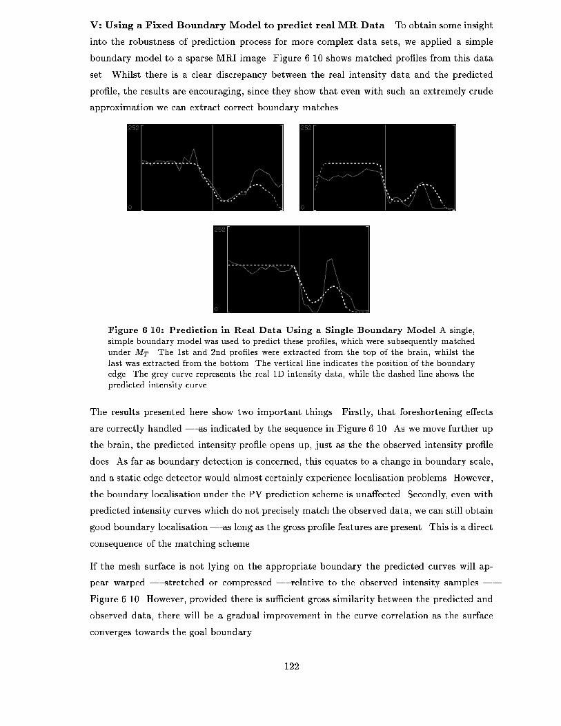
V� Using a Fixed Boundary Model to predict real MR Data To obtain some insight

into the robustness of prediction process for more complex data sets� we applied a simple

boundary model to a sparse MRI image� Figure �� shows matched pro�les from this data

set� Whilst there is a clear discrepancy between the real intensity data and the predicted

pro�le� the results are encouraging� since they show that even with such an extremely crude

approximation we can extract correct boundary matches�

Figure �� Prediction in Real Data Using a Single Boundary Model A single�simple boundary model was used to predict these pro�les� which were subsequently matchedunder MT � The st and �nd pro�les were extracted from the top of the brain� whilst thelast was extracted from the bottom� The vertical line indicates the position of the boundaryedge� The grey curve represents the real D intensity data� while the dashed line shows thepredicted intensity curve�

The results presented here show two important things� Firstly� that foreshortening e�ects

are correctly handled � as indicated by the sequence in Figure �� As we move further up

the brain� the predicted intensity pro�le opens up� just as the the observed intensity pro�le

does� As far as boundary detection is concerned� this equates to a change in boundary scale�

and a static edge detector would almost certainly experience localisation problems� However�

the boundary localisation under the PV prediction scheme is una�ected� Secondly� even with

predicted intensity curves which do not precisely match the observed data� we can still obtain

good boundary localisation� as long as the gross pro�le features are present� This is a direct

consequence of the matching scheme�

If the mesh surface is not lying on the appropriate boundary the predicted curves will ap

pear warped � stretched or compressed � relative to the observed intensity samples �

Figure �� However� provided there is su�cient gross similarity between the predicted and

observed data� there will be a gradual improvement in the curve correlation as the surface

converges towards the goal boundary�

��

�� Prediction Using Matched Models

If the boundary matching scheme outlined in Section �� has been applied� we may utilise

these models to de�ne the local laminar element at that point� The inplane model can

be subjected to a cosine foreshortening which will map it onto the direction of the surface

normal� and used to directly predict the intensities of the voxels in the immediate vicinity of

the boundary point�

This kind of matching is similar to that proposed above� but uses only the boundary model

located at the intersection point� rather than those further away� This initial scaled model

estimate may be re�ned in an attempt to obtain a better match in the vicinity of the edge

estimate�

The re�nement proceeds by brute force� the normal orientation and individual piecewise con

stant lengths are varied di�erentially� and the resulting predicted intensity curves compared

with the observed signal in the boundary point neighbourhood� By varying the normal ori

entation� we can account for misalignment of the local surface patch� which would otherwise

create spurious degradation in the predicted intensity� Varying the segment widths allows

also one to compensate for errors in the location of the closest surface point� This process is

very expensive� requiring an exponential number of partial voxel calculations which are in

dividually complex and expensive�� More speci�cally� if there are NT segments� which means

that NT � � transitions are to be varied� and each may be shifted into one of l di�erent locations� the number of voxel evaluations will be N�l

NT�� The value N� represents the number

of di�erent normal orientations which are tested� This number rapidly becomes large� and

given that a set of voxels at each boundary point is required for matching purposes� the time

required to traverse the search space may be excessive�� In general� the number of planes

intersecting a voxel will be less than or equal to three� � if this aspect could be exploited�

computation time could be accordingly reduced�

To test the usefulness of this scheme� the initial matched models were used to predict a local

intensity span� �� voxels in length� In this instance� only angular re�nement was permitted�

there was no di�erential modi�cation of segment widths� Nonetheless� the predicted curves

over much of the model were quite good � Figure �� The exception was found in the polar

regions of the brain� where the surface was not close to the boundary of interest� and the

boundaries have complex signatures� Figure ��A�D�� These results show that the scheme

is workable� provided improved estimates can be obtained for models at the top of the brain�

�Hours� perhaps� for a complex set of boundary models� a large number of voxels� and a reasonably �ne

parameter increment��There are seldom more than tissues in a voxel� or so empirical evidence would suggest�

��

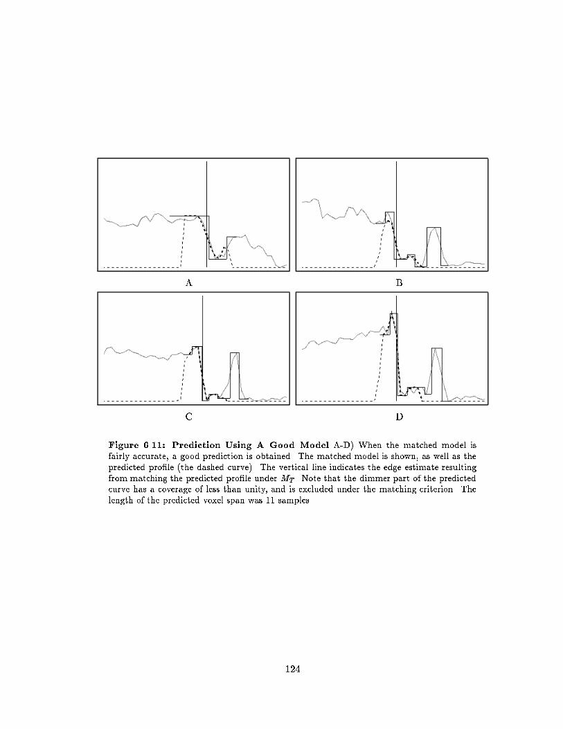
A B

C D

Figure �� Prediction Using A Good Model A�D� When the matched model isfairly accurate� a good prediction is obtained� The matched model is shown� as well as thepredicted pro�le �the dashed curve�� The vertical line indicates the edge estimate resultingfrom matching the predicted pro�le under MT � Note that the dimmer part of the predictedcurve has a coverage of less than unity� and is excluded under the matching criterion� Thelength of the predicted voxel span was samples�

��

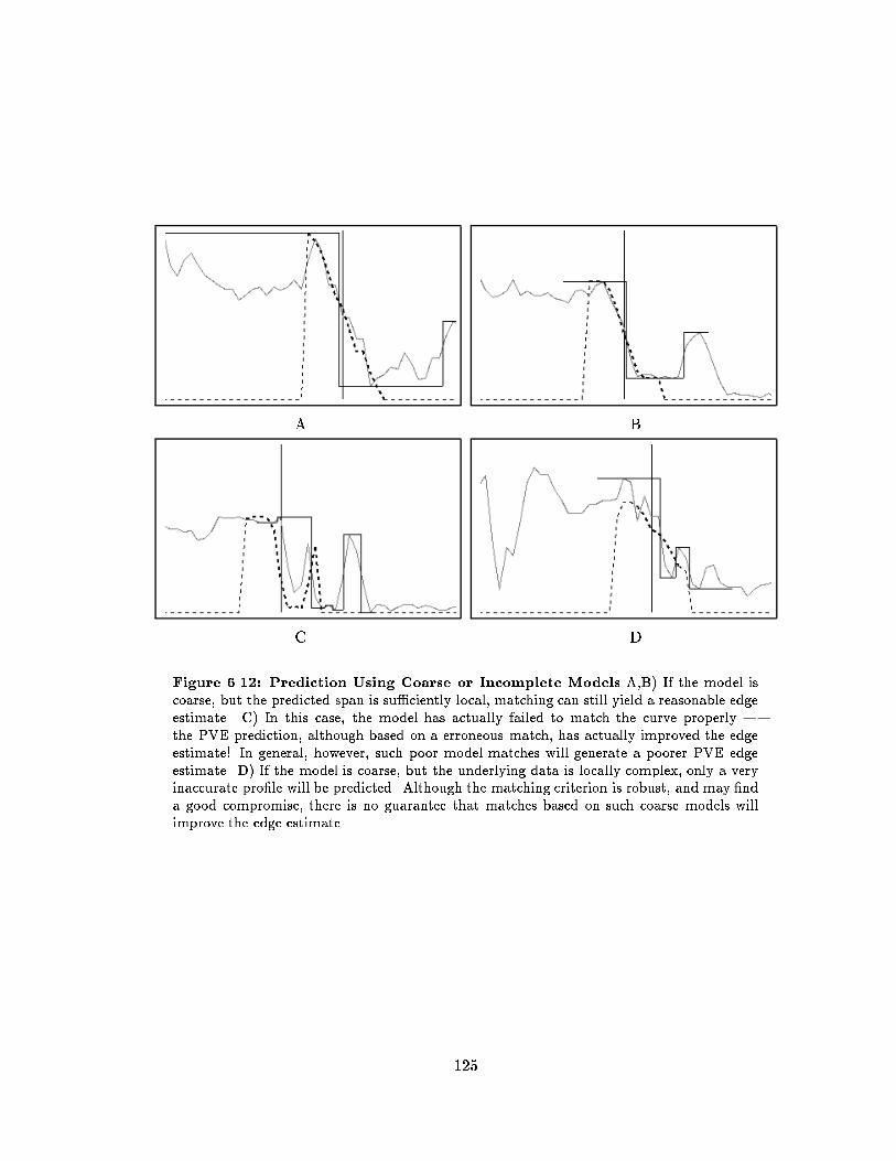
A B

C D

Figure �� Prediction Using Coarse or Incomplete Models A�B� If the model iscoarse� but the predicted span is su�ciently local� matching can still yield a reasonable edgeestimate� C� In this case� the model has actually failed to match the curve properly �the PVE prediction� although based on a erroneous match� has actually improved the edgeestimate! In general� however� such poor model matches will generate a poorer PVE edgeestimate� D� If the model is coarse� but the underlying data is locally complex� only a veryinaccurate pro�le will be predicted� Although the matching criterion is robust� and may �nda good compromise� there is no guarantee that matches based on such coarse models willimprove the edge estimate�

��

� Discussion

The sparse segmentation algorithm requires the calculation of the closest point on the surface

mesh to a given neighbourhood point� Clearly the sampling density of this surface will impact

on the accuracy with which we can approximate this point� We have experimented with spline

interpolants and the results seem to indicate that the planar approximation used is su�cient

for our purposes� Further indication of the robustness of the scheme may be deduced from

the experiments in which the boundary model transitions were perturbed� These experiments

showed that the prediction remains good even when the model is displaced from its correct

location�

The simple matching function we used proved adequate� Because it is a correlationtype

operator� it is also robust in the presence of noise and global luminance shifts� Furthermore�

the predicted inplane intensities do not have to be highly accurate for a good match� As

the predicted span becomes larger� there is a chance that the closest point will no longer be

located on the correct part of the surface� However� we have stressed that this segmentation

algorithm is only appropriate for local model updates�

The principal problem with this approach is the construction of a representative piecewise

constant model in the voxel neighbourhood� While the models generated by the initial bound

ary detection process provide just such a representation� this is often too coarse in the areas

in which PVE is most acute� However� if the initial model �t is assumed to provide a good

match� then it is still possible to use the model to predict a small voxel neighbourhood about

the edge� The most serious objection to this scheme arises from the poor model �ts obtained

at the top of the brain� These need to be improved if the PV prediction is to be useful in

this region�

� Conclusion

In this chapter� we have introduced a framework which enables us to predict partial volumes

in the vicinity of the surface model� These predicted values can be used to re�ne the local

boundary estimate� The prediction scheme is based on a local geometric construction� which

is generated directly from the matched boundary models resulting from the initial boundary

detection phase�

��

Chapter �

Surface�based Segmentation

The preceding chapters have established the infrastructure we require for our segmentation

scheme� For any given model position� the techniques introduced in Chapter � enable us

to generate a new set of �D data points� representing an improved estimate of the surface

we wish to extract� This chapter describes the process by which the current model position

will be updated� We desire an update strategy which will ensure that the resulting surface

smoothly interpolates the given data� whilst respecting our shape constraints Chapter ��

Once again the restrictions imposed by sparse acquisition must be considered� In particular�

signi�cant truncation and acquisition direction� subsampling artifacts must be accounted

for in the update scheme� Finally� the robustness of the entire scheme must be validated

against a set of examples for which we have some notion of ground truth�

The chapter begins with a brief overview of the active shape model ASM�� the basic mech

anism we shall use to enforce our shape constraints� Section �� introduces our extensions�

and explains why they are necessary� The issue of template initialisation is addressed in

Section �� In Section �� we give a detailed description of the segmentation strategy�

Segmentation results are presented in Section �� and analysed in Section �� Section ��

concludes this �nal chapter�

�� Utilising the Shape Constraint

The point distribution model� introduced in Chapter �� describes the permissible shape vari

ation a class of objects may exhibit� but does not include an algorithm to exploit this infor

mation during the segmentation process� The active shape model ASM� proposed by Cootes

and Taylor �� may be used for this purpose�

Under this scheme� a preferred displacement is computed for each mesh vertex� based on the

the available boundary data� The set of these vertex displacements � which represents the

model deformation� is then �projected into the PDM subspace to arrive at the permissible

��

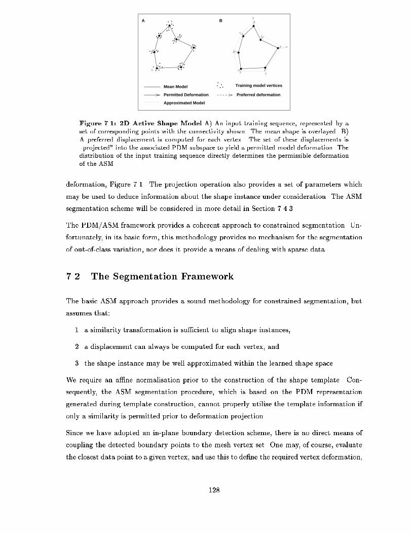
Permitted Deformation

BA

Mean Model

Approximated Model

Training model vertices

Preferred deformation

Figure �� D Active Shape Model A� An input training sequence� represented by aset of corresponding points with the connectivity shown� The mean shape is overlayed� B�A preferred displacement is computed for each vertex� The set of these displacements is�projected into the associated PDM subspace to yield a permitted model deformation� Thedistribution of the input training sequence directly determines the permissible deformationof the ASM�

deformation� Figure �� The projection operation also provides a set of parameters which

may be used to deduce information about the shape instance under consideration� The ASM

segmentation scheme will be considered in more detail in Section ��

The PDM�ASM framework provides a coherent approach to constrained segmentation� Un

fortunately� in its basic form� this methodology provides no mechanism for the segmentation

of outofclass variation� nor does it provide a means of dealing with sparse data�

�� The Segmentation Framework

The basic ASM approach provides a sound methodology for constrained segmentation� but

assumes that�

�� a similarity transformation is su�cient to align shape instances�

�� a displacement can always be computed for each vertex� and

�� the shape instance may be well approximated within the learned shape space�

We require an a�ne normalisation prior to the construction of the shape template� Con

sequently� the ASM segmentation procedure� which is based on the PDM representation

generated during template construction� cannot properly utilise the template information if

only a similarity is permitted prior to deformation projection�

Since we have adopted an inplane boundary detection scheme� there is no direct means of

coupling the detected boundary points to the mesh vertex set� One may� of course� evaluate

the closest data point to a given vertex� and use this to de�ne the required vertex deformation�

��

as in Delingette �� Unfortunately� due to the sparsity of the data� the resulting deformation

may produce a shape which is truncated or �attened�

The ASM is designed speci�cally to improve the robustness of segmentation by excluding

outofclass shape variation where the �inclass variability is encapsulated by the training

examples�� We require a means of segmenting outofclass structure� since we wish to inves

tigate pathology� However� we cannot simply discard the shape constraint� since this would

sacri�ce the robustness we have worked so hard to obtain� Furthermore� for clinical assess

ment� it would be useful to determine the extent to which a given shape instance varies from

the �normal range� The learned shape constraints enable us to estimate the best normal

approximation for the given shape instance�

In order to obtain a more descriptive segmentation� we require a scheme which will allow us

to smoothly and locally move away from our initial shape estimate� This new deformation

should respect the outcome of the �rst stage as far as possible� The segmentation approach

adopted by Montagnat �� see Section �� in Chapter �� uses a static simplex template to

perform constrained segmentation� The simplex template provides a reference shape which is

used to interpolate missing data� as well as locally constraining the permissible surface defor

mation� Unfortunately� the use of a static shape template may result in an overconstrained

segmentation� particularly for highly variable anatomy� However� since we have a patient

speci�c simplex model � the output of the ASM segmentation step � we can apply this

approach to generate a less constrained� more representative shape description�

In light of these observations� we have implemented the following segmentation strategy�

A�ne ASM The basic ASM is extended to include an A�ne normalisation�

Modi�ed Closest Point For each vertex� the closest data point is used to de�ne the re

quired displacement� The closest point de�nition is modi�ed to compensate for prob

lems arising from data sparsity and truncation� Furthermore� the distance between the

vertex and the closest data point determines the magnitude of the vertex displacement�

Two�Tier Segmentation The segmentation proceeds in two stages� In the �rst� the ASM is

employed to achieve a constrained segmentation� This provides the normal component

of the shape instance� In the second phase� the ASM constraint is dropped and the

deformation is allowed to proceed until the surface update method converges� For this

stage� a simplex template is used� which provides a means of preserving the basic shape

which emerges from initial segmentation�

The basic segmentation strategy is simple�

�� Map the model into the volumetric image�

��

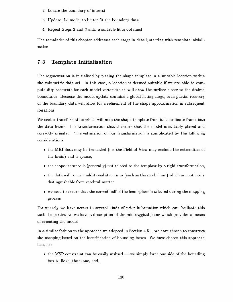
�� Locate the boundary of interest�

�� Update the model to better �t the boundary data�

�� Repeat Steps � and � until a suitable �t is obtained�

The remainder of this chapter addresses each stage in detail� starting with template initiali

sation�

�� Template Initialisation

The segmentation is initialised by placing the shape template in a suitable location within

the volumetric data set� In this case� a location is deemed suitable if we are able to com

pute displacements for each model vertex which will draw the surface closer to the desired

boundaries� Because the model update contains a global �tting stage� even partial recovery

of the boundary data will allow for a re�nement of the shape approximation in subsequent

iterations�

We seek a transformation which will map the shape template from its coordinate frame into

the data frame� The transformation should ensure that the model is suitably placed and

correctly oriented� The estimation of our transformation is complicated by the following

considerations�

the MRI data may be truncated i�e� the Field of View may exclude the extremities ofthe brain� and is sparse�

the shape instance is generally� not related to the template by a rigid transformation�

the data will contain additional structures such as the cerebellum� which are not easilydistinguishable from cerebral matter�

we need to ensure that the correct half of the hemisphere is selected during the mappingprocess�

Fortunately we have access to several kinds of prior information which can facilitate this

task� In particular� we have a description of the midsaggital plane which provides a means

of orienting the model�

In a similar fashion to the approach we adopted in Section �� we have chosen to construct

the mapping based on the identi�cation of bounding boxes� We have chosen this approach

because�

the MSP constraint can be easily utilised � we simply force one side of the bounding

box to lie on the plane� and�

��

the establishment of correspondences between the model and the shape instance isvery di�cult� if we knew the shape instance� our segmentation would be complete� In

contrast� the bounding box method provides a crude but robust way of computing our

desired transformation in which only a very rough idea of the shape instance location

is required � this can be obtained by simple thresholding�

The approach relies on the identi�cation of two object centred descriptions� one for the shape

template and one for the data instance�

�� Computing the Template Bounding Box

The construction of a mesh object bounding box and the inclusion of the MSP constraint

were discussed in Section �� The MSP was semiautomatically extracted for each brain

in the training set� using a propagating snake curve�

The template exists in a righthanded� canonical frame in which the plane normal is oriented

along the unit vector i� A principal components analysis� based on the convex hull of the entire

model point set projected onto this plane� provides two principal axes which are mapped onto

the remaining coordinate axes� j and k� The centroid of the resulting model bounding box

with axes along i� j�k� is projected onto the plane and mapped onto the origin� Using this

information together with our prior knowledge� we can identify the template type left�right

hemisphere! axial or coronal acquisition�� as well as its spatial extent represented by the

bounding box��

�� Computing the Shape Instance Bounding Box

The extraction of the shape instance bounding box requires the approximate� identi�cation

of the brain in each slice of the volumetric image� Because MR data is characterised by a

dark background for all protocols�� we can apply a simple thresholding technique to obtain

a binary image in which background corresponding to air and� possibly� the intracranial

cavity and ventricles� is black and all else is white� We do not� however� wish our binary

segmentation to contain the skull or any noncerebral matter� By selecting an appropriate

threshold and computing the largest connected component on each slice� we can essentially

eliminate the pixels associated with spurious structure�

The brain component within each slice may be placed within a �D bounding box de�ned

by its principal components� The longest medial line of the bounding box for axial scans�

provides a crude approximation to the midsaggital line� the accuracy of which depends on the

�Saggital scans are more di�cult to deal with� since they have no line of symmetry� We could ignore this

problem since our database did not contain any�

��

degree of headtilt and the location of the slice in the brain see below�� Points on these lines

from each slice may be used as input to a plane �tting procedure to estimate the MSP� Then�

applying the same procedure utilised in Section �� we may construct a planeconstrained

bounding box� suitable for use in the estimation of our transformation�

The following steps are applied for axial scans��

Thresholding The choice of the intensity threshold for each slice is problematic� If the value

is too low� unwanted structure emerges� Conversely� a high threshold may eliminate the

intensities we wish to detect� In general� there may be luminance changes from slice

to slice which make the selection of a global threshold untenable� One would expect�

however� that tissues will retain their relative intensity separation from slice to slice�

We have opted for a simple solution which works well on most slices� a prespeci�ed

cuto� of the dynamic range of intensities is chosen� More speci�cally� the threshold

value� It� given by

It � Imin r Imax � Imin��

where r � �� is �xed at �� for the data we wish to segment� This value was chosenempirically� by examining the results over a number of representative T�weighted�

data sets� The threshold will also adjust correctly under uniform intensity rescaling�

Largest Connected Component �LCC� We then compute the largest connected com�

ponent� Ci� for each slice� This will eliminate the skull and nonbrain matter if the

threshold has been set appropriately� There is usually a high level of image noise in

lower slices due to �ow artifacts� The combination of our thresholding procedure and

�connectivity appears to be su�cient to eliminate these points� The largest connected

component will usually encompass both hemispheres and in most cases� the cerebellum�

The inclusion of the cerebellum is not desirable� since this structure is not represented

within our model and may induce a large distortion of the bounding box estimate�

Most studies of gross brain asymmetry exclude the cerebellum� so if the results are

to be comparable� this structure must not be segmented� In order to remove obvious

cerebellar components� we apply the heuristic� area of cerebellar cross�section is less

than half of the largest axial cerebral cross�section� Of course� since the cerebellum is

on the underside of the brain� we do not apply this rule to the upper half of the brain�

This heuristic is rather crude� and assumes that the brain is roughly aligned with the

imaging axes� and that the scan is axial� In this case� the cerebellum is isolated from the

cerebrum on the bottommost slices� Fortunately� as we shall show� the initialisation

can be quite poor and still provide a satisfactory starting point for our segmentation

scheme�

Compute the Convex Hull of Ci The computed LCC may contain holes and concavities

��

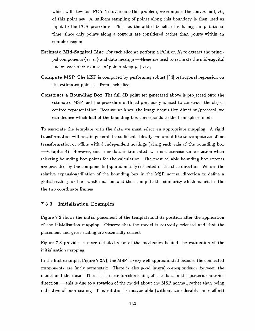
which will skew our PCA� To overcome this problem� we compute the convex hull� Hi�

of this point set� A uniform sampling of points along this boundary is then used as

input to the PCA procedure� This has the added bene�t of reducing computational

time� since only points along a contour are considered rather than points within an

complex region�

Estimate Mid�Saggital Line For each slice we perform a PCA on Hi to extract the princi

pal components fe�� e�g and data mean� �� these are used to estimate the midsaggital

line on each slice as a set of points along � � e��

Compute MSP The MSP is computed by performing robust �� orthogonal regression on

the estimated point set from each slice�

Construct a Bounding Box The full �D point set generated above is projected onto the

estimated MSP and the procedure outlined previously is used to construct the object

centred representation� Because we know the image acquisition direction�protocol� we

can deduce which half of the bounding box corresponds to the hemisphere model�

To associate the template with the data we must select an appropriate mapping� A rigid

transformation will not� in general� be su�cient� Ideally� we would like to compute an a�ne

transformation or a�ne with � independent scalings along each axis of the bounding box

� Chapter �� However� since our data is truncated� we must exercise some caution when

selecting bounding box points for the calculation� The most reliable bounding box extents

are provided by the components approximately� oriented in the slice direction� We use the

relative expansion�dilation of the bounding box in the MSP normal direction to de�ne a

global scaling for the transformation� and then compute the similarity which associates the

the two coordinate frames�

�� Initialisation Examples

Figure �� shows the initial placement of the template�and its position after the application

of the initialisation mapping� Observe that the model is correctly oriented and that the

placement and gross scaling are essentially correct�

Figure �� provides a more detailed view of the mechanics behind the estimation of the

initialisation mapping�

In the �rst example� Figure ��A�� the MSP is very well approximated because the connected

components are fairly symmetric� There is also good lateral correspondence between the

model and the data� There is is clear foreshortening of the data in the posterioranterior

direction � this is due to a rotation of the model about the MSP normal� rather than being

indicative of poor scaling� This rotation is unavoidable without considerably more e�ort�

��

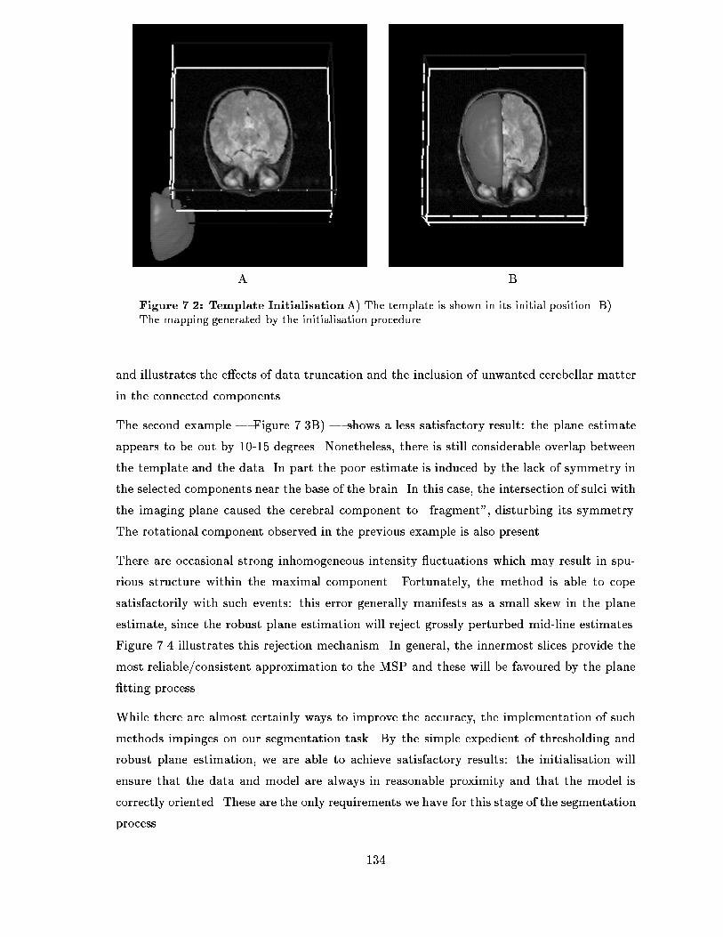
A B

Figure �� Template Initialisation A� The template is shown in its initial position� B�The mapping generated by the initialisation procedure�

and illustrates the e�ects of data truncation and the inclusion of unwanted cerebellar matter

in the connected components�

The second example � Figure ��B� � shows a less satisfactory result� the plane estimate

appears to be out by �� degrees� Nonetheless� there is still considerable overlap between

the template and the data� In part the poor estimate is induced by the lack of symmetry in

the selected components near the base of the brain� In this case� the intersection of sulci with

the imaging plane caused the cerebral component to �fragment� disturbing its symmetry�

The rotational component observed in the previous example is also present�

There are occasional strong inhomogeneous intensity �uctuations which may result in spu

rious structure within the maximal component� Fortunately� the method is able to cope

satisfactorily with such events� this error generally manifests as a small skew in the plane

estimate� since the robust plane estimation will reject grossly perturbed midline estimates�

Figure �� illustrates this rejection mechanism� In general� the innermost slices provide the

most reliable�consistent approximation to the MSP and these will be favoured by the plane

�tting process�

While there are almost certainly ways to improve the accuracy� the implementation of such

methods impinges on our segmentation task� By the simple expedient of thresholding and

robust plane estimation� we are able to achieve satisfactory results� the initialisation will

ensure that the data and model are always in reasonable proximity and that the model is

correctly oriented� These are the only requirements we have for this stage of the segmentation

process�

��

A

B

Figure �� Computing the Initialisation A� The �rst row of images shows the convexhull for the thresholded image data on a number of slices� and the resulting symmetryaxis estimate for each� Points from each symmetry axis are used to robustly estimate theMSP� which is used in conjunction with the thresholded data to compute the initialisationmapping� The second row of images shows the intersection curves of the initialised meshwith the corresponding slices� B� The MSP estimate may be quite poor in certain cases� butthe general orientation and position of the initialised model will be correct�

��

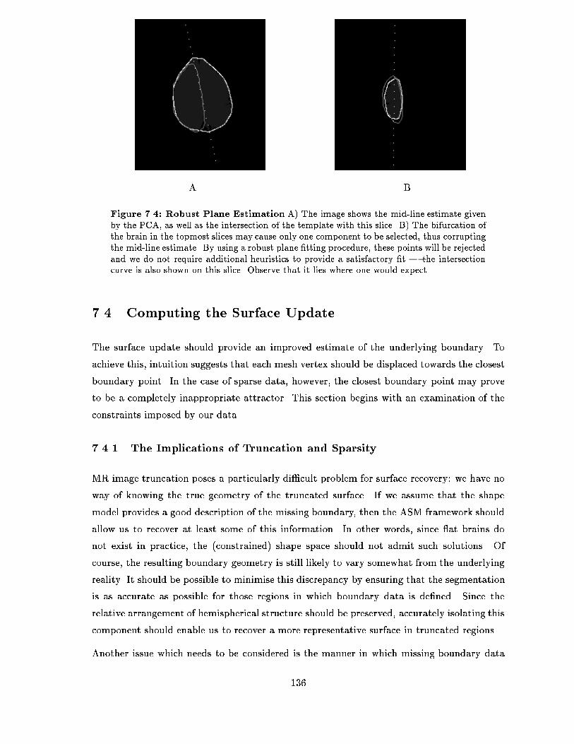
A B

Figure �� Robust Plane Estimation A� The image shows the mid�line estimate givenby the PCA� as well as the intersection of the template with this slice� B� The bifurcation ofthe brain in the topmost slices may cause only one component to be selected� thus corruptingthe mid�line estimate� By using a robust plane �tting procedure� these points will be rejectedand we do not require additional heuristics to provide a satisfactory �t � the intersectioncurve is also shown on this slice� Observe that it lies where one would expect�

�� Computing the Surface Update

The surface update should provide an improved estimate of the underlying boundary� To

achieve this� intuition suggests that each mesh vertex should be displaced towards the closest

boundary point� In the case of sparse data� however� the closest boundary point may prove

to be a completely inappropriate attractor� This section begins with an examination of the

constraints imposed by our data�

�� The Implications of Truncation and Sparsity

MR image truncation poses a particularly di�cult problem for surface recovery� we have no

way of knowing the true geometry of the truncated surface� If we assume that the shape

model provides a good description of the missing boundary� then the ASM framework should

allow us to recover at least some of this information� In other words� since �at brains do

not exist in practice� the constrained� shape space should not admit such solutions� Of

course� the resulting boundary geometry is still likely to vary somewhat from the underlying

reality� It should be possible to minimise this discrepancy by ensuring that the segmentation

is as accurate as possible for those regions in which boundary data is de�ned� Since the

relative arrangement of hemispherical structure should be preserved� accurately isolating this

component should enable us to recover a more representative surface in truncated regions�

Another issue which needs to be considered is the manner in which missing boundary data

��

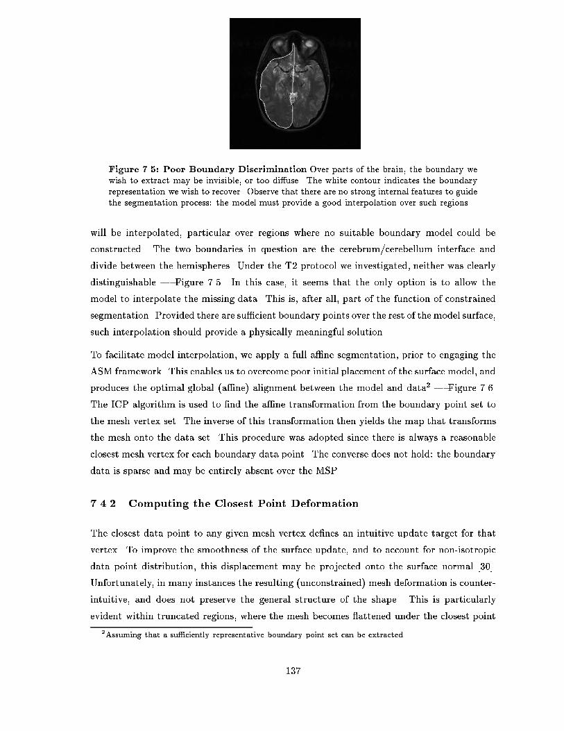
Figure �� Poor Boundary Discrimination Over parts of the brain� the boundary wewish to extract may be invisible� or too di�use� The white contour indicates the boundaryrepresentation we wish to recover� Observe that there are no strong internal features to guidethe segmentation process� the model must provide a good interpolation over such regions�

will be interpolated� particular over regions where no suitable boundary model could be

constructed� The two boundaries in question are the cerebrum�cerebellum interface and

divide between the hemispheres� Under the T� protocol we investigated� neither was clearly

distinguishable � Figure �� In this case� it seems that the only option is to allow the

model to interpolate the missing data� This is� after all� part of the function of constrained

segmentation� Provided there are su�cient boundary points over the rest of the model surface�

such interpolation should provide a physically meaningful solution�

To facilitate model interpolation� we apply a full a�ne segmentation� prior to engaging the

ASM framework� This enables us to overcome poor initial placement of the surface model� and

produces the optimal global a�ne� alignment between the model and data� � Figure ��

The ICP algorithm is used to �nd the a�ne transformation from the boundary point set to

the mesh vertex set� The inverse of this transformation then yields the map that transforms

the mesh onto the data set� This procedure was adopted since there is always a reasonable

closest mesh vertex for each boundary data point� The converse does not hold� the boundary

data is sparse and may be entirely absent over the MSP�

�� Computing the Closest Point Deformation

The closest data point to any given mesh vertex de�nes an intuitive update target for that

vertex� To improve the smoothness of the surface update� and to account for nonisotropic

data point distribution� this displacement may be projected onto the surface normal ��

Unfortunately� in many instances the resulting unconstrained� mesh deformation is counter

intuitive� and does not preserve the general structure of the shape� This is particularly

evident within truncated regions� where the mesh becomes �attened under the closest point

�Assuming that a su�ciently representative boundary point set can be extracted�

��

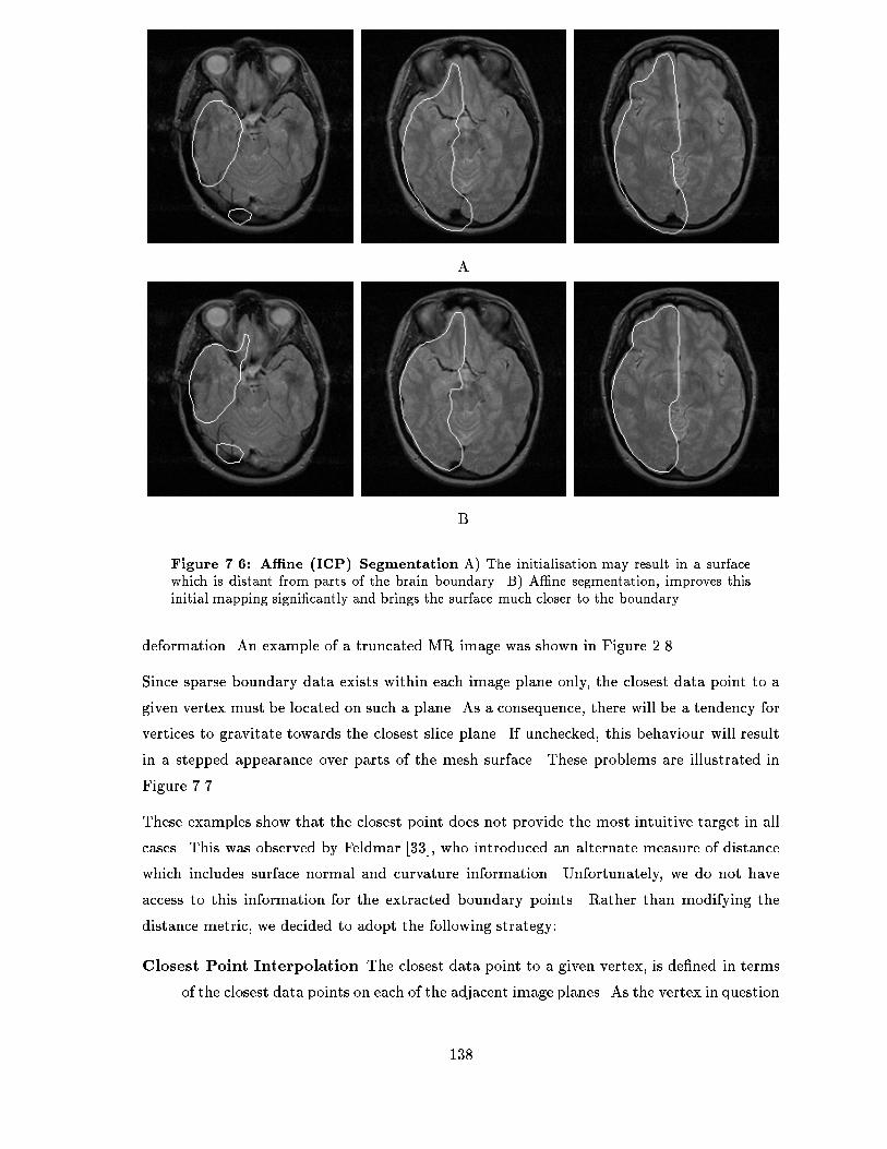
A

B

Figure �� A�ne ICP Segmentation A� The initialisation may result in a surfacewhich is distant from parts of the brain boundary� B� A�ne segmentation� improves thisinitial mapping signi�cantly and brings the surface much closer to the boundary�

deformation� An example of a truncated MR image was shown in Figure ��

Since sparse boundary data exists within each image plane only� the closest data point to a

given vertex must be located on such a plane� As a consequence� there will be a tendency for

vertices to gravitate towards the closest slice plane� If unchecked� this behaviour will result

in a stepped appearance over parts of the mesh surface� These problems are illustrated in

Figure ��

These examples show that the closest point does not provide the most intuitive target in all

cases� This was observed by Feldmar �� who introduced an alternate measure of distance

which includes surface normal and curvature information� Unfortunately� we do not have

access to this information for the extracted boundary points� Rather than modifying the

distance metric� we decided to adopt the following strategy�

Closest Point Interpolation The closest data point to a given vertex� is de�ned in terms

of the closest data points on each of the adjacent image planes� As the vertex in question

��

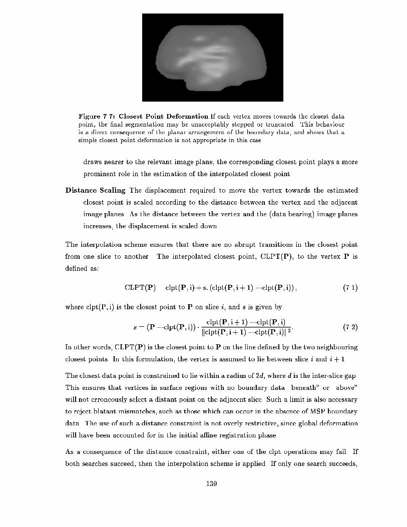
Figure �� Closest Point Deformation If each vertex moves towards the closest datapoint� the �nal segmentation may be unacceptably stepped or truncated� This behaviouris a direct consequence of the planar arrangement of the boundary data� and shows that asimple closest point deformation is not appropriate in this case�

draws nearer to the relevant image plane� the corresponding closest point plays a more

prominent role in the estimation of the interpolated closest point�

Distance Scaling The displacement required to move the vertex towards the estimated

closest point is scaled according to the distance between the vertex and the adjacent

image planes� As the distance between the vertex and the data bearing� image planes

increases� the displacement is scaled down�

The interpolation scheme ensures that there are no abrupt transitions in the closest point

from one slice to another� The interpolated closest point� CLPT P�� to the vertex P is

de�ned as�

CLPT P� � clpt P� i� s� clpt P� i �� clpt P� i��

where clpt P� i� is the closest point to P on slice i� and s is given by

s � P� clpt P� i�� clpt P� i �� clpt P� i�kclpt P� i �� clpt P� i�k� � ��

In other words� CLPT P� is the closest point to P on the line de�ned by the two neighbouring

closest points� In this formulation� the vertex is assumed to lie between slice i and i ��

The closest data point is constrained to lie within a radius of �d� where d is the interslice gap�

This ensures that vertices in surface regions with no boundary data �beneath or �above

will not erroneously select a distant point on the adjacent slice� Such a limit is also necessary

to reject blatant mismatches� such as those which can occur in the absence of MSP boundary

data� The use of such a distance constraint is not overly restrictive� since global deformation

will have been accounted for in the initial a�ne registration phase�

As a consequence of the distance constraint� either one of the clpt operations may fail� If

both searches succeed� then the interpolation scheme is applied� If only one search succeeds�

��

A B

Z

A

X

Y

Z

B

Figure �� Deformation Cusp For surface regions in which only one adjacent imageplane has data� the closest data point may switch suddenly from one side of the object tothe other as one moves across the surface� In the �gure� a cross�section of such a region isshown� along with dotted lines to indicate the e�ective closest data point for each selectedsurface point� The closest point displacement along the surface normal then results in acentral dimple� since two di�erent closest points are active�

the returned point is taken as the closest point� If both searches fail� then the vertex remains

stationary�

A linear interpolant was chosen since this method requires no higher order knowledge� such as

local curvature and requires only two data points� The shape constraints we impose encode

local curvature� and should induce the necessary adjustments to ensure that the surface

update is consistent�

In regions where only one closest point is detected� such as the top and bottom of the brain�

vertices will still move towards the closest image plane� Furthermore� if the closest point

deformation is projected onto the vertex normal� a central cusp may develop in such regions�

Figure �� This occurs because the closest point switches suddenly from one side of the closest

slice to the other� as one moves across the surface� By weighting the vertex displacement

function appropriately� we can ensures that a more natural deformation takes place� The

function we use is

W P� �

��

h� cos ��

�kPz�zck

d

�i� if kPz � zck � d

�

� otherwise� ��

where zc is the z coordinate of the closest image plane� This is a restricted form of the

equation used to moderate the data force attraction in Section ��

This weighting function is only applied when we cannot compute a closest point for both

neighbouring slices� It gradually reduces the e�ectiveness of the closest point attraction to

zero at a distance of d� from the closest slice� Vertices located beyond this point are not

attracted by the data at all� but are subject to the shape constraints� By applying these

rules� we can generate a mesh deformation which is largely in keeping with our intuition�

��

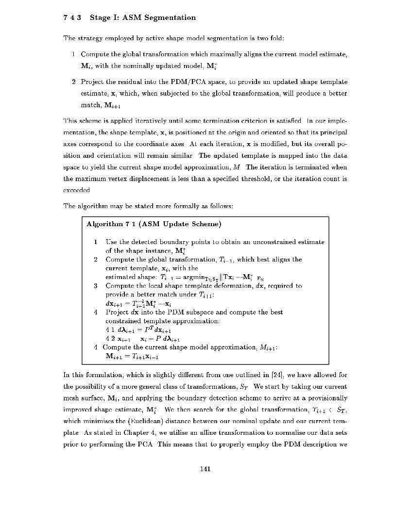
�� Stage I ASM Segmentation

The strategy employed by active shape model segmentation is twofold�

�� Compute the global transformation which maximally aligns the current model estimate�

Mi� with the nominally updated model�M�i �

�� Project the residual into the PDM�PCA space� to provide an updated shape template

estimate� x� which� when subjected to the global transformation� will produce a better

match�Mi��

This scheme is applied iteratively until some termination criterion is satis�ed� In our imple

mentation� the shape template� x� is positioned at the origin and oriented so that its principal

axes correspond to the coordinate axes� At each iteration� x is modi�ed� but its overall po

sition and orientation will remain similar� The updated template is mapped into the data

space to yield the current shape model approximation�M � The iteration is terminated when

the maximum vertex displacement is less than a speci�ed threshold� or the iteration count is

exceeded�

The algorithm may be stated more formally as follows�

Algorithm � � �ASM Update Scheme�

�� Use the detected boundary points to obtain an unconstrained estimateof the shape instance�M�

i �� Compute the global transformation� Ti�� which best aligns the

current template� xi� with theestimated shape� Ti�� argminT�STkTxi �M�

i kEN�� Compute the local shape template deformation� dx� required to

provide a better match under Ti��

dxi�� T��i��M�i � xi

�� Project dx into the PDM subspace and compute the bestconstrained template approximation�� d�i�� PTdxi�� xi�� xi P d�i��

�� Compute the current shape model approximation�Mi��Mi�� Ti��xi��

In this formulation� which is slightly di�erent from one outlined in �� we have allowed for

the possibility of a more general class of transformations� ST � We start by taking our current

mesh surface� Mi� and applying the boundary detection scheme to arrive at a provisionally

improved shape estimate� M�i � We then search for the global transformation� Ti�� ST �

which minimises the Euclidean� distance between our nominal update and our current tem

plate� As stated in Chapter �� we utilise an a�ne transformation to normalise our data sets

prior to performing the PCA� This means that to properly employ the PDM description we

��

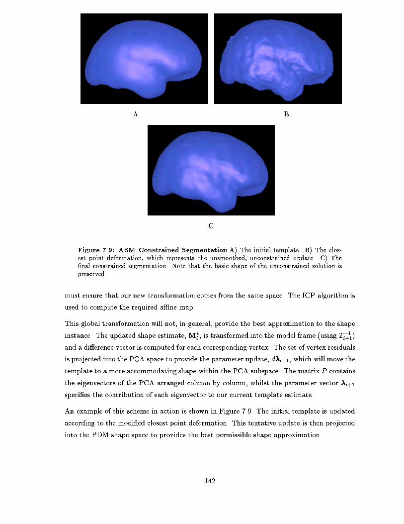
A B

C

Figure �� ASM Constrained Segmentation A� The initial template� B� The clos�est point deformation� which represents the unsmoothed� unconstrained update� C� The�nal constrained segmentation� Note that the basic shape of the unconstrained solution ispreserved�

must ensure that our new transformation comes from the same space� The ICP algorithm is

used to compute the required a�ne map�

This global transformation will not� in general� provide the best approximation to the shape

instance� The updated shape estimate�M�i � is transformed into the model frame using T

��i��

and a di�erence vector is computed for each corresponding vertex� The set of vertex residuals

is projected into the PCA space to provide the parameter update� d�i�� which will move the

template to a more accommodating shape within the PCA subspace� The matrix P contains

the eigenvectors of the PCA arranged column by column� whilst the parameter vector �i��

speci�es the contribution of each eigenvector to our current template estimate�

An example of this scheme in action is shown in Figure �� The initial template is updated

according to the modi�ed closest point deformation� This tentative update is then projected

into the PDM shape space to provides the best permissible shape approximation�

��

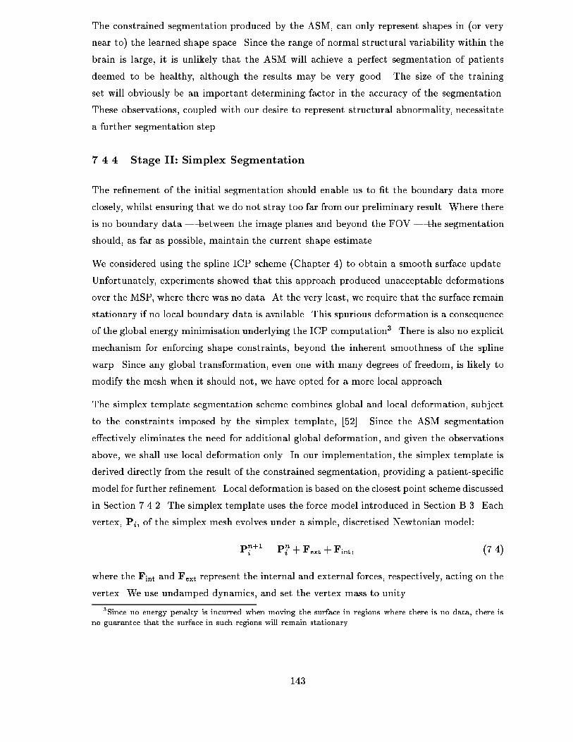
The constrained segmentation produced by the ASM� can only represent shapes in or very

near to� the learned shape space� Since the range of normal structural variability within the

brain is large� it is unlikely that the ASM will achieve a perfect segmentation of patients

deemed to be healthy� although the results may be very good� The size of the training

set will obviously be an important determining factor in the accuracy of the segmentation�

These observations� coupled with our desire to represent structural abnormality� necessitate

a further segmentation step�

�� Stage II Simplex Segmentation

The re�nement of the initial segmentation should enable us to �t the boundary data more

closely� whilst ensuring that we do not stray too far from our preliminary result� Where there

is no boundary data � between the image planes and beyond the FOV � the segmentation

should� as far as possible� maintain the current shape estimate�

We considered using the spline ICP scheme Chapter �� to obtain a smooth surface update�

Unfortunately� experiments showed that this approach produced unacceptable deformations

over the MSP� where there was no data� At the very least� we require that the surface remain

stationary if no local boundary data is available� This spurious deformation is a consequence

of the global energy minimisation underlying the ICP computation�� There is also no explicit

mechanism for enforcing shape constraints� beyond the inherent smoothness of the spline

warp� Since any global transformation� even one with many degrees of freedom� is likely to

modify the mesh when it should not� we have opted for a more local approach�

The simplex template segmentation scheme combines global and local deformation� subject

to the constraints imposed by the simplex template� �� Since the ASM segmentation

e�ectively eliminates the need for additional global deformation� and given the observations

above� we shall use local deformation only� In our implementation� the simplex template is

derived directly from the result of the constrained segmentation� providing a patientspeci�c

model for further re�nement� Local deformation is based on the closest point scheme discussed

in Section �� The simplex template uses the force model introduced in Section B�� Each

vertex� Pi� of the simplex mesh evolves under a simple� discretised Newtonian model�

Pn��i � Pn

i Fext Fint� ��

where the Fint and Fext represent the internal and external forces� respectively� acting on the

vertex� We use undamped dynamics� and set the vertex mass to unity�

�Since no energy penalty is incurred when moving the surface in regions where there is no data� there is

no guarantee that the surface in such regions will remain stationary�

��

Slice i+1Slice i

1

0

Slice j+1

No DataNo Data

d

Slice j

Z

β

Figure �� External Force Decay The strength of the external force is modi�ed ac�cording to a periodic function �sinusoid� which achieves its maximumon the image plane andits minimum at the centre of the slice gap� The function varies with distance along the ac�quisition direction only� If the vertex under consideration has only one �or no� closest points�then the periodic behaviour is broken and the function does not rise above zero beyond theimage plane on which the data point is located�

The external force is given by

Fext � Pi� � Pi � CLPT Pi�� Ni�Ni� ��

where Ni is the surface normal at vertex Pi and Pi� is a function which modi�es the

strength with which the data attracts the vertex�

The internal regularising� force is based on the local simplex angle� �i�

Fint ��

� (Pi �Pi��

where (Pi is the position of the vertex using the updated value of �i� The various possibilities

by which �i can be constrained� were discussed in Section B�� In the case of the shape

constraint� one merely insists that the simplex angle at each vertex remain constant� The

appropriate simplex angle is obtained from the corresponding vertex in the simplex template�

In the absence of external forces� the mesh will eventually relax back to the template con�gu

ration� One may also introduce a scale parameter� r� which de�nes the vertex neighbourhood�

Nr Pi�� over which simplex angles should be averaged ��

(�i ��

jNr Pi�jXi�Nr

�i� ��

The parameter r speci�es the topological distance between the vertex and its neighbours�

Two vertices are a distance r away if the shortest path connecting them contains only r

edges�

In the original framework� � and were constant for the entire mesh or designated zones��

although the external force was modi�ed by a �xed inverse square decay law� In order to

reduce the number of parameters in the system� we have �xed � at unity� and only allowed

��

to vary� To deal with the special structured nature of our boundary data� we de�ne as

follows�

P� ��

�

� cos ��

kPz � zclkd

��n� � � �� n �Z� ��

This function is shown in Figure �� The function zcl P� returns the z coordinate of the

closest image plane� whilst n may be used to vary the fallo� of the interslice decay� For

vertices which have only one or no� closest point� the function is clamped to zero if the z

coordinate is located beyond the centre of the slice gap�

This function ensures that the simplex template will dominate in regions which are distant

from the boundary data� particularly at the extremities of the brain� A sinusoid was chosen

since it is naturally periodic and provides the desired decay behaviour�

By applying the simplex constraint at each step� we can ensure that a reasonable local

deformation is obtained� Points which are not in the vicinity of data � such as those on the

MSP � will remain stationary� provided the simplex averaging neighbourhood is su�ciently

local� We have used a �xed neighbourhood size� which seems to provide good results�

�� Results

Results are shown using �D visualisations as well as meshslice intersection curves� Once the

governing parameters have been set� the segmentation process is automatic� The initialisation

step may� however� require user intervention� This would be necessary if the initial a�ne map

placed the template too low down in the image volume� a possibility if the largest connected

components were incorrectly selected during bounding box estimation� In this case� one need

just use the mouse interface to translate the mesh into a better position�

�� The Template

A separate template was used for each cerebral hemisphere� The decision to use two models�

rather than a single model� was based on the intended purpose of the surfaces� laterality and

asymmetry measures� This task is facilitated if one has two surfaces in which the plane of

asymmetry is made explicit see Chapter ��

A total of �� male and female� normal controls were used to build the templates� This

number was dictated by circumstance� since only �� male� � female� subjects had been

manually segmented at the time this work was done� Control subjects were age� sex and

handedness matched to the available patient data as far as was possible�� Control subjects

�Supplied by the EC Biomorph Project

��

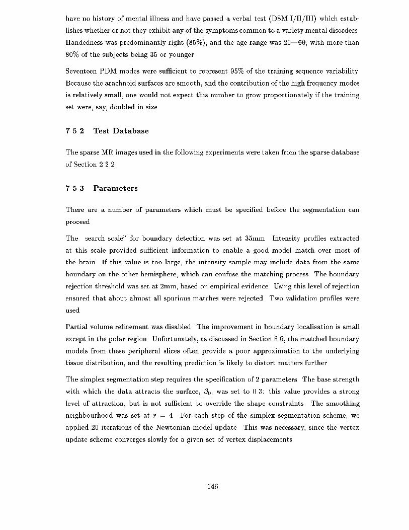
have no history of mental illness and have passed a verbal test DSM I�II�III� which estab

lishes whether or not they exhibit any of the symptoms common to a variety mental disorders�

Handedness was predominantly right ��%�� and the age range was �� with more than

��% of the subjects being �� or younger�

Seventeen PDM modes were su�cient to represent ��% of the training sequence variability�

Because the arachnoid surfaces are smooth� and the contribution of the high frequency modes

is relatively small� one would not expect this number to grow proportionately if the training

set were� say� doubled in size�

�� Test Database

The sparse MR images used in the following experiments were taken from the sparse database

of Section ��

�� Parameters

There are a number of parameters which must be speci�ed before the segmentation can

proceed�

The �search scale for boundary detection was set at ��mm� Intensity pro�les extracted

at this scale provided su�cient information to enable a good model match over most of

the brain� If this value is too large� the intensity sample may include data from the same

boundary on the other hemisphere� which can confuse the matching process� The boundary

rejection threshold was set at �mm� based on empirical evidence� Using this level of rejection

ensured that about almost all spurious matches were rejected� Two validation pro�les were

used�

Partial volume re�nement was disabled� The improvement in boundary localisation is small

except in the polar region� Unfortunately� as discussed in Section �� the matched boundary

models from these peripheral slices often provide a poor approximation to the underlying

tissue distribution� and the resulting prediction is likely to distort matters further�

The simplex segmentation step requires the speci�cation of � parameters� The base strength

with which the data attracts the surface� �� was set to �� this value provides a strong

level of attraction� but is not su�cient to override the shape constraints� The smoothing

neighbourhood was set at r � �� For each step of the simplex segmentation scheme� we

applied �� iterations of the Newtonian model update� This was necessary� since the vertex

update scheme converges slowly for a given set of vertex displacements�

��

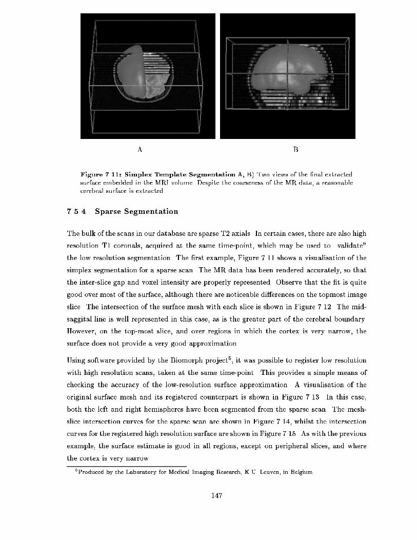
A B

Figure �� Simplex Template Segmentation A� B� Two views of the �nal extractedsurface embedded in the MRI volume� Despite the coarseness of the MR data� a reasonablecerebral surface is extracted�

�� Sparse Segmentation

The bulk of the scans in our database are sparse T� axials� In certain cases� there are also high

resolution T� coronals� acquired at the same timepoint� which may be used to �validate

the low resolution segmentation� The �rst example� Figure �� shows a visualisation of the

simplex segmentation for a sparse scan� The MR data has been rendered accurately� so that

the interslice gap and voxel intensity are properly represented� Observe that the �t is quite

good over most of the surface� although there are noticeable di�erences on the topmost image

slice� The intersection of the surface mesh with each slice is shown in Figure �� The mid

saggital line is well represented in this case� as is the greater part of the cerebral boundary�

However� on the topmost slice� and over regions in which the cortex is very narrow� the

surface does not provide a very good approximation�

Using software provided by the Biomorph project�� it was possible to register low resolution

with high resolution scans� taken at the same timepoint� This provides a simple means of

checking the accuracy of the lowresolution surface approximation� A visualisation of the

original surface mesh and its registered counterpart is shown in Figure �� In this case�

both the left and right hemispheres have been segmented from the sparse scan� The mesh

slice intersection curves for the sparse scan are shown in Figure �� whilst the intersection

curves for the registered high resolution surface are shown in Figure �� As with the previous

example� the surface estimate is good in all regions� except on peripheral slices� and where

the cortex is very narrow�

�Produced by the Laboratory for Medical Imaging Research� K�U� Leuven� in Belgium�

��

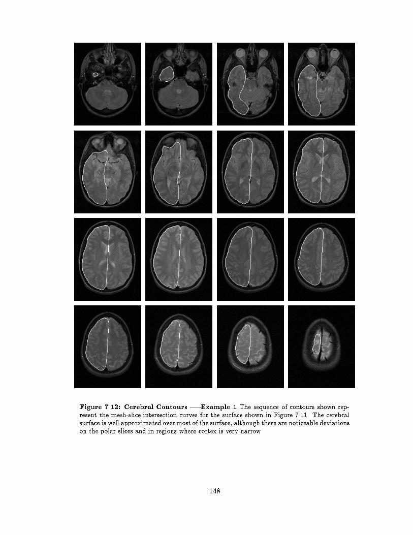
Figure �� Cerebral Contours � Example � The sequence of contours shown rep�resent the mesh�slice intersection curves for the surface shown in Figure �� The cerebralsurface is well approximated over most of the surface� although there are noticeable deviationson the polar slices and in regions where cortex is very narrow�

��

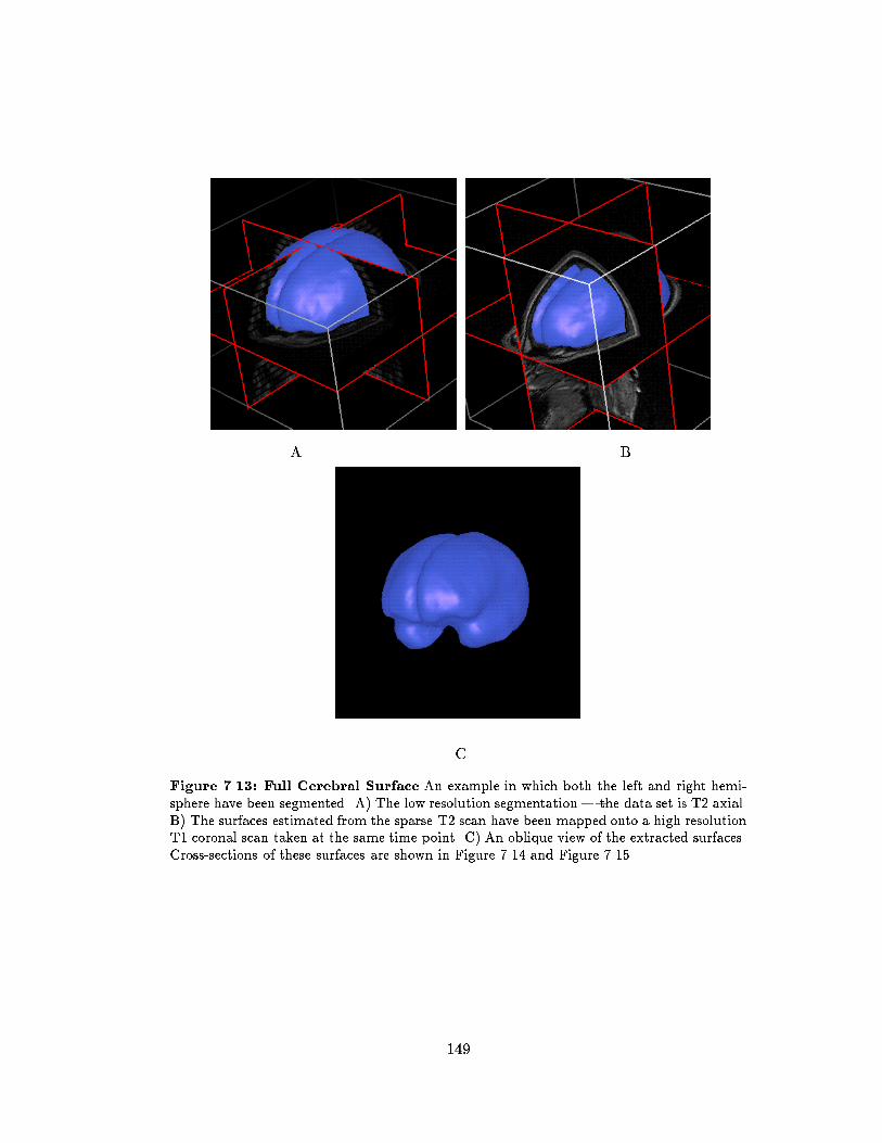
A B

C

Figure �� Full Cerebral Surface An example in which both the left and right hemi�sphere have been segmented� A� The low resolution segmentation � the data set is T� axial�B� The surfaces estimated from the sparse T� scan have been mapped onto a high resolutionT coronal scan taken at the same time�point� C� An oblique view of the extracted surfaces�Cross�sections of these surfaces are shown in Figure �� and Figure ��

��

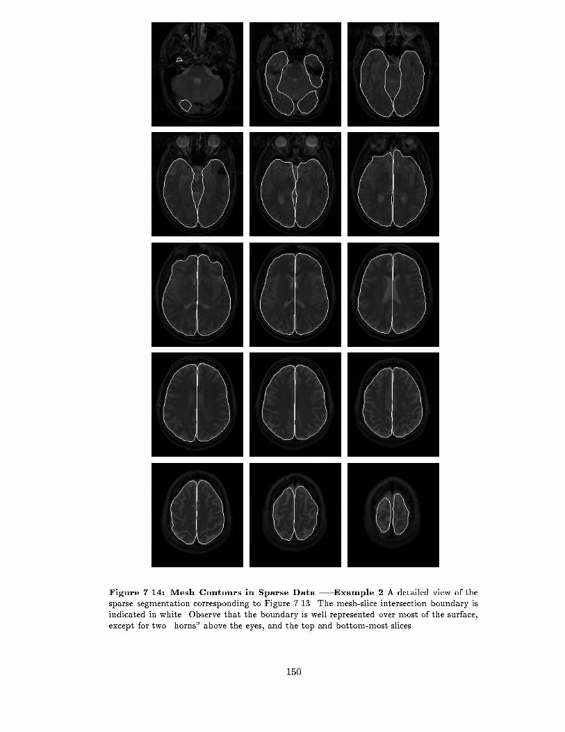
Figure �� Mesh Contours in Sparse Data � Example � A detailed view of thesparse segmentation corresponding to Figure �� The mesh�slice intersection boundary isindicated in white� Observe that the boundary is well represented over most of the surface�except for two �horns above the eyes� and the top and bottom�most slices�

��

Figure �� Mesh Contours in Dense Data � Example � This sequence of imagesshows the slice�mesh intersection curves for the transformed mesh in shown Figure ��B�Observe that the boundary provides a surface very much like the arachnoid i�e� not followingdeep sulci� The similarities between these boundary curves and those shown in Figure ��are clear� indicating that our results are consistent�

��

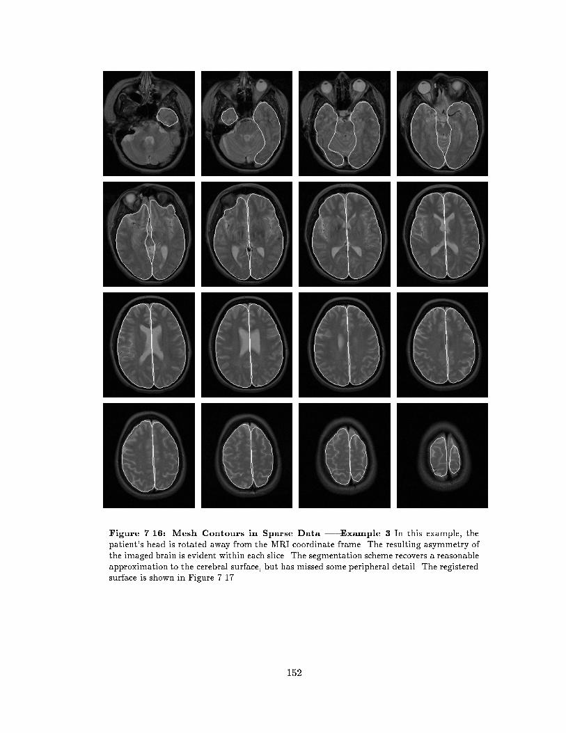
Figure �� Mesh Contours in Sparse Data � Example � In this example� thepatients head is rotated away from the MRI coordinate frame� The resulting asymmetry ofthe imaged brain is evident within each slice� The segmentation scheme recovers a reasonableapproximation to the cerebral surface� but has missed some peripheral detail� The registeredsurface is shown in Figure ��

��

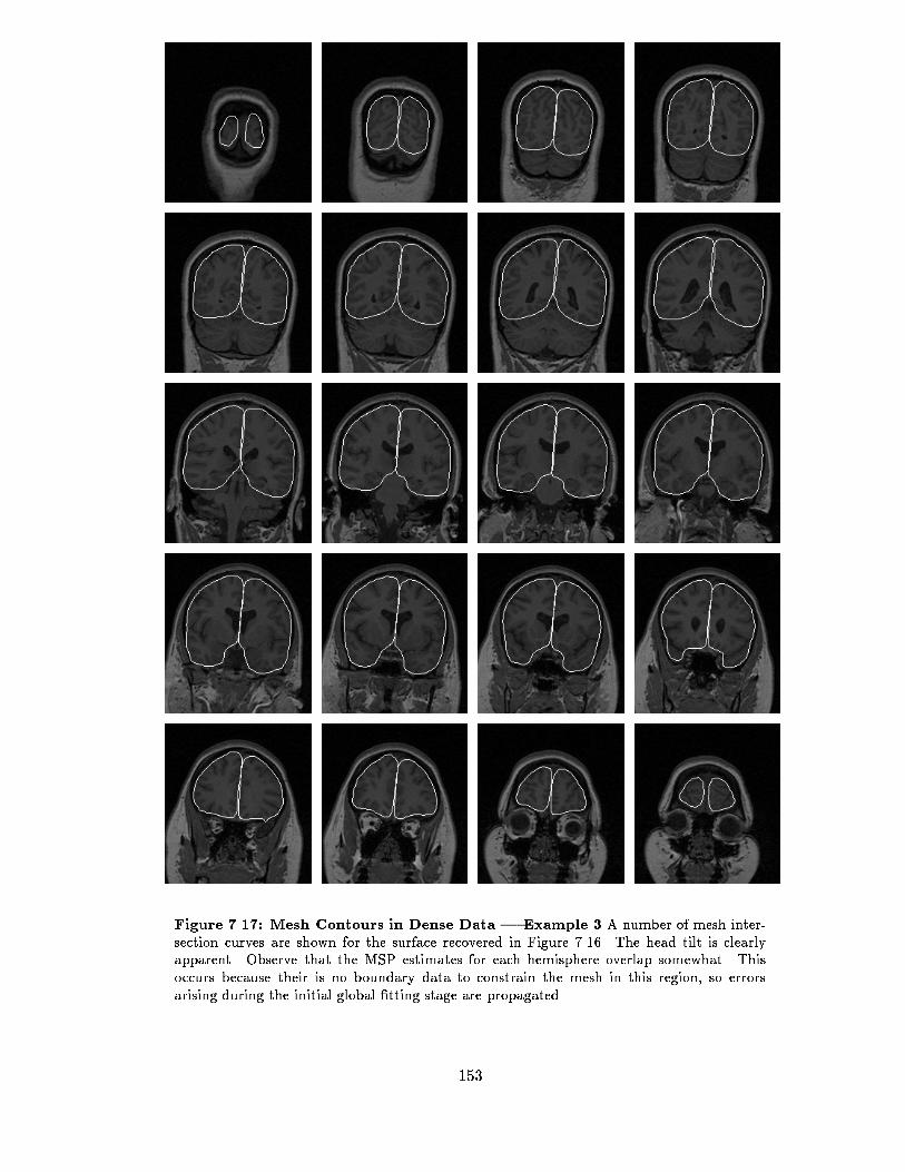
Figure �� Mesh Contours in Dense Data � Example � A number of mesh inter�section curves are shown for the surface recovered in Figure �� The head tilt is clearlyapparent� Observe that the MSP estimates for each hemisphere overlap somewhat� Thisoccurs because their is no boundary data to constrain the mesh in this region� so errorsarising during the initial global �tting stage are propagated�

��

Figure �� Mesh Contours in Sparse Data � Example � This example showsa signi�cant amount of MSP overlap� as well as tissue underestimation on the peripheralslices� Tissue underestimation is caused by a combination of boundary mismatches and themodel smoothing� The former arises mainly at the top of the brain� where CSF �lled sulcicomplicate matching� whilst the latter occurs near the base of the brain� where the cerebralcross�sections change rapidly from slice to slice�

��

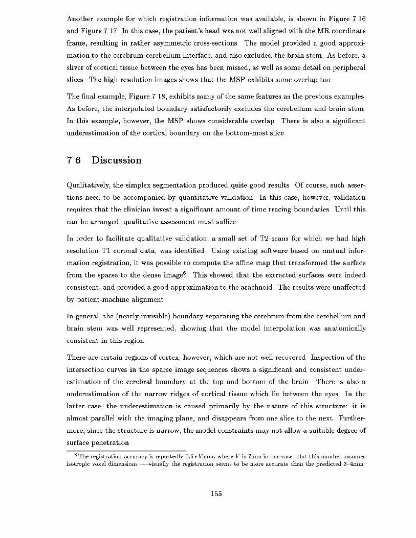
Another example for which registration information was available� is shown in Figure ��

and Figure �� In this case� the patient�s head was not well aligned with the MR coordinate

frame� resulting in rather asymmetric crosssections� The model provided a good approxi

mation to the cerebrumcerebellum interface� and also excluded the brain stem� As before� a

sliver of cortical tissue between the eyes has been missed� as well as some detail on peripheral

slices� The high resolution images shows that the MSP exhibits some overlap too�

The �nal example� Figure �� exhibits many of the same features as the previous examples�

As before� the interpolated boundary satisfactorily excludes the cerebellum and brain stem�

In this example� however� the MSP shows considerable overlap� There is also a signi�cant

underestimation of the cortical boundary on the bottommost slice�

� Discussion

Qualitatively� the simplex segmentation produced quite good results� Of course� such asser

tions need to be accompanied by quantitative validation� In this case� however� validation

requires that the clinician invest a signi�cant amount of time tracing boundaries� Until this

can be arranged� qualitative assessment must su�ce�

In order to facilitate qualitative validation� a small set of T� scans for which we had high

resolution T� coronal data� was identi�ed� Using existing software based on mutual infor

mation registration� it was possible to compute the a�ne map that transformed the surface

from the sparse to the dense image�� This showed that the extracted surfaces were indeed

consistent� and provided a good approximation to the arachnoid� The results were una�ected

by patientmachine alignment�

In general� the nearly invisible� boundary separating the cerebrum from the cerebellum and

brain stem was well represented� showing that the model interpolation was anatomically

consistent in this region�

There are certain regions of cortex� however� which are not well recovered� Inspection of the

intersection curves in the sparse image sequences shows a signi�cant and consistent under

estimation of the cerebral boundary at the top and bottom of the brain� There is also a

underestimation of the narrow ridges of cortical tissue which lie between the eyes� In the

latter case� the underestimation is caused primarily by the nature of this structure� it is

almost parallel with the imaging plane� and disappears from one slice to the next� Further

more� since the structure is narrow� the model constraints may not allow a suitable degree of

surface penetration�

�The registration accuracy is reportedly ��Vmm� where V is �mm in our case� But this number assumes

isotropic voxel dimensions � visually the registration seems to be more accurate than the predicted �mm�

��

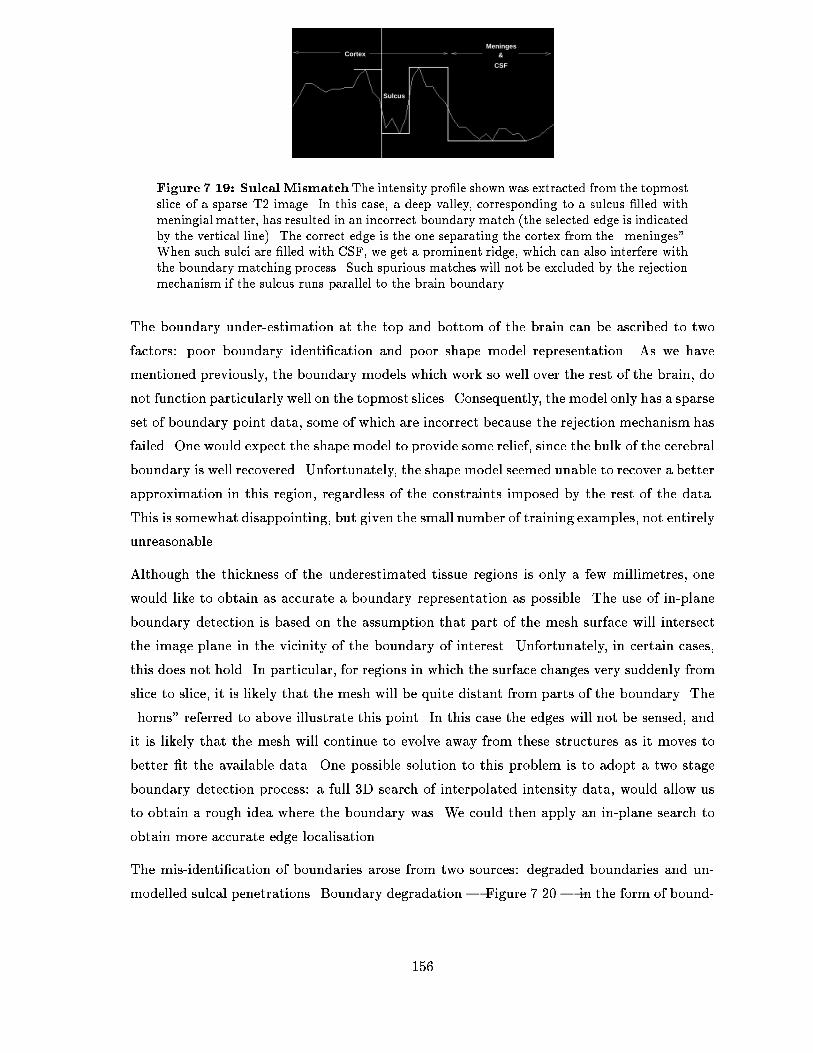
CortexMeninges

&

CSF

Sulcus

Figure �� SulcalMismatchThe intensity pro�le shown was extracted from the topmostslice of a sparse T� image� In this case� a deep valley� corresponding to a sulcus �lled withmeningial matter� has resulted in an incorrect boundary match �the selected edge is indicatedby the vertical line�� The correct edge is the one separating the cortex from the �meninges �When such sulci are �lled with CSF� we get a prominent ridge� which can also interfere withthe boundary matching process� Such spurious matches will not be excluded by the rejectionmechanism if the sulcus runs parallel to the brain boundary�

The boundary underestimation at the top and bottom of the brain can be ascribed to two

factors� poor boundary identi�cation and poor shape model representation� As we have

mentioned previously� the boundary models which work so well over the rest of the brain� do

not function particularly well on the topmost slices� Consequently� the model only has a sparse

set of boundary point data� some of which are incorrect because the rejection mechanism has

failed� One would expect the shape model to provide some relief� since the bulk of the cerebral

boundary is well recovered� Unfortunately� the shape model seemed unable to recover a better

approximation in this region� regardless of the constraints imposed by the rest of the data�

This is somewhat disappointing� but given the small number of training examples� not entirely

unreasonable�

Although the thickness of the underestimated tissue regions is only a few millimetres� one

would like to obtain as accurate a boundary representation as possible� The use of inplane

boundary detection is based on the assumption that part of the mesh surface will intersect

the image plane in the vicinity of the boundary of interest� Unfortunately� in certain cases�

this does not hold� In particular� for regions in which the surface changes very suddenly from

slice to slice� it is likely that the mesh will be quite distant from parts of the boundary� The

�horns referred to above illustrate this point� In this case the edges will not be sensed� and

it is likely that the mesh will continue to evolve away from these structures as it moves to

better �t the available data� One possible solution to this problem is to adopt a two stage

boundary detection process� a full �D search of interpolated intensity data� would allow us

to obtain a rough idea where the boundary was� We could then apply an inplane search to

obtain more accurate edge localisation�

The misidenti�cation of boundaries arose from two sources� degraded boundaries and un

modelled sulcal penetrations� Boundary degradation � Figure �� in the form of bound

��

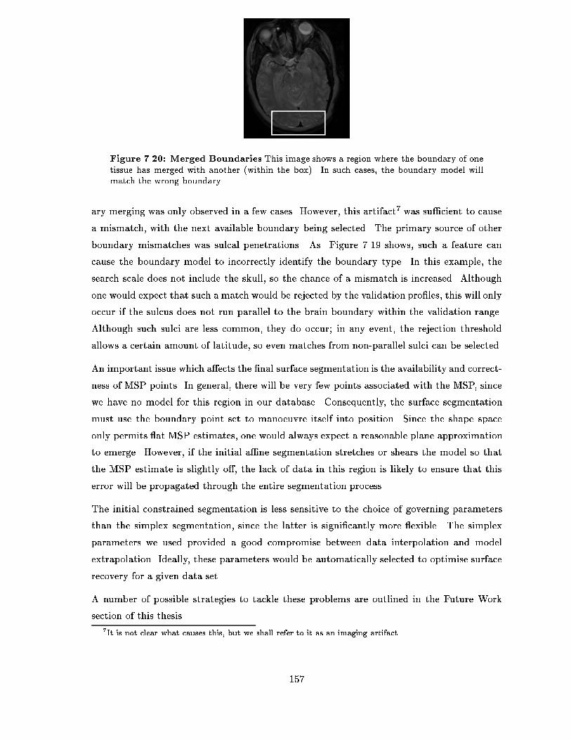
Figure �� Merged Boundaries This image shows a region where the boundary of onetissue has merged with another �within the box�� In such cases� the boundary model willmatch the wrong boundary�

ary merging was only observed in a few cases� However� this artifact was su�cient to cause

a mismatch� with the next available boundary being selected� The primary source of other

boundary mismatches was sulcal penetrations� As Figure �� shows� such a feature can

cause the boundary model to incorrectly identify the boundary type� In this example� the

search scale does not include the skull� so the chance of a mismatch is increased� Although

one would expect that such a match would be rejected by the validation pro�les� this will only

occur if the sulcus does not run parallel to the brain boundary within the validation range�

Although such sulci are less common� they do occur! in any event� the rejection threshold

allows a certain amount of latitude� so even matches from nonparallel sulci can be selected�

An important issue which a�ects the �nal surface segmentation is the availability and correct

ness of MSP points� In general� there will be very few points associated with the MSP� since

we have no model for this region in our database� Consequently� the surface segmentation

must use the boundary point set to manoeuvre itself into position� Since the shape space

only permits �at MSP estimates� one would always expect a reasonable plane approximation

to emerge� However� if the initial a�ne segmentation stretches or shears the model so that

the MSP estimate is slightly o�� the lack of data in this region is likely to ensure that this

error will be propagated through the entire segmentation process�

The initial constrained segmentation is less sensitive to the choice of governing parameters

than the simplex segmentation� since the latter is signi�cantly more �exible� The simplex

parameters we used provided a good compromise between data interpolation and model

extrapolation� Ideally� these parameters would be automatically selected to optimise surface

recovery for a given data set�

A number of possible strategies to tackle these problems are outlined in the Future Work

section of this thesis�

It is not clear what causes this� but we shall refer to it as an imaging artifact�

��

� Conclusion

In this chapter we have developed a scheme for constrained segmentation within sparse MR

data� The segmentation algorithm is based on a twotier approach� and uses boundary

data obtained from the boundary matching scheme introduced earlier� The �rst stage of

the algorithm applies learned shape constraints to produce the best segmentation permitted

within the associated shape space� The second phase uses this result as a patientspeci�c

simplex template� which loosely constrains the evolving surface and permits a more accurate

�nal solution� The method is essentially automatic� requiring no additional user intervention

after the initial speci�cation of parameters� Examples where shown for the segmentation of

the left and right cerebral hemispheres� These surfaces may be used in subsequent asymmetry

analysis�

��

Chapter

Conclusion

This thesis investigated the segmentation of the cerebral surface from sparse MRI� Sparse

images pose di�culties for many image segmentation methods� since they are poorly subsam

pled and heavily truncated� In order to overcome these problems� we have made extensive

use of a priori information� This information was primarily encapsulated in the form of two

models� a shape model and a model of the expected boundary structure�

The segmentation process consists of boundary detection followed by surface �tting� A

database of �D piecewise constant boundary models� corresponding to idealised boundary

crosssections� is speci�ed in advance� For a given �D intensity pro�le� each model is matched

in turn� and� provided the model constraints are respected� the best match is accepted� The

matching process returns the location of the associated �D boundary point� The set of bound

ary points must then be interpolated to yield a surface � but in a robust and anatomically

meaningful manner� This is achieved through the use of a shape template� The template is

generated from a representative set of apparently�� normal individuals and encodes the

permissible shape variation of the sample normal population� A simplex mesh is used to

represent the model surface� and at each iteration� the mesh vertices are adjusted to better

�t the �D boundary point set� subject to the learned shape constraints� Upon convergence�

the mesh provides the �optimal constrained segmentation for the boundary under consid

eration� To represent pathology or deformation not permitted under the model�� the shape

constraint is relaxed� A local update scheme� based on the properties of the simplex mesh� is

used� Under this constraint� the mesh smoothly evolves from the result of the initial surface

estimate� The simplex shape constraints are weak� and seek only to preserve the existing

surface geometry over regions which are far from the boundary data�

The segmentation scheme is speci�cally tailored to suit the requirements of the sparse frame

work� The boundary detection component only considers voxels within each image slice� thus

eliminating the need to consider spurious� interpolated intensity data� A method is also

developed to predict the intensity of partially �lled voxels� since these are shown to have a

��

signi�cant e�ect on boundary localisation� This is achieved by combining a simple model of

MR image formation with the matched models resulting from the boundary detection phase�

These predicted intensities are used to build a local intensity model which may be used to

re�ne the boundary estimate� The surface update is also modi�ed� the de�nition of the

closest point� which is used in both stages of the segmentation� is adapted to account for the

planar arrangement of the boundary data�

On the whole� the resulting surfaces were satisfactory� Currently� only qualitative �validation

has been performed� through the use of registered high resolution data sets� For those data

sets which did not have a high incidence of boundary degradation� the �nal surfaces provided

a good compromise between data interpolation and model extrapolation� When there were

clear discrepancies between the surface approximation and the cerebral boundary� these can

be traced to a small but recurrent set of problems which are addressed in the future work

section below�

�� Future Work

While the results presented are encouraging� there is much that can be done to improve the

accuracy of the recovered surfaces�

�� The Shape Template

The shape template was built from a training set of �� normal male and female� subjects�

Given the variability exhibited by anatomical structures� it seems likely that a larger training

set would provide a more representative constrained segmentation� Since the simplex shape

constraint is built from this initial segmentation� one would also expect an improvement in

the accuracy of the �nal extracted surface� A separate template should also be built for each

sex� since there are genderspeci�c structural di�erences which it may be useful to eliminate

from subsequent shape analysis�

�� The Boundary Model

The boundary detection process is sensitive to the choice of controlling parameters� In partic

ular� the rejection threshold may be such that valid matches are ignored because the di�erence

in the orientation of the boundary and the local surface patch is too large� In many cases�

these points become feasible as the surface updates� However� in other cases� particularly

when narrow structures are involved� the lack of data ensures that the surface will not provide

a good representation of local structure� An adaptive rejection threshold� based on the local

curvature of the template could be developed� Alternatively� a new �distance metric could

��

be introduced which included the greyscale di�erence between neighbouring pro�les as well

as the separation of the detected boundary points�

The model matching process works well in most cases� but if the boundary is severely degraded

or merges with a neighbouring tissue class� then an incorrect match may result� Since this

degradation tends to be very localised� the constrained segmentation can cope adequately�

Unfortunately� the simplex segmentation is likely to develop unwanted bumps or dimples in

such regions� The boundary model constraints play an important role in determining which

boundary points are matched� by insisting on tighter limits on model variability� this problem

can be reduced or eliminated� In particular� absolute constraints can be introduced on the

permissible length variation of each tissue interval� Such knowledge could be acquired by

consultation with neuroanatomists� for example� In this case� a spurious boundary match

would result in a unnaturally dilated or contracted tissue interval which would cause the

match to be rejected�

�� PVE Prediction

The PVE prediction scheme produced encouraging results� but was unable to much improve

boundary localisation near the top of the brain� The primary cause for this failure is the

existence of �uid�lled sulci� which produce sharp ridges or valleys in the intensity signal�

These features are su�ciently wide to ensure that simple smoothing will not remove them�

One possibility is to model these �uctuations as variable width tissue bands� although given

their arbitrariness� this may prove di�cult� Another approach would involve the preprocess

ing of the intensity pro�le� using some sort of structure preserving multiscale scheme� At

a coarse scale this would eliminate these signal �uctuations� thus enabling us to obtain an

initial boundary estimate� Once the boundary locality had been established� a small window

of the original signal intensities could be examined in order to re�ne the �t�

�� Segmenting Other Structures

The techniques developed for the cerebral surface were tested on T� and T� axial scans� Only

the cerebral hemispheres were extracted� However� the methodology we developed is suitable

for use with any structure for which we can construct a shape template and a boundary

model database� One possible candidate for study is the ventricular system� In this case the

topology is more complex� but the boundary model is fairly simple� The one component of the

segmentation scheme which will need to be adapted is the initialisation step� However� since

the initialisation may be very coarse� it should be easy enough to construct an appropriate

initialisation scheme� using� for example� thresholding�

��

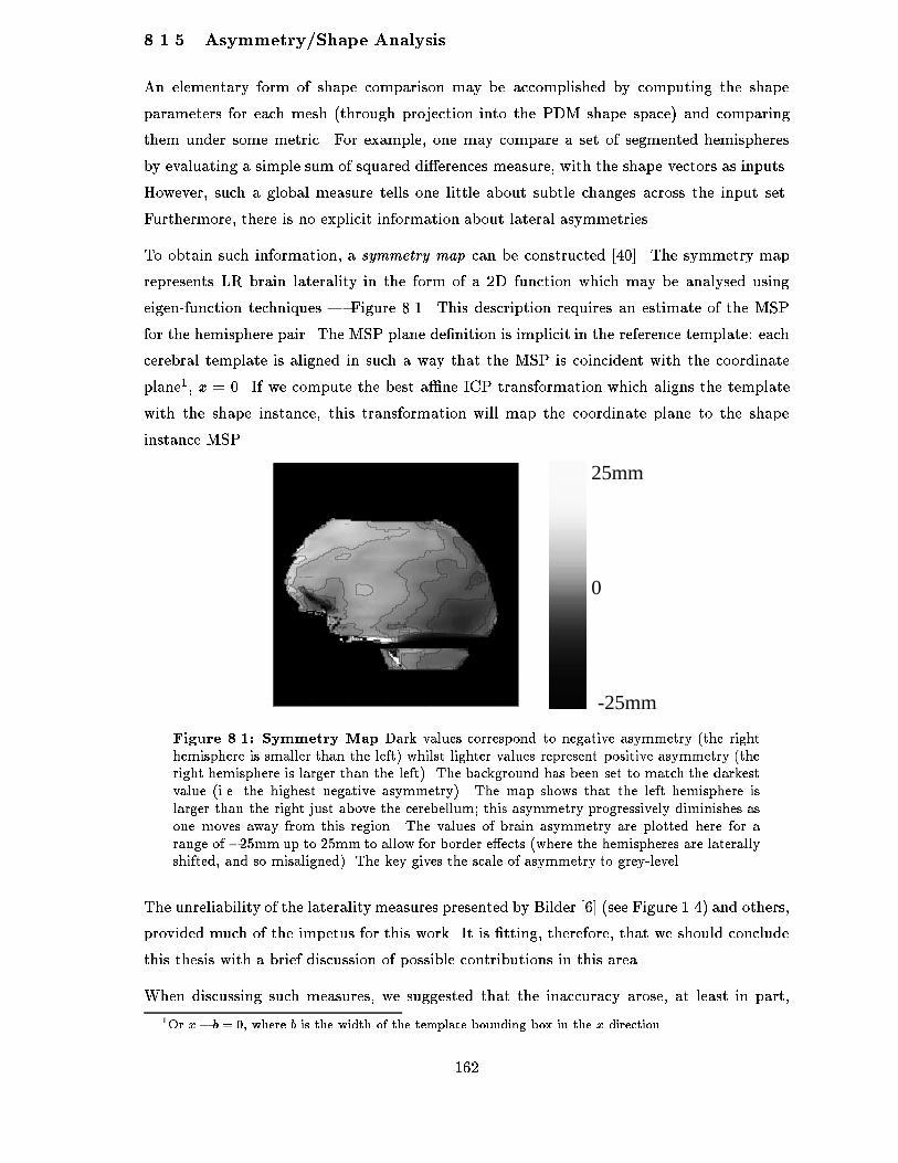
�� Asymmetry�Shape Analysis

An elementary form of shape comparison may be accomplished by computing the shape

parameters for each mesh through projection into the PDM shape space� and comparing

them under some metric� For example� one may compare a set of segmented hemispheres

by evaluating a simple sum of squared di�erences measure� with the shape vectors as inputs�

However� such a global measure tells one little about subtle changes across the input set�

Furthermore� there is no explicit information about lateral asymmetries�

To obtain such information� a symmetry map can be constructed �� The symmetry map

represents LR brain laterality in the form of a �D function which may be analysed using

eigenfunction techniques � Figure �� This description requires an estimate of the MSP

for the hemisphere pair� The MSP plane de�nition is implicit in the reference template� each

cerebral template is aligned in such a way that the MSP is coincident with the coordinate

plane�� x � �� If we compute the best a�ne ICP transformation which aligns the template

with the shape instance� this transformation will map the coordinate plane to the shape

instance MSP�

-25mm

25mm

0

Figure �� Symmetry Map Dark values correspond to negative asymmetry �the righthemisphere is smaller than the left� whilst lighter values represent positive asymmetry �theright hemisphere is larger than the left�� The background has been set to match the darkestvalue �i�e� the highest negative asymmetry�� The map shows that the left hemisphere islarger than the right just above the cerebellum� this asymmetry progressively diminishes asone moves away from this region� The values of brain asymmetry are plotted here for arange of ��mm up to ��mm to allow for border e�ects �where the hemispheres are laterallyshifted� and so misaligned�� The key gives the scale of asymmetry to grey�level�

The unreliability of the laterality measures presented by Bilder �� see Figure �� and others�

provided much of the impetus for this work� It is �tting� therefore� that we should conclude

this thesis with a brief discussion of possible contributions in this area�

When discussing such measures� we suggested that the inaccuracy arose� at least in part�

�Or x� b � � where b is the width of the template bounding box in the x direction�

��

from the sparsity of the data and the use of voxelbased segmentations� Based on the results

presented earlier� it seems clear that a signi�cant improvement in accuracy could be achieved

if the sparse segmentation framework was adopted� Dense laterality estimates symmetry

maps� may be obtained using the scheme suggested above� If the brains are registered to a

canonical reference brain� as suggested in �� one can generate a normalised set of laterality

measures� and produce a graph similar to that shown in Figure �� Because of the improved

surface correspondence arising from registration and more accurate boundary localisation�

one would expect a marked decrease in the width of the error bars� Such an improvement is

necessary if the asymmetry hypothesis is to be investigated with any con�dence�

These various tasks constitute a signi�cant amount of additional work� but for the most part

they require only small modi�cations to the existing infrastructure�

��

Appendix A

B�Spline snakes

A�� De nition

A B�spline �� is a smooth curve which consists of polynomial segments� called spans�

joined at knot points� Within each span the curve is a weighted sum of a set of control

points� Xi� where the weighting or blending functions� denoted Bj t�� are simple polynomial

functions of a curve parameter t� For example� for a cubic Bspline function Figure A��

there are four control points per span� and four blending functions�

B� t� ��

�t��

B� t� � �� t �� t �� t ��

B� t� ��

� � t �� t �� t ��

B� t� � �� t �� t �� t ��

where t � �� Within the span the curve is given by

x t� ��X

j��

XjBj t�� A��

In general� the Bspline does not pass through the control points� which is why it is called an

approximating rather than an interpolating spline� Observe� however� that if a control point�

say Xj � is moved� say to become Xj T� then equation A�� shows that the spline will be

pulled in the same direction T by an amount that is determined by the set of weights Bj t��

��

Figure A�� Cubic B spline The control points de�ne the spline� By moving them� onecan adjust the position of the curve�

Usually there are more than four control points� in which case the control points are ordered

and the spans are determined by consecutive sets of d � control points� where d is the degree

of the polynomial� For a closed curve the number of spans is equal to the number of control

points�

Generally� if there is a set of spans� the curve on each span is given by

xi t� ��X

j��

XjBi�j t�� A��

where the range of the parameter t is broken up into unit length intervals� one for each span�

The index i in the expression above indicates the ith parameter span which will have a

value determined at each point by the weighted sum of the Bi�j t�� Note that in general

the blending functions may vary from span to span� in particular they tend to be di�erent

in spans near the end of the curve� in order to ensure that the endpoints are interpolated

correctly� This is why Equation A�� uses the notation Bi�j t�� In fact� this subtlety is not

necessary in the work presented here� if the initial and �nal control points of the curve are

the same� i�e� X �� X N�� then it can be shown that the set of weight functions Bi�j t� is

the same for each span�

The degree of the spline used determines the order of continuity along the curve� In the

case of a cubic spline derivatives up to second order curvature� are continuous� A quadratic

spline requires only three control points per span� but is continuous only up to �rst derivative

tangency�� and the curvature is piecewise constant along the curve�

��

The spline equations are generally rewritten to make them amenable to standard matrix

manipulations� For general degree d� we have�

xi t� � �� t� � � � � td �BiSi

�B�

X��Xl

�CA A��

where � � t � �� The expression for yi t� is similar� but with Yi substituted for Xi�

The matrix Bi provides the Bspline coe�cients for the ith span the coe�cients of the

blending functions� while Si selects the appropriate control points for the same span � it�s

just a matrix with ones for each control point to be selected and zeros elsewhere� Span j

requires control points indexed by j�d� � � � � j� �� j� If the spline is closed� this is simply theindex modulo the number of control points�

In the following the snakes used are closed� and the matrix Bi is the same for all spans� For

example� the cubic Bspline matrix cf� Equation A�� is

B ��

�

�BB��

�CCA A��

The number of control points determines the range of the spline parameter� For M control

points� the parameter s has range ��M �� if the spline is closed! ��M � d�� if the spline is

open�

A�� Area measurements

For a closed parameterized plane curve� Green�s Theorem can be used to to compute the

enclosed area as a onedimensional contour integral� For a spline which has� say� M control

points� and consequently� M spans�� the expression reduces to

Area �M��Xn��

Z �

�xn s� *yn s� ds A��

where *yn s� denotes the derivative of yn with respect to s� Given the spline de�nitions above�

this may be rewritten as

Area �M��Xn��

dXi��

dXj��

X�n�i�MY�n�j�MHij � A��

��

in which� n � i�%M means modulo M � since the curve is closed and the M ��st point

identi�ed with the �rst! the matrix is given by H

Hij �

Z �

�Bi t� *Bj t�dt� A��

where Bl t� are the Bspline blending functions we referred to earlier� For example� in the

cubic case� we �nd

H �

�BB�

� �

��

� � � ��

� ��

��

��

��

��

� � � ��

� ��

��

��

�CCA A��

Because the spline is closed� the Bl t� are independent of the span� and the matrix is the

same for all spans� The summation over i and j only considers the relevant control points

points for each span� i�e�� the explicit Si matrix is not necessary�

��

Appendix B

The Simplex Mesh Formalism

A Simplex Mesh is a set of connected vertices which possess �xed vertex connectivity� More

formally� a k�Simplex Mesh� M of Rd� is de�ned by the pair V M�� N M�� where V M�

is the vertex set and N M� provides the vertex connectivity mapping� For this work� d � �

and k � � surface in �D�� Since our work will concern �simplex surface� meshes only� we

shall focus on them and drop the explicit k pre�x unless we wish to state a more general

result�

The vertex connectivity mapping ensures that

�� each vertex is connected to k � other vertices

�� there are no cycles or loops in the edge representation�

A mesh with these properties is so named because the set of points directly connected to any

given vertex comprises a ksimplex� according to the following de�nition�

De�nition B � �k�simplex� A k�simplex of Rd� k � d� is a set of k � independent

points in Rd

For example� in a �simplex surface� mesh� each vertex is directly linked to three neighbours�

which comprise the local simplex in R�� Since the mesh is not degenerate� the � neighbouring

points are independent� as required by the de�nition�

There is a close relationship between the simplex mesh and a triangulation of the vertex set�

as suggested by the usage of the term �simplex� They are in fact dual representations i�e� we

can derive one from the other � Figure B��a�� This duality is topological� the simplex mesh

and its associated dual triangulation need not be geometrically equivalent� in the sense that

the �dual of the dual will not� in general� result in the original simplex mesh or triangulation�

This may be formally proved by examining the Euler equations relating the number of vertices�

edges and faces in each representation� One can� however� establish geometric equivalence

between a simplex mesh with planar polygons and its dual triangulation� Although there

��

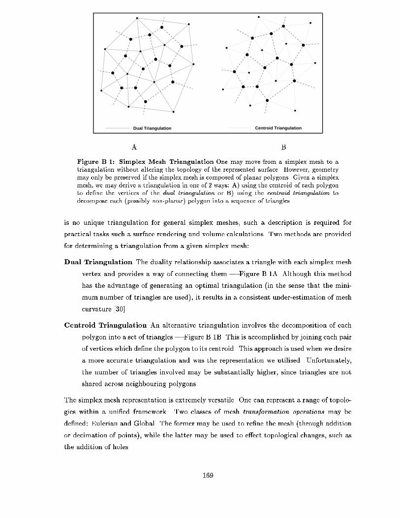
Centroid TriangulationDual Triangulation

A B

Figure B�� Simplex Mesh Triangulation One may move from a simplex mesh to atriangulation without altering the topology of the represented surface� However� geometrymay only be preserved if the simplex mesh is composed of planar polygons� Given a simplexmesh� we may derive a triangulation in one of � ways� A� using the centroid of each polygonto de�ne the vertices of the dual triangulation or B� using the centroid triangulation todecompose each �possibly non�planar� polygon into a sequence of triangles�

is no unique triangulation for general simplex meshes� such a description is required for

practical tasks such a surface rendering and volume calculations� Two methods are provided

for determining a triangulation from a given simplex mesh�

Dual Triangulation The duality relationship associates a triangle with each simplex mesh

vertex and provides a way of connecting them � Figure B��A� Although this method

has the advantage of generating an optimal triangulation in the sense that the mini

mum number of triangles are used�� it results in a consistent underestimation of mesh

curvature ��

Centroid Triangulation An alternative triangulation involves the decomposition of each

polygon into a set of triangles � Figure B��B� This is accomplished by joining each pair

of vertices which de�ne the polygon to its centroid� This approach is used when we desire

a more accurate triangulation and was the representation we utilised� Unfortunately�

the number of triangles involved may be substantially higher� since triangles are not

shared across neighbouring polygons�

The simplex mesh representation is extremely versatile� One can represent a range of topolo

gies within a uni�ed framework� Two classes of mesh transformation operations may be

de�ned� Eulerian and Global� The former may be used to re�ne the mesh through addition

or decimation of points�� while the latter may be used to e�ect topological changes� such as

the addition of holes�

��

i

ri

O

N

i

i

S

S

1

2

R

P

C i

i

3PN (i)1

N (i)

PN (i)2

P

Figure B�� Simplex Angle The simplex angle at a mesh vertex� Pi� provides a measureof local deviation from a plane viz� the one de�ned by the three neighbouring mesh vertices� PN��i�� PN��i�� PN��i�� The circle� S�� passing through these three points has radius ri andcentre Ci� while the sphere� S�� which passes through all four points has radius Ri and iscentred at Oi� The simplex angle is independent of the position of the neighbouring pointson the S� and is zero when Pi is on the plane de�ned by these points�

B�� Geometric Properties

At each vertex� Pi on an oriented� simplex mesh� one may de�ne a normal vector using the

plane passing through the � neighbouring points� PN��i� PN��i� PN��i��

Ni �PN��i � PN��i PN��i � PN��i PN��i � PN��i

kPN��i � PN��i PN��i � PN��i PN��i � PN��ik B��

A given vertex together with its � neighbours de�nes a tetrahedral mesh element� Given these

points� one may compute a quantity known as the simplex angle� which provides a means of

quantifying the local discrete curvature about the vertex�

De�nition B � �Simplex Angle� Let S� be the circumscribed circle at the three neighbour�

ing mesh vertices PN��i� PN��i� PN��i� This circle has radius ri and centre Ci Let S� be

the circumscribed sphere at the four vertices Pi� PN��i� PN��i� PN��i�� with associated origin

Oi and radius Ri �See Figure B� The simplex angle� �i� at vertex Pi is de�ned by

sin �i� �ri

Ri

� sgn �� PiPN��i �Ni�

cos �i� �kOiCikRi

� sgn �� OiCi �Ni� B��

Here kOiCik represents the distance from the centre of the sphere to the plane and �i �� sgn�x� returns � depending on the sign of its argument

��

iF

3

N (i)P

iP

1

N (i)P

2N (i)P

Figure B�� Metric Parameters The orthogonal projection� Fi� of the vertex Pi onto theplane passing through its � neighbours may be described through � metric parameters �for a��simplex mesh�� Only � need be speci�ed since they must collectively sum to unity� Theseparameters provide �barycentric coordinates for the projected point and o�er a meansof enforcing some local regularity on the mesh� we require that these parameters alwaysbe positive� This precludes the existence of skewed mesh elements and is a form of localregularisation�

The simplex angle is independent of the positions of the points PN��i� PN��i� PN��i� on the

circle S� and of the position of Pi on the circumscribed hemisphere of S�� Furthermore� it is

zero only when Pi lies on the plane de�ned by its � neighbours�

B�� Metric Parameters

In order to characterise the local geometry on a simplex mesh� a set of metric parameters�

�i � f��i� ��i� ��ig� are introduced at each vertex� These parameters describe how each vertexis placed with respect to its � neighbours� The orthogonal projection of Pi onto the plane

spanned by its � neighbours produces� Fi � Figure B�� which may be computed as

Fi � ��iPN��i ��iPN��i ��iPN��i� B��

where ��i ��i ��i � ��

The point Pi may then be represented as

Pi � Fi L ri� di� �i�Ni� B��

where ri and Ni have their previous meanings and di is the distance between Fi and the

centre of the circumscribed circle� Ci� The function L ��

L ri� di� �i� � r�i � d�i � tan�i

�qr�i r

�i � d�i � tan

� �i ri

� � � if j�ij � �

�

� � �� if j�ij � �

��

B��

provides the height of the point above the plane and is primarily a means of expressing the

in�uence of the simplex angle�

��

The metric parameters provide a �barycentric description of the projected point� These

parameters are constrained to be positive in order to increase mesh stability� In practice

this does not limit the usefulness of this description �� The metric parameters together

with the simplex angle provide a unique description of a shape� up to a similarity� Since we

have no intention of representing the mesh using these parameters� this observation is of no

importance to us�

The computation of metric parameters is simple�

We have

��iPN��i ��iPN��i �� i � ��i�PN��i � Fi� B��

which leads directly to

��i PN��i � PN��i� � PN��i � PN��i�

kPN��i � PN��ik� ��i �

Fi � PN��i� � PN��i � PN��i�

k PN��i � PN��ik�� B��

and

��i ��i PN��i � PN��i� � PN��i � PN��i�

kPN��i � PN��ik�� Fi � PN��i� � PN��i � PN��i�

k PN��i � PN��ik�� B��

These equations are easily inverted� We may obtain the orthogonal projection of Fi as

Fi � Pi � Pi � PN��i�Ni� B��

where the sign of the second term assumes that the normal is direct towards Pi�

B�� The Simplex Mesh and Segmentation

The simplexmesh formalismoutlined in �� has a number of strategies for controlling smooth

ness and shape� The mesh update is

based on a Newtonian force model� Speci�cally� the movement of each node is governed by

the following di�erential equation

md�Pi

dt�� dPi

dt Fint Fext B��

where m is the mass of the node unity will be assumed� and � is a damping coe�cient� Each

node is subjected to an internal force� Fint� which express intrinsic bending constraints� and

an external force� Fext� which represents the in�uence of attractors in the environment� The

equations of motion are discretised in time as

P t��i � �� P t

i � P t��i � P t

i Fint t� Fext t�� B��

��

B�� Internal Forces

The internal forces are expressed in terms of socalled �shape functionals which characterise

the shape of the local tetrahedral element surrounding each vertex� Each element has a

rest shape� which it naturally adopts when no external stresses are applied� In this state� it

possesses a simplex angle� ��i � If we assume that the vertex Pi occupies the position P�i when

in this state� then the energy� Si� of the local tetrahedron may be as expressed as

Si � �i

�jP �i � Pij�� B��

where � � �i � �� may be used to increase the strength of the internal force in the updateequation� This value must be less than �� to ensure stability�

Under this scheme� the gradient of this energy de�nes Fint�

Fint ��Si�Pi

� �i P�i � Pi�� B��

This de�nition is consistent with an �elastic model of internal force� Combining Equa

tions B��B�� and B�� we arrive at the �nal form of Fint�

Fint � �i ��i PN��i � Pi� ��i PN��i � Pi� ��i PN��i � Pi� L ri� di� ��i �Ni�� B��

where ��i determines the particular type of mesh constraint to be enforced� Four are identi�ed�

� Null Constraint ��i � �i� This is not really a constraint � the surface can bend freely

around Pi�

� Smoothing ��i � �� Under this constraint the mesh vertices will tend to smooth the

surface regardless of local curvature of geometry�

� Mean curvature continuity

��i � arcsin

�� X

j�Nr�Pi

eij � ri � sin�jrj

�A

Xj�Nr�Pi

eij � �� eij � �� B��

where N r Pi� represents a neighbourhood of size r about Pi� This constraint smoothes

curvature and is controlled through the parameter r�

� Shape If we set ��i � ��i we can provide a �template which represents the shape to

which the mesh will revert when all external forces are removed�

In the absence of external forces� the smoothing constraint will cause the mesh to shrink in

on itself� unless the simplex mesh is a planar object� in which case ��i � � is already satis�ed�

��

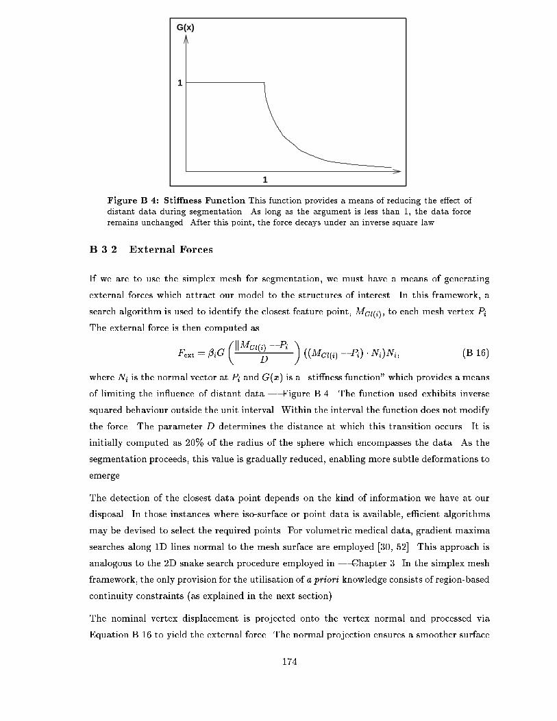
1

1

G(x)

Figure B�� Sti�ness Function This function provides a means of reducing the e�ect ofdistant data during segmentation� As long as the argument is less than � the data forceremains unchanged� After this point� the force decays under an inverse square law�

B�� External Forces

If we are to use the simplex mesh for segmentation� we must have a means of generating

external forces which attract our model to the structures of interest� In this framework� a

search algorithm is used to identify the closest feature point� MCl�i� to each mesh vertex Pi�

The external force is then computed as

Fext � iG

kMCl�i � PikD

� MCl�i � Pi� �Ni�Ni� B��

where Ni is the normal vector at Pi and G x� is a �sti�ness function which provides a means

of limiting the in�uence of distant data � Figure B�� The function used exhibits inverse

squared behaviour outside the unit interval� Within the interval the function does not modify

the force� The parameter D determines the distance at which this transition occurs� It is

initially computed as ��% of the radius of the sphere which encompasses the data� As the

segmentation proceeds� this value is gradually reduced� enabling more subtle deformations to

emerge�

The detection of the closest data point depends on the kind of information we have at our

disposal� In those instances where isosurface or point data is available� e�cient algorithms

may be devised to select the required points� For volumetric medical data� gradient maxima

searches along �D lines normal to the mesh surface are employed �� This approach is

analogous to the �D snake search procedure employed in � Chapter �� In the simplex mesh

framework� the only provision for the utilisation of a priori knowledge consists of regionbased

continuity constraints as explained in the next section��

The nominal vertex displacement is projected onto the vertex normal and processed via

Equation B�� to yield the external force� The normal projection ensures a smoother surface

��

update� particularly when sparse point data is being processed� By modifying the parameter

i the relative importance of the external force in the update equations can be controlled�

��

Appendix C

Mesh Measures

The volume and surface area of a closed� nonintersecting triangulated surface are easily

calculated�

C�� Surface Area

The surface area is simply the sum of the individual surface areas contributed by each of the

NT triangles� More speci�cally�

S �

NTXi��

k xi�� xi�� xi�� xi��k�

where xi�j� j � �� is the j vertex on the ith triangle�

C�� Volume

Gauss�s Divergence Theorem shows that we may compute the volume enclosed by any piece

wise smooth surface by evaluating the following surface integral�

V ��

�

Z ZS

x � n dS�

where n is the surface normal at x�

In the case of a nonintersecting triangular mesh� we have a surface� f�NT

i��Tig� Each Ti is atriangular facet� with a constant normal� ni� The plane spanned by this triangle is given by

x� xi�� ni � �

We are now in a position to evaluate the surface integral�

��

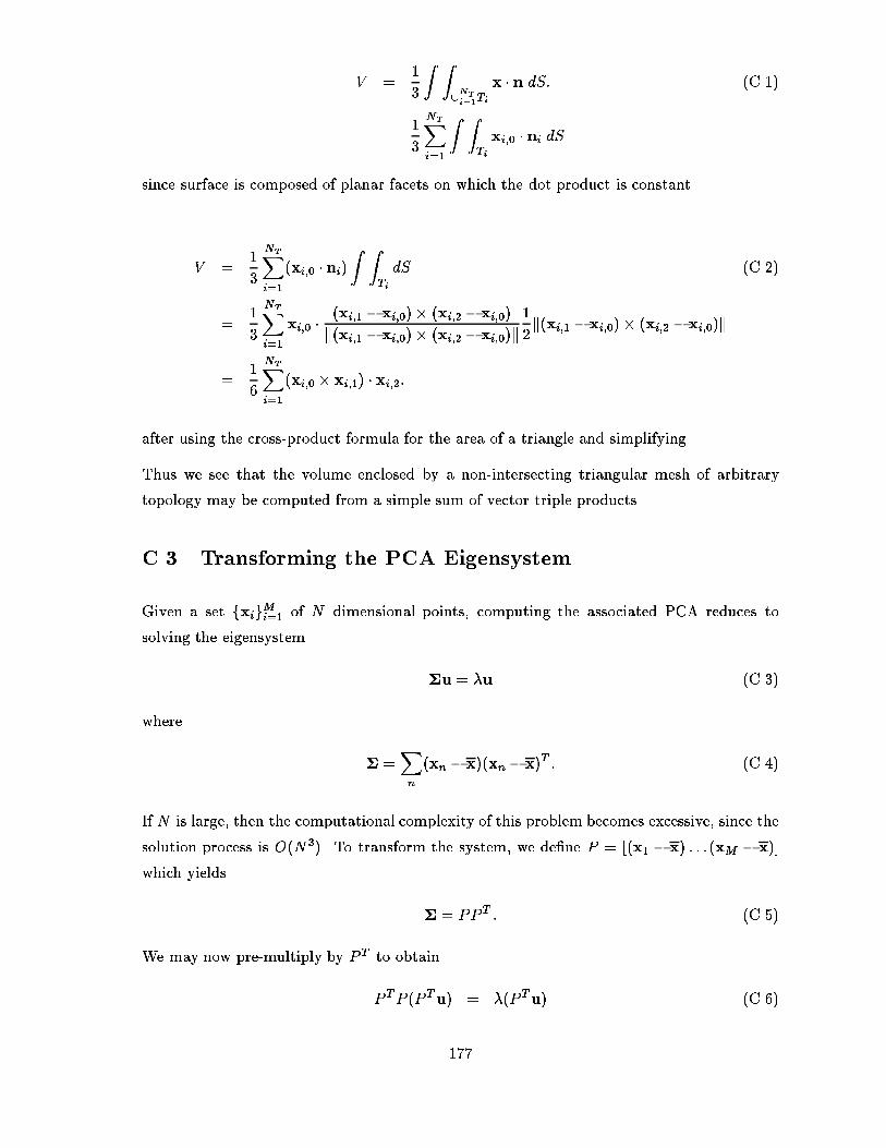
V ��

�

Z Z�NTi�Ti

x � n dS� C��

��

�

NTXi��

Z ZTi

xi�� ni dS

since surface is composed of planar facets on which the dot product is constant�

V ��

�

NTXi��

xi�� ni�Z Z

Ti

dS C��

��

�

NTXi��

xi�� xi�� xi�� xi�� xi��

k xi�� xi�� xi�� xi��k�

�k xi�� xi�� xi�� xi��k

��

�

NTXi��

xi�� xi�� xi��

after using the crossproduct formula for the area of a triangle and simplifying�

Thus we see that the volume enclosed by a nonintersecting triangular mesh of arbitrary

topology may be computed from a simple sum of vector triple products�

C�� Transforming the PCA Eigensystem

Given a set fxigMi�� of N dimensional points� computing the associated PCA reduces to

solving the eigensystem

�u � u C��

where

� �Xn

xn � x� xn � x�T � C��

If N is large� then the computational complexity of this problem becomes excessive� since the

solution process is O N�� To transform the system� we de�ne P � � x� � x� � � � xM � x��

which yields

� � PPT � C��

We may now premultiply by PT to obtain

PTP PTu� � PTu� C��

��

which is equivalent to solving the eigensystem &�v � v where &� � PTP and v � PTu�

The set of eigenvectors obtained from this system may be �interpolated to yield the eigen

vectors of Equation C�� by premultiplying each with P � The eigenvalues will be the same in

both cases�

The rank of the covariance matrix determines the number of principal components eigen

vectors� which can be determined� If the number of training examples is not equal to the

N � then the covariance matrix will be rank de�cient for one of the two eigensystems� We

always choose the eigensystem which has full rank the smaller of the two� and interpolate

the solution as shown above�

��

Appendix D

Mahalanobis PCA criterion

We are given anN dimensional PCA� de�ned by a mean� �� and a set ofN modes of variation�

feigi�� N � The Mahalanobis distance from the mean� is de�ned as

M x� � x� ��TS�� x� �� D��

where S�� is the inverse of the covariance matrix used to generate the eigensystem de�ning

the PCA�

Sei � iei� eiTei � �� i � �� N� D��

where the eigenvectors are ordered by eigenvalue� in descending order� An arbitrary vector�

x� may be expanded in the PCA system as

x � � Eb� D��

where E � �e� � � �eN� and b is a vector of shape parameters basis coe�cients��

Using these equations we have�

M x� � x� ��TS�� x� �� D��

� Eb�TS��Eb

� bT ��ij

j�ij�b

�NXj��

bj�

j�

In general� a reduced set of eigenmodes will be retained� and the expansion is truncated at

term l� l � N � In this case� one cannot compute the basis coe�cients� bi� for i � l� In ��

the eigenvalues associated with these modes are set to i ��l� i � l� This leads to

M �lX

i��

bi�

i �

l

NXi�l��

bi�� D��

��

The sum of squared di�erences� R�� between the original vector� x� and its approximation�

$x� yields�

R� � x� $x�T x� $x� D��

� E b� $b��TE b� $b�� b� $b�T b� $b�

�NXi��

bi � $bi��

�NX

i�l��

bi � $bi��

Finally� we arrive at the following�

M �lX

i��

bl�

l �R�

l D��

��

Appendix E

Cosine Foreshortening for Curved

Surfaces

Given a sequence of parallel planes� one can show that the distance between the planes scales

linearly as the angle at which the measurement is made varies� More speci�cally� if we know

the closest perpendicular� distance between two planes� then the distance measure along a

ray at an angle of � radians will be scaled by �cos � � Figure E�� This is cosine foreshortening�

We may think of this transformation as a warping of one length into another� e�ected through

some interval contraction�dilation function� w l�� where l is the distance along the sampling

line�

φ

D2

D1

Normal2

Normal1

Cosine Forseshortening

(θ)

(φ)D1 = D2 COS

L1 = L2 COS

θ = φ

normal1 = normal2

θ

L1

L2

Figure E�� Cosine foreshortening For a sequence of parallel planes� the distances be�tween any pair of planes will be linearly contracted�dilated relative to the closest �normal�distance� depending on the angle at which they are measured�

For the simple case shown in Figure E�� the warping function would be given by

w l� �l

cos �� l � �� L�� E��

��

where L is the length of the sampling line in the boundary normal direction� This rule holds

for an arbitrary number of parallel planes� all lengths will be contracted or dilated by a factor

of cos �� In this scenario� a single normal is shared by each surface�

For an arbitrary set of curved parallel surfaces� this simple behaviour only holds in a di�er

ential sense� For a �nite sampling ray� the foreshortening depends on the distance along the

ray� This follows directly from the fact that the surface normal may vary at every point on

the surface�

It is possible to derive a closed form expression for the foreshortening along such a sampling

ray� provided one is is willing to accept a compromise� By approximating the local curved

parallel surfaces by a series of concentric spheres� a simple expression may be computed�

which provides some useful insights into nature of this warping�

The construction we employ is shown in Figure E�� The sphere is assumed to be intersected

by a number of planes� representing the MR image sampling planes� The inplane sampling

lines are oriented along normals to the planesphere intersection curve which is a circle��

Because of the symmetry of the construction� we need only consider a single plane which

passes through both poles and the inplane sampling ray� This reduces the problem from �D

to simple �D plane geometry� As Figure E�� shows� the line joining each end point of the

inplane sampling ray to the sphere surface� generates two di�erent normal vectors� Since we

are only considering the situation in the plane� the normal orientation may be described by

an angle �� measured w�r�t� the sampling plane represented as a horizontal line in the �D

�gure�� Because the boundary is a circle� the normals may be linearly interpolated to give a

normal at any point between the � end points� This is equivalent to de�ning

� t� � �i t��f � �i�� t � �� E��

where �f and �i� represent the plane angles of the normals at the �nal and initial points�

respectively� of the sampling line�

One can see from the �gure that as the extent of the inplane boundary pro�le increases�

the assumption of constant normal orientation breaks down� On a small enough scale� we

can still use the constant angle assumption to generate a di�erential description of the local

foreshortening��

dl� � dl cos � l� E��

�We�re using the �inverse� foreshortening� since for most of our work we wish to transform non�normal

sampling into normal sampling�

��

θ1 θ2

θ(τ) = θ1 + τ(θ2−θ1)

Figure E�� Cosine foreshortening on the sphere By approximating a sequence ofparallel surfaces by a local spherical patch� it is possible to derive a closed form solutionfor the foreshortening along a sampling ray� In our framework� the object is intersected bya number of parallel planes� The lines along which we sample in�plane data are boundarynormals to the plane�sphere intersection curve within each slice� By considering the planewhich passes through this line and the poles of the sphere� we may reduce the problem to onewhich requires only �D planar geometry� Within this plane� the rays passing through eachend point from the sphere �circle� centre provide us with two� di�erent surface normals� Weare interested in computing the foreshortening along the in�plane sampling ray� as a functionof these delimiting angles�

To get the warping function� w l�� we can integrate over the range of � covered by surface

normals which radiate from the endpoints of our pro�le sampling line cf Figure E��

w t� �

Z t

�dl�

�

Z t

�cos � l�dl

�

Z t

�cos �i l ��f � �i��dl

�

Z t

��cos �i cos l �f � �i�� sin �i sin l �f � �i��dl

�

cos �i sin l �f � �i�

�f � �i sin �i cos l �f � �i�

�f � �i

�t�

�cos �i sin t �f � �i�

�f � �i sin �i cos t �f � �i�

�f � �i� sin �i�f � �i

� E��

The warping function is de�ned over the interval �� and speci�es the mapping from one

sampling direction to another over a normalised interval� In the de�nition of the integral

above� we used the normal line attached to �i as our standard frame� In fact� because of

the symmetry in the model� the actual warping is independent of the normal pro�le chosen

within the region delimited by our angles��

��

There are clearly regions where the model will break down� those in which the sampling

plane does not intersect the full complement of nested surfaces� This will occur at the brain

extremities� If one looks at the limiting behaviour of the warping function� we observe the

following�

lim�f��i w l� � l cos �i

lim�f��i ��i��w l� � l�

w l�j�i��

cos l��f��

�f��

�

The �rst limit tells us that as that as the normals converge� then we can revert to the standard

cosine foreshortening rule � as we would expect� In addition� as both angles tend to zero�

we recover the identity i�e� the surface normal and sampling direction coincide� When the

sampling direction and the surface normal are orthogonal � which will happen at the poles

of the sphere � then the third limit comes into play�

E�� An Example

How does warping a�ect a pro�le' Consider the example presented in Figure E��A�� The

original inplane pro�le was resampled uniformly over it�s length� which was normalised to

unity� before undergoing the warping� The delimiting normals made angles of �� and ��

radians� respectively� with the sample plane� The pro�le was warped onto the surface normal

passing through the �rst end point although it could equally well have been applied to the

second point��

For comparison� a direct cosine warp is shown� with the foreshortening angle being taken as

the average of the angles subtended by the end point normals� Note the signi�cant di�erence

in the peak separation! the nonlinearities are more subtle � cf� Figure E��B��

��

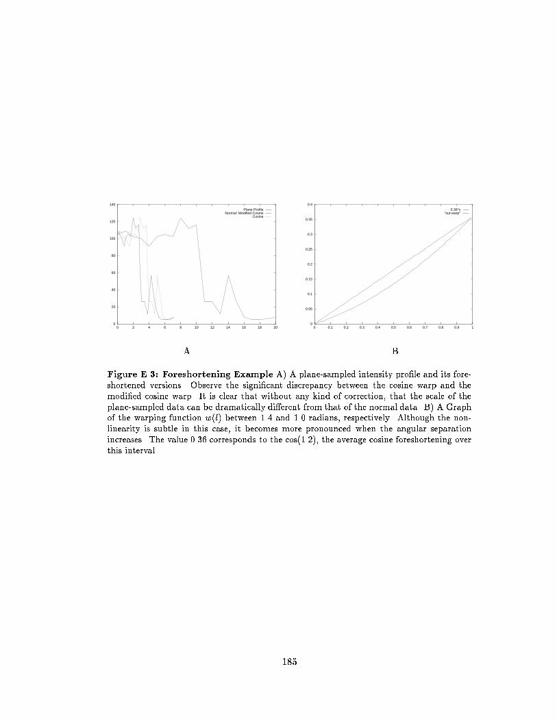
0

20

40

60

80

100

120

140

0 2 4 6 8 10 12 14 16 18 20

Plane ProfileNormal: Modified Cosine

Cosine

0

0.05

0.1

0.15

0.2

0.25

0.3

0.35

0.4

0 0.1 0.2 0.3 0.4 0.5 0.6 0.7 0.8 0.9 1

0.36*x"out-warp"

A B

Figure E�� Foreshortening Example A� A plane�sampled intensity pro�le and its fore�shortened versions� Observe the signi�cant discrepancy between the cosine warp and themodi�ed cosine warp� It is clear that without any kind of correction� that the scale of theplane�sampled data can be dramatically di�erent from that of the normal data� B� A Graphof the warping function w�l� between �� and �� radians� respectively� Although the non�linearity is subtle in this case� it becomes more pronounced when the angular separationincreases� The value �� corresponds to the cos�� the average cosine foreshortening overthis interval�

��

Appendix F

T� Boundary Model Database

The �� boundary models shown in Figure F�� were used in the boundary detection phase of

the segmentation scheme�

Model � Edge Number

M� ��

M� ��

M� ��

M� ��

M� ��

M� ��

M� ��

M� ��

M� ��

M��

M��

M��

Table F�� Model Parameters The value of � and the edge index are shown for eachmodel� The tolerance was the same for all models except the coarse models introduced tocope with boundary occlusion and foreshortening severe e�ects� A lower value was assignedto these models� since they were more likely to match undesirable features if not suitablyconstrained�

Each pro�le is shown to scale� and has an associated �tolerance� which corresponds to the

parameter � used in Chapter �� This value determines the set of absolute constraints imposed

on each model� If the value is low� the model can only exhibit low vertical variation! a high

value means the model can exhibit signi�cant vertical variation from instance to instance�

For very large values� the associated absolute constraints become super�uous� and the model

is only subject to relative segment constraints�

This will almost certainly result in erroneous boundary detection� particularly in regions

where the boundary is occluded� The values of �� as well as the edge number for each model�

are shown in Table F��

��

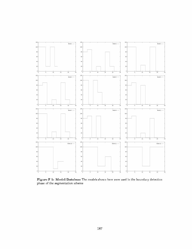
0

20

40

60

80

100

120

0 5 10 15 20 25

Model 1

0

20

40

60

80

100

120

0 5 10 15 20 25

Model 2

0

20

40

60

80

100

120

0 5 10 15 20 25

Model 3

0

20

40

60

80

100

120

0 5 10 15 20 25

Model 4

0

20

40

60

80

100

120

0 5 10 15 20 25

Model 5

0

20

40

60

80

100

120

0 5 10 15 20 25

Model 6

0

20

40

60

80

100

120

0 5 10 15 20 25

Model 7

0

20

40

60

80

100

120

0 5 10 15 20 25

Model 8

0

20

40

60

80

100

120

0 5 10 15 20 25

Model 9

0

20

40

60

80

100

120

0 5 10 15 20 25

Model 10

0

20

40

60

80

100

120

0 5 10 15 20 25

Model 11

0

20

40

60

80

100

120

0 5 10 15 20 25

Model 12

Figure F�� Model DatabaseThe models shown here were used in the boundary detectionphase of the segmentation scheme�

��

Bibliography

�� N� Andreasan et al� Techniques for measuring sulcal�gyral patters in the brain as visualized through magnetic resonance imaging� brainplot and brainmap� Proc Natl AcadSci� �� January ��

�� Y� BarShalom and T�E� Fortmann� Tracking and Data Association� Academic Press��

�� E� Bardinet� N� Ayache� and L� Cohen� Fitting of isosurfaces using superquadrics andfreeform deformations� In Proc of the IEEE workshop on biomedical image analysis��

�� R� Bartels� J� Beatty� and B� Barsky� An introduction to splines for use in computergraphics and geometric modelling� MorganKaufmann� San Mateo� California� ��

�� P� Besl and N� McKay� A method for registration of �d shapes� IEEE PAMI� ��February ��

�� R� M� Bilder et al� Absence of regional hemispheric volume asymmetries in �rstepisodeschizophrenia� American Journal of Psychiatry� �� Oct ��

�� C� Bishop� Neural Networks for Pattern Recognition� Oxford University Pres� ��

�� A� Blake� R� Curwen� and A� Zisserman� A framework for spatiotemporal control in thetracking of visual contours� Intl Journal of Comp Vis� ��

�� H� Blum� Biological shape and visual science part i�� J Theor Biol� ��

�� H� Blum and R� Nagel� Shape description using weighted symmetric axis features� Pat�tern Recognition� ��

�� F� Bookstein� Principal warps� thinplate splines and the decomposition of deformations�IEEE Transactions on Pattern Analysis and Machine Intelligence� pages �� May��

�� M� Brady and G� Scott� Parallel algorithms for shape representation� In I� Page� editor�Parallel architectures and computer vision� pages �� Oxford Science Publications��

�� C� Brechbuhler� G� Gerig� and O� Kubler� Parametrization of closed surfaces for �dshape description� Computer Vision and Image Understanding� �� March��

�� C� Brechb)uler� G� Gerig� and G� Sz+ekely� Compensation of spatial inhomogeneity inmri based on a parametric bias estimate� In Karl H� Hoehne and Ron Kikinis� editors�Proceedings of VBC�� volume �� of Lecture Notes in Computer Science� pages �� SpringerVerlag� ��

��

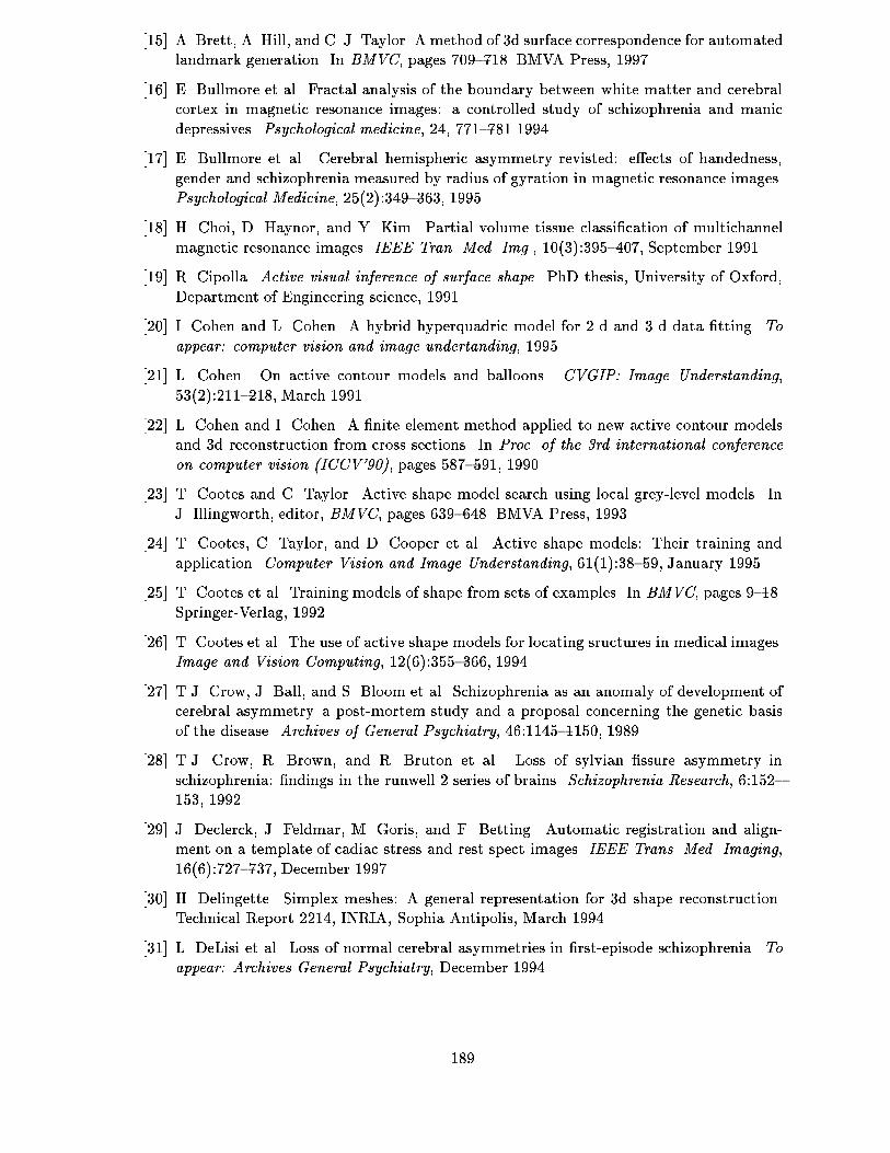
�� A� Brett� A� Hill� and C� J� Taylor� A method of �d surface correspondence for automatedlandmark generation� In BMVC� pages �� BMVA Press� ��

�� E� Bullmore et al� Fractal analysis of the boundary between white matter and cerebralcortex in magnetic resonance images� a controlled study of schizophrenia and manicdepressives� Psychological medicine� ��

�� E� Bullmore et al� Cerebral hemispheric asymmetry revisted� e�ects of handedness�gender and schizophrenia measured by radius of gyration in magnetic resonance images�Psychological Medicine� ��

�� H� Choi� D� Haynor� and Y� Kim� Partial volume tissue classi�cation of multichannelmagnetic resonance images� IEEE Tran Med Img� �� September ��

�� R� Cipolla� Active visual inference of surface shape� PhD thesis� University of Oxford�Department of Engineering science� ��

�� I� Cohen and L� Cohen� A hybrid hyperquadric model for �d and �d data �tting� Toappear� computer vision and image undertanding� ��

�� L� Cohen� On active contour models and balloons� CVGIP� Image Understanding�� March ��

�� L� Cohen and I� Cohen� A �nite element method applied to new active contour modelsand �d reconstruction from cross sections� In Proc of the �rd international conferenceon computer vision �ICCV�� pages ��

�� T� Cootes and C� Taylor� Active shape model search using local greylevel models� InJ� Illingworth� editor� BMVC� pages �� BMVA Press� ��

�� T� Cootes� C� Taylor� and D� Cooper et al� Active shape models� Their training andapplication� Computer Vision and Image Understanding� �� January ��

�� T� Cootes et al� Training models of shape from sets of examples� In BMVC� pages ��SpringerVerlag� ��

�� T� Cootes et al� The use of active shape models for locating sructures in medical images�Image and Vision Computing� ��

�� T�J� Crow� J� Ball� and S� Bloom et al� Schizophrenia as an anomaly of development ofcerebral asymmetry� a postmortem study and a proposal concerning the genetic basisof the disease� Archives of General Psychiatry� ��

�� T�J� Crow� R� Brown� and R� Bruton et al� Loss of sylvian �ssure asymmetry inschizophrenia� �ndings in the runwell � series of brains� Schizophrenia Research� ��

�� J� Declerck� J� Feldmar� M� Goris� and F� Betting� Automatic registration and alignment on a template of cadiac stress and rest spect images� IEEE Trans Med Imaging�� December ��

�� H� Delingette� Simplex meshes� A general representation for �d shape reconstruction�Technical Report �� INRIA� Sophia Antipolis� March ��

�� L� DeLisi et al� Loss of normal cerebral asymmetries in �rstepisode schizophrenia� Toappear� Archives General Psychiatry� December ��

��

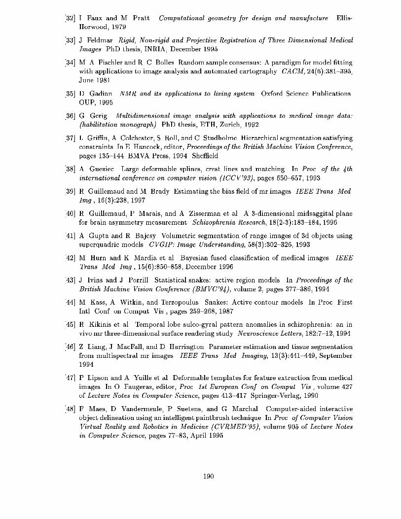
�� I� Faux and M� Pratt� Computational geometry for design and manufacture� EllisHorwood� ��

�� J� Feldmar� Rigid� Non�rigid and Projective Registration of Three Dimensional MedicalImages� PhD thesis� INRIA� December ��

�� M� A� Fischler and R� C� Bolles� Random sample consensus� A paradigm for model �ttingwith applications to image analysis and automated cartography� CACM� �� June ��

�� D� Gadian� NMR and its applications to living system� Oxford Science Publications�OUP� ��

�� G� Gerig� Multidimensional image analysis with applications to medical image data��habilitation monograph�� PhD thesis� ETH� Zurich� ��

�� L� Gri�n� A� Colchester� S� Roll� and C� Studholme� Hierarchical segmentation satisfyingconstraints� In E� Hancock� editor� Proceedings of the British Machine Vision Conference�pages �� BMVA Press� �� She�eld�

�� A� Gueziec� Large deformable splines� crest lines and matching� In Proc of the �thinternational conference on computer vision �ICCV�� pages ��

�� R� Guillemaud and M� Brady� Estimating the bias �eld of mr images� IEEE Trans MedImg� ��

�� R� Guillemaud� P� Marais� and A� Zisserman et al� A �dimensional midsaggital planefor brain asymmetry measurement� Schizophrenia Research� ��

�� A� Gupta and R� Bajcsy� Volumetric segmentation of range images of �d objects usingsuperquadric models� CVGIP� Image Understanding� ��

�� M� Hurn and K� Mardia et al� Bayesian fused classi�cation of medical images� IEEETrans Med Img� �� December ��

�� J� Ivins and J� Porrill� Statistical snakes� active region models� In Proceedings of theBritish Machine Vision Conference �BMVC�� volume �� pages ��

�� M� Kass� A� Witkin� and Terzopoulus� Snakes� Active contour models� In Proc� FirstIntl� Conf� on Comput� Vis�� pages ��

�� R� Kikinis et al� Temporal lobe sulcogyral pattern anomalies in schizophrenia� an invivo mr threedimensional surface rendering study� Neuroscience Letters� ��

�� Z� Liang� J� MacFall� and D� Harrington� Parameter estimation and tissue segmentationfrom multispectral mr images� IEEE Trans Med Imaging� �� September��

�� P� Lipson and A� Yuille et al� Deformable templates for feature extraction from medicalimages� In O� Faugeras� editor� Proc �st European Conf on Comput Vis� volume ��of Lecture Notes in Computer Science� pages �� SpringerVerlag� ��

�� F� Maes� D� Vandermeule� P� Suetens� and G� Marchal� Computeraided interactiveobject delineation using an intelligent paintbrush technique� In Proc of Computer VisionVirtual Reality and Robotics in Medicine �CVRMED�� volume �� of Lecture Notesin Computer Science� pages �� April ��

��

�� F� Maes et al� Automatic image partitioning for generic object segmentation in medicalimages� In Y� Bizais� C� Barillot� and R� Di Paola� editors� Computational Imaging andVision� volume �� pages �� Kluwer Academic Publishers� June ��

�� P� C� Marais� R� Guillemaud� and M� Sakuma et al� Visualising cerebral asymmetry�In Proc of Visualisation in Biomedical Computing� volume �� of Lecture Notes inComputer Science� �� pages �� SpringerVerlag� ��

�� T� McInerney and D� Terzopolous� Topologically adaptable snakes� In Proc of the �thinternational conference on computer vision �ICCV�� pages ��

�� J� Montagnat and H� Delingette� Volumetric medical images segmentation using shapeconstrained deformable models� In Proc of Computer Vision Virtual reality and Roboticsin Medicine �CVRMED�� March ��

�� C� Nastar and N� Ayache� Fast segmentation� tracking and analysis of deformable objects�In Proc of the �th international conference on computer vision �ICCV�� pages ��

�� A� Rinck� Magnetic resonance in medicine� Blackwell Scienti�c Publications� ��

�� S� R)oll and A� Colchester et� al� Intensitybased object extraction from �d medical imagesincluding a correction for partial volume errors� In BMVC� pages �� BMVA Press��

�� R� Ronfard� Regionbased strategies for active contour models� Intl J of comp vis��

�� L� E� Scales� Introduction to Non�Linear Optimization� Macmillan Computer ScienceSeries� Macmillan� ��

�� R� Sedgewick� Algorithms� Addison Wesley� ��

�� M� Shenton et al� Abnomalities of the left temporal lobe and thought disorder inschizophrenia� The new england journal of medicine� �� Aug ��

�� H� SoltanianZadeh� J� Windham� and A� Yagle� Optimal transformation for correctingpartial volume averaging e�ects in magentic resonance imaging� IEEE Tran Nucl Sci�� August ��

�� L� Staib and J� Duncan� Deformable fourier models for surface �nding in �d images� InR� Robb� editor� Proceedings of VBC�� pages ��

�� G� Sz+ekely� A� Kelemen� C� Brechb)uler� and G� Gerig� Segmentation of �d and �d objectsfrom mri volume data using constrained elastic deformations of �exible fourier contourand surface models� Medical Image Analysis� � ��

�� D� Terzopolous and A� Witkin� Symmetryseeking models for �d object reconstruction�In Proc of the �st international conference on computer vision �ICCV�� pages ��

�� D� Terzopoulos and D� Metaxas� Dynamic �D models with local and global deformations� deformable superquadrics� IEEE Transactions on Pattern Analysis and MachineIntelligence� ��

�� N� Thacker� A� Jackson� X� Zhu� and K� Li� Accuracy of tissue volume estimation in nmrimages� In Second British Conference on Medical Image Understanding and Analysis�pages �� Leeds� England� July ��

��

�� G�A� Thibodean and K�T� Patton� Anatomy and Physiology� Mosby� St Louis� �rdedition� ��

�� M� Vasilescu and D� Terzopoulos� Adapative meshes and shells� In Proc of Int Confon Computer Vision and Pattern Recognition �CVPR�� pages ��

�� K� Vincken� A� Koster� and M� Viergever� Probabilistic segmentation of partial volumevoxels� Pattern Recognition Letters� �� May ��

�� L� WeiChung� L� ChengChung� and C� Chintu� Dynamic elastic interpolation for �dmedical image reconstruction from serial cross sections� IEEE Trans Med Imaging�� September ��

�� W� Wells� W� Grimson� R� Kikinis� and F� Jolesz� Invivo intensity correction andsegmentation of magnetic resonance image data� AAAI Med Imaging� pages ��April ��

�� R� Whitaker� Algorithms for implicit deformable models� In Proc of �th internationalconference on computer vision �ICCV�� pages ��

�� D� L� Wilson� An Improved Planning Protocol for the Endovascular Treatment of In�tracranial Aneurysms� PhD thesis� University of Oxford� Department of EngineeringScience� ��

�� Z� Zhang� Iterative point matching for registration of freeform curves and surfaces�International Journal of Computer Vision� �� December ��

�� A� Zijdenbos and B� Dawarit et al� Automatic detection of intracranial contours in mriimages� Comput Med Imag and Graphics� ��

�� R� Zipursky et al� Widespread cerebral gray matter volume de�cits in schizophrenia�Archives General Psychiatry� �� March ��

��

The Segmentation of Sparse MR Images

Documents