The Secret Behind The Tortoise and the Hare - American ...

The Secret Behind The Tortoise and the Hare:Information Design in Contests∗

Job Market Paper

Alejandro Melo Ponce†

This version—November, 2018Click here for current version

Abstract

I analyze the optimal information disclosure problem under commitment of a “contest de-signer” in a class of binary action contests with incomplete information about the abilities of theplayers. If the contest designer wants to incentivize the players to play in equilibrium a particularstrategy profile, she can design an information disclosure rule, formally a stochastic communi-cation mechanism, to which she will commit and then use to “talk” with the players. The maintool to carry out the analysis is the concept of Bayes Correlated Equilibrium recently introducedin the literature. I find that the optimal information disclosure rules involves private informationrevelation (manipulation), which is also cost-effective for the designer. Furthermore, the optimaldisclosure rule involves asymmetric and in most cases correlated signals that convey only partialinformation about the abilities of the players.

JEL classification: C72, C79, D44, D82, D83.Keywords: information design, contests, implementation, incomplete information, Bayes CorrelatedEquilibrium.

1 Introduction

Have you ever wondered why the hare took a nap? Everybody knows well the fable.1 But how manyof us ever think about who organized such a curious contest. Imagine there was a fox behind it. Hedecided the where, when andwho of the competition. He could also speak with the contestants beforethe big hour. Maybe he told the tortoise not to give up, the hare is the fastest but weird things could

∗This paper was previously presented at various places with the title Information Design in Contests†Department of Economics, Stony Brook University. E-mail: [email protected]. I am pro-

foundly grateful to my advisor, Pradeep Dubey, for his continuous and invaluable help and encouragement with this project.I also wish to thank Ting Liu, Yair Tauman, Sandro Brusco, Vasiliki Skreta, Marcos Fernandes, Laura Karpuska, CamiloRubbini, Yijiao Liu, David Ruiz G., Michael Kramm, and seminar audiences at the 28th & 29th Stony Brook InternationalConferences on Game Theory, the 2017 Econometric Society Summer School, the 2018 Midwest Economic Association An-nual Meeting and the 2018 Econometric Society AustralasianMeeting for helpful comments and discussions. Special thanksto Brenda Cuellar Marines for her invaluable feedback and support. All remaining errors are my own.

1Aesop, “The Tortoise and the Hare”, fable 226 in the Perry Index.

1

happen. Talking to the hare, he may drop that it takes half a day for the tortoise to walk a similardistance. We all know the end of the story: the tortoise won and the fox made a fortune bettingagainst the hare. Let us take a look at how the fox did the magic.

The trick lies in the position of the fox. An agent with privileged information can use it in itsfavor. We have a lot of examples from daily life. A pollster could influence an election by sharingsome information with the parties running in the election. Imagine there are two candidates andcandidate A has a slight advantage over candidate B. The pollster can convince candidate B that inthe last poll there was a technical draw. So the campaign strategy must adapt if they want to getmore votes and be the winners. The pollster can share the information with candidate A or not. If thepollster shares, the candidate can adapt immediately so he can compete in the new scenario. But ifthe candidate does not get the information, adaption will take time and he could loose valuable votes.

Many examples abound where there is a third party who is in a position to alter the final resultsof a “competition” by modifying, in first instance, the behavior of the participants. The key is thetools that she posses and the way she uses them. For example, the third party could alter monetaryrewards. But instead, she can do the magic by manipulating the information that the players observe,without increasing her costs. Without further ado, let us turn to the matter in hand.

I present a model that illustrates how information manipulation can be used to alter the results ofa contest. The model is deliberately simple so as to derive its conclusions with minimal fuss while atthe same time providing a rich ground for its analysis.

Consider a principal who intends to organize a contest between two players. The principal, whichwe identify as she, henceforth will be referred to as “the contest designer”. In the contest there is aprize that is to be awarded to the player, each of which we identify as he, with the highest output.The output from each player is determined by his innate ability and the effort that he undertakes.Each player is presumed to always know his ability. The contest designer acts as a third-party tothe contest between the players in the sense that she does not participate in the strategic interactionbetween the players. We assume that the designer cannot manipulate the structure of the contest butcan only manipulate the information that the players observe by communicating it to them.

The contest, whose basic structure follows the one in Dubey (2013), belongs to a class of gameswith binary actions, namely to shirk or work, and with incomplete information about the abilitiesof the players, which are also assumed to be binary, either weak or strong. The class of contestsis parameterized by the value of a common prize, the cost of exerting effort, the private first-orderbeliefs that the players hold about their rival’s ability and the value to the designer, in terms of outputproduced, of the effort profile chosen by the players.

The designer wants to manipulate the beliefs of the players so that they play in equilibrium aparticular effort profile. In order to carry out this manipulation, the contest designer can design aninformation disclosure rule, which formally is a stochastic communication mechanism, to which shewill commit and then use to “talk” to the players. This structure endows the contest designer withmore commitment power in the sense that it will allow her to commit to send any distribution ofmessages that she desires as a function of the realized ability vector before learning it. This communi-

2

cation structure will become publicly known to the players. After this stage, the agents will observethe realized messages according to the information disclosure rule and will update their beliefs aboutthe ability of their rival, i.e. their first-order beliefs, their beliefs about the first-order beliefs of theirrival, i.e. their second-order beliefs, and so on.

The main tool to carry out the analysis and search for the optimal information disclosure rulefollows the general methodology introduced in Taneva (2015). The goal of the designer is to designan information disclosure rule for each contest which will induce an effort profile as a Bayes NashEquilibrium (BNE) with the property that such profile maximizes the designer’s objective in expec-tation. Under this view, the designer would have to first characterize the set of all BNE under allpossible information structures. The novelty here is that in contrast to Taneva (2015), we have anenvironment in which the players already possess private information about their abilities, so the setof information structures that we consider need to respect this restriction. Although performing thischaracterization program seems like an insurmountable task, we follow Taneva’s approach in whichwe appeal to the notion of Bayes Correlated Equilibrium, introduced by Bergemann andMorris (2016),which will allow us to characterize the set of all Bayes Nash Equilibria associated with each contestand with the prior private information of the players. Given the assumption that the players alreadyhave some prior private information about the ability of their rival, we need to use the full powerof Bergemann and Morris’s result2 It turns out that in our contest environment in which the playersare informed of their own ability, it comes at almost no cost extending the characterization of Tanevasince the players have distributed knowledge3 of the ability vector. Thus, when the designer learnsthe true ability vector before communicating with the players, she does not know anything more thatthe players already don’t know when they pool their information together.

We find that optimal information disclosure rules in contests involve private information revela-tion (manipulation). The optimal disclosure rule involves asymmetric and, in a robust set of parame-ters, correlated messages to each player. Themessages involved in the optimal information disclosurerule convey only partial information about the abilities of the players. The intuition behind this resultcan be most clearly understood in the two player contest environment that we describe in this paper.When both players have similar abilities, in an ex post assessment of the contest the players find thatthe competition is evenly poised and each player will find it worthwhile to put effort since they havean equal shot at obtaining the prize. On the other hand, when the players have disparate abilities, anex post assessment of the contest would lead the players to shirk with high probability, particularlyfor the strong player. Thus if it were possible, it would be in the interest of the designer to fullyand publicly inform the players when they are similar and tell them nothing when they are different.However, no information disclosure rule can implement the previous state of affairs, since giving fulland public information when the players are similar immediately makes it common knowledge not

2Theorem 1 in Bergemann and Morris (2016) which provides an epistemic relationship between the set of Bayes Cor-related Equilibria under some initial information structure and the set of Bayes Nash Equilibria under all informationstructures that expand the first one.

3The two players, by pooling their knowledge together, can deduce the full ability vector. See Fagin, Halpern, Moses,and Vardi (2004, p. 23). Bergemann and Morris (2013) call this property distributed certainty in a language that is morestandard in the game theory literature.

3

only this fact but also the corresponding event when the players hear nothing when they are differ-ent. Therefore, it will be in the interest of the designer to only partially reveal information in such away that the true ability vector never becomes common knowledge. This is one of the reasons thatmakes private information necessary. It turns out that it is the beliefs of the weak player that drivethe incentive to put effort in the contest, since it is his actions and beliefs when competing against astrong player that actually motivate the strong to work. Hence, the optimal revelation scheme altersnot only the first-order beliefs of the players but also the higher-order hierarchies in a non-trivial way.Precisely for the previous reasons, public revelation of information is not optimal, since it generatessymmetric hierarchies of beliefs even when the players are different in their abilities. In particular,for a robust set of parameters, the optimal information scheme follows the rule of informing the under-dog: at some messages, the weak player will become more informed, with respect to his prior privateinformation, about the ability vector; whereas at other messages, the weak player will become fullyinformed of the ability vector; however, neither these two facts will be common knowledge betweenthe two players.

The explicit characterization of the optimal information disclosure rule for every contest allowsus to perform an important comparative statics analysis. Suppose that the prize the designer awardsconsists of a fraction of the total output produced by the contestants. In this scenario, the designercan engage in information design while at the same time altering the value of the prize. While the“revenue” side of information design is intuitively well understood, we are know attaching a “cost” toactually carrying out the information manipulation. We find necessary and sufficient conditions onthe parameters of the game to ensure that a private, asymmetric and partial information revelationscheme is optimal for the designer and I also provide conditions for when it is the case that givingno information is optimal. The main message is that we find that under a robust set of parametersfor which manipulating information while giving a relatively small prize is doubly optimal: it doesnot only provide incentives for the players to work but it also does it in the most cost-efficient waypossible.

The rest of the section is devoted to a survey of the related literature.

1.1 Literature Review

This paper belongs to a very recent and active literature on information design. This strand of theliterature about communication in games is different from the cheap talk literature as establishedby Crawford and Sobel (1982) because the assumption that the information designer can crediblycommit to an information transmission strategy before learning the true state of the world. Theone-agent version of the problem has been extensively studied in the literature since the seminalcontribution of Kamenica and Gentzkow (2011) on Bayesian Persuasion, which is preceded by theworks of Aumann, Maschler, and Stearns (1995), Brocas and Carrillo (2007) and Benoît and Dubra(2011). Kamenica andGentzkow provide a characterization of the optimal information design problemfor the case of a single sender and receiver using techniques from convex analysis. Their elegantresults allows for a clear characterization of optimality of an information structure in the single-

4

agent case. Since then, the one agent-version has been the subject of a productive effort by manyauthors in many different areas and applications (e.g. Gentzkow and Kamenica (2014); Ely, Frankel,and Kamenica (2015); Kolotilin, Mylovanov, Zapechelnyuk, and Li (2017); Lipnowski and Mathevet(2018), to name a few).

On the other hand, the theory of information design in games is still at an early stage. Never-theless, optimal solutions have been derived in specific environments, for example as in Vives (1988);Morris and Shin (2002) and Angeletos and Pavan (2007). The most closely related papers to this onein terms of techniques are Taneva (2015) and Bergemann and Morris (2016), as both provide the sys-tematic approach, based on a revelation-principle style methodology, to approach information designproblems. As mentioned before, the method is based on the notion of Bayes Correlated Equilibriumthat characterizes all Bayes Nash Equilibrium outcomes under all possible information structures. Wetake advantage of this formulation to simplify and fully characterize the information design problemin contests discussed in this paper. Another closely related paper is Mathevet, Perego, and Taneva(2016) in which they push forward the theory to provide a characterization of the solution to the in-formation design problem in terms of belief-hierarchy distribution instead of information structures.This allows them to provide an expression of the optimal solution in games in terms of an optimalprivate and public component, where the later part comes from concavification, effectively extend-ing Kamenica and Gentzkow’s characterization. Their results assume no prior private informationfrom the players. In particular, they discuss some qualitative properties of belief-hierarchy distri-butions and information structures which we adapt for our problem of a contest with prior privateinformation from the players.

For a recent an in-depth survey of the literature on information design, the reader is encouragedto consult Bergemann and Morris (2018) and Kamenica (2018).

The literature on asymmetric information and information disclosure in contests motivates thispaper. These issues have been the focus of recent work (Fey, 2008; Lim and Matros, 2009; Münster,2009; Morath and Münster, 2013; Epstein and Mealem, 2013; Gürtler, Münster, and Nieken, 2013;Fu, Gürtler, and Münster, 2013; Dubey, 2013; Denter, Morgan, and Sisak, 2014; Fu, Lu, and Zhang,2016; Einy, Moreno, and Shitovitz, 2017). Some of these papers study issues related to how an agentshould disclose information about his private attributes. Other papers in which a designer is present,study how a designer should disclose “performance evaluations” or study disclosure policies in a one-sided asymmetric information environment. In particular, Lim and Matros (2009) and Fu et al. (2013,2016) consider the problem of how to reveal information about contestants entries when these arestochastic. Denter et al. (2014) analyze the incentives of a privately informed contestant to disclose hisinformation to his opponent and the incentives for transparency of the designer. Dubey (2013), fromwhich we take the basic environment, analyzes the impact of null versus complete information in acontest in terms of expected output from the players. These last strand of articles focus on comparingthe cases of no disclosure versus full disclosure. In this paper, we extend the discussion towards ana-lyzing partial information disclosure rules and contribute towards a classification of their qualitativerichness and their impact in manipulating the behavior of the players. We also find that focusing

5

only on no disclosure versus full disclosure is with loss of generality, since the optimal informationdisclosure rules require in general partial revelation of information.

A closely related paper is Zhang and Zhou (2016), in which they analyze the Bayesian persuasionproblem in a Tullock contest with one-sided asymmetric information. They assume that one contes-tant has imperfect information about the cost function of his opponent while the other one is perfectlyinformed. The contest designer decides how to disclose this information to the imperfectly informedcontestant using general disclosure rules with can span the whole spectrum between null disclosureto full disclosure. However, in their analysis, they focus on public disclosure rules, which buys thema great deal of technical convenience, since they can apply the insights from Kamenica and Gentzkowto find an optimal solution in their problem. Compared to Zhang and Zhou, our paper extends theanalysis of optimal information disclosure in contests in two directions: we assume all contestantsto have incomplete information about while holding private information about the a payoff relevantparameter of the contest, and we allow for fully general information disclosure rules, since the dis-tinction between public and private information and full versus partial disclosure becomes crucial incontests.

Finally, another very closed related paper is Kramm (2018), who focuses on a multi-task Tullockcontest in which there is incomplete information from all players about how the success in the contestwill depend on the effortmixture put on different tasks. Krammalso considers amethodology inspiredby Bergemann and Morris (2016) to solve for the optimal information policy. A feature in Kramm’scontest environment is that the players do not hold any prior private information. Nevertheless hederives similar results to ours: he also finds that there is an important distinction between privateand public information and that in order for the information disclosure policy to benefit the designer,private information provides the right informational advantage for the players to behave in the waythat the designer intends. In his environment, he finds that optimal information disclosure involvessometimes disclosing information to a weak player in a particular task while in other scenarios it isoptimal to inform only contestants who are strong in a particular task. Compare this to our resultsthat say that in general both players should be partially informed while in some cases the weak playerbecomes fully informed. However, the nature of the information disclosure rule in this paper is suchthat the event that a player becomes fully informed does not become common knowledge when ithappens. Also the information disclosure policy sometimes leaves first-order beliefs untouched whileoperating on the second and higher-order hierarchy.

The rest of the paper follows the following structure. In section 2 we present the description of themodel: the contest designer and the players; the role of the designer in manipulating information; andthe extended game that is induced by the designer’s choice of information disclosure rule. Section 3describes the role of the Bayes Correlated Equilibrium notion in simplifying the optimal informationdisclosure problem in the contest. Section 4 presents the characterization of the equilibrium behaviorfor two particular information disclosure rules; these results will be ancillary to establishing andcomparing the main results of the paper. Section 5 presents the main results of the paper, namely thefull characterization of the optimal information disclosure rules for the family of contest that we are

6

considering and the cost-benefit analysis of designing information in the contest. Section 6 concludesand describes some extensions and avenues for future research.

2 Model

A principal, which wewill refer from now on as the contest designer, intends to run a contest betweentwo players. The contest designer acts as an external agent to the contest between the players andher only role is to disclose information to the players but other than that she does not participatein the strategic interaction. In particular, we assume that the contest designer can only manipulateinformation, but not the structure of the contest.

The contest between the two players follows the structure of the basic model in Dubey (2013),from which we take the particular specification of the contest.

The two players are assumed to be risk neutral and ex-ante symmetric. Each player i 2 f1; 2g

can have one of two abilities, ai 2 f˛; ˇg D Ai � R, where ˛ < ˇ. Thus, we identify ˛ with aweak player and ˇ with a strong player. Each player can choose from two effort levels ei 2 f0; 1g D

fShirk;Workg D Ei . As usual, a 2 A D A1 � A2 will denote the ability vector and e 2 E D E1 � E2

the effort vector.Each player i , given his ability and effort chosen, produces output according to the production

function f W Ei � Ai ! R given by

f .ei ; ai / D

˚ai if ei D 0

k.ai /ai if ei D 1

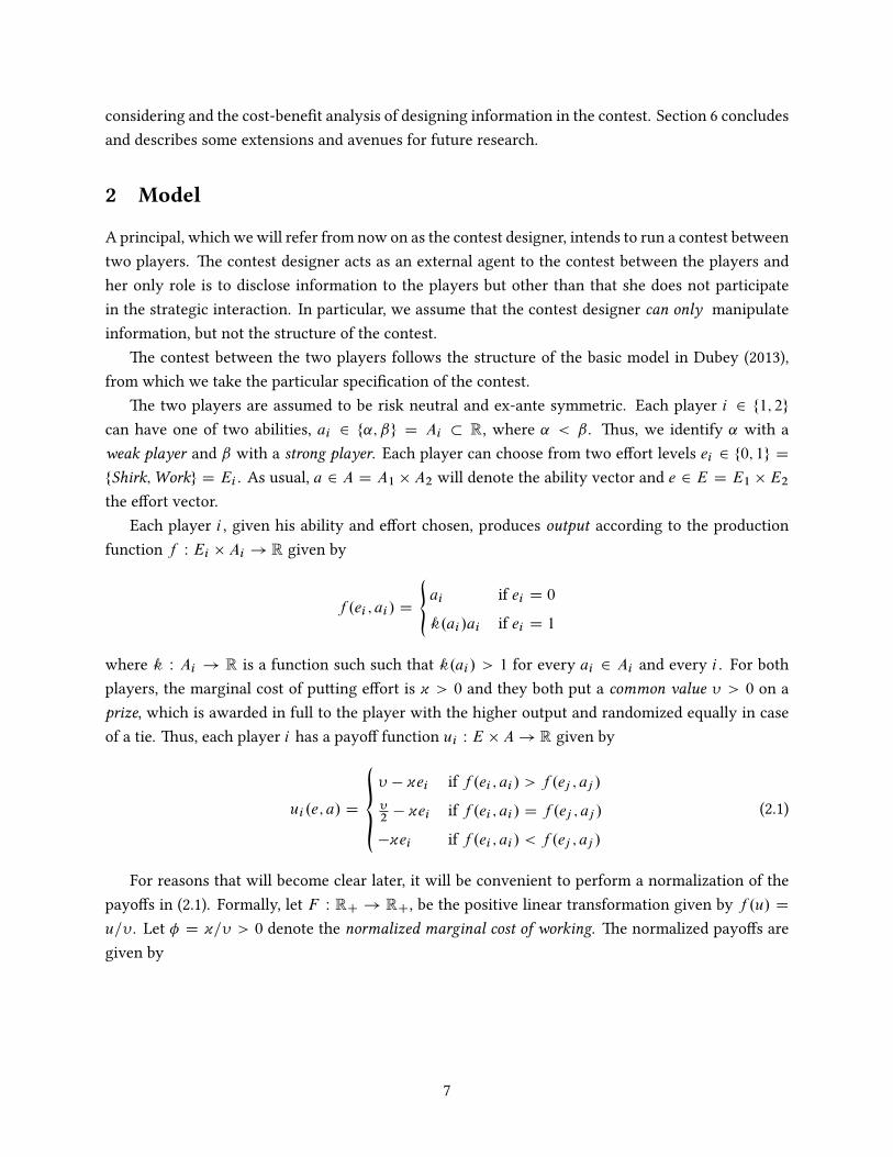
where k W Ai ! R is a function such such that k.ai / > 1 for every ai 2 Ai and every i . For bothplayers, the marginal cost of putting effort is ~ > 0 and they both put a common value � > 0 on aprize, which is awarded in full to the player with the higher output and randomized equally in caseof a tie. Thus, each player i has a payoff function ui W E � A ! R given by

ui .e; a/ D

„� � ~ei if f .ei ; ai / > f .ej ; aj /�2

� ~ei if f .ei ; ai / D f .ej ; aj /

�~ei if f .ei ; ai / < f .ej ; aj /

(2.1)

For reasons that will become clear later, it will be convenient to perform a normalization of thepayoffs in (2.1). Formally, let F W RC ! RC, be the positive linear transformation given by f .u/ D

u=� . Let � D ~=� > 0 denote the normalized marginal cost of working. The normalized payoffs aregiven by

7

Oui .e; a/ D f .ui .e; a// D

„1 � �ei if f .ei ; ai / > f .ej ; aj /;12

� �ei if f .ei ; ai / D f .ej ; aj /;

��ei if f .ei ; ai / < f .ej ; aj /:

(2.2)

We will impose some assumptions on the parameters of the model to make the analysis tractableand comparable with the results in Dubey (2013).

A1. (Minimum valuation). � < 1, or equivalently ~ < �:This assumption precludes that the contestdoes not become trivial by making shirking strictly dominant under any information structure.This assumption enables us to focus on the failure to work caused by strategic competition.Notice that when � < 1=2 or equivalently 2~ < � , the prize is large enough to guarantee evenif it is split equally in the case of a tie, the players still find it worthwile to put effort.

A2. (Monotonicity of Output). k.ai /ai is strictly monotonic for each ai 2 Ai and every i .

A3. (Ordering of Output). ˇ < k.˛/˛. This assumption is concerned with the ordering of k.˛/˛

and ˇ, i.e. the output when the weak player works and the one from the strong player when heshirks respectively. Intuitively, this assumption says that if a weak player works, then he canbeat a strong player who shirks.

Let K � R4CC denote the set of productivities that satisfy assumptions A.2 and A.3,

K D˚.˛; ˇ;k.˛/˛;k.ˇ/ˇ/ 2 R4CCj˛ < ˇ < k.˛/˛ < k.ˇ/ˇ

:

An arbitrary 4-tuple from this set will be denoted by k.We will assume that the players are privately and independently informed of their own ability and

that their beliefs4 about their rival’s ability after being informed is constant across abilities, strictlypositive and symmetric between players. These restrictions imply the existence of a symmetric, sta-tistically independent common prior from which the posterior beliefs are derived. We can collect theprevious observations into the following assumption.

A4. (Common prior & Constant beliefs). For each player i D 1; 2, the posterior beliefs about thevector of abilities a 2 A are symmetric between players and constant across abilities, i.e.

prob.˛j˛/ D prob.˛jˇ/ D 2 .0; 1/:

These beliefs are induced by a common prior P that satisfies statistical independence, as fol-lows:

P .˛; ˛/ D 2; P .˛; ˇ/ D P .ˇ; ˛/ D .1 � /; P .ˇ; ˇ/ D .1 � /2;

therefore5 P 2 int��.A/

�. Abusing notation, we will identify P with .

4Formally, these are the first order beliefs of the players about the state a 2 A5For any set X , �.X/ denotes the set of probability measures.

8

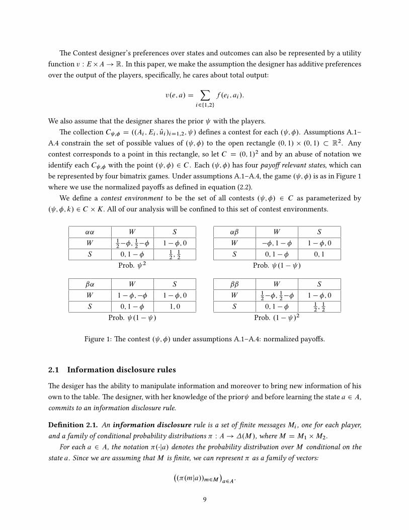
The Contest designer’s preferences over states and outcomes can also be represented by a utilityfunction v W E�A ! R. In this paper, we make the assumption the designer has additive preferencesover the output of the players, specifically, he cares about total output:

v.e; a/ DXi2f1;2g

f .ei ; ai /:

We also assume that the designer shares the prior with the players.The collection C ;� D ..Ai ; Ei ; Oui /iD1;2; / defines a contest for each . ; �/. Assumptions A.1–

A.4 constrain the set of possible values of . ; �/ to the open rectangle .0; 1/ � .0; 1/ � R2. Anycontest corresponds to a point in this rectangle, so let C D .0; 1/2 and by an abuse of notation weidentify each C ;� with the point . ; �/ 2 C . Each . ; �/ has four payoff relevant states, which canbe represented by four bimatrix games. Under assumptions A.1–A.4, the game . ; �/ is as in Figure 1where we use the normalized payoffs as defined in equation (2.2).

We define a contest environment to be the set of all contests . ; �/ 2 C as parameterized by. ; �; k/ 2 C �K: All of our analysis will be confined to this set of contest environments.

˛˛ W S

W 12

��; 12

�� 1 � �; 0

S 0; 1 � � 12; 12

Prob. 2

˛ˇ W S

W ��; 1 � � 1 � �; 0

S 0; 1 � � 0; 1

Prob. .1 � /

ˇ˛ W S

W 1 � �;�� 1 � �; 0

S 0; 1 � � 1; 0

Prob. .1 � /

ˇˇ W S

W 12

��; 12

�� 1 � �; 0

S 0; 1 � � 12; 12

Prob. .1 � /2

Figure 1: The contest . ; �/ under assumptions A.1–A.4: normalized payoffs.

2.1 Information disclosure rules

The desiger has the ability to manipulate information and moreover to bring new information of hisown to the table. The designer, with her knowledge of the prior and before learning the state a 2 A,commits to an information disclosure rule.

Definition 2.1. An information disclosure rule is a set of finite messages Mi , one for each player,and a family of conditional probability distributions � W A ! �.M/, whereM D M1 �M2.

For each a 2 A, the notation �.�ja/ denotes the probability distribution over M conditional on thestate a. Since we are assuming thatM is finite, we can represent � as a family of vectors:�

.�.mja//m2M

�a2A

:

9

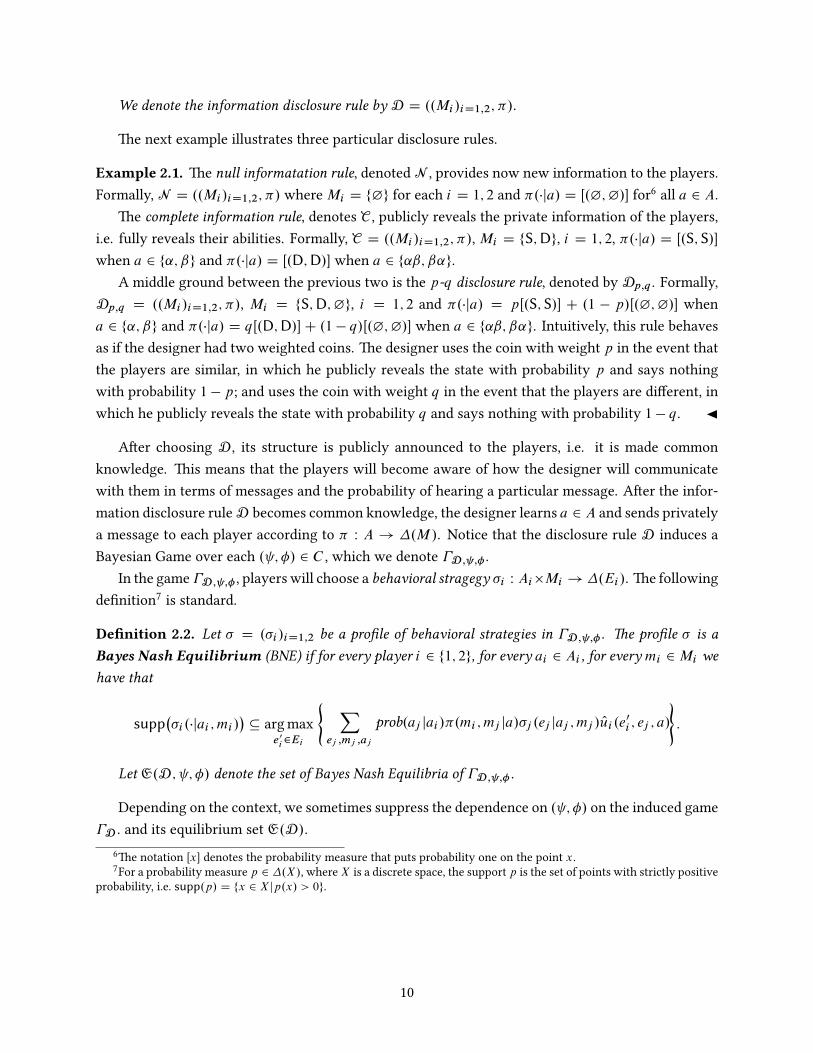
We denote the information disclosure rule by D D ..Mi /iD1;2; �/.

The next example illustrates three particular disclosure rules.

Example 2.1. The null informatation rule, denoted N , provides now new information to the players.Formally, N D ..Mi /iD1;2; �/ whereMi D f¿g for each i D 1; 2 and �.�ja/ D Œ.¿;¿/� for6 all a 2 A.

The complete information rule, denotes C , publicly reveals the private information of the players,i.e. fully reveals their abilities. Formally, C D ..Mi /iD1;2; �/,Mi D fS;Dg, i D 1; 2, �.�ja/ D Œ.S;S/�when a 2 f˛; ˇg and �.�ja/ D Œ.D;D/� when a 2 f˛ˇ; ˇ˛g.

A middle ground between the previous two is the p-q disclosure rule, denoted by Dp;q . Formally,Dp;q D ..Mi /iD1;2; �/, Mi D fS;D;¿g, i D 1; 2 and �.�ja/ D pŒ.S;S/� C .1 � p/Œ.¿;¿/� whena 2 f˛; ˇg and �.�ja/ D qŒ.D;D/�C .1 � q/Œ.¿;¿/� when a 2 f˛ˇ; ˇ˛g. Intuitively, this rule behavesas if the designer had two weighted coins. The designer uses the coin with weight p in the event thatthe players are similar, in which he publicly reveals the state with probability p and says nothingwith probability 1 � p; and uses the coin with weight q in the event that the players are different, inwhich he publicly reveals the state with probability q and says nothing with probability 1 � q: J

After choosing D , its structure is publicly announced to the players, i.e. it is made commonknowledge. This means that the players will become aware of how the designer will communicatewith them in terms of messages and the probability of hearing a particular message. After the infor-mation disclosure rule D becomes common knowledge, the designer learns a 2 A and sends privatelya message to each player according to � W A ! �.M/. Notice that the disclosure rule D induces aBayesian Game over each . ; �/ 2 C , which we denote �D; ;� .

In the game �D; ;� , players will choose a behavioral stragegy �i W Ai�Mi ! �.Ei /. The followingdefinition7 is standard.

Definition 2.2. Let � D .�i /iD1;2 be a profile of behavioral strategies in �D; ;� . The profile � is aBayes Nash Equilibrium (BNE) if for every player i 2 f1; 2g, for every ai 2 Ai , for every mi 2 Mi wehave that

supp��i .�jai ; mi /

�� argmax

e0i2Ei

( Xej ;mj ;aj

prob.aj jai /�.mi ; mj ja/�j .ej jaj ; mj / Oui .e0i ; ej ; a/

):

Let E.D ; ; �/ denote the set of Bayes Nash Equilibria of �D; ;� :

Depending on the context, we sometimes suppress the dependence on . ; �/ on the induced game�D : and its equilibrium set E.D/:

6The notation Œx� denotes the probability measure that puts probability one on the point x.7For a probability measure p 2 �.X/, whereX is a discrete space, the support p is the set of points with strictly positive

probability, i.e. supp.p/ D fx 2 X jp.x/ > 0g.

10

2.2 The contest design (information) problem

The expected payoff for the designer of information disclosure rule D and any strategy profile � fromthe players is

V.D ; � I ; �; k/ DXa;e

P.a/

0@Xm2M

�.mja/YiD1;2

�i .ei jai ; mi /

1A v.e; a/: (2.3)

The information design problem for the contest designer is given by

xV . ; �; k/ D maxD

max�2E. ;�;D/

V.D ; � I ; �; k/: (2.4)

Notice that in problem (2.4) we are assuming a selection criteria for equilibria8 which is the one thatbenefits the designer, in case there is multiplicity of equilibria in �D; ;� .

If we can find an optimal information disclosure rule D� that solves problem (2.4), it is not guar-anteed that such a rule will induce a unique equilibrium in the extended game. The only thing thatwe can guarantee is that in the game induced by D� there will be an equilibrium �� that will achievethe best effort profile for the designer. However, it may be the case that the optimal informationdisclosure rule also induces other equilibria different from ��. Thus, an important question is whatequilibrium effort profiles such equilibria engender and how these compare to the ones generated bythe profile ��. In order to answer this question we will need to characterize the whole equilibriumset E.D�; ; �/ of the extended game generated by the optimal information disclosure rule.

The next subsection introduces adequate notation and some definitions that will help us to char-acterize the equilibrium set.

2.3 The game and beliefs induced by an information disclosure rule

2.3.1 The induced game and the extended type space

Recall that, as described in subsection 2.1, once the information disclosure rule is chosen by the de-signer, he commits to it, in the sense that its probabilistic structure is disclosed publicly to the players,i.e. it is made common knowledge. Afterwards, the information disclosure rule is used to create themessages than then will be communicated privately and truthfully to the players.

The previous discussion implies that we can think about the prior information that the playersalready posses, i.e. knowledge of their own abilities, together with the message that they hear fromthe designer as their type in the incomplete information game �D . Formally the type space of eachplayer is Ti D Ai �Mi for i D 1; 2, where each type ti 2 Ti denotes the vector .ai ; mi /, i.e. player i ’sai is her ability type and mi is its message type.

Given the information disclosure rule D D ..Mi /iD1;2; �/, the probability that the type vector8As we will see below, for some special information disclosure rules and some values of the parameters � and , the

set E.D ; ; �/ is a singleton.

11

t D .t1; t2/ D�.a1; m1/; .a2; m2/

�2 T is realized, denoted by PT .t/, can be computed by9

PT .t/ D P.a/�.mja/: (2.5)

Of course, we will have that10 margA PT D P, i.e. the marginal with respect to the ability typesA of the joint measure PT must equal the original prior over A.

After player i learns his ability type aiand hears from the designer his message type mi , i.e. thetype ti D .ai ; mi /, he uses this information to form a posterior belief Opi W Ti ! �.Tj /

11 over thetypes of his rival tj 2 Tj that he deems possible:

Opi .tj jti / D prob.tj jti / D

�P�ai ;aj

���.mi ;mj /

ˇ.ai ;aj /

�P

ai ;mjP�ai ;a

0j

���.mi ;m

0j/ˇ.ai ;a

0j/� if ti 2 supp.margTi

PT /

0 otherwise.(2.6)

After an information disclosure rule D is put in place, the analysis of the extended game �D canbe carried out in the standard way by extending the type space to T , with PT being the common priorover it and each player i will calculate their respective posterior about the realized type vector t afterreceiving their own type ti .

However, there are situations in which we can further simplify the analysis by considering asmaller type space than T . Notice from equations (2.5) and (2.6), we could possibly have that allplayers assign probability 1 to some particular subsets of T or believe that types in another subsetare no longer possible after they receive their information. These ideas can be expressed rigorouslywith the help of the conditional probabilities as calculated by equation (2.6) by defining the notion ofa belief closed subsets of the type space.12

Definition 2.3. A subsetW D W1�W2 of T is called belief closed if for every player i D 1; 2,Wi � Ti

and for every ti 2 Wi , the posterior probability prob.�jti / assigns probability one to the set Wj , j ¤ i .

Thus, if the profile of players types t D .t1; t2/ is in the belief closed subset W , under a commonprior, this fact can be made common knowledge among the two players.

Consider now the equilibrium set E.D/ and let � W T ! �.E1/ � �.E2/ be a strategy profilebelonging to the equilibrium set. Then, let ��.�jt / 2 �.E/ be the induced product measure over E

9Rigorously, if we define hA W A �M ! A as hA.a;m/ D a and hM W A �M ! M as h.a;m/ D m, if t D .a;m/ thenPT .t/ D P

�hA.a;m/

���hM .a;m/jhA.a;m/

�.

10For a joint probability measure p 2 �.X � Y /, margX p 2 �.X/ denotes the marginal distribution over X induced byp.

11We depart form the usual notational convention in the literature that denotes the posterior belief of player i at his typeti about the rival’s type tj as Opi .ti /Œtj � and instead write this belief as Opi .tj jti /.

12The definition (Myerson, 1991, p. 81) of belief closed subsets is usually written in terms of the Universal BeliefSpace (Mertens and Zamir, 1985; Brandenburger and Dekel, 1993). However, the finite and consistent (common prior)type-space that we are using in this paper, a Harsanyi Model, can be embedded into the Universal Belief Space. Anothername in the literature for belief closed subsets is belief subspaces (Zamir, 2009). Whichever the definition or name thatwe use, the notion that they describe is similar: a subset that contains all the states for the world which are relevant tothe situation we are analyzing. Thus, a belief-closed subset describes events that become effectively common knowledgebetween the players when they happen.

12

for each t 2 supp .PT /, i.e. ��.ejt/ D �1.e1jt1/�2.e2jt2/ for each e 2 E and t 2 supp.PT /. Thetype action measure induced by the profile � will be denoted by �� 2 �.T � E/ and is given by�� .t; e/ D PT .t/��.ejt/ for each t 2 supp.PT / and each e 2 E . Notice that the expectation of theutility of the designer in equation (2.3) is taken with respect to �� . In particular, the expression inthe inner parenthesis of (2.3) is a posterior probability:

margA�E Œ�� �.a; e/

margAŒ�� �.a/for each a 2 A and each e 2 E;

and then each of these posteriors is averaged over .e; a/ 2 E � A using as weights the original priorprobability P.a/.

2.3.2 Hierarchies of beliefs and properties of information disclosure rules

Consider the extended Bayesian game �D induced by the information disclosure rule D and theextended type space associated with it, T D A � M . We have described previously in the previoussubsection how to calculate the posterior beliefs for the players about the type of their opponentfor each type they may end up having: their private information about their respective abilities andthe messages received from the designer. However, recall that the only payoff-relevant informationfrom the point of view of the players is their ability types, i.e. the vector a 2 A. So it is importantto understand how the information disclosure rule affect the beliefs of each player about a, i.e. theirfirst-order beliefs. Moreover, given the uncertainty the players have about the full vector of abilities a,and since the decisions the other player takes are relevant, then so are their beliefs about what beliefsabout a the opponent holds, i.e. their second-order beliefs. Similarly, since the second-order beliefs arerelevant and unknown to the players, then they must also hold beliefs about the second-order beliefs,i.e. their third-order beliefs and so on. Thus, the notion of the infinite hierarchies of beliefs pops upnaturally in our context.

Although Harsanyi’s (Harsanyi, 1967, 1968a,b) notion of type allows us to bypass explicitly con-sidering the infinite hierarchies of beliefs it is nevertheless instructive, for the purposes of this paper,to analyze how an information disclosure rule D impacts those hierarchies. In particular, the ex-plicit construction of the hierarchy of beliefs induced by an optimal information disclosure rule willallows us to describe what is its role in inducing the players to behave as intended by the designer.Furthermore, we will attempt to classify the optimal information disclosure rules by how they affectthe hierarchy of beliefs. Finally, this classification will depend on some properties of the informationdisclosure rules that depend on how they affect some or all levels of the hierarchy.

Because of the previous discussion we now present a discussion of how to extract the hierarchiesof beliefs from the extended type-space T and the posterior probabilities Opi W Ti ! �.Tj / from eachplayer. The construction that we present is standard (Battigalli, 2018; Maschler, Solan, and Zamir,2013), which we adapt to the current model in the paper.

13

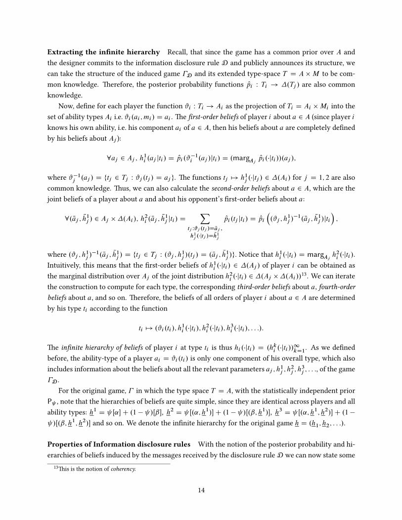
Extracting the infinite hierarchy Recall, that since the game has a common prior over A andthe designer commits to the information disclosure rule D and publicly announces its structure, wecan take the structure of the induced game �D and its extended type-space T D A �M to be com-mon knowledge. Therefore, the posterior probability functions Opi W Ti ! �.Tj / are also commonknowledge.

Now, define for each player the function #i W Ti ! Ai as the projection of Ti D Ai �Mi into theset of ability types Ai i.e. #i .ai ; mi / D ai . The first-order beliefs of player i about a 2 A (since player iknows his own ability, i.e. his component ai of a 2 A, then his beliefs about a are completely definedby his beliefs about Aj ):

8aj 2 Aj ; h1i .aj jti / D Opi .#

�1i .aj /jti / D .margAj

Opi .�jti //.aj /;

where #�1j .aj / D ftj 2 Tj W #j .tj / D aj g. The functions tj 7! h1j .�jtj / 2 �.Ai / for j D 1; 2 are also

common knowledge. Thus, we can also calculate the second-order beliefs about a 2 A, which are thejoint beliefs of a player about a and about his opponent’s first-order beliefs about a:

8. Naj ; Nh1j / 2 Aj ��.Ai /; h2i . Naj ;

Nh1j jti / DX

tj W#j .tj /D Naj ;

h1j.�jtj /D Nh1

j

Opi .tj jti / D Opi

�.#j ; h

1j /

�1. Naj ; Nh1j /jti

�;

where .#j ; h1j /�1. Naj ; Nh1j / D ftj 2 Tj W .#j ; h1j /.tj / D . Naj ; Nh1j /g: Notice that h1i .�jti / D margAj

h2i .�jti /.Intuitively, this means that the first-order beliefs of h1i .�jti / 2 �.Aj / of player i can be obtained asthe marginal distribution over Aj of the joint distribution h2i .�jti / 2 �.Aj ��.Ai //

13. We can iteratethe construction to compute for each type, the corresponding third-order beliefs about a, fourth-orderbeliefs about a, and so on. Therefore, the beliefs of all orders of player i about a 2 A are determinedby his type ti according to the function

ti 7! .#i .ti /; h1i .�jti /; h

2i .�jti /; h

3i .�jti /; : : :/:

The infinite hierarchy of beliefs of player i at type ti is thus hi .�jti / D .hki .�jti //1kD1

. As we definedbefore, the ability-type of a player ai D #i .ti / is only one component of his overall type, which alsoincludes information about the beliefs about all the relevant parameters aj ; h1j ; h2j ; h3j ; : : :, of the game�D .

For the original game, � in which the type space T D A, with the statistically independent priorP , note that the hierarchies of beliefs are quite simple, since they are identical across players and allability types: h1 D Œ˛�C .1� /Œˇ�, h2 D Œ.˛; h1/�C .1� /Œ.ˇ; h1/�, h3 D Œ.˛; h1; h2/�C .1�

/Œ.ˇ; h1; h2/� and so on. We denote the infinite hierarchy for the original game h D .h1; h2; : : :/.

Properties of Information disclosure rules With the notion of the posterior probability and hi-erarchies of beliefs induced by the messages received by the disclosure rule D we can now state some

13This is the notion of coherency.

14

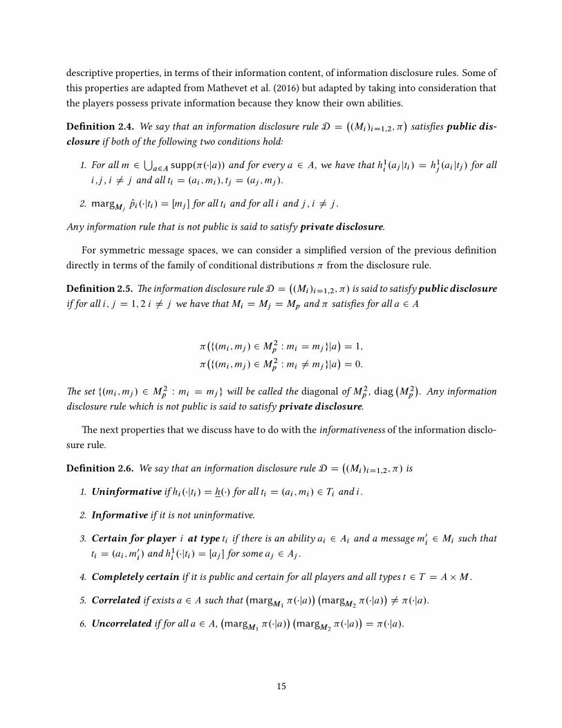
descriptive properties, in terms of their information content, of information disclosure rules. Some ofthis properties are adapted from Mathevet et al. (2016) but adapted by taking into consideration thatthe players possess private information because they know their own abilities.

Definition 2.4. We say that an information disclosure rule D D�.Mi /iD1;2; �

�satisfies public dis-

closure if both of the following two conditions hold:

1. For all m 2Sa2A supp.�.�ja// and for every a 2 A, we have that h1i .aj jti / D h1j .ai jtj / for all

i ,j , i ¤ j and all ti D .ai ; mi /; tj D .aj ; mj /.

2. margMjOpi .�jti / D Œmj � for all ti and for all i and j , i ¤ j .

Any information rule that is not public is said to satisfy private disclosure.

For symmetric message spaces, we can consider a simplified version of the previous definitiondirectly in terms of the family of conditional distributions � from the disclosure rule.

Definition 2.5. The information disclosure ruleD D�.Mi /iD1;2; �/ is said to satisfy public disclosure

if for all i; j D 1; 2 i ¤ j we have thatMi D Mj D Mp and � satisfies for all a 2 A

��f.mi ; mj / 2 M 2

p W mi D mj gja�

D 1;

��f.mi ; mj / 2 M 2

p W mi ¤ mj gja�

D 0:

The set f.mi ; mj / 2 M 2p W mi D mj g will be called the diagonal of M 2

p , diag�M 2p

�. Any information

disclosure rule which is not public is said to satisfy private disclosure.

The next properties that we discuss have to do with the informativeness of the information disclo-sure rule.

Definition 2.6. We say that an information disclosure rule D D�.Mi /iD1;2; �/ is

1. Uninformative if hi .�jti / D h.�/ for all ti D .ai ; mi / 2 Ti and i .

2. Informative if it is not uninformative.

3. Certain for player i at type ti if there is an ability ai 2 Ai and a message m0i 2 Mi such that

ti D .ai ; m0i / and h

1i .�jti / D Œaj � for some aj 2 Aj .

4. Completely certain if it is public and certain for all players and all types t 2 T D A �M .

5. Correlated if exists a 2 A such that�margM1

�.�ja/� �margM2

�.�ja/�

¤ �.�ja/.

6. Uncorrelated if for all a 2 A,�margM1

�.�ja/� �margM2

�.�ja/�

D �.�ja/.

15

Intuitively, an uninformative information disclosure rule leaves the players with the same beliefsas they had before receiving the message from the designer, while an informative rules alters theinfinite hierarchy of beliefs non-trivially. Under a certain information disclosure rule, some playerwith some ability type might come to belief with certainty that the true ability vector after hearing aparticular message from the designer. However, this may not hold true for other players or messages.Finally, if a rule is certain for all players and at all messages while at the same time being public, thenit is completely certain. This means that not only all players come to believe with certainty the trueability vector, but this fact also becomes common knowledge.

3 Simplifying the designer’s problem

The goal of this section is to describe the approach that we will take to obtain the solution of prob-lem (2.4). In the definition of this problem, notice that the space from which we take the “outside”maximization is the space of all finite-message information disclosure rules. This set is an infinitedimensional space. Consider two natural numbers n1 and n2 and let N D n1n2. Consider the mes-sage space M D M1 � M2 in which the individual message spaces contain respectively n1 and n2messages, so that theM contains N possible joint messages. Then for each a 2 A, the �.�ja/ 2 �.M/

is a point in the .N � 1/-dimensional simplex, i.e.

�.�ja/ 2 �N�1 D

˚x 2 RN W

NXjD1

xj D 1; xj � 0

Thus, the space of all finite-message information structures is given by

I D[

.n1;n2/2N2

n1n2DN

fM W M D M1 �M2; jM1j D n1; jM2j D n2g ���N�1

�4:

Therefore, as it is right now, finding the optimal disclosure rule in problem (2.4) is potentially veryhard, since the set I of decision variables is infinite-dimensional.

However, we can use a generalization of Aumann’s correlated equilibrium (Aumann, 1987, 1974)to games of incomplete information due to Bergemann and Morris (2016) to simplify the problem.

Definition 3.1. Let � W A ! �.E/ be a decision rule, i.e. a family of conditional probability distri-butions over E indexed by the states a 2 A. Then we say that � is a Bayes Correlated Equilibrium(BCE) of . ; �/inC if for each i D 1; 2, a 2 A and ei 2 Ei we have that

Xej ;aj

prob.aj jai /�.ei ; ej ja/ Oui .ei ; ej ; a/ �Xej ;aj

prob.aj jai /�.ei ; ej ja/ Oui .e0i ; ej ; a/ 8e0

i 2 Ei (3.1)

As we mentioned in the introduction, Taneva (2015) was the first one to to use the notion of a BCEto provide the general finte approach to derive the optimal information structure of the designer. Her

16

approach, which is the onewe follow in this paper, is based on the following theorem fromBergemannand Morris (2016), which provides the cornerstone of the analysis.

Theorem 3.2. (Bergemann and Morris, 2016, Thm. 1, p. 495). Decision rule � is a BCE of . ; �/ 2 C ifand only if there exists and information disclosure rule D and a BNE of �D; ;� which induces �. Strategyprofile b of �D induces � as follows:

�.eja/ DXm2M

�.mja/

0@ YiD1;2

bi .ei jai ; mi /

1A 8.a; e/ 2 A �E: (3.2)

If � is a BCE of ; � 2 C then the payoff for the designer from � is, when the productivities arek 2 K

V.�I ; �; k/ DXa;e

P.a/�.eja/v.e; a/: (3.3)

Therefore, what the theorem claims is that

xV . ; �; k/ D maxD

max�2E. ;�;D/

V.D ; � I ; �; k/ D max�2BCE. ;�/

V.�I ; �; k/: (3.4)

The inner maximization in the middle part of equation (3.4) implies that we are using an equi-librium selection criterion. In the theorem, the quantifier “there exists” is equivalent to this innermaximization. Thus, by using theorem 3.2 we cannot escape from the selection criterion. Changingthe quantifier in the statement of the theorem to for all implies changing the inner maximization fora minimization. With this qualification, then the information design problem becomes of finding thebest information rule assuming that the agents will play the worst equilibrium. In this case we can nolonger apply theorem 3.2. Recent contributions (Mathevet et al., 2016; Carroll, 2016) are attempts topush the analysis for this case, which the literature calls adversarial information design (Bergemannand Morris, 2018). However, we will show that in the model we are considering, the best equilibriumselection issue is diminished since in the equilibrium set induced by the optimal disclosure rule, thebest equilibrium turns out to be the unique pure strategy symmetric equilibrium generically.

After finding an optimal Bayes Correlated Equilibrium, it is straightforward to come up with anoptimal information structure. The next proposition, which is a corollary of theorem 3.2, explainshow to do it.

Proposition 3.3. Let ��. ; �; k/ 2 argmax�2BCE. ;�/ V.�I ; �; k/. An optimal information structureD� D .M �; ��/ can be constructed as follows:

• We set M � D M �1 � M �

2 where M �i D Ei for each i D 1; 2: The previous message space is

canonical in the sense that it will provide an action recommendation. Alternatively, any spaceM 0

which isomorphic toM � also works, i.e. if we can establish a bijectionM �i $ M 0

i for the individualmessage spaces for each i D 1; 2.

• We set ��.mja/ D ��.eja/ for all e 2 E , m 2 M � and a 2 A. In here M � stands for either thecanonical message space or any alternate message space that is isomorphnic to it.

17

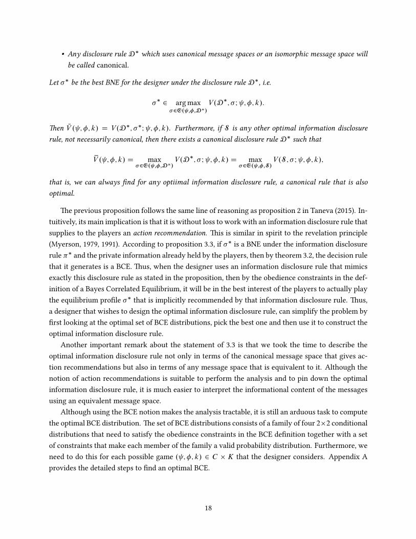
• Any disclosure rule D� which uses canonical message spaces or an isomorphic message space willbe called canonical.

Let �� be the best BNE for the designer under the disclosure rule D�, i.e.

��2 argmax�2E. ;�;D�/

V.D�; � I ; �; k/:

Then NV . ; �; k/ D V.D�; ��I ; �; k/. Furthermore, if S is any other optimal information disclosurerule, not necessarily canonical, then there exists a canonical disclosure rule D� such that

xV . ; �; k/ D max�2E. ;�;D�/

V.D�; � I ; �; k/ D max�2E. ;�;S/

V.S ; � I ; �; k/;

that is, we can always find for any optiimal information disclosure rule, a canonical rule that is alsooptimal.

The previous proposition follows the same line of reasoning as proposition 2 in Taneva (2015). In-tuitively, its main implication is that it is without loss to work with an information disclosure rule thatsupplies to the players an action recommendation. This is similar in spirit to the revelation principle(Myerson, 1979, 1991). According to proposition 3.3, if �� is a BNE under the information disclosurerule �� and the private information already held by the players, then by theorem 3.2, the decision rulethat it generates is a BCE. Thus, when the designer uses an information disclosure rule that mimicsexactly this disclosure rule as stated in the proposition, then by the obedience constraints in the def-inition of a Bayes Correlated Equilibrium, it will be in the best interest of the players to actually playthe equilibrium profile �� that is implicitly recommended by that information disclosure rule. Thus,a designer that wishes to design the optimal information disclosure rule, can simplify the problem byfirst looking at the optimal set of BCE distributions, pick the best one and then use it to construct theoptimal information disclosure rule.

Another important remark about the statement of 3.3 is that we took the time to describe theoptimal information disclosure rule not only in terms of the canonical message space that gives ac-tion recommendations but also in terms of any message space that is equivalent to it. Although thenotion of action recommendations is suitable to perform the analysis and to pin down the optimalinformation disclosure rule, it is much easier to interpret the informational content of the messagesusing an equivalent message space.

Although using the BCE notion makes the analysis tractable, it is still an arduous task to computethe optimal BCE distribution. The set of BCE distributions consists of a family of four 2�2 conditionaldistributions that need to satisfy the obedience constraints in the BCE definition together with a setof constraints that make each member of the family a valid probability distribution. Furthermore, weneed to do this for each possible game . ; �; k/ 2 C � K that the designer considers. Appendix Aprovides the detailed steps to find an optimal BCE.

18

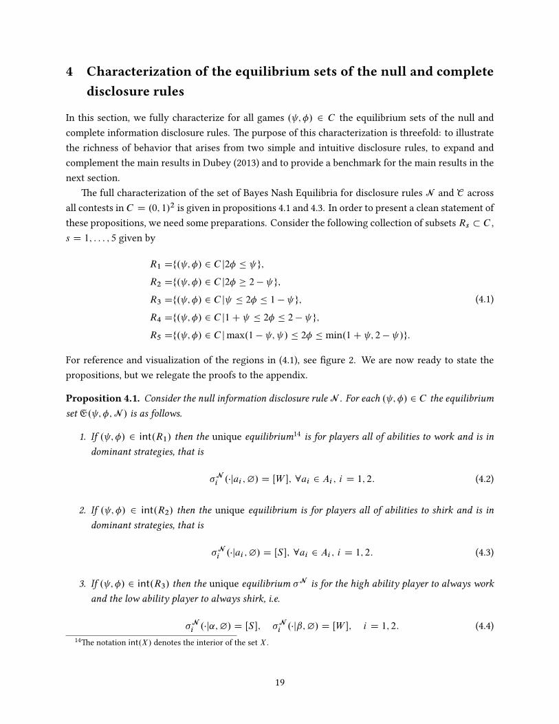
4 Characterization of the equilibrium sets of the null and completedisclosure rules

In this section, we fully characterize for all games . ; �/ 2 C the equilibrium sets of the null andcomplete information disclosure rules. The purpose of this characterization is threefold: to illustratethe richness of behavior that arises from two simple and intuitive disclosure rules, to expand andcomplement the main results in Dubey (2013) and to provide a benchmark for the main results in thenext section.

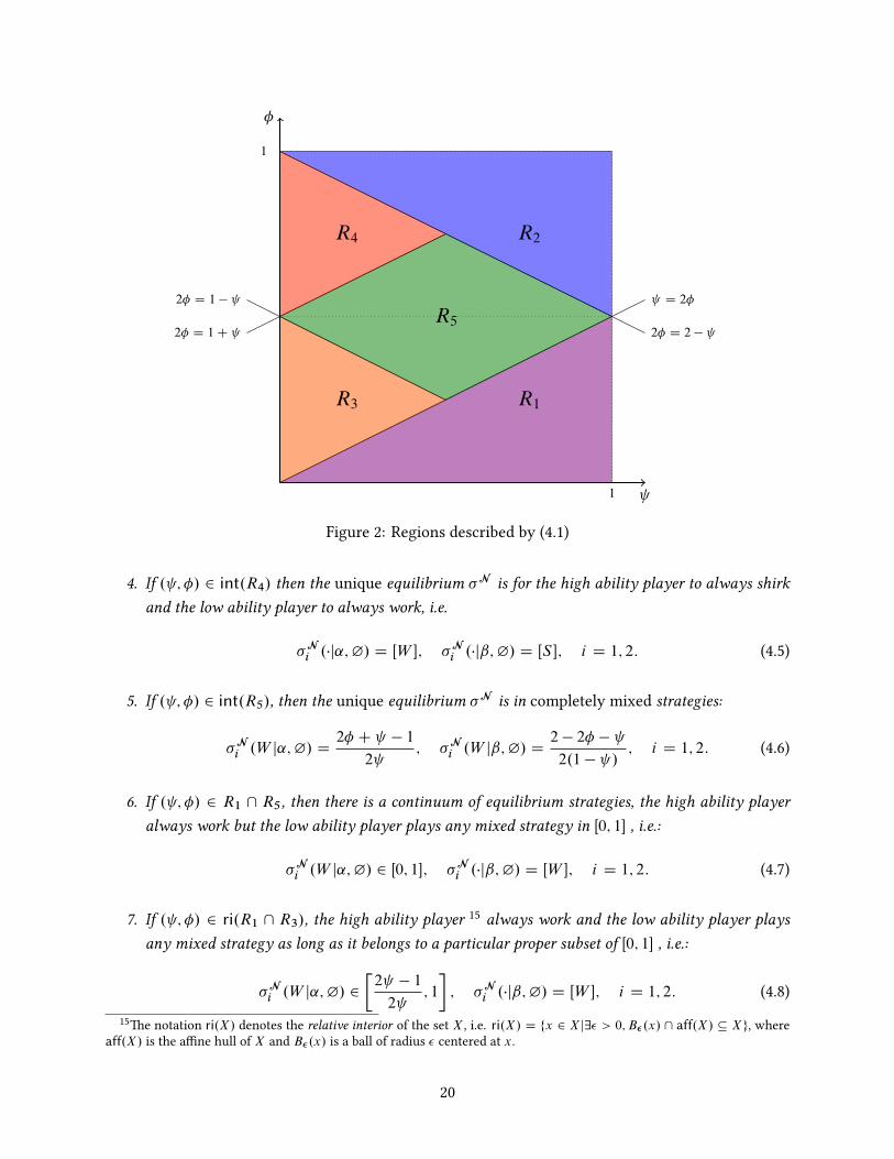
The full characterization of the set of Bayes Nash Equilibria for disclosure rules N and C acrossall contests in C D .0; 1/2 is given in propositions 4.1 and 4.3. In order to present a clean statement ofthese propositions, we need some preparations. Consider the following collection of subsets Rs � C ,s D 1; : : : ; 5 given by

R1 Df. ; �/ 2 C j2� � g;

R2 Df. ; �/ 2 C j2� � 2 � g;

R3 Df. ; �/ 2 C j � 2� � 1 � g;

R4 Df. ; �/ 2 C j1C � 2� � 2 � g;

R5 Df. ; �/ 2 C jmax.1 � ; / � 2� � min.1C ; 2 � /g:

(4.1)

For reference and visualization of the regions in (4.1), see figure 2. We are now ready to state thepropositions, but we relegate the proofs to the appendix.

Proposition 4.1. Consider the null information disclosure rule N . For each . ; �/ 2 C the equilibriumset E. ; �;N / is as follows.

1. If . ; �/ 2 int.R1/ then the unique equilibrium14 is for players all of abilities to work and is indominant strategies, that is

�Ni .�jai ;¿/ D ŒW �; 8ai 2 Ai ; i D 1; 2: (4.2)

2. If . ; �/ 2 int.R2/ then the unique equilibrium is for players all of abilities to shirk and is indominant strategies, that is

�Ni .�jai ;¿/ D ŒS�; 8ai 2 Ai ; i D 1; 2: (4.3)

3. If . ; �/ 2 int.R3/ then the unique equilibrium �N is for the high ability player to always workand the low ability player to always shirk, i.e.

�Ni .�j˛;¿/ D ŒS�; �N

i .�jˇ;¿/ D ŒW �; i D 1; 2: (4.4)14The notation int.X/ denotes the interior of the set X .

19

�

1

1

D 2�2� D 1 �

2� D 1C 2� D 2 �

R1

R2

R3

R4

R5

Figure 2: Regions described by (4.1)

4. If . ; �/ 2 int.R4/ then the unique equilibrium �N is for the high ability player to always shirkand the low ability player to always work, i.e.

�Ni .�j˛;¿/ D ŒW �; �N

i .�jˇ;¿/ D ŒS�; i D 1; 2: (4.5)

5. If . ; �/ 2 int.R5/, then the unique equilibrium �N is in completely mixed strategies:

�Ni .W j˛;¿/ D

2� C � 1

2 ; �N

i .W jˇ;¿/ D2 � 2� �

2.1 � /; i D 1; 2: (4.6)

6. If . ; �/ 2 R1 \ R5, then there is a continuum of equilibrium strategies, the high ability playeralways work but the low ability player plays any mixed strategy in Œ0; 1� , i.e.:

�Ni .W j˛;¿/ 2 Œ0; 1�; �N

i .�jˇ;¿/ D ŒW �; i D 1; 2: (4.7)

7. If . ; �/ 2 ri.R1 \ R3/, the high ability player 15 always work and the low ability player playsany mixed strategy as long as it belongs to a particular proper subset of Œ0; 1� , i.e.:

�Ni .W j˛;¿/ 2

�2 � 1

2 ; 1

�; �N

i .�jˇ;¿/ D ŒW �; i D 1; 2: (4.8)15The notation ri.X/ denotes the relative interior of the set X , i.e. ri.X/ D fx 2 X j9� > 0;B�.x/ \ aff.X/ � Xg, where

aff.X/ is the affine hull of X and B�.x/ is a ball of radius � centered at x.

20

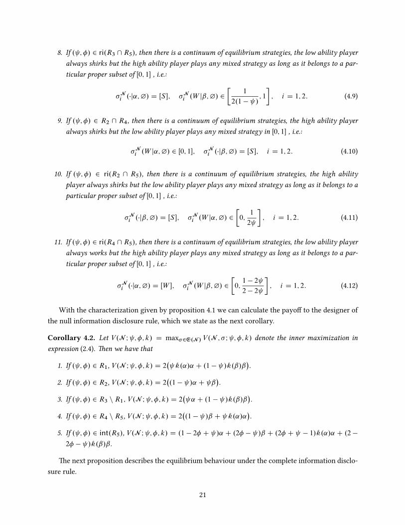
8. If . ; �/ 2 ri.R3 \R5/, then there is a continuum of equilibrium strategies, the low ability playeralways shirks but the high ability player plays any mixed strategy as long as it belongs to a par-ticular proper subset of Œ0; 1� , i.e.:

�Ni .�j˛;¿/ D ŒS�; �N

i .W jˇ;¿/ 2

�1

2.1 � /; 1

�; i D 1; 2: (4.9)

9. If . ; �/ 2 R2 \ R4, then there is a continuum of equilibrium strategies, the high ability playeralways shirks but the low ability player plays any mixed strategy in Œ0; 1� , i.e.:

�Ni .W j˛;¿/ 2 Œ0; 1�; �N

i .�jˇ;¿/ D ŒS�; i D 1; 2: (4.10)

10. If . ; �/ 2 ri.R2 \ R5/, then there is a continuum of equilibrium strategies, the high abilityplayer always shirks but the low ability player plays any mixed strategy as long as it belongs to aparticular proper subset of Œ0; 1� , i.e.:

�Ni .�jˇ;¿/ D ŒS�; �N

i .W j˛;¿/ 2

�0;

1

2

�; i D 1; 2: (4.11)

11. If . ; �/ 2 ri.R4 \R5/, then there is a continuum of equilibrium strategies, the low ability playeralways works but the high ability player plays any mixed strategy as long as it belongs to a par-ticular proper subset of Œ0; 1� , i.e.:

�Ni .�j˛;¿/ D ŒW �; �N

i .W jˇ;¿/ 2

�0;1 � 2

2 � 2

�; i D 1; 2: (4.12)

With the characterization given by proposition 4.1 we can calculate the payoff to the designer ofthe null information disclosure rule, which we state as the next corollary.

Corollary 4.2. Let V.N I ; �; k/ D max�2E.N / V.N ; � I ; �; k/ denote the inner maximization inexpression (2.4). Then we have that

1. If . ; �/ 2 R1, V.N I ; �; k/ D 2� k.˛/˛ C .1 � /k.ˇ/ˇ

�:

2. If . ; �/ 2 R2, V.N I ; �; k/ D 2�.1 � /˛ C ˇ

�:

3. If . ; �/ 2 R3 nR1; V .N I ; �; k/ D 2� ˛ C .1 � /k.ˇ/ˇ

�:

4. If . ; �/ 2 R4 nR5, V.N I ; �; k/ D 2�.1 � /ˇ C k.˛/˛

�:

5. If . ; �/ 2 int.R5/, V.N I ; �; k/ D .1 � 2� C /˛ C .2� � /ˇ C .2� C � 1/k.˛/˛ C .2 �

2� � /k.ˇ/ˇ:

The next proposition describes the equilibrium behaviour under the complete information disclo-sure rule.

21

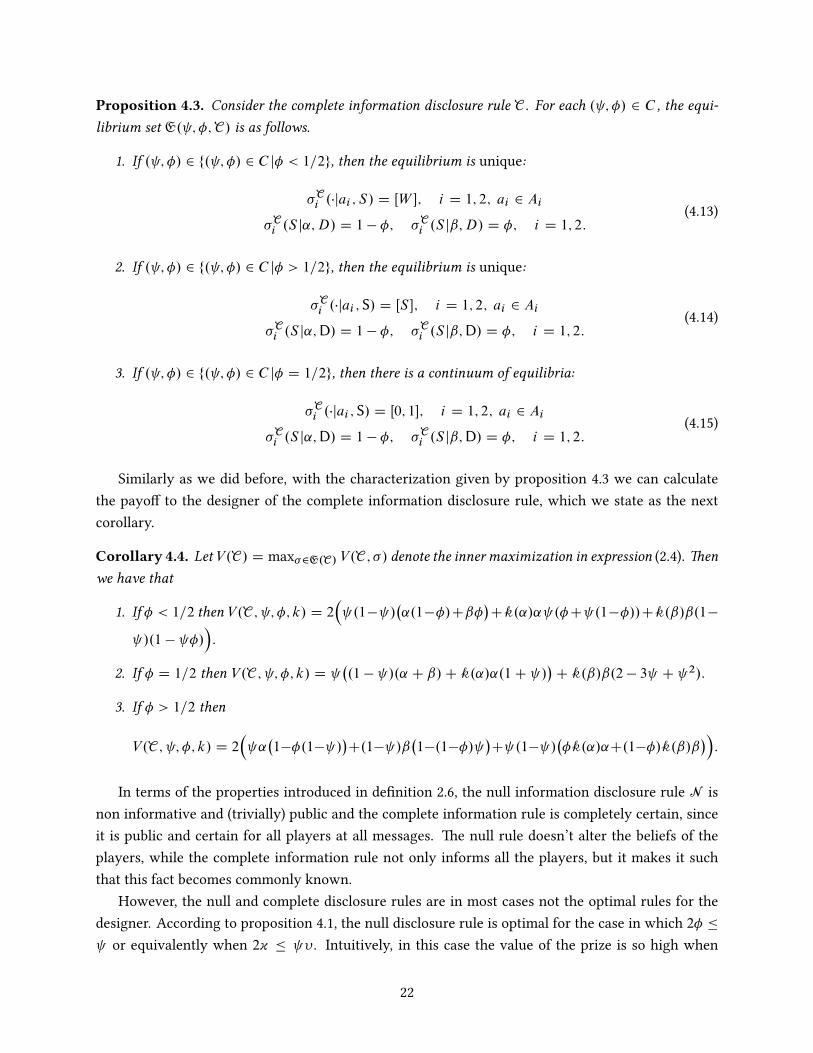
Proposition 4.3. Consider the complete information disclosure rule C . For each . ; �/ 2 C , the equi-librium set E. ; �;C/ is as follows.

1. If . ; �/ 2 f. ; �/ 2 C j� < 1=2g, then the equilibrium is unique:

�Ci .�jai ; S/ D ŒW �; i D 1; 2; ai 2 Ai

�Ci .S j˛;D/ D 1 � �; �C

i .S jˇ;D/ D �; i D 1; 2:(4.13)

2. If . ; �/ 2 f. ; �/ 2 C j� > 1=2g, then the equilibrium is unique:

�Ci .�jai ;S/ D ŒS�; i D 1; 2; ai 2 Ai

�Ci .S j˛;D/ D 1 � �; �C

i .S jˇ;D/ D �; i D 1; 2:(4.14)

3. If . ; �/ 2 f. ; �/ 2 C j� D 1=2g, then there is a continuum of equilibria:

�Ci .�jai ;S/ D Œ0; 1�; i D 1; 2; ai 2 Ai

�Ci .S j˛;D/ D 1 � �; �C

i .S jˇ;D/ D �; i D 1; 2:(4.15)

Similarly as we did before, with the characterization given by proposition 4.3 we can calculatethe payoff to the designer of the complete information disclosure rule, which we state as the nextcorollary.

Corollary 4.4. Let V.C/ D max�2E.C/ V.C ; �/ denote the inner maximization in expression (2.4). Thenwe have that

1. If � < 1=2 then V.C ; ; �; k/ D 2� .1� /

�˛.1��/Cˇ�

�Ck.˛/˛ .�C .1��//Ck.ˇ/ˇ.1�

/.1 � �/�:

2. If � D 1=2 then V.C ; ; �; k/ D �.1 � /.˛ C ˇ/C k.˛/˛.1C /

�C k.ˇ/ˇ.2 � 3 C 2/:

3. If � > 1=2 then

V.C ; ; �; k/ D 2� ˛

�1��.1� /

�C.1� /ˇ

�1�.1��/

�C .1� /

��k.˛/˛C.1��/k.ˇ/ˇ

��:

In terms of the properties introduced in definition 2.6, the null information disclosure rule N isnon informative and (trivially) public and the complete information rule is completely certain, sinceit is public and certain for all players at all messages. The null rule doesn’t alter the beliefs of theplayers, while the complete information rule not only informs all the players, but it makes it suchthat this fact becomes commonly known.

However, the null and complete disclosure rules are in most cases not the optimal rules for thedesigner. According to proposition 4.1, the null disclosure rule is optimal for the case in which 2� �

or equivalently when 2~ � � . Intuitively, in this case the value of the prize is so high when

22

compared to the cost of putting effort that both players find strictly dominant to put effort withoutthe need to receive more information from the part of the designer. On the other hand, the resultsin Dubey (2013) find that the complete information rule C performs, in general, better than the nullrule N when 2� > and � < 1=2, or equivalently, 2~ > � and 2~ < �: Propositions 4.1 and 4.3extend the results in Dubey (2013) by extending the parameter space to all � 2 .0; 1/. Thefore, a trivialcalculation shows that the complete information disclosure rule, in general, also performs better thanthe null rule when 1=2 � � < 1 or equivalently when � � 2~. However, the analysis the null andcomplete information rules is not sufficient to pin down the optimum for the contest informationdesign problem. It is possible to construct a rule that outperforms the complete information rule C

for all cases in which the null information rule N is not optimal. In the next section, we show howto construct the globally optimal information disclosure rule for the information design problem.

5 Optimal information Disclosure: Main results

In this section we discuss the main results of the paper. The first subsection describes the full char-acterization of the optimal information disclosure rule for each contest in C � K. After presentingthese set of results, we illustrate them by means of a numerical example that is meant to showcasethe main features of the characterization. Finally in the last subsection, by fully taking advantage ofour characterization, we perform a comparative statics exercise in which we allow the designer toalter the value of the prize simultaneously while engaging in information design. The results of thisexercise deliver the necessary and sufficient conditions at which the optimal information structurenot only achieves the goals of the designer but it also does at the cheapest possible way. All proofsare relegated to appendix A.

5.1 Characterization of the optimal information disclosure rule

We begin by describing the main features of the optimal information disclosure rule. In order todescribe it in a succinct way, we need to introduce some new terminology and notation that will beuseful.

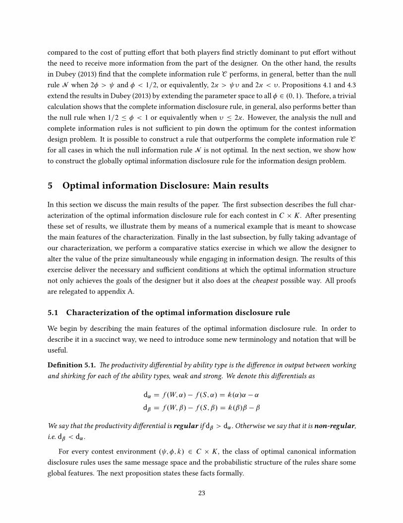
Definition 5.1. The productivity differential by ability type is the difference in output between workingand shirking for each of the ability types, weak and strong. We denote this differentials as

d˛ D f .W; ˛/ � f .S; ˛/ D k.˛/˛ � ˛

dˇ D f .W; ˇ/ � f .S; ˇ/ D k.ˇ/ˇ � ˇ

We say that the productivity differential is regular if dˇ > d˛: Otherwise we say that it is non-regular,i.e. dˇ < d˛:

For every contest environment . ; �; k/ 2 C � K, the class of optimal canonical informationdisclosure rules uses the same message space and the probabilistic structure of the rules share someglobal features. The next proposition states these facts formally.

23

Proposition 5.2 (Optimal Information Disclosure Rules). The class of optimal canonical informationdisclosure rules

D D

„

D W�.Mi /iD1;2; �

�W

there exists . ; �; k/ 2 C �K such that

.1/ xV . ; �; k/ D max�2E. ;�;D/

V.D ; � I ; �; k/;

.2/D is equivalent to a canonical rule.

…

has symmetric message spaces given by

Mi D fHard-Fought;:Hard-Foughtg D fmH ;:mH g for i D 1; 2,

and � W A ! �.M/ is given by

�.�j˛˛/ mH :mH

mH �˛ 0

:mH 0 1 � �˛

�.�j˛ˇ/ mH :mH

mH � ı

:mH � 1���ı��

�.�jˇ˛/ mH :mH

mH � �

:mH ı 1���ı��

�.�jˇˇ/ mH :mH

mH �ˇ 0

:mH 0 1 � �ˇ

where

• �a for a D f˛˛; ˇˇg is the conditional probability that both players receive the same message mH

at the states in which they are similar;

• � corresponds to the conditional probability that both players receive the same message mH atstates in which they are different;

• ı is the conditional probability of the weak player ˛ receiving the message mH while the strongplayer ˇ received the message :mH at states in which they are different;

• � is the conditional probability that the weak player ˛ received the message :mH while the strongplayer ˇ received the message mH at states in which they are different.

The optimal choices of the previous probabilities for each contest environment are given by the map-ping � W . ; �; k/ 7! .�˛; �ˇ ; �; ı; �/, whose dependence on k is only through the ratio of productivitydifferentials dˇ=d˛:

Some remarks about proposition 5.2 are in order. Notice that the message space from the optimalclass of information disclosure rules is described in terms of an equivalent space to the canonicalmessage space that gives action recommendation. The choice to present the proposition in that wayis due to the fact that it is easier and more intuitive to interpret the information that the designer is

24

giving to the players in terms of a more “amiable” message space. The designer is telling the playerswhether the contest is gonna be hard-fought or not with different probabilities depending on thestate. This of course gives information about the actual state that the players are. Notice that whenthe players are similar, which is the case in which the competition is more “fierce”, the designertells the same message to both of them. In the event that the players are different, in which thereis a higher risk of both of them shirking with higher probability, it is crucial that the designer putspositive probability on giving them different messages in order to curb this behavior.

Another remarkable feature is that the probabilitymapping� depends on the vector of productivi-ties k only though the productivity differential ratio. We can think about this productivity differentialratio as defining, when the players are different, what action profile is more valuable to the designer:a strong player working and a weak player shirking or vice versa, a strong player shirking and a weakplayer working. The ordering of output between these two cases, which is what the designer is inter-ested in, is defined by the productivity differential ratio. In particular, when productivity is regular,in the sense of definition 5.1, the former case is better for the designer; whereas when productivityis non-regular the later case is better. When the normalized cost of putting effort � is less than half,or equivalently the value of the prize is greater than two times the cost of putting effort, � > 2~,productivity ratios that are regular or non-regular become the only important cases that the designerhas to consider in terms of k. However, for contest environments in which the the normalized costof putting effort is more than half, i.e. � > 1=2, or equivalently 2~ > � , the value of the prize isso low that the competition when the players are similar becomes lackluster. Because of this, it ismore difficult for the designer to incentivize the players to put effort when the players are similar.Thus the designer needs to make a choice on exactly which state to focus more: when the players aresimilar and weak, or when the players are similar and strong. This trade-off also has implications onthe incentives that the designer is able to give when the players are different. The previous reasonsimply that although the probabilities will still depend on k only through the productivity differentialratio, the designer will need to consider cases in which the ratio is regular and very high and casesin which the ratio is non-regular and very low.

On the other hand, the remaining probabilities will also depend on . ; �/. Recall that each ofthese points represents a particular contest in C . At each contest, the BCE notion determines whatcan of behavior can arise as a BNE for some information disclosure rule. This behavior is constrainedof course by the obedience constraints embodied in the BCE concept. Furthermore, any informa-tion disclosure rule needs to satisfy the probability constraints to make it valid system of conditionalprobability distributions. At each particular contest . ; �/, the designer will pick the best BCE distri-bution from the set of feasible BCE distributions. The best BCE distribution is chosen, of course, inconsideration of its value to the designer, which is determined by the productivity vector k throughthe ratio of the productivity differentials dˇ=d˛ , ask explained in the last paragraph. Thus, the choiceprobabilities .�˛; �ˇ ; �; ı; �/ depends on the trade-off between what is feasible for the designer at aparticular contest and achieving her goals. More precisely, what is feasible at the . ; �/ depends onthe trade-offs that the players face between obtaining the prize and the cost of putting effort, whereas

25

the goals of the designer depend on the value of effort from the players in terms of productivity.The previous discussion summarizes the intuition about the behavior of the mapping �, which

gives the optimal probabilities at each contest environment. The characterization of this mapping isgiven in ample detail in appendix A and is quite involved. However, the next proposition summarizessome qualitative features of �:

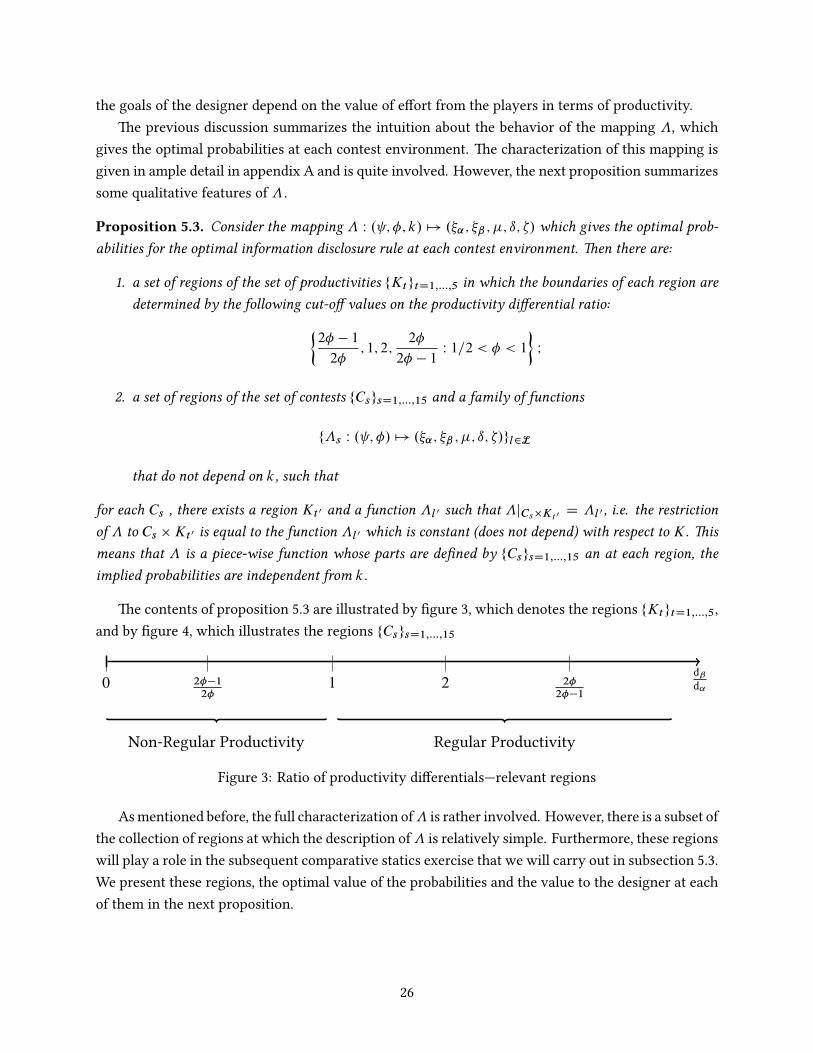
Proposition 5.3. Consider the mapping � W . ; �; k/ 7! .�˛; �ˇ ; �; ı; �/ which gives the optimal prob-abilities for the optimal information disclosure rule at each contest environment. Then there are:

1. a set of regions of the set of productivities fKtgtD1;:::;5 in which the boundaries of each region aredetermined by the following cut-off values on the productivity differential ratio:�

2� � 1

2�; 1; 2;

2�

2� � 1W 1=2 < � < 1

�I

2. a set of regions of the set of contests fCsgsD1;:::;15 and a family of functions

f�s W . ; �/ 7! .�˛; �ˇ ; �; ı; �/gl2L

that do not depend on k, such that

for each Cs , there exists a region Kt 0 and a function �l 0 such that �jCs�Kt0 D �l 0 , i.e. the restrictionof � to Cs �Kt 0 is equal to the function �l 0 which is constant (does not depend) with respect to K. Thismeans that � is a piece-wise function whose parts are defined by fCsgsD1;:::;15 an at each region, theimplied probabilities are independent from k.

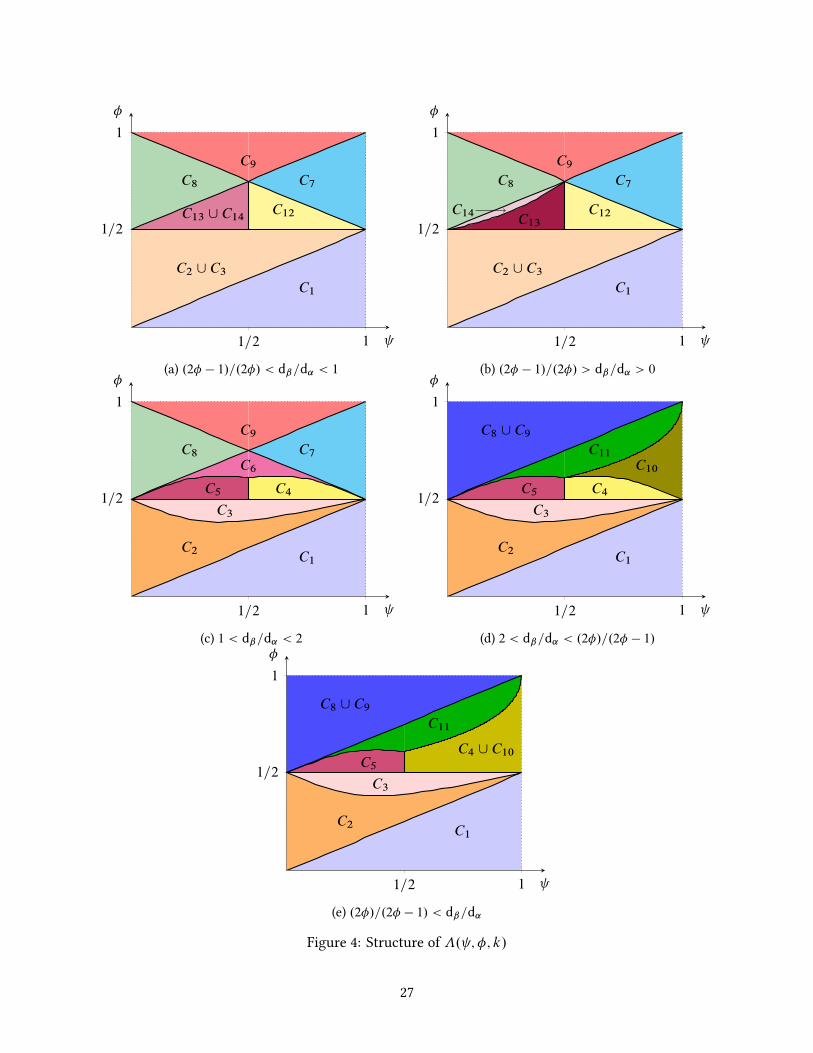
The contents of proposition 5.3 are illustrated by figure 3, which denotes the regions fKtgtD1;:::;5,and by figure 4, which illustrates the regions fCsgsD1;:::;15

dˇ

d˛0 2��1

2�1 2 2�

2��1

Non-Regular Productivity Regular Productivity

Figure 3: Ratio of productivity differentials—relevant regions

Asmentioned before, the full characterization of� is rather involved. However, there is a subset ofthe collection of regions at which the description of� is relatively simple. Furthermore, these regionswill play a role in the subsequent comparative statics exercise that we will carry out in subsection 5.3.We present these regions, the optimal value of the probabilities and the value to the designer at eachof them in the next proposition.

26

1=2 1

1=2

1

C1

C2 [ C3

C12C13 [ C14

C7C8

C9

�

(a) .2� � 1/=.2�/ < dˇ=d˛ < 1

1=2 1

1=2

1

C1

C2 [ C3

C12C13

C7C8

C9

C14

�

(b) .2� � 1/=.2�/ > dˇ=d˛ > 0

1=2 1

1=2

1

C1C2

C3

C4C5

C6

C7C8

C9

�

(c) 1 < dˇ=d˛ < 2

1=2 1

1=2

1

C1C2

C3

C4C5

C8 [ C9

C10

C11

�

(d) 2 < dˇ=d˛ < .2�/=.2� � 1/

1=2 1

1=2

1

C1C2

C3

C5

C8 [ C9

C4 [ C10

C11

�

(e) .2�/=.2� � 1/ < dˇ=d˛

Figure 4: Structure of �. ; �; k/

27

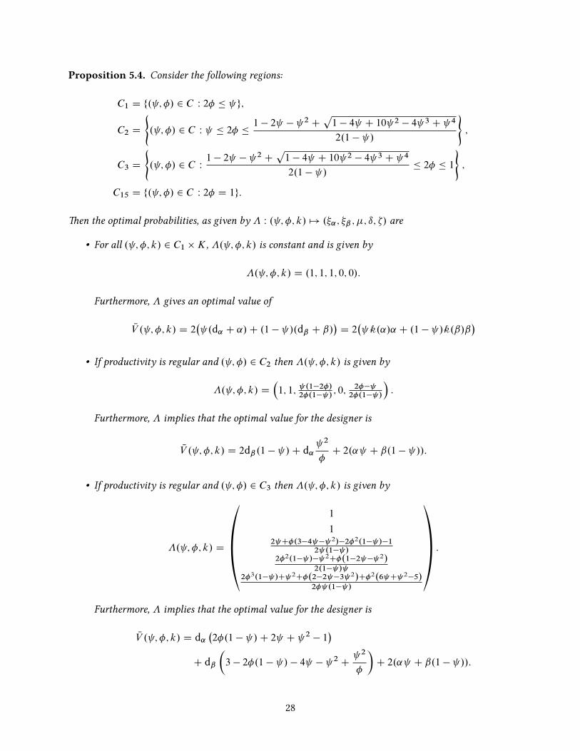
Proposition 5.4. Consider the following regions:

C1 D f. ; �/ 2 C W 2� � g;

C2 D

(. ; �/ 2 C W � 2� �

1 � 2 � 2 Cp1 � 4 C 10 2 � 4 3 C 4

2.1 � /

);

C3 D

(. ; �/ 2 C W

1 � 2 � 2 Cp1 � 4 C 10 2 � 4 3 C 4

2.1 � /� 2� � 1

);

C15 D f. ; �/ 2 C W 2� D 1g:

Then the optimal probabilities, as given by � W . ; �; k/ 7! .�˛; �ˇ ; �; ı; �/ are

• For all . ; �; k/ 2 C1 �K, �. ; �; k/ is constant and is given by

�. ; �; k/ D .1; 1; 1; 0; 0/:

Furthermore, � gives an optimal value of

NV . ; �; k/ D 2� .d˛ C ˛/C .1 � /.dˇ C ˇ/

�D 2

� k.˛/˛ C .1 � /k.ˇ/ˇ

�• If productivity is regular and . ; �/ 2 C2 then �. ; �; k/ is given by

�. ; �; k/ D

�1; 1; .1�2�/

2�.1� /; 0; 2��

2�.1� /

�:

Furthermore, � implies that the optimal value for the designer is

NV . ; �; k/ D 2dˇ .1 � /C d˛ 2

�C 2.˛ C ˇ.1 � //:

• If productivity is regular and . ; �/ 2 C3 then �. ; �; k/ is given by

�. ; �; k/ D

�1

12 C�.3�4 � 2/�2�2.1� /�1

2 .1� /2�2.1� /� 2C�.1�2 � 2/

2.1� / 2�3.1� /C 2C�.2�2 �3 2/C�2.6 C 2�5/

2� .1� /

�

:

Furthermore, � implies that the optimal value for the designer is

NV . ; �; k/ D d˛�2�.1 � /C 2 C 2 � 1

�C dˇ

�3 � 2�.1 � / � 4 � 2 C

2

�

�C 2.˛ C ˇ.1 � //:

28

• If productivity is non-regular and . ; �/ 2 C2 [ C3 then �. ; �; k/ is given by

�. ; �; k/ D

�1; 1; 2�

2�2�3C �3� C�2 2�.1� /

; �.2�� /2.1� /

; .1��/2.2�� /2�.1� /

:�

Furthermore, � implies that the optimal value for the designer is

NV . ; �; k/ D dˇ�2 � 2.1C �/ C 2

�C d˛

�2� � 2 C

2

�

�C 2.˛ C ˇ.1 � //:

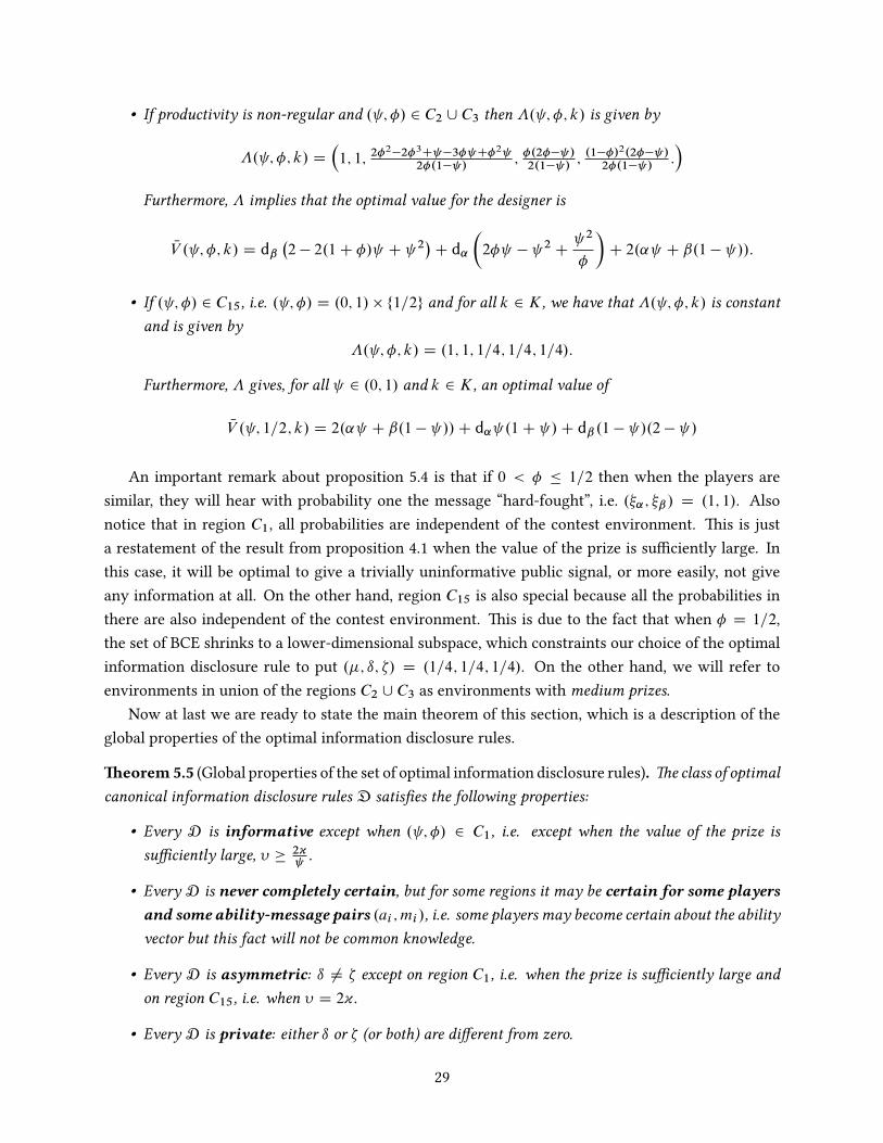
• If . ; �/ 2 C15, i.e. . ; �/ D .0; 1/ � f1=2g and for all k 2 K, we have that �. ; �; k/ is constantand is given by

�. ; �; k/ D .1; 1; 1=4; 1=4; 1=4/:

Furthermore, � gives, for all 2 .0; 1/ and k 2 K, an optimal value of

NV . ; 1=2; k/ D 2.˛ C ˇ.1 � //C d˛ .1C /C dˇ .1 � /.2 � /

An important remark about proposition 5.4 is that if 0 < � � 1=2 then when the players aresimilar, they will hear with probability one the message “hard-fought”, i.e. .�˛; �ˇ / D .1; 1/. Alsonotice that in region C1, all probabilities are independent of the contest environment. This is justa restatement of the result from proposition 4.1 when the value of the prize is sufficiently large. Inthis case, it will be optimal to give a trivially uninformative public signal, or more easily, not giveany information at all. On the other hand, region C15 is also special because all the probabilities inthere are also independent of the contest environment. This is due to the fact that when � D 1=2,the set of BCE shrinks to a lower-dimensional subspace, which constraints our choice of the optimalinformation disclosure rule to put .�; ı; �/ D .1=4; 1=4; 1=4/. On the other hand, we will refer toenvironments in union of the regions C2 [ C3 as environments with medium prizes.

Now at last we are ready to state the main theorem of this section, which is a description of theglobal properties of the optimal information disclosure rules.

Theorem5.5 (Global properties of the set of optimal information disclosure rules). The class of optimalcanonical information disclosure rules D satisfies the following properties:

• Every D is informative except when . ; �/ 2 C1, i.e. except when the value of the prize issufficiently large, � �

2~ .

• Every D is never completely certain, but for some regions it may be certain for some playersand some ability-message pairs .ai ; mi /, i.e. some players may become certain about the abilityvector but this fact will not be common knowledge.

• Every D is asymmetric: ı ¤ � except on region C1, i.e. when the prize is sufficiently large andon region C15, i.e. when � D 2~.

• Every D is private: either ı or � (or both) are different from zero.

29

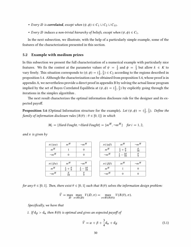
• Every D is correlated, except when . ; �/ 2 C1 [ C2 [ C15.

• Every D induces a non-trivial hierarchy of beliefs, except when . ; �/ 2 C1.

In the next subsection, we illustrate, with the help of a particularly simple example, some of thefeatures of the characterization presented in this section.

5.2 Example with medium prizes

In this subsection we present the full characterization of a numerical example with particularly nicefeatures. We fix the contest at the parameter values of D

12

and � D13

but allow k 2 K tovary freely. This situation corresponds to . ; �/ D .1

2; 13/ 2 C2 according to the regions described in

proposition 5.4. Although the characterization can be obtained from proposition 5.4, whose proof is inappendix A, we nevertheless provide a direct proof in appendix B by solving the actual linear programimplied by the set of Bayes Correlated Equilibria at . ; �/ D .1

2; 13/ by explicitly going through the

iterations in the simplex algoritihm .The next result characterizes the optimal information disclosure rule for the designer and its ex-

pected payoff.

Proposition 5.6 (Optimal Information structure for the example). Let . ; �/ D .12; 13/. Define the

family of information disclosure rules fS.�/ W � 2 Œ0; 1�g in which

Mi D fHard-Fought;:Hard-Foughtg D fmH ;:mH g for i D 1; 2,

and � is given by

�.�j˛˛/ mH :mH

mH 1 0

:mH 0 0

�.�j˛ˇ/ mH :mH

mH 12 C

�9

�18

:mH 12 �

5�18

�9

�.�jˇ˛/ mH :mH

mH 12 C

�9

12 �

5�18

:mH �18

�9

�.�jˇˇ/ mH :mH

mH 1 0

:mH 0 0

for any � 2 Œ0; 1�. Then, there exist � 2 Œ0; 1� such that S.�/ solves the information design problem:

xV D maxD

max�2E.D/

V.D ; �/ D max�2E.S.�//

V.S.�/; �/:

Specifically, we have that

1. If dˇ > d˛ then S.0/ is optimal and gives an expected payoff of

xV D ˛ C ˇ C3

4d˛ C dˇ (5.1)

30

2. If dˇ < d˛ then S.1/ is optimal and gives an expected payoff of

xV D ˛ C ˇ C5

6d˛ C

11

12dˇ : (5.2)

3. If dˇ D d˛ , then for any � 2 Œ0; 1�, the rule S.�/ is optimal and gives an expected payoff of

xV D ˛ C ˇ C7

4dˇ : (5.3)

Example 5.1. We will illustrate proposition (5.6) by specifying some values for the productivities ofthe players for each case.

1. ˛ D 3; ˇ D 4; k.˛/˛ D 5; k.ˇ/ˇ D 7. In this case we have that dˇ

d˛D

32. Thus

xV D23

2> V.C/ D

65

6> V.N / D

59

6:

2. ˛ D 3; ˇ D 4; k.˛/˛ D 5; k.ˇ/ˇ D 5:5. In this case we have that dˇ

d˛

34. Thus

xV D241

24> V.C/ D

115

12> V.N / D

103

12:

3. ˛ D 3; ˇ D 4; k.˛/˛ D 5; k.ˇ/ˇ D 6. In this case we have that dˇ

d˛D 1. Thus

xV D21

2> V.C/ D 10 > V.N / D 9

J

In the information design problem, it is important to remark again that for any information dis-closure rule, we are analyzing the equilibrium behavior that it engenders and then choosing the bestequilibrium from the point of view of the designer, as pointed out in section 2.1. We can see this intheorem 5.6 by noticing that to compute the expected payoff of the designer for the optimal rule S.�/,we are taking the maximum over the equilibrium set E.S.�// of the incomplete information gameinduced by S.�/. Therefore, what our results imply is that at least one equilibrium of E.S.�// will bethe optimal from the perspective of the designer. However, up until this point our results are silentabout the behavior of other equilibria in the equilibrium set.

5.2.1 Calculating the hiearchies of beliefs and Characterizing equilibrium set

The optimal information structure S.�/ induces a Bayesian Game, which we denote �S.�/. The equi-librium set of �S.�/ is denoted as E.S.�//. In light of the discussion at the end of the previousparagraph, it is important to obtain the full characterization of the equilibrium set to fully under-

31

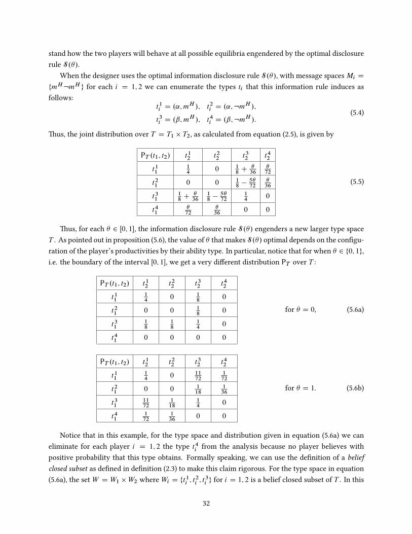
stand how the two players will behave at all possible equilibria engendered by the optimal disclosurerule S.�/.

When the designer uses the optimal information disclosure rule S.�/, with message spacesMi D

fmH:mH g for each i D 1; 2 we can enumerate the types ti that this information rule induces asfollows:

t1i D .˛;mH /; t2i D .˛;:mH /;

t3i D .ˇ;mH /; t4i D .ˇ;:mH /:(5.4)

Thus, the joint distribution over T D T1 � T2, as calculated from equation (2.5), is given by

PT .t1; t2/ t12 t22 t32 t42

t1114

0 18

C�36

�72

t21 0 0 18

�5�72

�36

t3118

C�36

18

�5�72

14

0

t41�72

�36

0 0

(5.5)

Thus, for each � 2 Œ0; 1�, the information disclosure rule S.�/ engenders a new larger type spaceT . As pointed out in proposition (5.6), the value of � that makes S.�/ optimal depends on the configu-ration of the player’s productivities by their ability type. In particular, notice that for when � 2 f0; 1g,i.e. the boundary of the interval Œ0; 1�, we get a very different distribution PT over T :

PT .t1; t2/ t12 t22 t32 t42

t1114

0 18

0

t21 0 0 18

0

t3118

18

14

0

t41 0 0 0 0

for � D 0, (5.6a)

PT .t1; t2/ t12 t22 t32 t42

t1114

0 1172

172

t21 0 0 118

136

t311172

118

14

0

t41172

136

0 0

for � D 1. (5.6b)

Notice that in this example, for the type space and distribution given in equation (5.6a) we caneliminate for each player i D 1; 2 the type t4i from the analysis because no player believes withpositive probability that this type obtains. Formally speaking, we can use the definition of a beliefclosed subset as defined in definition (2.3) to make this claim rigorous. For the type space in equation(5.6a), the set W D W1 �W2 where Wi D ft1i ; t

2i ; t

3i g for i D 1; 2 is a belief closed subset of T . In this

32

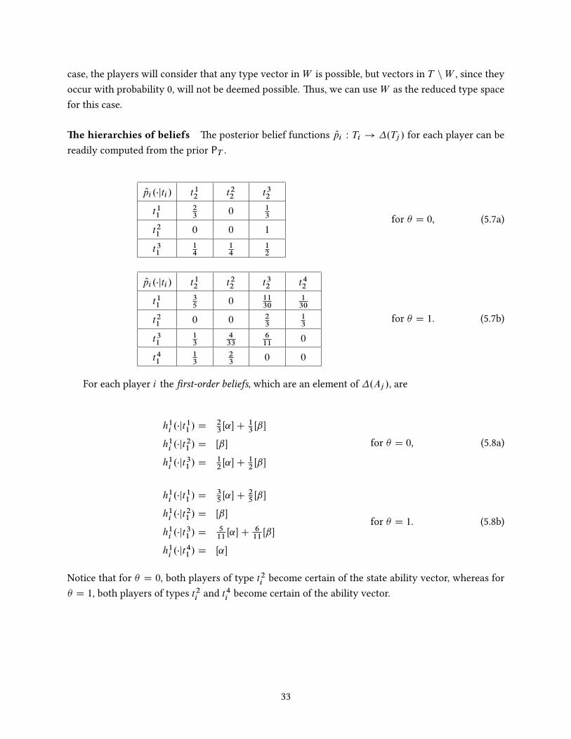
case, the players will consider that any type vector in W is possible, but vectors in T nW , since theyoccur with probability 0, will not be deemed possible. Thus, we can use W as the reduced type spacefor this case.

The hierarchies of beliefs The posterior belief functions Opi W Ti ! �.Tj / for each player can bereadily computed from the prior PT .

Opi .�jti / t12 t22 t32

t1123

0 13

t21 0 0 1

t3114

14

12

for � D 0, (5.7a)

Opi .�jti / t12 t22 t32 t42

t1135

0 1130

130

t21 0 0 23

13

t3113

433

611

0

t4113

23

0 0

for � D 1. (5.7b)

For each player i the first-order beliefs, which are an element of �.Aj /, are

h1i .�jt11 / D

23Œ˛�C 1

3Œˇ�

h1i .�jt21 / D Œˇ�

h1i .�jt31 / D

12Œ˛�C 1

2Œˇ�

for � D 0, (5.8a)

h1i .�jt11 / D

35Œ˛�C 2

5Œˇ�

h1i .�jt21 / D Œˇ�

h1i .�jt31 / D

511Œ˛�C 6

11Œˇ�

h1i .�jt41 / D Œ˛�

for � D 1. (5.8b)

Notice that for � D 0, both players of type t2i become certain of the state ability vector, whereas for� D 1, both players of types t2i and t4i become certain of the ability vector.

33

For each player i the second-order beliefs are, which are an element of �.Aj ��.Ai //, are

h2i .�jt11 / D

23Œ.˛; 2

3Œ˛�C 1

3Œˇ�/�C 1

3Œ.ˇ; 1

2Œ˛�C 1

2Œˇ�/�

h2i .�jt21 / D Œ.ˇ; 1

2Œ˛�C 1

2Œˇ�/�

h2i .�jt31 / D

14Œ.˛; 2

3Œ˛�C 1

3Œˇ�/�C 1

4Œ.˛; Œˇ�/�C 1

2Œ.ˇ; 1

2Œ˛�C 1

2Œˇ�/�

for � D 0, (5.9a)

h2i .�jt11 / D

35Œ.˛; Œˇ�/�C 11

30Œ.ˇ; 5

11Œ˛�C 6

11Œˇ�/�C 1

30Œ.ˇ; Œ˛�/�

h2i .�jt21 / D

23Œ.ˇ; 5

11Œ˛�C 6

11Œˇ�/�C 1

3Œ.ˇ; Œ˛�/�

h2i .�jt31 / D

13Œ.˛; 3

5Œ˛�C 2

5Œˇ�/�C 4

33Œ.˛; Œˇ�/�C 6

11Œ.ˇ; 5

11Œ˛�C 6

11Œˇ�/�

h2i .�jt41 / D

13Œ.˛; 3

5Œ˛�C 2

5Œˇ�/�C 2

3Œ.˛; Œˇ�/�

for � D 1. (5.9b)

The infinite hierarchy for each player i can be computed in a similar way by iterating the con-structions using the posterior beliefs function Opi as shown in subsection 2.3.2.

Notice that although both players at some types became certain of the state given their first-orderbeliefs, this fact didn’t became common knowledge, as can be seen from the second-order hierarchies.In particular, it is at states in which the players are different when they have the possibility of be-coming certain of this fact. However, this should not be commonly known. It is precisely for thisreason that public information disclosure rules, as the complete information rule or p; q rule, are notoptimal. In order to incentivize the players when they are different to work, the designer needs toselectively inform them with some probability. However, this needs to be done privately. It is crucialto have private information because in that way the designer can generate some asymmetry at thehigher-order hierarchies, which is needed for the players to work with higher probability when theyare different.

The equilibrium set We will focus on symmetric equilibria. The following two propositions char-acterize the symmetric BNE sets for the cases � D f0; 1g.

Proposition 5.7. Let � D 0 so that the optimal information disclosure rule is given by S.0/. For each i ,let �i .ti / 2 Œ0; 1� denote the probability putting effort when player i is of type ti . Let �i D .�i .t

ki //kD1;:::;3

denote the strategy vector of player i . The set of symmetric BNE for this optimal information disclosurerule is given by

E.S.0// D f� D .�1; �2/ W �i .t1i / 2 Œ

1

3; 1�; �i .t

2i / D 0; �i .t

3i / D 1; i D 1; 2:g (5.10)

The unique pure-strategy equilibrium profile ��, where ��i D .1; 0; 1/ for each i D 1; 2 is the one that

achieves the optimal value for the designer, i.e. xV D V.S.0/; ��/. Furthermore, for each � 2 E.S.0//,V.S.0/; �/ > V.C/, i.e. each equilibrium profile in E.S.0// gives a larger utility for the designer thanthe complete information disclosure rule.

34

Proposition 5.8. Let � D 1 so that the optimal information disclosure rule is given by S.1/. For each i ,let �i .ti / 2 Œ0; 1� denote the probability putting effort when player i is of type ti . Let �i D .�i .t

ki //kD1;:::;4

denote the strategy vector of player i . Let Y D convf.0; 12/; . 2

11; 0/; .1; 0/g. Then the set of symmetric

BNE for this optimal information disclosure rule is given by

E.S.1// D˚� D .�1; �2/ W

��i .t

1i /; �i .t

2i /�

2 Y; �i .t3i / D 1; �i .t

4i / D 0; i D 1; 2:

(5.11)

The unique pure-strategy equilibrium profile ��, where ��i D .1; 0; 1; 0/ for each i D 1; 2 is the one

that achieves the optimal value for the designer, i.e. xV D V.S.1/; ��/. Furthermore, if we define QY D

convf.0; 12/; . 2

11; 0/g, then for each � 2 E.S.1// we have that

• If � satisfies that��i .t

1i /; �i .t

2i /�

2 Y n QY for each i D 1; 2 then V.S.1/; �/ > V.C/.

• If � satisfies that��i .t

1i /; �i .t

2i /�

2 QY for each i D 1; 2. then V.S.1/; �/ D V.C/.

5.3 Optimal design when the designer can alter the value of the prize

In this section, we use the results from subsection 5.1 to derive a comparative statics result which isquite pertinent in this context. We ask the question of whether information design is useful when thedesigner can alter the value of the prize � , or equivalently, alter the normalized cost of putting effort�:

The rationale for asking whether the designer can gain from information design when altering thevalue of the prize is two-fold. Firstly, we can think that the designer has no control over the beliefsof the players, embodied by , nor on the abilities as defined in k or the cost of putting effort. At theoutset of the game we can interpret the model as a situation in which the designer has no control overthe previous parameters. However, the designer has control not only over the information structureof the game via the disclosure rules but also on the value of the prize that he wishes to offer. Whathappens to the optimal information structure when the value of the prize changes is a very relevantcomparative statics exercise.

The second reason comes from the fact that in this model, in the absence of information design, asingle prize scheme is optimal. This follows from the result in Moldovanu and Sela (2001, Prop. 1, pp.547). However, the size of the bursar to be distributed via the prize has a strong impact on alteringincentives in the model we are considering as was shown in proposition 4.1. If the value of the prizecan be altered and this value is interpreted as a cost to the designer then it is important to know whatcan be gained through the design of an optimal information disclosure rule.

With the previous motivations in mind, we proceed to describe the profit maximization problemthat the designer will face when altering the value of the prize. When the value of the prize canbe moved, optimal revenues from the designer when designing information can be expressed as thevalue achieved from the optimal information disclosure rule. Thus, revenues can be expressed withthe help of equation (2.4) as

35

xV .�I ~; ; k/ D maxD

max�2E. ;~=�;D/

V.D ; � I ; ~=�; k/; (5.12)

where in xW now the remaining parameters .~; ; k/ that represent respectively the cost of puttingeffort, the beliefs of the players and the designer and the productivity vector should be considered asparameters. On the other hand, the cost of altering the prize is only the size of the bursar that sucha prize represents, i.e. � .

Therefore, profits are revenues minus costs, ˘.�I ~; ; k/ D xV .�I ~; ; k/� �: Optimal profits arethus

˘�.~; ; k/ D sup�2.~;1/

f xV .�I ~; ; k/ � �g: (5.13)

Notice that in equation (5.13), the supremum is taken over the interval .~;1/ since this is in concor-dance with the restriction that 0 < � D ~=� < 1 discussed in section 2.

The next proposition follows trivially from proposition 4.1

Proposition 5.9. Maximal revenues are achieved when O� D 2~= and remain constant for any prizegreater than O� and for all ~; and k 2 K. Furthermore, the value xV . O�; ~; ; k/ is achieved by the nullinformation disclosure rule.

The simple reason for the statement in proposition 5.9 is that at values greater or equal to O� , wehave that it becomes a dominant strategy to work at all possible states under null information. Thus,in terms of revenues, xV . O�; ~; ; k/ is the upper bound that we can achieve when altering the prize andunder the possibility of designing information, since the optimal disclosure rule can involve sayingnothing to the players.

However, as ~ changes we have that

@ O�

@~D2

> 2:

Therefore, an increase in ~ needs an increase in the prize by more than two-fold to achieve theupper bound in revenues. In particular, when the probability that each player ascribes to their rivalbeing weak, , tends to zero, the value of the prize that is needed grows without bound. Hence, avery large prize may not be optimal since its benefits may not outweigh its costs. It may be the casethat a much smaller prize can be better under an optimal information disclosure rule.

On the other hand, we have that as changes

@ O�

@ D �

2~

2< 0;

so we have that when the players believe with high probability that their rival is weak, the value ofthe prize required to achieve the upper bound in revenue decreases.

From the discussion above it follows that we will need to compare the performance of the nullinformation scheme given by˘. O�I ~; ; k/ D xV . O�I ~; ; k/� O� to any other different scheme that we

36

are considering. In summary,˘. O�I ~; ; k/ provides the threshold on � at which the null informationdisclosure rule can become optimal if such value is equal to the supremum in equation (5.13). There-fore, we will look for conditions on the remaining parameters .~; ; k/ which imply an optimal prizeless than O�:

For a clean statement of the results, define L W .0; 1/ ! R as

L. / D 1 � 2 C 3 2 C

q1 � 4 C 10 2 � 4 3 C 4: (5.14)

The function L. / represents the boundary of a region, as a function of the beliefs of the players ,that the remaining parameters ~ and k need to satisfy in order for information design to be optimal atprize values lower than the one implied O� where the optimal information rule involves saying nothingto the players.

The results are presented in the next two theorems. Theorem 5.10 deals with the parameter condi-tions at which the optimal disclosure rule involves non-trivial communication with the players. The-orem 5.11 complements the previous theorem by describing the optimal disclosure rules that achievethe optimal profits.

Theorem 5.10. If productivity is regular we have that

1. If the parameters .~; ; k/ satisfy the condition: 0 < ~�d˛ 2 �

�dˇ�d˛

4

�L. /; then the optimal

prize scheme is

��D

4~.1 � /

L. / � 4 2< O�: (5.15)

2. If the parameters .~; ; k/ satisfy the condition:�dˇ�d˛

4

�L. / � ~ � d˛ 2, then the optimal

prize scheme is��

D 2~ < O�: (5.16)

3. If the parameters .~; ; k/ satisfy the condition: ~ � d˛ 2 � 0, then the optimal prize scheme isO� .

If productivity is non-regular, then

4. If the parameters .~; ; k/ satisfy the condition: 0 < 2~ 2 < d˛Cdˇ , then the optimal prize scheme

is��

D 2~ < O�: (5.17)

5. If the parameters .~; ; k/ satisfy the condition: 2~ 2 � d˛ C dˇ then the optimal prize scheme is

O� .

In cases 1,2 and 4 we have that˘�.~; ; k/ D ˘.��; ~; ; k/ > ˘. O�I ~; ; k/: On the other hand, incases 3 and 5 we have that ˘�.~; ; k/ D ˘. O�I ~; ; k/:

Thus, as long as ~�d˛ 2 � 0 for regular productivity or 2~ 2 < d˛Cdˇ for non-regular productivity,

non-trivial information design is optimal.

37

Theorem 5.11. If the parameters satisfy the conditions ~ � d˛ 2 � 0 for regular productivity or 2~ 2 <

d˛Cdˇ for non-regular productivity then the optimal information disclosure rule D� D ..Mi /iD1;2; ��/

hasMifAggressive;Not Aggressiveg D fmA;:mAg for i D 1; 2,

and �� W A ! �.M/ is as follows:

• For the regular productivity case in which�dˇ�d˛

4

�L. / � ~ � d˛ 2 or the non-regular produc-

tivity case in which 0 < 2~ 2 < d˛ C dˇ (cases 2 and 4 in theorem 5.10 above) we have that

��.�j˛˛/ D ��.�jˇˇ/ D Œ.mH ; mH /�;

��.ej˛ˇ/ D ��.ejˇ˛/ D 1=4; 8m 2 M:

• For the regular productivity case in which�dˇ�d˛

4

�L. / � ~ � d˛ 2 (case 1 in theorem 5.10) we

have that

��.�j˛˛/ D ��.�jˇˇ/ D Œ.mH ; mH /�;

��.mH ; mH j˛ˇ/ D ��.mH ; mH jˇ˛/ D2

L. / � 4 2�

1 �

��.:mH ; mH j˛ˇ/ D ��.mH ;:mH jˇ˛/ D1

1 � �

2

L. / � 4 2

6 Concluding remarks

This paper analyzes how a designer can use information to manipulate the beliefs in a contest inwhich there is incomplete information about the abilities of the contestants. We found that the op-timal disclosure rules make the crucial distinction between public and private information and ingeneral always use partial revelation of information. In particular, we showed how private informa-tion generates asymmetric hierarchies of beliefs which are necessary for the designer to benefit frominformation design. We also performed a cost-benefit analysis of optimal information design rule byintroducing a “price for information” and taking advantage of the full characterization results that weprovided. We found that for a robust set of parameters, information design is the most cost-efficientway to manipulate the players to act following the interests of the contest designer.

Throughout the analysis of optimal information disclosure rules, we have assumed that the de-signer was able to pick an equilibrium t hat is to her liking from the equilibrium set engenderedby an information disclosure rule. This equilibrium selection criterion is embedded into the reve-lation principle-style argument that provides the foundation to use the notion of Bayes CorrelatedEquilibrium as a first step into computing the optimal information disclosure rule for the designer.Generically, the optimal information disclosure rules for contests identified by this method engendera continuum of equilibria. Although we showed within the context of a particular example that allequilibria engendered by such a rule perform at least as good as the complete information disclosure

38

rule from the point of view of the designer, it remains an important question if we can refine theseresults. An important question is to analyze the performance of optimal disclosure rules when werelax the optimistic equilibrium selection criterion for another one. In particular, we would like toknow what kind of optimal rules arise when we replace the optimistic attitude of the designer bya pessimistic one in which she now considers that the worst equilibrium is the one that is going tobe picked by the players. In this sense, for any disclosure rule that the designer is considering, thispessimistic criteria ensures that any equilibria in the equilibrium set engendered by the disclosurerules perform at least as good as the worst-case scenario.

Tied to the previous notion is the issue about uniqueness of equilibrium under a particular in-formation disclosure rule. In the paper we identified two information disclosure rules, the null andcomplete rules, that have unique Bayes Nash Equilibrium profiles generically. However, in generalthese rules were far from optimal. If the designer could find an information disclosure rule that per-formed better than these two and at the same time engendered a unique equilibrium profile, then shewould not need to worry about the possibility of other bad equilibrium arising under such a rule.

A general solution the this problem can be obtained by extending the techniques in Mathevetet al. (2016) to the case in which the players hold prior private information, just like they do in thecontests considered here. However, concurrent work to this paper shows that when the designer hasa pessimistic attitude, the candidate optimal rule that emerges turns out to be public. In particularthe optimal public information disclosure rule turns out to engender generically a unique equilibrium.This is in sharp contrast to the results of this paper and points out the value of public informationdisclosure in contests as a mean to incentivize unique equilibrium profiles. An open question remainsabout how general this statement is for other classes of games and designer’s objectives.

A second extension is the case of differential information between the designer and the playerswhile still satisfying the assumption of distributed knowledge between the players and the designer.When the designer also has private information, any choice of information disclosure rule runs therisk of informing the players about what the designer knows, and thus impacting the power of thedesigner to guide the players to her desire course of action. Therefore, further restrictions need tobe imposed on the choice of the information disclosure rule in order to counteract this effect. Thisconsideration ties in with the problem of the informed principal in the mechanism design literature.

A final extension that is interesting to analyze is the case of prior private information betweenthe players which does not satisfy the distributed knowledge requirement. For example, suppose thatthe incomplete information in the game is not only described by the ability vector, whose individualcomponents are assumed to be known privately by the players, but the uncertainty in the contestalso comes from a random component in the value of the prize of which the contestants only receivea partially correlated signal. A real-life situation that could be modeled by this environment wouldbe Research and Development races, in which the value of the invention is initially unknown to theplayers. In this case, a designer perhaps can disclose information about the value of the prize, thecontestants’ ability or both. In this case, although the techniques from Bergemann and Morris (2016)still apply, it is nevertheless too artificial since the designer would need to know information that the

39

players do not jointly possess.So, this is how the story ends. The hare never understood what happened that day. The fox, as a

designer, was the real winner. Now, we can extract a new moral from the famous fable: if you wantothers to behave as you wish, don’t say more than you need, and just wait until everything is on its stead.

40

A Finding anoptimal BayesCorrelated Equilibrium for theDesigner

A.1 Simplifying the BCE optimization program

In section 3 we described the steps in which the information design problem (2.4) could be simplifiedto the search of an optimal Bayes Correlated Equilibrium distribution � in view of theorem 3.2. Equa-tion (3.4) formalizes the previous claim by showing that the optimal value of the information designproblem es equivalent to the value given by the optimal BCE decision rule �.

For any . ; �/ 2 C , a decision rule � W A ! �.E/ as in definition 3.1 is a four-tuple whosecomponents come from the three-dimensional probability simplex simplex �3, i.e. � 2

Q4iD1�3 D

�43. Problem (3.4) is thus:

max�2�4

3

V.�/ (A.1)

subject to:Xej ;aj

prob.aj jai /�.ei ; ej ja/�Oui .ei ; ej ; a/ � Oui .e

0i ; ej ; a/

�� 0; (A.2)

8i; j D 1; 2; i ¤ j; 8ai 2 Ai ;8ei ; e0i 2 Ei ; ei ¤ e0

i :

There are some features that we wish to point out about the previous program. We have that�43 � R16. If � 2 �43, then it needs to satisfy four equality constraints that ensure that for each a 2 A,Pe2E �.eja/ D 1. Each one of the equality constraints can be represented by two paired inequality

constraints, for a total of 8. Furthermore, there are 16 non-negativity constraints, i.e. �.eja/ � 0 foreach a 2 A and e 2 E . Additionally the set of inequalities (A.2) describe the obedience constraintsimplied by the BCE concept, which is also linear in �. Furthermore we have jEi j�jAi j D 4 constraintsper player for a total of 8. Therefore the program has 32 inequality constraints in 16 variables. Theobjective (A.1) is linear in �. Using these observations, we conclude that the previous program is alinear programming problem.

The objective of this appendix is to provide the details on how to solve this program.First of all, notice that we can reduce the number of variables to consider by noticing that equality

constraints that define the four-fold product of the three dimensional simplex ensure that in �.�ja/one of the numbers is determined by the other three for each a 2 A, which would reduce the numberof variables to 12, with 4 inequality constraints representing the 4-fold probability simplices, 12 non-negativity constraints, and 8 obedience constraints for a total of 24 constraints.

To simplify further the problem and make it tractable for analysis, we will focus on symmetricBayes Correlated Equilibria, hereafter SBCE. It is obvious that SBCE � BCE, however, it will beshown that the optimal BCE for the designer actually occurs at a symmetric BCE. The set of SBCEcan be parameterized as shown in figure 5.

Let � D . ˛; �˛; ˇ ; �ˇ ; �; ı; �/| 2 R7 represent the parameterized decision rule .�.�ja//a2A 2 �43

as in figure 5. For this parameterization to be a valid system of conditional probability distributions

41

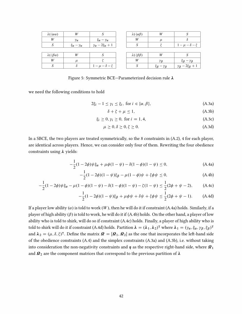
�.�j˛˛/ W S

W ˛ �˛ � ˛

S �˛ � ˛ ˛ � 2�˛ C 1

�.�j˛ˇ/ W S

W � ı

S � 1 � � � ı � �

�.�jˇ˛/ W S

W � �

S ı 1 � � � ı � �

�.�jˇˇ/ W S

W ˇ �ˇ � ˇ

S �ˇ � ˇ ˇ � 2�ˇ C 1

Figure 5: Symmetric BCE—Parameterized decision rule �

we need the following conditions to hold

2�i � 1 � i � �i ; for i 2 f˛; ˇg; (A.3a)ı C � C � � 1; (A.3b)

�i � 0; i � 0; for i D 1; 4, (A.3c)� � 0; ı � 0; � � 0: (A.3d)

In a SBCE, the two players are treated symmetrically, so the 8 constraints in (A.2), 4 for each player,are identical across players. Hence, we can consider only four of them. Rewriting the four obedienceconstraints using � yields:

�1

2.1 � 2�/ �˛ C ��.1 � / � ı.1 � �/.1 � / � 0; (A.4a)

�1

2.1 � 2�/.1 � /�ˇ � �.1 � �/ C �� � 0; (A.4b)

�1

2.1 � 2�/ �˛ � �.1 � �/.1 � / � ı.1 � �/.1 � / � �.1 � / �

1

2.2� C � 2/; (A.4c)

�1

2.1 � 2�/.1 � /�ˇ C �� C ı C �� �

1

2.2� C � 1/: (A.4d)

If a player low ability .˛/ is told to work .W /, then he will do it if constraint (A.4a) holds. Similarly, if aplayer of high ability .ˇ/ is told to work, he will do it if (A.4b) holds. On the other hand, a player of lowability who is told to shirk, will do so if constraint (A.4c) holds. Finally, a player of high ability who istold to shirk will do it if constraint (A.4d) holds. Partition � D .�1;�2/

| where �1 D . ˛; �˛; ˇ ; �ˇ /|

and �2 D .�; ı; �/|. Define the matrix ˝ D Œ˝1;˝2� as the one that incorporates the left-hand sideof the obedience constraints (A.4) and the simplex constraints (A.3a) and (A.3b), i.e. without takinginto consideration the non-negativity constraints and � as the respective right-hand side, where ˝1

and ˝2 are the component matrices that correspond to the previous partition of �

42

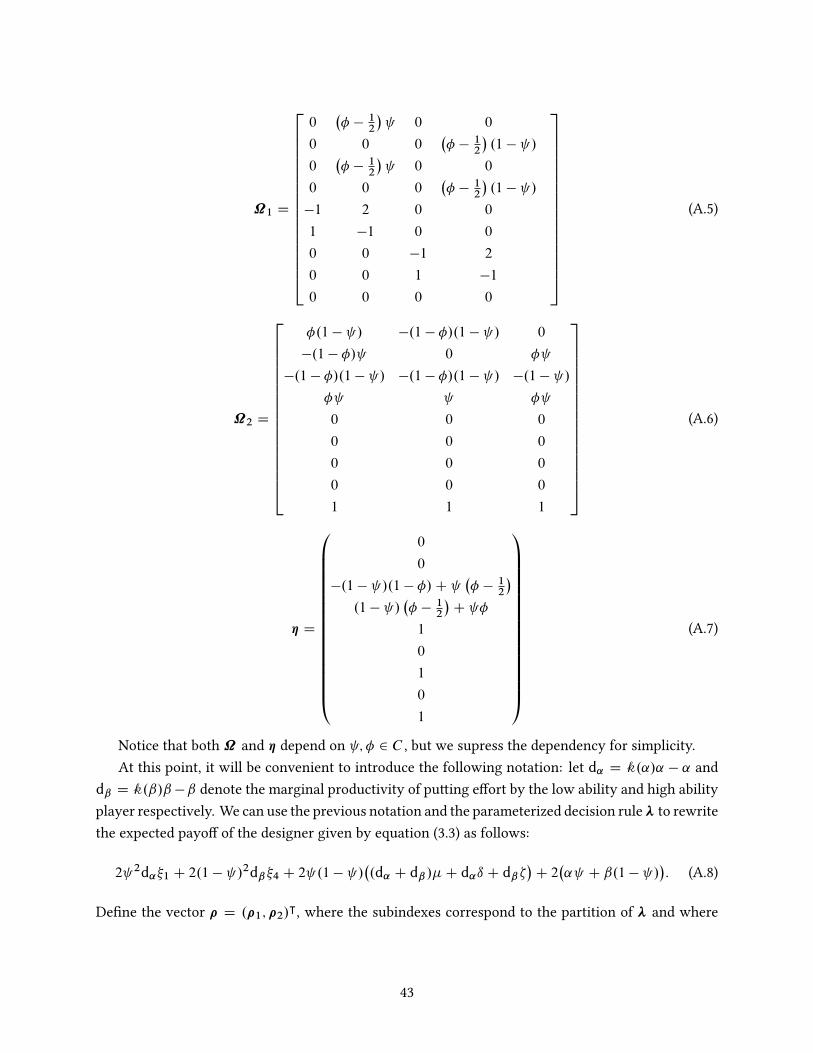
˝1 D

266666666666666664

0�� �

12

� 0 0

0 0 0�� �

12

�.1 � /

0�� �

12

� 0 0

0 0 0�� �

12

�.1 � /

�1 2 0 0

1 �1 0 0

0 0 �1 2

0 0 1 �1

0 0 0 0

377777777777777775(A.5)

˝2 D

266666666666666664

�.1 � / �.1 � �/.1 � / 0

�.1 � �/ 0 �

�.1 � �/.1 � / �.1 � �/.1 � / �.1 � /

� �

0 0 0

0 0 0

0 0 0

0 0 0

1 1 1

377777777777777775(A.6)

� D

0BBBBBBBBBBBBBBBB@

0

0

�.1 � /.1 � �/C �� �

12

�.1 � /

�� �

12

�C �

1

0

1

0

1

1CCCCCCCCCCCCCCCCA(A.7)

Notice that both ˝ and � depend on ; � 2 C , but we supress the dependency for simplicity.At this point, it will be convenient to introduce the following notation: let d˛ D k.˛/˛ � ˛ and

dˇ D k.ˇ/ˇ�ˇ denote the marginal productivity of putting effort by the low ability and high abilityplayer respectively. We can use the previous notation and the parameterized decision rule � to rewritethe expected payoff of the designer given by equation (3.3) as follows:

2 2d˛�1 C 2.1 � /2dˇ �4 C 2 .1 � /�.d˛ C dˇ /�C d˛ı C dˇ �

�C 2

�˛ C ˇ.1 � /

�: (A.8)

Define the vector � D .�1;�2/|, where the subindexes correspond to the partition of � and where

43

�1 D .0; 2d˛; 0; .1 � /2dˇ /| and �2 D .d˛ C dˇ ;d˛;dˇ /|. Then (A.8) can be written as

2�|1�1 C 2 .1 � /�

|2�2 C 2

�˛ C ˇ.1 � /

�: (A.9)

We conclude that the objective (A.1) subject to the set of constraints (A.2) is equivalent to thefollowing program.

NV D max�2R7

˚2�

|1�1 C 2 .1 � /�

|2�2 C 2

�˛ C ˇ.1 � /

�subject to

˝1�1 C ˝2�2 � � and� � 0:

(A.10)

Remark: NV also depends on . ; �; k/ but we suppress the dependency for simplicity. 16

A.2 Further simplifying reductions and auxiliary results

Inspection of the objective (A.9) and the obedience constraints (A.4) yields the following lemma,whose proof is trivial.

Lemma A.1. In an optimal SBCE for the designer, when the players are similar, the probability thatboth work, j and the probability that only one of them works, �j are equal, i.e. j D �j for j 2 f˛; �g.Thus, in an optimal SBCE, when the players are similar either they are both working or both shirking ormixing between these two cases.

Proof. Notice that j , j 2 f˛; �g does not enter into the objective (A.9) nor appears in the con-straints (A.4). The only place that these two variables appear is in the simplex constraints (A.3a)and the non-negativity constraints (A.3c). Thus, without loss of generality, we can put j D �j forj 2 f˛; �g without altering the optimal value of the problem and without affecting the rest of thefeasible set. �

Lemma A.1 yields the following corollaries.

Corollary A.2. The simplex constraints (A.3a) pertaining to the states when the players are similar, i.e.a 2 f˛˛; ˇˇg, can be compressed into the single constraints �j � 1 for j 2 f˛; ˇg:

Corollary A.3. Define the reduced vector O� D . O�1;�2/ where O�1 D .�˛; �ˇ /| and �2 D .�; ı; �/|

remains the same as before. Furthermore, define O� D . O�1;�2/| where O�1 D . 2d˛; .1 � /2dˇ /| and

�2 remains as before. Finally, define the partitioned matrix O D Œ O1; O

2� representing the reducedleft-hand side obedience constraints and the reduced vector O� of the corresponding right-hand side as

16Notation: if x; y 2 Rn:• x � y , xi � yi ; i D 1; : : : ; n:

• x > y , xi � yi ; i D 1; : : : ; n and x ¤ y :

• x � y , xi > yi ; i D 1; : : : ; n:

44

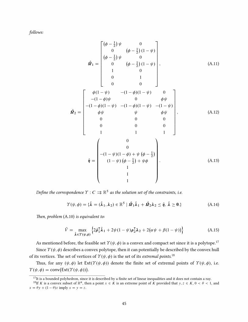
follows:

O1 D

2666666666664

�� �

12

� 0

0�� �

12

�.1 � /�

� �12

� 0

0�� �

12

�.1 � /

1 0

0 1

0 0

3777777777775; (A.11)

O2 D

2666666666664

�.1 � / �.1 � �/.1 � / 0

�.1 � �/ 0 �

�.1 � �/.1 � / �.1 � �/.1 � / �.1 � /

� �

0 0 0

0 0 0

1 1 1

3777777777775; (A.12)

O� D

0BBBBBBBBBBB@

0

0

�.1 � /.1 � �/C �� �

12

�.1 � /

�� �

12

�C �

1

1

1

1CCCCCCCCCCCA: (A.13)

Define the correspondence � W C � R5 as the solution set of the constraints, i.e.

� . ; �/ D f O� D . O�1;�2/ 2 R5 j O1

O�1 C O2�2 � O�; O� � 0:g (A.14)

Then, problem (A.10) is equivalent to:

NV D maxO�2� . ;�/

n2 O�

|1

O�1 C 2 .1 � /�|2�2 C 2

�˛ C ˇ.1 � /

�o(A.15)

As mentioned before, the feasible set � . ; �/ is a convex and compact set since it is a polytope.17

Since � . ; �/ describes a convex polytope, then it can potentially be described by the convex hullof its vertices. The set of vertices of � . ; �/ is the set of its extremal points.18

Thus, for any . ; �/ let Ext.� . ; �// denote the finite set of extremal points of � . ; �/, i.e.� . ; �/ D conv

�Ext.� . ; �//

�.

17It is a bounded polyhedron, since it is described by a finite set of linear inequalities and it does not contain a ray.18If K is a convex subset of Rn, then a point x 2 K is an extreme point of K provided that y; z 2 K, 0 < � < 1, and

x D �y C .1 � �/z imply x D y D z.

45

However, trying to search for all possible vertices of � . ; �/ is a daunting task, since we have thefollowing bounds (Salomone, Vaisman, and Kroese, 2016; Eckhoff, Gruber, and Wills, 1993):

1. By the McMullen upper bound theorem; the number of vertices jExt.� . ; �//j is at most n � b.d C 1/=2c

n � d

!C

n � b.d C 2/=2c

n � d

!D 2

12

7

!D 72;

where the number of half-spaces that define � . ; �/ is n D 12, since we have 7 inequalitiesplus 4 non-negativity constraints, and d D 5 since O� 2 R5.

2. By the Barnette lower bound theorem, the number of vertices jExt.� . ; �//j is at least

n.d � 1/ � .d C 1/.d � 2/ D 30;

where n and d are as before.

Thus, trying to find the set of extremal points of � . ; �/ for all . ; �/ 2 C , and then evaluate theobjective function at each of them in order to compare them is an intractable approach in general.

However, there is one situation in which we can completely describe � . ; �/ and that is when� D 1=2. The following lemma records this observation.

Lemma A.4. Let � D 1=2. Then, for any 2 .0; 1/, we have

� .. ; 1=2// D f O� 2 R5j0 � �˛ � 1; 0 � �ˇ � 1; � D ı D � D 1=4g:

Proof. We start by substituting � D 1=2 in O1, O

2 and O�. After the substitution, notice that the upperportion of O

1 vanishes, which implies that the only constraints affecting O�1 D .�˛; �ˇ / are 0 � �˛ � 1

and 0 � �ˇ � 1.On the other hand, we have after some simplifications the following constraints on �2 D .�; ı; �/

� � ı; (A.16a)� � �; (A.16b)

�� � ı � 2� � �1; (A.16c)�C 2ı C � � 1; (A.16d)�C ı C � � 1: (A.16e)

Inequalities (A.16a) and (A.16b) imply that � � � � ı. Adding up inequalities (A.16c) and (A.16d)yields ı � �. The previous two inequalities implies that � D ı D �, which together with (A.16e) andthe non-negativity constraints implies that these three numbers must equal 1=4, which concludes theproof.

�

46

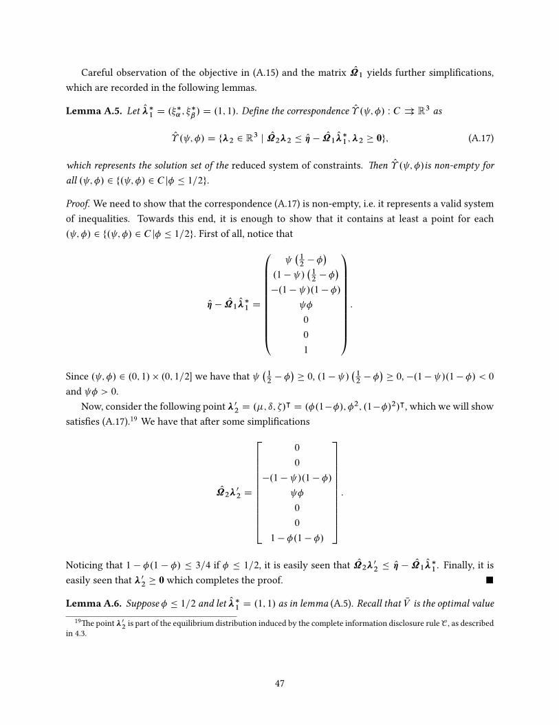
Careful observation of the objective in (A.15) and the matrix O1 yields further simplifications,

which are recorded in the following lemmas.

Lemma A.5. Let O��1 D .��

˛ ; ��ˇ/ D .1; 1/. Define the correspondence O� . ; �/ W C � R3 as

O� . ; �/ D f�2 2 R3 j O2�2 � O� � O

1O��1;�2 � 0g; (A.17)

which represents the solution set of the reduced system of constraints. Then O� . ; �/is non-empty forall . ; �/ 2 f. ; �/ 2 C j� � 1=2g.

Proof. We need to show that the correspondence (A.17) is non-empty, i.e. it represents a valid systemof inequalities. Towards this end, it is enough to show that it contains at least a point for each. ; �/ 2 f. ; �/ 2 C j� � 1=2g: First of all, notice that

O� � O1

O��1 D

0BBBBBBBBBBB@

�12

� ��

.1 � /�12

� ��

�.1 � /.1 � �/

�

0

0

1

1CCCCCCCCCCCA:

Since . ; �/ 2 .0; 1/ � .0; 1=2� we have that �12

� ��

� 0, .1� /�12

� ��

� 0, �.1� /.1� �/ < 0

and � > 0.Now, consider the following point �0

2 D .�; ı; �/| D .�.1��/; �2; .1��/2/|, which we will showsatisfies (A.17).19 We have that after some simplifications

O2�

02 D

2666666666664

0

0

�.1 � /.1 � �/

�

0

0

1 � �.1 � �/

3777777777775:

Noticing that 1 � �.1 � �/ � 3=4 if � � 1=2, it is easily seen that O2�

02 � O� � O

1O��1 . Finally, it is

easily seen that �02 � 0 which completes the proof. �

Lemma A.6. Suppose � � 1=2 and let O��1 D .1; 1/ as in lemma (A.5). Recall that NV is the optimal value

19The point �02 is part of the equilibrium distribution induced by the complete information disclosure rule C , as described

in 4.3.

47

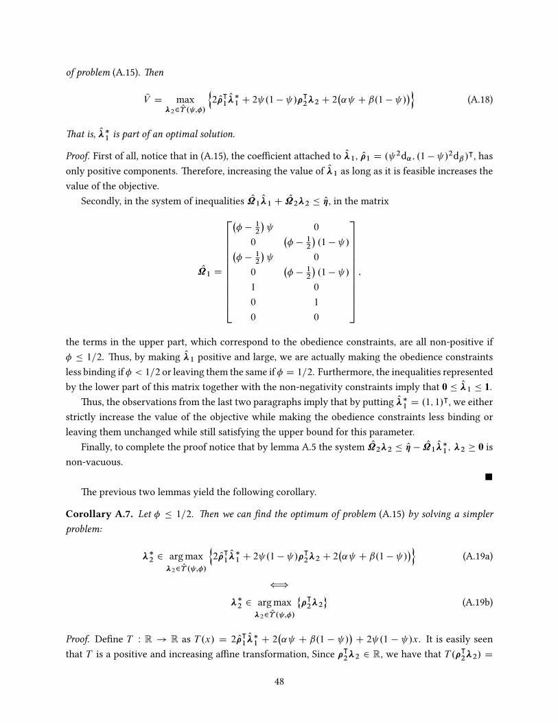
of problem (A.15). Then

NV D max�22 O� . ;�/

n2 O�

|1

O��1 C 2 .1 � /�

|2�2 C 2

�˛ C ˇ.1 � /

�o(A.18)

That is, O��1 is part of an optimal solution.

Proof. First of all, notice that in (A.15), the coefficient attached to O�1, O�1 D . 2d˛; .1 � /2dˇ /|, hasonly positive components. Therefore, increasing the value of O�1 as long as it is feasible increases thevalue of the objective.

Secondly, in the system of inequalities O1

O�1 C O2�2 � O�, in the matrix

O1 D

2666666666664

�� �

12

� 0

0�� �

12

�.1 � /�

� �12

� 0

0�� �

12

�.1 � /

1 0

0 1

0 0

3777777777775;

the terms in the upper part, which correspond to the obedience constraints, are all non-positive if� � 1=2. Thus, by making O�1 positive and large, we are actually making the obedience constraintsless binding if � < 1=2 or leaving them the same if � D 1=2. Furthermore, the inequalities representedby the lower part of this matrix together with the non-negativity constraints imply that 0 � O�1 � 1.

Thus, the observations from the last two paragraphs imply that by putting O��1 D .1; 1/|, we either

strictly increase the value of the objective while making the obedience constraints less binding orleaving them unchanged while still satisfying the upper bound for this parameter.

Finally, to complete the proof notice that by lemma A.5 the system O2�2 � O� � O

1O��1; �2 � 0 is

non-vacuous.�

The previous two lemmas yield the following corollary.

Corollary A.7. Let � � 1=2. Then we can find the optimum of problem (A.15) by solving a simplerproblem:

��2 2 argmax

�22 O� . ;�/

n2 O�

|1

O��1 C 2 .1 � /�

|2�2 C 2

�˛ C ˇ.1 � /

�o(A.19a)

”

��2 2 argmax

�22 O� . ;�/

˚�

|2�2

(A.19b)

Proof. Define T W R ! R as T .x/ D 2 O�|1

O��1 C 2

�˛ C ˇ.1 � /

�C 2 .1 � /x. It is easily seen

that T is a positive and increasing affine transformation, Since �|2�2 2 R, we have that T .�|

2�2/ D

48

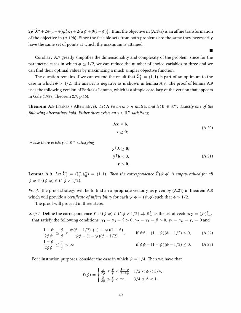
2 O�|1

O��1C2 .1� /�

|2�2C2

�˛ Cˇ.1� /

�. Thus, the objective in (A.19a) is an affine transformation

of the objective in (A.19b). Since the feasible sets from both problems are the same they necessarilyhave the same set of points at which the maximum is attained.

�Corollary A.7 greatly simplifies the dimensionality and complexity of the problem, since for the

parametric cases in which � � 1=2, we can reduce the number of choice variables to three and wecan find their optimal values by maximizing a much simpler objective function.

The question remains if we can extend the result that O��1 D .1; 1/ is part of an optimum to the

case in which � > 1=2. The answer is negative as is shown in lemma A.9. The proof of lemma A.9uses the following version of Farkas’s Lemma, which is a simple corollary of the version that appearsin Gale (1989, Theorem 2.7, p.46).

Theorem A.8 (Farkas’s Alternative). Let A be an m � n matrix and let b 2 Rm. Exactly one of thefollowing alternatives hold. Either there exists an x 2 Rn satisfying

Ax � b;

x � 0I(A.20)

or else there exists y 2 Rm satisfyingy|A � 0;

y|b < 0;

y > 0:

(A.21)

Lemma A.9. Let O��1 D .��

˛ ; ��ˇ/ D .1; 1/. Then the correspondence O� . ; �/ is empty-valued for all

; � 2 f. ; �/ 2 C j� > 1=2g.

Proof. The proof strategy will be to find an appropriate vector y as given by (A.21) in theorem A.8which will provide a certificate of infeasibility for each ; � D . ; �/ such that � > 1=2:

The proof will proceed in three steps.

Step 1. Define the correspondence Y W f. ; �/ 2 C j� > 1=2g � R7C as the set of vectors y D .yi /7iD1

that satisfy the following conditions: y1 D y3 D Oy > 0; y2 D y4 D Qy > 0; y5 D y6 D y7 D 0 and

1 �

2� �

Qy

Oy< .� � 1=2/C .1 � /.1 � �/

� � .1 � /.� � 1=2/; if � � .1 � /.� � 1=2/ > 0; (A.22)

1 �

2� �

Qy

Oy< 1 if � � .1 � /.� � 1=2/ � 0: (A.23)

For illustration purposes, consider the case in which D 1=4. Then we have that

Y.�/ D

˚32�

�QyOy< 5�4�3�4�

1=2 < � < 3=4;

32�

�QyOy< 1 3=4 � � < 1:

49

1=2 3=4 1

3=2

3

�

Qy

Oy

Figure 6: The correspondence Y.�/, when D 1=2 in .�; Qy= Oy/-space.

Figure 6 plots the correspondence in .�; Qy= Oy/-space.

We need to show that Y. ; �/ is well-defined and non-empty valued for all ; � 2 f. ; �/ 2 C j� >

1=2g: Notice that since � > 1=2

1 �

2� >1 �

> 0 )

Qy

Oy> 0:

The expression .� � 1=2/C .1 � /.1 � �/

� � .1 � /.� � 1=2/;

has a positive numerator since � > 1=2: Furthermore, if the denominator is positive, i.e. � � .1�

/.��1=2/ > 0, then the whole expression is strictly positive. If on the other hand the denominatoris strictly negative, i.e. � � .1 � /.� � 1=2/ < 0 then the whole expression is strictly negative.

We now show that if � � .1 � /.� � 1=2/ > 0 and � > 1=2, then

1 �

2� < .� � 1=2/C .1 � /.1 � �/

� � .1 � /.� � 1=2/; (A.24)

which makes the condition regarding Qy= Oy in (A.22) well-defined. The inequality in (A.24) is equiv-alent to

0 <

� .� � 1=2/C .1 � /.1 � �/

�2� �

� � � .1 � /.� � 1=2/

�.1 � /�

2 ��� � � .1 � /.� � 1=2/

� :

50

After some algebraic manipulations, the previous inequality es equivalent to

0 <

�� � 1=2

��2� 2 C .1 � /2

�� 2.1 � / �.� � 1=2/�

2 ��� � � .1 � /.� � 1=2/

�D.� � 1=2/

�2� .2 � 1/C .1 � /2

��2 �

�� � � .1 � /.� � 1=2/

� : (A.25)

In light of (A.25), we can see that inequality (A.24) is true if and only if the terms in parenthesisare either all strictly positive or strictly negative at the same time. Since by assumption 1=2 < � < 1,0 < < 1 so that � > 0, and � � .1 � /.� � 1=2/ > 0 we only need to check the sign of2� .2 � 1/C .1 � /2. We have that

2� .2 � 1/C .1 � /2 > .2 � 1/C .1 � /2 D 3 2 � 3 C 1 � 1=4 > 0; (A.26)

where the first inequality in (A.26) is due to the fact that � > 1=2 and the final inequality is dueto the fact that 3 2 � 3 C 1 is a convex function of which achieves its minimum at 1=4 when D 1=2.

Therefore, the previous arguments show that Y. ; �/ is a well-defined non-empty correspondence.

Fix any y 2 Y. ; �/. We will show that y provides a certificate of infeasibility. From theorem A.8we need the inequalities in (A.21) to hold:

y| O2 � 0; (A.27a)

y|. O� � O1

O��1/ < 0; (A.27b)y > 0: (A.27c)

Evidently, by step 2, each component of y is either zero or strictly positive so (A.27c) holds. From (A.27a)we get after rearranging and simplifying terms

y| O2 D

0B@ .2� � 1/�.1 � / Oy C Qy

��2�.1 � �/.1 � /

�Oy C Qy

�.1 � / Oy C 2� Qy

1CA|

� 0: (A.28)

Similarly, we get from (A.27b) after collecting terms and rearranging that

� Oy� .� � 1=2/C .1 � /.1 � �/

�C Qy

� � � .1 � /.� � 1=2/

�< 0: (A.29)

In (A.28), the first component is strictly positive because 0 < < 1 and 1=2 < � < 1, so this

51

inequality will not be binding. Thus, we need the following system to have a solution

Qy � 2�.1 � �/.1 � /

�; (A.30a)

2� Qy � .1 � / Oy; (A.30b)Qy� � � .1 � /.� � 1=2/

�< Oy

� .� � 1=2/C .1 � /.1 � �/

�: (A.30c)

The coefficients attached to Qy and Oy in inequalities (A.30a) and (A.30b) are strictly positive by as-sumption, so these two are equivalent to

max�2.1 � �/.1 � /

;.1 � /

2�

��

Qy

Oy(A.31)

Notice that in (A.31), the inequality

2.1 � �/.1 � /

<.1 � /

2� ,

4�.1 � �/ � 1

2� < 0 , 4�.1 � �/ < 1

holds since 0 < � < 1 and 4�.1 � �/ < 1 because � > 1=2.

On the other hand, in inequality (A.30c), the coefficient attached to Oy is strictly positive when� > 1=2 but the coefficient of Qy can change sign. If it is strictly positive, i.e. � �.1� /.��1=2/ > 0,then the inequality does provide an upper bound on Qy= Oy:

Qy

Oy< .� � 1=2/C .1 � /.1 � �/

� � .1 � /.� � 1=2/;

and provides no restriction in any other case, i.e. � � .1 � /.� � 1=2/ � 0.

Combining all these observations, we have that all of them correspond to the definition of Y. ; �/,and thus we have shown that the vector y that we arbitrarily chose indeed is a certificate of opti-mality. This concludes the proof.

�

A.3 Full characterization of the optimal SBCE

After all the work done to simplify the problem in the previous subsections, we are now ready tomove forward with the characterization of an optimal Symmetric Bayes Correlated Equilibrium.

Before proceeding there are a few remarks that are in order. We are looking to describe theset of optima of problem (A.10) as a function of all contests . ; �/ 2 C and all productivities k 2 K.Problem (A.10) is a parametric linear programming problem and although is structurally simple it stillposes a challenge to solve fully. The simplifications from the previous subsections in this appendixwill help in the full characterization. The search for an optimal solution involves making sure thatwe are finding positive solutions. On the other hand, the objective function depends on the marginalproductivities .d˛;dˇ /: Therefore, the structure and shape of the set of optimizers will be impacted

52

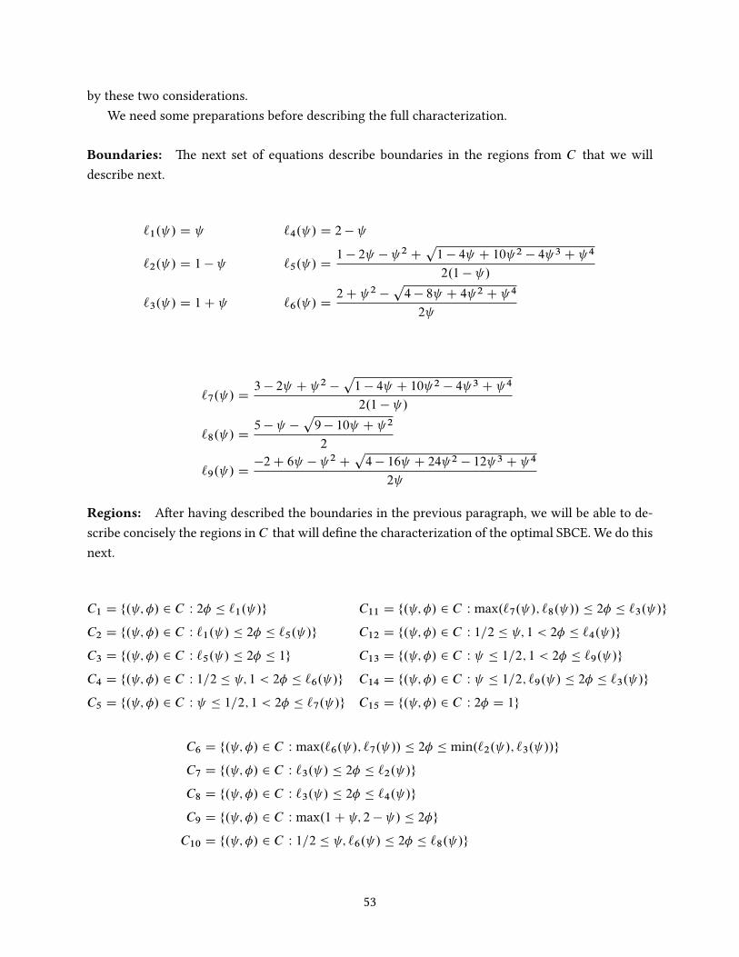
by these two considerations.We need some preparations before describing the full characterization.

Boundaries: The next set of equations describe boundaries in the regions from C that we willdescribe next.

`1. / D `4. / D 2 �

`2. / D 1 � `5. / D1 � 2 � 2 C

p1 � 4 C 10 2 � 4 3 C 4

2.1 � /

`3. / D 1C `6. / D2C 2 �

p4 � 8 C 4 2 C 4

2

`7. / D3 � 2 C 2 �

p1 � 4 C 10 2 � 4 3 C 4

2.1 � /

`8. / D5 � �

p9 � 10 C 2

2

`9. / D�2C 6 � 2 C

p4 � 16 C 24 2 � 12 3 C 4

2

Regions: After having described the boundaries in the previous paragraph, we will be able to de-scribe concisely the regions in C that will define the characterization of the optimal SBCE. We do thisnext.

C1 D f. ; �/ 2 C W 2� � `1. /g C11 D f. ; �/ 2 C W max.`7. /; `8. // � 2� � `3. /g

C2 D f. ; �/ 2 C W `1. / � 2� � `5. /g C12 D f. ; �/ 2 C W 1=2 � ; 1 < 2� � `4. /g

C3 D f. ; �/ 2 C W `5. / � 2� � 1g C13 D f. ; �/ 2 C W � 1=2; 1 < 2� � `9. /g

C4 D f. ; �/ 2 C W 1=2 � ; 1 < 2� � `6. /g C14 D f. ; �/ 2 C W � 1=2; `9. / � 2� � `3. /g

C5 D f. ; �/ 2 C W � 1=2; 1 < 2� � `7. /g C15 D f. ; �/ 2 C W 2� D 1g

C6 D f. ; �/ 2 C W max.`6. /; `7. // � 2� � min.`2. /; `3. //gC7 D f. ; �/ 2 C W `3. / � 2� � `2. /g

C8 D f. ; �/ 2 C W `3. / � 2� � `4. /g

C9 D f. ; �/ 2 C W max.1C ; 2 � / � 2�g

C10 D f. ; �/ 2 C W 1=2 � ; `6. / � 2� � `8. /g

53

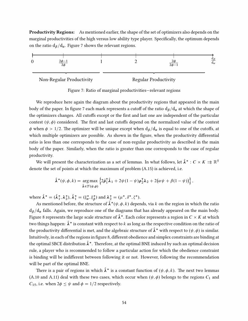
Productivity Regions: Asmentioned earlier, the shape of the set of optimizers also depends on themarginal productivities of the high versus low ability type player. Specifically, the optimum dependson the ratio dˇ=d˛ . Figure 7 shows the relevant regions.

dˇ

d˛0 2��1

2�1 2 2�

2��1

Non-Regular Productivity Regular Productivity

Figure 7: Ratio of marginal productivities—relevant regions

We reproduce here again the diagram about the productivity regions that appeared in the mainbody of the paper. In figure 7 each mark represents a cutoff of the ratio dˇ=d˛ at which the shape ofthe optimizers changes. All cutoffs except or the first and last one are independent of the particularcontest . ; �/ considered. The first and last cutoffs depend on the normalized value of the contest� when � > 1=2:The optimizer will be unique except when dˇ=d˛ is equal to one of the cutoffs, atwhich multiple optimizers are possible. As shown in the figure, when the productivity differentialratio is less than one corresponds to the case of non-regular productivity as described in the mainbody of the paper. Similarly, when the ratio is greater than one corresponds to the case of regularproductivity.

We will present the characterization as a set of lemmas. In what follows, let O�� W C � K � R5

denote the set of points at which the maximum of problem (A.15) is achieved, i.e.

O��. ; �; k/ D argmaxO�2� . ;�/

n2 O�

|1

O�1 C 2 .1 � /�|2�2 C 2

�˛ C ˇ.1 � /

�o;

where O�� D . O��1;�

�2/, O��

1 D .��˛ ; �

�ˇ/ and ��

2 D .��; ı�; ��/.As mentioned before, the structure of O��. ; �; k/ depends, via k on the region in which the ratio

dˇ=d˛ falls. Again, we reproduce one of the diagrams that has already appeared on the main body.Figure 8 represents the large scale structure of O��: Each color represents a region in C �K at whichtwo things happen: O�� is constant with respect to k as long as the respective condition on the ratio ofthe productivity differential is met, and the algebraic structure of O�� with respect to . ; �/ is similar.Intuitively, in each of the regions in figure 8, different obedience and simplex constraints are binding atthe optimal SBCE distribution O��. Therefore, at the optimal BNE induced by such an optimal decisionrule, a player who is recommended to follow a particular action for which the obedience constraintis binding will be indifferent between following it or not. However, following the recommendationwill be part of the optimal BNE.

There is a pair of regions in which O�� is a constant function of . ; �; k/. The next two lemmas(A.10 and A.11) deal with these two cases, which occur when . ; �/ belongs to the regions C1 andC15, i.e. when 2� � and � D 1=2 respectively.

54

1=2 1

1=2

1

C1

C2 [ C3

C12C13 [ C14

C7C8

C9

�

(a) .2� � 1/=.2�/ < dˇ=d˛ < 1

1=2 1

1=2

1

C1

C2 [ C3

C12C13

C7C8

C9

C14

�

(b) .2� � 1/=.2�/ > dˇ=d˛ > 0

1=2 1

1=2

1

C1C2

C3

C4C5

C6

C7C8

C9

�

(c) 1 < dˇ=d˛ < 2

1=2 1

1=2

1

C1C2

C3

C4C5

C8 [ C9

C10

C11

�

(d) 2 < dˇ=d˛ < .2�/=.2� � 1/

1=2 1

1=2

1

C1C2

C3

C5

C8 [ C9

C4 [ C10

C11

�

(e) .2�/=.2� � 1/ < dˇ=d˛

Figure 8: Structure of O��. ; �; k/

55

Lemma A.10. For all . ; �; k/ 2 C1 �K, O��. ; �; k/ is constant and is given by

O��1 D .1; 1/; ��

2 D .1; 0; 0/:

Furthermore, O�� gives an optimal value of

NV . ; �; k/ D 2� .d˛ C ˛/C .1 � /.dˇ C ˇ/

�D 2

� k.˛/˛ C .1 � /k.ˇ/ˇ

�Proof. The optimality of O��

1 D .1; 1/ follows from lemma A.6 since � � 1=2 in the region C1. Forthe same reason, we can apply corollary A.7 to find the optimal value of ��

2 by solving the problemmax

˚�

|2�2

subject to �2 2 O� . ; �/. Since O� . ; �/ includes the non-negativity constraints and

simplex constraint for �2 D .�; ı; �/ and �|2�2 D �.d˛ C dˇ / C ıd˛ C �dˇ , it follows that the

objective is a weighted sum with weights given by �2 and in which the largest term is d˛Cdˇ . Thus,it is sufficient to show that ��

2 2 O� . ; �/:The point ��2 satisfies the non-negativity conditions so we

need to show that O2�

�2 � O� � O

1O��1 :The last expression is equivalent to0BBBBBBBBBBB@

.1 � /�

� .1 � �/

�.1 � /.1 � �/

�

0

0

1

1CCCCCCCCCCCA�

0BBBBBBBBBBB@

�12

� ��

.1 � /�12

� ��

�.1 � /.1 � �/

�

0

0

1

1CCCCCCCCCCCAFrom the last expression we can see that the inequalities from rows three to seven are trivially satis-fied. From the first row after some algebraic manipulations we get that 2� � : From the second rowwe get that 2� � 1C : Since the first one implies the second one for all . ; �/ 2 C we get that theexpression in the previous display is equivalent to 2� � . Noticing that this conditions is preciselythe one that defines the boundary of region C1, we have that ��

2 is feasible if and only if . ; �/ 2 C1:

Finally, substituting the optimal values O��1 and ��

2 into the objective A.15 and simplifying termsyields the following expression for the value of the information design problem:

NV D 2 O�|1

O��1 C 2 .1 � /�

|2��

2 C 2�˛ C ˇ.1 � /

�D 2

� .d˛ C ˛/C .1 � /.dˇ C ˇ/

�D 2

� k.˛/˛ C .1 � /k.ˇ/ˇ

�:

�

Lemma A.11. If . ; �/ 2 C15, i.e. . ; �/ D .0; 1/ � f1=2g and for all k 2 K, we have that O��. ; �; k/

is constant and is given byO��1 D .1; 1/; ��

2 D .1=4; 1=4; 1=4/:

56

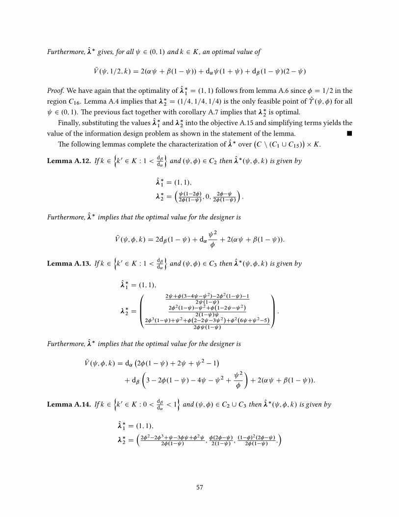
Furthermore, O�� gives, for all 2 .0; 1/ and k 2 K, an optimal value of

NV . ; 1=2; k/ D 2.˛ C ˇ.1 � //C d˛ .1C /C dˇ .1 � /.2 � /

Proof. We have again that the optimality of O��1 D .1; 1/ follows from lemma A.6 since � D 1=2 in the

region C16. Lemma A.4 implies that ��2 D .1=4; 1=4; 1=4/ is the only feasible point of O� . ; �/ for all

2 .0; 1/. The previous fact together with corollary A.7 implies that ��2 is optimal.

Finally, substituting the values O��1 and ��

2 into the objective A.15 and simplifying terms yields thevalue of the information design problem as shown in the statement of the lemma. �

The following lemmas complete the characterization of O�� over�C n .C1 [ C15/

��K:

Lemma A.12. If k 2

nk0 2 K W 1 <

dˇ

d˛

oand . ; �/ 2 C2 then O��. ; �; k/ is given by

O��1 D .1; 1/;

��2 D

� .1�2�/2�.1� /

; 0; 2�� 2�.1� /

�:

Furthermore, O�� implies that the optimal value for the designer is

NV . ; �; k/ D 2dˇ .1 � /C d˛ 2

�C 2.˛ C ˇ.1 � //:

Lemma A.13. If k 2

nk0 2 K W 1 <

dˇ

d˛

oand . ; �/ 2 C3 then O��. ; �; k/ is given by

O��1 D .1; 1/;

��2 D

0BB@2 C�.3�4 � 2/�2�2.1� /�1

2 .1� /2�2.1� /� 2C�.1�2 � 2/

2.1� / 2�3.1� /C 2C�.2�2 �3 2/C�2.6 C 2�5/

2� .1� /

1CCA :Furthermore, O�� implies that the optimal value for the designer is

NV . ; �; k/ D d˛�2�.1 � /C 2 C 2 � 1

�C dˇ

�3 � 2�.1 � / � 4 � 2 C

2

�

�C 2.˛ C ˇ.1 � //:

Lemma A.14. If k 2

nk0 2 K W 0 <

dˇ

d˛< 1

oand . ; �/ 2 C2 [ C3 then O��. ; �; k/ is given by

O��1 D .1; 1/;

��2 D

�2�2�2�3C �3� C�2

2�.1� /; �.2�� /2.1� /

; .1��/2.2�� /2�.1� /

:�

57

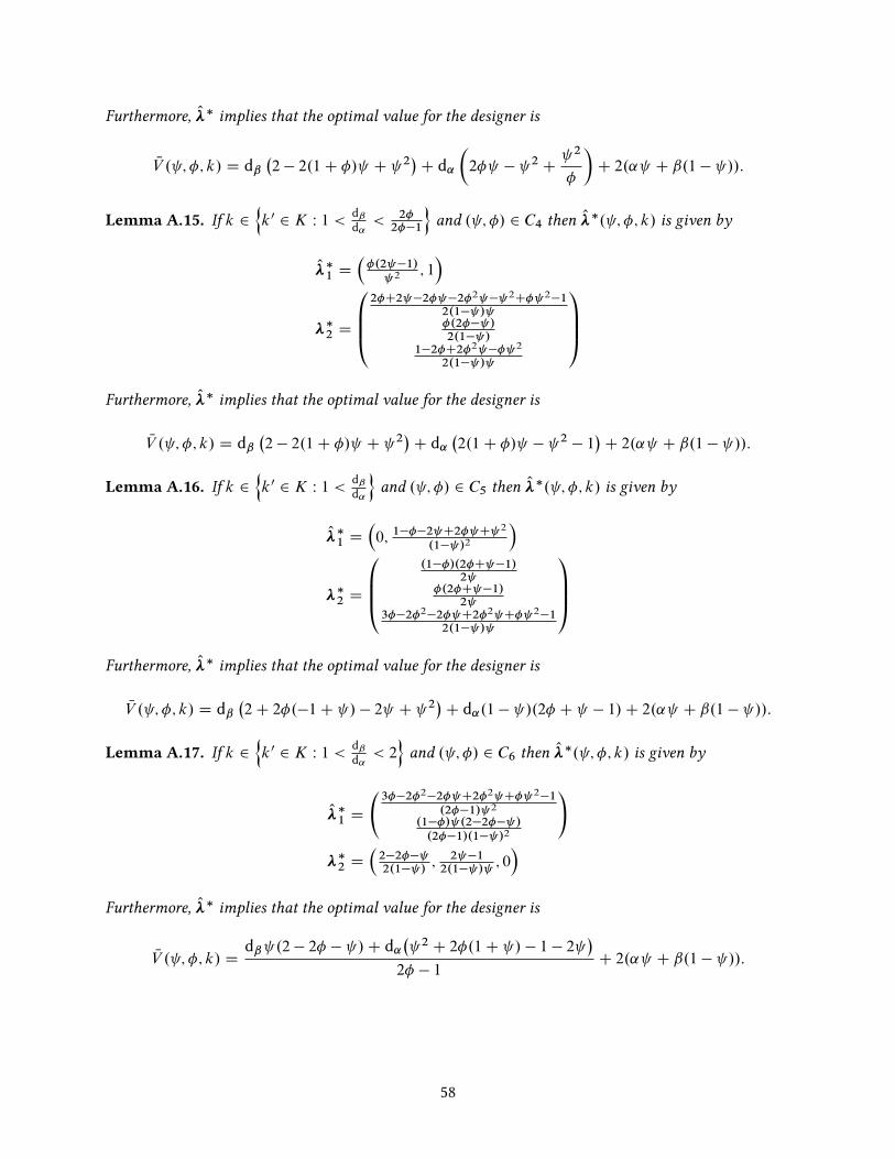
Furthermore, O�� implies that the optimal value for the designer is

NV . ; �; k/ D dˇ�2 � 2.1C �/ C 2

�C d˛

�2� � 2 C

2

�

�C 2.˛ C ˇ.1 � //:

Lemma A.15. If k 2

nk0 2 K W 1 <

dˇ

d˛< 2�2��1

oand . ; �/ 2 C4 then O��. ; �; k/ is given by

O��1 D

��.2 �1/

2 ; 1�

��2 D

0BB@2�C2 �2� �2�2 � 2C� 2�1

2.1� / �.2�� /2.1� /

1�2�C2�2 �� 2

2.1� /

1CCAFurthermore, O�� implies that the optimal value for the designer is

NV . ; �; k/ D dˇ�2 � 2.1C �/ C 2

�C d˛

�2.1C �/ � 2 � 1

�C 2.˛ C ˇ.1 � //:

Lemma A.16. If k 2

nk0 2 K W 1 <

dˇ

d˛

oand . ; �/ 2 C5 then O��. ; �; k/ is given by

O��1 D

�0; 1���2 C2� C 2

.1� /2

���2 D

[email protected]��/.2�C �1/

2 �.2�C �1/

2 3��2�2�2� C2�2 C� 2�1

2.1� /

1CCAFurthermore, O�� implies that the optimal value for the designer is

NV . ; �; k/ D dˇ�2C 2�.�1C / � 2 C 2

�C d˛.1 � /.2� C � 1/C 2.˛ C ˇ.1 � //:

Lemma A.17. If k 2

nk0 2 K W 1 <

dˇ

d˛< 2

oand . ; �/ 2 C6 then O��. ; �; k/ is given by

O��1 D

3��2�2�2� C2�2 C� 2�1

.2��1/ 2

.1��/ .2�2�� /

.2��1/.1� /2

!��2 D

�2�2�� 2.1� /

; 2 �12.1� /

; 0�

Furthermore, O�� implies that the optimal value for the designer is

NV . ; �; k/ Ddˇ .2 � 2� � /C d˛

� 2 C 2�.1C / � 1 � 2

�2� � 1

C 2.˛ C ˇ.1 � //:

58

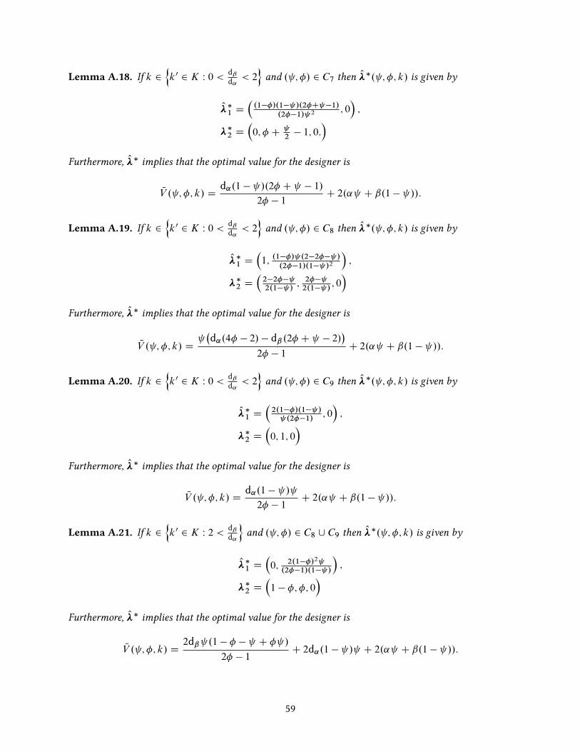
Lemma A.18. If k 2

nk0 2 K W 0 <

dˇ

d˛< 2

oand . ; �/ 2 C7 then O��. ; �; k/ is given by

O��1 D

�.1��/.1� /.2�C �1/

.2��1/ 2 ; 0�;

��2 D

�0; � C

2

� 1; 0:�

Furthermore, O�� implies that the optimal value for the designer is

NV . ; �; k/ Dd˛.1 � /.2� C � 1/

2� � 1C 2.˛ C ˇ.1 � //:

Lemma A.19. If k 2

nk0 2 K W 0 <

dˇ

d˛< 2

oand . ; �/ 2 C8 then O��. ; �; k/ is given by

O��1 D

�1; .1��/ .2�2�� /

.2��1/.1� /2

�;

��2 D

�2�2�� 2.1� /

; 2�� 2.1� /

; 0�

Furthermore, O�� implies that the optimal value for the designer is

NV . ; �; k/ D �d˛.4� � 2/ � dˇ .2� C � 2/

�2� � 1

C 2.˛ C ˇ.1 � //:

Lemma A.20. If k 2

nk0 2 K W 0 <

dˇ

d˛< 2

oand . ; �/ 2 C9 then O��. ; �; k/ is given by

O��1 D

�2.1��/.1� / .2��1/

; 0�;

��2 D

�0; 1; 0

�Furthermore, O�� implies that the optimal value for the designer is

NV . ; �; k/ Dd˛.1 � /

2� � 1C 2.˛ C ˇ.1 � //:

Lemma A.21. If k 2

nk0 2 K W 2 <

dˇ

d˛

oand . ; �/ 2 C8 [ C9 then O��. ; �; k/ is given by

O��1 D

�0; 2.1��/2 .2��1/.1� /

�;

��2 D

�1 � �; �; 0

�Furthermore, O�� implies that the optimal value for the designer is

NV . ; �; k/ D2dˇ .1 � � � C � /

2� � 1C 2d˛.1 � / C 2.˛ C ˇ.1 � //:

59

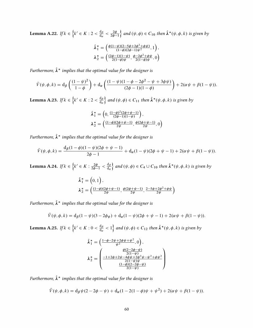
Lemma A.22. If k 2

nk0 2 K W 2 <

dˇ

d˛< 2�2��1

oand . ; �/ 2 C10 then O��. ; �; k/ is given by

O��1 D

��.1� /.2�5�C2�2C� /

.1��/.2��1/ 2 ; 1�;

��2 D

�.2��1/.1� /2.1��/

; ��2�2C� 2.1��/

; 0�

Furthermore, O�� implies that the optimal value for the designer is

NV . ; �; k/ D dˇ�.1 � /2

1 � �

�C d˛

�.1 � /.1 � � � 2�2 � C 3� /

.2� � 1/.1 � �/

�C 2.˛ C ˇ.1 � //:

Lemma A.23. If k 2

nk0 2 K W 2 <

dˇ

d˛

oand . ; �/ 2 C11 then O��. ; �; k/ is given by

O��1 D

�0; .1��/2.2�C �1/

.2��1/.1� /

�;

��2 D

�.1��/.2�C �1/

2 ; �.2�C �1/

2 ; 0�

Furthermore, O�� implies that the optimal value for the designer is

NV . ; �; k/ Ddˇ .1 � �/.1 � /.2� C � 1/

2� � 1C d˛.1 � /.2� C � 1/C 2.˛ C ˇ.1 � //:

Lemma A.24. If k 2

nk0 2 K W

2�2��1

<dˇ

d˛

oand . ; �/ 2 C4 [ C10 then O��. ; �; k/ is given by

O��1 D

�0; 1

�;

��2 D

�.1��/.2�C �1/

2 ; �.2�C �1/

2 ; 2�5�C2�2C�

2

�Furthermore, O�� implies that the optimal value for the designer is

NV . ; �; k/ D dˇ .1 � /.3 � 2� /C d˛.1 � /.2� C � 1/C 2.˛ C ˇ.1 � //:

Lemma A.25. If k 2

nk0 2 K W 0 <

dˇ

d˛< 1

oand . ; �/ 2 C12 then O��. ; �; k/ is given by

O��1 D

�1���2 C2� C 2

2 ; 0�;

��2 D

0BB@�.2�2�� /2.1� /

�1C2�C2 �4� C2�2 � 2C� 2

2.1� / .1��/.2�2�� /

2.1� /

1CCAFurthermore, O�� implies that the optimal value for the designer is

NV . ; �; k/ D dˇ .2 � 2� � /C d˛.1 � 2.1 � �/ C 2/C 2.˛ C ˇ.1 � //:

60

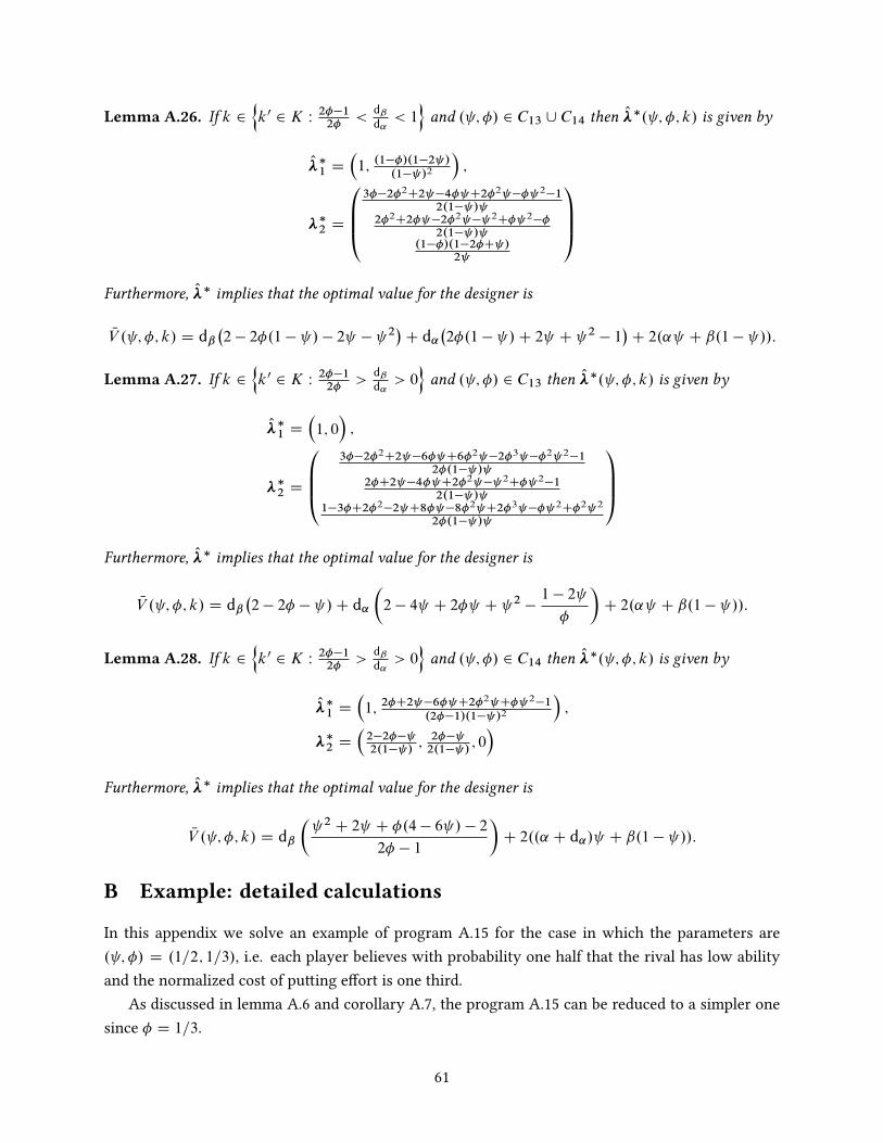
Lemma A.26. If k 2

nk0 2 K W

2��12�

<dˇ

d˛< 1

oand . ; �/ 2 C13 [ C14 then O��. ; �; k/ is given by

O��1 D

�1; .1��/.1�2 /

.1� /2

�;

��2 D

0BB@3��2�2C2 �4� C2�2 �� 2�1

2.1� / 2�2C2� �2�2 � 2C� 2��

2.1� / .1��/.1�2�C /

2

1CCAFurthermore, O�� implies that the optimal value for the designer is

NV . ; �; k/ D dˇ�2 � 2�.1 � / � 2 � 2

�C d˛

�2�.1 � /C 2 C 2 � 1

�C 2.˛ C ˇ.1 � //:

Lemma A.27. If k 2

nk0 2 K W

2��12�

>dˇ

d˛> 0

oand . ; �/ 2 C13 then O��. ; �; k/ is given by

O��1 D

�1; 0

�;

��2 D

0BB@3��2�2C2 �6� C6�2 �2�3 ��2 2�1

2�.1� / 2�C2 �4� C2�2 � 2C� 2�1

2.1� / 1�3�C2�2�2 C8� �8�2 C2�3 �� 2C�2 2

2�.1� /

1CCAFurthermore, O�� implies that the optimal value for the designer is

NV . ; �; k/ D dˇ�2 � 2� � /C d˛

�2 � 4 C 2� C 2 �

1 � 2

�

�C 2.˛ C ˇ.1 � //:

Lemma A.28. If k 2

nk0 2 K W

2��12�

>dˇ

d˛> 0

oand . ; �/ 2 C14 then O��. ; �; k/ is given by

O��1 D

�1; 2�C2 �6� C2�2 C� 2�1

.2��1/.1� /2

�;

��2 D

�2�2�� 2.1� /

; 2�� 2.1� /

; 0�

Furthermore, O�� implies that the optimal value for the designer is

NV . ; �; k/ D dˇ� 2 C 2 C �.4 � 6 / � 2

2� � 1

�C 2..˛ C d˛/ C ˇ.1 � //:

B Example: detailed calculations

In this appendix we solve an example of program A.15 for the case in which the parameters are. ; �/ D .1=2; 1=3/, i.e. each player believes with probability one half that the rival has low abilityand the normalized cost of putting effort is one third.

As discussed in lemma A.6 and corollary A.7, the program A.15 can be reduced to a simpler onesince � D 1=3.

61

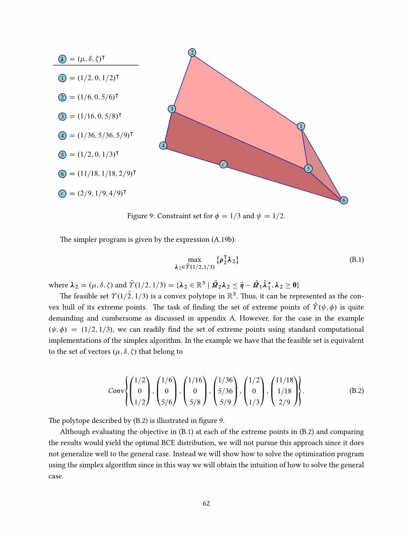
� D .�; ı; �/|

1 D .1=2; 0; 1=2/|

2 D .1=6; 0; 5=6/|

3 D .1=16; 0; 5=8/|

4 D .1=36; 5=36; 5=9/|

5 D .1=2; 0; 1=3/|

6 D .11=18; 1=18; 2=9/|

c D .2=9; 1=9; 4=9/|

1

2

3

4

5

6

c

Figure 9: Constraint set for � D 1=3 and D 1=2.

The simpler program is given by the expression (A.19b):

max�22 O� .1=2;1=3/

˚�

|2�2

(B.1)

where �2 D .�; ı; �/ and O� .1=2; 1=3/ D f�2 2 R3 j O2�2 � O� � O

1O��1;�2 � 0g

The feasible set O� .1=2; 1=3/ is a convex polytope in R3: Thus, it can be represented as the con-vex hull of its extreme points. The task of finding the set of extreme points of O� . ; �/ is quitedemanding and cumbersome as discussed in appendix A. However, for the case in the example. ; �/ D .1=2; 1=3/, we can readily find the set of extreme points using standard computationalimplementations of the simplex algorithm. In the example we have that the feasible set is equivalentto the set of vectors .�; ı; �/ that belong to

Conv

�0B@1=201=2

1CA ;0B@1=605=6

1CA ;0B@1=1605=8

1CA ;0B@1=365=36

5=9

1CA ;0B@1=201=3

1CA ;0B@11=181=18

2=9

1CA�

: (B.2)

The polytope described by (B.2) is illustrated in figure 9.Although evaluating the objective in (B.1) at each of the extreme points in (B.2) and comparing

the results would yield the optimal BCE distribution, we will not pursue this approach since it doesnot generalize well to the general case. Instead we will show how to solve the optimization programusing the simplex algorithm since in this way we will obtain the intuition of how to solve the generalcase.

62

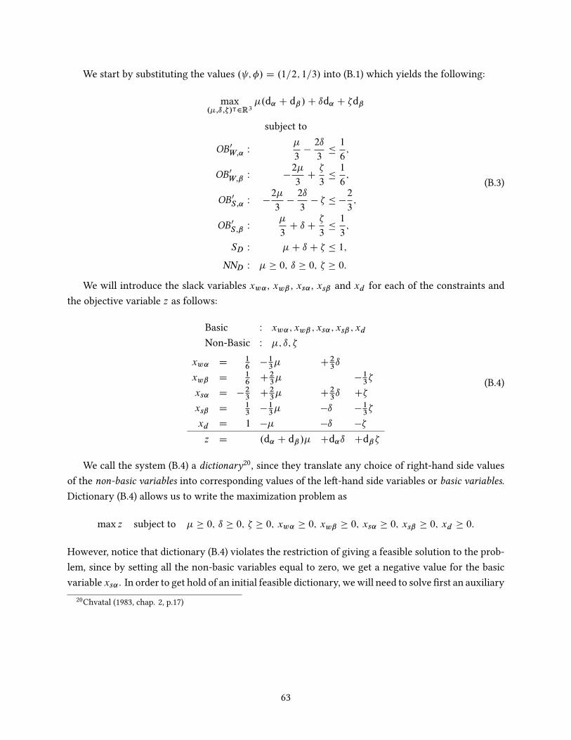
We start by substituting the values . ; �/ D .1=2; 1=3/ into (B.1) which yields the following:

max.�;ı;�/|2R3

�.d˛ C dˇ /C ıd˛ C �dˇ

subject to

OB 0W;˛ W

�

3�2ı

3�1

6;

OB 0W;ˇ W �

2�

3C�

3�1

6;

OB 0S;˛ W �

2�

3�2ı

3� � � �

2

3;

OB 0S;ˇ W

�

3C ı C

�

3�1

3;

SD W �C ı C � � 1;

NND W � � 0; ı � 0; � � 0:

(B.3)

We will introduce the slack variables xw˛ , xwˇ , xs˛ , xsˇ and xd for each of the constraints andthe objective variable z as follows:

Basic W xw˛; xwˇ ; xs˛; xsˇ ; xd

Non-Basic W �; ı; �

xw˛ D16

�13� C

23ı

xwˇ D16

C23� �

13�

xs˛ D �23

C23� C

23ı C�

xsˇ D13

�13� �ı �

13�

xd D 1 �� �ı ��

z D .d˛ C dˇ /� Cd˛ı Cdˇ �

(B.4)

We call the system (B.4) a dictionary20, since they translate any choice of right-hand side valuesof the non-basic variables into corresponding values of the left-hand side variables or basic variables.Dictionary (B.4) allows us to write the maximization problem as

max z subject to � � 0; ı � 0; � � 0; xw˛ � 0; xwˇ � 0; xs˛ � 0; xsˇ � 0; xd � 0:

However, notice that dictionary (B.4) violates the restriction of giving a feasible solution to the prob-lem, since by setting all the non-basic variables equal to zero, we get a negative value for the basicvariable xs˛ . In order to get hold of an initial feasible dictionary, wewill need to solve first an auxiliary

20Chvatal (1983, chap. 2, p.17)

63

problem:min

.�;ı;�;x0/|2R4x0

subject to�

3�2ı

3� x0 �

1

6;

�2�

3C�

3� x0 �

1

6;

�2�

3�2ı

3� � � x0 � �

2

3;

�

3C ı C

�

3� x0 �

1

3;

�C ı C � � x0 � 1;

� � 0; ı � 0; � � 0;

which is actually equivalent to maximizing �x0. Again, writing down the slack variables xw˛ , xwˇ ,xs˛ , xsˇ and xd and the objective function w D �x0 we obtain the dictionary:

Basic W xw˛; xwˇ ; xs˛; xsˇ ; xd

Non-Basic W �; ı; �; x0

xw˛ D16

�13� C

23ı Cx0

xwˇ D16

C23� �

13� Cx0

xs˛ D �23

C23� C

23ı C� Cx0

xsˇ D13

�13� �ı �

13� Cx0

xd D 1 �� �ı �� Cx0

w D �x0

(B.5)

Let s • t denote the replacement-pivoting operation in which variable s enters the basis andvariable t leaves it. Dictionary (B.5) is also infeasible but it can be transformed into a feasible one bythe operation x0 • xs˛ , which yields the dictionary:

Basic W x0; xw˛; xwˇ ; xsˇ ; xd

Non-Basic W �; ı; �; xs˛

x0 D23

�23� �

23ı �� Cxs˛

xw˛ D56

�� �� Cxs˛

xwˇ D56

�23ı �

43� Cxs˛

xsˇ D 1 �� �53ı �

43� Cxs˛

xd D53

�53� �

53ı �2� Cxs˛

w D �23

C23� C

23ı C� �xs˛

(B.6)

The next dictionary is obtained by the operation � • xwˇ , which yields:

64

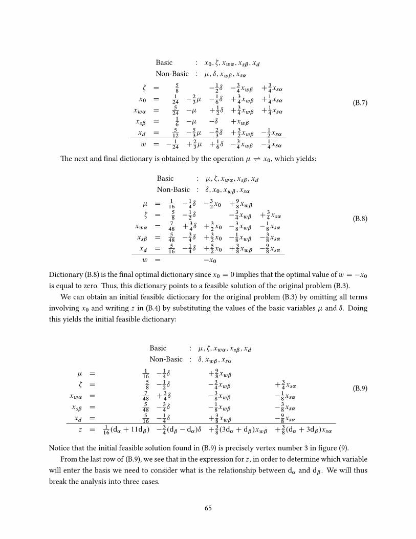
Basic W x0; �; xw˛; xsˇ ; xd

Non-Basic W �; ı; xwˇ ; xs˛

� D58

�12ı �

34xwˇ C

34xs˛

x0 D124

�23� �

16ı C

34xwˇ C

14xs˛

xw˛ D524

�� C12ı C

34xwˇ C

14xs˛

xsˇ D16

�� �ı Cxwˇ

xd D512

�53� �

23ı C

32xwˇ �

12xs˛

w D �124

C23� C

16ı �

34xwˇ �

14xs˛

(B.7)

The next and final dictionary is obtained by the operation � • x0, which yields:

Basic W �; �; xw˛; xsˇ ; xd

Non-Basic W ı; x0; xwˇ ; xs˛

� D116

�14ı �

32x0 C

98xwˇ

� D58

�12ı �

34xwˇ C

34xs˛

xw˛ D748

C34ı C

32x0 �

38xwˇ �

18xs˛

xsˇ D548

�34ı C

32x0 �

18xwˇ �

38xs˛

xd D516

�14ı C

52x0 C

38xwˇ �

98xs˛

w D �x0

(B.8)

Dictionary (B.8) is the final optimal dictionary since x0 D 0 implies that the optimal value ofw D �x0

is equal to zero. Thus, this dictionary points to a feasible solution of the original problem (B.3).We can obtain an initial feasible dictionary for the original problem (B.3) by omitting all terms

involving x0 and writing z in (B.4) by substituting the values of the basic variables � and ı. Doingthis yields the initial feasible dictionary:

Basic W �; �; xw˛; xsˇ ; xd

Non-Basic W ı; xwˇ ; xs˛

� D116

�14ı C

98xwˇ

� D58

�12ı �

34xwˇ C

34xs˛

xw˛ D748

C34ı �

38xwˇ �

18xs˛

xsˇ D548

�34ı �

18xwˇ �

38xs˛

xd D516

�14ı C

38xwˇ �

98xs˛

z D116.d˛ C 11dˇ / �

34.dˇ � d˛/ı C

38.3d˛ C dˇ /xwˇ C

38.d˛ C 3dˇ /xs˛

(B.9)

Notice that the initial feasible solution found in (B.9) is precisely vertex number 3 in figure (9).From the last row of (B.9), we see that in the expression for z, in order to determine which variable

will enter the basis we need to consider what is the relationship between d˛ and dˇ . We will thusbreak the analysis into three cases.

65

Case 1: dˇ > d˛. In this case the coefficient on ı in the last row of (B.9) is negative and thecoefficient on xwˇ is positive and strictly smaller than the coefficient on xs˛ . The next dictionary isobtained by the operation xs˛ • xsˇ which yields the dictionary:

Basic W �; �; xw˛; xs˛; xd

Non-Basic W ı; xwˇ ; xsˇ

� D16

�ı Cxwˇ �xsˇ

� D56

�2ı �xwˇ �2xsˇ

xw˛ D19

Cı �13xwˇ C

13xsˇ

xs˛ D518

�2ı �13xwˇ �

83xsˇ

xd D C2ı C3xsˇ

z D16d˛ C dˇ �3dˇ ı Cd˛xwˇ �.3dˇ C d˛/xsˇ

(B.10)

The next and final dictionary is obtained by the operation xwˇ • xw˛ which yields:

Basic W �; �; xwˇ ; xs˛; xd

Non-Basic W ı; xw˛; xsˇ

� D12

C2ı �3xw˛

� D12

�5ı C3xw˛ �3xsˇ

xwˇ D13

C3ı �3xw˛ Cxsˇ

xs˛ D16

�3ı Cxw˛ �3xsˇ

xd D C2ı C3xsˇ

z D12d˛ C dˇ �3.dˇ � d˛/ı �3d˛xw˛ �3dˇxsˇ

(B.11)

The optimal solution implies that ı D xw˛ D xwˇ D 0. Thus we have that

.�; ı; �; xw˛; xwˇ ; xs˛; xsˇ ; xd /|

D .1=2; 0; 1=2; 0; 1=3; 1=6; 0; 0/|: (B.12)

Case 2: dˇ < d˛. In this case all the coefficients in the last row of (B.9) are positive. However, thecoefficient on xwˇ is the largest of three. The next dictionary is obtained by performing the operationxwˇ • xw˛ which yields the dictionary

Basic W �; �; xwˇ ; xsˇ ; xd

Non-Basic W ı; xw˛; xs˛

� D12

C2ı �3xw˛

� D13

�2ı C2xw˛ Cxs˛

xwˇ D718

C2ı �83xw˛ �

13xs˛

xsˇ D118

�ı C13xw˛ �

13xs˛

xd D16

�ı Cxw˛ �xs˛

z D12d˛ C

56dˇ C3d˛ı �.3d˛ C dˇ /xw˛ Cdˇxs˛

(B.13)

66

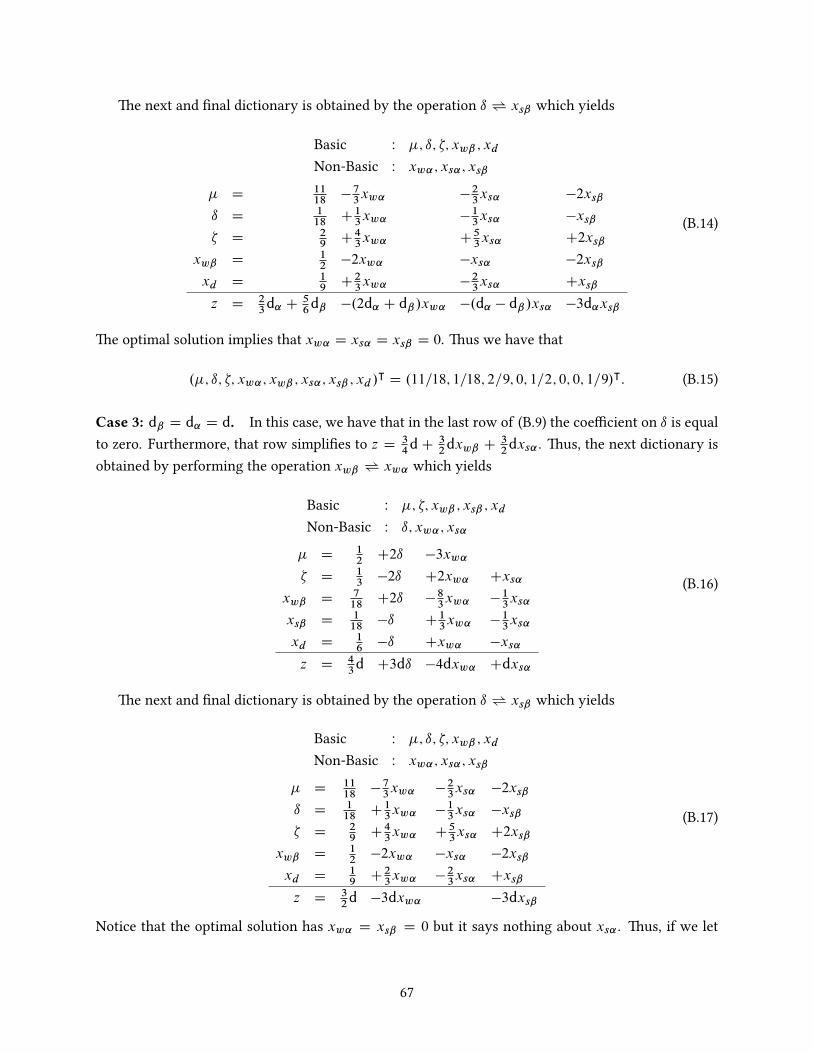
The next and final dictionary is obtained by the operation ı • xsˇ which yields

Basic W �; ı; �; xwˇ ; xd

Non-Basic W xw˛; xs˛; xsˇ

� D1118

�73xw˛ �

23xs˛ �2xsˇ

ı D118

C13xw˛ �

13xs˛ �xsˇ

� D29

C43xw˛ C

53xs˛ C2xsˇ

xwˇ D12

�2xw˛ �xs˛ �2xsˇ

xd D19

C23xw˛ �

23xs˛ Cxsˇ

z D23d˛ C

56dˇ �.2d˛ C dˇ /xw˛ �.d˛ � dˇ /xs˛ �3d˛xsˇ

(B.14)

The optimal solution implies that xw˛ D xs˛ D xsˇ D 0. Thus we have that

.�; ı; �; xw˛; xwˇ ; xs˛; xsˇ ; xd /|

D .11=18; 1=18; 2=9; 0; 1=2; 0; 0; 1=9/|: (B.15)

Case 3: dˇ D d˛ D d. In this case, we have that in the last row of (B.9) the coefficient on ı is equalto zero. Furthermore, that row simplifies to z D

34d C

32dxwˇ C

32dxs˛ . Thus, the next dictionary is

obtained by performing the operation xwˇ • xw˛ which yields

Basic W �; �; xwˇ ; xsˇ ; xd

Non-Basic W ı; xw˛; xs˛

� D12

C2ı �3xw˛

� D13

�2ı C2xw˛ Cxs˛

xwˇ D718

C2ı �83xw˛ �

13xs˛

xsˇ D118

�ı C13xw˛ �

13xs˛

xd D16

�ı Cxw˛ �xs˛

z D43d C3dı �4dxw˛ Cdxs˛

(B.16)

The next and final dictionary is obtained by the operation ı • xsˇ which yields

Basic W �; ı; �; xwˇ ; xd

Non-Basic W xw˛; xs˛; xsˇ

� D1118

�73xw˛ �

23xs˛ �2xsˇ

ı D118

C13xw˛ �

13xs˛ �xsˇ

� D29

C43xw˛ C

53xs˛ C2xsˇ

xwˇ D12

�2xw˛ �xs˛ �2xsˇ

xd D19

C23xw˛ �

23xs˛ Cxsˇ

z D32d �3dxw˛ �3dxsˇ

(B.17)

Notice that the optimal solution has xw˛ D xsˇ D 0 but it says nothing about xs˛ . Thus, if we let

67

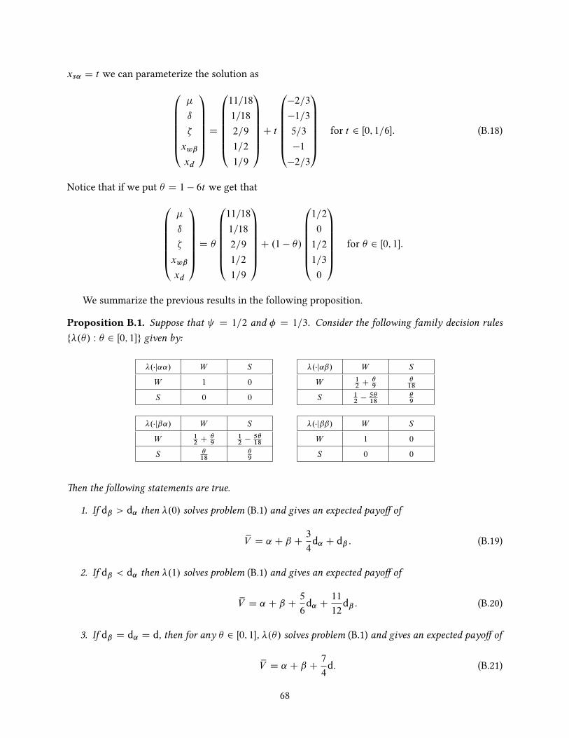
xs˛ D t we can parameterize the solution as0BBBBBB@�

ı

�

xwˇ

xd

1CCCCCCA D

0BBBBBB@11=18

1=18

2=9

1=2

1=9

1CCCCCCAC t

0BBBBBB@�2=3

�1=3

5=3

�1

�2=3

1CCCCCCA for t 2 Œ0; 1=6�. (B.18)

Notice that if we put � D 1 � 6t we get that0BBBBBB@�

ı

�

xwˇ

xd

1CCCCCCA D �

0BBBBBB@11=18

1=18

2=9

1=2

1=9

1CCCCCCAC .1 � �/

0BBBBBB@1=2

0

1=2

1=3

0

1CCCCCCA for � 2 Œ0; 1�.

We summarize the previous results in the following proposition.

Proposition B.1. Suppose that D 1=2 and � D 1=3. Consider the following family decision rulesf�.�/ W � 2 Œ0; 1�g given by:

�.�j˛˛/ W S

W 1 0

S 0 0

�.�j˛ˇ/ W S

W 12 C

�9

�18

S 12 �

5�18

�9

�.�jˇ˛/ W S

W 12 C

�9

12 �

5�18

S �18

�9

�.�jˇˇ/ W S

W 1 0

S 0 0

Then the following statements are true.

1. If dˇ > d˛ then �.0/ solves problem (B.1) and gives an expected payoff of

xV D ˛ C ˇ C3

4d˛ C dˇ : (B.19)

2. If dˇ < d˛ then �.1/ solves problem (B.1) and gives an expected payoff of

xV D ˛ C ˇ C5

6d˛ C

11

12dˇ : (B.20)

3. If dˇ D d˛ D d, then for any � 2 Œ0; 1�, �.�/ solves problem (B.1) and gives an expected payoff of

xV D ˛ C ˇ C7

4d: (B.21)

68

There are some features about the optimum characterized in B.1 that are worth remarking. In thesearch for an optimum, it is important to note that we always take that the basic variables at eachdictionary are positive. In the general case this will provide new restrictions that the parameters . ; �/need to satisfy. Also, the termination condition in the simplex algorithm requires that all coefficientsof the non-basic variables that appear in the last row of a dictionary to be negative. Notice from ourcalculations that in the last row z of the dictionary all the coefficients have to do with functions of dˇand d˛ . In particular, the determining condition is whether the ratio of these two, dˇ=d˛ is strictlygreater, strictly less or equal to one. Thus the shape of the optimum depends on how the marginalproductivities behave. Furthermore, notice that multiplicity in this case occurs when dˇ=d˛ D 1 i.e.when the marginal productivites are the same. These type of conditions arise in a similar way in thegeneral case.

References

Angeletos, G.-M. andA. Pavan (2007): “Efficient use of information and social value of information,”Econometrica, 75, 1103–1142.

Aumann, R. J. (1974): “Subjectivity and correlation in randomized strategies,” Journal of MathematicalEconomics, 1, 67–96.

——— (1987): “Correlated equilibrium as an expression of Bayesian rationality,” Econometrica, 1–18.

Aumann, R. J., M. Maschler, and R. E. Stearns (1995): Repeated games with incomplete information,MIT press.

Battigalli, P. (2018): “Game Theory, Analysis of Strategic Thinking,” Bocconi Univer-sity, URL: http://didattica.unibocconi.eu/mypage/doc.php?idDoc=29501&IdUte=48808&idr=703&Tipo=m&lingua=eng.

Benoît, J.-P. and J. Dubra (2011): “Apparent overconfidence,” Econometrica, 79, 1591–1625.

Bergemann, D. and S. Morris (2013): “Bayes correlated equilibrium and the comparison of infor-mation structures in games,” Technical Report 1822R, Cowles Foundation for Research in Economics,Yale University.

——— (2016): “Bayes correlated equilibrium and the comparison of information structures in games,”Theoretical Economics, 11, 487–522.

——— (2018): “Information Design: A Unified Perspective,” Cowles Foundation Discussion Paper No.2075R3.

Brandenburger, A. and E. Dekel (1993): “Hierarchies of beliefs and common knowledge,” Journalof Economic Theory, 59, 189–198.

69

Brocas, I. and J. D. Carrillo (2007): “Influence through ignorance,”The RAND Journal of Economics,38, 931–947.

Carroll, G. (2016): “Informationally robust trade and limits to contagion,” Journal of Economic The-ory, 166, 334–361.

Chvatal, V. (1983): Linear Programming, New York: W.H. Freeman.

Crawford, V. P. and J. Sobel (1982): “Strategic information transmission,” Econometrica: Journal ofthe Econometric Society, 1431–1451.

Denter, P., J. Morgan, and D. Sisak (2014): “’Where Ignorance is Bliss,’Tis Folly to BeWise’: Trans-parency in Contests,” Working paper.

Dubey, P. (2013): “The role of information in contests,” Economics Letters, 120, 160–163.

Eckhoff, J., P. Gruber, and J. Wills (1993): Handbook of Convex Geometry, North-Holland Amster-dam, Netherlands.

Einy, E., D. Moreno, and B. Shitovitz (2017): “The value of public information in common-valueTullock contests,” Economic Theory, 63, 925–942.

Ely, J., A. Frankel, and E. Kamenica (2015): “Suspense and surprise,” Journal of Political Economy,123, 215–260.

Epstein, G. S. and Y.Mealem (2013): “Who gains from information asymmetry?” Theory and decision,75, 305–337.

Fagin, R., J. Y. Halpern, Y. Moses, and M. Vardi (2004): Reasoning about knowledge, MIT press.

Fey, M. (2008): “Rent-seeking contests with incomplete information,” Public Choice, 135, 225–236.

Fu, Q., O. Gürtler, and J. Münster (2013): “Communication and commitment in contests,” Journalof Economic Behavior & Organization, 95, 1–19.

Fu, Q., J. Lu, and J. Zhang (2016): “Disclosure policy in Tullock contests with asymmetric stochasticentry,” Canadian Journal of Economics/Revue canadienne d’économique, 49, 52–75.

Gale, D. (1989): Theory of linear economic models, Chicago: University of Chicago Press, reprint ofthe 1960 edition published by McGraw-Hill.

Gentzkow, M. and E. Kamenica (2014): “Costly persuasion,” American Economic Review, 104, 457–62.

Gürtler, O., J. Münster, and P. Nieken (2013): “Information policy in tournaments with sabotage,”The Scandinavian Journal of Economics, 115, 932–966.

70

Harsanyi, J. C. (1967): “Games with incomplete information played by “Bayesian” players, I–III PartI. The basic model,” Management science, 14, 159–182.

——— (1968a): “Games with incomplete information played by “Bayesian” players part II. Bayesianequilibrium points,” Management Science, 14, 320–334.

——— (1968b): “Games with incomplete information played by “Bayesian” players, part III. The basicprobability distribution of the game,” Management Science, 14, 486–502.

Kamenica, E. (2018): “Bayesian persuasion and information design,” Working paper, University ofChicago.

Kamenica, E. and M. Gentzkow (2011): “Bayesian persuasion,” The American Economic Review, 101,2590–2615.

Kolotilin, A., T. Mylovanov, A. Zapechelnyuk, and M. Li (2017): “Persuasion of a privately in-formed receiver,” Econometrica, 85, 1949–1964.

Kramm, M. (2018): “Information Design in Multi-Task Contests—Whom to Inform When the Impor-tance of Tasks is Uncertain,” Working paper.

Lim, W. and A. Matros (2009): “Contests with a stochastic number of players,” Games and EconomicBehavior, 67, 584–597.

Lipnowski, E. and L.Mathevet (2018): “Disclosure to a Psychological Audience,”American EconomicJournal: Microeconomics, 10, 67–93.

Maschler, M., E. Solan, and S. Zamir (2013): Game Theory, Cambridge University Press.

Mathevet, L., J. Perego, and I. Taneva (2016): “Information Design: The Belief Hierarchy Ap-proach,” Working paper.

Mertens, J.-F. and S. Zamir (1985): “Formulation of Bayesian analysis for games with incompleteinformation,” International Journal of Game Theory, 14, 1–29.

Moldovanu, B. and A. Sela (2001): “The optimal allocation of prizes in contests,” American EconomicReview, 91, 542–558.

Morath, F. and J. Münster (2013): “Information acquisition in conflicts,” Economic Theory, 54, 99–129.

Morris, S. and H. S. Shin (2002): “Social value of public information,” American Economic review, 92,1521–1534.

Münster, J. (2009): “Repeated contests with asymmetric information,” Journal of Public EconomicTheory, 11, 89–118.

71

Myerson, R. B. (1979): “Incentive compatibility and the bargaining problem,” Econometrica, 61–73.

——— (1991): Game theory: analysis of conflict, Harvard University Press, 1st Paperback Edition, 1997.

Salomone, R., R. Vaisman, and D. P. Kroese (2016): “Estimating the Number of Vertices in Con-vex Polytopes,” in Proceedings of the International Conference on Operations Research and Statistics,Citeseer, 96–105.

Taneva, I. (2015): “Information design,” Working Paper, Department of Economics, University ofEdinburgh.

Vives, X. (1988): “Aggregation of information in large Cournot markets,” Econometrica: Journal of theEconometric Society, 851–876.

Zamir, S. (2009): “Bayesian Games: Games with Incomplete Information,” in Encyclopedia of Com-plexity and Systems Science.

Zhang, J. and J. Zhou (2016): “Information disclosure in contests: A Bayesian persuasion approach,”The Economic Journal, 126, 2197–2217.

72