The SCUBA-2 Cosmology Legacy Survey: 850 and number counts

Mon. Not. R. Astron. Soc. 000, 000–000 (0000) Printed 13 July 2016 (MN LATEX style file v2.2)

The SCUBA-2 Cosmology Legacy Survey: 850µm maps, cataloguesand number counts

J. E. Geach1?, J. S. Dunlop2, M. Halpern3, Ian Smail4, P. van der Werf5,D. M. Alexander4, O. Almaini6, I. Aretxaga7, V. Arumugam2,8, V. Asboth3, M. Banerji9,J. Beanlands10, P. N. Best2, A. W. Blain11, M. Birkinshaw12, E. L. Chapin13,S. C. Chapman14, C-C. Chen4, A. Chrysostomou15, C. Clarke16, D. L. Clements17,C. Conselice6, K. E. K. Coppin1, W. I. Cowley18, A. L. R. Danielson4, S. Eales19,A. C. Edge4, D. Farrah20, A. Gibb3, C. M. Harrison4, N. K. Hine1, D. Hughes7,R. J. Ivison2,8, M. Jarvis21,22, T. Jenness3, S. F. Jones23, A. Karim24, M. Koprowski1,K. K. Knudsen23, C. G. Lacey18, T. Mackenzie3, G. Marsden3, K. McAlpine22,R. McMahon8, R. Meijerink5,25, M. J. Michałowski3, S. J. Oliver16, M. J. Page26,J. A. Peacock2, D. Rigopoulou21,27, E. I. Robson2,28, I. Roseboom2, K. Rotermund14,Douglas Scott3, S. Serjeant29, C. Simpson30, J. M. Simpson2, D. J. B. Smith1,M. Spaans25, F. Stanley4, J. A. Stevens1, A. M. Swinbank4, T. Targett31, A. P. Thomson4,E. Valiante19, T. M. A. Webb32, C. Willott33, J. A. Zavala7, M. Zemcov34,35

1 Centre for Astrophysics Research, School of Physics, Astronomy & Mathematics, University of Hertfordshire, Hatfield, AL10 9ABOther affiliations at end

13 July 2016

ABSTRACTWe present a catalogue of nearly 3,000 submillimetre sources detected (>3.5σ) at 850µmover ∼5 deg2 surveyed as part of the James Clerk Maxwell Telescope (JCMT) SCUBA-2Cosmology Legacy Survey (S2CLS). This is the largest survey of its kind at 850µm, probinga meaningful cosmic volume at the peak of star formation activity and increasing the sam-ple size of submillimetre galaxies selected at 850µm by an order of magnitude. We describethe wide 850µm survey component of S2CLS, which covers the key extragalactic surveyfields: UKIDSS-UDS, COSMOS, Akari-NEP, Extended Groth Strip, Lockman Hole North,SSA22 and GOODS-North. The average 1σ depth of S2CLS is 1.2 mJy beam−1, approach-ing the SCUBA-2 850µm confusion limit, which we determine to be σc ≈ 0.8mJy beam−1.We measure the single dish 850µm number counts to unprecedented accuracy, reducing thePoisson errors on the differential counts to approximately 4% at S850 ≈ 3mJy. With severalindependent fields, we investigate field-to-field variance, finding that the number counts on0.5–1 scales are generally within 50% of the S2CLS mean for S850 > 3mJy, with scat-ter consistent with the Poisson and estimated cosmic variance uncertainties, although thereis a marginal (2σ) density enhancement in the GOODS-North field. The observed numbercounts are in reasonable agreement with recent phenomenological and semi-analytic models,although robustly determining the shape of the faint end slope (S850 < 3mJy) remains a keytest. Finally, the large solid angle of S2CLS allows us to measure the bright-end counts: atS850 > 10mJy there are approximately ten sources per square degree, and we detect the dis-tinctive up-turn in the number counts indicative of the detection of local sources of 850µmemission, and strongly lensed high-redshift galaxies. Here we describe the data collection andreduction procedures and present calibrated maps and a catalogue of sources; these are madepublicly available.

Key words: surveys – catalogues – galaxies: high-redshift – galaxies: evolution – cosmology:observations

? E-mail: [email protected]

c© 0000 RAS

arX

iv:1

607.

0390

4v1

[as

tro-

ph.G

A]

13

Jul 2

016

2 J. E. Geach et al.

1 INTRODUCTION

Nearly a quarter of a century has passed since it was predictedthat submillimetre observations could provide important insightsinto the nature of galaxies in the early Universe beyond the reachof optical and near-infrared surveys (Blain & Longair 1993). Ifearly star-forming galaxies contained dust then ultraviolet photonsshould be reprocessed through the far-infrared (Hildebrand 1983)and redshifted into the submillimetre. Early observations certainlyshowed that some high-redshift sources are emitting a large frac-tion of their bolometric emission in the rest-frame far-infrared, de-tectable in the submillimetre, with integrated luminosities com-parable to or exceeding local ultraluminous (ULIRG, 1012L)infrared galaxies (Rowan-Robinson et al. 1991; Clements et al.1992). We now know that the far-infrared background (FIRB, Pugetet al. 1996; Lagache et al. 1998; Fixsen et al. 1998) represents abouthalf of the energy density associated with star formation integratedover the history of the Universe (Dole et al. 2006) and the peak ofthe volume averaged star formation rate density (SFRD) occurred atz ∼ 1–3, to which submillimetre sources are expected to contributesignificantly (Devlin et al. 2009). Identifying and characterising thegalaxies contributing to the FIRB was (and remains) a major goal,and motivates blank-field submillimetre surveys.

About two decades ago the first submillimetre maps of thehigh-redshift Universe were made (Smail et al. 1997; Barger et al.1998; Hughes et al. 1998; Lilly et al. 1999), opening a new windowonto early galaxies. With twenty years of follow-up work across theelectromagnetic spectrum we now have a good grasp of the natureof ‘Submillimetre Galaxies’ (SMGs) and their cosmological signif-icance1. Nevertheless, the picture is far from complete. SMGs se-lected at 850µm lie at 〈z〉 ≈ 2–3 (e.g. Chapman et al. 2005, Popeet al. 2005; Wardlow et al. 2011; Simpson et al. 2014; Koprowski etal. 2014), are massive (Swinbank et al. 2004; Hainline et al. 2011;Michalowski et al. 2012), gas-rich (Greve et al. 2005; Tacconi etal. 2006, 2008; Engel et al. 2010; Carilli et al. 2010; Bothwell etal. 2013) and are associated with large supermassive black holes(Alexander et al. 2005, 2008; Wang et al. 2013). These propertiesmake SMGs the obvious candidates for the progenitor populationof massive elliptical galaxies today, seen at a time of rapid assem-bly a few billion years after the Big Bang (Lilly et al. 1999; Genzelet al. 2003; Swinbank et al. 2006), with star formation rates in therange 100–1000M yr−1 derived from their integrated infrared lu-minosities (e.g. Magnelli et al. 2012; Swinbank et al. 2014).

The formation mechanism of SMGs remains in debate: byanalogy with local ULIRGs, which are almost exclusively merg-ing systems, it is predicted that SMGs form during major mergersof gas-dominated discs (Baugh et al. 2005; Ivison et al. 2012), trig-gering starbursts and central black hole growth. There is certainlyobservational evidence to support this, perhaps most convincinglyin morphology and gas kinematics (e.g. Tacconi et al. 2010; Swin-bank et al. 2010; Alaghband-Zadeh et al. 2012; Chen et al. 2015).On the other hand, hydrodynamic simulations may be able to re-produce the properties of SMGs without the need for mergers, for

1 It is worth noting that it is now common to refer to SMGs as cosmolog-ical sources selected right across the 250–1000µm wavelength range. Withthe high-altitude Balloon-borne Large Aperture Submillimeter Telescope(BLAST, Pascale et al. 2008) and then the launch of the Herschel SpaceObservatory in 2009 (Griffin et al. 2008) the path has been opened up tolarge area submillimetre surveys at λ 6 650µm (e.g. Eales et al. 2010), al-though suffering from high confusion noise due to the limited size of dishesthat can be flown in the sky and space.

example if there is a prolonged (∼1 Gyr) phase of gas accretionwhich drives high star formation rates, where cooling is acceler-ated through metal enrichment at early times (e.g. Narayanan et al.2015, see also Dave et al. 2010). In recent semi-analytic models,starbursts triggered by bar instabilities in galaxy discs are the dom-inant mechanism producing SMGs in model universes (Lacey etal. 2015), and indeed there is some empirical evidence that SMGshave optical/near-infrared morpholigies consistent with discs (e.g.Targett et al. 2013).

Observations in the 850µm atmospheric window offer aunique probe of the distant Universe, owing to the so-called ‘neg-ative k-correction’ (Blain & Longair 1993). For cosmologicalsources, the 850µm band probes the Rayleigh-Jeans tail of the colddust continuum emission of carbonaceous and silicate grains inthermal equilibrium in the stellar ultraviolet radiation field. As thethermal spectrum is redshifted, cosmological dimming is compen-sated for by increasing power as one ‘climbs’ the Rayleigh-Jeanstail as it is redshifted through the band. Thus, two sources of equalluminosity will be observed with roughly the same flux density at850µm at z ≈ 0.5 and z ≈ 10. As a guide, a galaxy in the ul-traluminous class (with LIR ≈ 1012L) is observed with a fluxdensity of 1–2 mJy at 850µm over most of cosmic history (Blain etal. 2002). For this reason, flux limited surveys at 850µm offer theopportunity to sample huge cosmic volumes, potentially probingwell into the epoch of re-ionization.

Despite the large redshift depth probed by deep 850µm sur-veys, the solid angle subtended by existing surveys, and their sensi-tivity, has been bounded by technology: until recently, submillime-tre cameras have been limited in field-of-view and sensitivity thathas made degree-scale mapping difficult. However, submillime-tre imaging technology has blossomed over the past twenty years.At first only single channel broadband submillimeter photometerswere available in (e.g. Duncan et al. 1990), making survey work im-possible. Then the first cameras came online, mounted on 10–15 msingle dish telescopes such as the Caltech Submillimeter Observa-tory (CSO) and the James Clerk Maxwell Telescope (JCMT): theSubmillimeter High Angular Resolution Camera (SHARC, Wanget al. 1996) and the Submillimetre Common-User Bolometer Ar-ray (SCUBA, Holland et al. 1999) using small arrays of 10s ofbolometers covering just a few arcminutes field of view. These ar-rays enabled the first extragalactic submillimetre surveys (Smail etal. 1997; Hughes et al. 1998), but covering a cosmologically repre-sentative solid angle at the necessary depth was still tremendouslyexpensive in terms of observing time.

Further cameras based on bolometer arrays were developedthrough the late 1990s: Bolocam (Glenn et al. 1998), MAMBO(Kreysa et al. 1998), SHARC-II (Dowell et al. 2002), LABOCA(Siringo et al. 2009) and AzTEC (Wilson et al. 2008) and the scaleof extragalactic submillimetre surveys grew in tandem (e.g. Ealeset al. 2000; Scott et al. 2002, 2006; Borys et al. 2003; Webb etal. 2003; Greve et al. 2004; Coppin et al. 2006; Weiss et al. 2009;Scott et al. 2010, 2012, Austermann et al. 2010). Unfortunately thesemiconductor technology underlying the first and second genera-tion of submillimetre cameras is not scalable, limiting bolometerarrays to around 100 pixels. A solution was found in supercon-ducting transistion edge sensors (TES, see Irwin et al. 1995) cou-pled with Superconducting Quantum Interference Device (SQUID)amplifiers, that allowed for the construction of submillimetre sen-sitive bolometer arrays an order of magnitude larger than previ-ously achieved. Clearly this opened up the possibility of perform-ing much larger, more efficient submillimetre surveys than had everbeen possible before from the ground.

c© 0000 RAS, MNRAS 000, 000–000

The SCUBA-2 Cosmology Legacy Survey 3

The second generation SCUBA camera, SCUBA-2, on theJCMT is the first of such large format instruments using TES tech-nology (Holland et al. 2013). SCUBA-2 comprises two arrays (forthe 450µm and 850µm bands) of 5120 bolometers each, cover-ing an 8 arcminute field of view. With mapping speeds (to equiva-lent depth) over an order of magnitude faster than its predecessor,SCUBA-2 has enabled a huge leap in submillimetre survey science.TES focal plane arrays have also formed the basis of other recentsubmillimetre instrumentation, such as the South Pole Telescope(Carlstrom et al. 2011) and Atacama Cosmology Telescope (Swetzet al. 2011). Future large format submillimetre cameras are likely tomake increasing use of Kinetic Inductance Detectors (KIDS, Dayet al. 2003): the New Instrument of KIDS Arrays (NIKA2) on the30 metre Institut de Radioastronomie Millimetrique (IRAM) tele-scope (Monfardini et al. 2010) uses this new detector technology.

Soon after commissioning of SCUBA-2, five JCMT ‘LegacySurveys’ (JLS) commenced. The largest of these is the JCMTSCUBA-2 Cosmology Legacy Survey (S2CLS). In this paper wepresent the wide 850µm survey component of the S2CLS, present-ing maps and a source catalogue for public use. This paper is or-ganised as follows: in §2 we define the survey and describe datareduction and cataloguing procedures; in section §3 we present themaps and catalogues and in §4 we use these data to measure thenumber counts of 850µm-selected sources with the best statisti-cal precision to date, including an analysis of the impact of cos-mic variance on scales of ∼1 degree. We summarize the paper in§5. Where relevant, we adopt a fiducial ΛCDM cosmology withΩm = 0.3, ΩΛ = 0.7 and H0 = 70 km s−1 Mpc−1.

2 THE SCUBA-2 COSMOLOGY LEGACY SURVEY

The S2CLS survey has two tiers: wide and deep. The wide tiercovers several well-explored extragalactic survey fields: Akari-Northern Ecliptic Pole, COSMOS, Extended Groth Strip, GOODS-North, Lockman Hole North, SSA22 and UKIDSS-UDS (Figure 1,Table 1), mapping at 850µm during conditions where the zenithoptical depth at 225 GHz was 0.05 < τ225 6 0.1 and field eleva-tions exceeded 30 degrees. In the deep tier several deep ‘keyhole’regions within the wide fields were mapped when τ225 6 0.05,conditions suitable for obtaining 450µm maps which require thelowest opacities (Geach et al. 2013). Note that SCUBA-2 simulta-neously records 450µm and 850µm photons, and while the com-plementary 450µm data exist for the wide 850µm maps we presenthere, they have not been processed, since they are not expected tobe of sufficient quality given the observing conditions. In this pa-per we present the maps (Figure 1) and catalogue from the widetier only.

2.1 Observations

The S2CLS was conducted for just over three years, from Decem-ber 2011 to February 2015; Figure 2 shows the time distribution ofobservations during the survey. The wide tier used the PONG map-ping strategy for large fields, whereby the array is slewed aroundthe target (map centre) in a path that ‘bounces’ off the rectangularedge of the defined map area in a manner reminiscent of the clas-sic arcade game (Thomas et al. 2014). The PONG pattern ensuresthat the array makes multiple passes back and forth between themap extremes, filling the square mapping area. To ensure uniformcoverage the field is rotated 10–15 times (depending on map size)during an observation, resulting in a circular field with uniform

sensitivity over the nominal mapping area (but with science-usablearea beyond this, see §2.4.1). Scanning speeds were 280′′ sec−1 formaps of size 900′′ up to 600′′ sec−1 for the largest single map of3300′′. Observations were limited to 30–40 minutes each to mon-itor variations in observing conditions, with regular pointing cali-brations performed throughout the night. Typical pointing correc-tions are of order ∼1′′ between observations. In addition to thezenithal opacity constraints described above, elevation constraintswere also imposed: to ensure sufficiently low airmass, targets wereonly observed when above 30 degrees, and a maximum elevationconstraint of 70 degrees was also imposed (only relevant for theCOSMOS field). This high elevation constraint was set because itwas found that the telescope could not keep pace with the alt-azdemands of the scanning pattern, resulting in detrimental artifactsin the maps. Since the Lockman Hole North field is observable dur-ing COSMOS transit, the strategy was simply to switch targets asCOSMOS rose above 70 degrees.

For all but the EGS and COSMOS field, the targets weremapped with single PONG scans with diameters ranging from 900–3300′′ (Table 1). The EGS was mapped using a chain of six 900′′

PONG maps (each slightly overlapping) to optimise coverage ofthe multiwavelength data along the multiwavelength strip. In COS-MOS the mapping strategy was a mosaic consisting of a central900′′ PONG and four 2700′′ PONG maps offset by 1147′′ in RA andDec. from the central map, forming a 2× 2 grid of ‘petals’ aroundthe central PONG, with some overlap. This was deemed preferableto obtaining a single very large PONG map encompassing the fullfield, allowing depth to be built-up in each tile sequentially. Only∼50 per cent of the COSMOS area was completed to full depth,due to the end of JCMT operations by the original partners. Thefull 2× 2-degree field is now being completed as part of a follow-on project ‘S2-COSMOS’ (PI: Ian Smail and J. Simpson et al. 2016in preparation). Figure 1 shows a montage of the S2CLS fields toscale, and Figure 3 shows an example of the sensitivity variationacross a single PONG map (the UKIDSS-UDS field), illustratingthe homogeneity of the noise coverage across the bulk of the scanregion, with instrumental noise varying by just ∼5% across degreescales. We describe the process to create the S2CLS 850µm mapsin the following section.

2.2 Data reduction

Each SCUBA-2 bolometer records a timestream, where the signalis a contribution of background (mainly sky and ambient emission),astronomical signal and noise. The basic principle of the data re-duction is to extract astronomical signal from these timestreamsand map them onto a two dimensional celestial projection. We haveused the Dynamical Iterative Map-Maker (DIMM) within the Sub-Millimetre Common User Reduction Facility (SMURF; Chapin etal. 2013). We refer readers to Chapin et al. (2013) for a detailedoverview of SMURF, but describe the main steps, including spe-cific parameters we have chosen for the reduction of the blank-fieldmaps, here (see also Geach et al. 2013).

First, time-streams are downsampled to a rate matching thepixel scale of the final map, based on the scanning speed (§2.1). AllS2CLS maps are projected on a tangential co-ordinate system with2′′ pixels. Flat-fields are then applied to the time-streams using flatscans that bracket each observation, and a polynomial baseline fitis subtracted from each bolometer’s time-stream (we actually usea linear – i.e. order 1 – fit). Then each time-stream is cleaned forspikes (using a 5σ threshold in a box size of 50 samples), DC stepsare removed and gaps filled. After cleaning, the DIMM enters an

c© 0000 RAS, MNRAS 000, 000–000


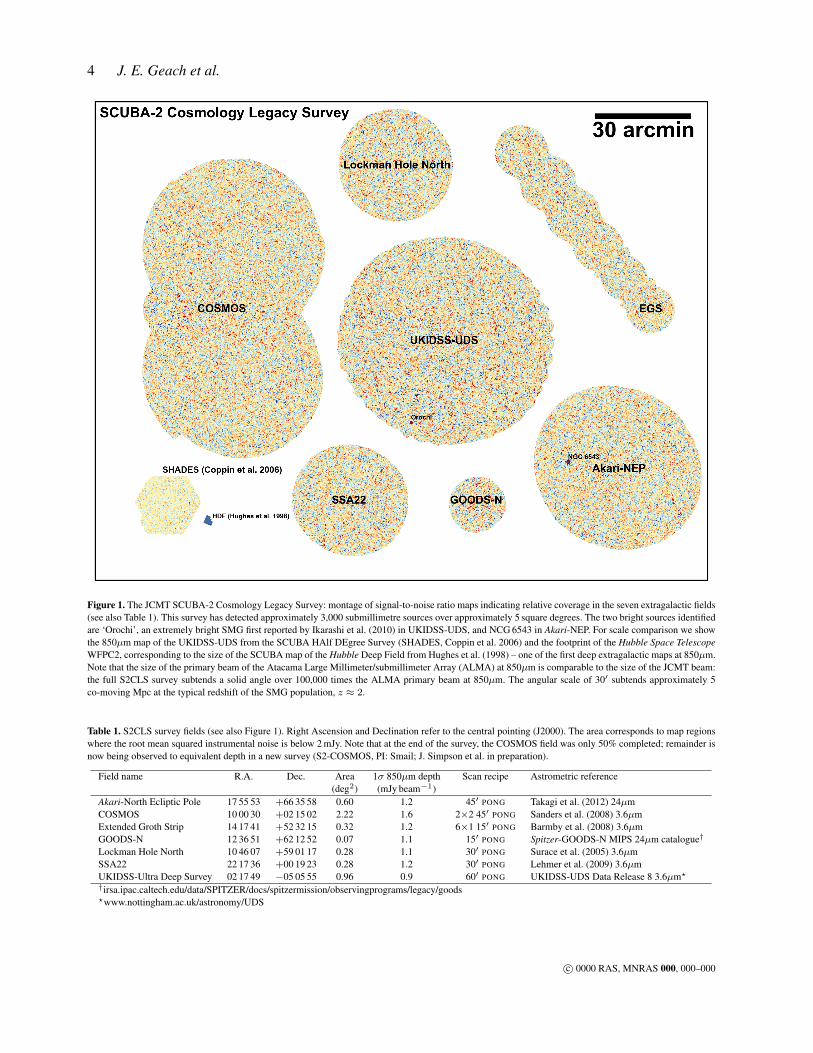
Figure 1. The JCMT SCUBA-2 Cosmology Legacy Survey: montage of signal-to-noise ratio maps indicating relative coverage in the seven extragalactic fields(see also Table 1). This survey has detected approximately 3,000 submillimetre sources over approximately 5 square degrees. The two bright sources identifiedare ‘Orochi’, an extremely bright SMG first reported by Ikarashi et al. (2010) in UKIDSS-UDS, and NCG 6543 in Akari-NEP. For scale comparison we showthe 850µm map of the UKIDSS-UDS from the SCUBA HAlf DEgree Survey (SHADES, Coppin et al. 2006) and the footprint of the Hubble Space TelescopeWFPC2, corresponding to the size of the SCUBA map of the Hubble Deep Field from Hughes et al. (1998) – one of the first deep extragalactic maps at 850µm.Note that the size of the primary beam of the Atacama Large Millimeter/submillimeter Array (ALMA) at 850µm is comparable to the size of the JCMT beam:the full S2CLS survey subtends a solid angle over 100,000 times the ALMA primary beam at 850µm. The angular scale of 30′ subtends approximately 5co-moving Mpc at the typical redshift of the SMG population, z ≈ 2.

Table 1. S2CLS survey fields (see also Figure 1). Right Ascension and Declination refer to the central pointing (J2000). The area corresponds to map regionswhere the root mean squared instrumental noise is below 2 mJy. Note that at the end of the survey, the COSMOS field was only 50% completed; remainder isnow being observed to equivalent depth in a new survey (S2-COSMOS, PI: Smail; J. Simpson et al. in preparation).

Field name R.A. Dec. Area 1σ 850µm depth Scan recipe Astrometric reference(deg2) (mJy beam−1)

Akari-North Ecliptic Pole 17 55 53 +66 35 58 0.60 1.2 45′ PONG Takagi et al. (2012) 24µmCOSMOS 10 00 30 +02 15 02 2.22 1.6 2×2 45′ PONG Sanders et al. (2008) 3.6µmExtended Groth Strip 14 17 41 +52 32 15 0.32 1.2 6×1 15′ PONG Barmby et al. (2008) 3.6µmGOODS-N 12 36 51 +62 12 52 0.07 1.1 15′ PONG Spitzer-GOODS-N MIPS 24µm catalogue†

Lockman Hole North 10 46 07 +59 01 17 0.28 1.1 30′ PONG Surace et al. (2005) 3.6µmSSA22 22 17 36 +00 19 23 0.28 1.2 30′ PONG Lehmer et al. (2009) 3.6µmUKIDSS-Ultra Deep Survey 02 17 49 −05 05 55 0.96 0.9 60′ PONG UKIDSS-UDS Data Release 8 3.6µm?†irsa.ipac.caltech.edu/data/SPITZER/docs/spitzermission/observingprograms/legacy/goods?www.nottingham.ac.uk/astronomy/UDS

c© 0000 RAS, MNRAS 000, 000–000


Nu

mb

er

of

ob

se

rva

tio

ns

05

01

00

15

0

Dec 11 Jun 12 Dec 12 Jun 13 Dec 13 Jun 14 Dec 14

Figure 2. Time distribution of 850µm observations. In total CLS con-ducted 2041 wide-field observations on 320 nights from November 2011to Febuary 2015. The increase in frequency of observations towards theend of the survey reflects the effect of ‘extended observing’ into the post-sunrise morning hours when the opacity and conditions were still suitablefor observations. Note that one observation is equivalent to 30-40 minutesof integration time.

iterative process that aims to fit the data with a model compris-ing a common-mode fluctuating atmospheric signal, positive astro-nomical signal and instrumental and fine-scale atmospheric noise.The common mode modelling is performed independently for eachSCUBA-2 sub-array, deriving a template for the average signal seenby all the bolometers. The common mode is then removed, andan extinction correction is applied (Dempsey et al. 2013). Next,a filtering step is performed in the Fourier domain, which rejectspower at frequencies corresponding to angular scales θ > 150′′

and θ < 4′′. The next step is to estimate the astrononomical signal.This is done by gridding the time-streams onto the celestial projec-tion; since each pixel will be sampled many times by independentbolometers (slewing over the sky in the PONG scanning pattern),then the positive signal in a given pixel can be taken to be an ac-curate estimate of the astronomical signal (assuming the previoussteps have eliminated all other sources of emission or spikes, etc.).This model of the astronomical signal is then projected back to atime-stream and subtracted from the data. Finally, a noise model isestimated for each bolometer by measuring the residual, which isthen used to weight the data during the mapping process in addi-tional steps. The iterative process above runs until convergence ismet. In this case, we execute a maximum of 20 iterations, or termi-nate the process when the map tolerance ∆χ2 reaches 0.05.

S2CLS obtained many individual scans of each field. TheDIMM allows for all the scans to be simultaneously reduced in themanner described above. However, we adopt an approach wherethe DIMM is only given individual observations, producing a set ofmaps for each target field which can then be co-added into a fi-nal stack. For this we use the PICARD recipe mosaic jcmt imageswhich uses the WCSMOSAIC task within the STARLINK KAPPA

package, weighting each input image by the inverse variance perpixel. With a set of individual observations for each field we canalso construct maps of sub-sets of the data and produce jackknifemaps where a random 50% of the images are inverted, thus remov-ing astronomical signal in the final stack, and generating source-free noise realisations of each field (Figure 4); useful for certainstatistical tests.

The last processing step is to apply a matched filter tothe maps, convolving with the instrumental PSF to optimizethe detection of point sources. We use the PICARD recipescuba2 matched filter which first smooths the map (and the PSF)

2h16m17m18m19m20m

Right Ascension (J2000)

30'

15'

-5°00'

-4°45'

Dec

linat

ion

(J20

00)

15 arcmin

Figure 3. An example of the sensitivity coverage in a single S2CLS field.This map shows the instrumental noise map of the UKIDSS-UDS (a sin-gle PONG), scaled between σinstr = 0.8–1.2 mJy. Contours are at steps of0.05 mJy starting at 0.8 mJy. This demonstrates the uniform nature of thePONG map over the majority of the mapping region, radially rising beyondthe nominal extent of the area scanned to uniform depth (effectively over-scan regions receiving shorter integration time).

with a 30′′ Gaussian kernel, then subtracts this from both toremove any large scale structure not eliminated in the filteringsteps that occurred during the DIMM reduction. The map is thenconvolved with the smoothed beam. A flux conversion factor of591 Jy beam−1 pW−1 is applied to give the maps units of flux den-sity. This canonical calibration is the average value derived fromobservations of hundreds of standard submillimetre calibrators ob-served during the S2CLS campaign (Dempsey et al. 2013). Thefiltering steps employed in the data reduction, including the match-filtering step, introduce a slight (10%) loss of response to pointsources. We have measured this loss by injecting a model source ofknown (bright) flux density into the data and recovering its flux af-ter filtering; we correct for this in the flux calibration. The absoluteflux calibration is expected to be accurate to within 15%.

2.3 Astrometric refinement and registration

The JCMT pointing is regularly checked against standard calibra-tors during observations, with typical pointing drift corrections typ-ically of order 1–2′′; similar to the pixel scale at which the mapsare gridded. To improve the astrometric refinement of the finalco-added maps we adopt a maximal signal-to-noise stacking tech-nique: for each field we use a mid-infrared selected catalogue andstack the submillimetre maps at the positions of reference sourcesto measure a high-significance statistical detection. We repeat theprocess many times, updating the world coordinate system refer-ence pixel coordinates at each step with small ∆α and ∆δ incre-ments. The goal is to find the (∆α, ∆δ) that maximise the signal-to-noise of the stack in the central pixel. We iterate over several lev-els of refinement until no further change in (∆α, ∆δ) is required.The average changes to the astrometric solution are of order 1–2′′,comparable to the pixel scale and similar to the source positional

c© 0000 RAS, MNRAS 000, 000–000


−5 0 5 10 15

01

23

45

Sν (mJy beam−1

)

log(N

pix)

Figure 4. Distribution of pixel values in the UKIDSS-UDS flux densitymap, showing the characteristic tail representing astronomical emission.The shaded region shows the equivalent distribution in a jackknife map,constructed by inverting a random half of the data before co-addition. Thedashed line is simply a normal distribution with zero mean and scale set tothe standard deviation of pixel values in the jackknife map, illustrating thatthe noise in the map is approximately Gaussian.

uncertainty (see §2.5.2). Table 1 lists the reference catalogues usedfor each field.

2.4 Statistics

2.4.1 Area coverage

The PONG scanning strategy results in maps that are uniformlydeep over the nominal scanning area, however the usable area ineach map is larger than this because of overscan, with radially in-creasing noise due to the lower effective exposure time in theseregions. Although shallower than the map centres, these annularregions around the perimeters of the fields, are deep enough to de-tect sources. Figure 5 shows the cumulative area of the survey as afunction of (instrumental) noise. The total survey area is approxi-mately 5 square degrees, with >90% of the survey area reaching asensitivity of under 2 mJy beam−1.

2.4.2 Modelling the PSF

The matched-filtering step described in §2.2 modifies the shape ofthe instrumental PSF, effectively slightly broadening it and increas-ing the depth of bowling. We derive an empirical PSF by stacking322 >5σ significance point sources in the UKIDSS-UDS map andfit an analytic surface function to the average profile. The profile isshown in Figure 6 in comparison to the instrumental PSF, and hasa FWHM of 14.8′′. Two-dimensional fitting of the stack reveals thatthe beam profile P (θ) is circular to within 1% and can be fit withthe superposition of two Gaussian functions:

P (θ) = A exp

(θ2

2σ2

)− 0.98A exp

(θ2

2.04σ2

)(1)

1.0 1.5 2.0 2.5 3.0

01

23

45

6

SHADES

Coppin et al. (2006)

LESS

Weiss et al. (2009)

σrms (mJy beam−1

)

Ω(σ

<σ

rms)

(degre

e2)

Figure 5. Cumulative area of the SCUBA-2 Cosmology Legacy Survey asa function of sensitivity, compared to the largest previous 850µm surveysSHADES (Coppin et al. 2006) and (at 870µm) LESS (Weiss et al. 2009).The majority of S2CLS reaches a sensitivity of below 2 mJy beam−1, adramatic step forward compared to previous surveys in the same waveband.

with A = 41.4 and σ = 9.6′′.

2.4.3 The confusion limit

The confusion limit (Scheuer 1957) σc is the flux level at whichthe pixel-to-pixel variance σ2 no longer reduces with exposuretime due to crowding of the beam by faint sources. The total vari-ance is a combination of the instrumental noise σi (in units ofmJy beam−1√s) and the confusion noise (in units of mJy beam−1):

σ2 = σ2i t−1 + σ2

c . (2)

We can evaulate the confusion limit by measuring σ2 directly fromthe pixel data in a progression of maps as we sequentially co-addnew scans. Figure 7 shows how the variance evolves as a functionof inverse pixel integration time for the central 15′ of the UKIDSS-UDS, which reaches an instrumental noise of 0.8 mJy beam−1. Thebest fit σc is 0.8 mJy beam−1; this confusion noise should be addedin quadrature to instrumental and deboosting (§2.5.1) uncertaintieswhen considering the flux density of sources.

2.5 Source extraction

The matched-filtering step optimises the maps for the detection ofpoint sources – i.e. emission features identical to the PSF. To extractand catalogue sources we employ a simple top-down peak-findingalgorithm: starting from the most significant peak in the signal-to-noise ratio map, the peak flux, noise and position of a source iscatalogued before the source is removed from the flux (and signal-to-noise) map by subtracting a scaled version of the model PSF.The highest peak in the source-subtracted map is then cataloguedand subtracted and so-on until a floor threshold significance isreached, below which ‘detections’ are no longer trusted. Note that

c© 0000 RAS, MNRAS 000, 000–000


−40 −30 −20 −10 0 10 20 30 40

−0

.20

.00.2

0.4

0.6

0.8

1.0

θ (arcseconds)

Flu

x (

no

rm)

Figure 6. Model of the SCUBA-2 PSF. The dashed line shows the instru-mental PSF (Dempsey et al. 2013), and the points show the shape of theaverage point source in the UKIDSS-UDS field, derived by stacking allsources detected at 5σ significance or greater. The maps are match-filtered,which includes a smoothing step that slightly broadens the instrumental PSFand deepens ‘ringing’. The empirical PSF is well modelled with the super-position of two Gaussians (§2.3.2), is circular, and has a FWHM of 14.8′′.

this procedure can potentially deblend sources with markedly dif-ferent fluxes. The floor detection limit is set to 3σ which allows usto explore the properties of the lowest-significance detections, not-ing that further cutting can be performed directly on the catalogue.In the following we assume a cut of 3.5σ as the formal detectionlimit of S2CLS, where we estimate that the false detection rate isapproximately 20% (see §2.5.3).

2.5.1 Completeness and flux boosting

To evaluate source detection completeness we insert fake sourcesmatching a realistic number count distribution into the jackknifenoise maps of each field and then try to recover them using thesource detection algorithm described above. We adopt the differ-ential number counts fit of Casey et al. (2013) as a fiducial model,which has the Schechter form:

dN

dS=

(N0

S0

)(S

S0

)−γexp

(− S

S0

)(3)

with N0 = 3300 deg−2, S0 = 3.7 mJy and γ = 1.4. We in-sert sources down to a flux density limit of 1 mJy and each sourceis placed at a random position into each map (we do not encodeany clustering of the injected sources). An injected source is re-covered if a point source is found above the detection thresholdwithin 1.5×FWHM of the input position. This is a somewhat ar-bitrary, but generous, threshold, and if there are multiple injectedsources within this radius, then we take the closest match. Thisprocedure is repeated 5,000 times for each map, generating a setof mock catalogues containing millions of sources with a realisticflux distribution, allowing us to assess the completeness and fluxboosting statistics.

The ratio of recovered sources to total number of input sources

01

23

0 1 2 3

t−1

(10−3

seconds−1

)

σ2 (

mJy b

eam

−1)2

Observed noise

Pure instrumental noise

Figure 7. Measurement of the 850µm confusion limit for SCUBA-2: weprogressively co-add single exposures of the UKIDSS-UDS field, mea-suring the pixel-to-pixel root mean square value in the uniform central15′ of the beam-convolved flux map, whilst also tracking the fall off inthe pure instrumental noise estimate. At infinite exposure the instrumentalnoise is projected to reach zero, whereas the non-zero intercept of the ob-served flux r.m.s. is the confusion limit (Equation 2). We measure this to beσc ≈ 0.8 mJy beam−1 averaged over the field. Note that the exposure timeis the average per 2′′ pixel.

Table 2. 50% and 80% completeness limits for the S2CLS fields, quotedat the median map depth (Table 1). We also present the number of sourcesbrighter than the 50% and 80% limits in each field (N50,80). Note that theseflux densities refer to the deboosted – i.e. intrinsic – flux densities. At the 5σlevel observed flux densities are typically overestimated by 20% (§2.5.1).

Field 50% 80% N50 N80

(mJy) (mJy)Akari-NEP 4.1 5.2 132 59UKIDSS-UDS 3.0 3.8 543 302COSMOS 4.9 6.2 302 181Lockman Hole North 3.6 4.6 96 49GOODS-N 3.9 4.7 32 21Extended Groth Strip 3.9 5.0 99 51SSA22 3.9 4.9 78 38

is evaluated in bins of input flux density and local (instrumental)noise. When applying completeness corrections we use the binnedvalues as a look-up table, using two dimensional spline interpola-tion to estimate the completeness rate for a given source. Figure 8compares the average completeness of each field (i.e. at the averagedepth of each map) as a function of intrinsic flux density. Table 2lists the average 50% and 80% completeness limits for each fieldand the number of sources above each limit.

We can simultaneously evaluate flux boosting as a functionof local noise and observed flux density simply by comparing therecovered flux to the input flux density of each source. Flux boost-ing is the overestimation of source flux when measurements aremade in the presence of noise and is related to both Eddington and

c© 0000 RAS, MNRAS 000, 000–000


0 1 2 3 4 5 6 7 8 9 10

0.0

0.2

0.4

0.6

0.8

1.0

Co

mp

lete

ne

ss

S850 (mJy)

UDSAkari−NEPEGSGOODS−NLockman Hole NorthCOSMOSSSA22

Figure 8. Completeness of the different S2CLS fields, derived from therecovery rate of fake sources injected into jackknife maps as a function ofinput flux, where a successful recovery at a detection significance of 3.5σ.Note that the completeness falls to zero at 1 mJy as this corresponds tothe limit of the injected source model; in practice it is possible that sub-mJy sources could be boosted above the detection limit. The 50% and 80%limits of each field are listed in Table 2.

Malmquist bias. Due to the statistical nature of boosting, a sourcewith some observed flux density Sobs is actually drawn from a dis-tribution of true flux density, p(Strue). Our recovery procedure al-lows us to estimate p(Strue), since we can simply measure the his-togram of the injected flux density of sources in bins of (Sobs, σ).This method can be compared to the traditional Bayesian techniqueto estimate boosting (e.g. Jauncey et al. 1968; Coppin et al. 2005),such that the posterior probability distribution for an observed fluxdensity can be expressed:

p(Strue|Sobs, σ) =p(Strue)p(Sobs, σ|Strue)

p(Sobs, σ). (4)

The likelihood of the data is given by assuming a Gaussian pho-tometric error on the observed flux density, and the prior is sim-ply the same assumed number counts model used in the simula-tions described above. Figure 9 compares the empirically-estimatedp(Strue) and the posterior probability distribution for Strue fromEquation (4). The empirical distributions are truncated at 1 mJybecause this is the faint limit of the injected source distribution;clearly we can not track individual sources fainter than this. Anidentical counts model is used as a prior in the Bayesian approach,but note that the posterior flux density distribution does extend be-low 1 mJy; this is because it is effectively the product of a Gaus-sian (the observed flux density and instrumental uncertainty) andthe histogram of pixel values in a map of sources drawn from themodel number counts, convolved with the beam. The two meth-ods return similar results, although the empirical method systemat-ically predicts a slightly smaller boosting factor B = Sobs/Strue

than the Bayesian approach, with the two methods converging asSobs increases. Note that neither method assumes any clustering ofsources, which could well be important (Hodge et al. 2013; Simp-son et al. 2015).

There are two important differences in the deboosting methodsthat may explain this: (i) the Bayesian approach does not considernoise (aside from the confusion noise arising from convolving thefake map with the beam), and, related, (ii) the posterior flux distri-bution derived in Equation 4 is not necessarily measured ‘at peak’,i.e. does not consider that the recovered position of a source canshift due to the presence of noise; in the empirical method, we ac-count for such shifts. This relates to the ‘bias-to-peak’ discussedby Austermann et al. (2010). We adopt the ‘empirical’ approach inthis work to deboost observed fluxes: we draw samples from thedistribution of Strue for a given (Sobs, σ) and calculate the meanand variance of these true fluxes, with the latter providing the un-certainty on the deboosted flux density (provided in the source cat-alogue). We summarise the empirically derived completeness andboosting for each field, visualised in the plane of flux density andlocal instrumental noise, in Figure 10. In Figure 11 we show theaverage flux boosting as a function of signal-to-noise ratio in eachfield, indicating that at fixed detection significance, the level of fluxboosting is consistent across the survey, with observed flux densi-ties approximately 20% higher on average than the intrinsic fluxdensity at the 5σ level. The average boosting is well described by apower law:

B = 1 + 0.2

(SNR

5

)−2.3

(5)

2.5.2 Positional uncertainty

The simulations described above allow us to investigate the scatterin the difference between input position and recovered position.Like the completeness and boosting, we evaluate the average δθbetween input and recovered position in bins of input flux densityand local instrumental noise. Following Condon et al. (2007) andIvison et al. (2007), for a given (Gaussian-like) beam, the positionalaccuracy is expected to scale with signal-to-noise. Figure 12 showsthe mean difference between input and recovered source positionas a function of signal-to-noise ratio for each field. We find thatthe positional uncertainty of S2CLS sources is well described bya simple power law, reminiscent of Equation B22 of Ivison et al.(2007):

δθ = 1.2′′ ×(

SNR

5

)−1.6

(6)

2.5.3 False detection rate

To measure the false detection rate we compare the number of ‘de-tections’ in the jackknife maps to those in the real maps as a func-tion of signal-to-noise ratio. By construction, the jackknife mapscontain no astronomical signal and have Gaussian noise properties(Figure 4); therefore any detections are due to statistical fluctua-tions expected from Gaussian noise at the >3.5σ level. Figure 13shows the false detection rate as a function signal-to-noise ratio; Atour 3.5σ limit the false detection (or contamination) rate is 20%,falling to 6% at 4σ and falls below 1% for a >5σ cut. The falsedetection rate follows

log10(F) = 2.67− 0.97× SNR. (7)

Equation 7 implies that caution should be taken when consideringindividual sources in the S2CLS catalogue at detection significanceof less than 5σ; follow-up confirmation and/or robust counterpartidentification will be important for assessing the reality of sources

c© 0000 RAS, MNRAS 000, 000–000


3.5 mJy 4.0 mJy 4.5 mJy 5.0 mJy 5.5 mJy 6.0 mJy

6.5 mJy

Sν (mJy beam−1

)0

Sν (mJy beam−1

)5

Sν (mJy beam−1

)10

Sν (mJy beam−1

)15

Sν (mJy beam−1

)Sν (mJy beam−1

)

0.0

0

P(S

ν)

0.2

5

P(S

ν)

0.5

0

P(S

ν)

P(S

ν)

7.0 mJy 7.5 mJy 8.0 mJy 8.5 mJy 9.0 mJy

Figure 9. Comparison of deboosted flux density distributions for a Bayesian and empirical ‘recovery’ method (§2.5.1), using the UKIDSS-UDS field as anexample. Both deboosting methods involve considering a model source distribution (down to a flux density of 1 mJy in this case). Each panel shows an observedflux probability distribution, assuming Gaussian uncertainties, for increasing observed flux. The solid and hatched distributions show the predicted intrinsicflux distribution for the Bayesian and direct methods respectively. In general the average boosting measured by the two methods agree well, converging asobserved flux density increases, however the ‘direct’ method systematically predicts less boosting compared to the Bayesian approach; we discuss this in themain text.

detected close to the survey limit, and this work has already begun(e.g. Chen et al. 2016).

3 NUMBER COUNTS OF THE 850µM POPULATION

In Table 4 we present a sample of the S2CLS catalogue. Thefull catalogue contains 2,851 sources at a detection significance of>3.5σ. The catalogue contains observed and deboosted flux densi-ties, instrumental and deboosted flux density uncertainties, and in-dividual completeness and false detection rates. The full catalogueand maps (match-filtered and non-match-filtered) are available atthe DOI: http://dx.doi.org/10.5281/zenodo.57792

The surface density of sources per observed flux density in-terval dN/dS – of a cosmological population is a simple measureof source abundance and a powerful tool for model comparisons.To measure the counts, for each catalogued source we first deboostthe observed flux density using the empirical approach describedin §2.5.1, and then apply the corresponding completeness correc-tion for the deboosted (i.e. ‘true’) flux density. When deboosting,we consider the full intrinsic flux distribution as estimated by oursimulation, accounting for the fact that a range of intrinsic flux den-sities can map onto an observed flux density. Therefore, we evaluatedN/dS 1000 times; in each calculation every source is deboostedby randomly sampling the intrinsic flux distribution and complete-ness correcting each deboosted source accordingly. We take themean of these 1000 realisations as the final number counts, withthe standard deviation of dN/dS in each bin as an additional uncer-tainty (to the Poisson error). We make a correction for each sourcebased on the probability it is a false positive, using the empiricaldetermination described in §2.5.3.

While the various corrections are intended to recover the ‘true’underlying source distribution, it is important to confirm if any sys-tematic biases remain, since the procedure for actually identifyingsources is imperfect, as is the ‘recovery’ of injected model sourcesused to estimate flux boosting and completeness. To examine thiswe inject three different source count models into a jackknife noisemap (of the UKIDSS-UDS field). One model is identical to the

Schechter form used in §2.6.1 (Equation 3); in the other two mod-els we simply adjust the faint end slope to γ = 0.4 and γ = 2.4,keeping the other parameters fixed. With knowledge of the exactmodel counts injected into the map, we can compare to the recov-ered counts before and after corrections have been applied. Figure14 shows ([dN/dS]rec− [dN/dS]true)/[dN/dS]true for the threemodels before and after corrections. In the absence of correction,flux boosting tends to result in the systematic overestimation of thenumber counts in all but the faintest flux bin, where incompletenessdominates, and the overestimation increases with increasing γ, asexpected. After the corrections have been applied, there remains aslight underestimation in the counts in the faintest bin (3–4 mJy) atthe 10% level, but in general the corrected ‘observed’ counts are inexcellent agreement with the input model. The origin for the slightdiscrepancy is not clear, but it is likely that it simply stems fromsubtle effects not modelled well by our recovery simulation, and inparticular what consititutes a ‘recovered’ source. One can observea systematic effect that the γ = 2.4 and γ = 0.4 models are over-and under-estimated (respectively) at approximately the 10% levelfor the full observed flux range, but this is not a significant sys-tematic uncertainty compared to shot noise expected from Poissonstatistics. Given that the fiducial model we use in the complete-ness simulation is based on observed 850µm number counts, andthe γ = 2.4 and γ = 0.4 models are rather extreme compared toempirical constraints, we consider this test as an adequate demon-stration that our measured number counts are robust. Nevertheless,we apply a simple correction to the observed corrected counts byfitting a spline to the residual model counts in Figure 14 and applythis as a ‘tweak’ factor to the number counts on a bin-by-bin basis.

The S2CLS differential (and cumulative) number counts arepresented in Table 4 and Figure 15. Tables of the number countsof individual fields are available in the electronic version of the pa-per. S2CLS covers a solid angle large enough to detect reasonablenumbers of the rarer, bright sources at S850 > 10 mJy, allowing usto robustly measure the bright end of the observed 850µm numbercounts. As a guide, there are about ten sources with flux densitiesgreater than 10 mJy per square degree. The 850µm source countsabove 10 mJy clearly show an upturn in source density that is due to

c© 0000 RAS, MNRAS 000, 000–000


1.5

1.5

2 2.5 3 3.5 4

4.5

5

0 5 10

1.0

1.2

Input Sν (mJy)

σ ins

t (m

Jy)

UDS

0.05

0.1

0

.2

0.3

0

.4

0.5

0

.6

0.7

0.8

0.9

0

.95

0 5 10

1.0

1.2

Input Sν (mJy)

σ ins

t (m

Jy)

1.05

1.1 1.15

1.2

1.2

1.2

5

1.2

5

1.3

1.3

1.3

5 1

.4

0 5 10

1.0

1.2

Observed Sν (mJy)

σ ins

t (m

Jy)

1 1.5 2 2.5 3 3.5

4

4.5

0 5 10

1.2

1.4

Input Sν (mJy)

σ ins

t (m

Jy)

Akari−NEP

0.0

5

0.1

0.2

0

.3

0.4 0

.5

0.6

0.7

0.8

0.9

0

.95

0 5 10

1.2

1.4

Input Sν (mJy)

σ ins

t (m

Jy)

1.05

1.1

1.1

5

1.2

1.2

5

1.3

1.3

1

.3

1.35

1.3

5

1.3

5

1.4

1.4

1.4

1.45

0 5 10

1.2

1.4

Observed Sν (mJy)

σ ins

t (m

Jy)

1.5 2 2.5 3

3.5

4

4

4.5

5

0 5 10

0.8

1.0

1.2

1.4

1.6

1.8

2.0

Input Sν (mJy)

σ ins

t (m

Jy)

COSMOS

0.0

1

0.05

0.1 0

.2

0.3

0.4

0.5

0.6

0

.7

0.8

0.9

0.9

5

0 5 10

0.8

1.0

1.2

1.4

1.6

1.8

2.0

Input Sν (mJy)

σ ins

t (m

Jy)

1.05

1.1

1.15

1.2

1.25

1.3

1.3

1.35

1.4

1.4

1.4

5

1.5

0 5 10

0.8

1.0

1.2

1.4

1.6

1.8

2.0

Observed Sν (mJy)

σ ins

t (m

Jy)

1

1.5

2 2.5 3 3.5 4

0 5 10

1.0

1.2

1.4

Input Sν (mJy)

σ ins

t (m

Jy)

Lockman Hole North

0.0

5 0

.1

0.2

0

.3

0.4

0

.5

0.6

0

.7

0.8

0

.9

0.9

5

0 5 10

1.0

1.2

1.4

Input Sν (mJy)

σ ins

t (m

Jy)

1.05

1.1 1.15

1.2 1.25

1.3

1.3

1

.35

1.35

1.35

1.4

1.4

1.4

0 5 10

1.0

1.2

1.4

Observed Sν (mJy)

σ ins

t (m

Jy)

Figure 10. Two dimensional visualisations of the results of the recovery simulation in each field. The first column shows the number of artificial sourcesinjected per bin of input flux density and local instrumental noise (labels are log10(N)). The prominent horizontal ridges clearly show the typical depth of themap. The middle column shows the completeness as a function of true flux density and local instrumental noise and the last column shows the average fluxboosting as a function of observed flux density and local instrumental noise. The dashed line shows the 3.5σ detection limit.

c© 0000 RAS, MNRAS 000, 000–000


1.5

2

2.5 3

3.5

4

4

4

0 5 10

1.0

1.2

1.4

1.6

Input Sν (mJy)

σ ins

t (m

Jy)

EGS

0.0

5

0.1

0.2

0.3

0.4

0.5

0.6

0

.7

0.8

0.9

0.9

5

0 5 10

1.0

1.2

1.4

1.6

Input Sν (mJy)

σ ins

t (m

Jy)

1.05

1.1

1.15 1.2 1.25

1.2

5

1.3

1.3

5

1.4

1.45

0 5 10

1.0

1.2

1.4

1.6

Observed Sν (mJy)

σ ins

t (m

Jy)

1

1.5 2 2.5 3 3.5

4

0 5 10

1.2

1.4

Input Sν (mJy)

σ ins

t (m

Jy)

SSA22

0.0

5

0.1

0.2

0.3

0.4

0.5

0

.6

0.7

0.8

0.9

0.9

5 0 5 10

1.2

1.4

Input Sν (mJy)

σ ins

t (m

Jy)

1.05

1.1

1.1

5 1.2

1.25

1.3

1.3

1.3

1.3

1.3

1.35

1.3

5

1.4 1.4

0 5 10

1.2

1.4

Observed Sν (mJy)

σ ins

t (m

Jy)

1

1.5 2 2.5 3 3.5

0 5 10

1.0

1.2

1.4

Input Sν (mJy)

σ ins

t (m

Jy)

GOODS−N

0.0

1 0

.05

0.1

0.2

0.3

0.4

0

.5

0.6

0.7

0.8

0.9

0

.95

0 5 10

1.0

1.2

1.4

Input Sν (mJy)

σ ins

t (m

Jy)

1.05 1.1 1.15

1.2 1.25

1.3

1.3

1.3

1.3

1.3

5

1.35

1.3

5

1.4

1.45

0 5 10

1.0

1.2

1.4

Observed Sν (mJy)

σ ins

t (m

Jy)

Figure 10. (continued)

a mixture of local emitters and gravitationally lensed sources2. Thewide area counts of Herschel demonstrated the same (predicted)phenomenon in the SPIRE bands (Negrello et al. 2010), and it hassince been demonstrated that a simple bright submillimetre flux cutis highly effective at identifying strongly lensed sources once lo-cal galaxies have been rejected. The effect has already been ob-served in the millimetre regime: Vieira et al. (2010) detect the up-turn in the 1.4 mm counts at S1.4mm > 10 mJy from SPT over a87 deg2 survey, and Scott et al. (2012) have reported tentative ev-idence of an upturn in the counts at 1.1 mm at S1.1mm > 13 mJywith AzTEC over 1.6 deg2. Much larger 850µm surveys (exceeding10 deg2) could utlize a similar selection to cleanly identify lensed850µm-selected high-redshift galaxies.

2 Note that the Akari-NEP field contains the galactic object NGC 6543 (theCat’s Eye Nebula) - which is a ∼200 mJy 850µm source

The S2CLS number counts are in reasonable agreement withprevious surveys for the flux range probed (for clarity, a non-exhaustive list of previous surveys, including recent SCUBA-2 re-sults, are shown in Figure 15: Coppin et al 2006; Weiss et al. 2009;Casey et al. 2013; Chen et al. 2013), but with the large numberof sources in S2CLS we can dramatically reduce the Poisson er-rors: in the faintest bin the Poisson uncertainty on the differen-tial counts over the whole survey is just ∼4%. We fit the com-bined differential counts (up to 20 mJy after which the local/lensingupturn starts to contribute significantly) with the Schechter func-tional form given in Equation 3. We find the best fit parametersN0 = 7180 ± 1220 deg−2, S0 = 2.5 ± 0.4 mJy beam−1 andγ = 1.5± 0.4.

c© 0000 RAS, MNRAS 000, 000–000


Table 3. Sample of the full S2CLS catalogue, listing the highest and lowest significance detections in each field. Coordinates are J2000, with the individualmap astrometric solutions tied to the reference catalogue listed in Table 1. The Sobs

850 ± σinst column gives the observed flux density and instrumental noise,S/N gives the detection signal-to-noise ratio, and S850 ± σtot gives the estimated true flux density and combined total (instrumental, deboosting, confusion)uncertainty. The final column log10(F) is the logarithm of the false detection rate for the detection signal-to-noise ratio (Equation 7), negligible for brightsources, but important to consider for sources at the detection limit.

S2CLS ID Short name R.A. Dec. Sobs850 ± σinst S/N S850 ± σtot 〈C〉 log10(F)

S2CLSJ175833+663757 NEP.0001 17 58 33.60 +66 37 57.7 195.4± 1.2 158.4 195.4± 1.5 1.00 −147.78S2CLSJ175416+665117 NEP.0329 17 54 16.57 +66 51 17.0 4.3± 1.2 3.5 2.9± 1.9 0.25 −0.66S2CLSJ100015+021548 COS.0001 10 00 15.72 +02 15 48.6 12.9± 0.8 15.2 12.9± 1.2 1.00 −11.78

S2CLSJ095936+022506 COS.0733 09 59 36.09 +02 25 06.5 5.4± 1.5 3.5 3.6± 2.4 0.25 −0.65S2CLSJ141951+530044 EGS.0001 14 19 51.56 +53 00 44.8 16.3± 1.2 14.1 16.3± 1.4 1.00 −10.69S2CLSJ141612+521316 EGS.0227 14 16 12.05 +52 13 16.8 3.7± 1.0 3.5 2.6± 1.7 0.28 −0.66S2CLSJ123730+621258 GDN.0001 12 37 30.73 +62 12 58.5 12.8± 1.0 13.2 11.9± 1.6 1.00 −9.82S2CLSJ123734+620736 GDN.0068 12 37 34.33 +62 07 36.5 5.0± 1.4 3.5 3.3± 2.2 0.23 −0.65S2CLSJ104635+590748 LHO.0001 10 46 35.78 +59 07 48.0 12.0± 1.0 11.6 11.5± 1.8 0.99 −8.31S2CLSJ104541+584640 LHO.0219 10 45 41.47 +58 46 40.0 4.1± 1.2 3.5 3.0± 1.8 0.29 −0.67S2CLSJ221732+001740 SSA.0001 22 17 32.50 +00 17 40.4 14.5± 1.1 13.0 14.5± 1.4 0.96 −9.72S2CLSJ221720+002024 SSA.0198 22 17 20.23 +00 20 24.4 3.9± 1.1 3.5 2.8± 1.8 0.28 −0.65S2CLSJ021830-053130 UDS.0001 02 18 30.77 −05 31 30.8 52.7± 0.9 56.7 52.7± 1.2 1.00 −51.18S2CLSJ021823-051508 UDS.1080 02 18 23.12 −05 15 08.9 3.1± 0.9 3.5 2.4± 1.5 0.30 −0.65

Bo

ost

= R

ecove

red

/ I

np

ut

flu

x d

en

sity

Signal−to−noise S850 σinst

3 4 5 6 7 8 9 10

1.0

01

.20

1.4

01

.60


Figure 11. Average flux boosting as a function of signal-to-noise ratio,showing consistency at a fixed signal-to-noise level across different fields.The boosting can be described by a power law, however in practice we de-boost sources individually based on their observed flux density and localinstrumental noise, and drawing on the full probability distribution of trueflux densities derived from our recovery simulation.

3.1 Field-to-field variance

Taking the full survey counts as an average measure of the abun-dance of submillimetre sources, with S2CLS we can now inves-tigate field-to-field variance in the number counts in a consistentmanner; this is important given that SMGs are thought to be ahighly biased tracer of the matter field (Hickox et al. 2012; Chen etal. 2016). Letting ρ(S) = N(> S), for each field we can con-sider the deviation of the counts compared to the mean densityper flux bin: δ(S) = (ρ(S) − 〈ρ(S)〉)/〈ρ(S)〉. In Figure 16 weshow the δ(S) measured for each field as a function of flux den-sity, where uncertainties are the combined Poisson errors (obvi-

Po

sitio

na

l e

rro

r (a

rcse

co

nd

s)



3 4 5 6 7 8 9 10

0.0

0.5

1.0

1.5

2.0

2.5

3.0

Figure 12. Average positional error based on the difference between inputand recovered (peak) position from our recovery simulation. All fields fol-low a similar trend, with the positional uncertainty decreasing with increas-ing source significance. We fit the uncertainties with a simple power law toestimate the 1σ positional uncertainty as a function of observed signal-to-noise ratio (§2.5.2).

ously dominated by the single field counts). The field-to-field scat-ter on ∼0.5–1 degree scales is generally within 50% of the survey-averaged density and reasonably consistent with the Poisson errors.There are some hints that the GOODS-N field has a slightly ele-vated density compared to the mean (hints that were already appar-ent in the original SCUBA maps of this field, see Borys et al. 2002;Pope et al. 2005; Coppin et al. 2006), but this is marginal given thePoisson errors. However, to explore this further, and to quantify thesignificance of any overdensity, we can evaluate the field-to-fieldfluctuations on scales equivalent to the GOODS-N field taking intoaccount cosmic variance.

Field-to-field variance in the observed number counts is

c© 0000 RAS, MNRAS 000, 000–000


11

01

00

3.0 3.5 4.0 4.5 5.0

Fa

lse

de

tectio

ns (

%)


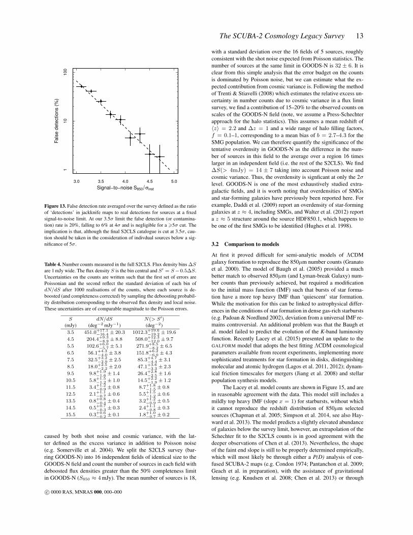
Figure 13. False detection rate averaged over the survey defined as the ratioof ‘detections’ in jackknife maps to real detections for sources at a fixedsignal-to-noise limit. At our 3.5σ limit the false detection (or contamina-tion) rate is 20%, falling to 6% at 4σ and is negligible for a >5σ cut. Theimplication is that, although the final S2CLS catalogue is cut at 3.5σ, cau-tion should be taken in the consideration of indivdual sources below a sig-nificance of 5σ.

Table 4. Number counts measured in the full S2CLS. Flux density bins ∆Sare 1 mJy wide. The flux density S is the bin central and S′ = S−0.5∆S.Uncertainties on the counts are written such that the first set of errors arePoissonian and the second reflect the standard deviation of each bin ofdN/dS after 1000 realisations of the counts, where each source is de-boosted (and completeness corrected) by sampling the deboosting probabil-ity distribution corresponding to the observed flux density and local noise.These uncertainties are of comparable magnitude to the Poisson errors.

S dN/dS N(> S′)(mJy) (deg−2 mJy−1) (deg−2)3.5 451.0+17.1

−16.4 ± 20.3 1012.3+19.6−19.2 ± 19.6

4.5 204.4+9.3−8.9 ± 8.8 508.0+12.3

−12.0 ± 9.7

5.5 102.6+6.0−5.7 ± 5.1 271.9+8.5

−8.2 ± 6.5

6.5 56.1+4.3−4.0 ± 3.8 151.8+6.2

−6.0 ± 4.3

7.5 32.5+3.2−2.9 ± 2.5 85.3+4.7

−4.4 ± 3.1

8.5 18.0+2.5−2.2 ± 2.0 47.1+3.6

−3.3 ± 2.3

9.5 9.8+1.9−1.6 ± 1.4 26.4+2.8

−2.5 ± 1.6

10.5 5.8+1.5−1.2 ± 1.0 14.5+2.2

−1.9 ± 1.2

11.5 3.4+1.2−0.9 ± 0.8 8.7+1.8

−1.5 ± 0.8

12.5 2.1+1.1−0.7 ± 0.6 5.5+1.5

−1.2 ± 0.6

13.5 0.8+0.8−0.4 ± 0.4 3.2+1.2

−0.9 ± 0.5

14.5 0.5+0.7−0.3 ± 0.3 2.4+1.1

−0.8 ± 0.3

15.5 0.3+0.6−0.2 ± 0.1 1.8+1.0

−0.7 ± 0.2

caused by both shot noise and cosmic variance, with the lat-ter defined as the excess variance in addition to Poisson noise(e.g. Somerville et al. 2004). We split the S2CLS survey (bar-ring GOODS-N) into 16 independent fields of identical size to theGOODS-N field and count the number of sources in each field withdeboosted flux densities greater than the 50% completeness limitin GOODS-N (S850 ≈ 4 mJy). The mean number of sources is 18,

with a standard deviation over the 16 fields of 5 sources, roughlyconsistent with the shot noise expected from Poisson statistics. Thenumber of sources at the same limit in GOODS-N is 32 ± 6. It isclear from this simple analysis that the error budget on the countsis dominated by Poisson noise, but we can estimate what the ex-pected contribution from cosmic variance is. Following the methodof Trenti & Stiavelli (2008) which estimates the relative excess un-certainty in number counts due to cosmic variance in a flux limitsurvey, we find a contribution of 15–20% to the observed counts onscales of the GOODS-N field (note, we assume a Press-Schechterapproach for the halo statistics). This assumes a mean redshift of〈z〉 = 2.2 and ∆z = 1 and a wide range of halo filling factors,f = 0.1–1, corresponding to a mean bias of b = 2.7–4.3 for theSMG population. We can therefore quantify the significance of thetentative overdensity in GOODS-N as the difference in the num-ber of sources in this field to the average over a region 16 timeslarger in an independent field (i.e. the rest of the S2CLS). We find∆S(> 4mJy) = 14 ± 7 taking into account Poisson noise andcosmic variance. Thus, the overdensity is signficant at only the 2σlevel. GOODS-N is one of the most exhaustively studied extra-galactic fields, and it is worth noting that overdensities of SMGsand star-forming galaxies have previously been reported here. Forexample, Daddi et al. (2009) report an overdensity of star-forminggalaxies at z ≈ 4, including SMGs, and Walter et al. (2012) reporta z ≈ 5 structure around the source HDF850.1, which happens tobe one of the first SMGs to be identified (Hughes et al. 1998).

3.2 Comparison to models

At first it proved difficult for semi-analytic models of ΛCDMgalaxy formation to reproduce the 850µm number counts (Granatoet al. 2000). The model of Baugh et al. (2005) provided a muchbetter match to observed 850µm (and Lyman-break Galaxy) num-ber counts than previously achieved, but required a modificationto the initial mass function (IMF) such that bursts of star forma-tion have a more top heavy IMF than ‘quiescent’ star formation.While the motivation for this can be linked to astrophysical differ-ences in the conditions of star formation in dense gas-rich starbursts(e.g. Padoan & Nordlund 2002), deviation from a universal IMF re-mains controversial. An additional problem was that the Baugh etal. model failed to predict the evolution of the K-band luminosityfunction. Recently Lacey et al. (2015) presented an update to theGALFORM model that adopts the best fitting ΛCDM cosmologicalparameters available from recent experiments, implementing moresophisticated treatments for star formation in disks, distinguishingmolecular and atomic hydrogen (Lagos et al. 2011, 2012); dynam-ical friction timescales for mergers (Jiang et al. 2008) and stellarpopulation synthesis models.

The Lacey et al. model counts are shown in Figure 15, and arein reasonable agreement with the data. This model still includes amildly top heavy IMF (slope x = 1) for starbursts, without whichit cannot reproduce the redshift distribution of 850µm selectedsources (Chapman et al. 2005; Simpson et al. 2014, see also Hay-ward et al. 2013). The model predicts a slightly elevated abundanceof galaxies below the survey limit, however, an extrapolation of theSchechter fit to the S2CLS counts is in good agreement with thedeeper observations of Chen et al. (2013). Nevertheless, the shapeof the faint end slope is still to be properly determined empirically,which will most likely be through either a P(D) analysis of con-fused SCUBA-2 maps (e.g. Condon 1974; Pantanchon et al. 2009;Geach et al. in preparation), with the assistance of gravitationallensing (e.g. Knudsen et al. 2008; Chen et al. 2013) or through

c© 0000 RAS, MNRAS 000, 000–000


3 4 5 6 7 8 9 10

−0

.75

−0

.25

0.2

50

.75

Sν (mJy)

((dN

dS

) ou

t−

(dN

dS

) tru

e)

(dN

dS

) tru

e

γ = 0.4

γ = 1.4

γ = 2.4

3 4 5 6 7 8 9 10

−0

.75

−0

.25

0.2

50

.75

Sν (mJy)

((dN

dS

) ou

t−

(dN

dS

) tru

e)

(dN

dS

) tru

e

γ = 0.4

γ = 1.4

γ = 2.4

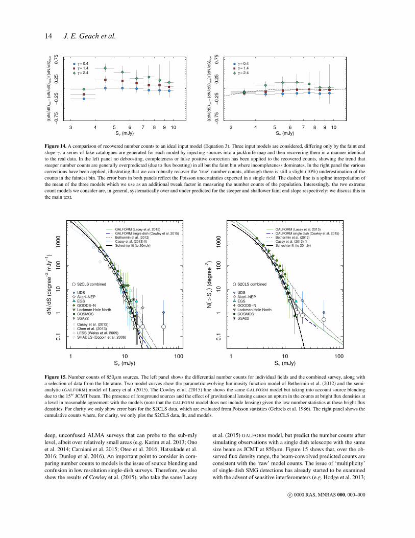
Figure 14. A comparison of recovered number counts to an ideal input model (Equation 3). Three input models are considered, differing only by the faint endslope γ: a series of fake catalogues are generated for each model by injecting sources into a jackknife map and then recovering them in a manner identicalto the real data. In the left panel no deboosting, completeness or false positive correction has been applied to the recovered counts, showing the trend thatsteeper number counts are generally overpredicted (due to flux boosting) in all but the faint bin where incompleteness dominates. In the right panel the variouscorrections have been applied, illustrating that we can robustly recover the ‘true’ number counts, although there is still a slight (10%) underestimation of thecounts in the faintest bin. The error bars in both panels reflect the Poisson uncertainties expected in a single field. The dashed line is a spline interpolation ofthe mean of the three models which we use as an additional tweak factor in measuring the number counts of the population. Interestingly, the two extremecount models we consider are, in general, systematically over and under predicted for the steeper and shallower faint end slope respectively; we discuss this inthe main text.

GALFORM (Lacey et al. 2015)

GALFORM single dish (Cowley et al. 2015)

Bethermin et al. (2012)

Casey et al. (2013) fit

Schechter fit (to 20mJy)

S2CLS combined


Casey et al. (2013)Chen et al. (2013)LESS (Weiss et al. 2009)SHADES (Coppin et al. 2006)

1 10 100

0.1

110

100

1000

Sν (mJy)

dN

dS

(degre

e−2 m

Jy

−1)

GALFORM (Lacey et al. 2015)

GALFORM single dish (Cowley et al. 2015)

Bethermin et al. (2012)

Casey et al. (2013) fit

Schechter fit (to 20mJy)

S2CLS combined


1 10 100

0.1

110

100

1000

Sν (mJy)

N(

>S

ν)

(degre

e−2)

Figure 15. Number counts of 850µm sources. The left panel shows the differential number counts for individual fields and the combined survey, along witha selection of data from the literature. Two model curves show the parametric evolving luminosity function model of Bethermin et al. (2012) and the semi-analytic (GALFORM) model of Lacey et al. (2015). The Cowley et al. (2015) line shows the same GALFORM model but taking into account source blendingdue to the 15′′ JCMT beam. The presence of foreground sources and the effect of gravitational lensing causes an upturn in the counts at bright flux densities ata level in reasonable agreement with the models (note that the GALFORM model does not include lensing) given the low number statistics at these bright fluxdensities. For clarity we only show error bars for the S2CLS data, which are evaluated from Poisson statistics (Gehrels et al. 1986). The right panel shows thecumulative counts where, for clarity, we only plot the S2CLS data, fit, and models.

deep, unconfused ALMA surveys that can probe to the sub-mJylevel, albeit over relatively small areas (e.g. Karim et al. 2013; Onoet al. 2014; Carniani et al. 2015; Oteo et al. 2016; Hatsukade et al.2016; Dunlop et al. 2016). An important point to consider in com-paring number counts to models is the issue of source blending andconfusion in low resolution single-dish surveys. Therefore, we alsoshow the results of Cowley et al. (2015), who take the same Lacey

et al. (2015) GALFORM model, but predict the number counts aftersimulating observations with a single dish telescope with the samesize beam as JCMT at 850µm. Figure 15 shows that, over the ob-served flux density range, the beam-convolved predicted counts areconsistent with the ‘raw’ model counts. The issue of ‘multiplicity’of single-dish SMG detections has already started to be examinedwith the advent of sensitive interferometers (e.g. Hodge et al. 2013;

c© 0000 RAS, MNRAS 000, 000–000


3 4 5 6 7 8 9 10

−1

01

23

Sν (mJy)

δ(

>S

ν)

=(ρ

−ρ)

ρ


Figure 16. Field-to-field scatter in the integral number counts, relative to themean density. The field-to-field scatter (on scales of 0.5–1) across S2CLSis generally within 50% of the mean density, with the exception of GOODS-N, which has hints of an elevated density of SMGs compared to the mean,although this is marginal with the Poisson uncertainties. We discuss this in§3.1.

Simpson et al. 2015), and it is important to stress that comparisonsof source abundances (between both models and data) should adopta consistent reference resolution.

While the semi-analytic models aim to simultaneously repro-duce all the main ‘bulk’ observational tracers of the galaxy pop-ulation over cosmic time (i.e. the mass function, luminosity func-tions, number counts, clustering, etc.) in a single framework, analternative approach to predicting the submillimetre number countsis through phenomenological modelling. Bethermin et al. (2012)present a model that considers the evolution of the space density ofso called ‘main sequence’ (i.e. normal) star-forming galaxies andluminous starbursts, fitting parametric models (with assumptionsabout the underlying galaxy SEDs) to observed number countsacross the infrared, submillimetre and radio bands. We show theBethermin et al. model (including the strong lensing contribution)for the SCUBA-2 850µm band in Figure 15. Again, this is in rea-sonable agreement with the observations over the flux range probedby the observations. The new 850µm number counts presented herecould be used to provide improved fits to phenomenological modelssuch as this.

4 SUMMARY

We have presented the 850µm maps and catalogues of the JamesClerk Maxwell Telescope SCUBA-2 Cosmology Legacy Survey,the largest of the JCMT Legacy Surveys, completed in early2015. With hundreds of hours of integration time in reasonablesubmillimetre observing conditions (zenith opacity τ225GHz =0.05–0.1) S2CLS has mapped seven well-known extragalactic sur-vey fields: UKIDSS-UDS, Akari-NEP, COSMOS, GOODS-N, Ex-tended Groth Strip, Lockman Hole North and SSA22. The total sci-entifically useful survey area is approximately 5 deg2 at a sensitiv-ity of under 2 mJy beam−1, with a median depth per field of approx-imately 1.2 mJy beam−1, approaching the confusion limit (whichwe have determined is approximately σc ≈ 0.8 mJy beam−1). Thisis by far the largest and deepest survey of submillimetre galaxiesyet undertaken in this waveband and provides a rich legacy data

source. We have detected nearly 3,000 submillimetre sources at the>3.5σ level, an order of magnitude increase in the number of cata-logued 850µm-selected sources to date.

In this work we have used the S2CLS catalogue to accuratelymeasure the number counts of submillimetre sources, dramaticallyreducing Poisson errors and allowing us to investigate field-to-fieldvariance. The wide nature of the survey makes it possible to de-tect large numbers of bright (>10 mJy), but rare (∼10 per squaredegree), submillimetre sources, and we observe the distinctive up-turn in the number counts caused by strong gravitational lensingof high redshift galaxies and a contribution from local sources ofsubmillimetre emission. The S2CLS catalogue and maps offer aroute to a tremendous range of follow-up work, both in pin-pointedmulti-wavelength identification and follow-up of the cataloguedsources (e.g. Simpson et al. 2015ab, Chen et al. 2016) and in sta-tistical analyses of the catalogues and pixel data. Cross-correlationof the submillimetre maps and galaxy catalogues is already prov-ing a treasure trove of discovery, linking UV/optical/near-infrared-selected samples to submillimetre emission (Banerji et al. 2015;Coppin et al. 2015; Smith et al. 2016 in preparation; Bourne et al.in preparation). The S2CLS survey subtends an area equivalent toover 105 times the ALMA primary beam at 850µm, and the syn-ergy between large area single dish surveys such as S2CLS, andthe detailed interferometric follow-up possible with ALMA (andother sensitive (sub)mm interferometers) is clear. High-resolutioninterferometric follow-up in the submillimetre has already provenefficient and fruitful, with ALMA and SMA imaging of the bright-est (>9 mJy) sources revealing a complex morphological mix, al-lowing us to investigate the true nature of the SMGs identified inlarge beam single dish surveys (Simpson et al. 2015, Chapman etal. in preparation). We release the 3.5σ-cut catalogue of all S2CLSsources as part of this publication, along with the 850µm maps forexploitation by the community. The data are available at the DOIhttp://dx.doi.org/10.5281/zenodo.57792

ACKNOWLEDGEMENTS

The authors thank M. Bethermin for supplying the SCUBA-2850µm number count predictions. The James Clerk Maxwell Tele-scope is now operated by the East Asian Observatory on behalf ofThe National Astronomical Observatory of Japan, Academia SinicaInstitute of Astronomy and Astrophysics, the Korea Astronomyand Space Science Institute, the National Astronomical Observa-tories of China and the Chinese Academy of Sciences (Grant No.XDB09000000), with additional funding support from the Scienceand Technology Facilities Council of the United Kingdom and par-ticipating universities in the United Kingdom and Canada. The datapresented in this paper was taken as part of Program ID MJLSC02.It is a pleasure to thank the entire staff of the JCMT for their superbsupport throughout the S2CLS campaign. Special thanks is due toIain Coulson, Jessica Dempsey, Jim Hoge, Harriet Parsons, CallieMatulonis, William Montgomerie and Holly Thomas. This researchused the facilities of the Canadian Astronomy Data Centre operatedby the National Research Council of Canada with the support of theCanadian Space Agency.

This work used the DiRAC Data Centric system at DurhamUniversity, operated by the Institute for Computational Cosmologyon behalf of the STFC DiRAC HPC Facility (www.dirac.ac.uk).This equipment was funded by BIS National E-infrastructure cap-ital grant ST/K00042X/1, STFC capital grant ST/H008519/1, and

c© 0000 RAS, MNRAS 000, 000–000


STFC DiRAC Operations grant ST/K003267/1 and Durham Uni-versity. DiRAC is part of the National E-Infrastructure.

JEG is supported by a Royal Society University Research Fel-lowship. IRS, AMS, JMS, ALRD, DMA, ACE and CGL acknowl-edge support from ST/L00075X/1. IRS also acknowledges supportfrom the ERC Advanced Grant DUSTYGAL (321334) and a RoyalSociety Wolfson Merit Award. JSD acknowledges the support ofthe European Research Council through the award of an AdvancedGrant. RJI acknowledges support from ERC in the form of the Ad-vanced Investigator Programme COSMICISM (321302). AK ac-knowledges support by the Collaborative Research Council 956,sub-project A1, funded by the Deutsche Forschungsgemeinschaft(DFG). KK acknowledges supports from the Swedish ResearchCouncil.

REFERENCES

Alaghband-Zadeh, S., Chapman, S. C., Swinbank, A. M., Smail, Ian, Har-rison, C. M., Alexander, D. M., Casey, C. M., Dav , R., et al. (2012),MNRAS, 424, 2232

Austermann, J. E., Dunlop, J. S., Perera, T. A., Scott, K. S., Wilson, G. W.,Aretxaga, I., Hughes, D. H., Almaini, O., et al. (2010) MNRAS, 401,160

Banerji, M., McMahon, R. G., Willott, C. J., Geach, J. E., Harrison, C.M., Alaghband-Zadeh, S., Alexander, D. M., Bourne, N., et al., (2015),MNRAS, 454, 419

Barger, A. J., Cowie, L. L., Sanders, D. B., Fulton, E., Taniguchi, Y., Sato,Y., Kawara, K., Okuda, H., (1998), Nature, 394, 248

Baugh, C. M., Lacey, C. G., Frenk, C. S., Granato, G. L., Silva, L., Bressan,A., Benson, A. J., Cole, S., (2005), MNRAS, 356, 1191

Be thermin, M., Daddi, E., Magdis, G., Sargent, M. T., Hezaveh, Y., Elbaz,D., Le Borgne, D., Mullaney, J., et al. (2012), ApJ, 757, 23

Blain, A. W., Longair, M. S., (1993), MNRAS, 264, 509Blain, A. W., Smail, Ian, Ivison, R. J., Kneib, J.-P., Frayer, D. T., (2002),

Physics Reports, 369, 2Borys, C., Chapman, S., Halpern, M., Scott, D., (2003), MNRAS, 344, 385Bothwell, M. S., Smail, Ian, Chapman, S. C., Genzel, R., Ivison, R. J., Tac-

coni, L. J., Alaghband-Zadeh, S., Bertoldi, F., et al. (2013), MNRAS,429, 3047

Carilli, C. L., Wang, Ran, Fan, X., Walter, F., Kurk, J., Riechers, D., Wagg,J., Hennawi, J., et al. (2010), ApJ, 714, 1407

Carniani, S., Maiolino, R., De Zotti, G., Negrello, M., Marconi, A., Both-well, M. S., Capak, P., Carilli, C., et al. (2015), A&A, 584, 78

Carlstrom, J. E., Ade, P. A. R., Aird, K. A., Benson, B. A., Bleem, L. E.,Busetti, S., Chang, C. L., Chauvin, E., et al., (2011), PASP, 123, 568

Casey, C. M., Chen, C-C., Cowie, L. L., Barger, A. J., Capak, P., Ilbert, O.,Koss, M., Lee, N., et al. (2013), MNRAS, 436, 1919

Chapin, E. L., Berry, D. S., Gibb, A. G., Jenness, T., Scott, D., Tilanus, R.P. J., Economou, F., Holland, W. S., (2013), MNRAS, 430, 2545

Chen, C-C., Smail, Ian, Ivison, R. J., Arumugam, V., Almaini, O., Con-selice, C. J., Geach, J. E., Hartley, W. G., et al. (2016), ApJ, 820, 82

Clements, D. L., Rowan-Robinson, M., Lawrence, A., Broadhurst, T.,McMahon, R., (1992), MNRAS, 256, 35

Condon, J. J., (1974), ApJ, 188, 279Coppin, K., Halpern, M., Scott, D., Borys, C., Chapman, S., (2005), MN-

RAS, 357, 1022Coppin, K., Chapin, E. L., Mortier, A. M. J., Scott, S. E., Borys, C., Dunlop,

J. S., Halpern, M., Hughes, D. H., et al. (2006), MNRAS, 372, 1621Coppin, K. E. K., Geach, J. E., Almaini, O., Arumugam, V., Dunlop, J. S.,

Hartley, W. G., Ivison, R. J., Simpson, C. J., et al. (2015), MNRAS,446, 1293

Cowley, W. I., Lacey, C. G., Baugh, C. M., Cole, S., (2015), MNRAS, 446,1784

Daddi, E., Dannerbauer, H., Stern, D., Dickinson, M., Morrison, G., Elbaz,D., Giavalisco, M., Mancini, C., et al. (2009), ApJ, 694, 1517

Day, P. K., LeDuc, H. G., Mazin, B. A., Vayonakis, A., Zmuidzinas, J.,(2003), Nature, 425, 817

Dempsey, J. T., Friberg, P., Jenness, T., Tilanus, R. P. J., Thomas, H. S.,Holland, W. S., Bintley, D., Berry, D. S., et al. (2013), MNRAS, 430,2534

Devlin, M. J., Ade, P. A. R., Aretxaga, I., Bock, J. J., Chapin, E. L., Griffin,M., Gundersen, J. O., Halpern, M., et al. (2009), Nature, 458, 737

Dole, H., Lagache, G., Puget, J. -L., Caputi, K. I., Fernandez-Conde, N., LeFloc’h, E., Papovich, C., P rez-Gonz lez, P. G., et al. (2006), A&A, 451,417

Duncan, W. D., Robson, E. I., Ade, P. A. R., Griffin, M. J., Sandell, G.,(1990), MNRAS, 243, 126

Eales, S., Dunne, L., Clements, D., Cooray, A., De Zotti, G., Dye, S., Ivison,R., Jarvis, M., et al. (2008), PASP, 122, 499

Engel, H., Tacconi, L. J., Davies, R. I., Neri, R., Smail, I., Chapman, S. C.,Genzel, R., Cox, P., et al. (2010) ApJ 724, 233

Fixsen, D. J., Dwek, E., Mather, J. C., Bennett, C. L., Shafer, R. A., (1998),ApJ, 508, 123

Geach, J. E., Chapin, E. L., Coppin, K. E. K., Dunlop, J. S., Halpern, M.,Smail, Ian, van der Werf, P., Serjeant, S., et al. (2013), MNRAS, 432,53

Genzel, R., Baker, A. J., Tacconi, L. J., Lutz, D., Cox, P., Guilloteau, S.,Omont, A., (2003), ApJ, 584, 633

Glenn, J., Bock, J. J., Chattopadhyay, G., Edgington, S. F., Lange, A. E.,Zmuidzinas, J., Mauskopf, P. D., Rownd, B., et al. (1998), Proc. SPIEVol. 3357, p. 326-334, Advanced Technology MMW, Radio, and Tera-hertz Telescopes, Thomas G. Phillips, Ed.

Greve, T. R., Ivison, R. J., Bertoldi, F., Stevens, J. A., Dunlop, J. S., Lutz,D., Carilli, C. L., (2004), MNRAS, 354, 779

Greve, T. R., Bertoldi, F., Smail, Ian, Neri, R., Chapman, S. C., Blain, A.W., Ivison, R. J., Genzel, R., et al. (2005), MNRAS, 359, 1165

Griffin, M., Swinyard, B., Vigroux, L., Abergel, A., Ade, P., Andre, P., Ba-luteau, J-P., Bock, J., et al., (2008), Space Telescopes and Instrumen-tation 2008: Optical, Infrared, and Millimeter. Edited by Oschmann,Jacobus M., Jr., de Graauw, Mattheus W. M., MacEwen, Howard A.Proceedings of the SPIE, Volume 7010, article id. 701006

Hainline, L. J., Blain, A. W., Smail, Ian, Alexander, D. M., Armus, L.,Chapman, S. C., Ivison, R. J., (2011), ApJ, 740, 96

Hayward, C. C., Behroozi, P. S., Somerville, R. S., Primack, J. R., Moreno,J., Wechsler, R. H., (2013), MNRAS, 434, 2572

Hildebrand, R., H, (1983), QJRAS, 24, 267Hodge, J. A., Karim, A., Smail, I., Swinbank, A. M., Walter, F., Biggs, A.

D., Ivison, R. J., Weiss, A., et al. (2013), ApJ, 768, 91Holland, W. S., Robson, E. I., Gear, W. K., Cunningham, C. R., Lightfoot,

J. F., Jenness, T., Ivison, R. J., Stevens, J. A., et al. (1999), MNRAS,303, 659

Holland, W. S., Bintley, D., Chapin, E. L., Chrysostomou, A., Davis, G. R.,Dempsey, J. T., Duncan, W. D., Fich, M., et al. (2013), MNRAS, 430,2513

Hughes, D. H., Serjeant, S., Dunlop, J., Rowan-Robinson, M., Blain, A.,Mann, R. G., Ivison, R., Peacock, J., (1998), Nature, 394, 241

Irwin, K. D., Hilton, G. C., (1995), Cryogenic Particle Detection, Topics inApplied Physics, Volume 99

Ivison, R. J., Greve, T. R., Dunlop, J. S., Peacock, J. A., Egami, E., Smail,Ian, Ibar, E., van Kampen, E., et al. (2007), MNRAS, 380, 199

Ivison, R. J., Smail, Ian, Amblard, A., Arumugam, V., De Breuck, C.,Emonts, B. H. C., Feain, I., Greve, T. R., et al. (2012), MNRAS, 425,1320

Jauncey, David L., (1968), ApJ, 152, 647Karim, A., Swinbank, A. M., Hodge, J. A., Smail, I. R., Walter, F., Biggs,

A. D., Simpson, J. M., Danielson, A. L. R., et al. (2013), MNRAS, 432,2

Knudsen, K. K., van der Werf, P. P., Kneib, J.P., (2008), MNRAS, 384, 1611Koprowski, M. P., Dunlop, J. S., Michalowski, M. J., Cirasuolo, M., Bowler,

R. A. A., (2014), MNRAS, 444, 117Lagos, C. del P., Bayet, E., Baugh, C. M., Lacey, C. G., Bell, T. A.,

Fanidakis, N., Geach, James E., (2012), MNRAS, 426, 2142Lehmer, B. D., Alexander, D. M., Chapman, S. C., Smail, Ian, Bauer, F. E.,

c© 0000 RAS, MNRAS 000, 000–000


Brandt, W. N., Geach, J. E., Matsuda, Y., et al. (2009), MNRAS, 400,299

Lilly, S. J., Eales, S. A., Gear, W. K. P., Hammer, F., Le Fevre, O., Cramp-ton, D., Bond, J. R., Dunne, L., (1999), ApJ, 518, 641

Magnelli, B., Lutz, D., Santini, P., Saintonge, A., Berta, S., Albrecht, M.,Altieri, B., Andreani, P., et al. (2012), A&A, 539, 155

Michalowski, M. J., Dunlop, J. S., Cirasuolo, M., Hjorth, J., Hayward, C.C., Watson, D., (2012), A&A, 541, 85

Monfardini, A., Swenson, L. J., Bideaud, A., D sert, F. X., Yates, S. J. C.,Benoit, A., Baryshev, A. M., Baselmans, J. J. A., et al. (2010), A&A,521, 29

Narayanan, D., Turk, M., Feldmann, R., Robitaille, T., Hopkins, P., Thomp-son, R., Hayward, C., Ball, D., et al. (2015), Nature, 525, 496

Negrello, M., Hopwood, R., De Zotti, G., Cooray, A., Verma, A., Bock, J.,Frayer, D. T., Gurwell, M. A., et al. (2010), Science, 330, 800

Ono, Y., Ouchi, M., Kurono, Y., Momose, R., (2014), ApJ, 795, 5Oteo, I., Zwaan, M. A., Ivison, R. J., Smail, I., Biggs, A. D., (2016), ApJ,

822, 36Padoan, P., Nordlund, øA, (2002), ApJ, 576, 870Pascale, E., Ade, P. A. R., Bock, J. J., Chapin, E. L., Chung, J., Devlin, M.

J., Dicker, S., Griffin, M., et al. (2008), ApJ, 681, 400Pope, A., Borys, C., Scott, D., Conselice, C., Dickinson, M., Mobasher, B.,

(2005), MNRAS, 358, 149Puget, J. -L., Abergel, A., Bernard, J. -P., Boulanger, F., Burton, W. B.,

Desert, F. -X., Hartmann, D., (1996), A&A, 308, 5Rowan-Robinson, M., Broadhurst, T., Lawrence, A., McMahon, R. G.,

Lonsdale, C. J., Oliver, S. J., Taylor, A. N., Hacking, P. B., et al. (1991),Nature, 351, 719

Sanders, D. B., Salvato, M., Aussel, H., Ilbert, O., Scoville, N., Surace, J.A., Frayer, D. T., Sheth, K., et al. (2007), ApJS, 172, 86

Scott, S. E., Dunlop, J. S., Serjeant, S., (2006), MNRAS, 370, 1057Simpson, J. M., Smail, Ian, Swinbank, A. M., Chapman, S. C., Geach, J. E.,

Ivison, R. J., Thomson, A. P., Aretxaga, I., et al. (2015), ApJ, 807, 128Siringo, G., Kreysa, E., Kovacs, A., Schuller, F., Weiss, A., Esch, W.,

Gemund, H.-P., Jethava, N., et al. (2009), A&A, 497, 945Smail, Ian, Ivison, R. J., Blain, A. W., (1997), ApJ, 490, 5Somerville, R. S., Moustakas, L. A., Mobasher, B., Gardner, J. P., Cimatti,

A., Conselice, C., Daddi, E., Dahlen, T., et al. (2004), ApJ, 600, 171Swetz, D. S., Ade, P. A. R., Amiri, M., Appel, J. W., Battistelli, E. S.,

Burger, B., Chervenak, J., Devlin, M. J., et al., (2011), ApJS, 194, 41Swinbank, A. M., Smail, Ian, Chapman, S. C., Blain, A. W., Ivison, R. J.,

Keel, W. C., (2004), ApJ, 617, 64Swinbank, A. M., Chapman, S. C., Smail, Ian, Lindner, C., Borys, C., Blain,

A. W., Ivison, R. J., Lewis, G. F., (2006), MNRAS 371, 465Swinbank, A. M., Smail, Ian, Chapman, S. C., Borys, C., Alexander, D. M.,

Blain, A. W., Conselice, C. J., Hainline, L. J., et al. (2010), MNRAS,405, 234

Swinbank, A. M., Simpson, J. M., Smail, Ian, Harrison, C. M., Hodge, J. A.,Karim, A., Walter, F., Alexander, D. M., et al. (2014), MNRAS, 438,1267

Tacconi, L. J., Neri, R., Chapman, S. C., Genzel, R., Smail, I., Ivison, R. J.,Bertoldi, F., Blain, A., et al. (2006), ApJ, 640 ,228

Tacconi, L. J., Genzel, R., Smail, I., Neri, R., Chapman, S. C., Ivison, R. J.,Blain, A., Cox, P., et al. (2008), ApJ, 680, 246

Tacconi, L. J., Genzel, R., Neri, R., Cox, P., Cooper, M. C., Shapiro, K.,Bolatto, A., Bouch , N., et al. (2010), Nature, 463, 781

Targett, T. A., Dunlop, J. S., Cirasuolo, M., McLure, R. J., Bruce, V. A.,Fontana, A., Galametz, A., Paris, D., et al. (2013) MNRAS, 432, 2012

Trenti, M., Stiavelli, M., (2008), ApJ, 676, 767Walter, F., Decarli, R., Carilli, C., Bertoldi, F., Cox, P., da Cunha, E., Daddi,

E., Dickinson, M., et al., (2009), Nature, 486, 233Wardlow, J. L., Smail, Ian, Coppin, K. E. K., Alexander, D. M., Brandt,

W. N., Danielson, A. L. R., Luo, B., Swinbank, A. M., et al. (2011)MNRAS, 415, 1479

Wang, N., Hunter, T. R., Benford, D. J., Serabyn, E., Lis, D. C., Phillips, T.G., Moseley, S. H., Boyce, K., et al. (1996), Applied Optics, 35, 34

Wilson, G. W., Austermann, J. E., Perera, T. A., Scott, K. S., Ade, P. A. R.,Bock, J. J., Glenn, J., Golwala, S. R., et al. (2008), MNRAS, 386, 807

c© 0000 RAS, MNRAS 000, 000–000


2 Institute for Astronomy, University of Edinburgh, Royal Observatory, Blackford Hill, Edinburgh, EH9 3HJ3 Department of Physics & Astronomy, University of British Columbia, 6224 Agricultural Road, Vancouver, BC, V6T 1Z1, Canada4 Centre for Extragalactic Astronomy, Department of Physics, Durham University, South Road, Durham, DH1 3LE5 Leiden Observatory, Leiden University, P.O. box 9513, 2300 RA Leiden, The Netherlands6 School of Physics and Astronomy, University of Nottingham, University Park, Nottingham, NG9 2RD7 Instituto Nacional de Astrofısica Optica y Electronica, Calle Luis Enrique Erro No. 1, Sta. Ma. Tonantzintla, Puebla, Mexico8 European Southern Observatory, Karl-Schwarzschild-Str. 2, D-85748 Garching, Germany9 Institute of Astronomy, University of Cambridge, Madingley Road, Cambridge, CB3 OHA10 Department of Astronomy & Physics, St Mary’s University, 923 Robie St., Halifax, Nova Scotia, B3H 3C3, Canada11 Department of Physics & Astronomy, University of Leicester, University Road, Leicester, LE1 7RH12 H. H. Wills Physics Laboratory, University of Bristol, Tyndall Avenue, Bristol, BS8 1TL13 Herzberg Astronomy and Astrophysics, National Research Council Canada, 5071 West Saanich Road, Victoria, BC V9E 2E7, Canada14 Department of Physics and Atmospheric Science, Dalhousie University Halifax, NS, B3H 3J5, Canada15 SKA Headquarters, The University of Manchester, Manchester, M13 9PL16 Astronomy Centre, Department of Physics and Astronomy, University of Sussex, Brighton, BN1 9QH17 Astrophysics Group, Imperial College London, Blackett Laboratory, Prince Consort Road, London, SW7 2AZ18 Institute for Computational Cosmology, Department of Physics, Durham University, South Road, Durham, DH1 3LE19 School of Physics and Astronomy, Cardiff University, Queen’s Buildings, The Parade, Cardiff, CF24 3AA20 Virginia Polytechnic Institute & State University Department of Physics, MC 0435, 910 Drillfield Drive, Blacksburg, VA 24061, USA21 Department of Physics, University of Oxford, Keble Road, Oxford, OX1 3RH22 Department of Physics, University of the Western Cape, Bellville 7535, South Africa23 Department of Earth and Space Science, Chalmers University of Technology, Onsala Space Observatory, SE-43992 Onsala, Sweden24 Argelander-Institut fur Astronomie, Universitat Bonn, Auf dem Hugel 71, D-53121 Bonn, Germany25 Kapteyn Institute, University of Groningen, P.O. Box 800, 9700 AV Groningen, The Netherlands26 Mullard Space Science Laboratory, University College London, Holmbury St Mary Dorking, Surrey, RH5 6NT27 Space Science & Technology Department, Rutherford Appleton Laboratory, Chilton, Didcot, Oxfordshire, OX11 0QX28 UK Astronomy Technology Centre, Royal Observatory, Blackford Hill, Edinburgh, EH9 3HJ29 Robert Hooke Building, Department of Physical Sciences, The Open University, Milton Keynes, MK7 6AA30 Gemini Observatory, Northern Operations Center, 760 N. A‘ohoku Place, Hilo, HI 96720, USA31 Department of Physics and Astronomy, Sonoma State University, 1801 East Cotati Avenue, Rohnert Park, CA 94928-3609, USA32 Department of Physics, McGill University, 3600 rue University, Montreal, QC H3A 2T8, Canada33 Canadian Astronomy Data Centre, National Research Council Canada, 5071 West Saanich Road, Victoria, BC, V9E 2E7, Canada34 Center for Detectors, School of Physics and Astronomy, Rochester Institute of Technology, Rochester, NY 14623, USA35 Jet Propulsion Laboratory, 4800 Oak Grove Drive, Pasadena, CA 91109, USA

c© 0000 RAS, MNRAS 000, 000–000

The SCUBA-2 Cosmology Legacy Survey: 850 and number counts

Documents