The scars of youth - IAB

IAB Discussion PaperArticles on labour market issues

6/2013

Achim Schmillen Matthias Umkehrer

ISSN 2195-2663

The scars of youthEffects of early-career unemployment on future unemployment experience

The Scars of Youth — Effects of Early-Career

Unemployment on Future Unemployment

Experience

Achim Schmillen (IAB, National Bureau of Economic Research, Institute for East

and Southeast European Studies)

Matthias Umkehrer (IAB)

Mit der Reihe „IAB-Discussion Paper“ will das Forschungsinstitut der Bundesagentur für Arbeit den

Dialog mit der externen Wissenschaft intensivieren. Durch die rasche Verbreitung von Forschungs-

ergebnissen über das Internet soll noch vor Drucklegung Kritik angeregt und Qualität gesichert

werden.

The “IAB Discussion Paper” is published by the research institute of the German Federal Employ-

ment Agency in order to intensify the dialogue with the scientific community. The prompt publication

of the latest research results via the internet intends to stimulate criticism and to ensure research

quality at an early stage before printing.

IAB-Discussion Paper 6/2013 2

Contents

Abstract . . . . . . . . . . . . . . . . . . . . . . . . . . . . . . . . . . . . . . . 4

Zusammenfassung . . . . . . . . . . . . . . . . . . . . . . . . . . . . . . . . . . 4

1 Introduction . . . . . . . . . . . . . . . . . . . . . . . . . . . . . . . . . . . . 5

2 Conceptual Considerations . . . . . . . . . . . . . . . . . . . . . . . . . . . . 7

3 Data . . . . . . . . . . . . . . . . . . . . . . . . . . . . . . . . . . . . . . . 11

4 Unemployment Dynamics During the Professional Career . . . . . . . . . . . . 13

5 Scarring Effects of Youth Unemployment . . . . . . . . . . . . . . . . . . . . . 155.1 Baseline Estimates . . . . . . . . . . . . . . . . . . . . . . . . . . . . . 155.2 Sensitivity and Specification Tests . . . . . . . . . . . . . . . . . . . . . 195.3 Interpreting the Regression Results . . . . . . . . . . . . . . . . . . . . . 24

6 Heterogeneity in Scarring Effects . . . . . . . . . . . . . . . . . . . . . . . . . 26

7 Conclusions . . . . . . . . . . . . . . . . . . . . . . . . . . . . . . . . . . . 30

References . . . . . . . . . . . . . . . . . . . . . . . . . . . . . . . . . . . . . . 32

8 Appendix . . . . . . . . . . . . . . . . . . . . . . . . . . . . . . . . . . . . . 378.1 Data Selection, Control Variables and Summary Statistics . . . . . . . . . 378.2 Early-Career Unemployment and Different Outcomes in Prime Age . . . . . 388.3 Adjustment Processes and Short-run Unemployment Dynamics . . . . . . 418.4 Local Average Treatment Effects and Average Causal Effects . . . . . . . . 438.5 Censored Quantile Instrumental Variable Regression . . . . . . . . . . . . 478.6 Supplementary Tables and Figures . . . . . . . . . . . . . . . . . . . . . 50


Abstract

Does early-career unemployment cause future unemployment? We answer this ques-

tion with German administrative matched employer-employee data that track more than

800,000 individuals over 24 years. Using a censored quantile instrumental variable esti-

mator and instrumenting early-career unemployment with local labor market conditions at

labor market entry and firm-specific labor demand shocks, we find significant and long-

lasting scarring effects. At the median, an additional day of unemployment during the first

eight years on the labor market increases unemployment in the following 16 years by 0.96

days. Effects are even stronger in the right tail of the unemployment distribution. Likely

due to unobserved heterogeneity in returns to search, they are also understated by non-IV

estimates.

Zusammenfassung

Steht Jugendarbeitslosigkeit in einem kausalen Zusammenhang mit der Erfahrung spä-

terer Arbeitslosigkeit? Wir beantworten diese Frage mit Hilfe administrativer Integrierter

Betriebs- und Personendaten, welche es uns erlauben, mehr als 800.000 Personen über

24 Jahre hinweg zu folgen. Indem wir Jugendarbeitslosigkeit durch zum Zeitpunkt des

Arbeitsmarkteintritts vorherrschende regionale Arbeitsmarktbedingungen und firmenspezi-

fische Arbeitsnachfrageschocks instrumentieren und Zensierte-Instrumentvariablen-Quan-

tilsregressionen heranziehen, zeigen wir, dass Jugendarbeitslosigkeit signifikante und lang

anhaltende “Scarring”-Effekte nach sich zieht. Im Median führt ein zusätzlicher Tag Ju-

gendarbeitslosigkeit zu 0,96 weiteren Tagen Arbeitslosigkeit während der späteren Erwerb-

sphase. Im oberen Bereich der Arbeitslosigkeitsverteilung sind die Effekte noch ausge-

prägter.

JEL classification: J64, J62, C20

Keywords: Scarring; state dependence; censored quantile instrumental variable re-

gressions

Acknowledgements: We would like to thank Joachim Möller, Joshua Angrist, Stefan

Bender, Philipp vom Berge, David Card, Bernd Fitzenberger, Hans-Jörg Schmerer,

Michael Stops and Mariana Viollaz as well as conference and seminar participants

in Bayreuth, Bonn, Boston, Freiburg, Göttingen, Kallmünz, Malaga, Mannheim and

Nuremberg for helpful comments and suggestions. The usual disclaimer applies.


1 Introduction

Two conflicting notions of early-career unemployment are to be found in the literature: one

contends that during the first years on the labor market an adjustment process takes place

where job shopping enables individuals to offset disadvantageous initial conditions, gather

heterogeneous experiences and find their place in the professional world [cf. Freeman

and Wise (1982) or Topel and Ward (1992)]. From this viewpoint, an elevated amount of

youth unemployment could be seen as nothing more than a temporary nuisance and any

observed persistence in unemployment would be due to temporally correlated individual

differences in the probability of experiencing unemployment. If, by contrast, early-career

unemployment delayed the accumulation of productive skills and knowledge or prevented

the formation of tight employer-employee matches, the picture would change dramatically:

unemployment, in particular, might then exhibit true state dependence, i.e. unemployment

early in the professional career might causally lead to more unemployment later in life.1

Ultimately, the question whether early-career unemployment causes future unemployment

can only be answered empirically. This is exactly what our study aims to achieve. With the

help of German administrative matched employer-employee data we detail the dynamics

of unemployment during a professional career, documenting that unemployment is highly

persistent amongst a group of individuals. Even though we find some evidence that youth

unemployment may partly be a side effect of early-career adjustment processes, we reach

the conclusion that its persistence is due to true state dependence (at least to a large

extent): On average, every day of unemployment during the first eight years of the pro-

fessional career induces two additional days of unemployment during the subsequent 16

years, all else being equal. OLS estimates in fact understate this scarring effect of youth

unemployment, arguably because of unobserved heterogeneity in individuals’ returns to

search. Scarring also varies considerably across the (conditional) distribution of prime-age

unemployment and is strongest in its right tail. While at the median an additional day of

youth unemployment leads to an increase in prime-age unemployment of less than one

day, at the 95th percentile another day of early-career unemployment induces almost six

and a half days of prime-age unemployment, ceteris paribus. These high numbers imply

that the long-term scarring effect of youth unemployment is not only statistically significant

but also economically important.

We base our analysis on an administrative matched employer-employee data set that con-

tains the universe of social security records in Germany. From these, we extract the com-

plete employment biographies of all 827,114 men who graduated from Germany’s dual

education system between 1978 and 1980.2 This system combines apprenticeships in a

company and vocational education at a school in one course. In our view, it is an ideal in-

stitutional environment to study the effects of early-career unemployment. That is because

the majority (around 60 percent) of young people enter the German labor market through

the dual education system, because apprentices constitute a fairly homogeneous group in

1 If “unemployment (...) alters preferences, prices or constraints that determine, in part, future unemploy-ment”, Heckman and Borjas (1980: p. 247) call this true state dependence.

2 We concentrate on men because data problems make an analysis for women conceptually difficult [cf.Appendix 8.1].


regard to their experience, training and background and because by focusing on its grad-

uates we avoid for the most part any problems caused by unobserved initial conditions

[cf. Hoffmann (2010)].

Our data make it possible to identify the exact time and place of labor market entry for all

827,114 individuals and to track them for every day of the first 24 years of their profes-

sional careers. Instead of relying on a traditional analysis of distinct unemployment spells

focusing on durations or Markov transition rates, we examine whether an individual’s to-

tal amount of unemployment during the eight years after graduation influences the overall

length of unemployment spells in the subsequent 16 years. Compared to a period-to-period

approach, this strategy is better able to capture medium- and long-run scarring effects of

youth unemployment. It also provides more suitable measures of long-term labor market

“success” or “failure”.

A large proportion of individuals in our sample experiences only short periods of unem-

ployment during their professional career or none at all. Others suffer from repeated and

prolonged periods of joblessness. That is why estimations of the conditional mean func-

tion may leave unrevealed important aspects of the relationship between early-career and

prime-age unemployment. Consequently, we make use of the innovative censored quan-

tile instrumental variable (CQIV) estimator introduced by Chernozhukov, Fernández-Val

and Kowalski (2011). This estimator not only takes into account the potential endogeneity

of early-career unemployment as well as the fact that almost 60 percent of the individuals in

our sample experience no prime-age unemployment at all but also allows marginal effects

to vary over the conditional distribution of prime-age unemployment. It thus identifies the

marginal quantiles of potential outcomes that, as Chernozhukov and Hansen (2005) argue,

are typically relevant for welfare analyses.

We instrument youth unemployment with local labor market conditions at labor market entry

and firm-specific labor demand shocks. Drawing on Gregg (2001), the first instrument

we use is the local unemployment rate right before graduation from the dual education

system. We consider this instrument to be relevant because it influences the quality of

initial matching of graduates to firms, ignorably assigned because the choice of location at

labor market entry can be assumed to be exogenous given location-specific fixed effects

and excluded because time-varying patterns of economic conditions, the accumulation of

skills and early matching processes prevent it from influencing prime-age unemployment

through channels other than youth unemployment. Our second instrument is a dummy

variable for whether an individual’s training firm closes in the year of his graduation. This is

a suitable instrument, too, because such plant closures induce a period of job search often

accompanied by unemployment, are almost impossible to predict and reflect a transitory

labor demand shock. Ultimately, the IV strategy exploits exogenous variation in initial labor

market conditions on the level of the local labor market and of the establishment and allows

us to do more than simply show that unemployment is highly persistent amongst a group

of individuals: we argue that we capture a causal relationship.

This study contributes to the broader literature on true state dependence [partly surveyed

in Ryan (2001)]. Early work by Heckman and Borjas (1980), Ellwood (1982) and Corcoran


and Hill (1985) finds little evidence of scarring in American data. A more recent study for the

United States by Mroz and Savage (2006) documents permanent wage losses due to early

unemployment experience but no significant unemployment effects. European research

usually finds stronger evidence in favor of state dependence: results by Nilsen and Reiso

(2011) and Nordström Skans (2011) suggest that it exists for Norway, and Arulampalam,

Booth and Taylor (2000), Arulampalam (2001), Gregg (2001), and Gregg and Tominey

(2005) find the same for Great Britain [Burgess, Propper, Rees and Shearer (2003) report

negative effects of early-career unemployment only for the unskilled but slightly positive

effects for skilled individuals]. Concerning Germany, very little is known about the scarring

effects of youth unemployment. The few relevant studies — most prominently Mühleisen

and Zimmermann (1994), Schmelzer (2010), and Niedergesäss (2012) — tend to address

state dependence more generally and universally confirm its existence.

More generally, we aim to contribute to the literature on long-term effects of labor market

events or decisions early in the professional career.3 von Wachter and Bender (2006), in

particular, also rely on German administrative matched employer-employee data and an

instrumental variable approach. Their research question is quite different, though: von

Wachter and Bender (2006) are concerned with the long-term effects of having to leave the

training firm after graduation from the dual education system. Thus, they are concerned

with the initial transition from training to the labor market. We complement their analysis by

focusing not on this transition but on the subsequent phase of the professional career. In

any case, their conclusion that at least for some groups of young workers having to leave

the training firm leads to persistent wage losses while for others losses are non-negligible

but drop to zero within five years is entirely consistent with our findings.

The remainder of this paper is structured as follows: conceptual considerations are dis-

cussed in the next section followed by a brief description of our matched employer-employee

data set. In Section 4, we characterize unemployment dynamics over the professional ca-

reer. Section 5 contains the findings of our main multivariate analysis, discusses their

robustness in regard to variations of the empirical setup and interprets the non-IV versus

the IV results. Digging deeper, Section 6 investigates how scarring varies over different

phases of the professional career and different quantiles of the (conditional) distribution of

prime-age unemployment. Finally, Section 7 concludes.

2 Conceptual Considerations

Theoretical explanations of scarring usually rely on one of the following three mechanisms:

first, in many search and matching frameworks, unemployed individuals lower their reser-

vation wages over time. As shown by Mortensen (1986), this behavior could on the one

hand shorten the duration of unemployment periods. On the other hand, however, it could

3 Examples include Raaum and Røed (2006), Stevens (2008) and Oreopoulos, von Wachter and Heisz(2012), who show that business cycle conditions at the time of labor market entry have economically signif-icant and long-lasting wage and employment effects and the more structurally oriented literature on careerdynamics, like Keane and Wolpin (1997) or Hoffmann (2010).


also mean that long-term unemployed individuals accept jobs that are not really a suitable

match. They could then be more likely to become unemployed again in the future.

Second, models by Pissarides (1992), Acemoglu (1995) and others stress the importance

of human capital. They conjecture that valuable skills and/or knowledge depreciate dur-

ing unemployment. Indeed, Edin and Gustavsson (2008) show that in Sweden one year

of nonemployment is associated on average with a five-percentile move down the skill

distribution. Such loss of human capital lowers an individual’s productivity and leads to

persistently lower earnings and a higher risk of experiencing unemployment. Youth un-

employment might be particularly harmful because the greatest investments in learning

are usually made at the beginning of one’s professional career [cf. Ben-Porath’s (1967)

life-cycle human capital model]. Moreover, for young people the lack of work experience

during unemployment might mean that crucial skills are never even acquired.

Third, if employers are unable to perfectly observe applicants’ productivity when making

hiring decisions, they may use previous unemployment spells as a screening device. They

may thus prefer to hire workers with less unemployment experience. Such stigma effects of

unemployment are prominently incorporated into the models of Vishwanath (1989), Lock-

wood (1991), Gibbons and Katz (1991) and Kroft, Lange and Notowidigdo (forthcoming).

Empirically, Gibbons and Katz (1991) find that the wage and employment consequences

of job displacement appear to be at least partly due to stigma effects.4, 5

Against this backdrop, we test whether there is a causal link between early-career unem-

ployment and long-term labor market outcomes with the help of the following econometric

model of prime-age unemployment:

m∗i,c,t2 = c+ αmi,c,t1 + x′i,c,t0β + µi + ρi + ηr + νc + ui,c,t2, (1)

where subscript c = {1978, 1979, 1980} denotes the labor market entry cohort, subscript

i = {1, ..., N} the individual, and subscript r = {1, ..., R} the district of the training firm.

t = {t0, t1, t2} indicates whether a variable is measured prior to labor market entry, early in

the professional career, or during prime age, respectively. Prime-age unemployment (m∗t2)

is the dependent variable while regressors include a vector of control variables (xt0) and a

constant (c). All control variables (graduation age, daily remuneration, occupation, sector,

size, and median wage of the training firm) are measured before labor market entry and

can arguably be considered exogenous. Besides, prime-age unemployment is determined

by effects specific to the individual’s ability (µi), job search behavior (ρi), and labor market

entry cohort (νc), as well as the training firm’s district (ηr) and an i.i.d. error term (ut2).

The pivotal explanatory variable is unemployment early in the professional career (mt1). If

4 Recent research by Kroft, Lange and Notowidigdo (forthcoming) suggests that actual employer behaviortoward unemployed job applicants might be more easily explained by stigma effects of unemployment ratherthan by a depreciation of their human capital [see also Cockx and Picchio (forthcoming)].

5 There is a plethora of alternative explanations for the existence of state dependence. Underlying factorsmentioned in the literature include contracts [Beaudry and diNardo (1991)], labor unions, hiring and firingcosts, discouragement or habituation effects [Clark, Georgellis and Sanfey (2001)], the lack of physicalcapital after recessions or the different bargaining powers of insiders and outsiders; cf. Margolis, Simonnetand Vilhuber (2001) for an overview.


this variable is measured with error et1, we only observe mt1 = mt1 + et1. Equation (1)

then becomes:

m∗i,c,t2 = c+ αmi,c,t1 − αei,c,t1 + x′i,c,t0β + µi + ρi + ηr + νc + ui,c,t2. (2)

Ultimately, we are interested in estimating the size of α. As we observe neither mt1, µi,

ρi, ηr nor νc directly, the probability limit of α from estimating equation (2) by ordinary least

squares (and suppressing νc) is given by

plim αols = α(1− cov(ei,c,t1, mi,c,t1)

var(mi,c,t1))+

cov(µi, mi,c,t1)

var(mi,c,t1)+cov(ρi, mi,c,t1)

var(mi,c,t1)+cov(ηr, mi,c,t1)

var(mi,c,t1).

(3)

Can we say anything about the likely direction of the bias? The first term on the right-hand

side of equation (3), α(1− cov(et1,mt1)var(mt1)

), refers to potential measurement error in the latent

amount of early-career unemployment. Under classical assumptions this attenuates simple

estimates of α toward zero [cf. Hausman (2001)]. It would thus lead OLS to understate the

scarring effect of early-career unemployment. The second term, cov(µ,mt1)var(mt1), represents abil-

ity bias. Omitting information on unobserved individual skills or motivation would upwardly

bias simple OLS estimates of α if ability were negatively correlated with the total durations

of both prime-age and early-career unemployment. At first glance, this might appear plau-

sible. Yet, unobserved ability might also induce a positive correlation between µ and mt1,

introducing a downward bias instead. As pointed out by Neumark (2002), this might for

instance be the case if the returns to job shopping were positively correlated with ability or

if the returns to job search rose faster with ability as compared to the costs of search.

The third term on the right-hand side of equation (3), cov(ρ,mt1)var(mt1), constitutes potential bias

resulting from unobserved differences in individuals’ job search behavior (orthogonal to

unobserved ability). If the returns to job hopping and/or the returns to search were consid-

erably higher for a certain group of individuals, members of this group would be expected

to spend more time searching for or switching jobs early in their professional careers. This

might extend the time they are unemployed during the first years on the labor market. But,

ultimately, it might also mean that they tend to be more successful with their search ef-

forts, eventually reaching more stable matches and lower prime-age unemployment. Such

a mechanism would generate a positive correlation between ρ and mt1 in equation (3). It

would therefore contribute to downward-biased OLS estimates [cf. Neumark (2002)].

Because of the term cov(η,mt1)var(mt1)

(which can be interpreted as reflecting initial sorting of in-

dividuals), not controlling for location-specific fixed effects would similarly induce a bias in

OLS or even simple IV estimates of α. If cov(η, mt1) > 0, it would lead to a downward

bias, and if cov(η, mt1) < 0, to an upward bias.

Because of these diverse sources of bias with sometimes ambiguous direction we pursue

an identification strategy where we will sequentially remove one source of bias after the

other. We will begin with a simple OLS estimation that will already control for quite a

number of socio-demographic and firm-related variables. Next, we will draw on Heckman

and Borjas (1980), as well as Gregg (2001) and Neumark (2002) and will instrument early-


career unemployment with local labor market conditions prevailing at the training firm’s

location right before graduation.6 If the identifying assumptions hold, this approach should

rid our estimates of α of any biases from measurement error, unobserved ability, or job

search behavior. Finally, to ensure that the instrument is as good as randomly assigned,

we will control for initial sorting of individuals by including fixed effects for the training firms’

districts.

Our main instrument will be the local unemployment rate right before graduation, where

locations will be defined by the administrative districts of Germany’s Federal Employment

Agency. We can distinguish 141 such functional labor market units with unemployment

rates varying considerably from 0.9 (the district of Nagold in 1979) to 8.2 percent (the

district of Saarbrücken in 1978). In our view the local unemployment rate at graduation is

a suitable instrument because it is relevant, ignorably assigned and excluded.

The instrument is relevant because the conditions that prevail just before labor market en-

try have an effect on whether an individual becomes unemployed after graduation from the

dual education system and, if this is the case, on the duration of the resulting unemploy-

ment spell. In fact, Raaum and Røed (2006) use Norwegian data to show that individuals

entering the labor market have greater difficulty establishing themselves on this market if

local unemployment rates are high. Besides, conditions at labor market entry affect the

quality of initial matching of apprentices to firms [cf. Bowlus (1995)]. In turn, the quality of

the initial match is important for early-career employment stability, adjustment processes

and, in particular, early-career unemployment.

We consider the instrument to be ignorably assigned since, following Gregg’s (2001) rea-

soning, the choice of location at labor market entry can be assumed to be exogenous. In

our sample, individuals are on average younger than 17 when they begin training. At this

age, most individuals still live with their parents and do not have the means to move to

another region. Indeed, we observe that 97.6 percent of individuals in our sample do not

change district during their apprenticeship.7 Still, there may be some sorting of individuals

into certain districts before the start of the apprenticeship (in Germany it is not uncommon

for apprentices to live in assigned boarding houses which might be located relatively far

away from their original place of residence, for instance). Alternatively, sorting might occur

even earlier by the individuals’ parents. To be on the safe side, we exploit the repeated

cross-sectional design of our data set and control for geographical sorting by including

fixed effects for the training firms’ districts.

We argue that the instrument is excluded because time-varying patterns of economic con-

ditions, the accumulation of skills, and the dynamism of matching processes early in the

professional career prevent it from influencing prime-age unemployment through channels

6 Local labor market conditions will be captured on June 30th of the graduation year if the apprenticeship iscompleted on or after that day, and on June 30th of the year prior to graduation if the graduation takes placeearlier.

7 35.7 percent of graduates do not stay at their training firm after graduation. Of these, 40 percent changedistrict between graduation and their first job subject to social security contributions. So the location of thefirst employment or unemployment spell has to be considered endogenous. This is why our identificationstrategy relies on the local labor market conditions right before graduation.


other than youth unemployment. In any case, we follow Gregg (2001) and control for local

unemployment rates eight years after graduation, thereby hoping to capture any possible

correlations due to persistent local labor market patterns.8

Finally, a regression of prime-age unemployment on early-career unemployment poses a

somewhat more technical challenge: as will be shown in Section 4, nearly 60 percent of

the individuals in our sample were not unemployed for a single day during prime age. Thus

we are faced with the typical case of censoring or rather a corner solution outcome as

defined by Wooldridge (2002). As a consequence, OLS or even simple IV estimates would

be biased and inconsistent because of a correlation between the regressors and the error

term. Accordingly, we interpret m∗t2 as the latent amount of prime-age unemployment as

opposed to the amount of prime-age unemployment actually observed, mt2. It holds that

mi,t2 =

m∗i,t2 if m∗i,t2 ≥ 0 and

0 if m∗i,t2 < 0.(4)

To address the issue of a corner solution outcome in practice, we supplement our OLS

regressions by simple Tobit models [cf. Tobin (1958)]. Correspondingly, all estimations

involving instruments are done with both the standard IV estimator and Smith and Blun-

dell’s (1986) conditional maximum likelihood estimator for a Tobit model with continuous

endogenous regressors. Similarly, when addressing the issue of heterogeneity of scarring

effects, we account for the corner solution by resorting to censored quantile and censored

quantile instrumental variable estimators.

3 Data

We rely on matched employer-employee data created by merging two data sets: first, the

Integrated Employment Biographies [IEB, cf. Oberschachtsiek, Scioch, Seysen and Hein-

ing (2009)] and, second, the Establishment History Panel (BHP). Both are administrative

data sets provided by the Institute for Employment Research in Nuremberg, Germany.

The IEB contain the universe of all individuals who received unemployment benefits and/or

were employed subject to social security contributions in the Federal Republic of Germany

at least once between 1975 and 2008. Only spells of employment not covered by social

security — like those of civil servants or family workers — and spells of self-employment

are not included in the data. All in all, the IEB cover about 80 percent of Germany’s total

workforce and encompass detailed longitudinal information on employment status, wages,

socio-demographic and firm characteristics to the exact day. Because Germany’s social

security agencies use the underlying administrative data to compute social security contri-

butions and unemployment benefits, they are highly reliable. In the context of our study,

8 Our empirical approach does not allow us to use individual-specific fixed effects. However, as mentionedabove and documented in Section 4, the early years of the professional career are often seen as providingopportunities for adjustments and for finding a productive employer-employee match. As also argued byvon Wachter and Bender (2006), in the context of the youth labor market controlling for unobserved time-invariant individual heterogeneity would be of little use.


another important advantage of not relying on survey but on administrative data is that we

need not worry about panel mortality or non-response.

For the purposes of this study, the IEB are matched with establishment data from the BHP.

For June 30th of any given year, the BHP encompasses all German establishments that

employ at least one worker on this date who is subject to social security contributions. As

described in Hethey-Maier and Seth (2010), variables contained in the data set include an

establishment’s sector and its geographic location. Information on the number of employ-

ees and their median wage is also included. The different cross sections of the BHP can

be combined to form a panel.

This study focuses on those individuals that start their professional career after graduating

from Germany’s dual education system. This system combines apprenticeships with com-

panies and vocational education at school in one course, which is how around 60 percent

of young people enter the labor market. Access to the system is not formally linked to a

specific school certificate; most individuals enter after grades nine or ten, and a few after

graduating from high school. The period of training is usually two to three years and the

system is organized around more than 300 different occupations (ranging from doctor’s as-

sistants to opticians to oven builders). Limiting our sample to individuals going through the

system implies that we can concentrate on a fairly homogeneous group of individuals that

is at the same time central to the German labor market. Moreover, apprentices have to pay

social security contributions, therefore our data set contains detailed information related to

periods in the dual education system, and related in particular to the type of training and

the nature of the firm providing their training. Since this information is available for the time

before the actual labor market entry, we avoid (for the most part) any problems that might

be caused by unobserved initial conditions [cf. Hoffmann (2010)].9

This study’s two key variables are early-career unemployment — defined as the total length

in days of all unemployment spells of an individual in the eight years after finishing the first

apprenticeship — and prime-age unemployment, the overall length of unemployment spells

in the subsequent 16 years. While the latter is our dependent variable, the former is the

key regressor.10

About 90 percent of individuals registered as unemployed are eligible for unemployment

benefits, i.e. subsistence assistance, unemployment assistance or unemployment benefits

in the narrow sense of the word. Our data only contain information on individuals offi-

cially registered as job-seeking who do not receive any unemployment benefits from the

9 The institutional setup of Germany’s dual education system is described in detail by Hippach-Schneider,Krause and Woll (2007). Similar systems play an important role in many economies (e.g. in Austria,Switzerland or on the Balkans). In other countries, including the United States and the United Kingdom,there has long been discussion concerning whether to strengthen the importance of education programsthat combine vocational training in a company and learning at school [see Heckman (1993) or Neumark(2002), for example].

10 According to our data, 62 percent of the sample entered the labor market on December 31st. This seemsunlikely and may be an artifact caused by some employers not reporting changes in employment status untilthe end of the calendar year (which was legal during the late 1970s). The actual time of graduation mighttherefore lie before the one we use. However, the duration of early-career unemployment is unaffected bythis issue because unemployment always induces a report by the social security agencies.


year 2000 onwards; individuals who for some reason are not registered as unemployed

but are still willing to take up a job are not covered at all. That is why our benchmark

definition of unemployment encompasses exactly those spells of unemployment that are

associated with the receipt of benefits. In addition to this, in Section 5.2 we will test whether

our main results are robust to alternative definitions of unemployment frequently found in

the literature. Using the receipt of unemployment benefits to define unemployment spells

has one important consequence: because regulations concerning unemployment benefits

have varied somewhat during the last decades, it is difficult to compare the length of unem-

ployment periods from different points in time. To circumvent this issue and to be sure that

results are not driven by cohort effects, we restrict our analysis to three consecutive labor

market entry cohorts. More precisely, we focus on those individuals that finished their first

apprenticeship in 1978, 1979 or 1980.11

Following Gregg (2001), county-specific unemployment rates are included in the multivari-

ate analysis of Section 5 to capture local labor demand at the transition from youth to prime

age. In the benchmark regressions, the appropriate county is determined by the location of

the last pre-transition employment spell. Additionally, we control for the labor market entry

cohort, graduation age and a number of variables extracted from the last spell before grad-

uation from the dual education system. These are the daily remuneration, the occupation

and the sector, size and median wage of the training firm. For details see Appendix 8.1.

4 Unemployment Dynamics During the Professional Career

As noted by Schmillen and Möller (2012), the empirical literature on unemployment fo-

cuses almost exclusively on the duration of distinct unemployment spells. In contrast, little

is known about the longer-term distribution of unemployment and even less about the dy-

namics of unemployment during the professional career. Against this backdrop, this section

characterizes the distributions of early-career, prime-age and lifetime unemployment. This

will be followed by a description of unemployment dynamics. The goal is to evaluate if

unemployment is persistent over the professional career [arguably a necessary condition

for the existence of true state dependence, see Heckman and Borjas (1980)].

Table 1 provides summary statistics on early-career, prime-age and lifetime unemployment.

It shows that the average individual in our sample suffers 188 days of unemployment dur-

ing the first eight years of his professional career and 308 days of unemployment over the

subsequent 16 years. The mean amount of lifetime unemployment — defined as the sum

of youth unemployment and prime-age unemployment, see Schmillen and Möller (2012)

— is 497 days. Its distribution is highly skewed to the right: more than 35 percent of in-

dividuals in the sample are never registered as unemployed over the entire observation

period. Coincidentally, 20 percent are registered as unemployed for at least 760 days and

11 Details on further data cleansing can be found in Appendix 8.1. Because changes in regulations concerningunemployment benefits occurred during our sample frame for unemployment observations, they might stillaffect the observed pattern in unemployment over time. We have no reason to believe that this biases ourresults in a particular way and therefore disregard it.


Table 1: Summary statistics on early-career, prime-age and lifetime unemployment

Lifetime unemployment Early-career unemployment Prime-age unemployment

mean 497 188 308s.d. 900 334 701min 0 0 0max 8,754 2,922 5,844

p35 0 0 0p40 32 0 0p45 70 0 0p50 118 15 0p55 178 44 0p60 251 78 28p65 338 121 84p70 439 175 162p75 588 244 272p80 760 331 406p85 1,023 438 633p90 1,460 615 990p95 2,339 894 1,745

Notes: Early-career unemployment is the total length in days of all unemployment spells of an individual in the eight years after finishing the first apprenticeshipwhile prime-age unemployment is the overall length of all unemployment spells in the subsequent 16 years. Early-career and prime-age unemployment sum tolifetime unemployment.

five percent for six and a half years or longer. The distributions of early-career and prime-

age unemployment are even more skewed to the right. The median of the distribution of

early-career unemployment is 15 days, its 65th percentile four months and its 95th per-

centile 894 days. At the same time, almost 60 percent of the individuals in the sample

experience no unemployment at all during prime age.12 The highly skewed distributions

of early-career, prime-age and lifetime unemployment explain why estimates of the condi-

tional mean function provide only an incomplete picture of the relationship between youth

and prime-age unemployment. In particular, they might not be fully indicative of the size or

nature of effects on the upper tail of the prime-age unemployment distribution.

Turning now to unemployment dynamics, Figure 1 visualizes the transition probabilities

between certain positions in the distributions of early-career and prime-age unemployment.

The figure divides these distributions into cells of equal size (five percent of our sample).

What is omitted is one larger cell that mostly contains individuals with no unemployment at

all in the respective periods.

If an individual’s youth and prime-age unemployment were independent, one would expect

roughly five percent of individuals from each early-career unemployment cell to transition

into every prime-age unemployment cell. Figure 1 demonstrates that this is not what is

actually happening. In the figure’s areas related to high youth unemployment and low

prime-age unemployment and vice versa, transition rates stay below five percent. For ex-

ample only 3.2 percent of individuals with youth unemployment above the 95th percentile

end up between the 61st to 65th percentile of the distribution of prime-age unemployment.

In contrast, in the area related to both high youth and high prime-age unemployment, tran-

sition rates are all much larger. 32.3 percent of individuals with youth unemployment above

the 95th percentile also experience more prime-age unemployment than 95 percent of our

12 Figure 7 in Appendix 8.6 contains a “quantile-quantile” plot. This plots the probability distributions of early-career and prime-age unemployment against each other. While comparatively small proportions of unem-ployment during the early career are plotted against even shorter proportions of prime-age unemployment,unemployment proportions higher than 40 percent of the early career — as experienced by less than fivepercent of the sample — are plotted against even higher proportions of unemployment later in life. Thisconfirms that the distribution of prime-age unemployment is even more skewed to the right than that ofearly-career unemployment.


Figure 1: Transition probabilities between certain positions in the distributions of early-career and prime-age unemployment

sample.13, 14

The general picture that emerges from the descriptive evidence is that unemployment is

very persistent over the professional career. High youth unemployment almost constitutes

a necessary condition for experiencing a very elevated amount of prime-age unemploy-

ment.15 However, as forcefully argued by Heckman and Borjas (1980), in the end only

a multivariate analysis that takes into account the potential endogeneity of youth unem-

ployment can tell whether the observed unemployment persistence is due to true state

dependence. This is the aim of the next sections.

5 Scarring Effects of Youth Unemployment

5.1 Baseline Estimates

Table 2 summarizes the outputs of nine different estimates of the conditional expectation

function of prime-age unemployment. Even though the focus is on the question of whether

unemployment exhibits true state dependence, coefficients for the most interesting control

13 Table 12 in Appendix 8.6 contains the figures underlying Figure 1 while Table 13 in the same appendixshows that the incidence of unemployment falls over the course of the professional career. Table 13 alsodemonstrates that the mean of total unemployment generated within each year increases with early-careerunemployment as well as over time. Overall, a shrinking group of individuals seems to experience moreand/or longer spells of unemployment. This is evidence against (time-invariant) heterogeneity as the onlylink between early and subsequent unemployment but is perfectly in line with true state dependence.

14 Complementing Figure 1, Appendix 8.2 shows that youth unemployment is associated with many adverselabor market outcomes later in life. These include not only a higher incidence of unemployment and a longerduration of unemployment spells but also less prime-age employment and a generally unstable employmentcareer.

15 At the same time, there is also evidence to support the view that periods of unemployment during the firstyears on the labor market are part of an adjustment process, cf. Appendix 8.3. Judging from Figure 4 in theappendix, the adjustment process takes approximately eight years. This is the reason behind our cut-off ofthe early career and prime age.


variables are also displayed. Besides, for all IV regressions the table contains the instru-

ment’s coefficient and first-stage F-statistic. Throughout, standard errors are clustered at

the district level.

As a starting point, in column (1) prime-age unemployment is regressed on early-career

unemployment and a constant. The resulting regression suggests that every additional day

of early-career unemployment is associated with an average of 0.93 more days of prime-

age unemployment and that this relationship is statistically significant. Column (2) shows

that the picture remains practically unchanged if one controls for the full set of observable

characteristics listed in Section 3. The same is true if location-specific fixed effects are also

included [cf. column (3)]. Apparently, initial sorting of individuals into labor market districts

hardly biases those estimates that do not account for it.

As discussed above, nearly 60 percent of the individuals in our sample are not unemployed

for a single day during their prime age. Thus, we are faced with the typical case of a cor-

ner solution outcome. To address this issue, the OLS regressions are supplemented by

Tobit models. In columns (4) and (5), results are yet again shown both with and without

dummy variables for the training firms’ labor market districts. Not directly reported are the

Tobit models’ coefficients. These coefficients measure how the latent amount of prime-age

unemployment, m∗t2, changes with respect to changes in the regressors. However, in the

context of a corner solution model, we do not really care about the latent dependent vari-

able. Instead, the marginal effects on the observed amount of prime-age unemployment,

mt2, appear much more relevant [cf. Wooldridge (2002)]. They are therefore displayed in

Table 2. Since these marginal effects depend on the values of the explanatory variables,

one must decide at which values to report them. As is common in the literature, the table

shows the average marginal effects. For factor variables discrete first differences from the

base categories are calculated; the delta method is used to compute standard errors.16

A comparison of column (2) and column (4) — neither of which incorporates dummy vari-

ables for the training firms’ labor market districts — shows that the Tobit specification ex-

hibits a somewhat lower marginal effect of early-career unemployment than the OLS re-

gression. This result is practically unchanged by the inclusion of location-specific fixed

effects [cf. columns (3) vs. (5)]. In both Tobit regressions the average marginal effect is

around 0.57 days.

Results from both the OLS and the Tobit models discussed so far should probably be

interpreted as a confirmation of the descriptive evidence presented in Section 4. They

demonstrate that unemployment is quite persistent over the professional career and that

early-career unemployment is a good predictor for prime-age unemployment. However,

they say little about whether true state dependence exists between early-career and prime-

age unemployment. That is the purpose of the regressions summarized in columns (6)

16 Additionally, Table 14 in Appendix 8.6 reports the marginal effects on the latent amount of prime-age unem-ployment (i.e. the model’s coefficients) and on the probability of being uncensored. Table 14 also summa-rizes the marginal effects on the observed amount of prime-age unemployment if all explanatory variablestake on their average value, and — as recommended by Wooldridge (2002) — the average marginal ef-fects on the observed amount of prime-age unemployment among the subpopulation for which prime-ageunemployment is not at a boundary. Qualitatively, the different marginal effects are all very similar.


Table 2: Different estimates of prime-age unemployment — Baseline regressions

(1) (2) (3) (4) (5) (6) (7) (8) (9)

Model OLS OLS OLS Tobit Tobit IV IV Tobit IV Tobit IV

Regressions of prime-age unemploymentEarly-career unemployment 0.93*** 0.89*** 0.89*** 0.57*** 0.57*** 1.91*** 2.62*** 1.29*** 1.98***

(0.02) (0.01) (0.01) (0.01) (0.01) (0.26) (0.33) (0.15) (0.20)Age — -1.64* -5.39*** -5.12*** -7.78*** -3.61** -6.55*** -6.46*** -8.79***

(0.97) (0.75) (0.78) (0.53) (1.47) (0.98) (1.02) (0.70)Remuneration — -2.70*** -2.20*** -2.47*** -2.02*** -0.18 1.27* -0.63 0.79*

(0.23) (0.21) (0.20) (0.17) (0.71) (0.71) (0.50) (0.48)Size of training firm — -0.42 -1.44** -3.70*** -4.36*** 1.89** 1.87** -2.02*** -1.69**

(0.34) (0.35) (0.45) (0.60) (0.92) (0.94) (0.67) (0.70)Median wage of training firm — -0.25 -1.38*** -1.26*** -1.95*** 1.49*** 0.65 0.01 -0.32

(0.21) (0.19) (0.17) (0.14) (0.40) (0.42) (0.27) (0.30)Occupation (reference category: agricultural occupations)Unskilled manual occup. — 49.09** 43.89** 10.63 4.51 50.03*** 58.43*** 11.33 16.37

(21.81) (21.72) (14.38) (14.14) (17.94) (19.70) (11.82) (14.02)Skilled manual occup. — -78.77*** -75.14*** -84.24*** -83.71*** -21.62 35.14 -42.12*** 5.36

(20.22) (20.13) (13.05) (12.99) (22.95) (29.91) (16.12) (21.27)Technicians and engineers — -122.48*** -118.08*** -132.46*** -131.79*** -27.01 59.67 -62.36*** 11.84

(21.59) (20.71) (14.43) (13.73) (32.38) (40.89) (23.56) (28.87)Unskilled services — 71.04*** 53.24** 27.73* 11.69 39.04* 14.12 4.49 -20.03

(23.12) (22.64) (15.11) (14.51) (21.23) (20.47) (13.83) (14.38)Skilled services — -60.17** -68.05*** -78.10*** -86.48*** -12.59 23.79 -43.01*** -12.45

(26.11) (26.15) (15.96) (15.95) (23.81) (30.13) (15.73) (21.07)Semiprofessions — -122.30*** -116.45*** -148.77*** -147.58*** -8.12 89.55* -64.97** 18.88and professions (24.22) (25.11) (15.36) (16.60) (37.42) (48.15) (26.38) (33.61)

Unskilled commercial occup. — 11.67 -4.53 -25.45* -39.04*** 107.24*** 166.31*** 43.12** 99.68***(20.16) (20.27) (13.45) (13.17) (30.57) (39.78) (20.57) (26.56)

Skilled commercial occup. — -93.51*** -87.04*** -130.93*** -128.97*** 27.45 133.80*** -42.69* 49.72and managers (20.66) (20.25) (13.68) (13.38) (36.77) (48.24) (25.75) (33.48)

Regressions of early-career unemploymentUnemployment at graduation — — — — — 18.27*** 27.20*** 18.27*** 27.20***

(2.57) (5.56) (2.57) (5.56)Age — — — — — 1.91*** 0.31 1.91*** 0.31

(0.53) (0.49) (0.53) (0.49)Remuneration — — — — — -2.38*** -1.98*** -2.38*** -1.98***

(0.20) (0.16) (0.20) (0.16)Size of training firm — — — — — -2.54*** -1.92*** -2.54*** -1.92***

(0.50) (0.40) (0.50) (0.40)Median wage of training firm — — — — — -1.56*** -1.16*** -1.56*** -1.16***

(0.14) (0.11) (0.14) (0.11)Occupation (reference category: agricultural occupations)Unskilled manual occup. — — — — — -3.50 -8.27 -3.50 -8.27

(9.75) (9.42) (9.75) (9.42)Skilled manual occup. — — — — — -56.65*** -63.58*** -56.65*** -63.58***

(8.47) (8.33) (8.47) (8.33)Technicians and engineers — — — — — -97.51*** -102.54*** -97.51*** -102.54***

(9.85) (9.66) (9.86) (9.66)Unskilled services — — — — — 30.24*** 22.61** 30.24*** 22.61**

(10.46) (9.40) (10.46) (9.40)Skilled services — — — — — -47.14*** -52.79*** -47.14*** -52.79***

(10.43) (9.92) (10.43) (9.91)Semiprofessions — — — — — -114.23*** -118.68*** -114.23*** -118.68***and professions (10.26) (9.89) (10.26) (9.88)

Unskilled commercial occup. — — — — — -94.16*** -98.69*** -94.16*** -98.69***(8.81) (8.60) (8.81) (8.60)

Skilled commercial occup. — — — — — -119.24*** -127.24*** -119.24*** -127.24***and managers (8.92) (8.89) (8.92) (8.89)

Other variables included in regressionsDistrict dummies No No Yes No Yes No Yes No YesCohort dummies No Yes Yes Yes Yes Yes Yes Yes YesSector dummies No Yes Yes Yes Yes Yes Yes Yes YesUnemployment at transition No Yes Yes Yes Yes Yes Yes Yes YesConstant Yes Yes Yes Yes Yes Yes Yes Yes Yes

First-stage F-statistics — — — — — 50.41*** 23.96*** 50.41*** 23.96***

Number of observations 827,089 739,432 739,432 739,432 739,432 739,432 739,432 739,432 739,432

Notes: Standard errors clustered at the district level in parentheses. * , (**), [***] indicates significance at the 10, (5), [1] % level. IV regressions are performed withHansen, Heaton and Yaron’s (1996) continuously updated GMM estimator implemented in the Stata command ivreg2 by Baum, Schaffer and Stillman (2003, 2007);Tobit IV regressions are calculated with Smith and Blundell’s (1986) conditional maximum likelihood estimator. In both cases the instrument is the local unemploy-ment rate at graduation. Tobit and Tobit IV models report the average marginal effects on the observed amount of prime-age unemployment; for all factor variablesthe discrete first differences from the base categories are calculated. The delta method is used to compute standard errors.


to (9). These instrument early-career unemployment with the local unemployment rate

prevailing at the training firm’s location right before graduation.

For all instrumental variable specifications, F-statistics against the null that the excluded

instrument is irrelevant are statistically significant and considerably higher than ten. There-

fore, we feel confident that we do not have to worry about weak identification [cf. Stock,

Wright and Yogo (2002)].

The specifications reported in columns (6) and (7) in Table 2 are very similar to those shown

in columns (2) and (3) but for the instrumentation of early-career unemployment. The IV

regressions rely on Hansen, Heaton and Yaron’s (1996) continuously updated GMM pro-

cedure. This is a generalization of the limited information maximum likelihood estimator

to the case of possibly heteroskedastic and autocorrelated disturbances. It has the ad-

vantage that all estimations are not only robust to heteroskedasticity and clustering at the

district level but also efficient.

If one compares the output summarized in column (6) with that of column (2), one notices

that the coefficient associated with early-career unemployment remains statistically signif-

icant. In fact, it is higher in the IV than in the OLS regression. Consistent with findings by

Gregg (2001), Neumark (2002) and Gregg and Tominey (2005), a simple OLS regression

apparently understates the scarring effect of early-career unemployment. At first glance,

this might seem surprising. One might intuitively assume that omitting information on un-

observed individual characteristics — such as an individual’s ability or motivation — would

upwardly bias simple OLS estimates. However, as discussed in Section 2, there might be

good reasons for why they are in fact downward-biased. In particular, measurement error

might be present, ability might be positively correlated with early-career unemployment,

and/or there might be unobserved heterogeneity in the returns to search. In Section 5.3,

we will return to the issue about how to interpret out results.

Columns (7), (8) and (9) again add controls for initial sorting of individuals by including fixed

effects for the training firms’ districts, and/or use Smith and Blundell’s (1986) conditional

maximum likelihood estimator for a Tobit model with continuous endogenous regressors

to take account of the corner solution outcome. The Tobit IV models report the average

marginal effects on the observed amount of prime-age unemployment. For all IV specifi-

cations, the estimated average amount of prime-age unemployment that is induced by an

additional day of early-career unemployment rises as compared to the regressions that re-

gard early-career unemployment as exogenous. The marginal effects associated with this

variable are 2.62 days when we include district dummies in the IV regressions, 1.29 days

when we take account of the corner solution outcome, and 1.98 days when we do both.

Ultimately, the regression reported in column (9) of Table 2 considers all the various sources

of bias discussed in Section 2. Thus, it represents our preferred specification, and we con-

clude that early-career unemployment in fact causes future unemployment. With one day of

early-career unemployment leading to an average of two days of joblessness during prime

age, this scarring effect is not only statistically significant but also economically important.

Besides, because prime age is by our definition twice as long as the early phase of the pro-


fessional career, a marginal effect of two hints at an elasticity of prime-age unemployment

in regard to early-career unemployment of almost exactly one.

Before discussing the scarring effect of unemployment in greater detail, we will now briefly

shift the attention to some of the more interesting control variables. Generally speaking,

many of them exhibit statistically and economically significant coefficients (these should

not of course be interpreted as causal). This confirms the existence of a strong correla-

tion between initial conditions and later labor market outcomes. Moreover, while for many

control variables the size of their coefficients and sometimes also their levels of statisti-

cal significance vary to quite an extent between the different specifications summarized in

Table 2, most signs consistently stay the same.

Focusing on column (9) in Table 2, we see that having a higher graduation age is asso-

ciated with less prime-age unemployment, ceteris paribus. The variable measuring the

size of the training firm also has a negative sign, while the firm’s median wage is not

significantly related to prime-age unemployment. The coefficient associated with the re-

muneration earned at graduation is not statistically significant either, at least not on a level

that appears appropriate for the large data set we use. Lastly, even though most of the

specifications summarized in Table 2 document a strong link between the occupation pur-

sued early in the professional career and the amount of unemployment that an individual

experiences later, this is not really the case in column (9). Here, many occupation dummies

are not in fact statistically significant.

5.2 Sensitivity and Specification Tests

We will now report the outcomes of sensitivity checks that evaluate whether our finding

of a long-run scarring effect of early-career unemployment is robust to variations of the

empirical setup. Results for a number of such checks are reported in Table 3. This table

only lists the main variables of interest. The reference point is the regression reported in

column (9) of Table 2, that is, the conditional maximum likelihood Tobit IV estimation that

includes district fixed effects, and instruments early-career unemployment with the local

unemployment rate right before graduation. What is reported are the average marginal

effects on the observed amount of prime-age unemployment.17

So far, we have used county-specific unemployment rates to capture local labor demand at

the transition from youth to prime age where the appropriate county has been determined

by the location of the last pre-transition employment spell. However, one might wonder

whether individuals’ geographical mobility during the first years of the professional career

should not be viewed as endogenous. In particular, one might expect individuals with

(unobserved) beneficial characteristics to be more likely to end up in a labor market district

with a comparatively low unemployment rate eight years after their labor market entry. In

column (1) in Table 3 we continue to control for county-specific unemployment rates but

use the unemployment rate that prevailed at that point in time in their county of origin, that

is, the county where their last apprenticeship spell was recorded. As discussed above,

17 Table 15 in Appendix 8.6 summarizes the corresponding non-IV Tobit regressions.


Table 3: Different estimates of prime-age unemployment — Tobit IV robustness regres-sions

(1) (2) (3) (4) (5) (6)

Spe

cific

atio

n

Une

mpl

oym

enti

nor

igin

attr

ansi

tion

asco

ntro

l

Min

imum

unem

ploy

men

tin

early

care

eras

cont

rol

Atl

east

one

obse

rvat

ion

durin

gla

stfo

urye

ars

Less

than

six

year

sof

seas

onal

empl

oym

ent

Non

empl

oym

entI

inst

ead

ofun

empl

oym

ent

Non

empl

oym

entI

Iin

stea

dof

unem

ploy

men

t

Model Tobit IV

Regressions of prime-age unemployment [prime-age nonemployment in (5) and (6)]Early-career unemployment 2.00*** 1.91*** 2.15*** 1.90*** — —

(0.20) (0.17) (0.22) (0.21)Early-career nonemployment — — — — 1.61*** 1.20***

(0.13) (0.11)

Regressions of early-career unemployment [early-career nonemployment in (5) and (6)]Unemployment at graduation 27.53*** 29.06*** 27.09*** 23.37*** 60.09*** 41.04***

(5.55) (5.20) (5.53) (4.86) (10.85) (7.94)

Other variables included in regressionsDistrict dummies Yes Yes Yes Yes Yes YesUnemp. at transition (current) No Yes Yes Yes Yes YesUnemp. at transition (origin) Yes No No No No NoMinimum unemp. in early career No Yes No No No No

Number of observations 740,394 739,432 648,644 652,206 739,432 739,432

Notes: Standard errors clustered at the district level in parentheses. *** indicates significance at the 1 % level. All regressions are calculated with Smith andBlundell’s (1986) conditional maximum likelihood Tobit IV estimator and report the average marginal effects on the observed amount of prime-age unemployment[prime-age nonemployment in (5) and (6)]. The delta method is used to compute standard errors. The instrument is the local unemployment rate at graduation.Unless otherwise noted, covariates are the same as in column (9) of Table 2. In (1) the local unemployment at the transition from youth to prime-age for the dis-trict of the last apprenticeship spell is used as a control variable; in (2) the minimum local unemployment rate during the early career is used as a control variable;in (3) individuals who are not observed during the last four years of their prime age are excluded; in (4) individuals with more than five years of seasonal employ-ment are excluded; in (5) and (6) early-career and prime-age nonemployment modeled on the definitions by Fitzenberger and Wilke (2010) and Schmieder, vonWachter and Bender (2012), respectively, are used instead of early-career and prime-age unemployment.

conditional on the district fixed effects we regard this location as exogenous. Column (2) in

Table 3 controls for yet another unemployment rate faced by the individuals in our sample.

Beaudry and diNardo (1991) show that in a model with implicit labor market contracts

and moderately costly mobility, the lowest unemployment rate since the beginning of a job

influences the current wage, even if one controls for the current unemployment rate. They

also present empirical evidence that confirms their model’s prediction. Based on Beaudry

and diNardo’s (1991) work and loosely following Neumark (2002), column (2) of Table 3

includes the minimum unemployment rate that an individual faces during the first eight

years on the labor market as a control variable.

As argued above, one of the many advantages of not relying on survey but on administra-

tive data is that one need not worry too much about panel mortality or non-responses. In

fact, Figure 8 in Appendix 8.6 shows that the annual sample attrition rate — that is, the rate

of individuals that disappear from the observable part of the German labor market — is al-

most constant over time and consistently lower than two percent. Still, it might be the case

that our baseline estimates are biased because individuals with a high amount of youth

unemployment are more or less likely to exit the part of the German labor market covered

by our data set (potentially in order to become civil servants, self-employed, or inactive). In

column (3) of Table 3 all individuals who are not observed during the last four years of their

prime age are excluded from the regression.

Next, those individuals who have experienced more than five years of seasonal employ-

ment during the first 24 years of their professional career are excluded [cf. column (4) of

Table 3]. The exclusion of seasonal workers is meant to ensure that our results are not

purely driven by men who “only” have a very elevated amount of unemployment because


they are seasonally employed for the majority of their professional career. In order to iden-

tify seasonal employment, we draw on Del Bono and Weber (2008) and label two or more

employment spells that last for at least two but less then eleven months, and end at about

the same time in consecutive calendar years. We also follow Del Bono and Weber (2008)

by allowing for a three-month window at the end dates of a spell.18

Additionally, we evaluate whether altering the measure for unemployment durations changes

our results. In particular, we make use of two alternative definitions that use the length

of nonemployment spells as measures for unemployment durations. The first definition

(nonemployment I) relies on Fitzenberger and Wilke (2010). Here, all time periods not

recorded as employment that follow an employment spell and contain at least one spell of

receiving unemployment benefits are counted as nonemployment. The second definition

of nonemployment (nonemployment II) is based on Schmieder, von Wachter and Bender

(2012). It measures nonemployment as the time between the start of receiving unem-

ployment benefits and the date of the next registered employment spell, where all nonem-

ployment durations are capped at 36 months. Modeled on early-career and prime-age

unemployment, early-career and prime-age nonemployment are given by the total length

in days of all nonemployment spells of an individual in the eight years after finishing the

first apprenticeship and the subsequent 16 years, respectively.

As columns (1) to (6) of Table 3 demonstrate, scarring varies somewhat between the dif-

ferent specifications. In particular, it appears somewhat smaller for youth nonemployment

than for youth unemployment. Qualitatively, however, results are very robust.

As a further robustness check, we consider a second instrument. This instrument is a

dummy variable for whether an individual’s training firm closes in the year of his graduation

from the dual education system. It not only represents a second source of exogenous vari-

ation but also allows us to exploit a different form of such variation, namely establishment-

level variation instead of variation on the level of the local labor market.

We consider the dummy variable for whether an individual’s training firm closes in the

year of his graduation to be a relevant instrument because it constitutes an establishment-

specific labor demand shock (recall that nearly 60 percent of individuals in our sample stay

with their training firm after graduating from the dual education system). Besides, it is ignor-

ably assigned: Hamermesh (1987) demonstrates that plant closures tend to surprise the

workers who are affected. As compared to those already in employment, individuals who

start their apprenticeship are even less likely to have the necessary information to correctly

forecast the likelihood of their training firm closing down a few years later. Changing the

training firm during the course of an apprenticeship is also rather difficult (both for practical

reasons and because of the restrictive paragraph 22 of Germany’s Vocational Training Act

of 1969). Lastly, the instrument is excluded because — as with the local unemployment

rate at graduation — economic conditions that change over time, the accumulation of hu-

man capital, and matching processes early in the professional career should prevent it from

18 Table 16 in Appendix 8.6 shows that with this definition of seasonal employment around eleven percent ofthe individuals in our sample are seasonally employed for more than five years during their early career ortheir prime age


influencing prime-age unemployment through channels other than youth unemployment.19

Results for regressions that use the closure of a graduate’s training firm as instrument for

early-career unemployment are reported in Table 4. This table summarizes the outputs of

seven regressions. These differ along the following four dimensions: first, while a dummy

variable for establishment death is the only instrument in columns (1) and (5), in the other

columns both this variable and the local unemployment rate at graduation are used jointly.

The models with two instruments are overidentified, which allows us to perform a number

of specification tests. Second, because many of the most common tests are only avail-

able for linear IV but not for Tobit IV, the table contains estimates obtained with the help of

both methods. Columns (1) to (4) relate to IV regression; Tobit IV is used in columns (5)

to (7). Third, all regressions but the one reported in column (4) of Table 4 control for

district dummies. In column (4) dummy variables for individuals’ training firms or rather

establishment-demeaned variables are used instead. The aim is to capture initial sort-

ing into firms. Estimating Tobit IV regressions with firm fixed effects appears unfeasible.

Fourth, establishment fixed effects only make sense if an establishment’s size surpasses

a certain threshold. We follow von Wachter and Bender (2006) and only include individ-

uals graduating from training firms with at least 50 employees subject to social security

contributions and five graduating apprentices in a given year in the respective regression

[column (4)]. In order to ensure that the resulting outcomes are not driven by the selection

of this sub-sample, columns (3) and (7) contain regressions for the smaller sample that

include the usual district fixed effects.

Table 4 shows that instrumenting early-career unemployment with a dummy variable for

establishment death at graduation leaves our main result unchanged: early-career unem-

ployment does exhibit long-run scarring effects. As is evident from columns (5) and (6), an

additional day of youth unemployment leads to an increase in prime-age unemployment of

an average of 0.59 days if establishment closure is the only instrument, and 1.67 days if

both instruments are included. Recall that the scarring effect amounts to 1.98 days when

the local unemployment rate alone is used as instrument.20

Qualitatively, results do not change if we restrict the sample to large establishments. They

also stay the same irrespective of whether we rely on an IV or a Tobit IV model and are

robust to controlling for establishment dummies. Moreover, one might want to compare

Table 4 with the results reported in Table 2 that do not take account of the likely endogeneity

of early-career unemployment. Such a comparison reveals that for all the seven IV/Tobit IV

specifications of Table 4 OLS or Tobit estimates are downward-biased.

If early-career unemployment were in fact exogenous, point estimates from IV and To-

bit IV would still be consistent. In this case, however, OLS or Tobit would be more effi-

19 Hethey and Schmieder (2010) note that restructuring and relabeling of firms is often poorly measured inadministrative data sets. Using worker flows between German establishments they credibly identify estab-lishment births and deaths in the BHP. Our establishment closure variable encompasses all establishmentsthat according to Hethey and Schmieder’s (2010) classification experienced either a “small death”, an “at-omized death”, or a “chunky death” in an individual’s year of labor market entry.

20 Consequently, estimates with both instruments weight the local unemployment rate by about two thirds andestablishment closure by one third. This tells us something about the instruments’ relative strength in thefirst stage.


Table 4: Different estimates of prime-age unemployment — IV and Tobit IV regressions

(1) (2) (3) (4) (5) (6) (7)

Model IV IV IV IV Tobit IV Tobit IV Tobit IV

Regressions of prime-age unemploymentEarly-career unemployment 1.32*** 2.17*** 1.98*** 1.91*** 0.92*** 1.67*** 1.59***

(0.15) (0.19) (0.20) (0.19) (0.10) (0.13) (0.14)

Regressions of early-career unemploymentUnemployment at graduation — 26.94*** 29.47*** 25.85*** — 29.39*** 30.07***

(5.54) (5.07) (2.23) (5.03) (4.94)Establishment closure 59.29*** 56.81*** 81.93*** 46.36* 59.23*** 42.91*** 70.24***

(5.84) (5.86) (23.81) (28.09) (5.85) (5.83) (19.34)

Other variables included in regressionsDistrict dummies Yes Yes Yes No Yes Yes YesEstablishment dummies No No No Yes No No No

Number of observations 747,453 739,158 298,471 298,471 747,453 739,158 298,471

Difference-in-Sargan exogeneity test 7.57*** 28.61*** 24.35*** — — — —Smith-Blundell exogeneity test — — — — 11.67*** 55.92*** 40.76***First-stage F-statistic 102.96*** 70.23*** 23.23*** — — — —Hansen J statistic — 11.65*** 0.47 — — — —Anderson-Rubin test 77.76*** 111.15*** 40.89*** — 73.51*** 622.05*** 202.78***Conditional likelihood ratio test — 108.94*** 39.52*** — — 582.42*** 201.14***Lagrange multiplier test — 105.97*** 35.72*** — — 502.93*** 198.36***J overidentification test — 5.19** 5.17** — — 119.12*** 4.42**

SampleAll establishments

√ √ √ √

Large establishments only√ √ √

Notes: Standard errors clustered at the district level in parentheses. *, (**), [***] indicates significance at the 10, (5), [1] % level. “Large establishments only”means that the sample only contains individuals graduating from training firms with at least 50 employees subject to social security contributions and five grad-uating apprentices in a given year. IV regressions are performed with Hansen, Heaton and Yaron’s (1996) continuously updated GMM estimator implementedin the Stata command ivreg2 by Baum, Schaffer and Stillman (2003, 2007). Tobit IV regressions are calculated with Smith and Blundell’s (1986) conditionalmaximum likelihood estimator; they report the average marginal effects on the observed amount of prime-age unemployment. The delta method is used to com-pute standard errors. Unless otherwise noted, covariates are the same as in column (9) of Table 2. In (1) and (5) a dummy variable for establishment closureis used as instrument; in (2), (3), (4), (6) and (7) the same dummy variable and the local unemployment rate at graduation are both used as instruments. TheHansen J statistic is an overidentification test for all instruments. The Anderson-Rubin test [cf. Anderson and Rubin (1949)], the conditional likelihood ratio test,the Lagrange multiplier test by Moreira (2003) and Kleibergen (2007), and the J overidentification test are all tests of weak IV robust inference.

cient. This is one reason why we test for the endogeneity of early-career unemployment

for both the IV and the Tobit IV models. In the linear model this is done with the help of

a heteroskedasticity-robust form of the difference-in-Sargan exogeneity test, while for the

Tobit IV model Smith and Blundell’s (1986) conditional maximum likelihood estimator can

be used directly as a test of exogeneity. For both tests the null hypothesis is that early-

career unemployment can be treated as exogenous. As Table 4 shows, all tests reject this

hypothesis on the one percent level.

In line with the approach summarized in Table 2, F-statistics against the null that the ex-

cluded instrument is irrelevant are computed for the GMM instrumental variable specifica-

tions [cf. columns (1), (2), and (3) of Table 4]. Again, these F-statistics are statistically

significant and higher than ten.21

A third set of tests we make use of is Hansen J overidentification tests. Here, the null

hypothesis is that both instruments are exogenous. While this null cannot be rejected for

the sample that only encompasses larger establishments [cf. column (3) of Table 4], col-

umn (2) shows that it is in fact rejected on the one percent level for the whole sample. Yet,

as argued by Angrist, Lavy and Schlosser (2010), rejection might simply reflect treatment

21 Additionally, we make use of Finlay and Magnusson’s (2009) tests of weak IV robust inference that havethe correct size even when instruments are weak. For the linear IV model, the tests allow for estimationsthat are robust to arbitrary heteroskedasticity or intracluster dependence. For Tobit IV they assume ani.i.d error term. Table 4 shows outputs for the Anderson-Rubin test [cf. Anderson and Rubin (1949)], aconditional likelihood ratio test, the Lagrange multiplier test by Moreira (2003) and Kleibergen (2007), anda J overidentification test. The null hypothesis that the coefficient of early-career unemployment is zero isrejected by all tests on the one percent level (the one exception is one J overidentification test which rejectsit “only” on the five percent level).


effect heterogeneity and in the present case there is ample evidence of such heterogeneity

(cf. Appendix 8.4). Besides, Table 4 shows that the scarring effects found for the two sam-

ples do not differ significantly. Therefore, any potential endogeneity is not strong enough

to actually be behind our main result.

5.3 Interpreting the Regression Results

In Section 2 we argued that even with the inclusion of fixed effects for labor market districts

a simple OLS estimation of the scarring effects of early-career unemployment might be

plagued by different sources of bias. In particular, we mentioned measurement error and

unobserved heterogeneity related to individual ability or job search behavior. The last

sections showed that OLS estimates do indeed lead to downward-biased estimates. Now,

what is the most plausible source of this bias?

To test whether OLS estimates are downward-biased due to measurement error in early-

career unemployment, we estimate a regression with group means as instrumental vari-

able. This approach is commonly found in studies dealing with measurement error [cf.

Fisman and Svensson (2007) for a well-known application]. The underlying idea is that

the instrument and early-career unemployment should be strongly correlated. At the same

time, measurement error in the group mean should be small, since individual measurement

errors are averaged out to zero when this mean is computed. The result of a regression

where early-career unemployment is instrumented with average early-career unemploy-

ment by labor market district and labor market entry cohort are shown in column (1) of

Table 5. If we compare the coefficient for early-career unemployment with the one from

our benchmark Tobit regression [column (5) of Table 2], we see that using group means

as an instrumental variable does not lead to higher estimates. This is evidence against

measurement error as the main source of bias.

The two other explanations from Section 2 as to why OLS estimates might be downward-

biased build on Neumark (2002), who also makes suggestions about how to assess their

plausibility. Concerning unobserved ability, he suggests looking for observables likely to

behave in the same way as the unobservable. While we do not have access to data on

test scores or other direct proxies for ability, Schmillen and Möller (2012) conjecture that

individuals with higher ability can be expected to begin their career in a sought-after oc-

cupation with good long-term prospects. In columns (2) and (3) of Table 5 the occupation

covariates are divided into two categories: skilled and unskilled occupations. The former

compromise skilled manual occupations, technicians and engineers, skilled services occu-

pations, semiprofessions and professions, skilled commercial occupations and managers,

the latter unskilled manual, services, and commercial occupations. Individuals with an

apprenticeship in agricultural occupations are excluded. If higher ability were indeed as-

sociated with lower prime-age but higher early-career unemployment, then the coefficient

of the skilled occupation dummies of the first and second stages of the Tobit IV estimates

reported in column (3) of Table 5 should be of opposite signs. However, they are both

negative. This is evidence against unobserved ability as the underlying cause of the bias

in non-IV estimates.


Table 5: Additional estimates of prime-age unemployment

(1) (2) (3) (4) (5) (6) (7)

Spe

cific

atio

n

Gro

upm

ean

ofun

empl

oym

ent

asin

stru

men

t

Dum

my

for

skill

edoc

cupa

tion

inap

pren

tices

hip

asco

varia

te

Long

est

unem

ploy

men

tsp

elli

nea

rlyca

reer

asex

plan

ator

yva

riabl

e

Une

mpl

oym

enti

nye

ars

13–1

8as

depe

nden

tvar

iabl

e

Model Tobit IV Tobit Tobit IV Tobit Tobit IV Tobit Tobit IV

Regressions of prime-age unemployment [unemployment in years 13–18 in (6) and (7)]Early-career unemployment 0.51*** 0.53*** 1.85*** — — 0.19*** 0.96***

(0.20) (0.01) (0.18) (0.01) (0.16)Longest unemployment spell — — — 0.72*** 3.69*** — —in early career (0.01) (0.35)Skilled occupation — -80.11*** -13.14*** — — — —in apprenticeship (3.07) (11.45)

Regressions of early-career unemployment [longest unemployment spell in early career in (5)]Unemployment at graduation — — 28.56*** — 14.71*** — 27.29***

(5.79) (2.80) (5.60)Group mean of unemployment -3.33*** — — — — — —

(0.04)Skilled occupation — — -52.54*** — — — —in apprenticeship (3.44)

Number of observations 739,158 727,034 727,034 739,432 739,432 727,653 727,653

Notes: Standard errors clustered at the district level in parentheses. *** indicates significance at the 1 % level. Tobit IV regressions are calculated with Smith andBlundell’s (1986) conditional maximum likelihood estimator. What is reported are the average marginal effects [marginal effects for early-career unemploymentequaling 252 days in (6) and (7)] on the observed amount of prime-age unemployment [unemployment in years 13–18 on the labor market in (6) and (7)]. Thedelta method is used to compute standard errors. The instrument is the local unemployment rate at graduation [the average early-career unemployment by labormarket entry cohort and labor market district in (1)]. Covariates are the same as in column (9) of Table 2 [except for a dummy for skilled occupations instead often occupation categories in (2) and (3)].

This leaves heterogeneity in the returns to search. Here, Neumark (2002) suggests an in-

direct test. Building on his theoretical model, he argues that the bias from OLS regressions

with the total duration of all employment spells during the first years on the labor market as

explanatory variable should be smaller compared to when the longest job held in the initial

post-schooling period is used as regressor. Accordingly, columns (2) and (3) of Table 5

contain Tobit and Tobit IV regressions where the explanatory variable is not early-career

unemployment but the duration of the longest unemployment spell during the first eight

years on the labor market. As it turns out, the bias is even more pronounced in columns (2)

versus (3) of Table 5 as compared to columns (7) versus (9) of Table 2. Thus, concurring

with what is found by Neumark (2002), unobserved heterogeneity in the returns to search

seems to be behind the bias.

This interpretation is also supported by the descriptive evidence of Section 4, Appendix 8.2

and Appendix 8.3: first, Table 1 suggests that there is an early-career adjustment process

that might involve a temporarily elevated amount of unemployment. Second, column (6) of

Table 9 shows that a modest amount of youth unemployment reduces the average length of

unemployment spells during prime age as compared to having no or negligible unemploy-

ment experience in the early career. Third, this element of the link between early-career

and prime-age unemployment is addressed by our IV strategy, that separates adverse

effects of youth unemployment from returns to job search. Altogether, unobserved hetero-

geneity in the returns to search provides the most plausible explanation for our regression

results.22

22 Also related to the interpretation of our regression results, Appendix 8.4 relaxes the assumption that causaleffects are the same for everybody. Instead, IV estimates are interpreted as local average treatment ef-fects. From this point of view, the scarring effect derived with the help of the district unemployment rate asinstrument appears more “local”, while that estimated using plant closures is closer to the average treat-ment effect on the treated. The appendix also interprets our IV estimates as the average causal effect


Table 6: Different estimates of sub-periods of prime-age unemployment – Tobit IV regres-sions

(1) (2) (3) (4) (5) (6) (7) (8) (9)

Model Tobit IV

Years on the labor market 9–16 10–17 11–18 12–19 13–20 14–21 15–22 16–23 17–24

Regressions of sub-periods of prime-age unemploymentEarly-career unemployment 1.07*** 1.36*** 1.39*** 1.47*** 1.45*** 1.37*** 1.29*** 1.20*** 0.99***

(0.12) (0.27) (0.34) (0.42) (0.42) (0.36) (0.33) (0.28) (0.22)Unemployment in year 9 — -1.45** — — — — — — —

(0.62)Unemployment in years 9–10 — — -0.85* — — — — — —

(0.45)Unemployment in years 9–11 — — — -0.67 — — — — —

(0.41)Unemployment in years 9–12 — — — — -0.50 — — — —

(0.34)Unemployment in years 9–13 — — — — — -0.34 — — —

(0.27)Unemployment in years 9–14 — — — — — — -0.22 — —

(0.19)Unemployment in years 9–15 — — — — — — — -0.12 —

(0.14)Unemployment in years 9–16 — — — — — — — — -0.01

(0.10)

Regressions of early-career unemploymentUnemployment at graduation 27.20*** 15.15*** 12.72*** 11.07*** 10.59** 10.67** 11.16** 11.54*** 12.12***

(5.56) (4.18) (4.16) (4.21) (4.21) (4.29) (4.40) (4.43) (4.38)

Number of observations 739,432 731,178 731,611 732,243 733,130 734,517 735,982 737,597 739,432

Notes: Standard errors clustered at the district level in parentheses. * , (**), [***] indicates significance at the 10, (5), [1] % level. All regressions are calculatedwith Smith and Blundell’s (1986) conditional maximum likelihood Tobit IV estimator and report the average marginal effects on the observed amount of prime-age unemployment. In all cases the instrument is the local unemployment rate at graduation. Unless otherwise noted, covariates are the same as in column (9)of Table 2.

6 Heterogeneity in Scarring Effects

Table 6 summarizes nine Tobit IV regressions where the dependent variables are the total

amounts of unemployment over overlapping eight-year subperiods of prime age. In the

first estimation, unemployment during years nine to 16 on the labor market is regressed on

early-career unemployment, in the second regression the dependent variable is unemploy-

ment during years ten to 17, and so on. Following a similar exercise by Gregg and Tominey

(2005), all regressions control for the amount of unemployment experienced between the

early years of the professional career and the period on the left-hand side of the estimation

equation.

As is evident from Table 6, early-career unemployment has a scarring effect during all

phases of the professional career considered here. Unsurprisingly, and in accordance

with what is found by Gregg and Tominey (2005), this effect generally weakens as the

professional career progresses.

A different form of heterogeneity in scarring effects is the subject of Table 7 and Figure 2.

They contain the outcomes of a number of quantile regression models. In contrast to

location shift models confined to the mean of the dependent variable’s distribution, these

models — pioneered by Koenker and Bassett (1978) — allow the regressors to alter both

the location of the distribution and its shape or scale. In the context of scarring effects of

early-career unemployment, this allows an emphasis on the right tail of the (conditional)

of variable treatments. This yields that, reassuringly, both instruments induce differences in early-careerunemployment primarily at relatively short durations. If longer unemployment durations had been weightedmore heavily instead, this could have been interpreted as the instruments picking up patterns of seriallycorrelated unobserved heterogeneity.


distribution of prime-age unemployment and a test of whether scarring varies over this

distribution.

The upper panel of Table 7 reports results obtained with the help of Chernozhukov and

Hong’s (2002) three-step procedure for censored quantile (CQ) regressions. These results

do not account for the possible endogeneity of early-career unemployment but will serve

as a useful benchmark. Additionally, we use the four-step censored quantile instrumental

variable estimator developed by Chernozhukov, Fernández-Val and Kowalski (2011). This

not only allows an emphasis on the right tail of the (conditional) distribution of prime-age

unemployment but also takes care of the corner solution of prime-age unemployment and

the possible endogeneity of early-career unemployment. More technically, it combines two

approaches. The first is Powell’s (1986) idea of dealing with censoring semiparametrically

through the conditional quantile. The second is a control function approach [cf. Hausman

(1978)]. For computation, Chernozhukov and Hong’s (2002) algorithm for CQ regressions

is augmented with the estimation of the control variable. One of the estimator’s advantages

is that it does not require the error term to be homoskedastic. Estimates are consistent

and asymptotically normal independent of the distribution of the error term as long as the

conditional quantile of the error term is zero.23

For all regressions, the covariates introduced in Section 3 as well as dummy variables for

the training firms’ districts are again included. The district unemployment rate at gradu-

ation is used as instrument. Throughout, results are presented for selected quantiles of

the conditional distribution of prime-age unemployment. A large proportion of sampled in-

dividuals exhibit no or little prime-age unemployment. Besides, we are most interested in

those individuals that suffer from a very elevated amount of unemployment conditional on

observables. Therefore, our regressions start at the median and proceed in steps of five

percentage points all the way to the 95th percentile. As in the Tobit model, the CQ and

CQIV regressions’ coefficients measure how the latent amount of prime-age unemploy-

ment, m∗t2, reacts to changes in the regressors. Therefore, the average marginal effects

on the observed amount of prime-age unemployment, mt2, are also displayed in Table 7

[cf. Kowalski (2009) and Chernozhukov, Fernández-Val and Kowalski (2011)].

In line with the OLS regression results discussed above, the CQ regressions show that

a significant and positive relationship between early-career unemployment and prime-age

unemployment exists even if all our control variables are taken into account. This relation-

ship is especially pronounced in the right tail of the (conditional) distribution of prime-age

unemployment: at the 95th percentile an additional day of early-career unemployment goes

hand in hand with an increase in prime-age unemployment of 1.89 days, ceteris paribus.

For the CQIV regressions, explanatory variables include not only early-career unemploy-

ment but also a control term generated in the first stage of the CQIV regressions. This

23 See Appendix 8.5 for a detailed description of Chernozhukov, Fernández-Val and Kowalski’s (2011) estima-tor, and Kowalski (2009) for an application in the context of estimating the price elasticity of expenditureson medical care. An alternative CQIV estimator was developed by Blundell and Powell (2007). Becauseboth the CQ and the CQIV procedure are computationally rather demanding, results are reported for a 25percent sample of our original data set.


Table 7: Different estimates of prime-age unemployment — Censored quantile (instrumen-tal variable) regressions

(1) (2) (3) (4) (5) (6) (7) (8) (9) (10)

Percentile p50 p55 p60 p65 p70 p75 p80 p85 p90 p95

Censored quantile regressions of prime-age unemployment (step 3)Early-career unemployment 0.65*** 0.69*** 0.75*** 0.82*** 0.93*** 1.09*** 1.28*** 1.49*** 1.70*** 1.89***Lower bound (0.63) (0.66) (0.73) (0.78) (0.89) (1.04) (1.23) (1.43) (1.64) (1.81)Upper bound [0.68] [0.72] [0.78] [0.85] [0.97] [1.15] [1.32] [1.54] [1.76] [1.98]Marginal effect 0.18 0.23 0.32 0.45 0.65 0.92 1.18 1.45 1.67 1.89

Censored quantile instrumental variable regressions of prime-age unemployment (step 4)Early-career unemployment 3.56*** 3.66*** 3.62*** 3.09*** 2.91*** 3.18*** 4.09*** 5.09*** 6.32*** 6.47***Lower bound (2.82) (3.18) (3.29) (3.09) (2.84) (2.96) (3.76) (4.17) (3.22) (x.xx)Upper bound [4.33] [4.26] [4.13] [4.05] [3.12] [3.47] [4.92] [5.80] [8.44] [x.xx]Marginal effect 0.96 1.24 1.56 1.70 2.04 2.67 3.76 4.94 6.20 6.47Control term -2.69*** -2.71*** -2.60*** -1.97*** -1.65*** -1.71*** -2.39*** -3.16*** -4.11*** -4.01***Lower bound (-3.43) (-3.74) (-3.49) (-2.01) (-1.85) (-1.99) (-3.20) (-3.88) (-5.84) (-x.xx)Upper bound [-1.92] [-2.17] [-2.27] [-1.94] [-1.55] [-1.52] [-2.09] [-2.26] [-1.12] [-x.xx]Marginal effect -0.73 -0.92 -1.12 -1.08 -1.17 -1.44 -2.20 -3.07 -4.03 -4.01

District dummies Yes Yes Yes Yes Yes Yes Yes Yes Yes YesCohort dummies Yes Yes Yes Yes Yes Yes Yes Yes Yes YesControl variables Yes Yes Yes Yes Yes Yes Yes Yes Yes YesConstant Yes Yes Yes Yes Yes Yes Yes Yes Yes Yes

Notes: Censored quantile regressions use Chernozhukov and Hong’s (2002) three-step procedure and report lower bounds of 99 % confidence intervals inparentheses and upper bounds in square brackets. What is also reported are the average marginal effects on the observed amount of prime-age unemployment.Censored quantile instrumental variable regressions rely on the estimator developed by Chernozhukov, Fernández-Val and Kowalski (2011). Here, the wholefour-step procedure is bootstrapped, and lower bounds of 99 % confidence intervals are in parentheses and upper bounds in square brackets. *** indicates thatthe 99 % confidence interval does not include zero. All quantile regressions are calculated using Stata’s qreg command with 50 replications. The instrument isthe local unemployment rate at graduation. Covariates are the same as in column (9) of Table 2.

control term’s coefficient gives the immediate direction and magnitude of the bias that re-

sults if one ignores the endogeneity of early-career unemployment (cf. Appendix 8.5).

Qualitatively, the CQIV regressions confirm the CQ regressions’ main result, namely the

existence of a significant and positive relationship between early-career and prime-age un-

employment. However, because of the control variable approach we can now interpret this

relationship as causal: the scarring effect of unemployment early in the professional career

is present not only at the mean or median but at all the estimated quantiles. Moreover, it is

statistically significant at all these quantiles.

Confirming the results of the mean estimates, the CQIV regressions’ coefficients are larger

than those found with the help of censored quantile regressions for all quantiles stud-

ied here. By implication, the estimates produced with the help of CQ regressions are

downward-biased. This conclusion is also mirrored by the consistently negative coeffi-

cients associated with the control terms in the CQIV regressions’ fourth steps. A closer

look at these different coefficients reveals that the downward bias is most pronounced in

the right tail of the distribution of prime-age unemployment.

The scarring effect of early-career unemployment varies considerably across the quantiles

studied here. In fact, confidence intervals from the Tobit IV model and the CQIV procedure

overlap only between the 55th and the 75th percentiles. For all other percentiles, estimates

are inconsistent with the premise that early-career unemployment exerts a pure location

shift.

Even more importantly from an economic point of view, Table 7 and Figure 2 show that

scarring is strongest in the right tail of the distribution of prime-age unemployment. Thus,

individuals who experience more unemployment during their prime age than others with

comparable observable characteristics are particularly affected by early-career unemploy-

ment. This might be due to unobservables exogenous to the scarring effect of early-career

unemployment that alter the signal sent by and/or the degree of human capital lost during


Figure 2: Different estimates of prime-age unemployment – Linear censored quantile in-strumental variable regressionsNotes: Average marginal effects of early-career unemployment and a control term on the observed amount of prime-age unemployment and 99 % confidenceintervals. Censored quantile instrumental variable regressions use Chernozhukov, Fernández-Val and Kowalski’s (2011) four-step procedure. The Tobit IVregression is calculated with Smith and Blundell’s (1986) conditional maximum likelihood estimator. All quantile regressions are calculated using Stata’s qregcommand with 50 replications. The instrument is the local unemployment rate at graduation. Covariates are the same as in column (9) of Table 2.


early-career unemployment, and thereby influence the position in the conditional distribu-

tion of prime-age unemployment. Strikingly, at the median an additional day of youth un-

employment increases prime-age unemployment by 0.96 days while scarring is more than

six times stronger at the 95th percentile. Here, another day of early-career unemployment

induces 6.47 days of prime-age unemployment.24

7 Conclusions

In an influential paper, Heckman and Borjas (1980: p. 247) asked, “Does unemployment

cause future unemployment?” In this study, we attempted to answer their question using

German administrative matched employer-employee data that allowed us to follow more

than 800,000 individuals over 24 years. We showed that unemployment is highly per-

sistent amongst a group of individuals. Using a fixed-effects strategy to control for initial

sorting, and the innovative censored quantile instrumental variable estimator introduced by

Chernozhukov, Fernández-Val and Kowalski (2011) to account for a corner solution in the

outcome variable, measurement error and unobserved heterogeneity, we tested whether

this persistence was due to true state dependence. With instruments related to local la-

bor market conditions at labor market entry and firm-specific labor demand shocks we

found that youth unemployment does indeed have significant and long-term scarring ef-

fects. These are especially pronounced in the right tail of the (conditional) distribution

of prime-age unemployment. We also established that non-IV estimates understate the

scarring effects of early-career unemployment, and argued that this was likely due to un-

observed heterogeneity in individuals’ returns to search.

These findings have several important implications: first, they imply that early-career job-

lessness contributes to the inequality of unemployment experience over the professional

career documented by Schmillen and Möller (2012). Second, they lend support to theo-

retical models of state dependence like those by Vishwanath (1989), Lockwood (1991), or

Pissarides (1992) and are in line with the findings by Raaum and Røed (2006), von Wachter

and Bender (2006) and others that having good or bad luck early in the professional ca-

reer can have significant and long-lasting consequences. Third, concerning labor market

policies they suggest that these should emphasize the (re-)integration of youths into the

labor market, the furthering of efficient and transparent early-career matching processes,

and, above all, the prevention of early-career unemployment. If unemployment exhibits

true state depends, preventing it early in the professional career will reduce it in prime age,

too.

While this study has focused on graduates from Germany’s dual education system, it also

allows us to draw lessons for other economies. First of all, this is because dual education

24 For purposes of comparison, Figure 9 in Appendix 8.6 displays the marginal effects of a quadratic quantilemodel, that is, a model that permits marginal effects to vary across quantiles of prime-age unemploy-ment and across the level of early-career unemployment. This model confirms the scarring effect of youthunemployment. Moreover, it shows that scarring incrementally weakens as the level of early-career unem-ployment increases; the concavity is especially pronounced in the right tail of the distribution of prime-ageunemployment.


systems play a prominent role not only in Germany but also in many other countries (e.g.

in Austria, Switzerland or on the Balkans). In yet another group of countries, including

the United States and the United Kingdom, there has long been discussion about whether

to strengthen the importance of education programs that combine vocational training in a

company and learning at school [see, for instance, Heckman (1993) or Neumark (2002)].

Moreover, we would argue that our results are conceptually relevant for developed coun-

tries more generally, i.e. a group of economies where at present “more young people are

idle than ever” [The Economist (2013: p. 12)]. von Wachter and Bender (2006) point to the

basic similarities between Germany and the United States in the labor markets for young

workers, and according to Ryan (2001) state dependence is unlikely to be specific to any

one economy. This view is in fact confirmed when we compare our results with Gregg’s

(2001) findings for Great Britain. His definition of early-career unemployment is very simi-

lar to ours, while his dependent variable is time spent out of work between the ages of 28

and 33. The resulting marginal effects for British men [evaluated at 8.4 months of youth

unemployment and reported in Table 5 in Gregg (2001)] are 1.19 for Tobit and 1.86 for

Tobit IV. In columns (4) and (5) of Table 5 we replicate Gregg’s (2001) research design and

find marginal effects of 0.19 and 0.96, respectively. Thus, scarring effects look somewhat

smaller in Germany than in Great Britain, but the bias of non-IV estimates appears very

similar.

In closing, we would like to stress that more research on the scarring effects of youth unem-

ployment is needed. In particular, this study has not attempted to investigate the transmis-

sion channels through which scarring actually operates. Besides, an instrumental variable

technique like the one used here can never be beyond doubt. We cannot completely rule

out the possibility that widespread early-career unemployment influences a region’s work

norms, for instance, and our IV estimates pick up this general equilibrium effect. We be-

lieve that it would be beneficial if our study were complemented by other investigations

that made use of a different set of instruments or even natural experiments (difficult as

that may be to achieve). Lastly, our focus has been solely on the consequences of early-

career joblessness for future unemployment. The resulting scarring effect might represent

only one aspect of the actual extent of state dependence. In fact, Bell and Blanchflower

(2011) use British data to show that even at age 50 individuals who suffered from youth

unemployment report worse physical and mental health, and lower job satisfaction than

observationally similar individuals with no experience of youth unemployment. While Bell

and Blanchflower’s (2011) findings should probably not be interpreted as causal, it might

be worthwhile investigating whether early-career unemployment has a long-term impact on

the quality of employment, health, or even mortality.


References

Acemoglu, Daron (1995). Public Policy in a Model of Long-Term Unemployment. Econom-

ica 62 161–178.

Acemoglu, Daron and Pischke, Jörn-Steffen (1998). Why Do Firms Train? Theory and

Evidence. Quarterly Journal of Economics 113 79–119.

Anderson, T.W. and Rubin, Herman (1949). Estimation of the Parameters of a Single Equa-

tion in a Complete System of Stochastic Equations. Annals of Mathematical Statistics 20

46–63.

Angrist, Joshua D. and Imbens, Guido W. (1995). Two-Stage Least Squares Estimation of

Average Causal Effects in Models with Variable Treatment Intensity. Journal of the Ameri-

can Statistical Association 90 431–442.

Angrist, Joshua; Lavy, Victor and Schlosser, Analia (2010). Multiple Experiments for the

Causal Link between the Quantity and Quality of Children. Oxford Economic Papers 28

773–824.

Arulampalam, Wiji (2001). Is Unemployment Really Scarring? Effects of Unemployment

Experiences on Wages. Economic Journal 111 585–606.

Arulampalam, Wiji; Booth, Alison and Taylor, Mark (2000). Unemployment Persistence.

Oxford Economic Papers 52 24–50.

Baum, Christopher; Schaffer, Mark and Stillman, Steven (2003). Instrumental Variables

and GMM: Estimation and Testing. Stata Journal 3 1–31.

Baum, Christopher; Schaffer, Mark and Stillman, Steven (2007). Enhanced Routines for

Instrumental Variables/GMM Estimation and Testing. Stata Journal 7 465–506.

Beaudry, Paul and DiNardo, John (1991). The Effect of Implicit Contracts on the Move-

ment of Wages Over the Business Cycle: Evidence from Micro Data. Journal of Political

Economy 99 665–688.

Bell, David and Blanchflower, David (2011). Young People and the Great Recession. Ox-

ford Review of Economic Policy 27 241–267.

Ben-Porath, Yoram (1967). The Production of Human Capital and the Life Cycle of Earn-

ings. Journal of Political Economy 75 352–365.

Blossfeld, Hans-Peter (1987). Labor-Market Entry and the Sexual Segregation of Careers

in the Federal Republic of Germany. American Journal of Sociology 93 89–118.

Blundell, Richard and Powell, James (2007). Censored Regression Quantiles with Endoge-

nous Regressors. Journal of Econometrics 141 65–83.

Bowlus, Audra (1995). Matching Workers and Jobs: Cyclical Fluctuations in Match Quality.

Journal of Labor Economics 13 335–350.


Burgess, Simon; Propper, Carol; Rees, Hedley and Shearer, Arran (2003). The Class of

1981: The Effects of Early Career Unemployment on Subsequent Unemployment Experi-

ences. Labour Economics 10 291–309.

Chernozhukov, Victor and Hansen, Christian (2006). An IV Model of Quantile Treatment

Effects. Econometrica 73 245–261.

Chernozhukov, Victor and Hansen, Christian (2006). Instrumental Quantile Regression In-

ference for Structural and Treatment Effect Models. Journal of Econometrics 132 491–525.

Chernozhukov, Victor and Hong, Han (2002). Three-Step Censored Quantile Regression

and Extramarital Affairs. Journal of the American Statistical Association 97 872–882.

Chernozhukov, Victor, Fernández-Val, Iván and Kowalski, Amanda (2011). Quantile Re-

gression with Censoring and Endogeneity. NBER Working Paper 16997.

Clark, Andrew; Georgellis, Yannis and Sanfey, Peter (2001). Scarring: The Psychological

Impact of Past Unemployment. Economica 68 221–241.

Cockx, Bart and Picchio, Matteo (forthcoming). Scarring Effects of Remaining Unemployed

for Long-Term Unemployed School-Leavers. Journal of the Royal Statistical Society: Series

A (Statistics in Society).

Corcoran, Mary and Hill, Martha (1985). Reoccurrence of Unemployment among Adult

Men. Journal of Human Resources 20 165–183.

Del Bono, Emilia and Weber, Andrea (2008). Do Wages Compensate for Anticipated Work-

ing Time Restrictions? Evidence from Seasonal Employment in Austria. Journal of Labor

Economics 26 181–221.

The Economist (2013) Generation Jobless, April 27th, 12.

Edin, Per-Anders and Gustavsson, Magnus (2008). Time out of Work and Skill Deprecia-

tion. Industrial and Labor Relations Review 61 163–180.

Ellwood, David (1982). Teenage Unemployment: Permanent Scars or Temporary Blem-

ishes. In Freeman, R. and Wise, D. (Eds.). The Youth Labor Market Problem: Its Nature,

Causes, and Consequences, NBER Books, Cambridge.

Finlay, Keith and Magnusson, Leandro (2009). Implementing Weak-instrument Robust

Tests for a General Class of Instrumental-variables Models. Stata Journal 9 398–421.

Fisman, Raymond and Svensson, Jakob (2007). Are Corruption and Taxation Really Harm-

ful to Growth? Firm Level Evidence. Journal of Development Economics 83 63–75.

Fitzenberger, Bernd and Wilke, Ralf (2010). Unemployment Durations in West-Germany

Before and After the Reform of the Unemployment Compensation System During the

1980s. German Economic Review 11 336–366.

Freeman, Richard and Wise, David (1982). The Youth Labor Market Problem: Its Nature

Causes and Consequences. In Freeman, R. and Wise, D. (Eds.). The Youth Labor Market

Problem: Its Nature, Causes, and Consequences, NBER Books, Cambridge.


Gibbons, Robert and Katz, Lawrence (1991). Layoffs and Lemons. Journal of Labor Eco-

nomics 9 351–380.

Gregg, Paul (2001). The Impact of Youth Unemployment on Adult Unemployment in the

NCDS. Economic Journal 109 626–653.

Gregg, Paul and Tominey, Emma (2005). The Wage Scar from Male Youth Unemployment.

Labour Economics 12 487—509.

Hamermesh, Daniel (1987). The Costs of Worker Displacement. Quarterly Journal of Eco-

nomics 102 51–75.

Hansen, Lars Peter; Heaton, John and Yaron, Amir (1996). Finite-Sample Properties of

Some Alternative GMM Estimators. Journal of Business & Economic Statistics 14 262–

280.

Hausman, Jerry (1978). Specification Tests in Econometrics. Econometrica 46 1251–1271.

Hausman, Jerry (2001). Mismeasured Variables in Econometric Analysis: Problems from

the Right and Problems from the Left. Journal of Economic Perspectives 15 57–67.

Heckman, James (1993). Assessing Clinton’s Program on Job Training, Workfare, and

Education in the Workplace. NBER Working Paper 4428.

Heckman, James and Borjas, George (1980). Does Unemployment Cause Future Unem-

ployment? Definitions, Questions and Answers from a Continuous Time Model of Hetero-

geneity and State Dependence. Economica 47 247–283.

Hethey, Tanja and Schmieder, Johannes (2010). Using Worker Flows in the Analysis of

Establishment Turnover —- Evidence from German Administrative Data. FDZ Datenreport

06/2010.

Hethey-Maier, Tanja and Seth, Stefan (2010). The Establishment History Panel (BHP)

1975—2008. FDZ Datenreport 04/2010.

Hippach-Schneider, Ute; Krause, Martina and Woll, Christian (2007). Vocational Education

and Training in Germany: Short Description, European Centre for the Development of

Vocational Training, Thessaloniki.

Hoffmann, Florian (2010). An Empirical Model of Life-Cycle Earnings and Mobility Dynam-

ics. Mimeo, University of British Columbia.

Hunt, Jennifer (1995). The Effect of Unemployment Compensation on Unemployment Du-

ration in Germany. Journal of Labor Economics 13 88–120.

Keane, Michael and Wolpin, Kenneth (1997). The Career Decisions of Young Men. Journal

of Political Economy 105 473–522.

Kleibergen, Frank (2007). Generalizing Weak Instrument Robust IV Statistics towards Mul-

tiple Parameters, Unrestricted Covariance Matrices and Identification Statistics. Journal of

Econometrics 139 181–216.


Koenker, Roger and Bassett, Gilbert (1978). Regression Quantiles. Econometrica 46 33–

50.

Kowalski, Amanda (2009). Censored Quantile Instrumental Variable Estimates of the Price

Elasticity of Expenditure on Medical Care. NBER Working Paper 15085.

Kroft, Kory; Lange, Fabian and Notowidigdo, Matthew (forthcoming). Duration Dependence

and Labor Market Conditions: Theory and Evidence from a Field Experiment. Quarterly

Journal of Economics.

Lockwood, Ben (1991). Information Externalities in the Labour Market and the Duration of

Unemployment. Review of Economic Studies 58 733–753.

Margolis, David; Simonnet, Véronique and Vilhuber, Lars (2001). Using Early Career Expe-

riences and Later Career Outcomes to Distinguish between Models of Labor Market Behav-

ior under Institutional Constraints. Centre National de la Recherche Scientifique Working

Paper 35/2001.

Moreira, Marcelo (2003). A Conditional Likelihood Ratio Test for Structural Models. Econo-

metrica 71 1027–1048.

Mortensen, Dale (1986). Job Search and Labor Market Analysis. In Ashenfelter, O. and

Layard, R. (Eds.). Handbook of Labor Economics, Vol. 2, Elsevier, Amsterdam.

Mroz, Thomas and Savage, Timothy (2006). The Long-Term Effects of Youth Unemploy-

ment. Journal of Human Resources. 41 259–293.

Mühleisen, Martin and Zimmermann, Klaus (1994). New Patterns of Labour Mobility: A

Panel Analysis of job Changes and Unemployment. European Economic Review. 38 793–

801.

Neumark, David (2002). Youth Labor Markets In The United States: Shopping Around Vs.

Staying Put. The Review of Economics and Statistics 84 462–482.

Niedergesäss, Markus (2012). Duration Dependence, Lagged Duration Dependence, and

Occurrence Dependence in Individual Employment Histories. University of Tübingen Work-

ing Papers in Economics and Finance, No. 26.

Nilsen, Øivind and Reiso, Katrine (2011). Scarring Effects of Unemployment. CESifo Work-

ing Paper 3675

Nordström Skans, Oskar (2011). Scarring Effects of the First Labor Market Experience.

IZA Discussion Paper 5565

Oberschachtsiek, Dirk; Scioch, Patrycja; Seysen, Christian and Heining, Jörg (2009). Inte-

grated Employment Biographies Sample IEBS: Handbook for the IEBS in the 2008 Version.

FDZ Datenreport 03/2009.

Oreopoulos, Philip; von Wachter, Till and Heisz, Andrew (2012). The Short- and Long-

Term Career Effects of Graduating in a Recession. American Economic Journal: Applied

Economics 4 1–29.


Pissarides, Christopher (1992). Loss of Skill during Unemployment and the Persistence of

Employment Shocks. Quarterly Journal of Economics 107 1371–1391.

Powell, James (1986). Censored Regression Quantiles. Journal of Econometrics 32 143–

155.

Raaum, Oddbjørn and Røed, Knut (2006). Do Business Cycle Conditions at the Time of

Labor Market Entry Affect Future Employment Prospects? The Review of Economics and

Statistics 88 193–210.

Ryan, Paul (2001). The School-to-Work Transition: A Cross-National Perspective. Journal

of Economic Literature 39 34–92.

Schmelzer, Paul (2010). The Consequences of Job Mobility for Future Earnings in Early

Working Life in Germany: Placing Indirect and Direct Job Mobility into Institutional Context.

European Sociological Review 28 85–95.

Schmieder, Johannes; von Wachter, Till and Bender, Stefan (2012). The Effects of Ex-

tended Unemployment Insurance Over the Business Cycle: Evidence from Regression

Discontinuity Estimates Over 20 Years. Quarterly Journal of Economics 127 701–752.

Schmillen, Achim and Möller, Joachim (2012). Distribution and Determinants of Lifetime

Unemployment. Labour Economics 19 33–47.

Smith, Richard and Blundell, Richard (1986). An Exogeneity Test for a Simultaneous Equa-

tion Tobit Model with an Application to Labor Supply. Econometrica 54 679–685.

Stevens, Katrien (2008). Adverse Economic Conditions at Labour Market Entry: Permanent

Scars or Rapid Catch-up? Mimeo, University of Sidney.

Stock, James; Wright, Jonathan and Yogo, Motohiro (2002). A Survey of Weak Instru-

ments and Weak Identification in Generalized Method of Moments. Journal of Business &

Economic Statistics 20 518–529.

Tobin, James (1958). Estimation of Relationships for Limited Dependent Variables. Econo-

metrica 26 24–36.

Topel, Robert and Ward, Michael (1992). Job Mobility and the Careers of Young Men.

Quarterly Journal of Economics 107 439–479.

Vishwanath, Tara (1989). Job Search, Stigma Effect, and Escape Rate from Unemploy-

ment. Journal of Labor Economics 7 487–502.

von Wachter, Till and Bender, Stefan (2006). In the Right Place at the Wrong Time: The

Role of Firms and Luck in Young Workers’ Careers. American Economic Review 96 1679-

1705.

Wooldridge, Jeffrey (2002). Econometric Analysis of Cross Section and Panel Data, MIT

Press, Cambridge.


8 Appendix

8.1 Data Selection, Control Variables and Summary Statistics

As mentioned in Section 3, our analysis focuses on all those individuals that graduated

from Germany’s dual education system between 1978 and 1980. In order to ensure valid

and undistorted results and to limit the impact of non-standard professional careers, it

excludes a number of groups. Maybe most importantly, women are excluded because of

data problems. In particular, these are related to the weak female labor market attachment

(especially in the cohorts studied here) and the comparatively large number of women who

do not qualify for unemployment benefits. Another group that is not considered are East

Germans, because their employment history has only been recorded in our data since the

early 1990s. We label as “East German” all those individuals whose first employment or

unemployment spell was registered by the social security system in East Germany.

Furthermore, our analysis does not cover foreign nationals, i.e. individuals that did not

possess a German passport at any point during their professional career. Individuals that

held a high school diploma (“Abitur”) when they graduated from their first apprenticeship

are not included either. For the labor market entry cohorts considered here this was the

case for only around five percent of individuals and we conjecture that they might hardly be

comparable to the rest of our estimation sample in terms of unobserved characteristics. For

similar reasons, we also exclude individuals who finished their first apprenticeship either at

age 14 or earlier, or at age 27 or later. Finally, we leave out all individuals for whom there

are no IEB records at all in the eight years after they finished their first apprenticeship,

and/or the subsequent 16 years.

While the information contained in our administrative matched employer-employee data

set can generally be considered highly reliable, it is not completely free of questionable

information. That is why we went through all our main and control variables and replaced

implausible data points with missing values. For example, the IEB contains a small num-

ber of occupational codes that have been documented as erroneous, and some figures

listed for the remuneration prior to graduation from the dual education system appeared

unrealistically low or high.

The following variables are included in the multivariate analysis of Section 5 as controls (all

are extracted from the last spell before graduation from the dual education system):

Labor market entry cohort. Cohort dummies are meant to capture business cycle con-

ditions at labor market entry or differences in size between labor market entry cohorts.

They also control for longer-term trends, such as those related to the quality of the Ger-

man education system, for example, that might influence both early-career and prime-age

unemployment.

Graduation age. Graduation age might be a measure of time spent in education or training

that is not directly covered by our data set. Therefore, a negative relationship between this

variable and prime-age unemployment might exist.


Daily remuneration. In Germany’s dual education system, apprentices receive remunera-

tion from their training firm. Even though the rates of this remuneration are to a large extent

regulated by collective bargaining agreements, a higher rate could still be a sign of high

ability and thus be associated with lower prime-age unemployment. At the same time, it

could lead to a higher reservation wage and ultimately to higher unemployment.

Occupation. Schmillen and Möller (2012) document long-term unemployment effects of

the occupation pursued early in the professional career. We control for the initial occu-

pation with dummy variables for nine occupation categories based on Blossfeld’s (1987)

classification: agricultural occupations, unskilled manual occupations, skilled manual occu-

pations, technicians and engineers, unskilled services occupations, skilled services occu-

pations, semiprofessions and professions, unskilled commercial occupations, and skilled

commercial occupations and managers.

Sector of the training firm. Dummy variables for ten aggregated sectors are included: en-

ergy and mining, manufacturing, construction, trade, transport and communication, finan-

cial intermediation, other services, non-profits and households, and public administration.

The agricultural sector serves as the reference category.

Size and median wage of the training firm. Size is captured by the number of employees

subject to social security contributions (measured in thousands). The median wage is also

defined via this group. Both variables might be a signal whether a firms’ employees and

apprentices have some bargaining power. Such bargaining power might, for example, be

associated with more productive training conditions. It might also mean that more appren-

tices stay at their training firm after graduation or return to it later.

For summary statistics, see Table 8. E.g., the table shows that individuals are on average

a little less than 19 years old when they graduate from the dual education system. It should

also be noted that in our sample the initial apprenticeship lasts for an average of 793 days,

while its median duration is 876 days. For graduates who do not stay with their training

firm, the first employment subject to social security contributions is recorded on average

433 days after graduation. The time between graduation and the first job might not only

encompass periods of unemployment and job search but also self-employment, military

service or further education. In addition, half of those individuals that do not stay with their

training firm after graduation enter an employment relationship subject to social security

contributions within 50 days, and 70 percent take a maximum of one year to do so.

8.2 Early-Career Unemployment and Different Outcomes in Prime Age

To describe in greater detail how the professional careers of individuals with no or little

youth unemployment differ from those with an elevated amount of early-career unemploy-

ment, we divide our sample into six groups according to individual rank in the distribution

of early-career unemployment: the first group contains individuals with less than median

early-career unemployment (i.e. those with a maximum of 15 days of unemployment dur-

ing the first eight years on the labor market, cf. Table 1), while all other groups encompass

one tenth of sampled individuals each. The second group is made up of those with youth


Table 8: Summary statistics on explanatory variables

variable mean standard deviation minimum maximum

local unemployment rate at graduation 3.64 1.28 0.9 8.2local unemployment rate at transition 8.98 3.54 0.9 19.8class of 1978 0.29 — 0 1class of 1979 0.36 — 0 1class of 1980 0.35 — 0 1age at graduation 18.69 1.67 15 26remuneration at graduation 10.88 5.84 0.01 176.60agriculture 0.03 — 0 1energy and mining 0.02 — 0 1manufacturing 0.50 — 0 1construction 0.18 — 0 1trade 0.14 — 0 1transport and communications 0.03 — 0 1financial intermediation 0.02 — 0 1other services 0.08 — 0 1non-profits and households 0.003 — 0 1public administration 0.02 — 0 1size of the establishment 984.46 4482.37 1 57236median wage of the establishment 38.06 9.04 1.15 82.44agricultural occupations 0.02 — 0 1unskilled manual occupations 0.08 — 0 1skilled manual occupations 0.67 — 0 1technicians and engineers 0.04 — 0 1unskilled services occupations 0.02 — 0 1skilled services occupations 0.01 — 0 1semiprofessions and professions 0.02 — 0 1unskilled commercial occupations 0.03 — 0 1skilled commercial occupations and managers 0.13 — 0 1

unemployment between the 50th and the 60th percentile, the third group of those with youth

unemployment between the 60th and the 70th percentile, etc. Finally, as is evident from Ta-

ble 1, the sixth group encompasses those individuals with at least 315 days of early-career

unemployment.

In Table 9, dummy variables for membership of groups two to six are used as regressors in

eight different OLS regressions, each with a different dependent variable. The first depen-

dent variable is the total duration of prime-age unemployment. Next, prime-age unemploy-

ment is divided into the three components of Germany’s unemployment benefits system as

it was in place during our sample period: unemployment benefits in the narrow sense of the

word (“Arbeitslosengeld”), unemployment assistance (“Arbeitslosenhilfe”), and subsistence

assistance (“Unterhaltsgeld”). Generally speaking, the main difference between the first

two types of benefits was that unemployment benefits were funded by contributions from

employers and employees, while unemployment assistance was paid from general gov-

ernment revenues [for details see Hunt (1995)]. Subsistence assistance was a relatively

marginal type of benefit paid mostly to individuals in training programs.

In the fifth and sixth regressions, dependent variables are the number of distinct spells

of unemployment during prime age, and the average duration of all these spells, respec-

tively. In column (7) prime-age employment — defined as the total length in days of all

employment spells of an individual during prime age — is used as a dependent variable.

Of course, to a certain extent this variable mirrors prime-age unemployment. Finally, to

further investigate the link between early-career unemployment and the stability of the sub-

sequent career, the numbers of changes of employer and also of two-digit occupations

during prime age are used as dependent variables.

What appears striking is that there are monotonic relationships between early-career un-

employment and nearly all the dependent variables from Table 9. Furthermore, almost all

of these relationships are significant both in statistical and economic terms. Moreover, they


Table 9: Early-career unemployment and different outcomes in prime age — OLS regres-sions

(1) (2) (3) (4) (5) (6) (7) (8) (9)

Dep

ende

ntva

riabl

e(in

prim

eag

e)

Une

mpl

oym

ent(

tota

l)

Une

mpl

oym

ent(

bene

fits)

Une

mpl

oym

ent(

assi

stan

ce)

Une

mpl

oym

ent

(sub

sist

ence

assi

stan

ce)

No.

ofun

empl

oym

ents

pells

Ave

rage

leng

thof

unem

ploy

men

tspe

lls

Em

ploy

men

t

No.

ofch

ange

sof

empl

oyer

No.

ofch

ange

sof

occu

patio

n

Percentile of early-career unemployment50th–60th 70.25*** 38.29*** 22.28*** 9.67*** 0.45*** -15.10*** -161.69*** 0.50*** 0.36***

(2.32) (0.82) (1.68) (0.52) (0.01) (1.57) (6.55) (0.01) (0.01)60th–70th 133.09*** 66.35*** 45.91*** 20.82*** 0.80*** -9.61*** -375.64*** 0.69*** 0.48***

(2.32) (0.82) (1.69) (0.52) (0.01) (1.47) (6.56) (0.01) (0.01)70th–80th 214.05*** 104.81*** 84.34*** 24.86*** 1.27*** -9.05*** -591.33*** 0.94*** 0.67***

(2.32) (0.82) (1.68) (0.52) (0.01) (1.39) (6.54) (0.01) (0.01)80th–90th 358.88*** 166.26*** 154.22*** 38.36*** 2.08*** -1.51 -835.59*** 1.24*** 0.90**

(2.31) (0.82) (1.67) (0.52) (0.01) (1.30) (6.52) (0.01) (0.01)90th–100th 850.14*** 247.49*** 523.35*** 79.17*** 3.34*** 78.47*** -1407.17*** 1.68*** 1.28**

(2.29) (0.81) (1.66) (0.52) (0.01) (1.22) (6.46) (0.01) (0.09)Constant 115.04*** 59.44*** 35.05*** 20.52*** 0.59*** 198.63*** 4857.08*** 1.87*** 1.27**

(0.96) (0.34) (0.69) (0.22) (0.01) (0.77) (2.71) (0.01) (0.00)

R2 0.15 0.13 0.11 0.03 0.16 0.02 0.07 0.03 0.03

Number ofobservations

827,089 827,089 827,089 827,089 827,089 336,901 827,089 827,089 827,089

Notes: Standard errors in parentheses. ** (***) indicates significance at the 5, (1) % level. Unemployment (total) denotes the overall length of all unemploymentspells during prime age, and unemployment (benefits), unemployment (assistance) and unemployment (subsistence assistance) denote the overall length of allunemployment spells associated with the three components of Germany’s unemployment benefits system. No. of unemployment spells gives the number ofspells of unemployment during prime age, and average length of unemployment spells gives the average duration of such a spell conditional on there being atleast one unemployment spell during prime age. Prime-age employment is defined as the total length in days of all employment spells of an individual duringprime age, while no. of changes of employer and no. of changes of occupation denote the numbers of changes of employer and of two-digit occupations duringprime age, respectively.

tend to be particularly pronounced for high levels of youth unemployment.

The regressions confirm that unemployment tends to be highly persistent over the profes-

sional career. While individuals with early-career unemployment below the median (the

reference category) suffer from 115 days of prime-age unemployment on average, those

with youth unemployment above the 90th percentile can expect 965 days of prime-age un-

employment. Moreover, the simple regression on five dummy variables for the rank in the

distribution of early-career unemployment yields a non-negligible R2 of 0.15.

Looking at the different components of our unemployment variable — unemployment bene-

fits, unemployment assistance, and subsistence assistance — it becomes clear that higher

early-career unemployment tends to be associated with more time spent in all three states.

The relationship is particularly strong for unemployment assistance, a type of benefit that

for the most part was paid to long-term unemployed individuals that had exhausted their

unemployment benefits claims, or to those that had not acquired such claims in the first

place due to their patchy employment career.

In line with similar findings by Schmillen and Möller (2012), columns (5) and (6) of Table 9

show that the higher average amount of prime-age unemployment of the groups with more

early-career joblessness largely stems from an elevated number of unemployment spells.

There is clearly a positive relationship between early-career unemployment and the number

of unemployment spells during prime age. On average, an individual with at least 315 days

of early-career joblessness experiences more than six times as many unemployment spells

during prime age than somebody with a maximum of 15 days of unemployment during the


first eight years on the labor market. At the same time, for five out of six groups the

average length of an unemployment spell experienced during prime age is roughly the

same, at around 200 days. Only for those individuals to the right of the 90th percentile of

the distribution of early-career unemployment do we observe markedly longer spells. For

these individuals, unemployment spells during prime age last for an average of 277 days.

Concerning the expected amount of prime-age employment, Table 9 reveals large differ-

ences across the distribution of early-career unemployment. While individuals with no or

very little early-career unemployment are employed for an average of almost 5,000 days

during their prime age, the mean amount of prime-age employment is less than 3,500 days

for those in the tenth decile of the distribution of early-career unemployment. Finally, the

last two columns of Table 9 stress that there seems to be a negative relationship between

early-career unemployment and the stability of the subsequent employment career. During

prime age, individuals with more youth unemployment tend to have a higher number of

changes of both employer and occupation.

8.3 Adjustment Processes and Short-run Unemployment Dynamics

Figure 3 is concerned with the short-run distribution of unemployment. Here, the goal is

to determine whether the first years on the labor market can really be viewed as a time

where job shopping enables individuals to offset disadvantageous initial conditions, gather

heterogeneous experiences and find their place in the professional world. For this purpose,

the figure displays the proportion of individuals in the sample that are not registered as

unemployed during any given year of our observation period. Throughout the professional

career unemployment is concentrated on a comparatively small proportion of our sample

(in some years more than 90 percent of individuals are not registered as unemployed at

all). However, this concentration is much less pronounced during the first years on the

labor market.

A similar picture emerges if one characterizes the short-term unemployment inequality with

Gini coefficients of total annual unemployment for each year of our observation period. This

is done in Table 10. Its third column shows a Gini coefficient of 0.92 in the first year after

graduation. Two years later, the coefficient drops to 0.89. It arrives at its minimum value

of 0.87 when the individuals in our sample have been on the labor market for five years.

Afterwards, the Gini coefficient rises again and reaches 0.93 in the tenth year on the labor

market. From that point on, it stays more or less constant.

Two mechanisms explain the Gini coefficients’ trajectory: first, at every point in time a

high amount of unemployment will tend to be distributed more evenly than a low volume.

Second, for any given amount of unemployment, the distribution appears to become more

and more uneven over the course of the professional career. The first mechanism would

dominate the second if the Gini coefficients for years with an equal amount of overall un-

employment were identical. Clearly, this is not the case: for example, one may compare

the Gini coefficients for the third and the 18th year on the labor market, two years with a

roughly equal amount of overall unemployment (given in the second column of Table 10).


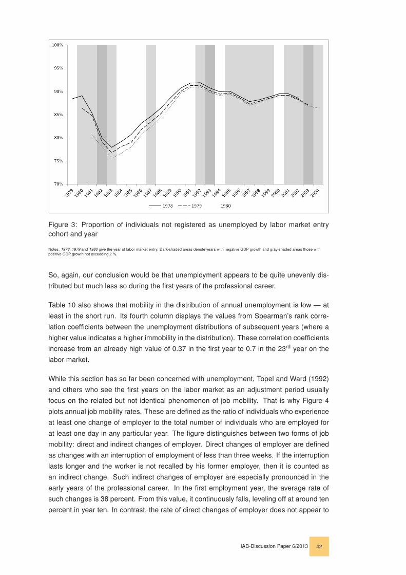
Figure 3: Proportion of individuals not registered as unemployed by labor market entrycohort and year

Notes: 1978, 1979 and 1980 give the year of labor market entry. Dark-shaded areas denote years with negative GDP growth and gray-shaded areas those withpositive GDP growth not exceeding 2 %.

So, again, our conclusion would be that unemployment appears to be quite unevenly dis-

tributed but much less so during the first years of the professional career.

Table 10 also shows that mobility in the distribution of annual unemployment is low — at

least in the short run. Its fourth column displays the values from Spearman’s rank corre-

lation coefficients between the unemployment distributions of subsequent years (where a

higher value indicates a higher immobility in the distribution). These correlation coefficients

increase from an already high value of 0.37 in the first year to 0.7 in the 23rd year on the

labor market.

While this section has so far been concerned with unemployment, Topel and Ward (1992)

and others who see the first years on the labor market as an adjustment period usually

focus on the related but not identical phenomenon of job mobility. That is why Figure 4

plots annual job mobility rates. These are defined as the ratio of individuals who experience

at least one change of employer to the total number of individuals who are employed for

at least one day in any particular year. The figure distinguishes between two forms of job

mobility: direct and indirect changes of employer. Direct changes of employer are defined

as changes with an interruption of employment of less than three weeks. If the interruption

lasts longer and the worker is not recalled by his former employer, then it is counted as

an indirect change. Such indirect changes of employer are especially pronounced in the

early years of the professional career. In the first employment year, the average rate of

such changes is 38 percent. From this value, it continuously falls, leveling off at around ten

percent in year ten. In contrast, the rate of direct changes of employer does not appear to


Table 10: Inequality and immobility in the distribution of annual unemployment

unemployment

Year on labor market Total sum (in million days) Inequality (Gini coefficients) Immobility (Spearman’s ρ)

1 8.1 0.9211 0.37312 11.7 0.9152 0.43853 18.5 0.8904 0.50024 24.0 0.8731 0.56055 26.2 0.8729 0.59476 24.7 0.8818 0.59807 22.2 0.8939 0.61018 20.1 0.9056 0.61549 17.8 0.9171 0.606210 14.8 0.9314 0.588211 12.2 0.9431 0.578912 10.8 0.9496 0.573913 11.4 0.9483 0.604714 13.2 0.9433 0.625815 14.7 0.9389 0.643616 15.9 0.9351 0.657417 17.2 0.9303 0.677318 18.5 0.9262 0.693219 18.5 0.9263 0.696420 17.3 0.9308 0.686421 16.4 0.9338 0.681522 16.7 0.9327 0.686823 18.5 0.9268 0.704924 20.7 0.9195 —

Notes: Year on labor market indicates the number of years since labor market entry. For every year, total sum (in million days) adds up the days of registeredunemployment over all individuals in the sample. Inequality reports Gini coefficients of total annual unemployment. These Gini coefficients include all zeros andare computed with the Stata command ineqdec0. Immobility gives Spearman’s ρ as a measure of the rank correlation between the distributions of total annualunemployment between consecutive years on the labor market.

be particularly high in the early years of the professional career.25

8.4 Local Average Treatment Effects and Average Causal Effects

In section 5 we implicitly assumed that causal effects are the same for everybody. Without

this assumption, two stage least squares estimates would have to be interpreted as local

average treatment effects, that is, as a treatment effect valid for those individuals who

experienced a higher level of early-career unemployment only because they suffered from

adverse initial labor market conditions (“compliers”). To assess who is really affected by

the instruments, we now go back to the first stage of the Tobit IV regression with both

instruments [column (6) of Table 4]. In Table 11 we re-run this regression separately for

subgroups defined by two of our covariates: initial occupation and industry. Coefficients

are ranked by size, and should be interpreted relative to the effects for the full sample of

29.43 for the local unemployment rate at graduation, and 42.93 for closure of the training

firm. Larger coefficients mean that the instruments’ effect on early-career unemployment

is stronger for the respective group than for the full sample, and vice versa.

For the district unemployment rate, Table 11 shows a clear pattern: graduates trained in

unskilled service, commercial, and manual occupations react more heavily to the instru-

ment than graduates in high-skilled occupations. Moreover, compliers are concentrated

in cyclical industries like construction, manufacturing, or energy and mining. In the case

of the second instrument, patterns are less clear for both the occupation and the sector

variables.

25 Unsurprisingly, direct changes of employer are more pronounced in years with favorable economic con-ditions, as indicated by the areas in Figure 4 that are not shaded gray or black. The opposite is true forindirect changes. Over the entire observation period, 13 percent of individuals continually stay with theirinitial employer. About 79 percent experience at least one direct change of employer.


Table 11: Different estimates of early-career unemployment — Characteristics of the com-pliant subpopulation

Instrument: unemployment rate plant closure

rank occupation

1 Skilled services -5.39 Skilled services 10.45(14.08) (38.66)

2 (Semi)professions 7.91 Skilled manual 31.65***(8.94) (5.39)

3 Agriculture 16.6 Unskilled services 32.51(16.01) (33.37)

4 Technicians and engineers 22.34*** Technicians and engineers 40.92**(7.99) (20.79)

5 Skilled commercial/Managers 27.97*** (Semi)professions 42.8(3.07) (44.16)

6 Skilled manual 29.00*** Agriculture 43.31(1.96) (27.43)

7 Unskilled services 32.71*** Skilled commercial/Managers 57.77***(12.48) (14.56)

8 Unskilled commercial 34.94*** Unskilled commercial 66.52**(8.62) (27.38)

9 Unskilled manual 35.64*** Unskilled manual 95.42***(7.44) (26.76)

rank sector

1 Non-profits/Households -28.55 Non-profits/Households -88.97(36.99) (64.50)

2 Financial intermediation 17.83** Energy/Mining -13.02(7.05) (102.13)

3 Agriculture 23.76 Financial intermediation 8.09(19.18) (29.77)

4 Other services 26.44*** Other services 18.25*(5.24) (10.74)

5 Transport and communications 27.53*** Trade 35.75***(10.61) (10.76)

6 Trade 28.79*** Agriculture 35.82(3.99) (71.24)

7 Public administration 30.50*** Construction 40.59***(10.96) (10.26)

8 Construction 30.85*** Manufacturing 49.63***(3.79) (7.97)

9 Manufacturing 31.06*** Transport and communications 108.60(2.28) (74.31)

10 Energy/Mining 35.01** Public administration 141.61***(17.00) (42.19)

Notes: Standard errors clustered at the establishment level in parentheses. * , (**), [***] indicates significance at the 10, (5), [1] % level. Displayed are first-stage estimates from Tobit IV regressions with a specification similar to the one in column (6) of Table 4 but conditional on subgroups by initial occupation orsector, respectively. In the full sample the coefficient on the district unemployment rate at graduation is 29.43 and 42.93 for the closure of the training firm. Allregressions are calculated with Smith and Blundell’s (1986) conditional maximum likelihood Tobit IV estimator. The delta method is used to compute standarderrors.


Figure 4: Job mobility rates

Notes: 1978, 1979 and 1980 give the year of labor market entry. Mobility rates are defined as the ratio of individuals who experience at least one change ofemployer to the total number of individuals who are employed for at least one day in any particular year. Direct changes of employer are defined as changes with aninterruption of employment of less than three weeks. If the interruption lasts longer and the worker is not recalled by his former employer, then it is counted as anindirect change. Dark-shaded areas denote years with negative GDP growth and gray-shaded areas those with positive GDP growth not exceeding 2 %.

Thus, plant closures appear to affect a broader range of the population than differences in

local labor market conditions. In this sense, the scarring effect derived with the help of the

district unemployment rate as instrument [column (9) of Table 2] is more “local”, while the

one estimated using plant closures [column (5) of Table 4] is closer to the average treatment

effect on the treated. Specifications using both instruments blend these effects into a single

statistic [column (6) of Table 4]. Since scarring effects are stronger for compliers relative

to the whole population, Tobit IV estimates might be interpreted as an upper bound for

the average treatment effect on the treated. Conversely, if all identifying assumptions hold,

Tobit estimates understate this treatment effect. Therefore, they could be seen as providing

a lower bound for the scarring effect of early-career unemployment.

Angrist and Imbens (1995) note that econometric applications of IV typically postulate a

hypothetical linear response function while the statistical literature on evaluation allows for

variable treatment intensity. They show that under the additional assumption of mono-

tonicity linear IV estimators can also be interpreted as an estimate of the average causal

effect of variable treatments. This effect is defined as a weighted average of the difference

between the outcomes of the treated, and what these outcomes would have been in the

absence of treatment.

To assess whether we can interpret our results along the lines of Angrist and Imbens

(1995), we first examine whether monotonicity holds. For this purpose, we compare the

cumulative distribution functions (CDFs) of early-career unemployment for groups defined


Figure 5: CDF of early-career unemployment by treatment status

Notes: The left panel depicts the early-career unemployment CDF for individuals whose initial unemployment rate was below or above average. The right-handpanel depicts the early-career unemployment CDF for individuals who were or were not separated from their training firm due to plant closure.

by treatment status. Angrist and Imbens (1995) show that if the CDFs cross neither for

the treatment nor for the control group, this suggests treatment is monotonous. Figure 5

plots the corresponding CDFs of early-career unemployment for our two instruments. For

illustrative purposes the first treatment is defined as a local unemployment rate above the

average unemployment rate over all labor market districts. The left panel of Figure 5 shows

that for any given value of early-career unemployment, the CDF for the group receiving this

treatment is above that for the control group. This is consistent with monotonicity. As is

evident from the right-hand panel of Figure 5, CDFs for the group of individuals separated

from their training firm because of plant closure, and the respective control group are closer

together. However, they do not cross either.

Under monotonicity, we can shed some light on how heterogeneous responses to treatment

are weighted to arrive at the average causal effects. This provides some additional insight

into which observations contribute to the eventual estimates. Angrist and Imbens (1995)

demonstrate that weights are proportional to the CDF differences between treatment and

control groups: for each level of early-career unemployment, mt1 = x, this difference is

the fraction of the population shifted by the instrument from having fewer than x days of

unemployment to experiencing at least x days. The average causal response weighting

function can be visualized by plotting levels of early-career unemployment against the dif-

ferences in the CDFs of early-career unemployment between treatment and control. This

is done in Figure 6 together with 99 percent confidence bands calculated pointwise with

the conventional formula for testing differences in proportions.


The left-hand panel of Figure 6 shows that the probability of not experiencing a single day

of early-career unemployment is about eight percentage points higher for individuals with

favorable local labor market conditions at graduation. Besides, above-average unemploy-

ment rates at graduation led around seven percent of the sample to experience early-career

unemployment of one year or longer. For 4.6 percent of individuals, they induced at least

two years of youth unemployment. The right-hand panel of Figure 6 repeats the compari-

son for the plant closure instrument. Here, the probability of experiencing no early-career

unemployment is about twelve percentage points higher for graduates who — at least po-

tentially — had the possibility to stay with their training firm. The panel also shows that the

proportion of individuals induced by plant closure to accumulate youth unemployment of

(at least) a given amount rapidly declines in the level of early-career unemployment.

A comparison of both panels of Figure 6 yields that IV estimates based on differences in

local labor market conditions seem to weigh observations more evenly than when plant

closure is the instrument. Thus, in line with findings by von Wachter and Bender (2006),

training firm closures might be seen as severe but relatively short-lived shocks. In con-

trast, differences in local labor market conditions affect the employment career less vehe-

mently but for a longer period. What both instruments have in common is that they induce

differences in early-career unemployment primarily at relatively short durations. This is

reassuring for our identification strategy because if longer unemployment durations had

been weighted more heavily, this could have been interpreted as the instruments picking

up effects of a permanently high propensity to experience unemployment, i.e. patterns of

serially correlated unobserved heterogeneity.

8.5 Censored Quantile Instrumental Variable Regression

Assume linearity in parameters and a conditional quantile function of the dependent vari-

able, m∗t2 =Qm∗t2(τ |mt1, w, ot1, ut2), (prime-age unemployment) at quantile τ that depends

on the regressor of interest, mt1, (early-career unemployment), a vector of exogenous co-

variates, w, (including a constant and possibly the censoring variable), a latent and unob-

served variable, ot1, which is correlated with both m∗t2 and mt1, and the error term, ut2,

with a conditional quantile of zero, Qut2(τ |mt1, w, ot1) = 0.26 Then, with τ ∈ [0, 1] indexing

the quantile and {i = 1, ..., N} indicating the individual, we arrive at the following system

of equations:

m∗i,t2 = mi,t1α(τ) + w′iβ(τ) + oi,t1γ(τ) + ui,t2, (5)

mi,t1 = w′iβ + zi,t0π + oi,t1, (6)

where α(τ), β(τ), and γ(τ) are parameters to be estimated. Further assume conditional

independence of ut2, and ot1, ut2 ∼ U(0, 1)|mt1, w, zt0, ot1, and ot1 ∼ U(0, 1)|w, zt0. As

long as we cannot control for ot1, estimates of α(τ) would be biased and inconsistent,

because ot1 would be absorbed by the new error term, “inducing endogeneity or selection

26 Chernozhukov and Hansen (2006) note that neither the hypothetical values ofm∗t2 which would evolve underrandom assignment of treatment nor its corresponding quantiles are actually observable if endogeneity ispresent. However, CQIV still allows us to recover the structural parameters of Qm∗

t2(τ |.).


Figure 6: Early-career unemployment CDF differences

Notes: The left panel depicts the early-career unemployment CDF difference by treatment status where treatment is defined as initial unemployment rates beingabove average. In the right panel, treatment is defined as plant closure of the training firm at graduation. Dotted lines are 99 % confidence intervals.

bias, so that the conditional quantile of selected [m∗t2] given the selected [mt1], is generally

not equal to the quantile of potential outcome” [Chernozhukov and Hansen (2006: p.494)].

While we cannot observe ot1 directly, we can estimate it from the residuals of Equation 6.

To accomplish this, we need to use the “instrumental variable” zt0, that is excluded from

Equation 5 but influences dt1 through π in Equation 6. This instrumental variable enables

us to control for any endogenous variation of dt1 in Equation 6, and thus to recover the

parameters of interest. This is why ot1 is known as the control term, and Equation 6 as the

control function.

Our study mainly uses labor market conditions at the time of graduation as instruments.

Therefore, ot1 could be interpreted as the marginal propensity to experience early-career

unemployment evaluated at the respective position in the distribution of prime-age unem-

ployment conditional on the quality of initial matching of apprentices to firms, and further

exogenous characteristics.

Additionally, we face a corner solution with positive probability mass at zero. That is why we

interpret m∗t2 as the latent amount of prime-age unemployment as opposed to the actually

observed amount of prime-age unemployment; i.e. Equation (4) holds.

The conditional quantile function of mt2 is

Qmt2(τ |X) = max(X ′ψ(τ), 0), (7)


where X ≡ [mt1, w, ot1], and ψ(τ) ≡ [α(τ), β(τ), γ(τ)]. Equation 7 holds because quan-

tiles are equivariant against monotone transformations, such as censoring. In the presence

of exogenous regressors, the model presented so far could be consistently estimated with

Powell’s (1986) estimator. Better applicability is achieved by the semi-parametric estima-

tor developed by Chernozhukov and Hong (2002), which is asymptotically as efficient as

Powell’s (1986) estimator but far less computationally demanding.

Chernozhukov, Fernández-Val and Kowalski (2011) combine Chernozhukov and Hong’s

(2002) estimator with a control function approach. The authors show that under mild reg-

ularity assumptions,√n-consistent and asymptotically normal estimates for ψ(τ) at every

quantile τ can be obtained by

ψ(τ) = arg minψ∈Rdim(X)

1

N

N∑i=1

I(S′iδ > k)ρτ (mi,t2 − X ′iψ). (8)

Here I(.) is an indicator function taking on unity when the expression holds, and zero

otherwise, ρτ (ut2) is Koenker and Bassett’s (1978) absolute asymmetric loss function,

X = x(mt1, w, ot1), S = s(X, 0), and both x(.) and s(.) are vectors of transformations

of (mt1, w, ot1), or (X, 0), respectively. I(S′δ > k) is called “selector” by Chernozhukov,

Fernández-Val and Kowalski (2011) because — by identifying uncensored observations

with censored predictions — it selects the subset of observations for which a linear form

of the conditional quantile function can be assumed. Unfortunately, linear programming

cannot be used to solve Equation 8. Instead, one may rely on an algorithm proposed by

Chernozhukov, Fernández-Val and Kowalski (2011) which augments the three-step proce-

dure of Chernozhukov and Hong (2002) by an additional step. The resulting four steps are

as follows:

Step 1. Run an OLS regression of mt1 on the instrument zt0 and exogenous regressors

w and obtain a prediction for the control term ot1 = Fd(,t1 |w, zt0) from the residuals. This

allows the construction of X = x(mt1, w, ot1).

Step 2. Identify the linear part of the conditional quantile function X ′ψ0(τ). To do so,

choose a subset of observations for which the conditional quantile line is “sufficiently”

above zero, {i : X ′iψ0(τ) > 0}. Estimating a logit model for the conditional probability

of non-censoring P (mt2 = 1|S),

P (mi,t2 = 1|Si) = Λ(S′iδ0), (9)

allows us to choose a sample, J0(c), that contains those observations which satisfy

J0(c) = {i : Λ(S′iδ0) > 1− τ + c}, (10)

with 0 < c < τ . Chernozhukov and Hong (2002) suggest choosing c, such that

#J0(c)/#J0(0) = 0.9.


Step 3. Run an ordinary quantile regression on subsample J0(c). This gives

ψ0(τ) = arg minψ∈Rdim(X)

∑i∈J0(c)

ρτ (mi,t2 − X ′iψ), (11)

a consistent but inefficient estimate. To gain efficiency, the subset of observations used in

Step 2 is updated by choosing J1(k) according to:

J1(k) = {i : X ′iψ0(τ) > k}, (12)

where the fitted values from Equation 11 are used, and the cut-off k plays a similar role to

c in Step 2.

Step 4. Finally, repeat Step 3 but this time on subsample J1(k).

8.6 Supplementary Tables and Figures

Figure 7: Quantile-quantile plot of early-career vs. prime-age unemployment, measured asproportion of potential time on the labor market


Table 12: Transition probabilities between certain positions in the distributions of early-career and prime-age unemployment

early-career unemployment

p51 p56 p61 p66 p71 p76 p81 p86 p91 p96 0prime-age to to to to to to to to to to tounemployment p55 p60 p65 p70 p75 p80 p85 p90 p95 1 p50

p61 to p65 5.8*** 6.4*** 6.2*** 6.2*** 6.4*** 6.4*** 6.4*** 5.8*** 5.0 3.2 42.2p66 to p70 5.2 6.0*** 6.2*** 6.6*** 6.8*** 6.8*** 7.0*** 6.8*** 6.2*** 4.4 38.0p71 to p75 5.0 5.4 6.0*** 6.8*** 6.8*** 6.6*** 7.0*** 8.6*** 6.4*** 5.2*** 36.2p76 to p80 5.0 5.4 5.6*** 6.2*** 6.4*** 6.8*** 7.4*** 7.8*** 7.0*** 5.8*** 36.6p81 to p85 4.6 4.8 5.8*** 6.6*** 6.8*** 7.4*** 8.2*** 8.8*** 8.2*** 8.2*** 30.6p86 to p90 4.2*** 4.6 5.6 5.8*** 6.2*** 7.4*** 8.0*** 9.6*** 9.4*** 10.4*** 28.8p91 to p95 3.4*** 3.8*** 4.8 5.4 6.0*** 7.2*** 8.6*** 11.0*** 11.8*** 15.8*** 22.2p96 to 1 2.2*** 2.6*** 3.2*** 4.0*** 4.8 5.8*** 7.2*** 10.0*** 13.4*** 32.2*** 14.60 to p60 64.6 61.0 56.6 52.4 49.8 45.6 40.2 31.6 32.6 14.8 37.1

Notes: All probabilities are given in percent. *** indicates significance at the 1 % level as indicated by Pearson’s chi-squared tests with the null hypothesis ofindependence between early-career and prime-age unemployment. The hypothesis that all rows and columns in the table are independent is rejected with anoverall χ2(361) = 2.7exp6 .

Table 13: Relation between early-career unemployment and later unemployment

employment yearsearly-career unemployment obs. later unemployment 9 to 12 13 to 16 17 to 20 21 to 24

0 to p50 413,569 occurrence 0.09 0.10 0.11 0.10mean amount 18.97 28.57 34.32 34.15

p51 to p60 82,962 occurrence 0.18 0.16 0.16 0.15mean amount 38.27 45.64 53.48 51.56





p96 to 1 41,273 occurrence 0.74 0.52 0.49 0.44mean amount 393.96 302.80 324.17 289.35

Notes: Occurrence is measured as the proportion of individuals registered as unemployed for at least one day within each time frame. Mean amount denotesthe mean total unemployment generated within each time frame.

Figure 8: Annual sample attrition rates (in %)

Notes: Annual rates of individuals that disappear from the observable part of the German labor market (in %) by year on the labor market.


Table 14: Estimates of prime-age unemployment — Different marginal effects from a TobitIV regression

(1) (2) (3) (4) (5)

Model Tobit IV

Marginal effect Average marginal Average marginal Marginal effects Average marginal Average marginal effectseffects on latent effects on observed on observed variable effects on positive on probability of

variable variable at the average observations being uncensored

Regression of prime-age unemploymentEarly-career unemployment 5.14*** 1.98*** 2.14*** 1.75*** 0.0010***

(0.60) (0.20) (0.25) (0.21) (0.0001)Age -22.87*** -8.79*** -9.53*** -7.77*** -0.0042***

(1.86) (0.70) (0.78) (0.64) (0.0004)Remuneration 2.06 0.79* 0.86 0.70 0.0004*

(1.28) (0.48) (0.53) (0.44) (0.0002)Size of training firm -4.41** -1.69** -1.83** -1.50** -0.0008**

(1.78) (0.71) (0.74) (0.60) (0.0004)Median wage of training firm -0.82 -0.32 -0.34 -0.28 -0.0002

(0.77) (0.30) (0.32) (0.26) (0.0001)Occupation (reference category: agricultural occupations)Unskilled manual occup. 42.56 16.37 17.74 14.47 0.0078

(36.74) (14.02) (15.31) (12.50) (0.0067)Skilled manual occup. 13.94 5.36 5.81 4.74 0.0026

(55.50) (21.27) (23.14) (18.87) (0.0102)Technicians and engineers 30.79 11.84 12.84 10.46 0.0057

(75.52) (28.87) (31.48) (25.69) (0.0138)Unskilled services -52.07 -20.03 -21.71 -17.70 -0.0096

(37.48) (14.38) (15.62) (12.74) (0.0069)Skilled services -32.36 -12.45 -13.49 -11.00 -0.0060

(54.37) (21.07) (22.67) (18.46) (0.0103)Semiprofessions 49.09 18.88 20.46 16.69 0.0091and professions (88.11) (33.61) (36.74) (29.99) (0.0160)Unskilled commercial oc-

cup.259.18*** 99.68*** 108.04*** 88.08*** 0.0480***

(72.96) (26.56) (30.37) (24.96) (0.0118)Skilled commercial occup. 129.27 49.72 53.89 43.94 0.0239and managers (89.09) (33.48) (37.13) (30.37) (0.0155)

Number of observations 739,432

Notes: Standard errors clustered at the district level in parentheses. * , (**), [***] indicates significance at the 10, (5), [1] % level. The Tobit IV regression is cal-culated with Smith and Blundell’s (1986) conditional maximum likelihood estimator. The instrument is the local unemployment rate at graduation. The followingare reported: in (1) the marginal effects on the latent amount of prime-age unemployment (i.e. the model’s coefficients); in (2) the average marginal effects onthe observed amount of prime-age unemployment; in (3) the marginal effects on the observed amount of prime-age unemployment if all explanatory variablestake on their average value; in (4) the average marginal effects on the observed amount of prime-age unemployment among the subpopulation for which prime-age unemployment is not at a boundary; in (5) the average marginal effects on the probability of being uncensored. Covariates are the same as in column (9) ofTable 2. For all factor variables the discrete first differences from the base categories are calculated.

Table 15: Different estimates of prime-age unemployment — Tobit robustness regressions

(1) (2) (3) (4) (5) (6)

Spe

cific

atio

n

Une

mpl

oym

enti

nor

igin

attr

ansi

tion

asco

ntro

l

Min

imum

unem

ploy

men

tin

early

care

eras

cont

rol

Atl

east

one

obse

rvat

ion

durin

gla

stfo

urye

ars

Less

than

six

year

sof

seas

onal

empl

oym

ent

Non

empl

oym

entI

inst

ead

ofun

empl

oym

ent

Non

empl

oym

entI

Iin

stea

dof

unem

ploy

men

t

Model Tobit Tobit Tobit Tobit Tobit Tobit

Regressions of prime-age unemployment [prime-age nonemployment in (5) and (6)]Early-career unemployment 0.57*** 0.57*** 0.61*** 0.50*** — —

(0.01) (0.01) (0.01) (0.01)Early-career nonemployment — — — — 0.58*** 0.30***

(0.01) (0.01)

Other variables included in regressionsDistrict dummies Yes Yes Yes Yes Yes YesUnemp. at transition (current) No Yes Yes Yes Yes YesUnemp. at transition (origin) Yes No No No No NoMinimum unemp. in early career No Yes No No No No

Number of observations 740,394 739,432 648,644 652,206 739,432 739,432

Notes: Standard errors clustered at the district level in parentheses. *** indicates significance at the 1 % level. All regressions are performed with Hansen,Heaton and Yaron’s (1996) continuously updated GMM estimator implemented in the Stata command ivreg2 by Baum, Schaffer and Stillman (2003, 2007), andreport the average marginal effects on the observed amount of prime-age unemployment [prime-age nonemployment in (5) and (6)]. The delta method is usedto compute standard errors. Unless otherwise noted, covariates are the same as in column (5) of Table 2. In (1) the local unemployment at the transition fromyouth to prime age for the district of the last apprenticeship spell is used as a control variable; in (2) the minimum local unemployment rate during the early ca-reer is used as a control variable; in (3) individuals who are not observed during the last four years of their prime age are excluded; in (4) individuals with morethan five years of seasonal employment are excluded; in (5) and (6) early-career and prime-age nonemployment modeled on the definitions by Fitzenberger andWilke (2010), and Schmieder, von Wachter and Bender (2012), respectively, are used instead of early-career and prime-age unemployment.


Table 16: Number of years with seasonal employment spells

number of years with seasonal employment spells observations of sample in % share

0 430,655 47.742 211,571 23.453 50,697 5.624 74,522 8.265 36,829 4.086 30,043 3.337 19,544 2.178 13,928 1.549 9790 1.0910 or more 24,551 2.72

total 902,130 100

Notes: Seasonal employment denotes two or more employment spells that last for at least two but less then eleven months, and end at about the same time inconsecutive calendar years; cf. Del Bono and Weber (2008).


-0.012

-0.010

-0.008

-0.006

-0.004

-0.002

0.000

0

2

4

6

8

10

12

14

16

18

20

50 55 60 65 70 75 80 85 90 95

Co

eff

icie

nt

Percentile

Coefficients of early-career unemployment

Early-career unemployment (left axis)

Early-career unemployment squared (right axis)

1000

2000

3000

4000

5000

6000

7000

ag

e u

ne

mp

loy

me

nt

(da

ys)

Marginal effects of early-career unemployment

0

1000

2000

100 200 300 400 500 600 700 800 900 1000

Pri

me

-ag

e u

ne

mp

loy

me

nt

(da

ys)

Early-career unemployment (days)

50th percentile 60th percentile 70th percentile

80th percentile 90th percentile

Figure 9: Different estimates of prime-age unemployment — Quadratic censored quantileinstrumental variable regressions

Notes: The top panel depicts coefficients of early-career unemployment, and early-career unemployment squared from quadratic censored quantile instrumentalvariable regressions that use Chernozhukov, Fernández-Val and Kowalski’s (2011) four-step procedure. The bottom panel displays the respective marginal effects onthe observed amount of prime-age unemployment across quantiles of prime-age unemployment and levels of early-career unemployment. All quantile regressionsare calculated using Stata’s qreg command. The instrument is the local unemployment rate at graduation. Covariates are the same as in column (9) of Table 2.



Recently published

No. Author(s) Title Date 20/2012 Dauth, W.

Südekum, J. Profiles of local growth and industrial change: Facts and an explanation

9/12

21/2012 Antoni, M. Heineck, G.

Do literacy and numeracy pay off? On the rela-tionship between basic skills and earnings

9/12

22/2012 Blien, U. Messmann, S. Trappmann, M.

Do reservation wages react to regional unem-ployment?

9/12

23/2012 Kubis, A. Schneider, L.

Human capital mobility and convergence: A spa-tial dynamic panel model of the German regions

9/12

24/2012 Schmerer, H.-J. Skill-biased labor market reforms and interna-tional competitiveness

10/12

25/2012 Schanne, N. The formation of experts’ expectations on labour markets: Do they run with the pack?

10/12

26/2012 Heining, J. Card, D. Kline, P.

Workplace heterogeneity and the rise of West German wage inequality published in: The Quarterly Journal of Economics, (2013)

11/12

27/2012 Stops, M. Job matching across occupational labour markets

11/12

28/2012 Klinger, S. Weber, W.

Decomposing Beveridge curve dynamics by correlated unobserved components

12/12

29/2012 Osiander, Ch. Determinanten der Weiterbildungsbereitschaft gering qualifizierter Arbeitsloser

12/12

1/2013 Fuchs, J. Weber, E.

A new look at the discouragement and the added worker hypotheses: Applying a trend-cycle de-composition to unemployment

1/13

2/2013 Nordmeier, D. Weber, E.

Patterns of unemployment dynamics in Germany 4/13

3/2013 Zabel, C. Effects of participating in skill training and work-fare on employment entries for lone mothers receiving means-tested benefits in Germany

4/13

4/2013 Stephani, J. Does it matter where you work? Employer characteristics and the wage growth of low-wage workers and higher-wage workers

5/13

5/2013 Moczall, A. Subsidies for substitutes? New evidence on deadweight loss and substitution effects of a wage subsidy for hard-to-place job-seekers

5/13

As per: 22.05.2013 For a full list, consult the IAB website

http://www.iab.de/de/publikationen/discussionpaper.aspx

http://www.iab.de/183/section.aspx/Publikation/k120913j01

http://www.iab.de/183/section.aspx/Publikation/k120918301












http://www.iab.de/183/section.aspx/Publikation/k130328n06




http://www.iab.de/de/publikationen/discussionpaper.aspx

Imprint

IAB-Discussion Paper 6/2013

Editorial addressInstitute for Employment Research of the Federal Employment AgencyRegensburger Str. 104D-90478 Nuremberg

Editorial staffRegina Stoll, Jutta Palm-Nowak

Technical completionJutta Sebald

All rights reservedReproduction and distribution in any form, also in parts, requires the permission of IAB Nuremberg

Websitehttp://www.iab.de

Download of this Discussion Paperhttp://doku.iab.de/discussionpapers/2013/dp0613.pdf

ISSN 2195-2663 For further inquiries contact the author:

Matthias UmkehrerPhone +49.911.179 6211E-mail [email protected]

http://www.iab.de

http://doku.iab.de/discussionpapers/2013/dp0613.pdf

mailto:matthias.umkehrer%40iab.de?subject=

The scars of youth - IAB

Documents